finite element crack width computations with a thermo
TRANSCRIPT
1
Finite element crack width computations with a thermo‐hygro‐mechanical‐hydration model for concrete
A Jefferson*, R Tenchev†, A Chitez*, I Mihai*, G Coles
†, P Lyons
†, J Ou**
* Cardiff University, The Parade, Cardiff, UK, CF24 3AA, [email protected], www.cardiff.ac.uk † LUSAS, Forge House, High Street, Kingston‐upon‐Thames, Surrey, UK, [email protected], www.lusas.com ** Formerly Cardiff University
Key words: Concrete, plasticity, damage, hydration, shrinkage, creep, cracking.
Abstract: The paper presents an overview of a finite element approach for the analysis of the thermo‐hygro‐mechanical‐hydration behaviour of concrete structures. The thermo‐hygro component considers the mass balance equation of moisture as well as the enthalpy balance equation, and uses two primary variables, namely the capillary pressure and temperature. Heat of hydration is simulated using the approach of Schlinder and Folliard. The basic mechanical model simulates directional cracking, rough crack closure and crushing using a plastic‐damage‐contact approach. Hydration dependency is introduced into the mechanical constitutive model. The material data from the Concrack benchmark (CEOS.fr,2013) are considered with the model. This includes data on adiabatic temperature changes during curing, changing elastic properties during curing, shrinkage and creep. The model, as implemented in the finite element program LUSAS, is used to analyse the Concrack benchmark beam RL1. Particular attention is paid to crack openings and the difference between predicted crack openings from analyses with and without time dependent effects. It is concluded that ignoring time dependent effects can result in a significant under‐estimate of crack openings in the working load range.
1 INTRODUCTION
Designers and analysts need to be able to predict the size and disposition of cracks in reinforced concrete elements, since satisfaction of code crack width limits is an important design criterion. There has been relatively little focus on accurate crack width prediction in the vast amount of work undertaken in the finite element modelling of reinforced concrete structures over the past 40 years. One option for obtaining crack widths is to use a model in which crack openings are computed explicitly. Such models include approaches with embedded cohesive elements (Tijssens et al. 2000), approaches which model strong discontinuities in meshes (Oliver et al. 2003) and element free methods (Rabczuk & Belytschko 2007). Whilst effective, these methods are not generally available in commercial codes and continue to present challenges when complex 3D structures are considered. Non‐local approaches have been adopted to regularise constitutive models with respect to mesh grading. Dufour et al. (2008) proposed a method for extracting crack widths from a non‐local strain field, in which a non‐local effective strain variable is equated to a regularised effective strain derived from an assumed discontinuity. Other authors have used detailed finite element models to aid the understanding of cracking behaviour in laboratory scale experiments (Wu & Gilbert 2009; Tammo et I. 2009). Sellier et al. (2013) presented an approach for extracting crack openings from continuum elements when using a plastic‐damage model for concrete. In this work they demonstrated that reasonable crack openings can be extracted for a range of unreinforced and reinforced concrete examples using their approach.
2
Crack openings are dependent not only upon mechanical loading and the hardened properties of concrete but also on the curing history and the material’s time dependent behaviour. In order to simulate such behaviour with finite elements, models need to account for hydration, shrinkage and creep (Gawin et al. 2006). In addition, the mechanical constitutive behaviour varies during the curing period, with the elastic properties, strength parameters and non‐linear stress‐strain behaviour all being dependent on the degree of hydration. This paper describes a thermo‐hygro‐mechanical‐hydration (THMH) model for concrete. The overall model comprises a set of sub‐models, which are combined for simulating plain and reinforced concrete structures. There are several unique aspects to the work described here but much existing work has been used as a basis for the various sub‐models. The approach to simulating hygro‐thermal behaviour owes much to the work of Gawin et al. (2006), with the exception that only one fluid phase is considered rather than two. This is possible due to the assumption that the gas pressure is maintained at atmospheric. The hydration model of Schindler & Folliard (2005) is used and the hydration dependent expressions for elastic constants and uniaxial strengths are based on those given by de Schutter (2002). The creep model builds on the ideas Bazant et al.’s (1997) solidification model but introduces the idea of two material states and extends the ideas of solidification to long term aging. The basic mechanical model is a new smoothed plastic‐damage‐contact model (Jefferson & Mihai 2013) which is here further developed with the introduction of hydration dependent plasticity and damage evolution functions. The mechanics model employs a local directional fracture strain which, along with a directionally dependent element characteristic length, is used to compute crack openings.
The paper considers the analysis of one of the Concrack benchmark problems (designated RL1) from the French CEOS.fr project (CEOS.fr 2013) using the new THMH model implemented in the finite element program LUSAS. The primary purpose of the paper is to present an analysis of the RL1 beam with and without time‐dependent behaviour and to address the question of how much these time‐dependent effects affect the crack openings and the overall response predicted by the non‐linear finite element model.
The components of the model are presented in outline in Sections 2‐5 and these are followed by a presentation of the analysis and associated discussion in Section 6.
2. GOVERNING HYGRO‐THERMAL (HT) EQUATIONS
An essential element of the model is the hygro‐thermal component. This employs the following mass balance equations for liquid water and water vapour:
w w v hm m J (1)
v vv m J (2)
where is the rate of mass transfer during evaporation of liquid water, is the rate of change of liquid
water mass due to hydration, is the averaged density of the phase ( = w or v), n is the
capillary porosity of the medium, is the degree of saturation of phase , is the bulk density of phase.
The superior dot denotes the time derivative with respect to the solid skeleton and J denotes the mass
flux of phase . The macroscopic enthalpy balance equation for the multi‐phase medium is as follows:
T v v hCT m H Q J (3)
3
where, Jw is the heat flux, T is the temperature of the medium, ∑ is the thermal capacity, Hv
is the specific enthalpy of evaporation and is the rate of heat generation of hydration. In the current model there is no constitutive equation for , since this term is eliminated by combining equations (1) and (2) into a single moisture mass‐balance equation. Two separate mass‐balance equations are required if both dry air and water vapour are considered. However, Bary et al. (2008) proposed a formulation in which the gas phase is not considered explicitly. The present authors also use a single moisture mass balance equation and achieve this by considering that the gas pressure is constant at atmospheric pressure. This results in a formulation in which capillary pressure (Pc) and temperature (T) are the primary variables. The moisture and thermal flux boundary conditions are provided by the equations (4) and (5) respectively.
0w v wv c v venvq J J n (4)
0T v w T c envH q T T J J n (5)
where n is normal vector to the boundary flux, qwv and qT are the water phase and heat boundary fluxes, c
and c are temperature and moisture boundary transfer coefficients, and venv and Tenv are the environmental water vapour density and temperature respectively. The HT model requires a set of standard constitutive equations (Gawin et al. 2006, Lewis and Schrefler 1998) that are included here in Appendix A.
3. HYDRATION MODEL
The curing of the cementitious material is described by Schindler & Folliard’s (2005) hydration model and is expressed in terms of the degree of hydration :
∞ (6)
in which the ultimate degree of hydration is given by 1.031 /0.5 0.3 1.0
0.194 /
FA slag
w cp p
w c; w/c is
the water cement ratio; sf and sf are parameters which depend on the cement type and te is the effective
time given by 0
1 1( ) exp
tE
e rr
At T t
R T T, Tr and T are reference (294K) and current temperatures
in Kelvin respectively, AE is the activation energy and R is the universal gas constant. The heat generation rate is given by
1 1( ) ( ) exp
sf
h u c sf ee r
EQ t H C t
t R T T (7)
The present model also makes use of the relative degree of hydration, defined as r= / (8)
de Schutter (2002) introduced a percolation threshold (0 ) into the expression for the relative degree of
4
hydration, such that r takes a value of zero for values of 0. This, when combined with the expressions in the following section, simulates the fact that concrete has negligible stiffness until a solid skeleton has percolated through the body of the concrete. In this work, an alternative approach is used in which all
strains are treated as viscous until concrete reaches a higher threshold (denoted c), after which the
material stiffness is based directly on the volume of solidified material, as explained below. c is generally taken to be 0.35.
4 HYDRATION DEPENDENT MECHANICAL BEHAVIOUR
4.1 Hydration dependent properties
The expressions adopted for the variation of basic mechanical properties with the degree of hydration are based on those given by de Schutter (2002) and de Schutter and Taerwe (1997), although, as explained
above, a different definition of r is used here. These are as follows
( ) Ecr f rE E
(9)
( ) fc
f
c
c r c rf f
(10)
( ) ft
f
c
t r t rf f
(11)
( ) Gf
f
cf r f rG G (12)
in which E is Young’s modulus, fc is the uniaxial compressive strength, ft is the tensile strength, subscript f denotes the fully cured value and the constants take the following values CE=0.7, Cfc=1.5, Cft=1 and CGf=1.5.
Equation (9) may be alternatively written
( )r r fE v E
(13)
in which v is the volume of hardened material and thus
Ecr rv (14)
4.2 Plastic‐damage‐contact model
The mechanical constitutive model uses the ideas from the plastic‐damage‐contact model of Jefferson (2003) but the model has recently been modified to make it more robust. The basic stress‐strain relationship for the model is given by
p
j
nT
e p tm jj 1
( )
σ D ε ε ε N ε
(15)
where is the stress tensor (in vector form), is the strain vector, jε
denotes the fracture strains for crack
j and np is the number of crack planes at an element integration point, Nj is the stress transformation
matrix, p is a plastic strain vector and tm denotes all time dependent strains (i.e. from shrinkage, creep and thermal effects). The local strains are derived from a local crack‐plane constitutive model in which the local stress (σ )
comprises a damaged (d) and an undamaged (u) component as follows;
u d1 σ σ σ (16)
5
in which ([0,1]) is a damage parameter.
The damage parameter is a function of an effective local strain parameter , which in turn is a function of
the local strains (ε ) (Jefferson, 2003). The crack band approach of Bazant and Oh (1983) is adopted to
regularise the model with respect to mesh grading.
This local stresses are related to the local strains (ε ) by the following relationship, in which crack number
subscripts have been omitted for clarity
o1 H( ) ( ( )) σ Dε ε Dε ε (17)
where is a contact surface function in relative strain space, H is a contact potential reduction function,
both of which are given in Jefferson (2003); oε is a local offset strain function (Jefferson et al. 2014) andD
is the local elasticity matrix, which in 2D takes the form E 0
0 G
D , where E and G are Young’s modulus
and the shear modulus of the uncracked concrete respectively.
The local fracture strain, i.e. the inelastic component of local strain, may be derived from (17) to be
1o s oH( ) ( ( ))
1 1
ε D σ ε ε ε C σ ε (18)
Using (18) in (15) and noting that the local stress vector is the transformed Cartesian stress vector (i.e.
σ Nσ ), the overall stress may be given by
p p
j j
-1n nT T
e j s j e p j oj 1 j 1
σ I D N C N D ε ε N ε
(19)
The basic constitutive model is described in Jefferson (2003), which gives details of the damage evolution, local damage surface and contact functions. Details of the revised contact component is described in Jefferson et al (2014) with further details being given in a forthcoming journal publication by the authors.
The plasticity functions in the constitutive model are unchanged from those of Jefferson (2003). However, hydration dependency has now been added to allow for the change in plastic behaviour during curing. This is applied to the friction hardening parameter that governs the slope of the yield surface and plastic potential in octahedral stress space (see Appendix B).
The plasticity sub‐model included friction hardening based on the following evolution function.
1 20
01
( ) 1c c
p pc c
c
ZZ Z e e
a
(20)
in which is a work hardening parameter which has a maximum value p.
Hydration dependency is achieved by making cc2 a function of r, as follows;
6
2 22 2(1 ) c a c a rc c fc c c c (21)
where 21 2
2
2 1 and 1
1
cc c
c
cc cc
c cc
c ec a e e
e.
The uniaxial strain at peak compressive stress (c) is given by
1 11r c c rc cfc c (22)
cc1 is taken initially as 1/3 and cf is the value of c for fully cured concrete (typically = 0.0022).
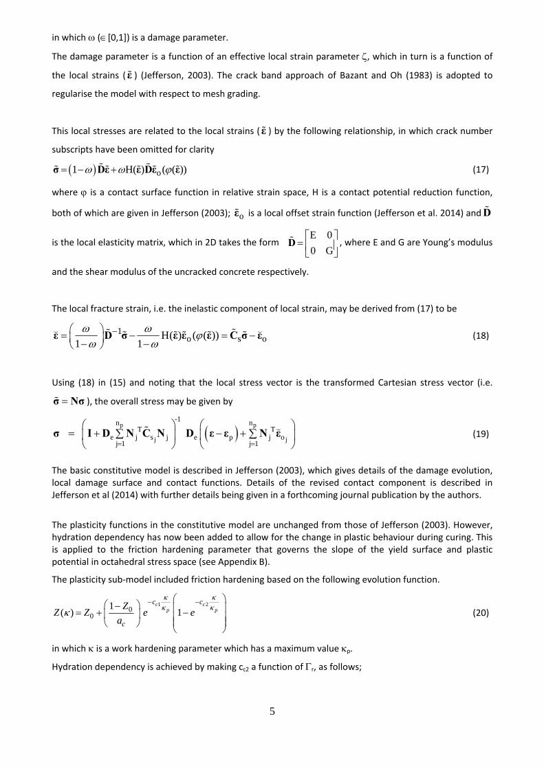
Yi et al. (2002) studied the effect of age on the stress‐strain properties of concrete. A comparison between predictions using the new plasticity model component and a set of Yi et al.’s experimental data is shown in Figure 1.
Figure 1. Experimental and numerical response with varying degrees of hydration
5. CREEP AND SHRINKAGE
The following section describes the essential features of the creep and shrinkage models. A much fuller description is provided in a forthcoming publication by the authors, in which an approach for simulating Pickett’s effect (or drying creep) is also described. 5.1 Creep model
The creep model is based on three main assumptions:
(i) concrete exhibits both short term and long term creep behaviour; over time, the gradual packing of the CSH blocks (Jennings 2008) increases the proportion of the material associated with the latter;
(ii) material always hardens in a stress free (or fluid pressure) state, as per Bazant et al.’s (1997) solidification theory; and
0.0
5.0
10.0
15.0
20.0
25.0
0.0000 0.0010 0.0020 0.0030 0.0040 0.0050 0.0060
Stress (MPa)
Strain
15.3 Hrs. Exp
2 Days. Exp
28 Days. Exp
15.3Hrs Numer
2 Days Numer
28 Days Numer
7
(iii) material elemental volumes mature from the short term to the long term state without changing stress.
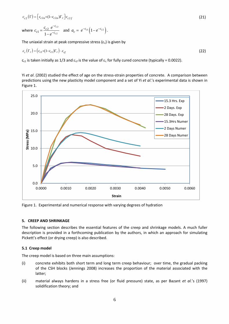
A further assumption in solidification theory is that a component of hardened material forms with the elastic properties of the fully cured concrete. The rheological model associated with this creep model is represented in Figure 2.
Figure 2. Creep rheological model The basic stress‐strain relationship for the creep model is as follows
f m e vsT1 v v σ I D ε ε (23)
j j j
3
vsT S vS sS L vL sLj 1
1
ε ε ε ε ε (24)
in which f = wet concrete fluid pressure (always assumed to be 0 in the present work), Im is the vector
denoting hydrostatic components, v=r0.7 is the proportion of solidified material, =proportion of long term
material component, S=elastic proportion of short‐term component, Li=are the relative proportions of
the long‐term material components, vε are the viscous strains , sε are the solidification‐aging strains and
subscript represents S (short‐term) or L (long‐term). It is noted that [0,1], j
3
Lj 1
1
and that 3vL ε 0 ,
since the third component of the long term component is elastic.
The proportion factors are set to the following fixed values
TS L0.85, 0.2 0.2 0.6 β (25)
These values of were determined in a parametric identification exercise, in which the viscous strains from equation (24) where matched with the creep strains from Eurocode 2 (EC2,2008), for a range of concretes and loading ages.
The solidification strains Sε account for the fact that each component of new material forms at the fluid
pressure and that when an elemental volume of material matures from the short term to the long‐term component the stress in that elemental volume doesn’t change.
S (1‐)Ef (1‐S )(1‐)Ef
(1‐S )(1‐)S
Short term material (S)
(1‐v)
L3 Ef
L1 Ef
L1 EfL1
L2 Ef
L1 EfL 2
v
(1‐)
Long term material (L) Fluid
8
The viscosities are related to the relaxation time parameters as follows;
fE
(26)
The model has been designed to use basic creep factors from other well established models and in this work the basic creep model from Eurocode 2 is used (EC2 2008).
At any time (t), the creep factor () and are computed from the following equations
2828 age w
r
v(t) S
v( )
(27)
3
SL S
1 11
1 1
(28)
where 28 is the ultimate basic creep factor from Eurocode 2 for a specimen loaded at 28 days,
age(t) is based on the EC2 aging factor, but normalised to the 28 day value. Furthermore, it is only applied
for t28 days. v28 is the volume of solidified material at 28 days. In the present implementation is limited
to the range 0.10.99 There is considerable experimental evidence to suggest that creep behaviour in tension is different from that in compression. Neville et al. (1983) discussed 16 sets of experiments which explored the differences between tensile and compressive creep and showed that in some situations compressive creep was greater than tensile creep, whilst in others the opposite was found to be the case. There have been a number of more recent investigations to further explore tensile creep behaviour; which includes work by Kolver (1999), Østergaard et al (2001), Rossi et al. (2012) and Ranaivomanana et al. (2013). Most recently, Hilaire (2013) have proposed a creep model which includes a single parameter to allow for the difference between tensile and compressive creep. No attempt has been made in the present model to account for the difference between tensile and compressive creep, nor to allow for temperature dependent creep (Benboudjema F, Torrenti, 2008); it is however acknowledged that in some situations these factors can be very significant. The viscous update of each Maxwell arm is undertaken using the algorithm given by Simo & Hughes (1998). 5.2 Shrinkage model Autogenous and drying shrinkage are computed from changes in the degree of saturation and degree of hydration. It has been found experimentally that, once hydration is complete, there is a remarkably linear relationship between weight loss and drying shrinkage for a normal environmental range of humidity (Barr
et al. 2003). Therefore, within this range, the drying shrinkage rate ( ds ) is based on the rate of change of
moisture content ( wS ). When the concrete is not fully cured, the aggregate restrains the shrinkage of the
hardened cement paste relatively more than in the fully cured case. Furthermore, at early ages, the volumetric tensile stresses that develop in the cement paste, due to the restraint from the aggregate phase, will tend to reduce rapidly due to the effects of early age creep. Thus what is measured as early age shrinkage in concrete is in fact a combination of creep, shrinkage and restraint effects within the phases of the composite material. To allow for this, a ‘degree of hydration’ term has been added to the shrinkage rate equation. Also adding a term for chemical shrinkage gives the following expression for the total shrinkage rate
sh ds w cs r rS (29)
9
in which ds and cs are constants controlling the amount of drying and chemical shrinkage respectively.
The authors’ justification for including r in equation (29) is not only the aforementioned mechanisms but also because it was found that this improved predictions of autogenous shrinkage. However, it is noted that in other work different trends for shrinkage rates during hydration have been reported (Xi and Jennings, 1997).
6 CONCRACK BENCHMARK
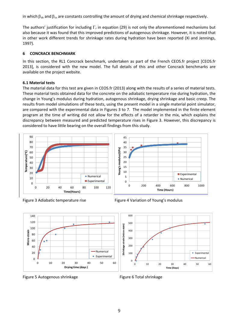
In this section, the RL1 Concrack benchmark, undertaken as part of the French CEOS.fr project [CEOS.fr 2013], is considered with the new model. The full details of this and other Concrack benchmarks are available on the project website. 6.1 Material tests The material data for this test are given in CEOS.fr (2013) along with the results of a series of material tests. These material tests obtained data for the concrete on the adiabatic temperature rise during hydration, the change in Young’s modulus during hydration, autogenous shrinkage, drying shrinkage and basic creep. The results from model simulations of these tests, using the present model in a single material point simulator, are compared with the experimental data in Figures 3 to 7. The model implemented in the finite element program at the time of writing did not allow for the effects of a retarder in the mix, which explains the discrepancy between measured and predicted temperature rises in Figure 3. However, this discrepancy is considered to have little bearing on the overall findings from this study.
Figure 3 Adiabatic temperature rise Figure 4 Variation of Young’s modulus
Figure 5 Autogenous shrinkage Figure 6 Total shrinkage
0
10
20
30
40
50
60
70
80
90
0 20 40 60 80 100 120
Temperature(oC)
Time(Hours)
Numerical
Experimental 0
5
10
15
20
25
30
35
40
45
0 200 400 600 800 1000
Young's modulus(GPa)
Time (Hours)
Experimental
Numerical
0
20
40
60
80
100
120
140
0 10 20 30 40 50 60
Micro‐strain
Drying time (days )
Numerical
Experimental
0
100
200
300
400
500
600
0 10 20 30 40 50 60
Shrinkage
strain (m
icro‐stain)
Time (Days)
Experimental
Numerical
10
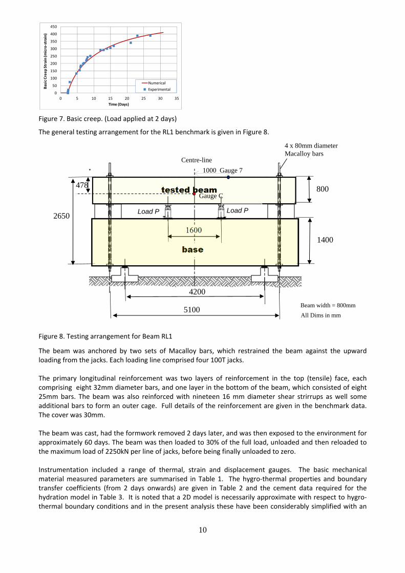
Figure 7. Basic creep. (Load applied at 2 days)
The general testing arrangement for the RL1 benchmark is given in Figure 8.
Figure 8. Testing arrangement for Beam RL1
The beam was anchored by two sets of Macalloy bars, which restrained the beam against the upward loading from the jacks. Each loading line comprised four 100T jacks. The primary longitudinal reinforcement was two layers of reinforcement in the top (tensile) face, each comprising eight 32mm diameter bars, and one layer in the bottom of the beam, which consisted of eight 25mm bars. The beam was also reinforced with nineteen 16 mm diameter shear strirrups as well some additional bars to form an outer cage. Full details of the reinforcement are given in the benchmark data. The cover was 30mm.
The beam was cast, had the formwork removed 2 days later, and was then exposed to the environment for approximately 60 days. The beam was then loaded to 30% of the full load, unloaded and then reloaded to the maximum load of 2250kN per line of jacks, before being finally unloaded to zero. Instrumentation included a range of thermal, strain and displacement gauges. The basic mechanical material measured parameters are summarised in Table 1. The hygro‐thermal properties and boundary transfer coefficients (from 2 days onwards) are given in Table 2 and the cement data required for the hydration model in Table 3. It is noted that a 2D model is necessarily approximate with respect to hygro‐thermal boundary conditions and in the present analysis these have been considerably simplified with an
0
50
100
150
200
250
300
350
400
450
0 5 10 15 20 25 30 35
Basic Creep Strain (m
icro‐strain)
Time (Days)
Numerical
Experimental
1600
4200
5100
1400
800
4 x 80mm diameter Macalloy bars
2650
tested beam
base
All Dims in mm
Beam width = 800mm
Load PLoad P
Centre-line
1000 Gauge 7
Gauge C
478
11
(effectively) impermeable and isolated lower boundary being applied during the first 2 days after casting.
Table 1. Concrack RL1 material data
Concrete properties Reinforcement properties
Ec GPa
fc MPa
ft MPa
Gf N/m
uls ds Strain
cs Strain
T
x10‐6
Es GPa
fy MPa
40.2 0.19 63.7 4.65 150 0.694 900 100 10 200 0.19 500
Table 2. Thermo‐hygro properties of concrete and boundary transfer coefficients
k
2/ /W m K m
C J/(kgK)
Kg/m3
K m2
n0 n c
W/(m2K) c
(m/s)
1.7 900 2410 1.7x10‐20 0.19 0.11 15 0.8 where k=thermal conductivity, C=specific heat capacity, =density, K=Intrinsic permeability and n0 & n are the initial and final porosities respectively.
Table 3. Cement data for Schlinder and Folliard hydration model
C3S (%) C2S (%) C3A (%) C4AF (%) SO3 (%) MgO (%) 2/ (%)CaO SiO Blaine index m2/kg
69.18 9.45 8.45 6.97 3.27 2.1% 3.06 415.4 in which standard notation is used for cement compounds (Schlinder and Folliard, 2005)
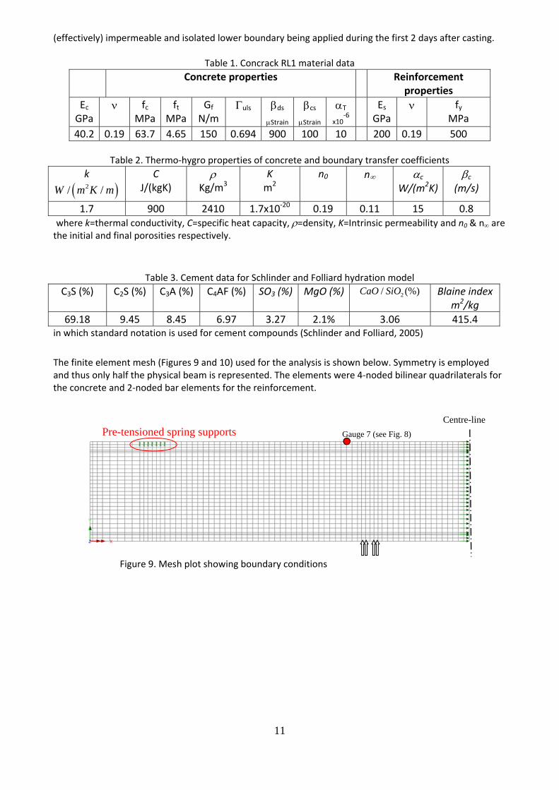
The finite element mesh (Figures 9 and 10) used for the analysis is shown below. Symmetry is employed and thus only half the physical beam is represented. The elements were 4‐noded bilinear quadrilaterals for the concrete and 2‐noded bar elements for the reinforcement.
Figure 9. Mesh plot showing boundary conditions
Centre-line Pre-tensioned spring supports Gauge 7 (see Fig. 8)
12
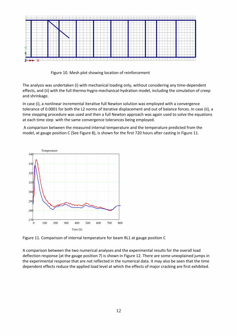
Figure 10. Mesh plot showing location of reinforcement
The analysis was undertaken (i) with mechanical loading only, without considering any time‐dependent effects, and (ii) with the full thermo‐hygro‐mechanical‐hydration model, including the simulation of creep and shrinkage.
In case (i), a nonlinear incremental iterative full Newton solution was employed with a convergence tolerance of 0.0001 for both the L2 norms of iterative displacement and out of balance forces. In case (ii), a time stepping procedure was used and then a full Newton approach was again used to solve the equations at each time step with the same convergence tolerances being employed.
A comparison between the measured internal temperature and the temperature predicted from the model, at gauge position C (See Figure 8), is shown for the first 720 hours after casting in Figure 11.
Figure 11. Comparison of internal temperature for beam RL1 at gauge position C
A comparison between the two numerical analyses and the experimental results for the overall load deflection response (at the gauge position 7) is shown in Figure 12. There are some unexplained jumps in the experimental response that are not reflected in the numerical data. It may also be seen that the time dependent effects reduce the applied load level at which the effects of major cracking are first exhibited.
0 100 200 300 400 500 600 700 800270
280
290
300
310
320
330
340Temperature
Time [h]
13
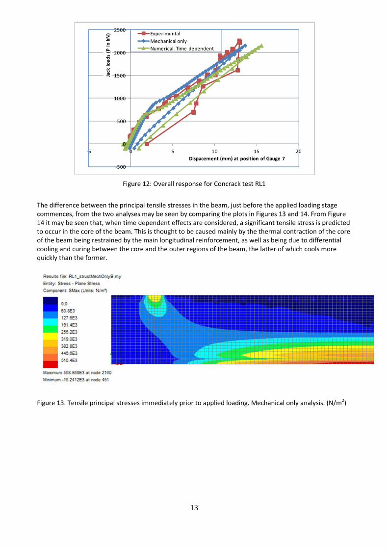
Figure 12: Overall response for Concrack test RL1
The difference between the principal tensile stresses in the beam, just before the applied loading stage commences, from the two analyses may be seen by comparing the plots in Figures 13 and 14. From Figure 14 it may be seen that, when time dependent effects are considered, a significant tensile stress is predicted to occur in the core of the beam. This is thought to be caused mainly by the thermal contraction of the core of the beam being restrained by the main longitudinal reinforcement, as well as being due to differential cooling and curing between the core and the outer regions of the beam, the latter of which cools more quickly than the former.
Figure 13. Tensile principal stresses immediately prior to applied loading. Mechanical only analysis. (N/m2)
‐500
0
500
1000
1500
2000
2500
‐5 0 5 10 15 20
Jack loads (P in kN)
Dispacement (mm) at position of Gauge 7
Experimental
Mechanical only
Numerical. Time dependent
14
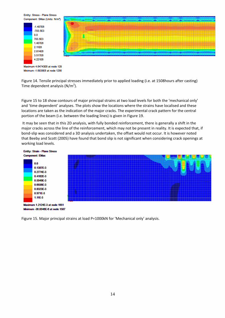
Figure 14. Tensile principal stresses immediately prior to applied loading (i.e. at 1508hours after casting) Time dependent analysis (N/m2).
Figure 15 to 18 show contours of major principal strains at two load levels for both the ‘mechanical only’ and ‘time dependent’ analyses. The plots show the locations where the strains have localised and these locations are taken as the indication of the major cracks. The experimental crack pattern for the central portion of the beam (i.e. between the loading lines) is given in Figure 19.
It may be seen that in this 2D analysis, with fully bonded reinforcement, there is generally a shift in the major cracks across the line of the reinforcement, which may not be present in reality. It is expected that, if bond‐slip was considered and a 3D analysis undertaken, the offset would not occur. It is however noted that Beeby and Scott (2005) have found that bond slip is not significant when considering crack openings at working load levels.
Figure 15. Major principal strains at load P=1000kN for ‘Mechanical only’ analysis.
15
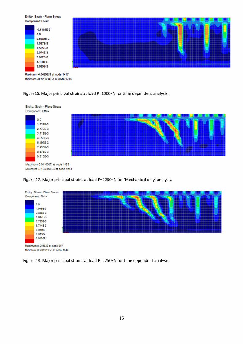
Figure16. Major principal strains at load P=1000kN for time dependent analysis.
Figure 17. Major principal strains at load P=2250kN for ‘Mechanical only’ analysis.
Figure 18. Major principal strains at load P=2250kN for time dependent analysis.
16
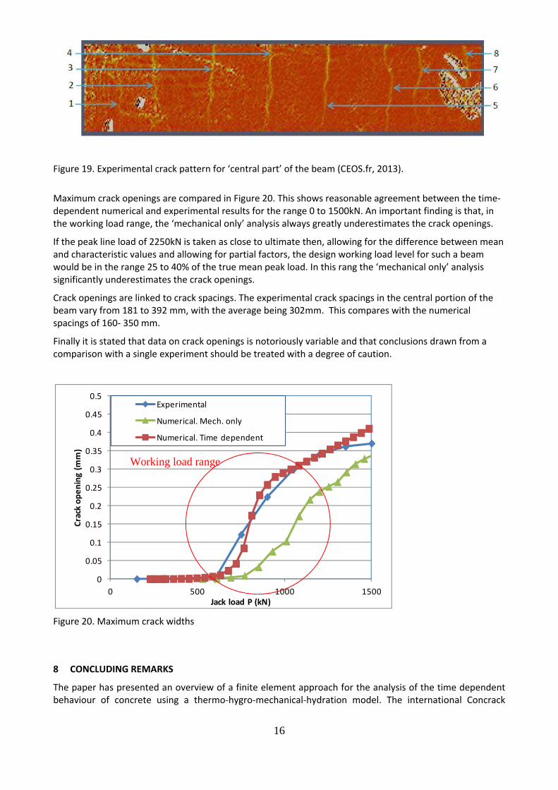
Figure 19. Experimental crack pattern for ‘central part’ of the beam (CEOS.fr, 2013).
Maximum crack openings are compared in Figure 20. This shows reasonable agreement between the time‐dependent numerical and experimental results for the range 0 to 1500kN. An important finding is that, in the working load range, the ‘mechanical only’ analysis always greatly underestimates the crack openings.
If the peak line load of 2250kN is taken as close to ultimate then, allowing for the difference between mean and characteristic values and allowing for partial factors, the design working load level for such a beam would be in the range 25 to 40% of the true mean peak load. In this rang the ‘mechanical only’ analysis significantly underestimates the crack openings.
Crack openings are linked to crack spacings. The experimental crack spacings in the central portion of the beam vary from 181 to 392 mm, with the average being 302mm. This compares with the numerical spacings of 160‐ 350 mm.
Finally it is stated that data on crack openings is notoriously variable and that conclusions drawn from a comparison with a single experiment should be treated with a degree of caution.
Figure 20. Maximum crack widths
8 CONCLUDING REMARKS
The paper has presented an overview of a finite element approach for the analysis of the time dependent behaviour of concrete using a thermo‐hygro‐mechanical‐hydration model. The international Concrack
0
0.05
0.1
0.15
0.2
0.25
0.3
0.35
0.4
0.45
0.5
0 500 1000 1500
Crack opening (m
m)
Jack load P (kN)
Experimental
Numerical. Mech. only
Numerical. Time dependent
Working load range
17
benchmark test RL1 has been considered with the present model, both with and without time dependent effects, with particular attention having been paid to the prediction of crack openings. The main conclusion from the work is that the crack openings predicted from a purely mechanical analysis in the working load level can be dramatically different from those predicted by a model that account for hydration, temperature variation and the time dependent effects of creep and shrinkage.
REFERENCES
Barr B, Hoseinian SB, Beygi MA (2003). Shrinkage of concrete stored in natural environments. Cement & Concrete Composites, 25, 19–29.
Bary B, Ranc G, Durand S, Carpentier O (2008). A coupled thermo‐hydro‐mechanical‐damage model for concrete subjected to moderate temperatures. International Journal of Heat and Mass Transfer, 51(11‐12), 2847‐2862.
Bazant ZP, Hauggaard AB, Baweja S and Ulm F‐J (1997). Microprestres‐solidification theory for concrete. Creep. I: Ageing and Drying Effects. ASCE Journal of Engineering Mechanics, Nov 1997, 1188‐1194.
Bažant, ZP, Oh, BH, (1983) Crack band theory for fracture in concrete. Materials and Structures 16, 155-177.
Beeby AW, Scott RH (2005). Cracking and deformation of axially reinforced members subjected to pure tension. Magazine of concrete research; 57(10):611‐621.
Benboudjema F, Torrenti JM, (2008). Early age behaviour of concrete nuclear containments. Nuclear Engineering and Design, 238(10), 2495‐2506.
CEOS.fr (2013). French National Research program, Comportement et Evaluation des Ouvrages Spéciaux, Fissuration – Retrait (Behaviour and Assessment of special reinforced concrete works – cracking & shrinkage), www.ceosfr.org, 2009‐2013.
De Schutter, G. (2002). Finite element simulation of thermal cracking in massive hardening concrete elements using degree of hydration based material laws. Computers and Structures, 80, 2035‐2042.
De Schutter, G and Taerwe, L (1997). Fracture energy of concrete at early ages. Materials and Structures 30, 67‐71.
Dufour F, Pijaudier‐Cabot G, Choinska M, Huerta A. (2008). Extraction of a crack opening from a continuous approach using regularized damage models. Computers and Concrete, 5 (4) 375‐388.
Gawin D, Pesavento F, Schrefler BA (2006). Hygro‐thermo‐chemo‐mechanical Modelling of Concrete at Early Ages and Beyond. Part I: Hydration and Hygro‐thermal Phenomena. International Journal for Numerical Methods in Engineering, 67, 299‐331.
Hilaire A., Benboudjema F., Darquennes A., Berthaud Y., Nahas G., Modeling basic creep in concrete at early‐age under compressive and tensile loading, Nuclear Engineering Design, Available online 31 August 2013
Jefferson AD (2003). Craft ‐ a plastic‐damage‐contact model for concrete. I. Model theory and thermodynamic considerations, International Journal of Solids and Structures, 40 (22), 5973‐5999.
Jefferson AD, Mihai IC and Lyons P (2014). An approach to modelling smoothed crack closure and aggregate interlock in the finite element analysis of concrete structures. Proceedings of EUROC, St Anton, 2014
Kovler K (1999). ‘A new look at the problem of drying creep of concrete under tension’. Journal of materials in civil engineering, ASCE, 84‐87.
Jennings HM, (2008). Refinements to colloid model of C‐S‐H in cement: CM‐II, Cement and Concrete Research, 38, 275‐289.
Lewis RW and Schrefler BA (1998). The finite element method in the static and dynamic deformation and consolidation of porous media. Wiley 1998.
18
EC2 (2008). Design of concrete structures — Part 1–1: General rules and rules for buildings. EN1992‐1‐1.
Oliver J, Huespe AE, Samaniego E. (2003). A study on finite elements for capturing strong discontinuities. International Journal for Numerical Methods in Engineering, 56, 2135–2161.
Østergaard, L., Lange, D.A., Altoubat, S.A., Stang, H., 2001. Tensile basic creep of early‐age concrete under constant load. Cement Concrete Res. 31, 1895–1899.
Rabczuk T, Belytschko T. 2007. A three‐dimensional large deformation meshfree method for arbitrary evolving cracks. Computational Methods in Applied Mechanics and Engineering, 196, 2777–2799.
Ranaivomanana N, Multon S, Turatsinze A, 2013. Basic creep of concrete undercompression, tension and bending. Constr. Build. Mater. 38, 173–180.
Schindler AK and Folliard KJ, (2005). Heat of hydration models for cementitious materials, ACI Journal, Feb 2005, 24‐33.
Rossi P, Tailhan J.‐L., Maou FL, Gaillet L, Martin E, 2012. Basic creep behavior ofconcretes investigation of the physical mechanisms by using acoustic emission. Cement Concrete Res. 42, 61–73.
Sellier A, Casaux‐Ginestet G, Buffo‐Lacarrière, L and Bourbon X (2013). Orthotropic damage coupled with localized crack reclosure processing. Engineering Fracture Mechanics, 97, Part 1 148–167, Part 2 168‐185.
Simo JC and Hughes TJR (1998). Computational Inelasticity. Springer
Tammo K, Lundgren K, Thelandersson S. (2009).Nonlinear analysis of crack widths in reinforced concrete. Magazine of Concrete Research, 61 (1), 23–34.
Tijssens MGA, Sluys BLJ, van der Giessen E. (2000) Numerical simulation of quasi‐brittle fracture and damaging cohesive surfaces. Eur J Mech A/solids, 19, 761–779.
van Genuchten MT (1980). A Closed‐form Equation for Predicting the Hydraulic Conductivity of Unsaturated Soils. Soil Sci. Soc. Am. J, 44, 892‐898
Wu HQ, Gilbert RI. (2009). Modeling short‐term tension stiffening in reinforced concrete prisms using a continuum‐based finite element model. Engineering Structures, 31(10), 2380‐2391.
Yi, S‐T, Kim, J‐K and Oh, TK, (2003). Effect of strength and age on the stress‐strain curves of concrete specimens. Cement and Concrete Research, 33, 1235‐1244.
19
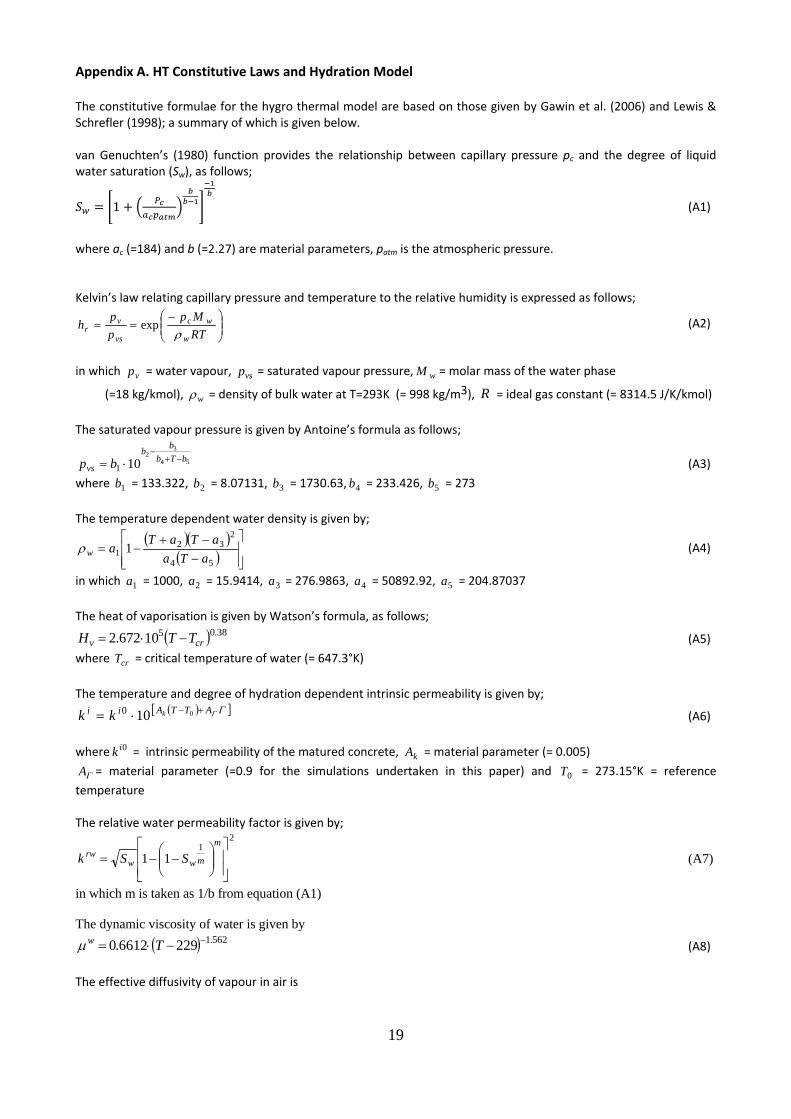
Appendix A. HT Constitutive Laws and Hydration Model The constitutive formulae for the hygro thermal model are based on those given by Gawin et al. (2006) and Lewis & Schrefler (1998); a summary of which is given below. van Genuchten’s (1980) function provides the relationship between capillary pressure pc and the degree of liquid water saturation (Sw), as follows;
1 (A1)
where ac (=184) and b (=2.27) are material parameters, patm is the atmospheric pressure. Kelvin’s law relating capillary pressure and temperature to the relative humidity is expressed as follows;
RT
Mp
p
ph
w
wc
vs
vr
exp (A2)
in which vp = water vapour, vsp = saturated vapour pressure, wM = molar mass of the water phase
(=18 kg/kmol), w = density of bulk water at T=293K (= 998 kg/m3), R = ideal gas constant (= 8314.5 J/K/kmol)
The saturated vapour pressure is given by Antoine’s formula as follows;
54
32
101bTb
bb
vs bp
(A3)
where 1b = 133.322, 2b = 8.07131, 3b = 1730.63, 4b = 233.426, 5b = 273
The temperature dependent water density is given by;
54
232
1 1aTa
aTaTaw (A4)
in which 1a = 1000, 2a = 15.9414, 3a = 276.9863, 4a = 50892.92, 5a = 204.87037
The heat of vaporisation is given by Watson’s formula, as follows;
38.0510672.2 crv TTH (A5)
where crT = critical temperature of water (= 647.3°K)
The temperature and degree of hydration dependent intrinsic permeability is given by;
ATTAii kkk 0100 (A6)
where 0ik = intrinsic permeability of the matured concrete, kA = material parameter (= 0.005)
A = material parameter (=0.9 for the simulations undertaken in this paper) and 0T = 273.15°K = reference
temperature The relative water permeability factor is given by;
21
11
m
mwwrw SSk (A7)
in which m is taken as 1/b from equation (A1) The dynamic viscosity of water is given by
562.12296612.0 Tw (A8)
The effective diffusivity of vapour in air is
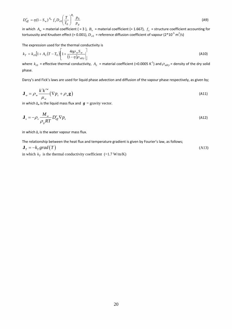
20
g
B
vsA
wveff p
p
T
TDfSD
v
w 0
00)1(
(A9)
in which wA = material coefficient ( = 3 ), vB = material coefficient (= 1.667), sf = structure coefficient accounting for
tortuousity and Knudsen effect (= 0.001), 0vD = reference diffusion coefficient of vapour (2*10‐5 m2/s)
The expression used for the thermal conductivity is
sdry
wwtT
STTAkk
1
411 00 (A10)
where 0tk = effective thermal conductivity, A = material coefficient (=0.0005 K‐1) and sdry = density of the dry solid
phase. Darcy’s and Fick’s laws are used for liquid phase advection and diffusion of the vapour phase respectively, as given by;
i rw
w w c ww
k kp
J g (A11)
in which Jw is the liquid mass flux and g = gravity vector.
vwv v eff v
g
MD p
RT
J (A12)
in which Jv is the water vapour mass flux. The relationship between the heat flux and temperature gradient is given by Fourier’s law, as follows;
T Tk grad T J (A13)
in which Tk is the thermal conductivity coefficient (=1.7 W/m/K)
21
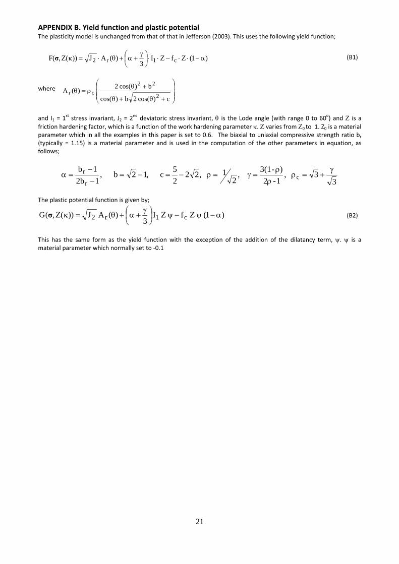
APPENDIX B. Yield function and plastic potential The plasticity model is unchanged from that of that in Jefferson (2003). This uses the following yield function;
)1(fI3
)(AJ))(,(F c1r2
σ (B1)
where
c)cos( 2b)cos(
b)cos( 2 )(A
2
22
cr
and I1 = 1st stress invariant, J2 = 2
nd deviatoric stress invariant, is the Lode angle (with range 0 to 60o) and is a friction hardening factor, which is a function of the work hardening parameter . varies from 0 to 1. Z0 is a material parameter which in all the examples in this paper is set to 0.6. The biaxial to uniaxial compressive strength ratio br (typically = 1.15) is a material parameter and is used in the computation of the other parameters in equation, as follows;
33 ,
1-2
)-3(1 ,
21 ,22
2
5c ,12b ,
1b2
1bc
r
r
The plastic potential function is given by;
)1( f I 3
)(A J))(,(G c1r2
σ (B2)
This has the same form as the yield function with the exception of the addition of the dilatancy term, . is a material parameter which normally set to ‐0.1

22