finding an initial basic feasible solution for dea models with an application on bank industry
TRANSCRIPT
Comput EconDOI 10.1007/s10614-014-9423-1
Finding an Initial Basic Feasible Solution for DEAModels with an Application on Bank Industry
Mehdi Toloo · Atefeh Masoumzadeh · Mona Barat
Accepted: 29 January 2014© Springer Science+Business Media New York 2014
Abstract Nowadays, algorithms and computer programs, which are going to speedup, short time to run and less memory to occupy have special importance. Towardthese ends, researchers have always regarded suitable strategies and algorithms withthe least computations. Since linear programming (LP) has been introduced, interestin it spreads rapidly among scientists. To solve an LP, the simplex method has beendeveloped and since then many researchers have contributed to the extension andprogression of LP and obviously simplex method. A vast literature has been grownout of this original method in mathematical theory, new algorithms, and applied nature.Solving an LP via simplex method needs an initial basic feasible solution (IBFS), butin many situations such a solution is not readily available so artificial variables willbe resorted. These artificial variables must be dropped to zero, if possible. There aretwo main methods that can be used to eliminate the artificial variables: two-phasemethod and Big-M method. Data envelopment analysis (DEA) applies individual LPfor evaluating performance of decision making units, consequently, to solve theseLPs an IBFS must be on hand. The main contribution of this paper is to introduce aclosed form of IBFS for conventional DEA models, which helps us not to deal withartificial variables directly. We apply the proposed form to a real-data set to illustrate
M. Toloo (B)Department of Business Administration, Faculty of Economics,Technical University of Ostrava, Ostrava, Czech Republice-mail: [email protected]; [email protected]
A. MasoumzadehDepartment of Mathematics, Islamic Azad University, Central Tehran Branch,Tehran, Iran
M. BaratDepartment of Mathematics, Islamic Azad University, Mahshahr Branch,Mahshahr, Iran
123
M. Toloo et al.
the applicability of the new approach. The results of this study indicate that using theclosed form of IBFS can reduce at least 50 % of the whole computations.
Keywords Data envelopment analysis · Initial basic feasible solution ·Artificial variable · Two-phase method
1 Introduction
Speed and accuracy in calculation have a great importance in modern and complexworld. On the other hand, developed algorithms, which meet the minimum error incalculation, squandering less time of central processing unit (CPU), and the lowestcash memory occupation have always been considered. One of the subjects that hasbeen attracted attentions of many mathematicians, statisticians, and engineers is linearprogramming (LP). Simplex method, which was introduced by George B. Dantzig in1949, is a well-known method for solving LPs. While this algorithm performs fully insmall or medium sized problems, in the worst case the algorithm tends to exponentialcomplexity in its performance, so finding a faster way for solving LPs that lessensthe process of the simplex method is a critical debate. As mentioned earlier, initialbasic feasible solution (IBFS) plays an important role in commencing the simplexmethod. To start the simplex method, a feasible basis B must be available. In somesituations the problem can be initiated by a very simple basis, namely the identity,but in many cases such a basis is not easily available. This case takes place when theconstraint matrix A has no identity sub-matrix, therefore we shall resort to artificialvariables to use the simplex method. However, eliminating these artificial variables isnecessary to obtain a BFS for the main problem. There are various methods to get ridof these unwanted guests; two main approaches are two-phase and big-M methods.Big-M method involves a parameter that must be selected properly. In fact, findinga proper value for the parameter is still an open problem. On the other hand, theBig-M method may lead to the round-off computational error for a large value ofM . Hence, commercial software prefers to utilize the two-phase method instead ofthe Big-M method. As we will see in the next paragraph data envelopment analysis(DEA) models are a sort of LPs so to solve these models an IBFS is necessary. In thispaper, a two-phase based approach is introduced to achieve an IBFS in DEA models.
Data envelopment analysis that was originated by Charnes et al. (1978), CCR model,and extended by Banker et al. (1984), BCC model, is a non-parametric LP approach toevaluate the performance of decision making units (DMUs) with multiple inputs andmultiple outputs. Notwithstanding some other evaluating methods that choose a prior(fixed) set of weights (multipliers) for inputs and outputs, DEA drives the weightsdirectly from the data in a manner that assigns a best set of them to each DMU thatmay vary from one DMU to another. To measure the relative efficiency of each DMUby DEA models, one optimization problem should be run. Knowing that DEA modelsare always feasible, their feasible regions involve at least one BFS, hence the simplexmethod should be applied to solve the efficiency problem. As mentioned earlier forsolving an LP problem (here a kind of DEA model) an identity sub-matrix must be onhand. If the constraint matrix A in a DEA model has no identity sub-matrix, artificial
123

Initial Basic Feasible Solution for DEA Models
variables will be resorted. Regarding to the constraints of these models, for exampleconsider the CCR multiplier form, to start the simplex method one artificial variableis needed for each input and output and also an artificial variable for the normalizationconstraint. If we apply two-phase method to eliminate the artificial variables, we willhave a BFS at the end of phase I (note that DEA models are always feasible). It shouldbe kept in mind that DEA models have degeneracy; hence more iterations are coveredto find a BFS. Furthermore, increasing number of DMUs leads to the exponentiallyincreasing in number of iterations and computations. This seems awkward and ofcourse time consuming. In this paper we explore a way that decreases the number ofiterations needed in finding a BFS. We introduce a closed form of IBFS for the CCRmodel and hence, an IBFS is on hand without the necessity of solving any LP.
The rest of this paper is structured as follows: Sect. 2 reviews one of the most basicDEA models. In Sect. 3, a closed form of IBFS to some conventional DEA models isintroduced. An application of the proposed approach is shown in Sect. 4, as a resultwe see that the less number of iterations is perfectly depicted. The paper ends up withconclusion and remarks section.
2 The CCR Model
Charnes et al. (1978) proposed DEA approach, the CCR model, which is an applicablemethodology for determining the relative efficiencies of DMUs with multiple inputsand outputs. Suppose we wish to evaluate the efficiencies of n homogeneous DMUs.Each DMU j ( j = 1, . . . , n) produces s different outputs y j = (y j1, . . . , y js), usingm different inputs x j = (x j1, . . . , x jm). More compactly, we can arrange input andoutput data in the matrix form, X ∈ Rn×m and Y ∈ Rn×s , respectively. It is alsoassumed that inputs and outputs levels are non-negative. The multiplier form of theCCR model is as follows,
max yous.t. xov = 1
Yu − Xv ≤ 0n
u ≥ εs
v ≥ εm,
(1)
where v ∈ Rm and u ∈ Rs are the inputs and outputs weight column vectors respec-tively, 0n refers to origin in Rn space, and εl = (ε, ε, . . . , ε)t ∈ Rl where ε is anon-Archimedean infinitesimal for obtaining nonzero optimal weights.
Ali and Seiford (1993) proposed a theorem to get an upper bound for the mentionedepsilon. They showed that the envelopment forms of the CCR model for all DMUsare bounded if
ε <1
minj=1,...,n
{∑mi=1 x ji
} .
Mehrabian et al. (2000) demonstrated, by a counterexample, that the above upperbound of epsilon is not always true. They proposed a method for finding the assur-
123

M. Toloo et al.
ance interval for epsilon. It was proved that the following LP could be applied fordetermining the non-Archimedean ε in the assurance interval(0, ε∗],
max ε
s.t. x j v ≤ 1 j = 1, . . . , ny j u − x j v ≤ 0 j = 1, . . . , nu − εs ≥ 0s
v − εm ≥ 0m .
(2)
Let ε∗ be the optimal value of model (2), then model (1) is always feasible for anyε ∈ (0, ε∗].
Amin and Toloo (2004) claimed that an assurance value could be determined by apolynomial-time algorithm, without the necessity of solving any LP,
Algorithm Epsilon:
BeginM := 1/max
{x j 1m : j = 1, . . . , n
};N := min
{(x j 1m
)/(y j 1s
) : j = 1, . . . , n} ;
ε := min {M, N M} ;End
where 1m = (1, 1, . . . , 1)t ∈ Rm . Obviously, this algorithm is more useful thanprevious LP model, especially when computational issues and complexity analysisare at focus.
3 Closed Form of IBFS
The simplex method starts with an IBFS and moves toward an improved BFS, untilthe optimal point is reached or unboundedness will be achieved. However, in order toinitialize the simplex method a feasible basis B must be available. In many situations,finding an IBFS is not easily available because after manipulating the constraints andintroducing slack variables the technological coefficient matrix has no identity sub-matrix. The same difficulty may happen to the CCR model while we try to solve it viasimplex method. After introducing d ∈ Rn, s+ ∈ Rs and s− ∈ Rm to the multiplierform of the CCR model and identify them as “slacks”, the standard form of model (1)can be written as follows,
max yous.t. xov = 1
Yu − Xv + d = 0n
u − s+ = εs
v − s− = εm
u ≥ 0s, v ≥ 0m
d ≥ 0n, s+ ≥ 0s, s− ≥ 0m .
(3)
123
Initial Basic Feasible Solution for DEA Models
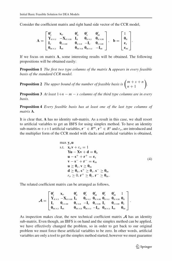
Consider the coefficient matrix and right hand side vector of the CCR model,
A =
⎡
⎢⎢⎣
0ts xo 0t
nYn×s −Xn×m In
Is 0s×m 0s×n
0m×s Im 0m×n
0ts 0t
m0n×s 0n×m
−Is 0s×m
0m×s −Im
⎤
⎥⎥⎦ , b =
⎡
⎢⎢⎣
10nεsεm
⎤
⎥⎥⎦.
If we focus on matrix A, some interesting results will be obtained. The followingpropositions will be obtained easily:
Proposition 1 The first two type columns of the matrix A appears in every feasiblebasis of the standard CCR model.
Proposition 2 The upper bound of the number of feasible basis is
(m + s + nn + 1
).
Proposition 3 At least 1+n − m − s columns of the third type columns are in everybasis.
Proposition 4 Every feasible basis has at least one of the last type columns ofmatrix A.
It is clear that, A has no identity sub-matrix. As a result in this case, we shall resortto artificial variables to get an IBFS for using simplex method. To have an identitysub-matrix m +s+1 artificial variables, r− ∈ Rm, r+ ∈ Rs and ro, are introduced andthe multiplier form of the CCR model with slacks and artificial variables is obtained,
max yous.t. xov + ro = 1
Yu − Xv + d = 0n
u − s+ + r+ = εs
v − s− + r− = εm
u ≥ 0s, v ≥ 0m
d ≥ 0n, s+ ≥ 0s, s− ≥ 0m
ro ≥ 0, r+ ≥ 0s, r− ≥ 0m .
(4)
The related coefficient matrix can be arranged as follows,
A =
⎡
⎢⎢⎣
0ts xo 0t
n 0ts 0t
m 0ts 0t
m 1Yn×s −Xn×m In 0n×s 0n×m 0n×s 0n×m 0n
Is 0s×m 0s×n −Is 0s×m Is 0s×m 0s
0m×s Im 0m×n 0m×s −Im 0m×s Im 0m
⎤
⎥⎥⎦ .
As inspection makes clear, the new technical coefficient matrix A has an identitysub-matrix. Even though, an IBFS is on hand and the simplex method can be applied,we have effectively changed the problem, so in order to get back to our originalproblem we must force these artificial variables to be zero. In other words, artificialvariables are only a tool to get the simplex method started; however we must guarantee
123
M. Toloo et al.
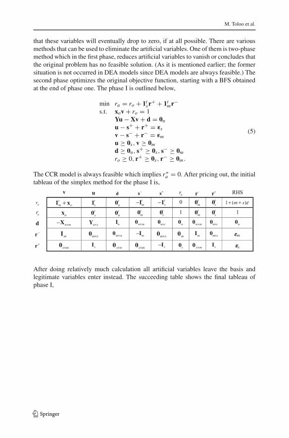
that these variables will eventually drop to zero, if at all possible. There are variousmethods that can be used to eliminate the artificial variables. One of them is two-phasemethod which in the first phase, reduces artificial variables to vanish or concludes thatthe original problem has no feasible solution. (As it is mentioned earlier; the formersituation is not occurred in DEA models since DEA models are always feasible.) Thesecond phase optimizes the original objective function, starting with a BFS obtainedat the end of phase one. The phase I is outlined below,
min ra = ro + 1tsr+ + 1t
mr−s.t. xov + ro = 1
Yu − Xv + d = 0n
u − s+ + r+ = εs
v − s− + r− = εm
u ≥ 0s, v ≥ 0m
d ≥ 0n, s+ ≥ 0s, s− ≥ 0m
ro ≥ 0, r+ ≥ 0s, r− ≥ 0m .
(5)
The CCR model is always feasible which implies r∗a = 0. After pricing out, the initial
tableau of the simplex method for the phase I is,
After doing relatively much calculation all artificial variables leave the basis andlegitimate variables enter instead. The succeeding table shows the final tableau ofphase I,
123

Initial Basic Feasible Solution for DEA Models
123

M. Toloo et al.
At the end of phase I we have m + s + n + 1 basic variables, which can be used tostart phase II. According to the last tableau, a closed form of an IBFS for the multiplierform of the CCR model can be written easily. More precisely, a closed form of an IBFSfor a DMU, namely DMUo, is,
s−1 = 1−xoεm
xo1
v1 = ε + s−1
vi = ε i = 2, . . . , mur = ε r = 1, . . . , sd j = ε(x j 1m − y j 1s) + x j1s−
1 j = 1, . . . , n
and all other variables are non-basic.An IBFS for the envelopment of the CCR model can be obtained in a similar way.
Since the computation for this form of the CCR model is straightforward we suspendit till the Appendix part.
Now we switch our attention to the degeneracy of DEA models. According to thedegeneracy of the CCR model when a degenerate pivot occurs in the simplex method,we may shift from one basis to another which represents the same extreme point. Thismay cause performing more iterations and hence more computation. In this sectionwe have just shown that an IBFS can be suggested to the CCR model. It means thatwithout solving phase I (for all n DMUs) to find an IBFS, the CCR model is solved.
Like the CCR, the BCC model also needs an IBFS to start. The very similarity ofthe CCR and the BCC models (with this perspective) allows us to use the mentionedmethod to find an IBFS for the BCC, as well.
In the following section we apply the new proposed method to a numerical exampleand also a real data set from a bank, in the context of the above development.
4 Applications
In this section we examine the validity of the new approach with a numerical exampleand a real case. We see that using IBFS significantly decreases the number of iterationsand operations.
4.1 Numerical Example
In this part, we apply the procedure introduced in this paper to the famous data set ofCooper et al. (2007). There are 12 hospitals with two inputs (the number of doctors andnurses) and two outputs (the number of outpatients and inpatients). The input/outputdata are summarized in Table 1.
Model (5) was applied to the data of Table 1. The coefficient matrix of the standardmultiplier form of the CCR model for evaluating hospital A is shown below,
123

Initial Basic Feasible Solution for DEA Models
Table 1 The data of 12 hospitals
Hospital A B C D E F G H I J K L
Doctors 20 19 25 27 22 55 33 31 30 50 53 38
Nurses 151 131 160 168 158 255 235 206 244 268 306 284
Outpatients 100 150 160 180 94 230 220 152 190 250 260 250
Inpatients 90 50 55 72 66 90 88 80 100 100 147 120
A =
⎡
⎢⎢⎢⎢⎢⎢⎢⎢⎢⎢⎢⎢⎢⎢⎢⎢⎢⎢⎢⎢⎢⎢⎢⎢⎢⎢⎢⎢⎣
20 151 0 0 0 0 0 0 0 0 0 0 0 0 0 0 0 0 0 0−20 −151 100 90 1 0 0 0 0 0 0 0 0 0 0 0 0 0 0 0−19 −131 150 50 0 1 0 0 0 0 0 0 0 0 0 0 0 0 0 0−25 −160 160 55 0 0 1 0 0 0 0 0 0 0 0 0 0 0 0 0−27 −168 180 72 0 0 0 1 0 0 0 0 0 0 0 0 0 0 0 0−22 −158 94 66 0 0 0 0 1 0 0 0 0 0 0 0 0 0 0 0−55 −255 230 90 0 0 0 0 0 1 0 0 0 0 0 0 0 0 0 0−33 −235 220 88 0 0 0 0 0 0 1 0 0 0 0 0 0 0 0 0−31 −206 152 80 0 0 0 0 0 0 0 1 0 0 0 0 0 0 0 0−30 −244 190 100 0 0 0 0 0 0 0 0 1 0 0 0 0 0 0 0−50 −268 250 100 0 0 0 0 0 0 0 0 0 1 0 0 0 0 0 0−53 −306 260 147 0 0 0 0 0 0 0 0 0 0 1 0 0 0 0 0−38 −284 250 120 0 0 0 0 0 0 0 0 0 0 0 1 0 0 0 0
1 0 0 0 0 0 0 0 0 0 0 0 0 0 0 0 −1 0 0 00 1 0 0 0 0 0 0 0 0 0 0 0 0 0 0 0 −1 0 00 0 1 0 0 0 0 0 0 0 0 0 0 0 0 0 0 0 −1 00 0 0 1 0 0 0 0 0 0 0 0 0 0 0 0 0 0 0 −1
⎤
⎥⎥⎥⎥⎥⎥⎥⎥⎥⎥⎥⎥⎥⎥⎥⎥⎥⎥⎥⎥⎥⎥⎥⎥⎥⎥⎥⎥⎦
Here we explain how the IBFS is reached for hospital A. For other hospitals theprocedure is the same, therefore we do not mention the calculation.
Via the algorithm of epsilon we have,
M = 1
359= 0.0027
N = 0.75
ε = min{M, M N }= min{0.0027, 0.002089} = 0.002089.
By imposing this ε to model (1) and solving the resulting model, the closed form ofIBFS can be obtained as follows,
s−1 = 0.03000,
v1 = 0.03209, v2 = 0.00209
u1 = 0.00209, u2 = 0.00209
d1 = 0.56031, d2 = 0.46555, d3 = 0.68733, d4 = 0.69092
d5 = 0.70178, d6 = 1.62911, d7 = 0.90644, d8 = 0.94044
d9 = 0.86657, d10 = 1.43315, d11 = 1.48972, d12 = 1.03973
123

M. Toloo et al.
Table 2 The data for bank branches
DMU Employees Current cost Over due debt Deposits Incomes Loans
Branch 1 32 167 446,698 515,578 40,254 1,277,833
Branch 2 19 2,026 22,585 187,679 13,304 102,808
Branch 3 14 1,857 12,830 150,026 6,783 106,734
Branch 4 5 1,674 161 88,358 756 14,628
Branch 5 18 1,953 21,035 124,349 2,521 75,509
Branch 6 18 1,753 39,525 127,370 5,252 149,860
Branch 7 16 1,989 9,632 95,288 4,690 55,757
Branch 8 17 1,285 13,955 89,304 5,766 84,631
Branch 9 9 1,838 7,153 160,138 8,395 102,353
Branch 10 13 2,011 7,806 148,755 2,697 38,375
Branch 11 8 1,608 3,762 14,0413 3,665 20,398
Branch 12 11 1,914 17,861 72,149 3,153 57,537
Branch 13 17 1,839 11,796 89,781 2,673 51,114
Branch 16 14 1,430 15,118 77,031 1,881 43,487
Branch 17 14 1,409 11,947 75,923 2,261 41,442
Branch 14 7 1,511 14,867 42,654 2,354 52,485
Branch 15 12 1,962 10,383 97,812 4,782 67,298
Branch 18 9 1,478 16,423 47,763 2,028 43,262
Branch 19 5 1,500 3,772 45,732 756 14,237
Branch 20 6 1,153 31,647 55,222 863 41,062
Branch 21 6 2,429 4,986 53,323 2,469 37,418
Branch 22 8 2,076 18,700 69,734 2,433 57,883
Branch 23 9 1,652 15,773 49,153 2,364 47,139
Branch 24 8 2,100 7,705 92,365 5,663 55,543
Branch 25 7 1,944 3,752 64,235 1,361 22,347
Branch 26 9 1,528 4,875 89,104 2,681 45,717
Branch 27 7 1,728 30,614 42,012 2,814 73,925
Branch 28 7 2,008 4,584 69,360 2,240 27,246
Branch 29 7 1,670 4,977 51,438 2,293 26,531
Branch 30 6 1,578 4,495 39,948 1,151 20,223
Branch 31 7 1,514 9,464 154,284 1,518 43,928
Branch 32 7 1,594 4,953 61,101 1,855 25,718
Branch 33 8 2,079 5,405 81,544 1,711 27,985
Branch 34 9 1,555 8,109 79,046 8,085 58,355
Branch 35 5 2,051 5,185 47,876 648 14,055
Branch 36 7 1,543 9,235 71,606 4,289 68,341
Branch 37 8 2,363 728 124,146 8,563 54,541
Branch 38 6 1,881 1,577 77,868 1,965 33,838
Branch 39 5 1,537 3,534 58,696 2,248 28,476
123

Initial Basic Feasible Solution for DEA Models
Table 2 continued
DMU Employees Current cost Over due debt Deposits Incomes Loans
Branch 40 9 1,609 6,881 67,892 4,475 66,061
Branch 41 5 1,702 19,500 34,275 2,693 51,241
Branch 42 6 1,861 8,204 40,233 1,144 31,420
Branch 43 6 1,586 15,788 36,597 899 31,072
Branch 48 7 1,630 22,078 28,604 4,500 80,208
Branch 53 5 1,986 4,280 71,220 2,009 42,410
Branch 44 5 2,174 7,356 38,443 1,762 36,710
Branch 45 6 2,028 4,663 46,110 940 16,732
Branch 46 5 1,606 1,047 34,692 632 11,235
Branch 47 6 1,560 4,797 39,740 838 20,687
Branch 49 4 1,632 2,777 34,905 470 10,612
Branch 50 5 1,599 8,554 24,805 867 22,902
Table 3 The number of iterations
Groups No. of DMUs No. of iterations inphase I
No. of iterations inphase II
Total iterations Percent ofreduction
1 5 40 20 60 66.6
2 10 80 70 150 53.3
3 20 180 180 360 50
4 30 330 300 630 55
5 50 600 600 1,200 50
Table 4 The number of multiplications and additions
Groups No. ofDMUs
No. of adds ineach iterations
No. of multiplicationsin each iterations
Total reducedadds
Total reducedmultiplications
Totalreductions
1 5 156 169 6,240 6,760 13,000
2 10 221 234 17,680 18,720 36,400
3 20 351 364 63,180 65,520 128,700
4 30 481 494 158,730 163,020 321,750
5 50 741 754 444,600 452,400 897,000
and all other variables are non-basic. An IBFS for each of other DMUs can be obtainedin a similar way.
4.2 Real-World Example
We examine the new approach in a real data set involves 50 branches of the largestprivate bank in Iran. It is noted that for purposes of our analysis, we use the three inputs,employees, current cost, and overdue debt. Outputs consist of deposits, incomes, andloans. We should mention that employees consists of managers and clerks of each
123

M. Toloo et al.
branches, current cost, consists of the cost of administrative, personal and energy,and loans consist of real estate, commercial and industrial loans that bank gives to itscostumer. The data for bank branches are displayed in Table 2.
To show that the new approach decreases the number of iterations and hence cal-culation, we apply the proposed approach to the data of Table 2. We consider fivegroups in the following manner: groups 1–5 consist of 5, 10, 20, 30, and 50 DMUs,respectively. Then we run the CCR model for each group and compare the amountof calculation by and without using closed form. For instance, if we apply the CCRmodel to the group 1 with 5 DMUs, we need 60 iterations (40 iterations for phase Iand 20 iterations for phase II), but the closed form permits us omit the phase I, andhence 66 % of iterations will decrease.
The number of iterations in phase I and phase II for evaluating the relative efficiencyof each group is summarized in Table 3. The 2nd and 3rd columns in this table presentthe number of iterations in phase I and phase II. The 4th column has shown the totaliterations for evaluating the relative efficiency of each group. The last column showsthat at least 50 % of computational is reduced by using the new approach.
According to Bazaraa et al. (2010), the simplex method for the CCR model inphase I empirically requires (m + s + n + 1) to 3 (m + s + n + 1) iterations, and ineach iteration it needs 2(n + m + s + 1)(m + s) + n + 3m + 3s + 2 multiplicationsand (n + m + s + 1)(2m + 2s + 1) additions. To emphasize the applicability of theproposed method we calculate the number of operations per iteration that must bedone for each group of DMUs that mentioned before. In Table 4 we see the numberof multiplications and additions required during each iteration of phase I. It is easilyunderstood that by using the proposed closed form of IBFS and omitting the phase I,significant number of iterations is reduced.
5 Conclusion
This paper has presented a closed form of an IBFS for the CCR model. Because ofthe very similarity of the CCR and BCC models, an IBFS for the BCC model canbe obtained in a similar way. By applying this approach, we solve the phase I of thetwo-phase method for a DMU, namely DMUo, and find a closed form of IBFS to startphase II. This closed form of the IBFS can be used for each DMU. According to thefact that conventional DEA models require at least n+m +s +1 iterations to achieve aBFS for starting the simplex method and due to the inherent likelihood of degeneracyin DEA LP problems, we should do relatively large number of iterations for findingan IBFS. What is remarkable here is that by using this closed form, it is not requiredto solve phase I anymore and by omitting this phase significant number of iterationsis disappeared, on the operations aspects 2(n + m + s + 1)(m + s)+ n + 3m + 3s + 2number of multiplications and (n + m + s + 1)(2m + 2s + 1) number of additionswill be reduced.
To show the applicability of this modification we apply this approach in two appliedsettings, a numerical example and a real-world example. Results indicate that usingthis IBFS decreases at least 50 % of computations. Similar research can be repeated fordealing with other DEA models such as Additive and slacks-based measure models.
123
Initial Basic Feasible Solution for DEA Models
Acknowledgments The research was supported by the Czech Science Foundation (GACR project 14-31593S) and through European Social Fund within the project CZ.1.07/2.3.00/20.0296.
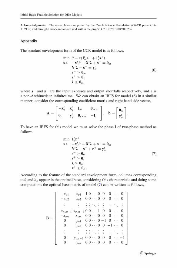
Appendix
The standard envelopment form of the CCR model is as follows,
min θ − ε(1tms− + 1t
ss+)
s.t. −xtoθ + Xtλ + s− = 0m
Ytλ − s+ = yto
s− ≥ 0m
s+ ≥ 0s
λ ≥ 0n,
(6)
where s− and s+ are the input excesses and output shortfalls respectively, and ε isa non-Archimedean infinitesimal. We can obtain an IBFS for model (6) in a similarmanner; consider the corresponding coefficient matrix and right hand side vector,
A =⎡
⎣−xt
o xtj Im 0m×s
0s ytj 0s×m −Is
⎤
⎦ , b =[
0m
yto
]
.
To have an IBFS for this model we must solve the phase I of two-phase method asfollows:
min 1tsr+
s.t. −xtoθ + Xtλ + s− = 0m
Ytλ − s+ + r+ = yto
s− ≥ 0m
s+ ≥ 0s
λ ≥ 0n
r+ ≥ 0s .
(7)
According to the feature of the standard envelopment form, columns correspondingto θ and λo appear in the optimal base, considering this characteristic and doing somecomputations the optimal base matrix of model (7) can be written as follows,
B =
⎡
⎢⎢⎢⎢⎢⎢⎢⎢⎢⎢⎢⎢⎢⎢⎢⎢⎣
−xo1 xo1 1 0 · · · 0 0 0 · · · 0−xo2 xo2 0 0 · · · 0 0 0 · · · 0
......
......
. . ....
......
. . ....
−xo,m−1 xo,m−1 0 0 · · · 1 0 0 · · · 0−xom xom 0 0 · · · 0 0 0 · · · 0
0 yo1 0 0 · · · 0 −1 0 · · · 00 yo2 0 0 · · · 0 0 −1 · · · 0...
......
.... . .
......
.... . .
...
0 yo,s−1 0 0 · · · 0 0 0 · · · −10 yos 0 0 · · · 0 0 0 · · · 0
⎤
⎥⎥⎥⎥⎥⎥⎥⎥⎥⎥⎥⎥⎥⎥⎥⎥⎦
123

M. Toloo et al.
The closed form of B−1 can be calculated as,
B−1 =
⎡
⎢⎢⎢⎢⎢⎢⎢⎢⎢⎢⎢⎢⎢⎢⎢⎢⎢⎢⎣
0 0 . . . 0 − 1xom
0 0 · · · 0 1yos
0 0 · · · 0 0 0 0 · · · 0 1yos
1 0 · · · 0 − xo1xom
0 0 · · · 0 00 1 · · · 0 − xo2
xom0 0 · · · 0 0
......
. . ....
......
.... . .
......
0 0 · · · 1 − xo,m−1xom
0 0 · · · 0 00 0 · · · 0 0 −1 0 · · · 0 yo1
yos
0 0 · · · 0 0 0 −1 · · · 0 yo2yso
......
. . ....
......
.... . .
......
0 0 · · · 0 0 0 0 · · · −1 yo,s−1yos
⎤
⎥⎥⎥⎥⎥⎥⎥⎥⎥⎥⎥⎥⎥⎥⎥⎥⎥⎥⎦
Hence, the following optimal solution will be achieved:
θ = 1λo = 1s−
i = 0 i = 1, . . . , m − 1s+r = 0 r = 1, . . . , s − 1
and all other variables are non-basic. Indeed, this solution is a degenerate BFS of orderm+s −2 and consequently we expect that the significant number of iterations in phaseI will be saved by applying the proposed IBFS.
Now, we have a closed form of an IBFS for the envelopment form of the CCRmodel to start phase II without solving phase I.
References
Ali, A., & Seiford, L. M. (1993). Computational accuracy and infinitesimal in data envelopment analysis.INFOR, 31, 290–297.
Amin, G. R., & Toloo, M. (2004). A polynomial-time algorithm for finding ε in DEA models. Computer& Operation Research, 31, 803–805.
Banker, R. D., Charnes, A., & Cooper, W. W. (1984). Models for estimation of technical and scale ineffi-ciencies in data envelopment analysis. Management Science, 30, 1078–1092.
Bazaraa, M. S., Jarvis, J. J., & Sherali, H. D. (2010). Linear programming and network flows (4th ed.).New York: Wiley.
Charnes, A., & Cooper, W. W. (1992). Programming with linear fractional. Naval Research LogisticsQuarterly, 15, 333–334.
Charnes, A., Cooper, W. W., & Rhodes, E. (1978). Measuring the efficiency of decision making units.European Journal of Operational Research, 2, 429–444.
Cooper, W. W., Seiford, L. M., & Tone, K. (2007). Introduction to data envelopment analysis and its useswith DEA-solver software and references (2nd ed.). New York: Springer.
Mehrabian, S., Jahanshahloo, G. R., Alirezaee, M. R., & Amin, G. R. (2000). An assurance interval for thenon-Archimedean epsilon in DEA models. Operations Research, 48, 3444–3447.
123