Financial Intermediary Capital∗

Adriano A. RampiniDuke University

S. ViswanathanDuke University

First draft: July 2010This draft: March 2012

Abstract

We propose a dynamic theory of financial intermediaries as collateralizationspecialists that are better able to collateralize claims than households. Interme-diaries require capital as they can borrow against their loans only to the extentthat households themselves can collateralize the assets backing the loans. The networth of financial intermediaries and the corporate sector are both state variablesaffecting the spread between intermediated and direct finance and the dynamics ofreal economic activity, such as investment, and financing. The accumulation of networth of intermediaries is slow relative to that of the corporate sector. A creditcrunch has persistent real effects and can result in a delayed or stalled recovery. Weprovide sufficient conditions for the comovement of the marginal value of firm andintermediary capital.

Keywords: Collateral; Financial intermediation; Financial constraints; Investment

∗We thank Nittai Bergman, Doug Diamond, Emmanuel Farhi, Itay Goldstein, Bengt Holmstrom,Nobu Kiyotaki, David Martinez-Miera, Alexei Tchistyi, and seminar participants at the IMF, the MITtheory lunch, Boston University, the Federal Reserve Bank of New York, the Stanford University macrolunch, the Federal Reserve Bank of Richmond, the 2010 SED Annual Meeting, the 2010 Tel Aviv Univer-sity Finance Conference, the 2011 Jackson Hole Finance Conference, the 2011 FIRS Annual Conference,the 2011 WFA Annual Meeting, the 2011 CEPR European Summer Symposium in Financial Markets,the 2011 FARFE Conference, and the 2012 AEA Conference for helpful comments. This paper subsumesthe results on financial intermediation in our 2007 paper “Collateral, financial intermediation, and thedistribution of debt capacity,” which is now titled “Collateral, risk management, and the distribution ofdebt capacity” (Rampini and Viswanathan (2010)). Address: Duke University, Fuqua School of Business,100 Fuqua Drive, Durham, NC, 27708. Rampini: Phone: (919) 660-7797. Email: rampini@duke.edu.Viswanathan: Phone: (919) 660-7784. Email: viswanat@duke.edu.

1 Introduction

The capitalization of financial intermediaries is arguably critical for economic fluctua-

tions and growth. We provide a dynamic model in which financial intermediaries are

collateralization specialists and firms need to collateralize promises to pay with tangible

assets. Financial intermediaries are modeled as lenders that are able to collateralize a

larger fraction of tangible assets than households who lend to firms directly, that is, are

better able to enforce their claims. Financial intermediaries require net worth as their

ability to refinance their collateralized loans from households is limited, as they, too,

need to collateralize their promises. The net worth of financial intermediaries is hence

a state variable and affects the dynamics of the economy. Importantly, both firm and

intermediary net worth play a role in our model and jointly affect the dynamics of firm

investment, financing, and loan spreads. Spreads on intermediated finance are high when

both firms and financial intermediaries are poorly capitalized and in particular when in-

termediaries are moreover poorly capitalized relative to firms. One of our main results

is that intermediaries accumulate net worth more slowly than the corporate sector. This

has important implications for economic dynamics. For example, a credit crunch, that is,

a drop in intermediary net worth, has persistent real effects and can result in a delayed

or stalled recovery.

In our model, firms can raise financing either from households or from financial inter-

mediaries. Firms have to collateralize their promises to pay due to limited enforcement.1

Both households and intermediaries extend collateralized loans, but financial intermedi-

aries are better able to collateralize promises and hence are able to extend more financing

per unit of tangible assets collateralizing their loans. Financial intermediaries in turn are

able to borrow against their loans, but only to the extent that other lenders themselves

can collateralize the assets backing the loans. Intermediaries thus need to finance the ad-

ditional amount that they are able to lend out of their own net worth. Since intermediary

net worth is limited, intermediated finance commands a positive spread.

The determinants of the capital structure for firms and intermediaries differ. Firms’

capital structure is determined by the extent to which the tangible assets required for

production can be collateralized. Intermediaries’ capital structure is determined by the

extent to which their collateralized loans can be collateralized themselves. In other words,

firms issue promises against tangible assets whereas intermediaries issue promises against

collateralized claims, which are in turn backed by tangible assets.

Intermediaries are essential in our economy in the sense that allocations can be

1Rampini and Viswanathan (2010, 2013) provide a dynamic model with collateral constraints whichare explicitly derived in an environment with limited enforcement.

1

achieved with financial intermediaries, which cannot be achieve otherwise. Financial

intermediaries have constant returns in our model and hence there is a representative

financial intermediary. We first consider the equilibrium spread on intermediated finance

in a static environment with a representative firm.2 Importantly, the spread on interme-

diated finance critically depends on both firm and intermediary net worth. Given the

(representative) firm’s net worth, spreads are higher when the intermediary is less well

capitalized. However, spreads are particularly high when firms are poorly capitalized,

and intermediaries are poorly capitalized relative to firms at the same time. Poor capital-

ization of the corporate sector per se does not imply high spreads, as low firm net worth

reduces the demand for loans from intermediaries. Given the net worth of the interme-

diary sector, a reduction in the net worth of the corporate sector may reduce spreads as

the intermediaries can more easily accommodate the reduced loan demand.

Our model allows the analysis of the dynamics of intermediary capital. A main result

is that the accumulation of net worth of intermediaries is slow relative to that of the

corporate sector. We first consider the deterministic dynamics of intermediary net worth

and the spread on intermediated finance. In a deterministic steady state, intermediaries

are essential, have positive net worth, and the spread on intermediated finance is positive.

Dynamically, if firms and intermediaries are initially poorly capitalized, both firms and

intermediaries accumulate net worth over time. Importantly, firms in our model accumu-

late net worth faster than financial intermediaries, because the marginal and in particular

the average return on net worth for financially constrained firms is relatively high due to

the high marginal product of capital. Financial intermediaries accumulate net worth at

the interest rate earned on intermediated finance, which is at most the marginal return

on net worth of the corporate sector and may be below when the collateral constraint for

intermediated finance binds. Thus, intermediaries, with constant returns to scale, earn at

most the marginal return on all their net worth, whereas firms, with decreasing returns

to scale, earn the average return on their net worth.

Suppose that firms are initially poorly capitalized also relative to financial intermedi-

aries. Then the dynamics of the spread on intermediated finance are as follows. Because

the firms are poorly capitalized, the current demand for intermediated finance is low and

the spread on intermediated finance is zero. Intermediaries save net worth by lending to

households to meet higher future corporate loan demand. As the firms accumulate more

net worth, their demand for intermediated finance increases, and intermediary finance

2In Appendix A, we analyze the choice between intermediated and direct finance in the cross sectionof firms in a static environment. More constrained firms borrow more from intermediaries, which isempirically plausible and similar to the results in Holmstrom and Tirole (1997).

2

becomes scarce and the spread rises. The spread continues to rise as long as the firm’s

collateral constraint for intermediated finance binds. Once the spread gets so high that

the collateral constraint is slack, the spread declines again as both firms and intermedi-

aries accumulate net worth. Since intermediary net worth accumulates more slowly, firms

may temporarily accumulate more net worth and then later on re-lever as they switch to

more intermediated finance when intermediaries become better capitalized. Eventually,

the spread on intermediated finance declines to the steady state spread as intermediaries

accumulate their steady state level of net worth.

A credit crunch, modeled as a drop in intermediary net worth, has persistent real

effects in our model. While small drops to intermediary net worth can be absorbed by

a cut in dividends, larger shocks reduce intermediary lending and raise the spread on

intermediated finance. Real investment drops, and indeed drops even if the corporate

sector is well capitalized, as the rise in the cost of intermediated finance raises firms’ cost

of capital. Remarkably, the recovery of investment after a credit crunch can be delayed,

or stall, as the cost of intermediated finance only starts to fall once intermediaries have

again accumulated sufficient net worth.

In a stochastic economy, we provide sufficient conditions for the marginal value of

intermediary and firm net worth to comove. For example, if intermediary net worth is

sufficiently low, these values comove and indeed move proportionally. Thus, the marginal

value of intermediary net worth may be high exactly when the marginal value of firm net

worth is high, too.

Few extant theories of financial intermediaries provide a role for intermediary capi-

tal. Notable is in particular Holmstrom and Tirole (1997) who model intermediaries as

monitors that cannot commit to monitoring and hence need to have their own capital at

stake to have incentives to monitor. In their analysis, firm and intermediary capital are

exogenous and the comparative statics with respect to these are analyzed. Holmstrom

and Tirole conclude that “[a] proper investigation ... must take into account the feed-

back from interest rates to capital values. This will require an explicitly dynamic model,

for instance, along the lines of Kiyotaki and Moore [1997a].” We provide a dynamic

model in which the joint evolution of firm and intermediary net worth and the interest

rate on intermediated finance are endogenously determined. Diamond and Rajan (2001)

and Diamond (2007) model intermediaries as lenders which are better able to enforce

their claims due to their specific liquidation or monitoring ability in a similar spirit to

our model, but do not consider equilibrium dynamics. In contrast, the capitalization of

financial intermediaries plays essentially no role in liquidity provision theories of finan-

cial intermediation (Diamond and Dybvig (1983)), in theories of financial intermediaries

3

as delegated, diversified monitors (Diamond (1984), Ramakrishnan and Thakor (1984),

and Williamson (1986)) or in coalition based theories (Townsend (1978) and Boyd and

Prescott (1986)).

Dynamic models in which net worth plays a role, such as Bernanke and Gertler (1989)

and Kiyotaki and Moore (1997a), typically consider the role of firm net worth only, al-

though dynamic models in which intermediary net worth matters have recently been

considered (see, for example, Gertler and Kiyotaki (2010), who also summarize the recent

literature, and Brunnermeier and Sannikov (2010)). However, to the best of our knowl-

edge, we are the first to consider a dynamic model in which both firm and intermediary

net worth are critical and jointly affect the dynamics of financing, spreads, and economic

activity.

In Section 2 we describe the model. Section 3 studies how the spread on intermedi-

ated finance varies with firm and intermediary net worth in a simplified static version

of the model. The dynamics of intermediary capital are analyzed in Section 4. We first

consider the deterministic steady state and dynamics of firm and intermediary capital,

and the dynamic effects of a credit crunch. We then provide sufficient conditions for the

comovement of the marginal value of intermediary and firm net worth in a stochastic

economy. Section 5 concludes. All proofs are in Appendix B.

2 Model

We consider a model in which promises to pay need to be collateralized due to limited

enforcement. There are three types of agents: households, financial intermediaries, and

agents that run firms; we discuss these in turn. We consider an environment with a

representative firm. Time is discrete and the horizon infinite. There is an exogenous

state s ∈ S, which determines the firm’s productivity, that follows a Markov chain with

transition probability Π(s, s′), where S is a finite state space.3

2.1 Households

There is a continuum of households (of measure 1) in the economy which are risk neutral

and discount future payoffs at a rate R > 1 where R−1 > β and β ∈ (0, 1) is the discount

rate of agents who run firms, that is, households are more patient than the agents who

run firms. These lenders are assumed to have a large endowment of funds in all dates and

states, and have a large amount of collateral and hence are not subject to enforcement

3In a slight abuse of notation, we denote the cardinality of S by S as well.

4

problems but rather are able to commit to deliver on their promises. They are willing to

provide any state-contingent claim at an expected rate of return R so long as such claims

satisfy the firms’ and intermediaries’ collateral constraints.

2.2 Financial intermediaries as collateralization specialists

There is a continuum of financial intermediaries (of measure 1) which are risk neutral,

subject to limited liability, and discount future payoffs at βi where βi ∈ (β,R−1). Fi-

nancial intermediaries are collateralization specialists. Intermediaries are able to seize up

to fraction θi ∈ (0, 1) of the (resale value of) collateral backing promises issued to them;

we assume that θi > θ where θ ∈ (0, 1) is the fraction of collateral that households can

seize. The left-hand side of Figure 1 illustrates this, interpreting the fraction θ as struc-

tures, which both households and intermediaries can collateralize, and the fraction θi − θ

as equipment, which only financial intermediaries can collateralize. Financial interme-

diaries can in turn issue claims against their collateralized loans. Lenders to financial

intermediaries can lend to intermediaries up to the amount of the collateral backing the

intermediaries’ loans that they themselves can seize. Consider the problem of a repre-

sentative financial intermediary4 with current net worth wi and given the state of the

economy Z ≡ {s,w,wi} which includes the exogenous state s as well as two endogenous

state variables, the net worth of the corporate sector w and the net worth of the interme-

diary sector wi. The state-contingent interest rate on intermediated finance R′i depends

on state s′ and the state Z of the economy, as shown below, but we suppress the argument

for notational simplicity.

The intermediary maximizes the discounted value of future dividends by choosing

a dividend payout policy di, state-contingent loans to households l′, state-contingent

intermediated loans to firms l′i, and state-contingent net worth w′i next period to solve

vi(wi, Z) = max{di,l′,l′i,w

′i}∈R1+3#Z

+

di + βiE [vi(w′i, Z

′)] (1)

subject to the budget constraints

wi ≥ di + E[l′] + E[l′i], (2)

Rl′ + R′il′i ≥ w′

i. (3)

4We consider a representative financial intermediary since intermediaries have constant returns to scalein our model and hence aggregation in the intermediation sector is straightforward. The distribution ofintermediaries’ net worth is hence irrelevant and only the aggregate capital of the intermediation sectormatters.

5

We denote variables which are measurable with respect to the next period, that is, depend

on the state s′, with a prime; that is, we use the shorthand w′ ≡ w(s′) and analogously

for other variables.

Note that we state the intermediary’s problem as if the intermediary only lends the

additional amount it can collateralize. This simplifies the notation and analysis. We

do not need to consider the intermediary’s collateral constraint explicitly, as the firms’

collateral constraint for financing ultimately provided by the households already ensures

that this constraint is satisfied, rendering the additional constraint redundant. However,

whenever the intermediary is essential in the sense that the allocation cannot be sup-

ported without an intermediary, the interpretation is that the firms’ claims are held by

the intermediary and the intermediary in turn refinances the claims with households to

the extent that they can collateralize the claims themselves. In contrast, we interpret

financing which does not involve the intermediary as direct or unintermediated financing.

The first order conditions, which are necessary and sufficient, can be written as

µi = 1 + ηd, (4)

µi = Rβiµ′i + Rβiη

′, (5)

µi = R′iβiµ

′i + R′

iβiη′i, (6)

µ′i = vi,w(w′

i, Z′), (7)

where the multipliers on the constraints (2) through (3) are µi and Π(Z,Z ′)βiµ′i, and ηd,

Π(Z,Z ′)Rβiη′, and Π(Z,Z ′)R′

iβiη′i are the multipliers on the non-negativity constraints on

dividends and direct and intermediated lending; the envelope condition is vi,w(wi, Z) = µi.

2.3 Corporate sector

There is a representative firm which is risk neutral and subject to limited liability and

discounts the future at rate β. The representative firm (which we at times refer to

simply as the firm or the corporate sector) has limited net worth w and has access to a

standard neoclassical production technology A′f(k) where A′ > 0 is the stochastic total

factor productivity, f(·) is the production function, and k is the amount of capital the

firm deploys next period, which depreciates at the rate δ ∈ (0, 1). We assume that the

production function f(·) is strictly increasing and strictly concave and satisfies the usual

Inada condition. Total factor productivity A′ depends on the exogenous state s′ next

period, that is, A′ ≡ A(s′). We suppress the dependence on s′ and use the short-hand A′

throughout as discussed above. The firm can raise financing from both households and

intermediaries by issuing one-period collateralized state-contingent claims b′ to households

and b′i to intermediaries.

6

We write the representative firm’s problem recursively. The firm maximizes the dis-

counted expected value of future dividends by choosing a dividend payout policy d, cap-

ital k, state-contingent promises b′ and b′i to households and intermediaries, and state-

contingent net worth w′ for the next period, taking the state-contingent interest rates on

intermediated finance R′i and their law of motion as given, to solve:

v(w,Z) = max{d,k,b′,b′i,w

′}∈R2+×RS×R2S

+

d + βE [v(w′, Z ′)] (8)

subject to the budget constraints

w + E [b′ + b′i] ≥ d + k, (9)

A′f (k) + k(1 − δ) ≥ w′ + Rb′ + R′ib

′i, (10)

and the collateral constraints

θk(1 − δ) ≥ Rb′, (11)

(θi − θ)k(1 − δ) ≥ R′ib

′i, (12)

where θ is the fraction of tangible assets, that is, capital, that households can collateralize

while θi is the fraction of tangible assets that intermediaries can collateralize. Since the

firm issues state-contingent claims to both households and intermediaries and pricing of

the state-contingent loans is risk neutral, it is the expected value of the claims that enters

the budget constraint in the current period, equation (9). Depending on the realized state

next period, the firm repays Rb′ to households and R′ib

′i to financial intermediaries as the

budget constraint for the next period, equation (10), shows. The interest rate on direct

finance R is constant as discussed above. The middle and right-hand side of Figure 1

illustrate the collateral constraints (11) and (12). Note that the expectation operator E[·]denotes the expectation conditional on state Z, but the dependence on the state is again

suppressed to simplify notation.

Importantly, to simplify the analysis we use notation that keeps track separately

of the claims that are ultimately financed by households (b′) and the claims that are

financed by intermediaries out of their own net worth b′i. In particular, whenever the

firm borrows from financial intermediaries and issues strictly positive promises R′ib

′i, the

corresponding promises Rb′ should be interpreted as being financed by the intermediary

who in turn refinances them by issuing equivalent promises to households. Thus, we

do not distinguish between claims financed by households directly, and claims financed

by households indirectly by lending to financial intermediaries against collateral backing

intermediaries’ loans. This allows a simple formulation of the collateral constraints: firms

7

can borrow up to fraction θ of the resale value of their capital by issuing claims to

households (whether these are held directly or are indirectly financed via the intermediary)

and can borrow up to the difference in collateralization rates, θi−θ, additionally by issuing

claims which are financed by intermediaries out of their own net worth. We elaborate on

the enforcement and settlement of claims below.5

The first order conditions, which are necessary and sufficient, can be written as

µ = 1 + νd, (13)

µ = E [β (µ′ [A′fk (k) + (1 − δ)] + [λ′θ + λ′i(θi − θ)] (1 − δ))] , (14)

µ = Rβµ′ + Rβλ′, (15)

µ = R′iβµ′ + R′

iβλ′i − R′

iβν ′i, (16)

µ′ = vw(w′, Z ′), (17)

where the multipliers on the constraints (9) through (12) are µ, Π(Z,Z ′)βµ′, Π(Z,Z ′)βλ′,

and Π(Z,Z ′)βλ′i, and νd and Π(Z,Z ′)R′

iβν ′i are the multipliers on the non-negativity con-

straints on dividends and intermediated borrowing;6 the envelope condition is vw(w,Z) =

µ.

2.4 Enforcement and settlement

Rampini and Viswanathan (2010, 2013) study an economy with limited enforcement and

show that the optimal allocation can be implemented with complete markets in one period

ahead Arrow securities subject to state-by-state collateral constraints. These collateral

constraints are similar to the collateral constraints in Kiyotaki and Moore (1997a), except

that they are state-contingent. The borrowers’ and intermediaries’ collateral constraints

we analyze in this paper are in a similar spirit, although we do not derive them explicitly

from limited enforcement constraints here.

An important additional aspect that arises in the context with financial intermedi-

ation is the enforcement of claims intermediaries issue against loans they hold. Our

formulation of the contracting problem with separate constraints for promises ultimately

issued to households and promises financed by intermediaries themselves allows us to

5A model with two types of collateral constraints is also studied by Caballero and Krishna-murthy (2001) who consider international financing in a model in which firms can raise funds fromdomestic and international financiers subject to separate collateral constraints.

6We use Π(Z, Z′) for the transition probability of the state of the economy in a slight abuse of notation.We ignore the constraints that k ≥ 0 and w′ ≥ 0 as they are redundant, due to the Inada condition andthe fact that the firms can never credibly promise their entire net worth next period (which can be seenby combining (10) at equality with (11) and (12).

8

sidestep this issue. Nevertheless, it is important to be explicit about our assumptions

about enforcement. We assume that collateralized promises can be used as collateral to

back other promises, to the extent that other lenders themselves can enforce payment on

such promises. Specifically, per unit of the resale value of tangible assets, firms in our

model can borrow a fraction θ from households and a fraction θi from intermediaries. In-

termediaries in turn can use the collateralized claims they own to back their own promises

to other lenders. However, per unit of collateral value backing their loans, intermediaries

can only refinance fraction θ from other lenders, which is less than the repayment they

themselves can enforce, that is, θi. Thus, intermediaries are forced to finance the differ-

ence, θi − θ, out of their own net worth. In contrast, an intermediary can promise the

entire value θi to other intermediaries, that is, the interbank market is frictionless in our

model, which is why we are able to consider a representative financial intermediary.

In terms of limited enforcement, the assumption is that firms can abscond with all cash

flows and a fraction 1−θ of collateral backing promises to households and a fraction 1−θi

of collateral backing promises to financial intermediaries. Financial intermediaries in

turn can abscond with their collateralized claims except to the extent that the collateral

backing their claims is in turn collateral backing their own promises to households, that

is, they can abscond with θi − θ per unit of collateral. If a financial intermediary were to

default on its promises, its lenders could enforce a claim up to the fraction θ of collateral

backing the intermediary’s loans directly from corporate borrowers.

2.5 Equilibrium

We now define an equilibrium in our economy. An equilibrium determines both aggregate

economic activity and the cost of intermediated finance in our economy.

Definition 1 (Equilibrium) An equilibrium is an allocation x ≡ [d, k, b′, b′i, w′] for the

representative firm and xi ≡ [di, l′, l′i, w

′i] for the representative intermediary for all dates

and states and a state-contingent interest rate process R′i for intermediated finance such

that (i) x solves the firm’s problem in (8)-(12) and xi solves the intermediary’s problem

(1)-(3) and (ii) the market for intermediated finance clears in all dates and states

l′i = b′i. (18)

Note that equilibrium promises are default free, as the promises satisfy the collateral

constraints (11) and (12), which ensures that neither firms nor financial intermediaries

are able to issue promises on which it is not credible to deliver. While this is of course

the implementation that we study throughout, we emphasize that the promises traded in

9

our economy are contingent claims and that these contingent claims may be implemented

in practice with noncontingent claims on which issuers are expected and in equilibrium

indeed do default (see Kehoe and Levine (2006) for an implementation with equilibrium

default in this spirit).

2.6 Endogenous minimum down payment requirement

Define the minimum down payment requirement ℘ when the firm borrows the maximum

amount it can from households only as ℘ = 1 − R−1θ(1 − δ).7 Similarly, define the

minimum down payment requirement when the firm borrows the maximum amount it

can from both households (at interest rate R) and intermediaries (at state-contingent

interest rate R′i) as ℘i(R

′i) = 1 − [R−1θ + E[(R′

i)−1](θi − θ)](1 − δ) (illustrated on the

right-hand side of Figure 1). Note that the minimum down payment requirement, at

times referred to as the margin requirement, is endogenous in our model. Using this

definition and equations (14) through (16) the firm’s investment Euler equation can then

be written concisely as

1 ≥ E

[β

µ′

µ

A′fk (k) + (1 − θi)(1 − δ)

℘i(R′i)

]. (19)

2.7 User cost of capital with intermediated finance

We can extend Jorgenson’s (1963) definition of the user cost of capital to our model with

intermediated finance. Define the premium on internal funds ρ as 1/(R + ρ) ≡ E[βµ′/µ]

and the premium on intermediated finance ρi as 1/(R + ρi) ≡ E[(R′i)−1]. Using (14)

through (16) the user cost of capital u is

u ≡ r + δ +ρ

R + ρ(1 − θi)(1 − δ) +

ρi

R + ρi(θi − θ)(1 − δ), (20)

where r + δ is the frictionless user cost derived by Jorgenson (1963) and r ≡ R − 1.

The user cost of capital exceeds the user cost in the frictionless model, because part of

investment needs to be financed with internal funds which are scarce and hence command

a premium ρ (the second term on the right hand side) and part of investment is financed

with intermediated finance which commands a premium ρi, as the funds of intermediaries

are scarce as well (the last term on the right hand side).8

7We use the character ℘, a fancy script p, for down payment (\wp in LaTeX and available undermiscellaneous symbols).

8Alternatively, the user cost can be written in a weighted average cost of capital representation asu ≡ R/(R + ρ)(rw + δ) where the weighted average cost of capital rw is defined as rw ≡ (r + ρ)℘i(R′

i) +

10

Internal funds and intermediated finance are both scarce in our model and command

a premium as collateral constraints drive a wedge between the cost of different types of

finance. The premium on internal finance is higher than the premium on intermediated

finance, as the firm would never be willing to pay more for intermediated finance than

the premium on internal funds.

Proposition 1 (Premia on internal and intermediated finance) The premium on

internal finance ρ (weakly) exceeds the premium on intermediated finance ρi

ρ ≥ ρi ≥ 0,

and the two premia are equal, ρ = ρi, iff the collateral constraint for intermediated finance

does not bind for any state next period, that is, E[λ′i] = 0. Moreover, the premium on

internal finance is strictly positive, ρ > 0, iff the collateral constraint for direct finance

binds for some state next period, that is, E[λ′] > 0.

When all collateral constraints are slack, there is no premium on either type of finance,

but typically the inequalities are strict and both premia are strictly positive, with the

premium on internal finance strictly exceeding the premium on intermediated finance.

3 Effect of intermediary capital on spreads

In this section we study how the choice between intermediated and direct finance varies

with firm and intermediary net worth in a static (one period) version of our model with a

representative firm.9 We further simplify but considering the deterministic case, although

the results in this section do not depend on this assumption.10 The equilibrium spread

on intermediated finance depends on both firm and intermediary net worth. Given firm

net worth, spreads are higher when the intermediary is less well capitalized. Importantly,

the spread on intermediated finance depends on the relative capitalization of firms and

rR−1θ(1−δ)+(r+ρi)(R+ρi)−1(θi−θ)(1−δ). The cost of capital rw is a weighted average of the fractionof investment financed with internal funds which cost r+ρ (first term on the right hand side), the fractionfinanced with households funds at rate r (second term), and the fraction financed with intermediatedfunds at rate r + ρi (third term).

9The capital structure implications for the cross section of firms with different net worth is analyzedin Appendix A.

10With one period only, the interest rate on intermediated finance is independent of the state s′, asthe marginal value of net worth next period for financial intermediaries and firms equals 1 for all states,that is, µ′ = µ′

i = 1, rendering the model effectively deterministic.

11

intermediaries. Spreads are particularly high when firms are poorly capitalized and in-

termediaries are relatively poorly capitalized at the same time. Poor capitalization of the

corporate sector does not per se imply high spreads, as firms’ limited ability to pledge

may result in a reduction in firms’ loan demand which intermediaries with given net worth

can more easily accommodate.11

The representative intermediary solves

max{di,l′,l′i,w

′i}∈R4

+

di + βiw′i (21)

subject to (2) through (3). The representative firm solves

max{d,k,b′,b′i,w

′}∈R2+×R×R2

+

d + βw′ (22)

subject to (9) through (12). An equilibrium is defined in Definition 1. In addition to

the equilibrium allocation, the spread on intermediated finance, R′i −R, is determined in

equilibrium.

The following proposition summarizes the characterization of the equilibrium spread.

Figures 2 through 4 illustrate the results. The key insight is that the spread on inter-

mediated finance depends on both the firm and intermediary net worth. Importantly,

low capitalization of the corporate sector does not necessarily result in a high spread on

intermediated finance. Indeed, it may reduce spreads. Similarly, while low capitalization

of the intermediation sector raises spreads, spreads are substantial only when the corpo-

rate sector is poorly capitalized and intermediaries are poorly capitalized relative to the

corporate sector at the same time.

Proposition 2 (Firm and intermediary net worth) (i) For wi ≥ w∗i , intermedi-

aries are well capitalized and there is a minimum spread on intermediated finance β−1i −

R > 0 for all levels of firm net worth. (ii) Otherwise, there is a threshold of firm

net worth w(wi) (which depends on wi) such that intermediaries are well capitalized

and the spread on intermediated finance is β−1i − R > 0 as long as w ≤ w(wi). For

w > w(wi), intermediated finance is scarce and spreads are higher. For wi ∈ [wi, w∗i ),

spreads are increasing in w until w reaches w(wi), at which point spreads stay constant

at R′i(wi) − R ∈ (β−1

i − R,β−1 − R]. For wi ∈ (0, wi), spreads are increasing in w until

w reaches w(wi), then decreasing in w until w(wi) is reached, at which point spreads stay

constant at β−1 − R. As wi → 0, w(wi) → 0.

11Note that in Holmstrom and Tirole (1997) aggregate investment only depends on the sum of firmand intermediary capital.

12

Figure 2 displays the cost of intermediated finance as a function of firm net worth (w)

and intermediary net worth (wi). Figure 3 displays the contours of the various areas

in Figure 2. Figure 4 displays the cost of intermediated finance as a function of firm

net worth for different levels of intermediary net worth, and is essentially a projection of

Figure 2. When financial intermediaries are well capitalized the spread on intermediated

finance is at its minimum, β−1i − R > 0. This is the case when financial intermediary

net worth is high enough (wi ≥ w∗i ) so that they can accommodate the loan demand of

even a well capitalized corporate sector or when corporate net worth is relatively low so

that the financial intermediary sector is able to accommodate demand despite its low net

worth (w ≤ w(wi)). When intermediary capital is below w∗i and the corporate sector

is not too poorly capitalized (w > w(wi)), spreads on intermediated finance are higher.

Indeed, when intermediary capital is in this range, higher firm net worth initially raises

spreads as loan demand increases (until firm net worth reaches w(wi)). This effect can be

substantial when wi < wi. Indeed, interest rates in our example increase to around 200%

when financial intermediary net worth is very low, albeit our example is not calibrated.

If firm net worth is still higher, spreads decline as the marginal product of capital and

hence firms’ willingness to borrow at high interest rates declines. When corporate net

worth exceeds w(wi), the cost on intermediated finance is constant at β−1, which equals

the shadow cost of internal funds of well capitalized firms.

To sum up, spreads are determined by firm and intermediary net worth jointly.

Spreads are higher when intermediary net worth is lower. But firm net worth affects

both the demand for intermediated loans and, via investment, the collateral available to

back such loans. When collateral constraints bind, lower firm net worth reduces spreads.

4 Dynamics of intermediary capital

Our model allows the analysis of the dynamics of intermediary capital and indeed the

joint dynamics of the capitalization of the corporate and intermediary sector. We first

characterize a deterministic steady state and then analyze the deterministic dynamics

of firm and intermediary capitalization. Both firms and intermediaries accumulate cap-

ital over time, but the corporate sector initially accumulates net worth faster than the

intermediary sector, which has important implications for the dynamics of spreads on

intermediated finance. We also study the dynamic effects of a credit crunch, and show

that the economy may be slow to recover. Finally, we provide sufficient conditions for

the marginal values of firm and intermediary net worth to commove.

13

4.1 Intermediaries are essential in a deterministic economy

We first show that intermediaries always have positive net worth, that is, they never

choose to pay out their entire net worth as dividends if the economy is deterministic or

eventually deterministic, that is, deterministic from some time T < +∞ onward.

Proposition 3 (Positive intermediary net worth) Financial intermediaries always

have positive net worth in an equilibrium in a deterministic or eventually deterministic

economy.

Since intermediaries always have positive net worth, the interest rate on intermediated

finance R′i must in equilibrium be such that the representative firm never would want to

lend at that interest rate, as the following lemma shows:

Lemma 1 In any equilibrium, (i) the cost of intermediated funds (weakly) exceeds the

cost of direct finance, that is, R′i ≥ R; (ii) the multiplier on the collateral constraint for

direct finance (weakly) exceeds the multiplier on the collateral constraint for intermediated

finance, that is, λ′ ≥ λ′i; and (iii) the constraint that the representative firm cannot lend

at R′i never binds, that is, ν′

i = 0 w.l.o.g. Moreover, in a deterministic economy, (iv) the

constraint that the representative intermediary cannot borrow at R′i never binds, that is,

η′i = 0; and (v) the collateral constraint for direct financing always binds, that is, λ′ > 0.

We define the essentiality of intermediaries as follows:

Definition 2 (Essentiality of intermediation) Intermediation is essential if an al-

location can be supported with a financial intermediary but not without.12

The above results together imply that financial intermediaries must always be essential.

First note that firms are always borrowing the maximal amount from households. If firms

moreover always borrow a positive amount from intermediaries, then they must achieve

an allocation that would not otherwise be feasible. If R′i = R, then the firm must be

collateral constrained in terms of intermediated finance, too, that is, borrow a positive

amount. If R′i > R, then intermediaries lend all their funds to the corporate sector and in

equilibrium firms must be borrowing from intermediaries. We have proved the following:

Proposition 4 (Essentiality of intermediaries) In an equilibrium in a deterministic

economy, financial intermediaries are always essential.

12This definition is analogous to the definition of essentiality of money in monetary theory (see, e.g.,Hahn (1973)).

14

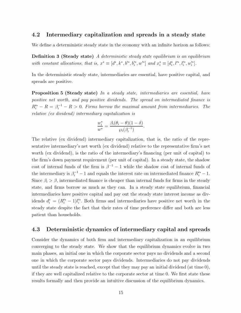
4.2 Intermediary capitalization and spreads in a steady state

We define a deterministic steady state in the economy with an infinite horizon as follows:

Definition 3 (Steady state) A deterministic steady state equilibrium is an equilibrium

with constant allocations, that is, x∗ ≡ [d∗, k∗, b′∗, b′∗i , w′∗] and x∗i ≡ [d∗

i , l′∗, l′∗i , w′∗

i ].

In the deterministic steady state, intermediaries are essential, have positive capital, and

spreads are positive.

Proposition 5 (Steady state) In a steady state, intermediaries are essential, have

positive net worth, and pay positive dividends. The spread on intermediated finance is

R′∗i − R = β−1

i − R > 0. Firms borrow the maximal amount from intermediaries. The

relative (ex dividend) intermediary capitalization is

w∗i

w∗ =βi(θi − θ)(1 − δ)

℘i(β−1i )

.

The relative (ex dividend) intermediary capitalization, that is, the ratio of the repre-

sentative intermediary’s net worth (ex dividend) relative to the representative firm’s net

worth (ex dividend), is the ratio of the intermediary’s financing (per unit of capital) to

the firm’s down payment requirement (per unit of capital). In a steady state, the shadow

cost of internal funds of the firm is β−1 − 1 while the shadow cost of internal funds of

the intermediary is β−1i − 1 and equals the interest rate on intermediated finance R′∗

i − 1.

Since βi > β, intermediated finance is cheaper than internal funds for firms in the steady

state, and firms borrow as much as they can. In a steady state equilibrium, financial

intermediaries have positive capital and pay out the steady state interest income as div-

idends d∗i = (R′∗

i − 1)l′∗i . Both firms and intermediaries have positive net worth in the

steady state despite the fact that their rates of time preference differ and both are less

patient than households.

4.3 Deterministic dynamics of intermediary capital and spreads

Consider the dynamics of both firm and intermediary capitalization in an equilibrium

converging to the steady state. We show that the equilibrium dynamics evolve in two

main phases, an initial one in which the corporate sector pays no dividends and a second

one in which the corporate sector pays dividends. Intermediaries do not pay dividends

until the steady state is reached, except that they may pay an initial dividend (at time 0),

if they are well capitalized relative to the corporate sector at time 0. We first state these

results formally and then provide an intuitive discussion of the equilibrium dynamics.

15

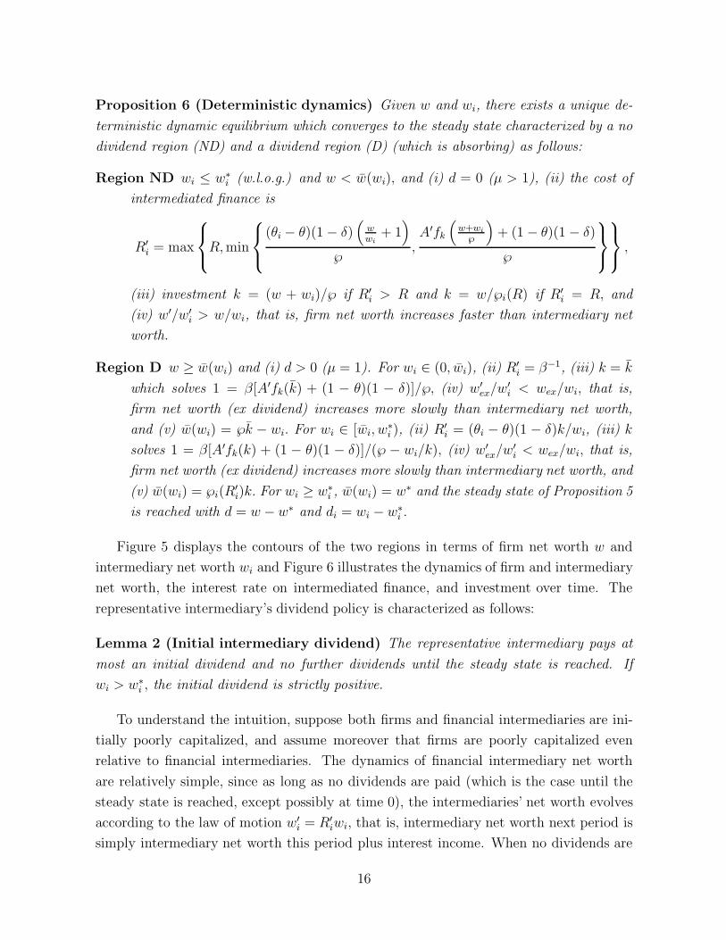
Proposition 6 (Deterministic dynamics) Given w and wi, there exists a unique de-

terministic dynamic equilibrium which converges to the steady state characterized by a no

dividend region (ND) and a dividend region (D) (which is absorbing) as follows:

Region ND wi ≤ w∗i (w.l.o.g.) and w < w(wi), and (i) d = 0 (µ > 1), (ii) the cost of

intermediated finance is

R′i = max

R,min

(θi − θ)(1 − δ)(

wwi

+ 1)

℘,A′fk

(w+wi

℘

)+ (1 − θ)(1 − δ)

℘

,

(iii) investment k = (w + wi)/℘ if R′i > R and k = w/℘i(R) if R′

i = R, and

(iv) w′/w′i > w/wi, that is, firm net worth increases faster than intermediary net

worth.

Region D w ≥ w(wi) and (i) d > 0 (µ = 1). For wi ∈ (0, wi), (ii) R′i = β−1, (iii) k = k

which solves 1 = β[A′fk(k) + (1 − θ)(1 − δ)]/℘, (iv) w′ex/w

′i < wex/wi, that is,

firm net worth (ex dividend) increases more slowly than intermediary net worth,

and (v) w(wi) = ℘k − wi. For wi ∈ [wi, w∗i ), (ii) R′

i = (θi − θ)(1 − δ)k/wi, (iii) k

solves 1 = β[A′fk(k) + (1 − θ)(1 − δ)]/(℘ − wi/k), (iv) w′ex/w

′i < wex/wi, that is,

firm net worth (ex dividend) increases more slowly than intermediary net worth, and

(v) w(wi) = ℘i(R′i)k. For wi ≥ w∗

i , w(wi) = w∗ and the steady state of Proposition 5

is reached with d = w − w∗ and di = wi − w∗i .

Figure 5 displays the contours of the two regions in terms of firm net worth w and

intermediary net worth wi and Figure 6 illustrates the dynamics of firm and intermediary

net worth, the interest rate on intermediated finance, and investment over time. The

representative intermediary’s dividend policy is characterized as follows:

Lemma 2 (Initial intermediary dividend) The representative intermediary pays at

most an initial dividend and no further dividends until the steady state is reached. If

wi > w∗i , the initial dividend is strictly positive.

To understand the intuition, suppose both firms and financial intermediaries are ini-

tially poorly capitalized, and assume moreover that firms are poorly capitalized even

relative to financial intermediaries. The dynamics of financial intermediary net worth

are relatively simple, since as long as no dividends are paid (which is the case until the

steady state is reached, except possibly at time 0), the intermediaries’ net worth evolves

according to the law of motion w′i = R′

iwi, that is, intermediary net worth next period is

simply intermediary net worth this period plus interest income. When no dividends are

16

paid, intermediaries lend out all their funds at the interest rate R′i. Of course, the interest

rate R′i needs to be determined in equilibrium.

Given our assumptions, the corporate sector’s net worth, investment and loan demand

evolve in several phases, which are reflected in the dynamics of the equilibrium interest

rate. If firms are initially poorly capitalized even relative to financial intermediaries,

as we assume, loan demand is low and intermediaries are relatively well capitalized. In

this case, except for a potential initial dividend, intermediaries conserve net worth to

meet future loan demand by lending some of their funds to households (see Panel B3 of

Figure 6) and spreads are zero, that is, R′i = R (see Panel B1). In fact, the intermediaries’

lending to households exceeds their lending to the corporate sector early on. Corporate

investment is then k = w/℘i(R). Intermediaries accumulate net worth at rate R in this

phase while the corporate sector accumulates net worth at a faster rate, given the high

marginal product; thus, the net worth of the corporate sector rises relative to the net

worth of intermediaries. In Figure 6, this phase last from time t = 0 to t = 3, except

that the intermediary pays an initial dividend at t = 0, since Figure 6 considers an initial

drop in corporate net worth only.

Eventually, the increased net worth of the corporate sector raises loan demand so

that intermediated finance becomes scarce. The corporate sector then borrows all the

funds intermediaries are able to lend and invests k = (w + wi)/℘. The interest rate on

intermediated finance is determined by the collateral constraint, which is binding, and

equals R′i = (θi − θ)(1 − δ) (w/wi + 1) /℘. Note that since corporate net worth increases

faster than intermediary net worth, the interest rate on intermediated finance rises in

this phase. As the corporate sector accumulates net worth, it can pledge more and the

equilibrium interest rate rises. In Figure 6, this occurs between t = 3 and t = 4.

As the net worth and investment of the corporate sector continues to rise faster than

intermediary net worth, the increase in firms’ collateral means that firms’ ability to pledge

no longer constrains their ability to raise intermediated finance. Intermediated finance is

scarce in this phase because of limited intermediary net worth, however, and so spreads are

high but declining. The law of motion of investment is as in the previous phase k = (w +

wi)/℘, while the equilibrium interest rate on intermediated finance is determined by R′i =

[A′fk(k) + (1 − θ)(1 − δ)]/℘. Both firm and intermediary net worth continue to increase,

and hence investment increases and the equilibrium interest rate on intermediated finance

decreases. In Figure 6, this occurs between t = 4 and t = 5.

Eventually, the interest rate on intermediated finance reaches β−1, the shadow cost of

internal funds of the corporate sector. At that point, corporate investment stays constant

and firms start to pay dividends. However, intermediaries continue to accumulate net

17

worth and the economy is not yet in steady state. As intermediaries accumulate net

worth, the corporate sector reduces its net worth by paying dividends. Essentially, the

corporate sector relevers as the supply of intermediated finance increases when financial

intermediary net worth increases. This is the case at t = 5 and t = 6 in Figure 6.

Once intermediary capital is sufficiently high to accommodate the entire loan demand

of the corporate sector at an interest rate β−1, the cost of intermediated funds decreases

further. As the interest rate on intermediated finance is now below the shadow cost of

internal funds of the corporate sector, the collateral constraint binds again. Investment

increases due to the reduced cost of intermediated financing. This phase lasts from t = 7

to t = 9 in Figure 6. Eventually, intermediaries accumulate their steady state level of net

worth and the cost of intermediated finance reaches β−1i , the intermediaries’ shadow cost

of internal funds. The steady state is reached at t = 9 in Figure 6.

We emphasize two key aspects of the dynamics of intermediary capital, beyond the

fact that intermediary and firm net worth affect the dynamics jointly. First, intermediary

capital accumulates more slowly than corporate net worth in our model. Second, the

interest rate on intermediated finance is low when intermediaries conserve net worth to

meet the higher loan demand later on when the corporate sector is temporarily relatively

poorly capitalized. And vice versa, the corporate sector accumulates additional net worth

and spreads remain higher (and investment lower than in the steady state) as the corpo-

rate sector “waits” for intermediary net worth to rise and eventually reduce spreads, at

which point firms relever. The second two observations of course are a reflection of the

relatively slow pace of intermediary capital accumulation.

4.4 Dynamics of a credit crunch

Suppose the economy experiences a credit crunch, which we model here as an unantic-

ipated one-time drop in intermediary net worth wi. We assume that the economy is

otherwise deterministic and is in steady state when the credit crunch hits. Figure 7 il-

lustrates the effects of such a credit crunch on interest rates, net worth, intermediary

lending, and investment. The effect of a credit crunch depends on its size. Intermediaries

can absorb a small enough credit crunch simply by cutting dividends. But a larger drop

in intermediary net worth results in a reduction in lending and an increase in the spread

on intermediated finance. Moreover, the higher cost of intermediated finance increases

the user cost of capital (20) (as the premium on internal finance is either unchanged or

increases) and so investment drops. Thus, a credit crunch has real effects in our model.

Remarkably, investment drops even if the corporate sector is still well capitalized (that

is, even if w′∗ > w). The reason is that the cost of capital increases even if the corporate

18

sector is well capitalized, as intermediaries’ capacity to extend relatively cheap financing

is reduced. In that case, the credit crunch results in a jump in the interest rate on inter-

mediated finance to R′i = β−1 > R′∗

i = β−1i and an immediate drop in investment (and

capital, which drops to k < k∗). The real effects in our model are moreover persistent,

even if the corporate sector remains well capitalized. Indeed, the recovery of the real

economy can be delayed. After a sufficiently large credit crunch, investment and capital

remain constant at the lower level, and spreads remain constant at the elevated level,

until the intermediary sector accumulates sufficient capital to meet the loan demand. At

that point, intermediary interest rates start to fall and investment begins to recover, until

the economy eventually recovers fully.

If the corporate sector is no longer well capitalized after the credit crunch, the spread

on intermediated finance rises further and investment drops even more. This is the case

in Figure 7 at time 0 (see Panel B1 and B4). Moreover, after an initial partial recovery,

the recovery stalls, potentially for a long time (from time 1 to time 23 in Figure 7), in the

sense that the interest rate on intermediated finance remains at R′i = β−1 and investment

remains constant below its steady state level (in fact, capital remains constant at k), until

the intermediaries accumulate sufficient capital. Then the recovery resumes.

If net worth of both the intermediaries and the corporate sector drop at the same time,

for example, because of a one-time depreciation shock to capital, then investment and

output fall more substantially. The dynamics of the recovery from such a downturn are

as described in Section 4.3. It is noteworthy, though, that the spreads on intermediated

finance may or may not go up in such a general downturn, and in fact may well go down

despite the scarcity of intermediary capital. The point is that the lower net worth of the

corporate sector reduces loan demand, possibly by more than the drop in intermediary net

worth reduces loanable funds. If corporate loan demand drops sufficiently, intermediaries

may pay a one time dividend when the downturn hits, and then cut dividends to zero

until the economy recovers.

4.5 Comovement of firm and intermediary capital

Do the marginal value of firm and intermediary net worth comove? We consider this

question in a stochastic economy which is deterministic from time 1 onward. Importantly,

this allows both firms and intermediaries to engage in risk management at time 0 and

hedge the net worth available to them in different states s′ ∈ S at time 1. We first show

that the representative firm optimally engages in incomplete risk management, that is,

the collateral constraint for direct finance against at least one state s′ ∈ S must bind. We

then provide sufficient conditions for the marginal value of net worth of the representative

19

firm and the representative intermediary to comove.

Proposition 7 (Comovement of the value of firm and intermediary capital) In

an economy that is deterministic from time 1 onward and has constant expected produc-

tivity, (i) the representative firm must be collateral constrained for direct finance against

at least one state at time 1; (ii) the marginal value of firm and intermediary net worth

comove, in fact µ(s′)/µ(s′+) = µi(s′)/µi(s

′+), ∀s′, s′+ ∈ S, if λi(s

′) = 0, ∀s′ ∈ S. (iii) Sup-

pose moreover that there are just two states, that is, S = {s′, s′}. If only one of the

collateral constraints for direct finance binds, λ(s′) > 0 = λ(s′), then the marginal values

must comove, µ(s′) > µ(s′) and µi(s′) ≥ µi(s

′).

Proposition 7 implies that the marginal values of firm and intermediary net worth comove,

for example, when the intermediary has very limited net worth and hence the collateral

constraints for intermediated finance are slack for all states. They also comove if the firm

hedges one of two possible states, as then the intermediary effectively must be hedging

that state, too. Thus, the marginal value of intermediary net worth may be high exactly

when the marginal value of firm net worth is high, too. The marginal values may however

move in opposite directions, for example, if a high realization of productivity raises firm

net worth substantially, which lowers the marginal product of capital and hence the

marginal value of firm net worth, while it may raise loan demand substantially and hence

raise the marginal value of intermediary net worth.

5 Conclusion

We develop a dynamic theory of financial intermediation and show that the capital of

both the financial intermediary and corporate sector affect real economic activity, such

as firm investment, financing, and the spread between intermediated and direct finance.

Financial intermediaries are modeled as collateralization specialists that are better able to

collateralize claims than households themselves. Financial intermediaries require capital

as their ability to borrow against their collateralized loans is limited by households’ ability

to collateralize the assets backing the loans themselves.

The spread on intermediated finance is high when both firms and intermediaries are

poorly capitalized, and in particular when intermediaries are moreover poorly capitalized

relative to firms. Intermediary capital in our model accumulates more slowly than the

capital of firms, and thus spreads on intermediated finance may initially rise as loan

demand increases more than loanable funds as the net worth of the corporate sector

increases relative to the net worth of financial intermediaries. A credit crunch, that is,

20

a drop in intermediary net worth results in a drop in intermediated finance, a rise in

spreads on intermediated loans, and a drop in real activity. The recovery can be delayed,

or stall, with real activity constant at a reduced level and persistently high spreads on

intermediated finance, because it takes time for intermediaries to reaccumulate sufficient

net worth. In the cross section, the model predicts that more constrained firms borrow

from financial intermediaries, consistent with stylized facts. In addition, the model shows

that the marginal value of intermediary and firm net worth may comove. Our model may

provide a useful framework for the analysis of the dynamic interaction between financial

structure and economic activity.

21

Appendix

Appendix A: Intermediated vs. direct finance in the cross section

This appendix considers the static environment without uncertainty of Section 3 taking

the spread on intermediated finance as given to show that our model has plausible im-

plications for the choice between intermediated and direct finance in the cross section

of firms. Consider the firm’s problem taking the interest rate on intermediated finance

R′i as given. Each firm maximizes (22) subject to (9) through (12) given its net worth

w. Severely constrained firms borrow as much as possible from intermediaries while less

constrained firms borrow less from intermediaries and dividend paying firms do not bor-

row from intermediaries at all, consistent with the cross sectional stylized facts. These

cross-sectional results are similar to the ones in Holmstrom and Tirole (1997).

Proposition 8 (Intermediated vs. direct finance across firms) Suppose R′i > β−1.13

(i) Firms with net worth w ≤ wl borrow as much as possible from intermediaries, firms

with net worth wl < w < wu borrow a positive amount from intermediaries but less than

the maximal amount, and firms with net worth exceeding wu do not borrow from interme-

diaries, where 0 < wl < wu. (ii) Only firms with net worth exceeding w pay dividends at

time 0, where wu < w < ∞. (iii) Investment is increasing in w and strictly increasing

for w ≤ wl and wu < w < w.

Intermediated finance is costlier than direct finance. Indeed, under the conditions of

the proposition, intermediated finance is costlier than the shadow cost of internal finance

of well capitalized firms. Thus, well capitalized firms, which pay dividends, do not borrow

from financial intermediaries. In contrast, firms with net worth below some threshold

(wu) have a shadow cost of internal finance which is sufficiently high that they choose to

borrow a positive amount from intermediaries. For severely constrained firms, with net

worth below wl, the shadow cost of internal funds is so high that they borrow as much as

they can from intermediaries, that is, their collateral constraint for intermediated finance

binds. Moreover, more constrained firms have lower investment and are hence smaller.

The cross-sectional capital structure implications are plausible: smaller (and more

constrained) firms borrow more from financial intermediaries and have higher costs of

financing, while larger (and less constrained firms) borrow from households, for example

in bond markets, and have lower financing costs.

13We consider the case in which R′i > β−1 since, proceeding analogously as in the first part of the

proof, one can show that R′i < β−1 would imply that λ′

i > 0 and thus the cross sectional financingimplications would be trivial as all firms would borrow the maximal amount from intermediaries. WhenR′

i = β−1, this would also be true without loss of generality.

22

Appendix B: Proofs

Proof of Proposition 1. Using (16) and the fact that ν′i = 0 (proved below in Lemma 1,

part (iii)), we have (R′i)−1 = βµ′/µ + βλ′

i/µ and, taking expectations,

1

R + ρi≡ E

[(R′

i)−1

]=

1

R + ρ+ E

[β

λ′i

µ

]

and hence ρ ≥ ρi with equality iff E[λ′i] = 0. Moreover, since R′

i ≥ R (proved below

in Lemma 1, part (i)), ρi ≥ 0. Finally, using (15), we have 1/(R + ρ) ≡ E[βµ′/µ] =

1/R − E[βλ′/µ], implying that ρ > 0 iff E[λ′] > 0. 2

Proof of Proposition 2. First, consider the intermediary’s problem. The first order

conditions are (4)-(6) and µ′i = 1 + η′

d, where βiη′d is the multiplier on the constraint

w′i ≥ 0. Since (3) holds with equality, the non-negativity constraints on l′ and l′i render

the non-negativity constraint on w′i redundant and hence µ′

i = 1. Using (5) we have

η′ = (Rβi)−1µi − 1 ≥ (Rβi)

−1 − 1 > 0 (and l′ = 0) and similarly using (6) η′i > 0 as long

as R′i < β−1

i . Therefore, for l′i > 0 it is necessary that R′i ≥ β−1

i . If R′i > β−1

i , then µ′i > 1

(and l′i = wi) while if R′i = β−1

i , 0 ≤ l′i ≤ wi.

Now consider the representative firm’s problem. The first order conditions are (4)-(6)

and µ′ = 1 + ν′d, where βν ′

d is the multiplier on the constraint w′ ≥ 0. Proceeding as in

the proof of Proposition 8 one can show that µ′ = 1. Suppose ν′i > 0 (and hence b′i = 0).

Since k > 0, (12) is slack and λ′i = 0. Using (13) and (16) we have 1 ≤ µ < R′

iβ which

implies that R′i > β−1. But at such an interest rate on intermediated finance l′i = wi > 0,

which is not an equilibrium as b′i = 0. Therefore, ν′i = 0 and R′

i ≤ β−1. Moreover, if

R′i < β−1, then λ′

i = (R′iβ)−1µ − 1 > 0 and hence b′i = (R′

i)−1(θi − θ)k(1 − δ) > 0. Since

l′i = 0 if R′i < β−1

i , we have R′i ∈ [β−1

i , β−1] in equilibrium. The firm’s investment Euler

equation (19) simplifies to 1 = β(1/µ)[A′fk(k)+(1−θi)(1−δ)]/℘i(R′i). Given the interest

rate on intermediated finance, the firm’s problem induces a concave value function and

thus µ (weakly) decreases in w, implying that k (weakly) increases.

We first show that intermediaries are well capitalized and there is a minimum spread

on intermediated finance β−1i − R > 0 for all levels of firm net worth when wi ≥ w∗

i and

for levels of firm net worth w ≤ w(wi) when wi < w∗i . If R′

i = β−1i , a well capitalized firm

invests k∗ which solves (19) specialized to 1 = β[A′fk(k∗)+(1− θi)(1− δ)]/℘i(β

−1i ), while

less well capitalized firms invests k ≤ k∗. The intermediary can meet the required demand

for intermediated finance for any level of firm net worth w if wi ≥ w∗i ≡ βi(θi−θ)k∗(1−δ).

Suppose instead that wi < w∗i . In this case the intermediary is able to meet the firm’s loan

demand at R′i = β−1

i only if the firm is sufficiently constrained; the constrained firm invests

23

k = w/℘i(β−1i ) using (9), (11), and (12) at equality, and thus b′i = βi(θi − θ)k(1− δ); the

intermediary can meet this demand as long as w ≤ w(wi) ≡ ℘i(β−1i )/[βi(θi − θ)(1− δ)]wi.

Suppose now that wi < w∗i and w > w(wi) as defined above. First, consider wi ∈

[wi, w∗i ) where wi ≡ β(θi − θ)k(1 − δ) and 1 = β[A′fk(k) + (1 − θ)(1 − δ)]/℘, that is, wi

is the loan demand of the well capitalized firm when the cost of intermediated finance

is R′i = β−1. Note that R′

i < β−1 on (wi, w∗i ) since the intermediary has more than

enough net worth to accommodate the loan demand of the well capitalized firm (and

thus any constrained firm) at R′i = β−1. Thus, the firm’s collateral constraint binds,

that is, wi = (R′i)−1(θi − θ)k(1 − δ). If the firm is poorly capitalized, d = 0 and (9)

implies w + wi = ℘k, and R′i = (θi − θ)(1 − δ)(w/wi + 1). If the firm is well capitalized,

µ = 1 and k(wi) solves 1 = β[A′fk(k(wi)) + (1 − θi)(1 − δ)]/[℘ − wi/k(wi)]. Moreover,

w(wi) ≡ ℘k(wi) − wi and for w ≥ w(wi) the cost of intermediated finance is constant

at R′i(wi) = (θi − θ)k(wi)(1 − δ)/wi. Note that R′

i(w∗i ) = β−1

i and w(w∗i ) = ℘k∗ − w∗

i =

℘i(β−1i )k∗ = w(w∗

i ), that is, the two boundaries coincide at w∗i . In contrast, at wi we

have w(wi) = ℘i(β−1i )/[βi(θi − θ)(1 − δ)]wi = ℘i(β

−1i )β/βik = ℘kβ/βi − wi < w(wi) and

R′i(wi) = β−1.

Finally, consider wi ∈ (0, wi) and w > w(wi) as defined above. If the firm is well

capitalized (16) implies λ′i = (R′

iβ)−1 − 1 ≥ 0. Moreover, since wi < wi the intermediary

cannot meet the well capitalized firm’s loan demand at R′i = β−1 and thus the cost

of intermediated finance is in fact β−1 and λ′i = 0, that is, the collateral constraint

for intermediated finance does not bind. Thus, the firm’s investment Euler equation (19)

simplifies to 1 = β[A′fk(k)+(1−θi)(1−δ)]/℘i(β−1) which is solved by k as defined earlier

in the proof. Define w(wi) ≡ ℘k−wi; the firm is well capitalized for w ≥ w(wi). Suppose

w < w(wi) and hence µ > 1. If the collateral constraint for intermediated finance does not

bind, then (16) implies R′i = β−1µ > β−1 and (19) implies R′

i = [A′fk(k)+(1−θ)(1−δ)]/℘,

while (9) yields w + wi = ℘k. Observe that k < k and R′i decreases in w. If instead

the collateral constraint binds, then R′i = (θi − θ)k(1 − δ)/wi and w + wi = ℘k (so

long as w > w(wi)). Note that k and R′i increase in w in this range. The collateral

constrain is just binding at w(wi) ≡ ℘k(wi)−wi where [A′fk(k(wi))+(1− θ)(1− δ)]/℘ =

(θi − θ)k(wi)(1 − δ)/wi.

We now show that if the collateral constraint for intermediated finance binds at some

w < w(wi) then it binds for all w− < w. Note that d = 0 in this range and w + wi = ℘k.

At w−, either b′−i < wi and R′i = β−1

i and hence λ′−i = (β−1

i β)−1µ− − 1 > 0 or b′−i = wi

and w−+wi = ℘k−, implying k− < k. Suppose the collateral constraint for intermediated

finance is slack at w−. Then R′−i b′−i < (θi − θ)k−(1 − δ) < (θi − θ)k(1 − δ) = R′

ib′i and

24

since b′−i = wi and b′i ≤ wi by above R′−i wi < R′

ib′i ≤ R′

iwi which implies R′−i < R′

i. But

R′−i β = µ− = β

A′fk(k−) + (1 − θi)(1 − δ)

℘ − (R′−i )−1(θi − θ)(1 − δ)

> βA′fk(k) + (1 − θi)(1 − δ)

℘ − (R′i)−1(θi − θ)(1 − δ)

= µ > R′iβ

or R′−i > R′

i, a contradiction.

Moreover, w(wi) < w(wi) < w(wi) on wi ∈ (0, wi). Suppose, by contradiction,

that w(wi) ≤ w(wi) and recall that w(wi) + wi = ℘k and w(wi) + wi = ℘k(wi),

so k(wi) ≤ k. But R′i(wi) = (θi − θ)k(wi)(1 − δ)/wi ≤ (θi − θ)k(1 − δ)/wi = β−1

i .

But if R′i(wi) ≤ β−1

i , then at w(wi) we have µ = R′i(wi)β < 1 (since the collat-

eral constraint is slack), a contradiction. Thus, w(wi) < w(wi). Suppose, again by

contradiction, that w(wi) ≤ w(wi) and hence k ≤ k(wi). Recall that k(wi) solves

[A′fk(k(wi)) + (1 − θ)(1 − δ)]/℘ = (θi − θ)k(wi)(1 − δ)/wi. At wi this equation is solved

by k (and R′i(wi) = β−1), but since wi < wi, k(wi) < k, a contradiction. Moreover, as

wi → 0, k(wi) → 0 and w(wi) = ℘k(wi) − wi → 0. 2

Proof of Proposition 3. Consider a deterministic economy. Suppose intermediaries

pay out their entire net worth at some point. From that point on, the firm’s problem is

as if there is no intermediary. We first characterize the solution to this problem and then

show that the solution implies shadow interest rates on intermediated finance at which it

would not be optimal for intermediaries to exit.

To characterize the solution in the absence of intermediaries, consider a steady state

at which µ = µ′ ≡ µ and note that (15) implies λ′ = ((Rβ)−1 − 1)µ > 0. The investment

Euler equation (19) simplifies to 1 = β[A′fk(k) + (1 − θ)(1 − δ)/℘ which defines k. The

firm’s steady state net worth is w′ = A′f(k) + (1 − θ)k(1 − δ) and the firm pays out

d = w′ − ℘k = A′f(k) − k[1 − (R−1θ + (1 − θ))(1 − δ)]

> A′f(k) − β−1k[1 − (R−1θ + β(1 − θ))(1 − δ)]

=

∫ k

0

[A′fk(k) − β−1(1 − (R−1θ + β(1− θ))(1 − δ))]dk > 0.

Therefore, µ = 1. Investment k is feasible as long as w ≥ w = w′ − d. Whenever w < w,

k < k and hence using (19) we have µ/µ′ = β[A′fk(k) + (1 − θ)(1 − δ)]/℘ > 1. The

shadow interest rate on intermediated finance is R′i = β−1µ/µ′ ≥ β−1 for all values of

w. But then it cannot be optimal for intermediaries to pay out all their net worth in

a deterministic economy as keeping ε > 0 net worth for one more period improves the

objective by (βiR′i − 1)ε > 0.

Consider now an eventually deterministic economy. From time T onward, the economy

is deterministic and the conclusion obtains by above as long as the intermediary has

25

positive net worth in all states at time T . Suppose not, that is, suppose intermediary net

worth is zero for some state. As before the discounted marginal value on an infinitesimal

amount of intermediary net worth at time T lent out for one period is at least βiR′i ≥

βiβ−1 > 1 since R′

i ≥ β−1. Lending for τ periods thus guarantees a discounted marginal

value of (βiβ)τ . As τ → ∞, the marginal value grows without bound. (Note that since

we consider an infinitesimal amount, the collateral constraint cannot be biding for any

finite τ .) The expected marginal value of this lending policy at time 0 is at least (βiR)T

times the marginal value at time T and hence grows without bound as τ → ∞.

But the marginal value of intermediary net worth at time 0 is finite as either the inter-

mediary pays dividends and the marginal value is one, or the intermediary saves into at

least one state at R′i and thus µi = R′

iβµ′i and R′

i is bounded above by (12) and otherwise

R′i = R. Furthermore, µ′

i is bounded by a similar argument going forward until dividends

are paid at which point the marginal value is one. But then it cannot be an equilibrium

for intermediaries to pay out all their net worth. 2

Proof of Lemma 1. Part (i): If R′i < R, then using (15) and (16) we have 0 <

(R−R′i)βµ′ ≤ R′

iβλ′i and thus b′i > 0. But (5) and (6) imply that 0 < (R−R′

i)βµ′i ≤ R′

iβη′i

and thus l′i = 0, which is not an equilibrium.

Part (ii): Given ν′i = 0 (see part (iii)), (15) and (16) imply that λ′ = (R′

i/R − 1)µ′ +

R′i/Rλ′

i ≥ λ′i.

Part (iii): First, suppose to the contrary that ν′i > 0. Then λ′

i = 0 as b′i = 0 <

(R′i)

−1(θi − θ)k(1 − δ) implies that (12) is slack. Using (16) and (15) we have βµ′R′i >

µ ≥ βµ′R and thus R′i > R. Equations (5) and (6) imply that Rη′−R′

iη′i = (R′

i−R)µ′i > 0

and thus η′ > 0 and l′ = 0. But if w′i > 0, which is always true under the conditions of

Proposition 3, we have l′i = (R′i)−1w′

i > 0 = b′i, which is not an equilibrium. If instead

w′i = 0, then l′i = 0 and we can set R′

i = (βµ′/µ)−1 and η′i = 0 w.l.o.g.

Part (iv): Suppose to the contrary that η′i > 0 (and hence l′i = 0). Since intermediaries

never pay out all their net worth in a deterministic economy, equation (3) implies 0 <

w′i ≤ Rl′ and hence η′ = 0. But then (5) and (6) imply βiµ

′i/µiR = 1 > βiµ

′i/µiR

′i or

R > R′i contradicting the result of part (i). Thus, η′

i = 0 and µ′i = (βiR

′i)

−1µi.

Part (v): Suppose λ′ = 0. Then (15) reduces to 1 = βµ′/µR and thus 1 ≤ µ = βRµ′ <

µ′ and d′ = 0. By part (ii), λ′i = 0 and using (16) we have R′

i = R, µ′i = (βR)−1µi >

1, and d′i = 0. The investment k∗∗ solves R = [A′fk(k

∗∗) + (1 − θi)(1 − δ)]/℘i(R) or

R − 1 + δ = A′fk(k∗∗); this is the first best investment when dividends are discounted at

R and it can never be optimal to invest more than that. To see this use (19) and note

[A′fk(k) + (1 − θi)(1 − δ)]/℘i(R′i) = µ/(βµ′) ≥ R = [A′fk(k

∗∗) + (1 − θi)(1 − δ)]/℘i(R),

26

that is, fk(k) ≥ fk(k∗∗). Note that the firm’s net worth next period, using (10) and (19),

is

w′ = A′f(k∗∗) + (1 − θi)(1 − δ)k∗∗ − [Rb′ − θ(1 − δ)k∗∗]− [Rb′i − (θi − θ)(1 − δ)k∗∗]

> R℘i(R)k∗∗ − [Rb′ − θ(1 − δ)k∗∗] − [Rb′i − (θi − θ)(1 − δ)k∗∗] = R[k∗∗ − b′ − b′i]

= Rwex.

Note that d′ = 0, d′i = 0, k′ ≤ k∗∗, and w′ > wex, and from (9) next period, k′ = w′+b′′+b′′i .

If R′′i > R, then b′′i = w′

i and b′′ = R−1θ(1 − δ)k′. Therefore, ℘k′ = w′ + w′i, but using

(9) we have ℘k∗∗ ≤ k∗∗ − b′ = wex + b′i < w′ + w′i = ℘k′, a contradiction. If R′′

i = R,

then b′′ + b′′i = k′ − w′ < k∗∗ − wex = b′ + b′i, that is, the firm is paying down debt, and

w′′ > w′ and w′′i > w′

i. But then w and wi grow without bound unless the firm or the

intermediary eventually pay a dividend. But since µ and µi are strictly increasing as long

as R′i = R, if either pays a dividend at some future date, then µ < 1 or µi < 1 currently,

a contradiction. 2

Proof of Proposition 5. First, note that k∗ > 0 due to the Inada condition and hence

w′∗ ≥ A′f(k∗) + k∗(1 − θi)(1 − δ) > 0. Moreover, d∗ > 0 since otherwise the value would

be zero which would be dominated by paying out all net worth. Hence, µ∗ = µ′∗ = 1. By

Proposition 3 intermediary net worth is positive and hence d∗i > 0 (arguing as above),

which implies µ∗i = µ′∗

i = 1. But then η′∗ = (Rβi)−1 − 1 > 0 and l′∗i > 0 (and η′∗

i = 0),

since otherwise intermediary net worth would be 0 next period. Therefore, R′∗i = β−1

i ,

and thus λ′∗i = (β−1

i β)−1 − 1 > 0, that is, the firm’s collateral constraint for interme-

diated finance binds. Moreover, k∗ solves 1 = β[A′fk(k∗) + (1 − θi)(1 − δ)]/℘i(β

−1i )

and d′∗, b′∗, b′∗i , and w′∗ are determined by (9)-(12) at equality. Specifically, d∗ =

A′f(k∗)+k∗(1−θi)(1−δ)−℘i(β−1i )k∗ > 0 and b′∗i = βi(θi−θ)k∗(1−δ). The net worth of

the firm after dividends is w∗ = ℘i(β−1i )k∗. Finally, l′∗i = b′∗i = w∗

i and d∗i = (β−1

i −1)w∗i . 2

Proof of Proposition 6. Consider first region D and take w ≥ w(wi) (to be defined

below) and d > 0 forever (µ = µ′ = 1). The investment Euler equation then implies

1 = β[A′fk(k) + (1 − θi)(1 − δ)]/℘i(Ri). If the collateral constraint for intermediated

finance (12) does not bind, then µ = R′iβµ′, that is, R′

i = β−1, and investment is constant

at k which solves 1 = β[A′fk(k)+(1−θi)(1−δ)]/℘i(β−1) or, equivalently, 1 = β[A′fk(k)+

(1 − θ)(1− δ)]/℘. Define w(wi) ≡ ℘k −wi and wi = β(θi − θ)k(1− δ). At wi, (12) is just

binding. For wi ∈ (0, wi), (12) is slack. Moreover, w′i = β−1wi and, if w′

i ∈ (0, wi), the

ex dividend net worth is wex = w(wi) both in the current and next period, and we have

27

immediately w′ex/w

′i < wex/wi. Further, using (10) and (19) we have

w′ = A′f(k) + (1 − θ)k(1 − δ)− R′iwi > [A′fk(k) + (1 − θ)(1 − δ)]k − R′

iwi = R′iw(wi).

But w′ex = w(w′

i) < w(wi)w′i/wi = R′

iwex, so d′ = w′ − w′ex > 0. For wi ∈ [wi, w

∗i ),

(12) binds and k(wi) solves 1 = β[A′fk(k(wi)) + (1 − θi)(1 − δ)]/[℘ − wi/k(wi)] and

R′i = (θi − θ)k(wi)/wi(1 − δ). Note that the last two equations imply that k(wi) ≥ k,

wi/k(wi) ≥ wi/k, and R′i ≤ β−1 in this region. As before, define w(wi) = ℘k(wi) − wi

and note that the ex dividend net worth is wex = w(wi). Suppose w+i > wi then k(w+

i ) >

k(wi), k(w+i )/w+

i < k(wi)/wi, and w+ex/w

+i = ℘k(w+

i )/w+i − 1 < wex/wi. Moreover,

w′i = R′

iwi > wi and hence k (strictly) increases and R′i (strictly) decreases in this region.

Proceeding as before,

w′ = A′f(k(wi)) + (1 − θi)k(wi)(1 − δ) > [A′fk(k(wi)) + (1 − θi)(1 − δ)]k(wi)

≥ R′iβ[A′fk(k(wi)) + (1 − θi)(1 − δ)]k(wi) = R′

iw(wi).

But w′ex = w(w′

i) < w(wi)w′i/wi = R′

iwex, so d′ = w′ − w′ex > 0. Finally, if wi ≥ w∗

i and

w ≥ w(wi) = w∗, the steady state of Proposition 5 is reached.

We now show that the above policies are optimal for both the firm and the interme-

diary given the interest rate process in region D and hence constitute an equilibrium.

Since R′i > β−1

i before the steady state is reached, the intermediary lends its entire net

worth to the firm, l′i = wi, and does not pay dividends until the steady state is reached.

Hence, the intermediary’s policy is optimal. To see that the firm’s policy is optimal in

region D, suppose that the firm follows the optimal policy from the next period onward

but sets d = 0 in the current period. If the firm invests the additional amount, then

k = (wi + w)/℘ > k and w′ > w′ (and therefore µ′ = 1). The investment Euler equation

requires 1 = β/µ[A′fk(k)+ (1− θi)(1− δ)]/℘i(R′i), but since fk(k) < fk(k) and k satisfies

the investment Euler equation at µ = µ′ = 1, this implies µ < 1, a contradiction. Suppose

the firm instead invests the same amount k = k but borrows less b′i < b′i. Then w′ > w′,

µ′ = 1, and from (19) µ = 1. If R′i < β−1, then (12) is binding, a contradiction. If

R′i = β−1, then the firm is indifferent between paying dividends in the current period or

in the next period. But in equilibrium b′i = wi and hence d = d > 0 for the representative

firm. By induction starting at the steady state and working backwards, the firm’s policy

is optimal in region D. Further, we show in Lemmata 3 and 4 that the equilibrium in

region D is the unique equilibrium converging to the steady state.

Consider now region ND with wi ≤ w∗i (as Lemma 2 shows) and w < w(wi) as defined

in the characterization of region D above and d = 0. Denote the firm’s ex dividend

net worth by wex ≤ w. There are 3 cases to consider: wex/wi > w/wi, wex/wi ∈[w∗/w∗

i , w/wi], and wex/wi < w∗/w∗i .

28

First, if wex/wi > w/wi, then wex +wi < w(wi)+wi = w+ wi and k ≤ (wex +wi)/℘ <

(w + wi)/℘ = k. Note that since b′i ≤ wi − di ≤ wi, we have wex/b′i ≥ wex/wi > w/wi. If

(12) binds, then R′i = (θi−θ)(1−δ)(wex/b

′i +1)/℘ > (θi−θ)(1−δ)(w/wi +1)/℘ = β−1. If

(12) does not bind, then R′i = [A′fk(k)+(1−θ)(1−δ)]/℘ > [A′fk(k)+(1−θ)(1−δ)]/℘ =

β−1. In either case, R′i > β−1, and hence d = 0, di = 0, and b′i = wi.

Second, consider wex/wi ∈ [w∗/w∗i , w/wi]. If wex/b

′i > w/wi we are in the first region

and hence di = 0 and b′i = wi, a contradiction. Hence, w.l.o.g. wex/b′i ∈ [w∗/w∗

i , w/wi].

Take wi such that wex/b′i = w(wi)/wi. Note that (12) binds at wi and w(wi), and thus

b′i + wex < wi + w(wi) and moreover k < k(wi). If (12) does not bind, then

R′i(wi) = (θi − θ)(1 − δ)(w(wi)/wi + 1)/℘ > (θi − θ)(1 − δ)(wex/b

′i + 1)/℘ > R′

i

= [A′fk(k) + (1 − θ)(1 − δ)]/℘ > [A′fk(k(w)) + (1 − θ)(1 − δ)]/℘.

But since (12) binds at wi and w(wi), R′i(wi) < [A′fk(k(w)) + (1 − θ)(1 − δ)]/℘, a

contradiction. Therefore, (12) binds and R′i = R′

i(wi). From (19), βµ′/µ[A′fk(k) + (1 −θi)(1− δ)]/℘i(R

′i) = 1 = β[A′fk(k(wi))+ (1− θi)(1− δ)]/℘i(R

′i(wi)) and, since k < k(wi),

µ > µ′ ≥ 1, that is, d = 0. Further, if wex/wi ∈ (w∗/w∗i , w/wi], then R′

i ∈ (β−1i , β−1], and

thus di = 0 and b′i = wi. If wex/wi = w∗/w∗i , then either di > 0 or b′i < wi yields R′

i > β−1i

and therefore di = 0 and b′i = wi at such wex and wi as well.

Third, consider wex/wi < w∗/w∗i . As before, w.l.o.g. wex/b

′i < w∗/w∗

i . Then from (12),

R′i ≤ (θi−θ)(1−δ)(wex/b

′i +1)/℘ < (θi−θ)(1−δ)(w∗/w∗

i +1)/℘ = β−1i , that is, R′

i < β−1i .

From (19), βµ′/µ[A′fk(k)+(1−θi)(1−δ)]/℘i(R′i) = 1 = β[A′fk(k

∗)+(1−θi)(1−δ)]/℘i(β−1i )

and, since k < k∗ and R′i < β−1

i , µ > µ′ ≥ 1, that is, d = 0. Moreover, (12) binds, since

otherwise β−1i > R′

i = [A′fk(k) + (1 − θ)(1 − δ)]/℘ > [A′fk(k∗) + (1 − θ)(1 − δ)]/℘, but

since in the steady state (12) binds β−1i < [A′fk(k

∗) + (1 − θ)(1 − δ)]/℘, a contradiction.

Thus, we conclude that d = 0, (property (i) in the statement of the proposition),

di = 0 (except possibly in the first period (see Lemma 2), that R′i satisfies the equation

in property (ii) of the proposition), and that b′i = wi and k = (w + wi)/℘ if R′i > R and

k = w/℘i(R) if R′i = R (property (iii)). Moreover, using (10) and (19) we have

w′ = A′f(k) + (1 − θi)(1 − δ)k − [R′ib

′i − (θi − θ)(1 − δ)k]

> R′i℘i(R

′i)k − [R′

ib′i − (θi − θ)(1 − δ)k] ≥ R′

i℘k − R′ib

′i = R′

iw,

which, together with the fact that w′i = R′

iwi, implies that w′/w′i > w/wi (property (iv)).

Note that the equilibrium is thus unique in region ND as well. 2

Proof of Lemma 2. We first show that di > 0 when wi > w∗i . If w ≥ w∗, the stationary

state is reached and the result is immediate. Suppose hence that w < w∗. Suppose

29

instead that di = 0. We claim that R′i < β−1

i for such wi and w. Either R′i = R and hence

the claim is obviously true or R′i > R, but then b′i = wi. Using (12) and (9) we have

R′i ≤ (θi−θ)(1−δ)k/b′i ≤ (θi−θ)(1−δ)(w/wi+1) < (θi−θ)(1−δ)(w∗/w∗

i +1) = β−1i , that

is, R ≤ R′i < β−1

i . But as long as di = 0, w′i = R′

iwi ≥ Rwi > wi, that is, intermediary

net worth keeps rising. If eventually firm net worth exceeds w∗, then the steady state is

reached and µ′i = 1 from then onward. But then µi = βiR

′iµ

′i = βiR

′i < 1, which is not

possible. The intermediary must pay a dividend in the first period, because if it pays a

dividend at any pont after that, an analogous argument would again imply that µi < 1 in

the first period, which is not possible. Similarly, if w < w∗ forever, then w > w∗i forever

and the firm must eventually pay a dividend in this region, as never paying a dividend

cannot be optimal. But by the same argument again then the dividend must be paid in

the first period.

To see that at most an initial dividend is paid and no further dividends are paid until

the steady state is reached, note that in equilibrium once R′i > β−1

i , then this is the case

until the steady state is reached. But as long as R′i > β−1

i , the intermediary does not pay

a dividend (and this is true w.l.o.g. also at a point where R′i = β−1

i before the steady state

is reached). Before this region is reached, R′i < β−1

i , but then the intermediary would not

postpone a dividend in this region, as other wise again µi = βiR′iµ

′i = βiR

′i < 1, which is

not possible. 2

Lemma 3 Consider an equilibrium with R′i ∈ [β−1

i , β−1] and µ = µ′ = 1 and assume the

equilibrium is unique from the next period onward. Consider another equilibrium interest

rate R′i, then k ≶ k and R′

i ≶ R′i is impossible.

Proof of Lemma 3. Using (19) at the two different equilibria, if k ≶ k and R′i ≶ R′

i,

then

µ

µ′ = βA′fk(k) + (1 − θi)(1 − δ)

℘i(R′i)

≷ βA′fk(k) + (1 − θi)(1 − δ)

℘i(R′i)

= 1 (23)

If k < k and R′i < R′

i = β−1i , then by (23) µ > µ′. Thus, µ > µ′R′

iβi implying that (12)

must be binding. But then the firm must pay a dividend and 1 = µ > µ′, a contradiction.

If k > k and R′i > R′

i and the collateral constraint binds at the original equilibrium,

then w′ ≥ A′f(k) + (1 − θ)i)(1 − δ)k > A′f(k) + (1 − θi)(1 − δ)k = w′. Since w′ > w′,

µ′ = 1, and the equilibrium is unique , µ′ = 1. By (23), µ < µ′ = 1, a contradiction.

If k > k and R′i > R′

i and the collateral constraint does not bind at the original

equilibrium, the R′i = β−1 (using (16)). But then µ/µ′ ≥ R′

iβ > 1 while (23) implies

µ/µ′ < 1, a contradiction. 2

30

Lemma 4 The equilibrium in region D is the unique equilibrium converging to the steady

state.

Proof of Lemma 4. The proof is by induction. First, note that if w ≥ w∗ and

wi ≥ w∗i , then the unique steady state is reached. Consider an equilibrium interest rate

R′i in region D and suppose the equilibrium is unique from the next period on. Suppose

R′i ∈ [β−1

i , β−1) and consider another equilibrium with R′i. If the collateral constraint

(12) binds at this equilibrium, then R′i = (θi − θ)(1− δ)k/wi ≷ (θi − θ)(1− δ)k/wi = R′

i,

which is impossible by Lemma (3). If the collateral constraint (12) does not bind at this

equilibrium and k < k, then R′i < (θi − θ)(1 − δ)k/wi < (θi − θ)(1 − δ)k/wi = R′

i, which

is also impossible by Lemma (3). If the collateral constraint (12) does not bind at this

equilibrium and k > k, by Lemma (3) R′i < Ri. But then by (16) µ/µ′ = βR′

i < βR′i < 1.

Since k > k and the collateral constraint binds at R′i, w′ > w′ implying µ′ = 1 and

by above inequality µ < 1, a contradiction. Thus for R′i ∈ [β−1

i , β−1) the equilibrium is

unique. Suppose R′i = β−1. By Lemma (3), we need only consider the two cases k ≷ k and

R′i ≶ R′

i = β−1. If k < k and R′i > β−1, (16) implies that µ > 1 and hence the firm does

not pay a dividend. But then the firm must be borrowing less from intermediaries, which

cannot be an equilibrium as l′i = wi at this interest rate. If k > k and R′i < R′

i = β−1, and

if (12) binds at R′i, R′

i = (θi − θ)(1− δ)k/wi > (θi − θ)(1 − δ)k/wi ≥ R′i, a contradiction;

if (12) instead does not bind at R′i, µ/µ′ = βR′

i < 1. Since k > k and R′ib

′i ≤ R′

iwi,

w′ > w′ implying µ′ = 1 and by above inequality µ < 1, a contradiction. Therefore the

equilibrium in region D is unique. 2

Proof of Proposition 7. Part (i): By assumption the expected productivity in the

first period equals the deterministic productivity from time 1 onward (denoted A′ here),

that is, E[A′] = A′. Define the first best level of capital kfb by r + δ = A′fk(kfb).

Using the definition of the user cost of capital the investment Euler equation (19) for the

deterministic case can be written as

r + δ +ρ

R + ρ(1 − θi)(1 − δ) +

ρi

R + ρi(θi − θ)(1 − δ) = RβA′fk(k

∗) < A′fk(k∗)

and thus k∗ < kfb. Now suppose that λ(s′) = 0, ∀s′ ∈ S. Part (ii) of Lemma 1 then

implies that λi(s′) = 0, ∀s′ ∈ S, and (15) and (16) simplify to µ = Rβµ′ and µ = R′

iβµ′,

implying that R′i = R, ∀s′ ∈ S, and that d′ = 0, ∀s′ ∈ S, as otherwise µ < 1. Moreover,

(6) simplifies to µi = Rβiµ′i and thus d′

i = 0, ∀s′ ∈ S, as well since otherwise µi < 1.

Investment Euler equation (19) reduces to r + δ = A′fk(kfb), that is, investment must be

kfb. We now show that this implies that the sum of the net worth of the intermediary

and the firm exceeds their steady state (cum dividend) net worth in at least one state,

31

which in turn implies that at least one of them pays a dividend, a contradiction. To see

this note that w′ = A′f(kfb) + kfb(1 − δ)− Rb′ − R′ib

′i and w′

i = Rl′ + R′il′i ≥ R′

il′i = R′

ib′i

and thus

w′+w′i ≥ A′f(kfb)+kfb(1−δ)−Rb′ ≥ A′f(kfb)+(1−θ)kfb(1−δ) > A′f(k∗)+(1−θ)k∗(1−δ)

whereas w′∗ + w′∗i = A′f(k∗) + (1 − θ)k∗(1 − δ). For A′ > A′, w′ + w′

i > w′∗ + w′∗i , and

either the intermediary or the firm (or both) must pay a dividend, a contradiction.

Part (ii): If λi(s′) = 0, ∀s′ ∈ S, then (βµ′/µ)−1 = R′

i = (βiµ′i/µi)

−1 where the first

equality uses (16) and the second equality uses (6) and the fact that part (iv) of Lemma 1

holds for an eventually deterministic economy.

Part (iii): Since λ(s′) = 0, λi(s′) = 0 by part (ii) of Lemma 1 and Ri(s

′) = R.

From (15), µ(s′) = µ(s′) + λ(s′) > µ(s′). Using (6), (βiµi(s′)/µi)

−1 = R ≤ Ri(s′) =

(βiµi(s′)/µi)

−1 and thus µi(s′) ≥ µi(s

′). 2

Proof of Proposition 8. The first order conditions are (13)-(16) and µ′ = 1+ ν′d where

βν ′d is the multiplier on the constraint w′ ≥ 0. By the Inada condition, (14) implies that

k > 0 and using (10) at equality and (11) and (12) we have d′ ≥ A′f(k)+k(1−θi)(1−δ) > 0

and µ′ = 1. But (13) and (15) imply 1 ≤ µ = Rβ + Rβλ′ and thus λ′ > 0 since Rβ < 1

by assumption; that is, all firms raise as much financing as possible from households.

Suppose the firm pays dividends at time 0. Then µ = µ′ = 1 and (16) implies

0 > 1−R′iβ = R′

iβλ′i −R′

iβν ′i and thus ν′

i = 1− (R′iβ)−1 > 0, b′i = 0, and λ′

i = 0; thus, the

firm does not use intermediated finance. Note that the problem of maximizing (22) subject

to (9) through (12) has a (weakly) concave objective and a convex constraint set and hence

induces a (weakly) concave value function. Thus, µ is (weakly) decreasing in w and let w

be the lowest value of net worth for which µ = 1; by the Inada condition, such a w < +∞exists. At w, d = 0, w = k℘ (using (9)), and k solves 1 = β[A′fk(k) + (1 − θ)(1 − δ)]/℘

(using (14)). For w ≥ w, d = w − w while the rest of the optimal policy is unchanged.

Suppose λ′i = 0 and ν′

i = 0. Then µ = R′iβ > 1. Moreover, rearranging (14) we

have 1 = β/(R′iβ)[A′fk(k) + (1 − θ)(1 − δ)]/℘ which defines k < k. Define wu such that

investment is k and b′i = 0; then wu = k℘. Similarly, define wl such that investment is

k and b′i = (R′i)−1(θi − θ)k(1 − δ); then wl = k[℘ − (R′

i)−1(θi − θ)(1 − δ)]. Note that

wl < wu < w. So firms below wl raise as much financing as possible from intermediaries

(since µ > R′iβ by concavity and hence λ′

i > 0). Firms with net worth between wl and wu

pay down intermediary financing linearly. Firms with net worth above wu do not borrow

from intermediaries and scale up until k is reached at w, at which point firms initiate

dividends. 2

32

References

Bernanke, Ben, and Mark Gertler, 1989, Agency costs, net worth and business fluctua-

tions, American Economic Review 79, 14-31.

Boyd, John H., and Edward C. Prescott, 1986, Financial intermediary coalitions, Journal

of Economic Theory 38, 211-232.

Brunnermeier, Markus K., and Yuliy Sannikov, 2010, A macroeconomic model with a

financial sector, Working paper, Princeton University.

Caballero, Ricardo J., and Arvind Krishnamurthy, 2001, International and domestic

collateral constraints in a model of emerging market crises, Journal of Monetary

Economics 48, 513-548.

Diamond, Douglas W., 1984, Financial intermediation and delegated monitoring, Review

of Economic Studies 51, 393-414.

Diamond, Douglas W., 2007, Legal systems, bank finance, and debt maturity, Working

paper, University of Chicago.

Diamond, Douglas W., and Philip H. Dybvig, 1983, Bank runs, deposit insurance, and

liquidity, Journal of Political Economy 91, 401-419.

Diamond, Douglas W., and Raghuram G. Rajan, 2000, A theory of bank capital, Journal

of Finance 55, 2431-2465.

Gertler, Mark, and Nobuhiro Kiyotaki, 2010, Financial intermediation and credit policy

in business cycle analysis, Working paper, NYU and Princeton.

Hahn, F.H., 1973, On the foundations of monetary theory, in: M. Parkin and A.R. Nobay,

eds., Essays in Modern Economics, Barnes and Noble, New York, NY, 230-242.

Holmstrom, Bengt, and Jean Tirole, 1997, Financial intermediation, loanable funds, and

the real sector, Quarterly Journal of Economics 112, 663-91.

Jorgenson, Dale W., 1963, Capital theory and investment behavior, American Economic

Review (Papers and Proceedings) 53, 247-259.

Kehoe, Timothy J., and David K. Levine, 1993, Debt-constrained asset markets, Review

of Economic Studies 60, 865-888.

Kehoe, Timothy J., and David K. Levine, 2006, Bankruptcy and collateral in debt

constrained markets, Working paper, Federal Reserve Bank of Minneapolis.

Kiyotaki, Nobuhiro, and John Moore, 1997a, Credit cycles, Journal of Political Economy

105, 211-248.

Kiyotaki, Nobuhiro, and John Moore, 1997b, Credit chains, Working paper, University

of Minnesota and LSE.

33

Ramakrishnan, Ram T., and Anjan V. Thakor, 1984, Information reliability and a theory

of financial intermediation, Review of Economic Studies 51, 415-432.

Rampini, Adriano A., and S. Viswanathan, 2007, Collateral, financial intermediation,

and the distribution of debt capacity, Working paper, Duke University.

Rampini, Adriano A., and S. Viswanathan, 2010, Collateral, risk management, and the

distribution of debt capacity, Journal of Finance 65, 2293-2322.

Rampini, Adriano A., and S. Viswanathan, 2013, Collateral and capital structure, Jour-

nal of Financial Economics forthcoming.

Townsend, Robert M., 1978, Intermediation with costly bilateral exchange, Review of

Economic Studies 45, 417-425.

Williamson, Stephen D., 1986, Costly monitoring, financial intermediation, and equilib-

rium credit rationing, Journal of Monetary Economics 18, 159-179.

34

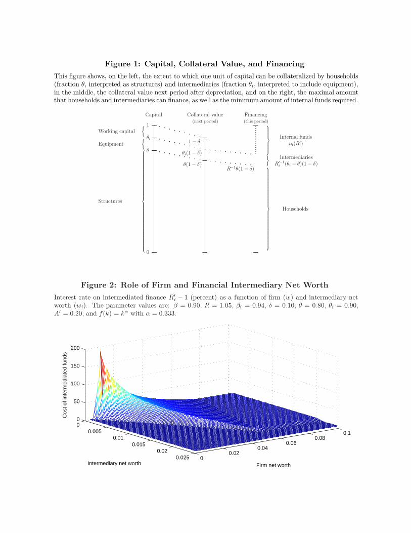
Figure 1: Capital, Collateral Value, and Financing

This figure shows, on the left, the extent to which one unit of capital can be collateralized by households(fraction θ, interpreted as structures) and intermediaries (fraction θi, interpreted to include equipment),in the middle, the collateral value next period after depreciation, and on the right, the maximal amountthat households and intermediaries can finance, as well as the minimum amount of internal funds required.

Capital Collateral value Financing(next period) (this period)

���������������

� � � � � � � � � �� � � � � � � � � �

� � � � � � � � � �

0

θ

θi

1

� � � � � � � � � �� � � � � � � � � �

θ(1 − δ)

θi(1 − δ)

1 − δ

R−1θ(1 − δ)

Working capital

Equipment

Structures

{

{

Internal funds℘i(R

′i)

IntermediariesR′−1

i (θi − θ)(1 − δ)

Households

}

Figure 2: Role of Firm and Financial Intermediary Net Worth

Interest rate on intermediated finance R′i − 1 (percent) as a function of firm (w) and intermediary net

worth (wi). The parameter values are: β = 0.90, R = 1.05, βi = 0.94, δ = 0.10, θ = 0.80, θi = 0.90,A′ = 0.20, and f(k) = kα with α = 0.333.

00.02

0.040.06

0.080.1

00.005

0.010.015

0.020.025

0

50

100

150

200

Firm net worthIntermediary net worth

Cos

t of i

nter

med

iate

d fu

nds

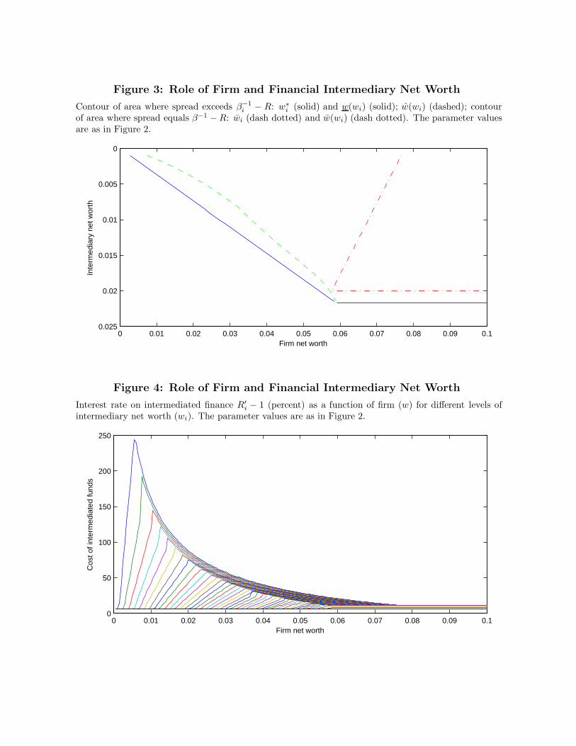
Figure 3: Role of Firm and Financial Intermediary Net Worth

Contour of area where spread exceeds β−1i − R: w∗

i (solid) and w(wi) (solid); w(wi) (dashed); contourof area where spread equals β−1 − R: wi (dash dotted) and w(wi) (dash dotted). The parameter valuesare as in Figure 2.

0 0.01 0.02 0.03 0.04 0.05 0.06 0.07 0.08 0.09 0.1

0

0.005

0.01

0.015

0.02

0.025

Firm net worth

Inte

rmed

iary

net

wor

th

Figure 4: Role of Firm and Financial Intermediary Net Worth

Interest rate on intermediated finance R′i − 1 (percent) as a function of firm (w) for different levels of

intermediary net worth (wi). The parameter values are as in Figure 2.

0 0.01 0.02 0.03 0.04 0.05 0.06 0.07 0.08 0.09 0.10

50

100

150

200

250

Firm net worth

Cos

t of i

nter

med

iate

d fu

nds

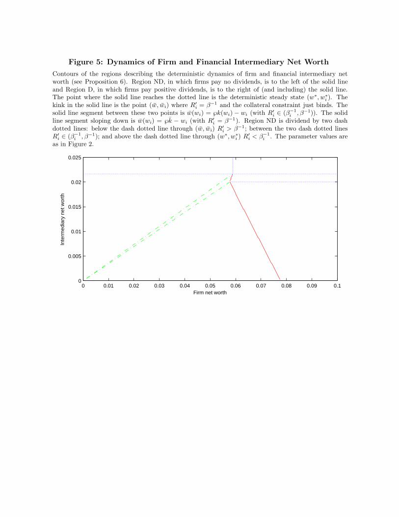
Figure 5: Dynamics of Firm and Financial Intermediary Net Worth

Contours of the regions describing the deterministic dynamics of firm and financial intermediary networth (see Proposition 6). Region ND, in which firms pay no dividends, is to the left of the solid lineand Region D, in which firms pay positive dividends, is to the right of (and including) the solid line.The point where the solid line reaches the dotted line is the deterministic steady state (w∗, w∗

i ). Thekink in the solid line is the point (w, wi) where R′

i = β−1 and the collateral constraint just binds. Thesolid line segment between these two points is w(wi) = ℘k(wi) − wi (with R′

i ∈ (β−1i , β−1)). The solid

line segment sloping down is w(wi) = ℘k − wi (with R′i = β−1). Region ND is dividend by two dash

dotted lines: below the dash dotted line through (w, wi) R′i > β−1; between the two dash dotted lines

R′i ∈ (β−1

i , β−1); and above the dash dotted line through (w∗, w∗i ) R′

i < β−1i . The parameter values are

as in Figure 2.

0 0.01 0.02 0.03 0.04 0.05 0.06 0.07 0.08 0.09 0.10

0.005

0.01

0.015

0.02

0.025

Firm net worth

Inte

rmed

iary

net

wor

th

Figure 6: Dynamics of Firm and Financial Intermediary Net Worth

This figures illustrates the deterministic dynamics starting from initial values of net worth w = 0.0222and wi = w′∗

i . Panel A traces out the path of firm and intermediary net worth in w vs. wi space withthe contours as in Figure 5. Panel B shows the evolution of the interest rate on intermediated finance(Panel B1), firm net worth (dashed) and intermediary net worth (solid) (cum dividends (higher) and exdividend (lower)) (Panel B2), intermediated lending to firms (solid) and households (dashed) (Panel B3),and investment (Panel B4). The parameter values are as in Figure 2 except that α = 0.8.

Panel A: Joint evolution of firm and intermediary net worth

0 0.05 0.1 0.15 0.2 0.250

0.02

0.04

0.06

0.08

0 1 2 3 45

67

890

678

910w∗i →

w∗i + d∗

i →

↑↑

w∗ w∗ + d∗

Firm net worth

Inte

rmed

iary

net

wor

th

Panel B: Interest rates, net worth, lending, and investment over time

0 5 10 15

1.04

1.06

1.08

1.1

1.12

1.14

← β−1

β−1i →

←R

Time

Panel B1. Cost of intermediated finance

0 5 10 150

0.1

0.2

0.3

w∗ →

w∗ + d∗ →

w∗i →w∗

i + d∗i →

Time

Panel B2. Firm and intermediary wealth

0 5 10 150

0.2

0.4

0.6

0.8k∗ →

k →

Time

Panel B4. Investment

0 5 10 150

0.02

0.04

0.06

0.08l′∗i →

Time

Panel B3. Intermediary lending

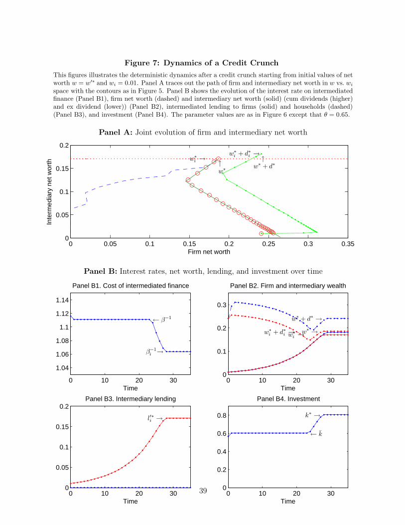
Figure 7: Dynamics of a Credit Crunch

This figures illustrates the deterministic dynamics after a credit crunch starting from initial values of networth w = w′∗ and wi = 0.01. Panel A traces out the path of firm and intermediary net worth in w vs. wi

space with the contours as in Figure 5. Panel B shows the evolution of the interest rate on intermediatedfinance (Panel B1), firm net worth (dashed) and intermediary net worth (solid) (cum dividends (higher)and ex dividend (lower)) (Panel B2), intermediated lending to firms (solid) and households (dashed)(Panel B3), and investment (Panel B4). The parameter values are as in Figure 6 except that θ = 0.65.

Panel A: Joint evolution of firm and intermediary net worth

0 0.05 0.1 0.15 0.2 0.25 0.3 0.350

0.05

0.1

0.15

0.2

w∗i →

w∗i + d∗

i →↑

↑

w∗ w∗ + d∗

Firm net worth

Inte

rmed

iary

net

wor

th

Panel B: Interest rates, net worth, lending, and investment over time

0 10 20 30

1.04

1.06

1.08

1.1

1.12

1.14

← β−1

β−1i →

Time

Panel B1. Cost of intermediated finance

0 10 20 300

0.1

0.2

0.3

w∗ →

w∗ + d∗ →

w∗i →w∗

i + d∗i →

Time

Panel B2. Firm and intermediary wealth

0 10 20 300

0.05

0.1

0.15

0.2

l′∗i →

Time

Panel B3. Intermediary lending

0 10 20 300

0.2

0.4

0.6

0.8 k∗ →

← k

Time

Panel B4. Investment

39