finance 30210: managerial economics strategic pricing techniques
TRANSCRIPT
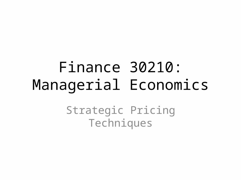
Finance 30210: Managerial Economics
Strategic Pricing Techniques
Market Structures
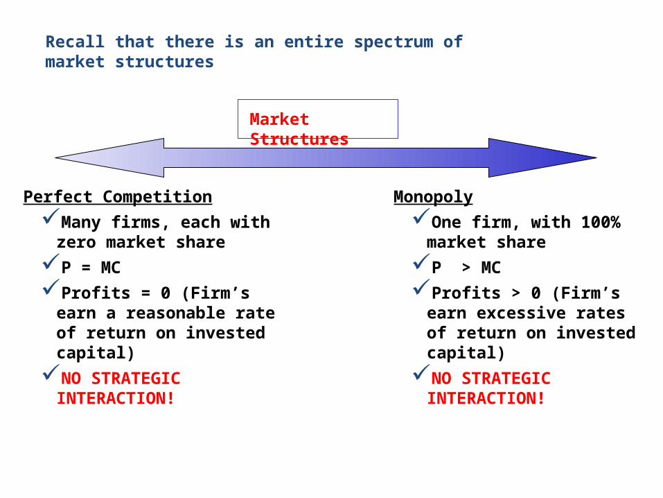
Recall that there is an entire spectrum of market structures
Perfect Competition
Many firms, each with zero market share
P = MC
Profits = 0 (Firm’s earn a reasonable rate of return on invested capital)
NO STRATEGIC INTERACTION!
Monopoly
One firm, with 100% market share
P > MC
Profits > 0 (Firm’s earn excessive rates of return on invested capital)
NO STRATEGIC INTERACTION!
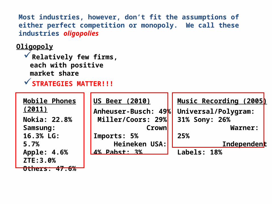
Most industries, however, don’t fit the assumptions of either perfect competition or monopoly. We call these industries oligopolies
Oligopoly
Relatively few firms, each with positive market share
STRATEGIES MATTER!!!
Mobile Phones (2011)
Nokia: 22.8% Samsung: 16.3% LG: 5.7% Apple: 4.6% ZTE:3.0% Others: 47.6%
US Beer (2010)
Anheuser-Busch: 49% Miller/Coors: 29% Crown Imports: 5% Heineken USA: 4% Pabst: 3%
Music Recording (2005)
Universal/Polygram: 31% Sony: 26% Warner: 25% Independent Labels: 18%
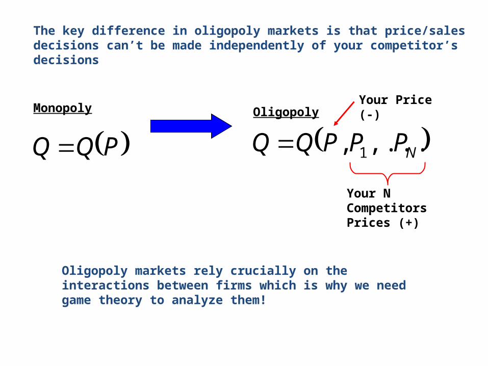
The key difference in oligopoly markets is that price/sales decisions can’t be made independently of your competitor’s decisions
Monopoly
PQQ Oligopoly
NPPPQQ ,..., 1
Your Price (-)
Your N Competitors Prices (+)
Oligopoly markets rely crucially on the interactions between firms which is why we need game theory to analyze them!
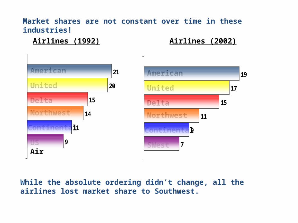
Market shares are not constant over time in these industries!
9
11
14
15
20
21
Airlines (1992) Airlines (2002)
American
Northwest
Delta
United
Continental
US Air 7
9
11
15
17
19American
United
Delta
Northwest
Continental
SWest
While the absolute ordering didn’t change, all the airlines lost market share to Southwest.
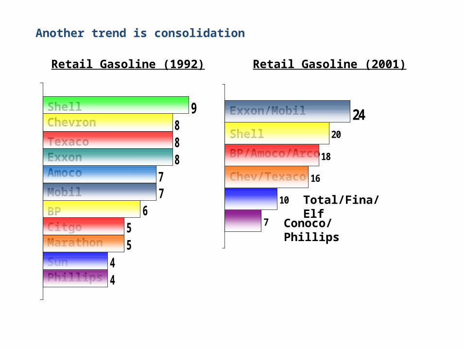
Another trend is consolidation
44
55
677
888
9
Retail Gasoline (1992) Retail Gasoline (2001)
Shell
ExxonTexaco
Chevron
Amoco
Mobil
7
10
16
18
20
24Exxon/Mobil
Shell
BP/Amoco/Arco
Chev/Texaco
Conoco/PhillipsCitgoBP
Marathon
SunPhillips
Total/Fina/Elf

Jake
Clyde
Confess
Don’t Confess
Confess
-4 -4 0 -8
Don’t Confess
-8 0 -1 -1
The prisoner’s dilemma game is used to describe circumstances where competition forces sub-optimal outcomes
Recall the prisoners dilemma game…
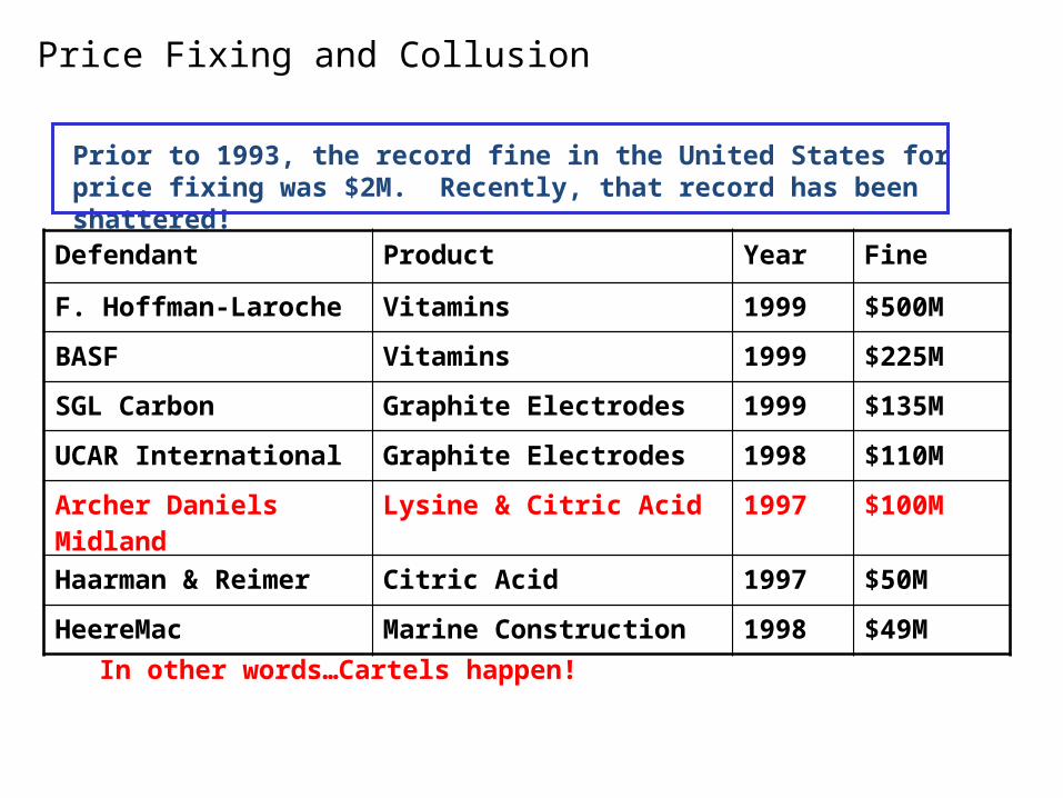
Price Fixing and Collusion
Prior to 1993, the record fine in the United States for price fixing was $2M. Recently, that record has been shattered!
Defendant Product Year Fine
F. Hoffman-Laroche Vitamins 1999 $500M
BASF Vitamins 1999 $225M
SGL Carbon Graphite Electrodes 1999 $135M
UCAR International Graphite Electrodes 1998 $110M
Archer Daniels Midland Lysine & Citric Acid 1997 $100M
Haarman & Reimer Citric Acid 1997 $50M
HeereMac Marine Construction 1998 $49M
In other words…Cartels happen!
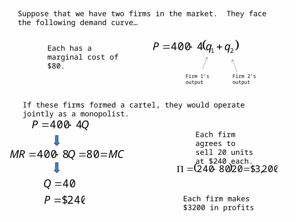
Suppose that we have two firms in the market. They face the following demand curve…
214400 qqP
Firm 1’s output Firm 2’s output
Each has a marginal cost of $80.
If these firms formed a cartel, they would operate jointly as a monopolist.
QP 4400
MCQMR 808400
240$
40
P
Q
Each firm agrees to sell 20 units at $240 each.
200,3$2080240
Each firm makes $3200 in profits
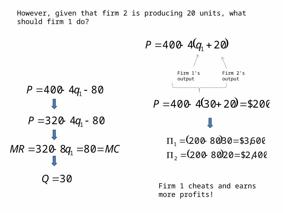
However, given that firm 2 is producing 20 units, what should firm 1 do?
204400 1 qP
Firm 1’s output Firm 2’s output
804400 1 qP
804320 1 qP
MCqMR 808320 1
30Q
200$20304400 P
600,3$30802001 400,2$20802002
Firm 1 cheats and earns more profits!
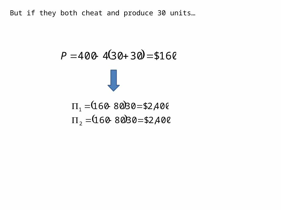
But if they both cheat and produce 30 units…
160$30304400 P
400,2$30801601 400,2$30801602
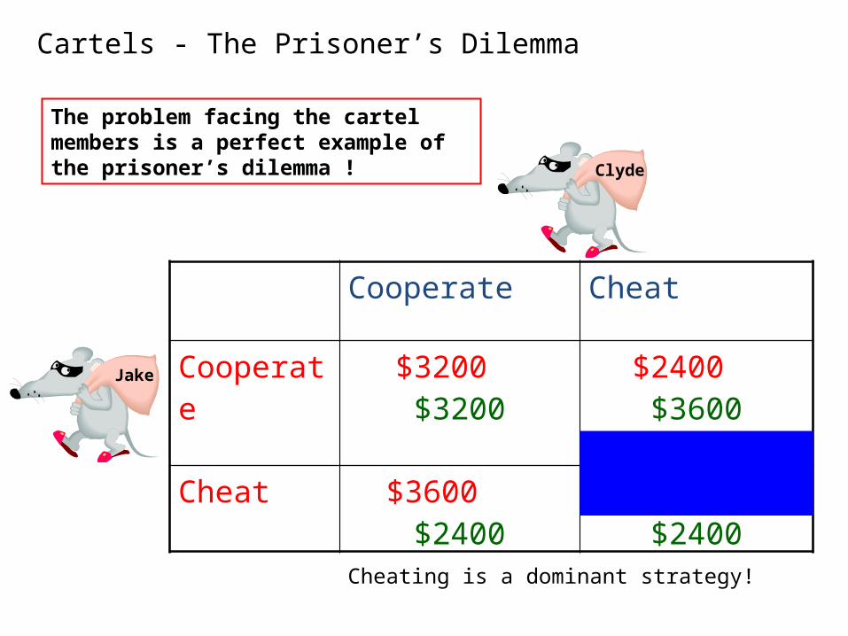
Cartels - The Prisoner’s Dilemma
Jake
Clyde
Cooperate Cheat
Cooperate $3200 $3200 $2400 $3600
Cheat $3600 $2400 $2400 $2400
The problem facing the cartel members is a perfect example of the prisoner’s dilemma !
Cheating is a dominant strategy!
Cartel Formation
While it is clearly in each firm’s best interest to join the cartel, there are a couple problems:
With the high monopoly markup, each firm has the incentive to cheat and overproduce. If every firm cheats, the price falls and the cartel breaks down
Cartels are generally illegal which makes enforcement difficult!
Note that as the number of cartel members increases the benefits increase, but more members makes enforcement even more difficult!
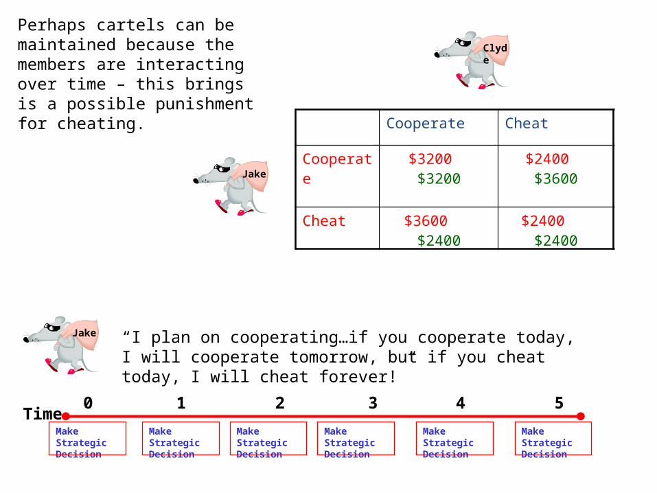
Perhaps cartels can be maintained because the members are interacting over time – this brings is a possible punishment for cheating.
Time0 1 2 3 4 5
Make Strategic Decision
Jake
Clyde
Make Strategic Decision
Make Strategic Decision
Make Strategic Decision
Make Strategic Decision
Make Strategic Decision
Jake “I plan on cooperating…if you cooperate today, I will cooperate tomorrow, but if you cheat today, I will cheat forever!”
Cooperate Cheat
Cooperate $3200 $3200 $2400 $3600
Cheat $3600 $2400 $2400 $2400
Time0 1 2 3 4 5
Make Strategic Decision
Make Strategic Decision
Make Strategic Decision
Make Strategic Decision
Make Strategic Decision
Make Strategic Decision
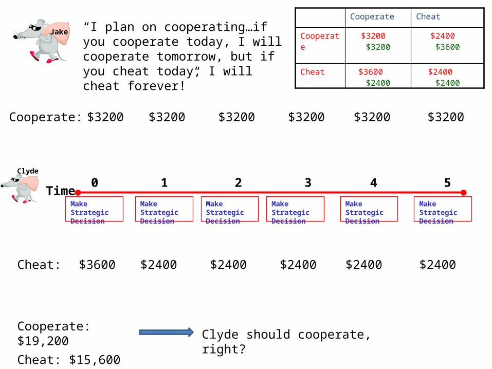
Jake “I plan on cooperating…if you cooperate today, I will cooperate tomorrow, but if you cheat today, I will cheat forever!”
Clyde
Cooperate:
Cheat:
$3200 $3200 $3200 $3200 $3200 $3200
$3600 $2400 $2400 $2400 $2400 $2400
Cooperate: $19,200
Cheat: $15,600Clyde should cooperate, right?
Cooperate Cheat
Cooperate $3200 $3200 $2400 $3600
Cheat $3600 $2400 $2400 $2400
Jake Clyde
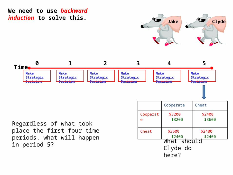
We need to use backward induction to solve this.
Time0 1 2 3 4 5
Make Strategic Decision
Make Strategic Decision
Make Strategic Decision
Make Strategic Decision
Make Strategic Decision
Make Strategic Decision
What should Clyde do here?
Regardless of what took place the first four time periods, what will happen in period 5?
Cooperate Cheat
Cooperate $3200 $3200 $2400 $3600
Cheat $3600 $2400 $2400 $2400

Jake Clyde
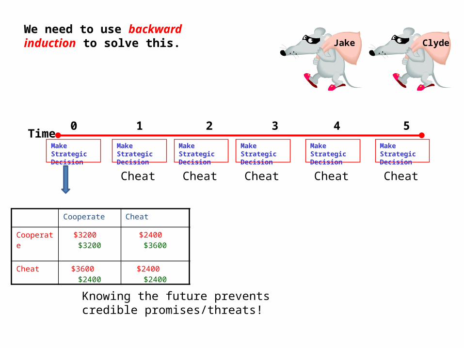
We need to use backward induction to solve this.
Time0 1 2 3 4 5
Make Strategic Decision
Make Strategic Decision
Make Strategic Decision
Make Strategic Decision
Make Strategic Decision
Make Strategic Decision
What should Clyde do here?
Cheat
Given what happens in period 5, what should happen in period 4?
Cooperate Cheat
Cooperate $3200 $3200 $2400 $3600
Cheat $3600 $2400 $2400 $2400
Jake Clyde
We need to use backward induction to solve this.
Time0 1 2 3 4 5
Make Strategic Decision
Make Strategic Decision
Make Strategic Decision
Make Strategic Decision
Make Strategic Decision
Make Strategic Decision
Knowing the future prevents credible promises/threats!
Cheat Cheat Cheat Cheat Cheat
Cooperate Cheat
Cooperate $3200 $3200 $2400 $3600
Cheat $3600 $2400 $2400 $2400
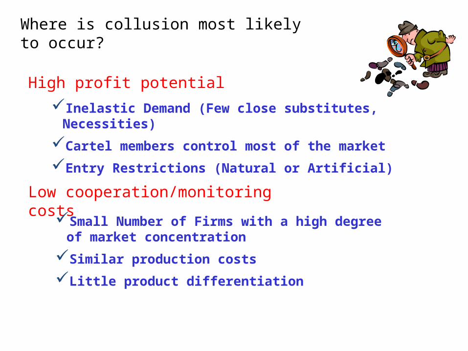
Where is collusion most likely to occur?
High profit potential
Inelastic Demand (Few close substitutes, Necessities)
Cartel members control most of the market
Entry Restrictions (Natural or Artificial)
Low cooperation/monitoring costs
Small Number of Firms with a high degree of market concentration
Similar production costs
Little product differentiation
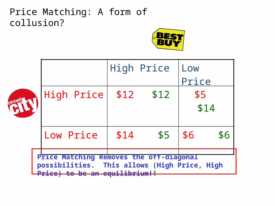
Price Matching: A form of collusion?
High Price Low Price
High Price $12 $12 $5 $14
Low Price $14 $5 $6 $6
Price Matching Removes the off-diagonal possibilities. This allows (High Price, High Price) to be an equilibrium!!
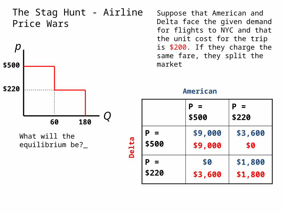
The Stag Hunt - Airline Price Wars
p
Q
$500
$220
60 180
Suppose that American and Delta face the given demand for flights to NYC and that the unit cost for the trip is $200. If they charge the same fare, they split the market
P = $500 P = $220
P = $500 $9,000$9,000
$3,600$0
P = $220 $0$3,600
$1,800$1,800
American
Del
taWhat will the equilibrium be?

The Airline Price Wars
P = $500 P = $220
P = $500 $9,000$9,000
$3,600$0
P = $220 $0$3,600
$1,800$1,800
American
Del
ta
If American follows a strategy of charging $500 all the time, Delta’s best response is to also charge $500 all the time
If American follows a strategy of charging $220 all the time, Delta’s best response is to also charge $220 all the time
This game has multiple equilibria and the result depends critically on each company’s beliefs about the other company’s strategy
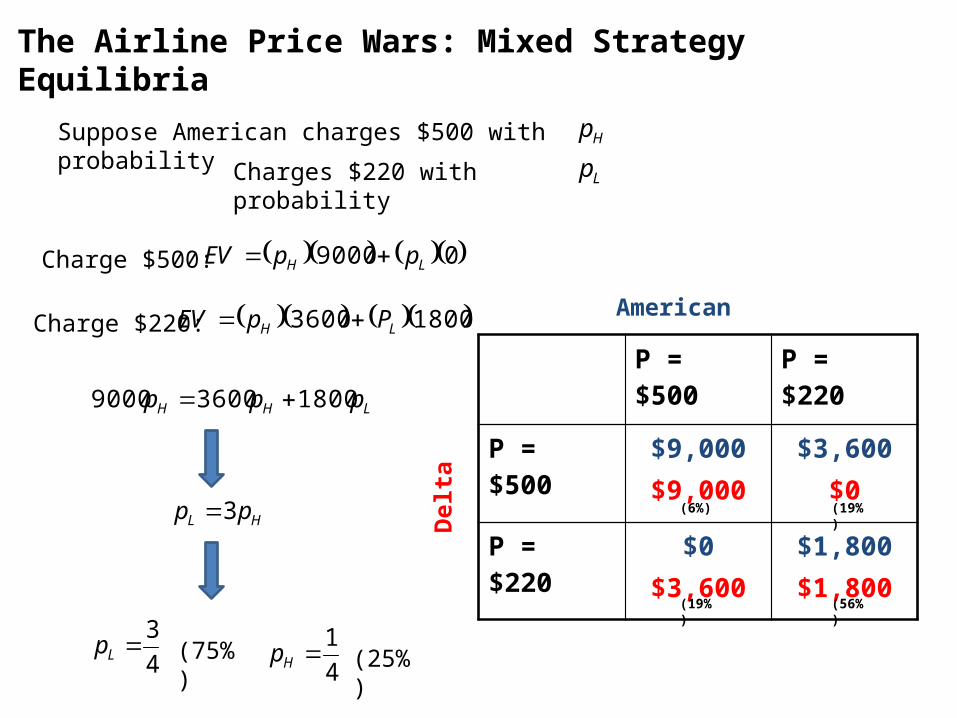
The Airline Price Wars: Mixed Strategy Equilibria
P = $500 P = $220
P = $500 $9,000$9,000
$3,600$0
P = $220 $0$3,600
$1,800$1,800
American
Del
ta
Charge $500: 09000 LH ppEV
Charge $220: 18003600 LH PpEV
Suppose American charges $500 with probability Hp
Charges $220 with probability Lp
LHH ppp 180036009000
HL pp 3
4
3Lp
4
1Hp(75%) (25%)
(56%)(19%)
(19%)(6%)
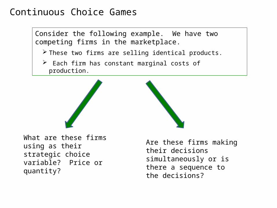
Continuous Choice Games
Consider the following example. We have two competing firms in the marketplace.
These two firms are selling identical products.
Each firm has constant marginal costs of production.
What are these firms using as their strategic choice variable? Price or quantity?
Are these firms making their decisions simultaneously or is there a sequence to the decisions?
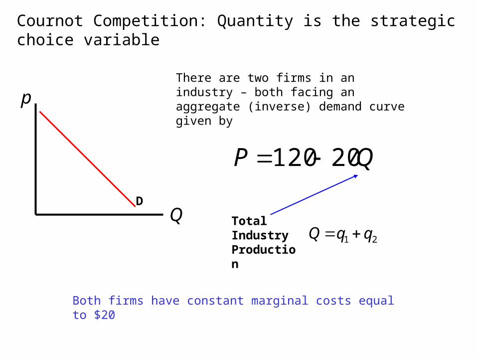
Cournot Competition: Quantity is the strategic choice variable
p
QD
There are two firms in an industry – both facing an aggregate (inverse) demand curve given by
Total Industry Production
Both firms have constant marginal costs equal to $20
21 qqQ
QP 20120

Consider the following scenario…We call this Cournot competition
Two manufacturers choose a production target
Q2
Q1
P
Q1 + Q2
Q
S
D
P*
A centralized market determines the market price based on available supply and current demand
Two manufacturers earn profits based off the market price
Profit = P*Q1 - TC
Profit = P*Q2 - TC
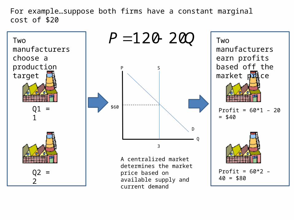
For example…suppose both firms have a constant marginal cost of $20
Two manufacturers choose a production target
Q2 = 2
Q1 = 1
P
3
Q
S
D
$60
A centralized market determines the market price based on available supply and current demand
Two manufacturers earn profits based off the market price
Profit = 60*1 – 20 = $40
Profit = 60*2 – 40 = $80
QP 20120
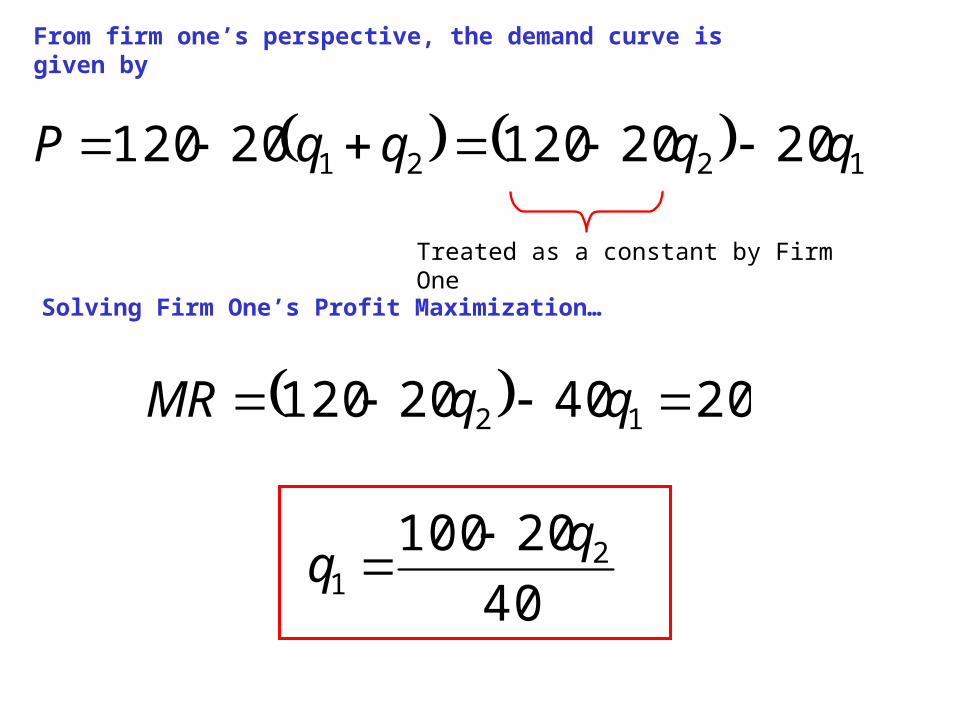
From firm one’s perspective, the demand curve is given by
1221 202012020120 qqqqP
Treated as a constant by Firm One
Solving Firm One’s Profit Maximization…
204020120 12 qqMR
40
20100 21
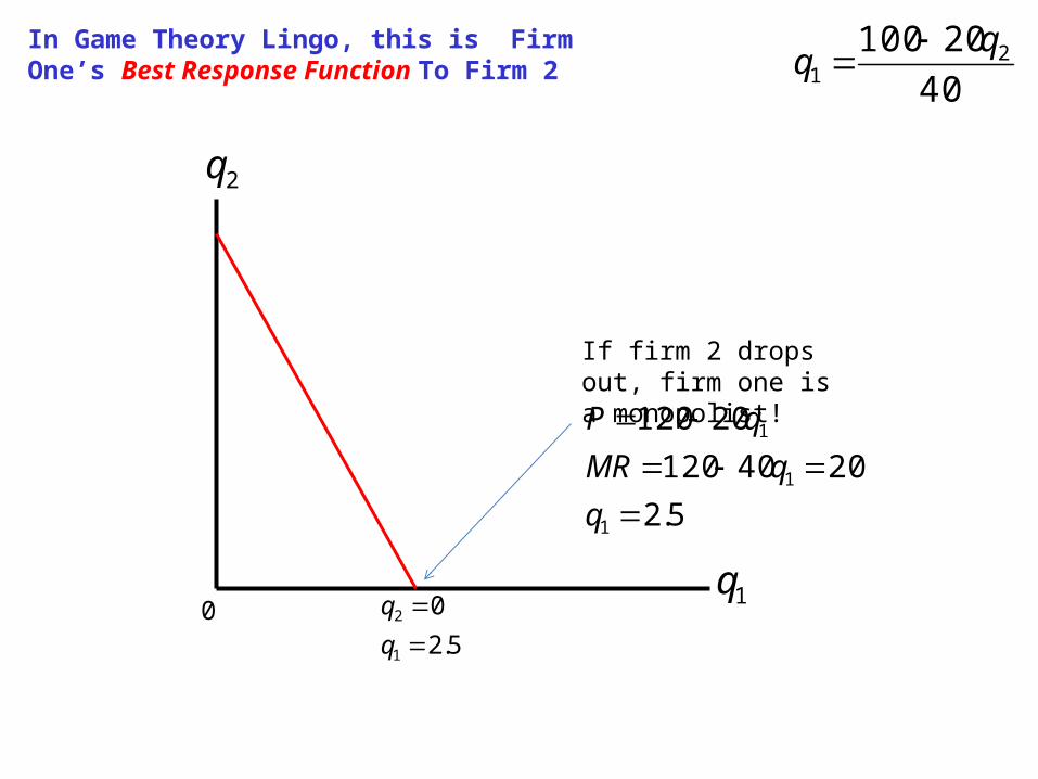
In Game Theory Lingo, this is Firm One’s Best Response Function To Firm 2
1q
2q
40
20100 21
05.2
0
1
2
q
q
If firm 2 drops out, firm one is a monopolist!
5.2
2040120
20120
1
1
1
q
qMR
qP
1q
2q
40
20100 21
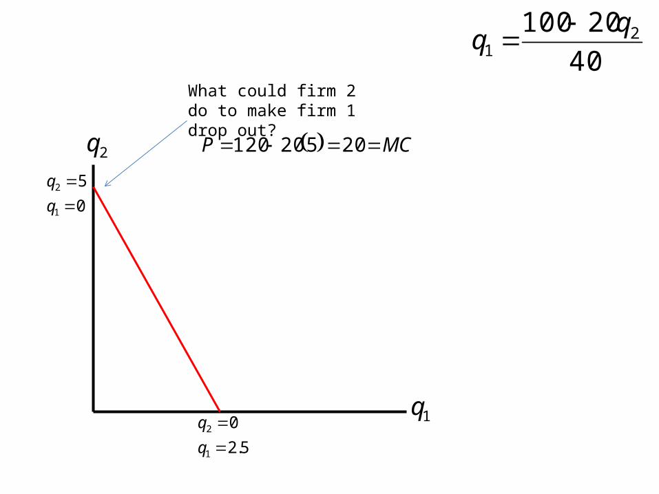
What could firm 2 do to make firm 1 drop out?
5.2
0
1
2
q
q
0
5
1
2
q
q
MCP 20520120
1q
2q 40
20100 21
5.2
0
1
2
q
q
0
5
1
2
q
q
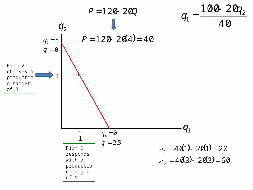
3
1
Firm 2 chooses a production target of 3
Firm 1 responds with a production target of 1
QP 20120
40420120 P
60320340
20120140
2
1
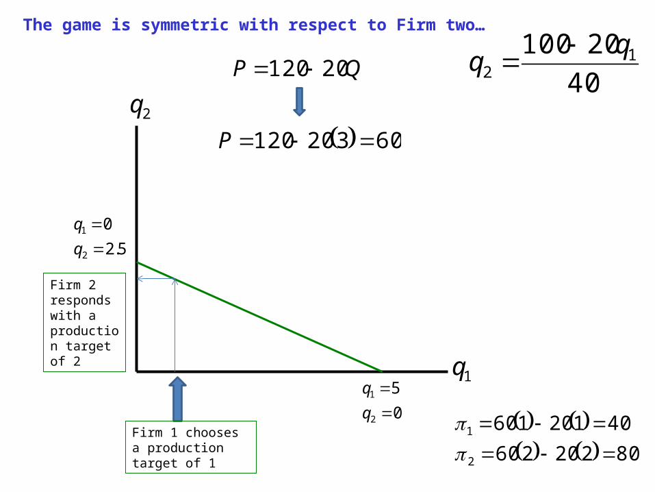
The game is symmetric with respect to Firm two…
1q
2q40
20100 12
5.2
0
2
1
q
q
0
5
2
1
q
q
Firm 1 chooses a production target of 1
Firm 2 responds with a production target of 2
QP 20120
60320120 P
80220260
40120160
2
1
1q
2q
Firm 1
Firm 2
67.1*
1q
67.1*2 q
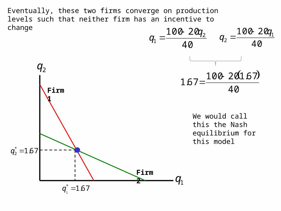
Eventually, these two firms converge on production levels such that neither firm has an incentive to change
40
20100 12
40
20100 21
40
67.12010067.1
We would call this the Nash equilibrium for this model
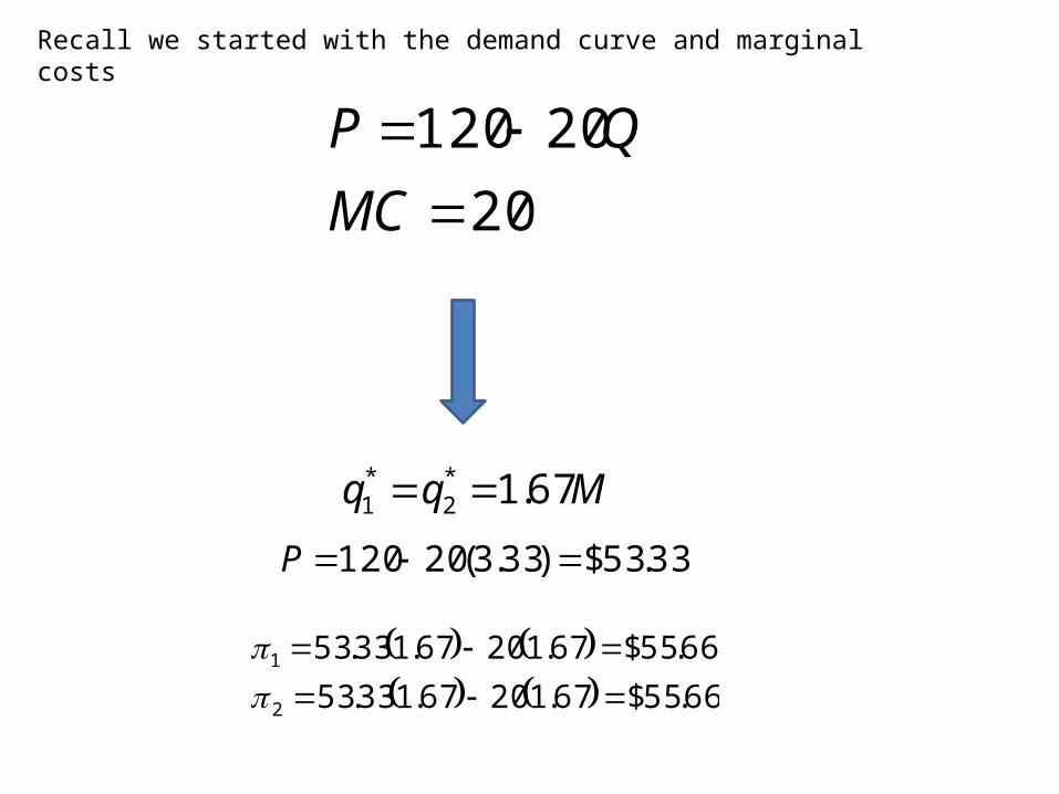
Recall we started with the demand curve and marginal costs
20
20120
MC
QP
Mqq 67.1*2
*1
33.53$)33.3(20120 P
66.55$67.12067.133.53
66.55$67.12067.133.53
2
1
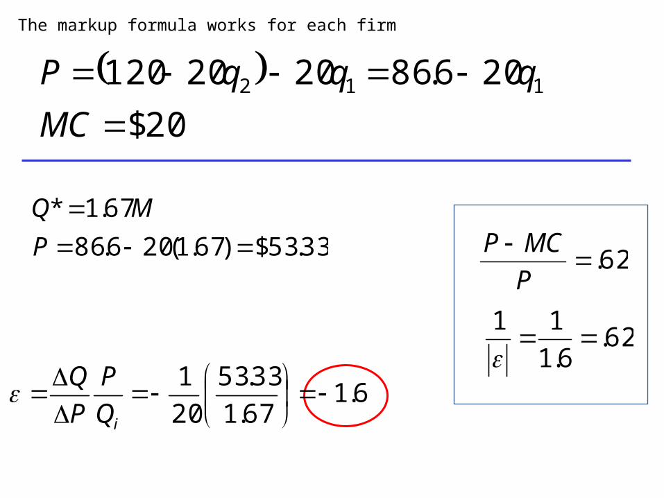
The markup formula works for each firm
33.53$)67.1(206.86
67.1*
P
MQ
62.P
MCP
6.167.1
33.53
20
1
iQ
P
P
Q
62.6.1
11
20$
206.862020120 112
MC
qqqP
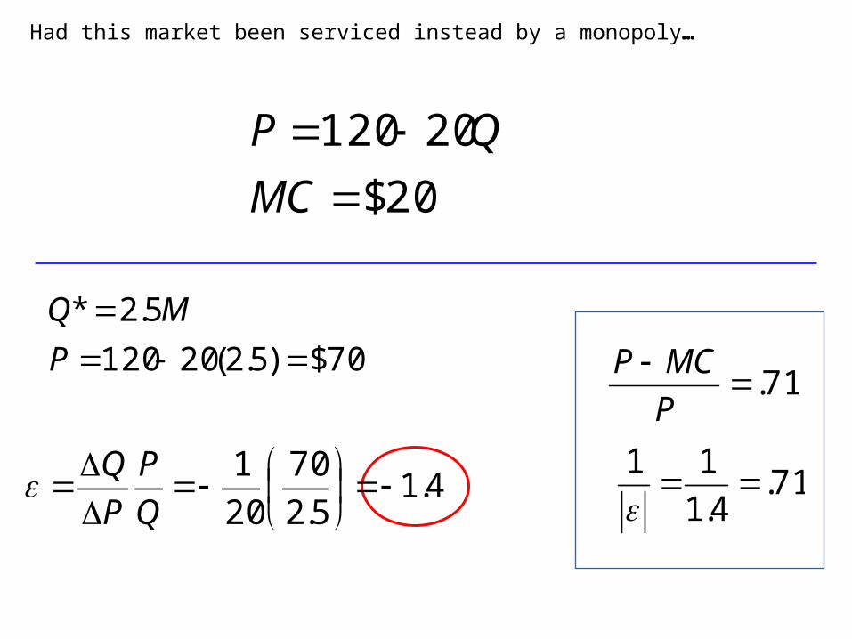
Had this market been serviced instead by a monopoly…
70$)5.2(20120
5.2*
P
MQ
20$
20120
MC
QP
4.15.2
70
20
1
Q
P
P
Q
71.P
MCP
71.4.1
11
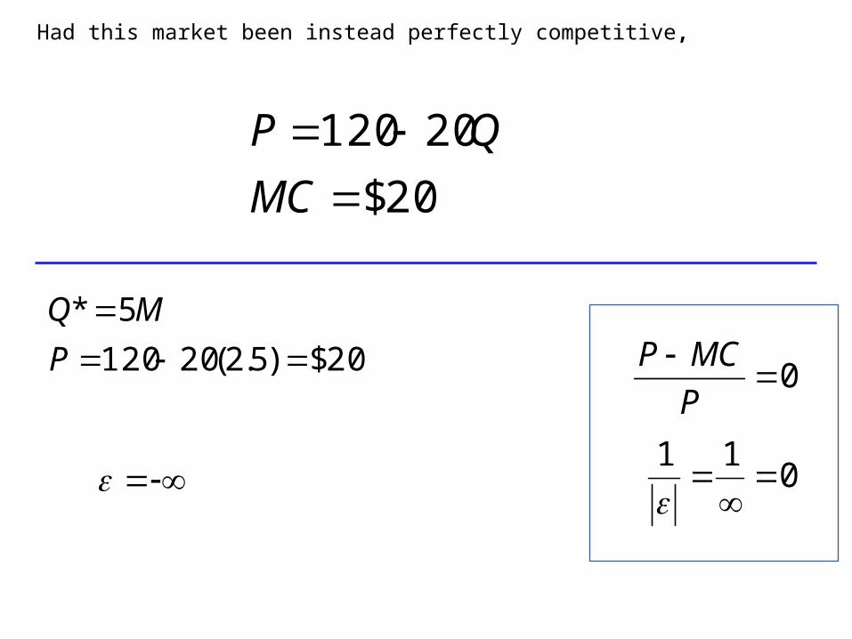
Had this market been instead perfectly competitive,
20$)5.2(20120
5*
P
MQ
20$
20120
MC
QP
0P
MCP
011
20$
20120
MC
QP
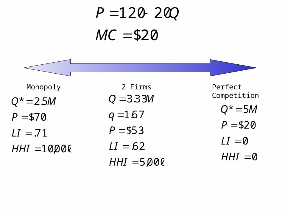
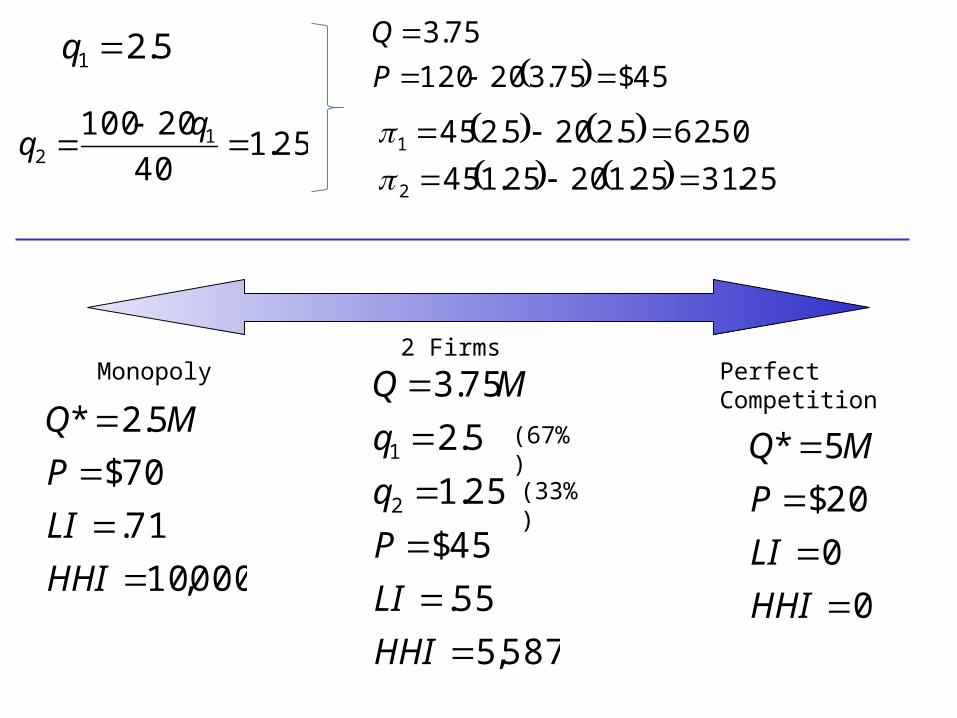
Monopoly
000,10
71.
70$
5.2*
HHI
LI
P
MQ
Perfect Competition
0
0
20$
5*
HHI
LI
P
MQ
2 Firms
000,5
62.
53$
67.1
33.3
HHI
LI
P
q
MQ
20$
20120
MC
QP
p
QD
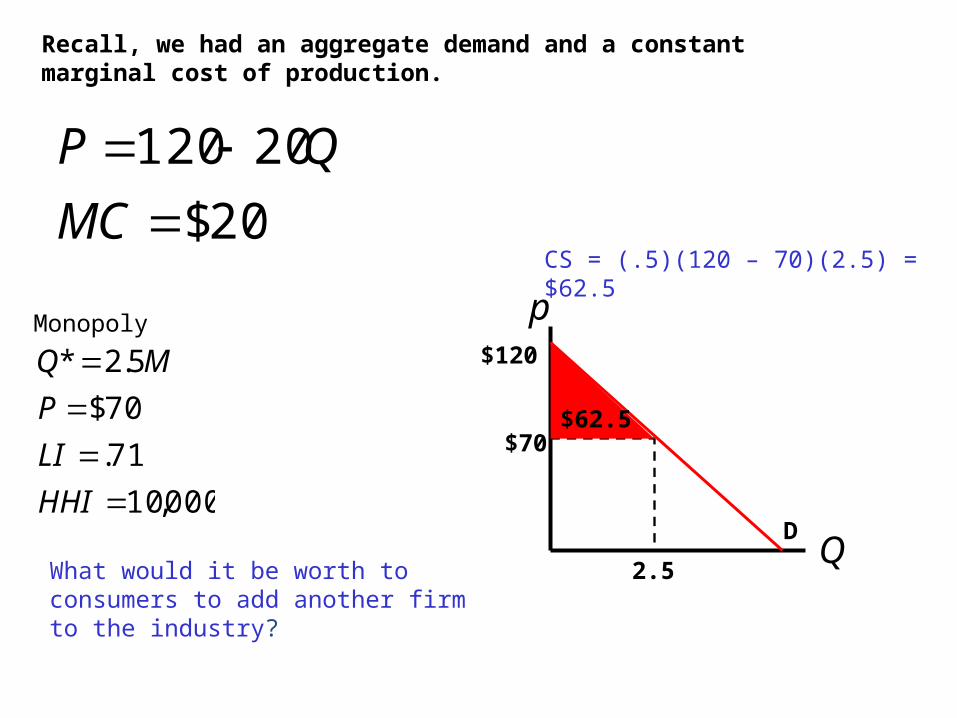
$70
2.5
CS = (.5)(120 – 70)(2.5) = $62.5
$62.5
What would it be worth to consumers to add another firm to the industry?
Recall, we had an aggregate demand and a constant marginal cost of production.
Monopoly$120
000,10
71.
70$
5.2*
HHI
LI
P
MQ
20$
20120
MC
QP
p
QD
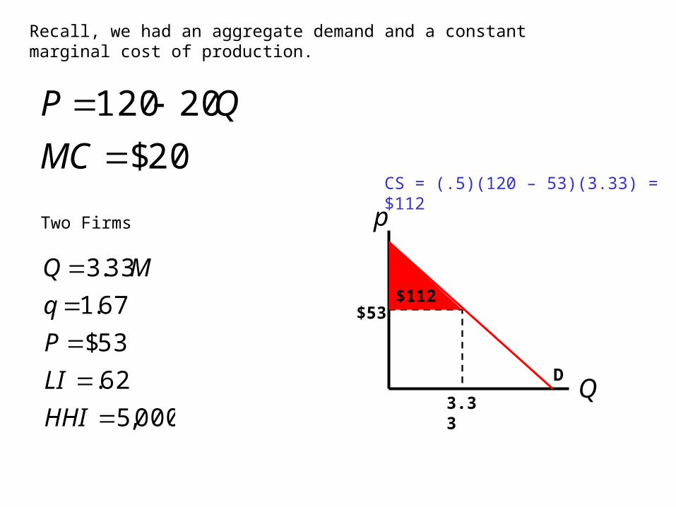
$53
3.33
CS = (.5)(120 – 53)(3.33) = $112
$112
Recall, we had an aggregate demand and a constant marginal cost of production.
000,5
62.
53$
67.1
33.3
HHI
LI
P
q
MQ
Two Firms
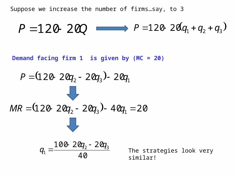
Suppose we increase the number of firms…say, to 3
QP 20120
Demand facing firm 1 is given by (MC = 20)
32120120 qqqP
132 202020120 qqqP
20402020120 132 qqqMR
40
2020100 321
qqq
The strategies look very similar!
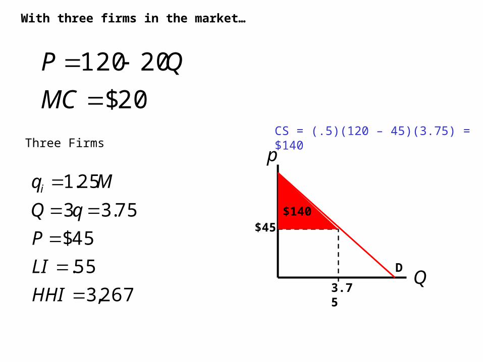
20$
20120
MC
QP
p
QD
$45
3.75
CS = (.5)(120 – 45)(3.75) = $140
$140
267,3
55.
45$
75.33
25.1
HHI
LI
P
Mqi
With three firms in the market…
Three Firms
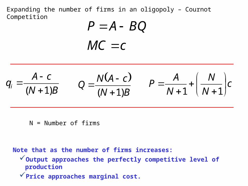
Expanding the number of firms in an oligopoly – Cournot Competition
BN
cAqi )1(
BN
cANQ
)1(
cN
N
N
AP
11
Note that as the number of firms increases:
Output approaches the perfectly competitive level of production
Price approaches marginal cost.
cMC
BQAP
N = Number of firms
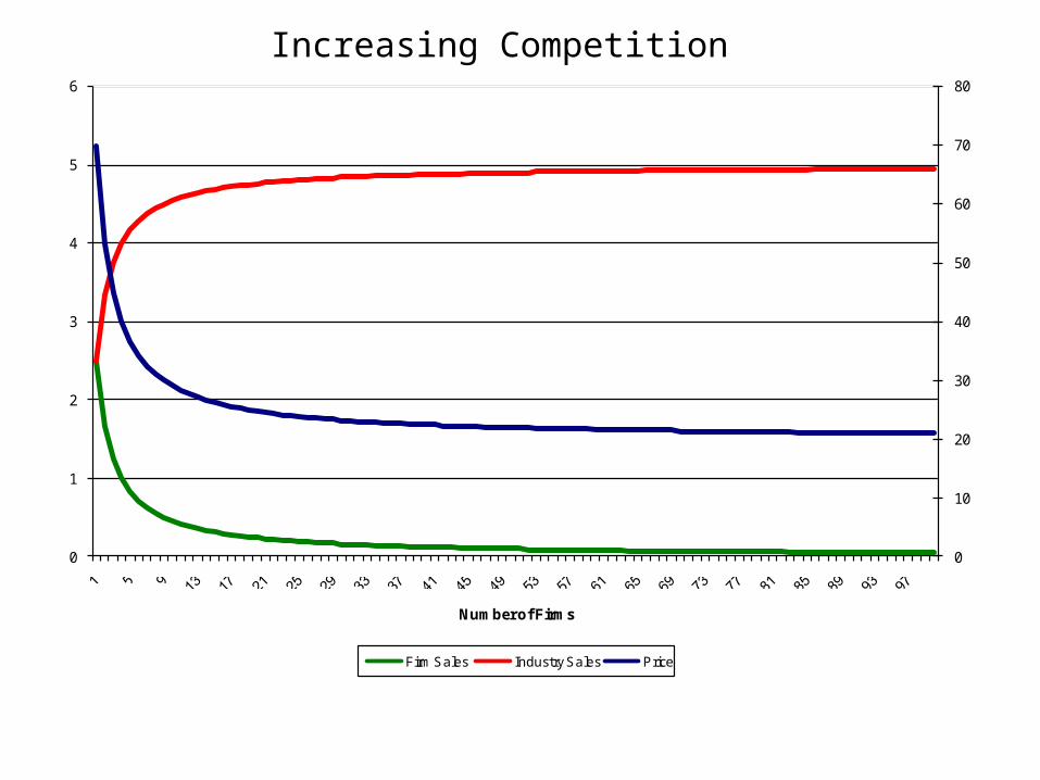
0
10
20
30
40
50
60
70
80
0
1
2
3
4
5
6
Number of Firms
Firm Sales Industry Sales Price
Increasing Competition
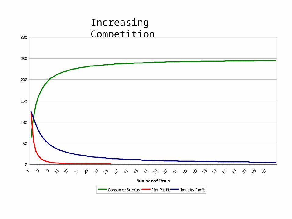
Increasing Competition
0
50
100
150
200
250
300
Number of Firms
Consumer Surplus Firm Profit Industry Profit
1q
2q
Firm 1
Firm 2
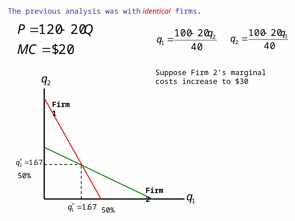
The previous analysis was with identical firms.
67.1*2 q
67.1*1 q
Suppose Firm 2’s marginal costs increase to $30
20$
20120
MC
QP40
20100 12
40
20100 21
50%
50%
1q
2q
Firm 2
67.1*2 q
67.1*1 q
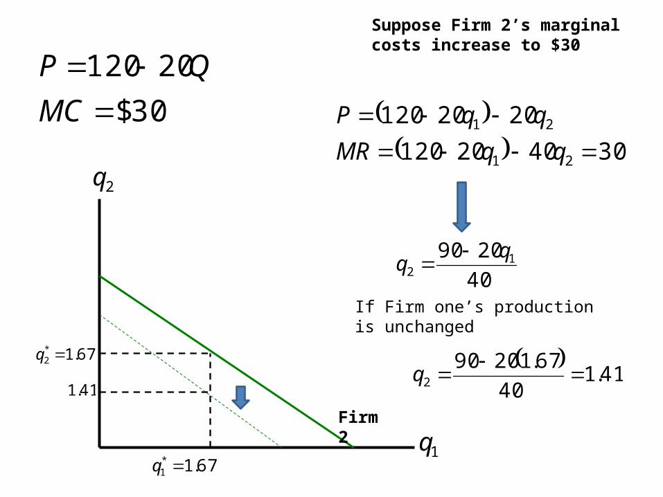
30$
20120
MC
QP
304020120
2020120
21
21
qqMR
qqP
Suppose Firm 2’s marginal costs increase to $30
40
2090 12
If Firm one’s production is unchanged
41.1
40
67.120902
q
41.1
1q
2q
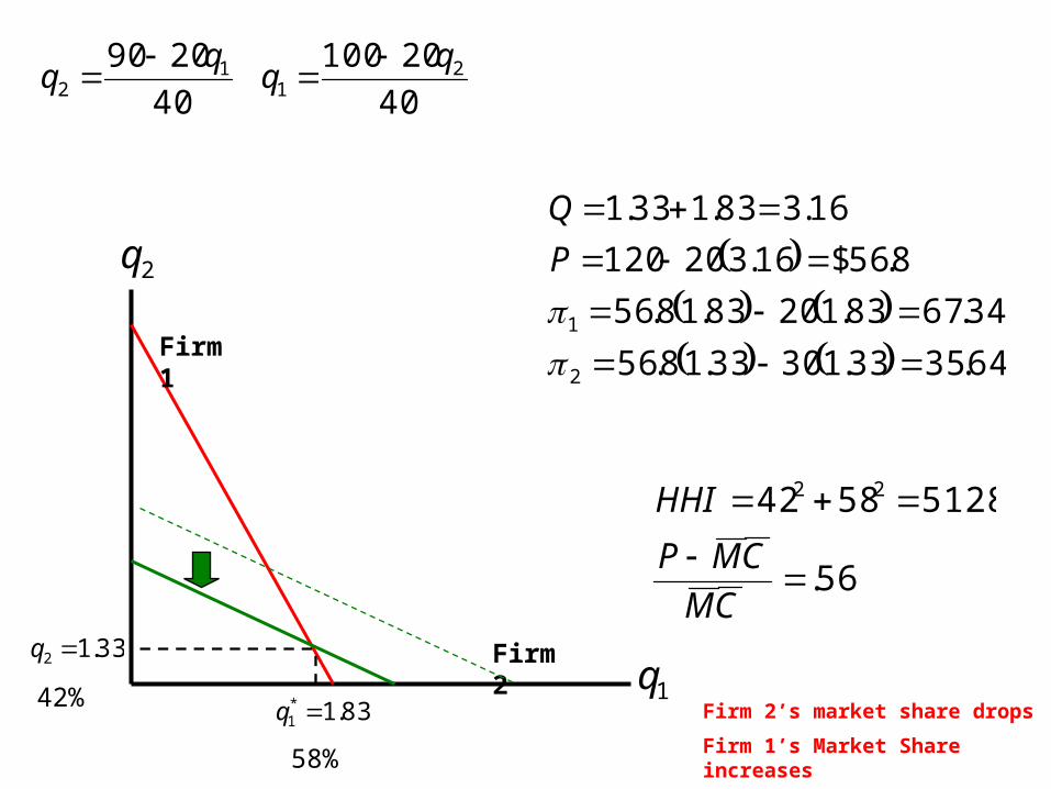
Firm 1
Firm 233.12 q
83.1*1 q Firm 2’s market share drops
Firm 1’s Market Share increases
42%
58%
40
2090 12
40
20100 21
64.3533.13033.18.56
34.6783.12083.18.56
8.56$16.320120
16.383.133.1
2
1
P
Q
56.
51285842 22
CM
CMP
HHI

Market Concentration and Profitability
N
iiqBAP
1
Industry Demand
is
P
MCP
000,10
HHI
P
MCP
The Lerner index for Firm i is related to Firm i’s market share and the elasticity of industry demand
The Average Lerner index for the industry is related to the HHI and the elasticity of industry demand
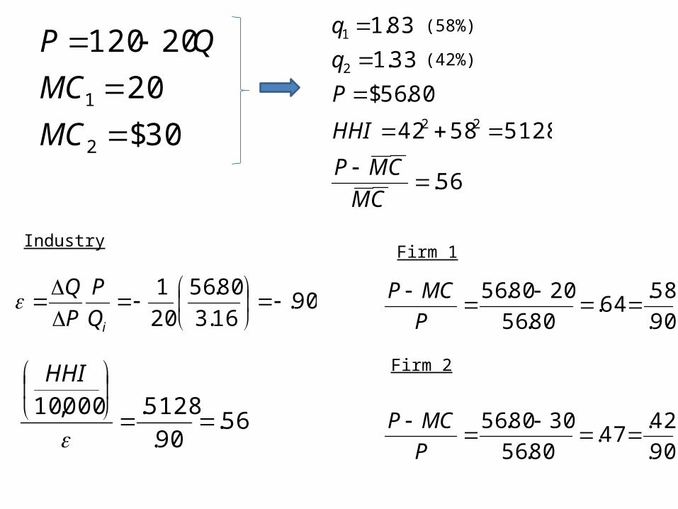
30$
20
20120
2
1
MC
MC
QP
56.
51285842
80.56$
33.1
83.1
22
2
1
CM
CMP
HHI
P
q
q
(42%)
(58%)
Industry
56.90.
5128.000,10
HHI
90.16.3
80.56
20
1
iQ
P
P
Q
Firm 1
Firm 2
90.
58.64.
80.56
2080.56
P
MCP
90.
42.47.
80.56
3080.56
P
MCP
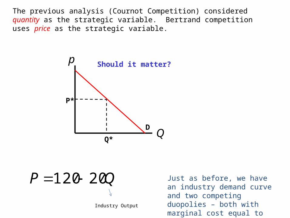
The previous analysis (Cournot Competition) considered quantity as the strategic variable. Bertrand competition uses price as the strategic variable.
p
QD
Q*
P*
Should it matter?
QP 20120 Just as before, we have an industry demand curve and two competing duopolies – both with marginal cost equal to $20.Industry Output
1qD
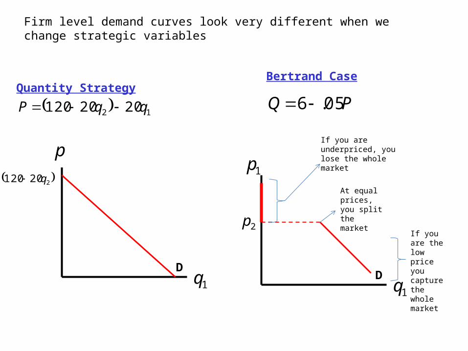
12 2020120 qqP PQ 05.6 Quantity Strategy
1p
1qD
Bertrand Case
220120 q
p
2p
Firm level demand curves look very different when we change strategic variables
If you are underpriced, you lose the whole market
If you are the low price you capture the whole market
At equal prices, you split the market
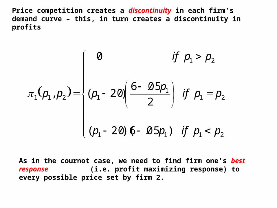
Price competition creates a discontinuity in each firm’s demand curve – this, in turn creates a discontinuity in profits
2111
211
1
21
211
)05.6)(20(
2
05.6)20(
0
,
ppifpp
ppifp
p
ppif
pp
As in the cournot case, we need to find firm one’s best response (i.e. profit maximizing response) to every possible price set by firm 2.

Firm One’s Best Response Function
mpp 2
Case #1: Firm 2 sets a price above the pure monopoly price:
220 pCase #3: Firm 2 sets a price below marginal cost
202 ppm
Case #2: Firm 2 sets a price between the monopoly price and marginal cost
mpp 1
21 pp
21 pp
2pc Case #4: Firm 2 sets a price equal to marginal cost
cpp 21
What’s the Nash equilibrium of this game?
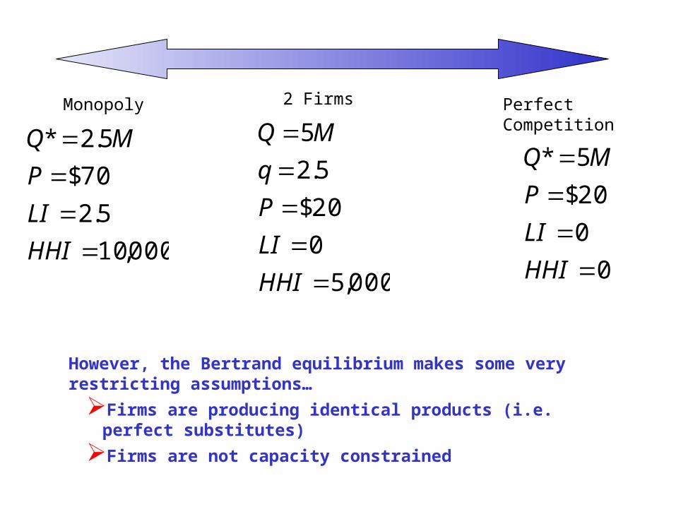
However, the Bertrand equilibrium makes some very restricting assumptions…
Firms are producing identical products (i.e. perfect substitutes)
Firms are not capacity constrained
Monopoly
000,10
5.2
70$
5.2*
HHI
LI
P
MQ
Perfect Competition
0
0
20$
5*
HHI
LI
P
MQ
2 Firms
000,5
0
20$
5.2
5
HHI
LI
P
q
MQ
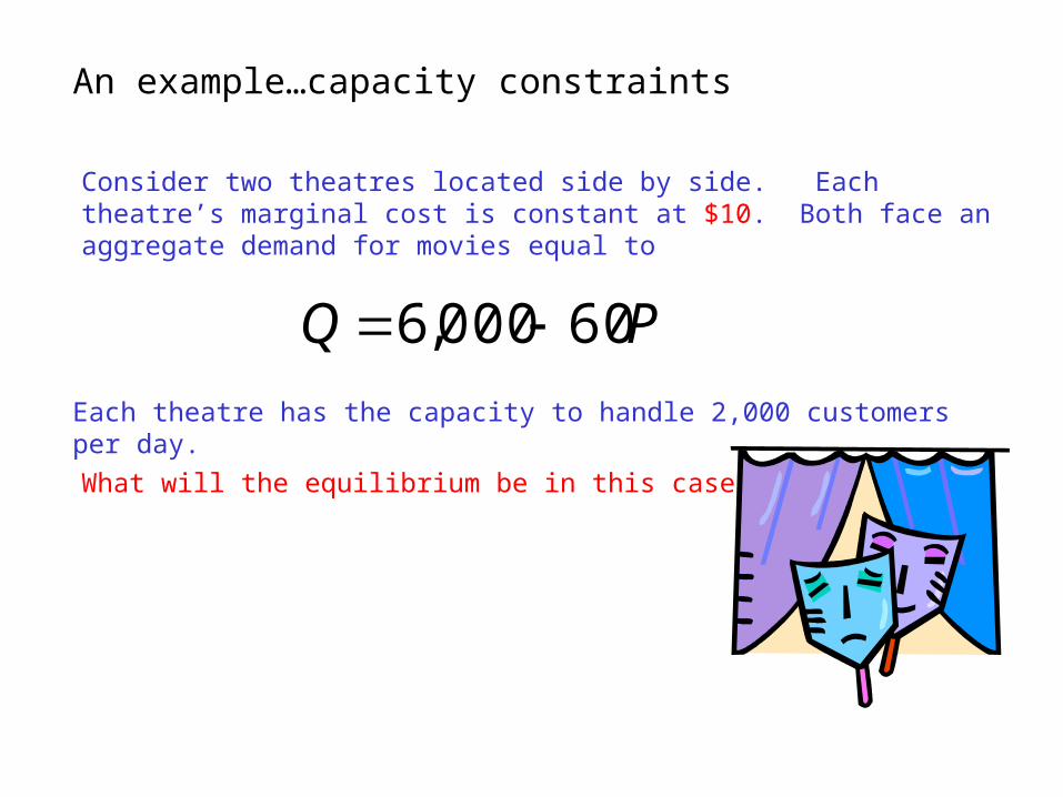
An example…capacity constraints
Consider two theatres located side by side. Each theatre’s marginal cost is constant at $10. Both face an aggregate demand for movies equal to
PQ 60000,6 Each theatre has the capacity to handle 2,000 customers per day.
What will the equilibrium be in this case?
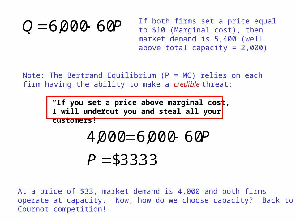
PQ 60000,6 If both firms set a price equal to $10 (Marginal cost), then market demand is 5,400 (well above total capacity = 2,000)
Note: The Bertrand Equilibrium (P = MC) relies on each firm having the ability to make a credible threat:
“If you set a price above marginal cost, I will undercut you and steal all your customers!”
33.33$
60000,6000,4
P
P
At a price of $33, market demand is 4,000 and both firms operate at capacity. Now, how do we choose capacity? Back to Cournot competition!
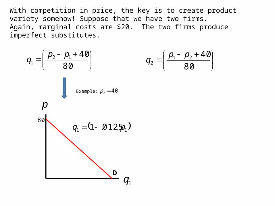
With competition in price, the key is to create product variety somehow! Suppose that we have two firms. Again, marginal costs are $20. The two firms produce imperfect substitutes.
80
40121
ppq
80
40212
ppq
1qD
80
p
402 p
11 0125.1 pq
Example:
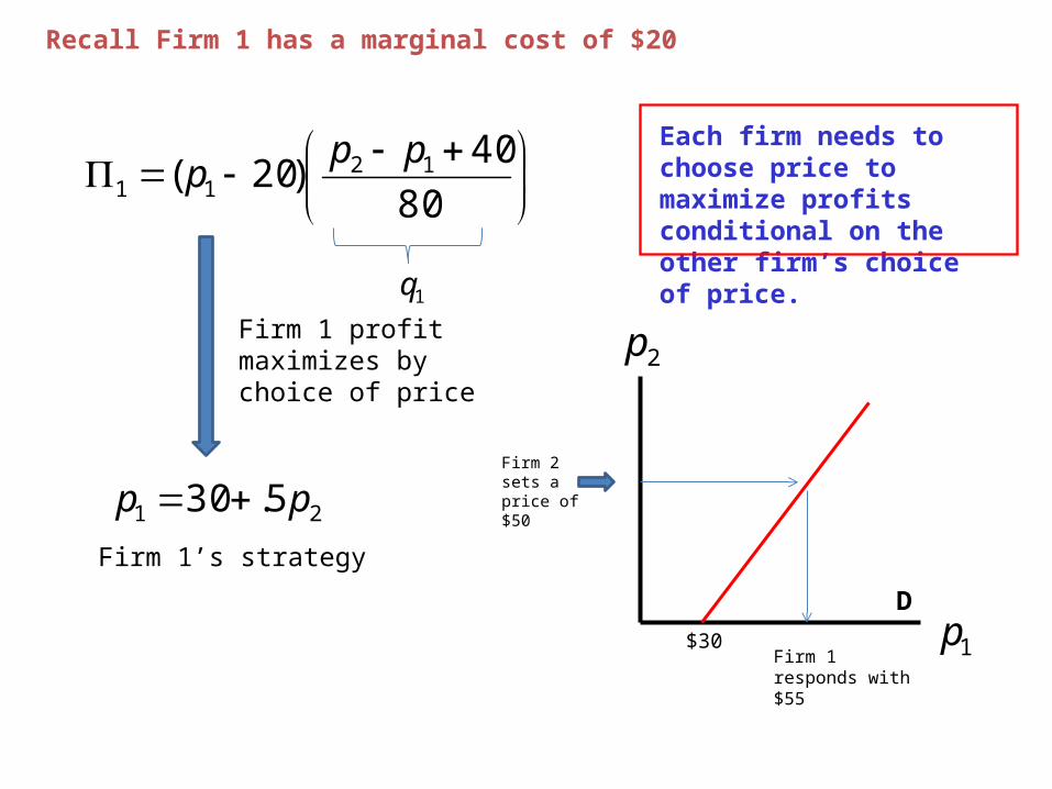
Recall Firm 1 has a marginal cost of $20
80
40)20( 12
11
ppp
Each firm needs to choose price to maximize profits conditional on the other firm’s choice of price.
21 5.30 pp
Firm 1 profit maximizes by choice of price
1pD
2p
Firm 1’s strategy
$30
Firm 2 sets a price of $50
Firm 1 responds with $55
1q
1p
2p
Firm 1
Firm 2
30$
30$
60$
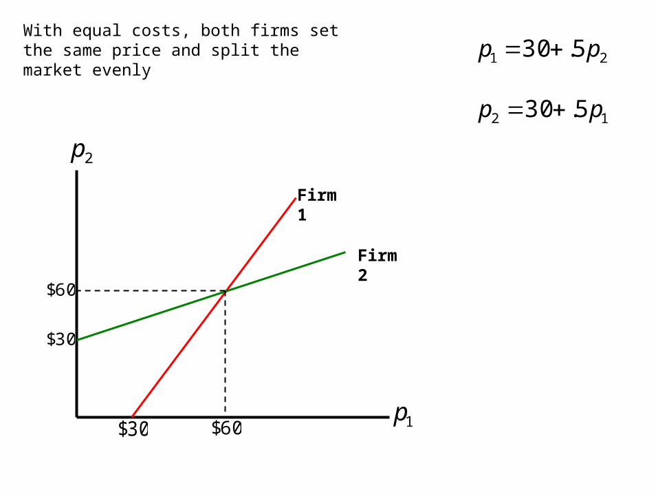
60$
With equal costs, both firms set the same price and split the market evenly 21 5.30 pp
12 5.30 pp
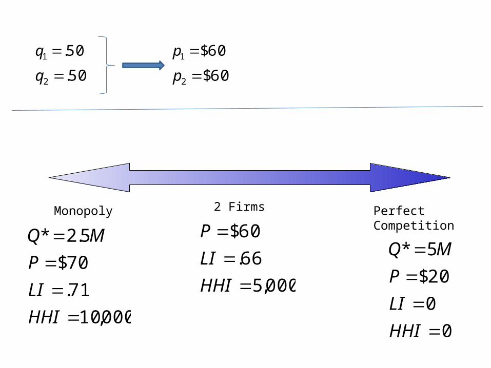
Monopoly
000,10
71.
70$
5.2*
HHI
LI
P
MQ
Perfect Competition
0
0
20$
5*
HHI
LI
P
MQ
2 Firms
000,5
66.
60$
HHI
LI
P
50.1 q
50.2 q
60$1 p
60$2 p
1p
2p
Firm 2
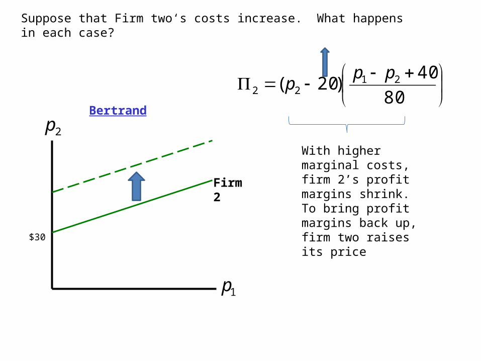
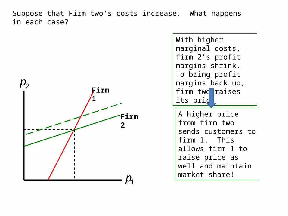
Suppose that Firm two‘s costs increase. What happens in each case?
Bertrand
$30
80
40)20( 21
22
ppp
With higher marginal costs, firm 2’s profit margins shrink. To bring profit margins back up, firm two raises its price
1p
2pFirm 1
Firm 2
Suppose that Firm two‘s costs increase. What happens in each case?
With higher marginal costs, firm 2’s profit margins shrink. To bring profit margins back up, firm two raises its price
A higher price from firm two sends customers to firm 1. This allows firm 1 to raise price as well and maintain market share!

Cournot (Quantity Competition): Competition is for market share
Firm One responds to firm 2’s cost increases by expanding production and increasing market share – prices are fairly stable and market shares fluctuate
Best response strategies are strategic substitutes
Bertrand (Price Competition): Competition is for profit margin
Firm One responds to firm 2’s cost increases by increasing price and maintaining market share – prices fluctuate and market shares are fairly stable.
Best response strategies are strategic complements
1p
2p Firm 1
Firm 2
1q
2q
Firm 1
Firm 2
Bertrand Cournot
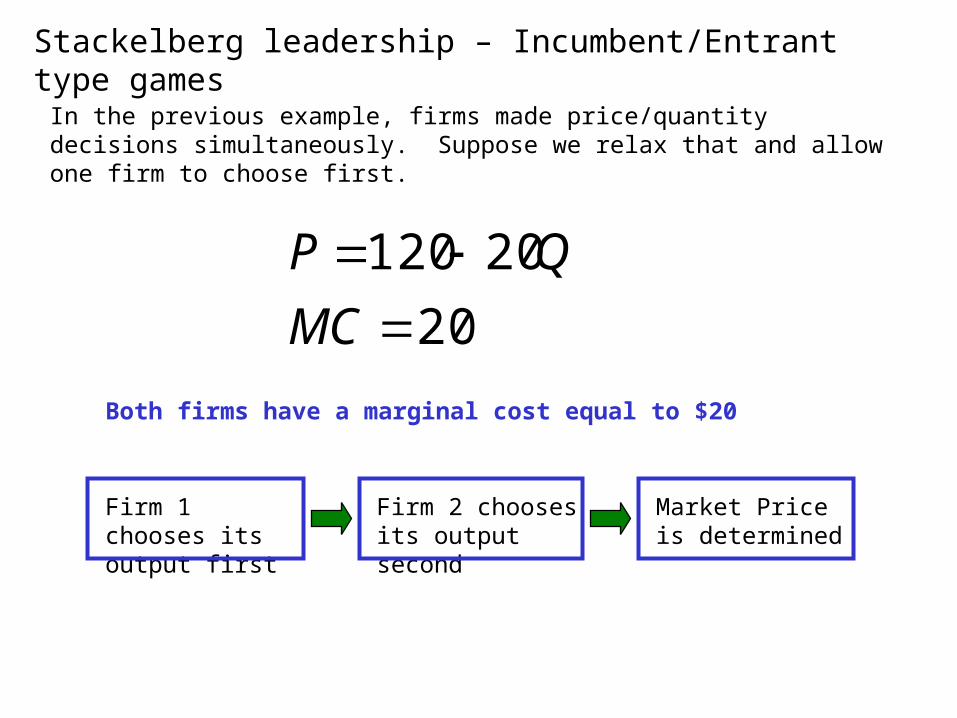
Stackelberg leadership – Incumbent/Entrant type games
In the previous example, firms made price/quantity decisions simultaneously. Suppose we relax that and allow one firm to choose first.
20
20120
MC
QP
Both firms have a marginal cost equal to $20
Firm 1 chooses its output first
Firm 2 chooses its output second
Market Price is determined
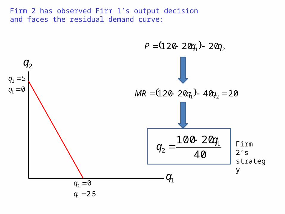
Firm 2 has observed Firm 1’s output decision and faces the residual demand curve:
21 2020120 qqP
40
20100 12
204020120 21 qqMR
1q
5.2
0
1
2
q
q
0
5
1
2
q
q
2q
Firm 2’s strategy
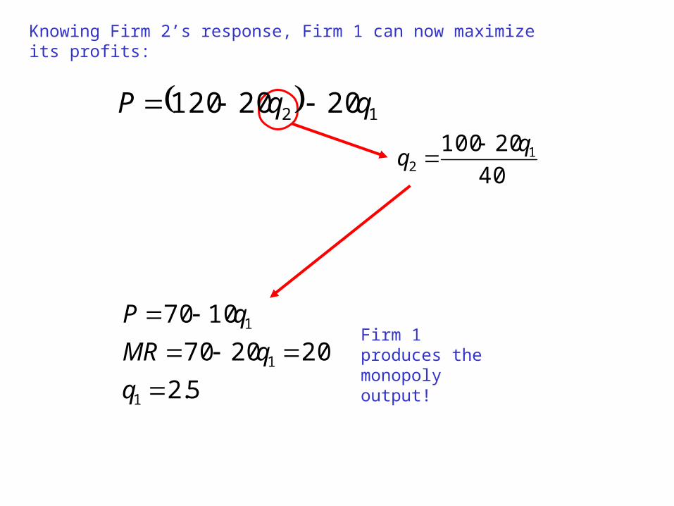
Knowing Firm 2’s response, Firm 1 can now maximize its profits:
12 2020120 qqP
5.2
202070
1070
1
1
1
q
qMR
qPFirm 1 produces the monopoly output!
40
20100 12
5.21 q 45$75.320120
75.3
P
Q
25.140
20100 12
25.3125.12025.145
50.625.2205.245
2
1
Monopoly
000,10
71.
70$
5.2*
HHI
LI
P
MQ
Perfect Competition
0
0
20$
5*
HHI
LI
P
MQ
2 Firms
587,5
55.
45$
25.1
5.2
75.3
2
1
HHI
LI
P
q
q
MQ(67%)
(33%)
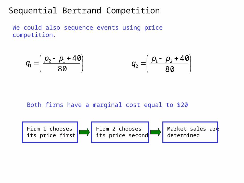
Sequential Bertrand Competition
We could also sequence events using price competition.
80
40121
ppq
80
40212
ppq
Both firms have a marginal cost equal to $20
Firm 1 chooses its price first
Firm 2 chooses its price second
Market sales are determined
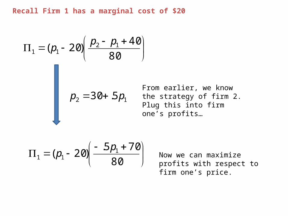
Recall Firm 1 has a marginal cost of $20
80
40)20( 12
11
ppp
12 5.30 pp From earlier, we know the strategy of firm 2. Plug this into firm one’s profits…
80
705.)20( 1
11
pp Now we can maximize profits
with respect to firm one’s price.
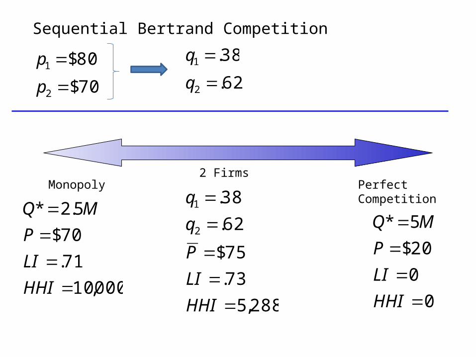
38.1 qSequential Bertrand Competition
80$1 p
70$2 p 62.2 q
Monopoly
000,10
71.
70$
5.2*
HHI
LI
P
MQ
Perfect Competition
0
0
20$
5*
HHI
LI
P
MQ
2 Firms
288,5
73.
75$
62.
38.
2
1
HHI
LI
P
q
q
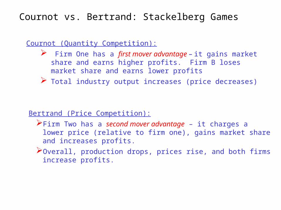
Cournot vs. Bertrand: Stackelberg Games
Cournot (Quantity Competition):
Firm One has a first mover advantage – it gains market share and earns higher profits. Firm B loses market share and earns lower profits
Total industry output increases (price decreases)
Bertrand (Price Competition):
Firm Two has a second mover advantage – it charges a lower price (relative to firm one), gains market share and increases profits.
Overall, production drops, prices rise, and both firms increase profits.
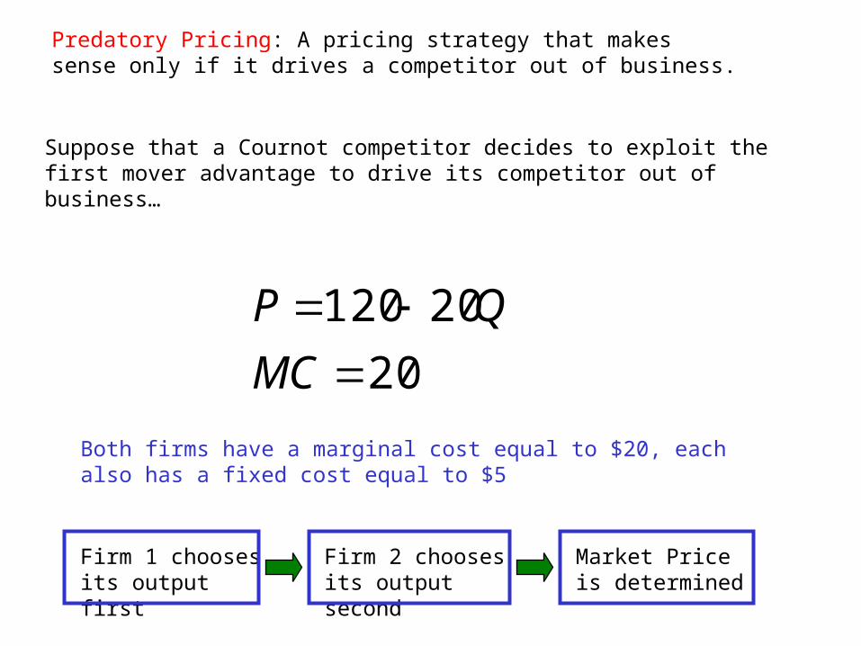
Suppose that a Cournot competitor decides to exploit the first mover advantage to drive its competitor out of business…
20
20120
MC
QP
Both firms have a marginal cost equal to $20, each also has a fixed cost equal to $5
Firm 1 chooses its output first
Firm 2 chooses its output second
Market Price is determined
Predatory Pricing: A pricing strategy that makes sense only if it drives a competitor out of business.
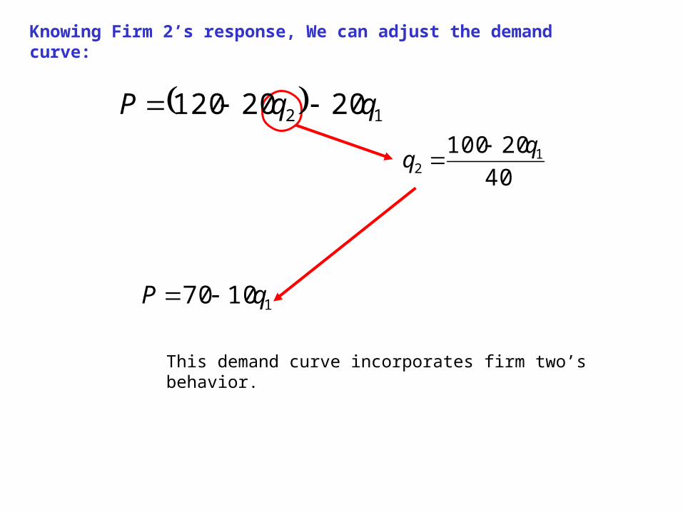
Knowing Firm 2’s response, We can adjust the demand curve:
12 2020120 qqP
11070 qP
40
20100 12
This demand curve incorporates firm two’s behavior.
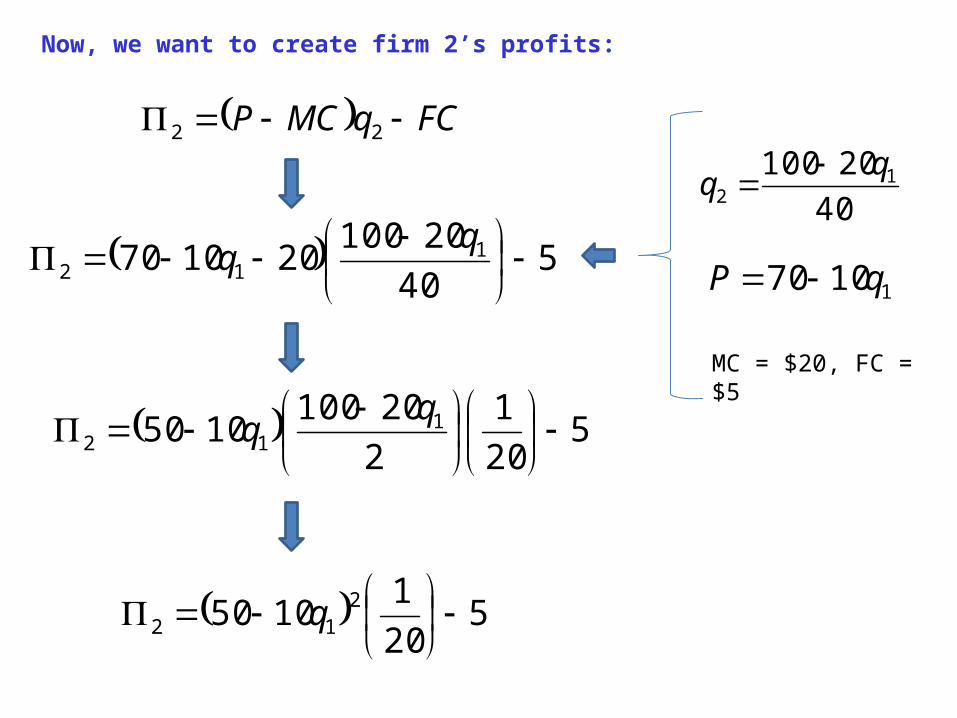
Now, we want to create firm 2’s profits:
11070 qP
40
20100 12
FCqMCP 22
MC = $20, FC = $5
540
20100201070 1
12
q
q
520
1
2
201001050 1
12
q
q
520
11050 2
12
q
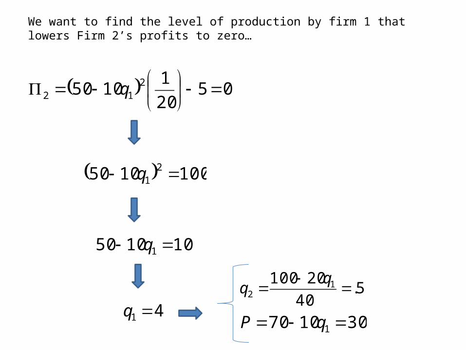
We want to find the level of production by firm 1 that lowers Firm 2’s profits to zero…
0520
11050 2
12
q
1001050 21 q
101050 1 q
41 q5.
40
20100 12
301070 1 qP
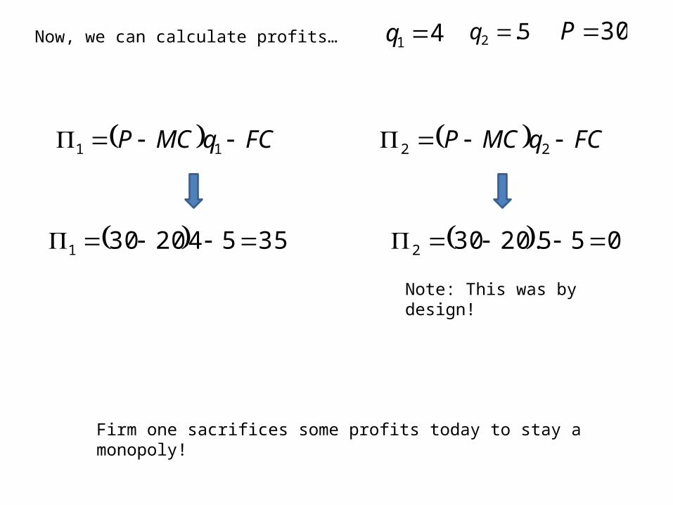
Now, we can calculate profits…
355420301
41 q 5.2 q 30P
FCqMCP 11 FCqMCP 22
055.20302
Note: This was by design!
Firm one sacrifices some profits today to stay a monopoly!
There have been numerous cases involving predatory pricing throughout history.
There are two good reasons why we would most likely not see predatory pricing in practice
1. It is difficult to make a credible threat (Remember the Chain Store Paradox)!
2. A merger is generally a dominant strategy!!
Standard Oil
American Sugar Refining Company
Mogul Steamship Company
Wall Mart
AT&T
Toyota
American Airlines
The Bottom Line with Predatory Pricing…
There have been numerous cases over the years alleging predatory pricing. However, from a practical standpoint we need to ask three questions:
1. Can predatory pricing be a rational strategy?
2. Can we distinguish predatory pricing from competitive pricing?
3. If we find evidence for predatory pricing, what do we do about it?