SANDIA REPORT SAND2011-5528 Unlimited Release Printed July 2011

Final Report: Testing and Evaluation for Solar Hot Water Reliability Dave Menicucci, Building Specialists Inc. Hongbo He, Andrea Mammoli, and Tom Caudell, University of New Mexico Jay Burch, National Renewable Energy Laboratory Prepared by Sandia National Laboratories Albuquerque, New Mexico 87185 and Livermore, California 94550 Sandia National Laboratories is a multi-program laboratory managed and operated by Sandia Corporation, a wholly owned subsidiary of Lockheed Martin Corporation, for the U.S. Department of Energy’s National Nuclear Security Administration under contract DE-AC04-94AL85000. Approved for public release; further dissemination unlimited.

2

Issued by Sandia National Laboratories, operated for the United States Department of Energy by Sandia Corporation. NOTICE: This report was prepared as an account of work sponsored by an agency of the United States Government. Neither the United States Government, nor any agency thereof, nor any of their employees, nor any of their contractors, subcontractors, or their employees, make any warranty, express or implied, or assume any legal liability or responsibility for the accuracy, completeness, or usefulness of any information, apparatus, product, or process disclosed, or represent that its use would not infringe privately owned rights. Reference herein to any specific commercial product, process, or service by trade name, trademark, manufacturer, or otherwise, does not necessarily constitute or imply its endorsement, recommendation, or favoring by the United States Government, any agency thereof, or any of their contractors or subcontractors. The views and opinions expressed herein do not necessarily state or reflect those of the United States Government, any agency thereof, or any of their contractors. Printed in the United States of America. This report has been reproduced directly from the best available copy. Available to DOE and DOE contractors from U.S. Department of Energy Office of Scientific and Technical Information P.O. Box 62 Oak Ridge, TN 37831 Telephone: (865) 576-8401 Facsimile: (865) 576-5728 E-Mail: reports@adonis.osti.gov Online ordering: http://www.osti.gov/bridge Available to the public from U.S. Department of Commerce National Technical Information Service 5285 Port Royal Rd. Springfield, VA 22161 Telephone: (800) 553-6847 Facsimile: (703) 605-6900 E-Mail: orders@ntis.fedworld.gov Online order: http://www.ntis.gov/help/ordermethods.asp?loc=7-4-0#online

3

SAND2011-5528 Unlimited Release Printed July 2011

Final Report: Testing and Evaluation for Solar Hot Water Reliability

David Menicucci

Building Specialists, Inc. 1521 San Carlos SW

Albuquerque, NM 87104

Hongo He, Andrea Mammoli, and Tom Caudell University of New Mexico Albuquerque, NM 87131

Jay Burch

National Renewable Energy Laboratory 1617 Cole Blvd.

Golden, CO 808401-3305

Sandia Purchase Order Nos. 95808 and 979664*

Abstract Solar hot water (SHW) systems are being installed by the thousands. Tax credits and utility rebate programs are spurring this burgeoning market. However, the reliability of these systems is virtually unknown. Recent work by Sandia National Laboratories (SNL) has shown that few data exist to quantify the mean time to failure of these systems. However, there is keen interest in developing new techniques to measure SHW reliability, particularly among utilities that use ratepayer money to pay the rebates. This document reports on an effort to develop and test new, simplified techniques to directly measure the state of health of fielded SHW systems. One approach was developed by the National Renewable Energy Laboratory (NREL) and is based on the idea that the performance of the solar storage tank can reliably indicate the operational status of the SHW systems. Another approach, developed by the University of New Mexico (UNM), uses adaptive resonance theory, a type of neural network, to detect and predict failures. This method uses the same sensors that are normally used to control the SHW system. The NREL method uses two additional temperature sensors on the solar tank. The theories, development, application, and testing of both methods are described in the report. Testing was performed on the SHW Reliability Testbed at UNM, a highly instrumented SHW system developed jointly by SNL and UNM. The two methods were tested against a number of simulated failures. The results show that both methods show promise for inclusion in conventional SHW controllers, giving them advanced capability in detecting and predicting component failures.

* This final report is issued jointly by BSI and UNM because the two purchase orders were inextricably linked.

UNM was tasked to provide testing capability and advanced research capability in support of BSI’s research and development activities regarding solar hot water reliability. The work described in this report was performed for SNL under Purchase Order No. 95808 (with BSI) and Purchase Order No. 979664 (with UNM).

4

5

TABLE OF CONTENTS

1. INTRODUCTION ......................................................................................................................9

2. BACKGROUND ......................................................................................................................10

3. EVOLUTION OF THE TESTING PROGRAM ......................................................................12 University of New Mexico Collaboration ................................................................................12 Literature Search ......................................................................................................................13 Sensors for Testing Reliability.................................................................................................13 Selection of Methodologies to Test .........................................................................................16 Selection of Methods for Testing .............................................................................................17 The Value of Predictive Failure Capability .............................................................................17 Theoretical Discussion About the Reliability Methods That Were Chosen for Testing .........18 Calorimetric Method Developed by Jay Burch..................................................................... 18 Adaptive Resonance Theory ................................................................................................. 19

4. TEST OBJECTIVES AND TEST PLAN .................................................................................21 Preparation for Testing ............................................................................................................21

5. TESTBED DEVELOPMENT ..................................................................................................23

6. PREPARING THE SHWRT FOR TESTING ..........................................................................31 Verification of the Accuracy of the Testbed Operation ...........................................................31

7. TESTING AND RESULTS ......................................................................................................36 Test Results From the Application of the ART Methods of Fault Detection to the Simulated Catastrophic Pump Failure .....................................................................................36 Detection of Failure Using the External TCs 4,5 .....................................................................38 Correspondence Between External Surface and Internal Immersed Temperature Sensors .....43 Results From Application of the ART Methods to Detect Impeller Degradation ...................44

8. CONCLUSIONS AND RECOMMENDATIONS ...................................................................47

REFERENCES ..............................................................................................................................50

Appendix A. Paper by Jay Burch, et al., Describing the Calorimetric Methodology .................51

Appendix B. Description of the Artificial Resonance Theory That Was Applied to Solar Hot Water Failure Analysis ............................................................................................................53

Appendix C. Adaptive Resonance Theory Code Used for Testing Solar Hot Water Failures ....59

Appendix D. Description of the Development and Verification of the TRNSYS Model Used in the Solar Hot Water Reliability Testbed Testing Program ..................................................71

Appendix E. Description of the Process for Using TRNSYS Model to Train the ART Algorithms ...............................................................................................................................85

Appendix F. Pictures of the Solar Hot Water Reliability Testbed at the University of New Mexico .....................................................................................................................................87

Appendix G. Functional Specifications for an Advanced Generation Solar Hot Water Controller .................................................................................................................................89

6

FIGURES

Figure 1. Pressurized loop system. ...............................................................................................24 Figure 2. Drainback system. .........................................................................................................24 Figure 3. Physical layout of the SHWRT. ....................................................................................25 Figure 4. Lennox LSC collector. ...................................................................................................26 Figure 5. Thermocouple trees. ......................................................................................................27 Figure 6. SHWRT instrumentation. ..............................................................................................27 Figure 7. Solar pump logic diagram. ............................................................................................29 Figure 8. LabView VI data sample. ..............................................................................................31 Figure 9. List of labels for channels of data..................................................................................31 Figure 10. Relationship of theta/theta0 versus time. .....................................................................34 Figure 11. Performance profile during test period. .......................................................................36 Figure 12. ART error detection during the test period..................................................................37 Figure 13. Closeup view of the ART error detection on the day of the fault. ..............................38 Figure 14. Location of external wall temperature sensors. ...........................................................39 Figure 15. Tank temperature data used in the analysis (the average of external TCs 4,5). ..........40 Figure 16. Measured versus predicted energy to tank. .................................................................41 Figure 17. Measured versus predicted Qto-tank, as a line plot. ....................................................42 Figure 18. Tank UA on three successive nights (fourth night did not pass the screens for

robustness). ..............................................................................................................................42 Figure 19. Start and stop times for the five days with solar data. Normal start/stop occurred

the first three days, and the pump never ran the last two days. ...............................................43 Figure 20. External and internal temperatures. .............................................................................44 Figure 21. ART system’s error reporting. .....................................................................................45

TABLES

Table 1. Traditional and Auxiliary Sensors. .................................................................................14 Table 2. State and Sensor Matrix for Systems With Traditional Sensors. ....................................15 Table 3. State and Sensor Matrix for Systems With Traditional and Auxiliary Sensors. .............16 Table 4. SHWRT Components. ....................................................................................................30 Table 5. Relationships between external and internal sensors. .....................................................44

7

ACRONYMS

ART Adoptive Resonance Theory ASHRAE American Society of Heating, Refrigerating, and Air Conditioning Engineers BSI Building Specialists, Inc. HECO Hawaiian Electric Company HVAC heating, ventilating, and air conditioning ME Mechanical Engineering NREL National Renewable Energy Laboratory PV photovoltaic SHW Solar Hot Water SHWRT Solar Hot Water Reliability Testbed SNL Sandia National Laboratory SRCC Solar Rating and Certification Corporation TC thermocouple UNM University of New Mexico VI (LabView) Virtual Instrument

8

9

1. INTRODUCTION

This document represents the final report for two contractual efforts that relate to testing and evaluation in support of research on solar hot water (SHW) reliability. Building Specialists Inc. (BSI) was tasked by Sandia National Laboratories (SNL) with developing a test and evaluation program with the intention of developing techniques for detecting and predicting faults in SHW systems (PO 955808). The University of New Mexico (UNM) was tasked by SNL with providing the test capabilities for the research effort along with advanced technological methods for detecting faults (PO 979664). This report represents the final deliverable for both efforts.

This report is organized in seven sections.

Section 2 provides background information, including the basic problem that has been investigated along with related prior work.

Section 3 describes how the testing program evolved.

Section 4 describes the test objectives and the test plan.

Section 5 describes the testbed development.

Section 6 discusses the work needed to prepare the testbed for testing, including a thorough review of the instrumentation system.

Section 7 presents the two sets of tests that were conducted, one of which was related to the neural network theory proposed by UNM and the other being a Calorimetric method theorized by Jay Burch at the National Renewable Energy Laboratory (NREL).

Section 8 presents the conclusions and recommendations.

The appendixes contain details to augment the summary information in the text.

10

2. BACKGROUND

This project is intended to more thoroughly understand SHW reliability. A major concern is that many SHW systems are being installed with the assumption that these systems will operate flawlessly for their expected lifetimes, typically 20 years. This assumption is almost certainly false because these systems typically contain a variety of mechanical components whose lifetimes are less than 20 years.

Many utilities are paying rebates to their customers who install these systems based on this contingency. In addition, utility planners, specifically the people who forecast electrical loads and design new generation and distribution systems, have an interest in understanding the reliability of SHW systems because if they fail, the utility must be prepared to supply energy to heat domestic water in their stead.

As more of these SHW systems are installed, the concern about SHW system reliability grows. Unfortunately, the actual lifetimes of SHW are not known with even a marginal level of certainty.

This project has a dual focus. The first is to achieve a more thorough understanding of the existing reliability data and the implications from these data. The second is to develop tools and techniques to help improve our ability to measure SHW system reliability and to improve the level of reliability in new systems.

In 2008, in discussions with technical staff from SNL, the research team1

The results were published in an SNL report [1] and the major finding from that investigation is that there is little consistency among the databases. In fact, in many ways the conclusions that can be drawn from one database tended to contradict the conclusions drawn from the others. In short, there were many more contradictions between the databases than similarities. Importantly, the best data that existed—a field survey of existing installations—indicated that 50% of the pumped SHW systems had failed during the first 10 years of their lifetime. Integral systems, which have no moving parts, fared much better, but even they had some unexpected failures.

agreed that the first logical effort would be to examine the existing reliability databases and compare them. Several databases had been assembled over the past 20 years but nobody had studied them for consistency. This was the focus of the 2008-2009 effort.

After that SNL report was released, Tim Merrigan (NREL) criticized it because it did not include the full set of data from the many systems that were installed in Hawaii, a project that was managed by the Hawaiian Electric Company (HECO) in the late 1990s and early 2000s. HECO representatives had presented summary data showing that the Hawaii systems were highly reliable. But during the first study HECO had been reluctant to release the data for inclusion in the analysis.

As a consequence, a second effort was initiated to collect and analyze any additional SHW reliability data that might exist. The goal was to ensure that all existing data were included in the SHW reliability database that was created in the 2008-2009 effort. A report on this effort has been drafted and is in the process of being published as an SNL report.

1 The research team consisted of Dave Menicucci, Greg Kolb and Tim Moss (SNL), and Tim Merrigan (NREL).

11

Another major issue was that there had never been a concerted effort to collect solar reliability data directly. All of the data that had been collected in the first study and the follow-on data study were based on opinions of installers, warranty records, or field surveys that were conducted a decade after systems were installed.

While valuable, these data did not contain the most pertinent information that would allow an accurate computation of the SHW system’s mean time to failure or system availability. Nearly all of the existing data about SHW systems pertained to their energy performance at the time of installation and during the period of warranty, typically a year or two into the systems’ life. Warranty-based databases rarely contain information about end-of-life system failures that typically occur many years after the warranty has expired.

A conclusion was that tools and techniques are needed to address this shortcoming and to develop data that could be analyzed with the intention of improving reliability. But there was no place to develop and test any new techniques or tools, even if any existed. Therefore, a test program was required, including the development of a testing platform where reliability issues could be studied in a controlled manner.

The SHW reliability improvement effort has two parts. The first part was intended to collect and analyze any additional SHW reliability data that might exist. The second was intended to develop a program that could be used to develop and test new ideas regarding various aspects of SHW reliability.

This document reports on the second part of the effort, the testing and evaluation that was conducted at UNM.

12

3. EVOLUTION OF THE TESTING PROGRAM

University of New Mexico Collaboration

One of the basic problems with SHW systems is that when failures occur in installed systems, there are few obvious negative consequences. In short, nothing of significance happens when a SHW system fails because the backup water heating system silently picks up the load. Unless system owners are regularly monitoring their systems, they will not notice when they are offline due to failures. Most SHW controllers have no capability to recognize a failure in the system or to notify the owner that a problem exists.

The research team agreed that some tools were needed to identify failures. There was also the belief that new products should be tested, such as advanced SHW controllers, that purported to identify failures in SHW systems. Thus, a testbed was needed for SHW reliability testing. A university is an excellent venue for such a testbed.

In attempting to develop the testbed project a number of labs and universities were contacted. UNM was the only one that responded with interest. In fact, Andrea Mammoli, of the Mechanical Engineering (ME) Department, responded enthusiastically and suggested that not only would UNM co-fund such a project, but that they would contribute novel and unique concepts and ideas for cutting edge technology that might offer unique capabilities for detecting and predicting faults in SHW systems. These capabilities would be provided for testing and evaluation on the testbed.

Mammoli and his team had been considering reliability of SHW systems, and when this opportunity arose they quickly seized the opportunity to collaborate. Mammoli proposed that one of his PhD candidates, Hongbo He, would apply Adaptive Resonance Theory (ART) to this problem. Fundamentally, ART is an artificial learning process that can be programmed on a computer. The algorithms that comprise ART can essentially be taught the equivalent of human intuition and can use that artificial intuition to identify and possibly predict failures. The UNM team had developed the theory, but had no platform to test it. Thus, the idea of creating a testbed at UNM was enthralling because, for the first time, the ART theory could be tested on a real SHW system, the best possible trial.

The UNM/BSI/SNL collaboration was an excellent one to achieve the testing objectives. First, the testbed would be located near SNL and BSI, thus eliminating expensive travel. Second, UNM offered to contribute resources to the project in terms of technology, along with labor to build the testbed and to operate it. Third, working collaboratively, UNM and BSI had some new ideas to apply to the reliability problem. ART was a concept that had never been applied in the SHW industry and seemed to be ideally suited for the reliability problems under consideration.

The testbed would consist of a fully instrumented SHW system that could be used to test various reliability concepts and tools (such as SHW control systems that are purported to have the capability to identify failures). Hongbo He would apply ART to the testbed as part of his doctoral thesis. Other students, including Jeremy Sment (senior undergrad) and Glenn Ballard (MS candidate), would assist in various facets of the project, such as developing the system controls, which had to be much more sophisticated than the simple controllers used in commercial systems. The testbed controller had to collect data and control failures, things that normal controllers do not do.

13

By early November 2009 a plan was developed. Sandia agreed to provide contract funding to UNM for hardware for a testbed that would be located at UNM’s ME Department. Andrea Mammoli (UNM) and Dave Menicucci (BSI) were the co-principal investigators in the effort.

Literature Search

The technical work began with a literature search. The UNM library was used to search for articles and other information about SHW reliability measurements/monitoring. Also, a number of organizations who are involved with SHW monitoring or manufacturing monitoring equipment were contacted to know what products might already exist and what capability they have relative to the question that was under investigation, especially reliability monitoring.

For clarity, the term “reliability monitoring” and like descriptors means that the SHW system is being monitored by a device with the capability to identify a system failure and take measures to manage the failure to prevent further damage. Such a monitoring system would also have the capability to sound a warning to the owner or operator of the system so that appropriate remedial action can be taken. An advanced reliability monitoring system might also have the capability to provide diagnostic information, such as identifying the potential failed or failing component.

Previous literature searches for SHW reliability monitoring equipment and ideas had produced little or no useful information. The more intensive search conducted in this project produced no new publications or other information.

The organizations that were contacted included the following: Goldline Controls, IMC Instruments, Heliodyne, Qisol, and Fat Spaniel. Many newer SHW controllers, such as IMC’s Eagle 2, are designed not only to control the SHW system but to monitor performance as well.

None of the current commercially available controller and/or energy products (Heliodyne, IMC, and Goldline) have more than cursory capability to perform reliability monitoring of SHW systems. Representatives of these companies all expressed some interest in the possibility of applying advanced reliability monitoring capabilities, if they could be proved accurate and useful.

The largest commercial renewable energy system monitoring organization, Fat Spaniel, focuses its monitoring services on energy production of photovoltaic (PV) systems but has interest in eventually providing monitoring services for solar thermal systems. At this time Fat Spaniel has no capability to conduct reliability monitoring.

Only Qisol had a product that was purported to contain the capability of reliability monitoring. At that time, about a year ago, the technology owner, David Collins, was interested in participating in experimental efforts to develop a deeper understanding about SHW reliability and indicated a willingness to supply a prototype version of his metering system for test on an experimental test platform. Unfortunately, he was unwilling to divulge technical details about how his metering system operates, even if these details were protected from disclosure with a nondisclosure agreement. Nonetheless, this appeared to be a positive possibility.

Sensors for Testing Reliability

The discussions with the manufacturers along with the literature search produced useful information, especially about the type of information that is needed to detect failures. By combining this information with common knowledge about the operational characteristics of

14

SHW systems, the research team created two matrices that described the various sensors and their operational characteristics in a system that is operating properly and one that has failed. The information in these matrices can be used to develop the required sensors and the array of tests that can be used to monitor a SHW system for reliability.

One matrix was based on the assumption that only the traditional sensors that are commonly available in commercial SHW systems would be available for monitoring. The other matrix contains those sensors that are listed in the first matrix plus other additional sensors that might be considered for future reliability monitoring equipment.

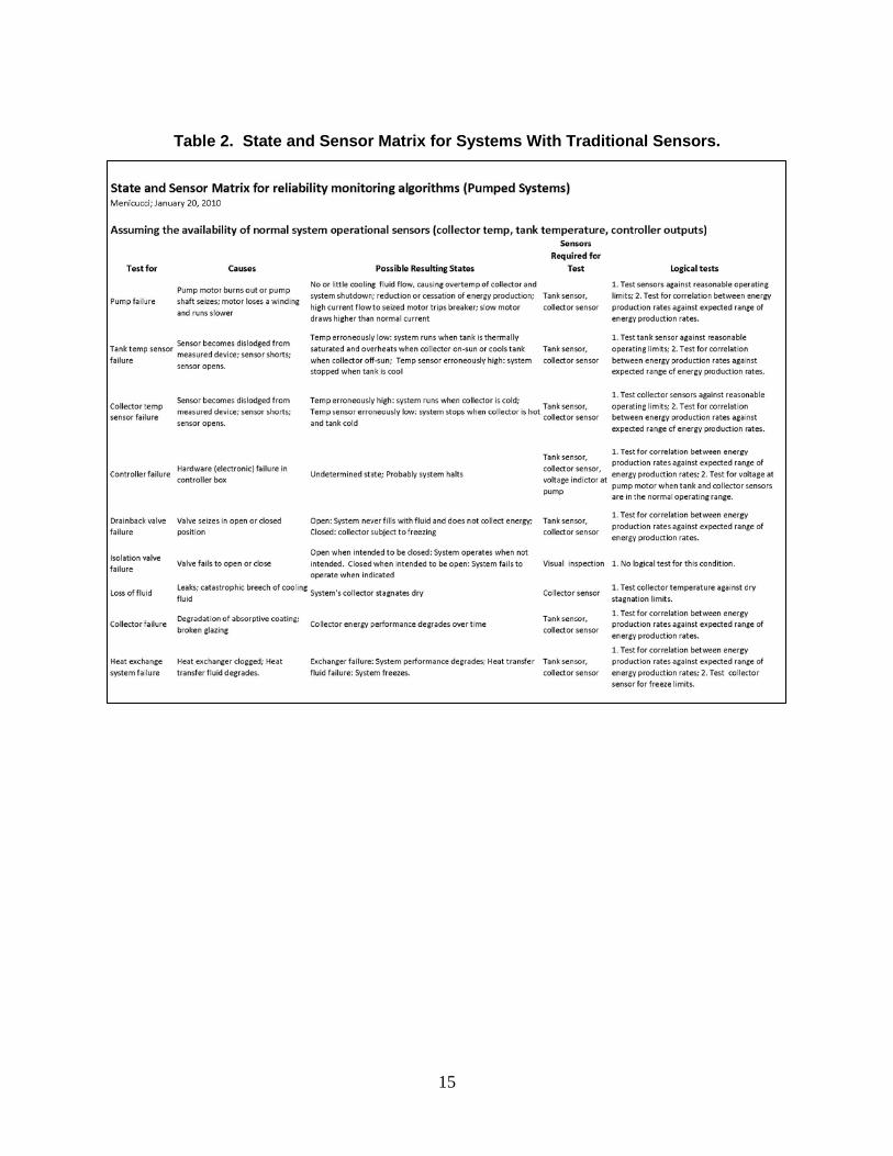
Table 1 lists the traditional sensors and auxiliary ones. The sensors’ functions are obvious by their name. These sensors were all candidates for inclusion in the SHW reliability testbed being developed at UNM.

Table 1. Traditional and Auxiliary Sensors.

The two matrixes are presented below. Table 2 pertains to systems that have only the commonly available sensors. Table 3 pertains to systems that have common sensors plus auxiliary ones.

Normal operational sensors Auxiliary Sensors

Tank temperature sensorCurrent CT sensor on pump motor

Voltage indicator sensor at pump motor

Insolation sensor

Collector temperature sensor

Flow meter, insolation sensor

Visual inspectionHX inlet and outlet temperature sensors

15

Table 2. State and Sensor Matrix for Systems With Traditional Sensors.

16

Table 3. State and Sensor Matrix for Systems With Traditional and Auxiliary Sensors.

The matrices contain a list of the various components involved in system operation and the sensors that would be involved in a test to determine if that particular component has failed or is in the process of failing (see column “Test for”). The column labeled “Causes” describes the possible failure states. The “Resulting States” are listed in the next column. The sensors involved in the test are listed in the next column(s). The last column, “Logical Tests,” describes the tests that would be applied to determine the state of the component.

Selection of Methodologies to Test

A number of solar controllers were identified for possible SHW reliability testing. These included the following: Goldline Controls, IMC Instruments, Heliodyne, Qisol, and Fat Spaniel.

Of these, only Qisol had a product, which at the time was in advanced stage of testing, to monitor SHW reliability. The owner, David Collins, was interested in participating in an experimental effort to develop a deeper understanding about SHW reliability and to supply a prototype version of his metering system for test on an experimental platform. However, Collins was unwilling to divulge details about how his metering system operates, information that is

17

needed to design an appropriate test plan. At a later time, after he finished his development, he was to have contacted the UNM/BSI team to arrange for testing. However, he never contacted the team and numerous email and telephone attempts to contact Collins through his company website were not successful.

Selection of Methods for Testing

Two new concepts for monitoring reliability remained in contention for inclusion in the testing program. The first is the tank calorimetric method developed by Jay Burch of NREL. The second is the ART work by Hongbo He and Professor Tom Caudell of UNM, Hongbo’s co-advisor (Andrea Mammoli was Hongbo’s principal advisor).

Both of methodologies held promise for creating algorithms that could be integrated into SHW system controllers in the future.

The methodology developed by Burch requires a sensor to be installed on the external skin of the storage tank of an SHW system. This sensor would be in addition to the sensors that are normally installed as part of traditional commercial controllers. However, this sensor is low cost and placing it on the middle portion of the tank is possible without extraordinary effort. Therefore, the cost for this addition is reasonably low and the benefit would be that the controller would have greatly enhanced capabilities to monitor the health of the solar system during operation.

The ART methodology, described above, holds equally high potential for application in SHW controllers. This methodology, while more complex than Burch’s method, holds the promise of not only being able to identify a failure of a component, but possibly being able to predict the failure of a component. Most important, the method does not need any additional sensors from what is normally required by a commercial controller to operate the SHW system.

Further, both Burch’s technique and the ART operate on the principle of a computerized system that can artificially learn patterns of typical system behavior and then be able to recognize when these patterns have abnormally changed. The ART method learns in a manner similar to that used by living creatures. The Burch technique depends on the hysteresis that is inherent in a SHW system’s storage tank in which its temperature conditions represent a record of system’s past performance.

The ART directly applies advance neural network methodologies that are extremely robust and capable in this task. What is more, these techniques are not static. When applied in a real system, the ART’s learning process continually gleans more about how the system operates, just as a human operator might do. Thus, it effectively becomes more intelligent over time and becomes more adept at recognizing abnormalities and differentiating them from normal variance in operation due to factors such as changing temperatures, insolation, and loads.

Based on this rationale, the Burch and the ART methods were selected for testing.

The Value of Predictive Failure Capability

The reliability of an SHW system can be tremendously improved by replacing components before they fail instead of replacing them as they fail. The reason is that after the burn-in period,

18

the initial operation time where early failures appear, the constant failure rate2

However, as the system approaches a time when critical components are reaching the end of their lives, the failure rate dramatically increases. The probability of a failure in this part of the lifetime of a system is predicted using the Gaussian distribution, which includes a mean and a standard deviation of the time to the end of life. As components age beyond the mean lifetime, the probability of failure increases and so do their failure rates.

is determined by chance occurrences, and the reliability of the system at any time during the life of the system after burn-in and before its end of life approaches is predicted by the exponential function. Bazovsky [2] provides a more complete discussion of the mathematical model for reliability and the use of the exponential function for devices and systems. The failure rate during that operational time period is low. Thus the mean time between failures is very long because the mean time between failures is equal to the reciprocal of the failure rate.

The key to a very high probability that the system will remain in a functional state is to replace the critical devices as they approach their end of life, at a point when their failure rate is approximately equal to the failure rate during the middle portion of their life, the time where reliability is controlled by chance failures. This replacement point is relatively easy to compute, if a mean and standard deviation are known for the lives of the components in question.

Unfortunately, these critical mean and standard deviation parameters are virtually unknown for SHW systems. Even with all the data that that have been collected, sorted, organized, evaluated, and studied in a previous effort conducted last year, none of these critical measures can be computed or estimated with certainty. Thus, at the present time and until sufficient data are collected specially to measure the critical items, there is no way to select the right time to replace components in an SHW system. Even starting today, collecting the required data would require many years before sufficient information existed to meet the needs of the statistical techniques.

In the absence of good quality statistical data that would identify a specific time to preemptively replace components, this leaves as a tool only those techniques that can identify an impending failure of a component in time to allow it to be replaced when the system is normally down, such as at night or when the sun is obscured. In this environment, the ability to predict a failure is extremely valuable.

Theoretical Discussion About the Reliability Methods That Were Chosen for Testing

Calorimetric Method Developed by Jay Burch Jay Burch et al., of NREL [3], have conceived of a rudimentary method of data collection over time in which a history of an SHW’s tank temperature fluctuations are recorded and characterized. This historical temperature profile is compared with the predictions based upon the collector, piping, heat exchanger, and tank characteristics. A simple theoretical model of performance is established, and serves as the reference for the actual tank temperature fluctuations. If solar radiation is not measured (as would be the usual situation), the model uses the American Society of Heating, Refrigerating, and Air Conditioning Engineers (ASHRAE) 2 The failure rate is usually expressed as a number of failures per unit time. Typically this failure rate varies over

the life of mechanical systems with higher failures during the startup and end-of-life phases and lower rates during the middle portion of the lifetime, sometimes called the useful or productive life period. During a system’s useful life period the failure rate is usually constant.

19

clear-sky algorithms for solar incidence. If the SHW fails or begins to fail, the temperature profile of the storage tank will be significantly different from the clear-day assumption. Without solar radiation data, it is only with statistical probability that a failure is detected, because there is always some probability of a sequence of totally cloudy weather.

The methodology has been published in two papers. The latest one is included in Appendix A, reproduced with written permission from the author [3].

The principal questions to be answered in the application of the Calorimetric method to SHW systems is whether the method can be successfully applied to identify and predict failures and to determine the number of sensors required to do so.

Adaptive Resonance Theory The UNM ME Department, in collaboration with Professor Tom Caudell in the Electrical and Computer Engineering Department, are developing some concepts for using neural networks to develop an advanced reliability monitoring scheme for solar thermal systems. Specifically, networks based on ART and its derivatives were used in this work [4].

Fundamentally, a neural network mimics a human brain with the principal characteristic being its ability to artificially learn and self-organize over time, and then to make intelligent decisions in the future based on the learned information.

Learning systems in neural networks can either be supervised or unsupervised. In supervised learning, statistical procedures are used to develop mathematical functions that fit groups of dependent and associated independent variables. Regression analysis is an example of a kind of supervised learning.

Unsupervised learning is geared to identifying the best type of function to represent a group of dependent and independent variables using optimization techniques. It is the kind of learning continuously employed by humans and other animals in their lives and results in what is often referred to as intuition.

The ART class of neural networks fits in the category of an unsupervised learning system. It is particularly well-suited to the task of performance monitoring and fault detection of an SHW system, because these can artificially learn and categorize vast amounts of data efficiently. They can be used to effectively recognize new input patterns in a stream of data that do not fit into any existing category [5,6].

The ART network algorithms must be trained in order for them to be applied. This “training” is equivalent to the process of human education and on-the-job training. To train the algorithms, data about the operation of a system must be recorded and then provided to the ART algorithms, essentially representing what humans would call “experience.” In the case of an SHW system, these experiential data might include the temperatures in the solar loop and solar tank. If these data represent normal operating conditions, then the ART algorithms artificially learn normalcy for that system. The more training that is done, the more artificially intelligent the algorithms become, especially in their ability to understand that variations in the performance of the system is a normal part of operation (e.g., an SHW system’s performance varies as a function of sunny weather, night-time, cloudy weather, etc.).

Analogously, this training is similar to the training that a human power plant operator might receive based on his or her experience in watching the plant operate over time. The operator

20

begins to understand the functional characteristics of the plant along with the vagaries of the plant’s normal operation.

Once the fundamental training is complete, then the algorithms are set to detect faults. Basically a fault is a condition that is outside the domain of what was previously experienced during the training. Thus, when this fault condition occurs, the unique nature of the conditions is immediately flagged by the algorithms as being outside of its experiential base. Additionally, the algorithms should also be able to detect degradation, as might be associated with a failing component. This predictive capability is most valuable for intermittent generators, such as SHW, because it would allow a repair before a catastrophic failure and at a time when the generator is not normally operating.

It is important to note that predicting failures in systems is not new. In the airline industry, for example, components in airplanes are routinely replaced before they fail. But these replacements are based on very well-defined statistical measures that have been computed from a long history of actual experience. The distinguishing characteristic of ART technology is that while it uses historical information for its training (based on actual experience or modeled experience), it develops artificial intuition about the system over time, essentially mimicking that of a human. This implies that ART can become more useful in predicting failures on systems that have a limited operational history and that its capabilities will become more robust over time.

Self-learning will occur based on false-positive indicators, the condition where the ART system has erred in identifying a fault. Once the human operator indicates that the fault condition was part of the normal behavior for the system, that event is integrated into the experience base of the algorithms, and if it were to recur it will not again be flagged.

Using this approach, a neural network learns over time the operational characteristics of an SHW system. Certain relationships among sensors can be established relative to environmental and load conditions. If a component begins to fail and its performance signature changes, other aspects of the system will be affected and at some point will be sufficiently noticeable to be acted upon. This condition would produce either a warning that a component is in the process of failing or has catastrophically failed.

The principal questions to be answered in the application of ART to SHW systems is whether the unsupervised learning mode can be successfully applied to identify and predict failures on a complex physical entity, such as an SHW system. Another goal is to determine the quantity and frequency of data needed to produce a measure of intuition in the control system that is sufficient to predict and/or identify failures. Fundamentally, a goal is to optimize the number of sensors, the frequency of data retrieval, and the history of measurement for maximum development of an artificially intelligent reliability monitoring system.

The theoretical basis for the ART technology is explained in more detail in Appendix B. Appendix C contains a copy of the ART code.

21

4. TEST OBJECTIVES AND TEST PLAN

This testing program was intended to answer the most fundamental questions about the ability of NREL’s Calorimetric technique and UNM’s ART methods to identify and predict failures.

A test plan was developed that included two major tests. The first test would simulate a catastrophic failure of the circulating pump on the solar loop. In this test the pump would suddenly be turned off, just as would happen if a pump motor burned out.

A second test would simulate the degradation of the pump’s impeller as would occur in the case that debris is in the solar loop, such as balls of solder that were introduced into the piping when joints were over-soldered. In this case the impeller blades would be slowly peened over time, resulting in diminishing ability to move water in the pipe and characterized by reduced flow rates over time.

Data recorded from the tests, which include the full array of parameters that are recorded by the Solar Hot Water Reliability Testbed (SHWRT), would be supplied to Jay Burch and Hongbo He for analysis. Subsequently, each researcher would apply his respective reliability methodology to determine whether the failures can be detected.

In the first test the SHWRT would be operated in a normal mode for several days to let the system operation stabilize, especially the tank temperature.3

The plan for the second test was similar to test one, but the failure would not be catastrophic. Instead, the flow rate in the solar loop was to be reduced slowly over a period of four days (about 10% per day) with the fifth day returning the flow to normal. A circuit setter on the solar loop allowed the flow rate to be adjusted manually.

Four days of operation were planned for stabilization. On the fifth day, a catastrophic pump failure would be introduced on the solar loop by disabling the pump motor during normal operation. The test period was to be planned for a time when the weather conditions were to be generally clear for the entire duration of the test, although small amounts of intermittent cloudiness would be tolerated.

Preparation for Testing

The NREL methodology was essentially ready to be applied as soon as the tests were completed. However, this method required thermocouples to be installed on the skin of the solar storage tank (located on the metal tank between the exterior insulation and exterior face of the water-bearing metal tank). Details about the thermocouples can be found in Sections 5 and 6.

The ART system required substantial preparation. First, the ART algorithms had to be trained. Training is the artificial learning process where the adaptive resonance algorithms come to recognize normal operations. As was noted above, the longer the training period, the more sensitive the ART system will be in differentiating failures from normal operations.

In the optimal case training is done by monitoring a real system, the same one in which the ART system will be applied. Preferably, many years of training are expected to provide the best results, with each subsequent year producing better results than the previous one.

3 Normal operation means that the testbed is operating the SHW system in the same mode as a typical one, which

includes an active solar loop and electric backup heating in the storage tank.

22

In this case, the time frame for the test was much shorter that the optimal time required for training because and no fully operating system was available (the SHWRT operates for testing, and does not operate on a production basis).

To accomplish the training, a computerized system model of the SHWRT was developed and verified. This model was used to provide the data needed for training by running it with a standard Solar Rating and Certification Corporation (SRCC) load profile and five years of SOLMET data for Albuquerque. SOLMET data are hourly weather records for a 30-year period. The output from the model, an hourly record of SHW system performance, was then used to train the ART algorithms, effectively substituting for training on a real system. Appendixes D and E contain detailed information about how the TRNSYS model was verified and how the ART algorithms were trained.4

4 The use of the word “algorithm” here is based on a broad interpretation of its traditional meaning, which

typically refers to a piece of computer line code which remains fixed unless deliberately modified by a human.. In this case, however, this code learns and self-organizes, distinguishing it from the conventional connotative meaning of the word “algorithm.”

23

5. TESTBED DEVELOPMENT

Concurrent with the preparatory work described in Section 4, the testbed was developed. The technical team was ready to proceed by early 2010. Unfortunately many delays ensued due to procurement difficulties at both SNL and UNM. The contract was finally placed with UNM and money was available for the project by mid-spring 2010.

Furthermore, additional delays were incurred as the BSI and UNM personnel struggled to organize themselves into an efficient work team. Although BSI brought experience in building homes, this was an experimental project and construction could not move with the speed of a home project.

An important point is that unlike SNL where there are skilled technicians with a plentiful supply of tools for a project like this, UNM had limited tools and few on-site tradespeople and technicians that could be called upon for assistance. Thus, the principal investigators had to supply personal tools and direct labor to construct the testbed.

Also, Mammoli, co-principal investigator, is a full-time professor in the ME Department. He was heavily laden with the ordinary tasks of a full-time teaching professor and could not spend significant time on the project. Typically only about a day a week (+/-) could be dedicated to the construction. Occasionally, Mammoli was absent for extended periods to conduct other essential UNM business that was off site. Since many design modifications were required during construction and because the project was being conducted on school property, it was not appropriate to move forward with less than the complete team.

Additionally, the control system was much more complex than was originally anticipated. LabView was selected as the controlling interface because it was best suited to meet the technical requirements. But the team had limited familiarity with it. Mammoli originally assigned a senior undergraduate the task to build the controller, but the problem was too complex for him. BSI became intimately involved with the project, learning LabView, developing logic diagrams, and helping the student along. However, the complexity soon overran the combined expertise of those two individuals.

There were other problems and associated delays, but by end of spring 2010 the project was well behind schedule. At that point BSI embedded itself into the UNM team, securing an office, phone, and parking space, and coming into the office on a regular basis. The purpose was to supplement the labor and expertise needed to move the project along.

The labor expended by UNM and BSI on the project was far greater that had been planned, perhaps by an order of magnitude. The effort included many full days of work on weekends and some late evenings. But as progress became apparent, the entire team was invigorated as the world’s first and only solar reliability testbed began to emerge.

Due to the delays both contracts were extended in August at no cost.

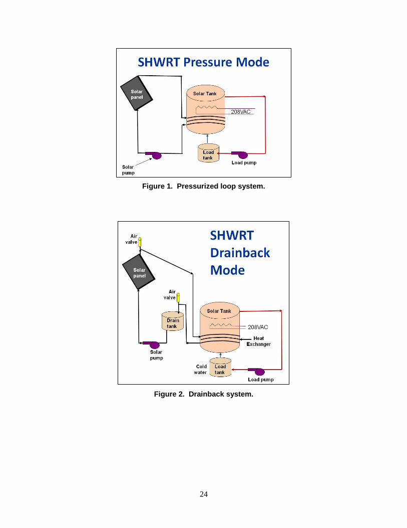
The testbed hardware was completed in October 2010. As was planned, it had the capability of being configured to represent two kinds of SHW systems, a pressurized loop system (see Figure 1) and a drainback system (see Figure 2). These are the most popular types of active SHW systems. Figures 1 and 2 show the two system configurations for the SHWRT. Figure 3 shows the physical layout of the system.

24

Figure 1. Pressurized loop system.

Figure 2. Drainback system.

25

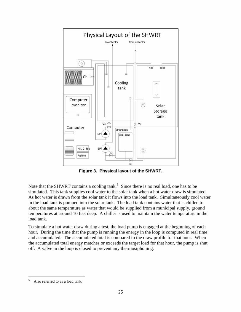
Figure 3. Physical layout of the SHWRT.

Note that the SHWRT contains a cooling tank.5

To simulate a hot water draw during a test, the load pump is engaged at the beginning of each hour. During the time that the pump is running the energy in the loop is computed in real time and accumulated. The accumulated total is compared to the draw profile for that hour. When the accumulated total energy matches or exceeds the target load for that hour, the pump is shut off. A valve in the loop is closed to prevent any thermosiphoning.

Since there is no real load, one has to be simulated. This tank supplies cool water to the solar tank when a hot water draw is simulated. As hot water is drawn from the solar tank it flows into the load tank. Simultaneously cool water in the load tank is pumped into the solar tank. The load tank contains water that is chilled to about the same temperature as water that would be supplied from a municipal supply, ground temperatures at around 10 feet deep. A chiller is used to maintain the water temperature in the load tank.

5 Also referred to as a load tank.

26

The SHWRT system employs two Lennox LSC-18 collectors, each with low-iron double glazing and black chrome absorber, as shown in Figure 4.6

The collector was manufactured in the early 1980s and was SRCC OG100 rated. Until it was installed in the SHWRT it had been stored in the basement of UNM’s ME Building.

Figure 4. Lennox LSC collector.

The SHWRT is a testbed and as such it is much more highly instrumented than a commercial system. For example, in a commercial SHW system there are normally two temperature sensors. One is located on the outlet of the collector and the other is on the supply line, at the outlet of the solar storage tank. The temperature difference between these two sensors is used by a commercial controller to turn on and off the solar loop pump. The SHWRT, however, contains many more sensors.

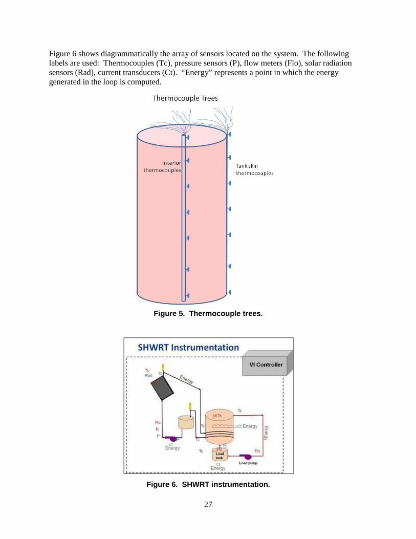
The solar tank and the load tank were outfitted with type T thermocouples. A thermocouple tree consisting of eight thermocouples was located along a plastic pipe that was installed in approximately the center of the tank. The plastic pipe was used only to hold each thermocouple in place, approximately equidistant from one another along the vertical axis of the tank.

Similarly, thermocouples were placed along the outside skin of the metal tank under the insulation in approximately the same vertical locations as those on the internal tree. To install them the exterior skin of the tank was carefully cut and the insulation was removed. The exterior metal surface of the water-bearing tank was cleaned and the thermocouples were glued in place using thermal epoxy.

Figure 5 shows graphically how the thermocouple trees are installed in the solar tank.

NREL supplied Agilent hardware to allow the SHWRT VI to incorporate additional thermocouples in the system.

6 Operation maintenance and installation instructions. Technical Report LSC18-1 and LSC18-1S Solar Collectors,

Lennox Industries Inc., July 1977.

27

Figure 6 shows diagrammatically the array of sensors located on the system. The following labels are used: Thermocouples (Tc), pressure sensors (P), flow meters (Flo), solar radiation sensors (Rad), current transducers (Ct). “Energy” represents a point in which the energy generated in the loop is computed.

Figure 5. Thermocouple trees.

Figure 6. SHWRT instrumentation.

28

All of the instruments were carefully calibrated before they were installed, and were tested again after they were installed. For example, the thermocouples were calibrated before installation. After installation they were again tested for consistency. More information about the calibration and tests can be found in Section 6.

After the hardware was built and tested, attention focused on the control system. The complexity of the LabView Virtual Instrument (VI) controller had been becoming apparent over the previous month, but it was not until the hardware was working that serious difficulties began to emerge. The complexity of this controller was much greater than would be found on a commercial SHW controller because the SHWRT system contained many more features than a commercial system, as discussed above. Additionally, the controller had to perform complex calculations during system operation to ensure that the various systems were all operating within safety limits, and that the data were written to a file.

As an example of this complexity, Figure 7 is the logic diagram for controlling the solar pump. Only a small portion of this logic would be implemented in a commercial controller.

Eventually, the team decided that additional professional help was required to complete the VI. SNL supplied Mike Edgar, a technician from SNL’s National Solar Thermal Test Facility, to provide assistance. Using the VI’s design specifications that the BSI/UNM team had created and working hand-in-hand with team members, he provided the necessary expertise to build the VI. By late December 2010 the VI was fully functional and was being tested for accuracy.

A summary of the components used in the SHWRT is summarized in Table 4.

29

Figure 7. Solar pump logic diagram.

30

Table 4. SHWRT Components.

Component Part Specification Collectors Lennox LSC-18 Storage Tank SunEarth SU80-HE-1 (nominal 80 gal, actual 73 gal)

,,,,,,,;asodhjffeiejsdngalactualnactualgal73gal72gal) Load Tank 55-gal. drum; insulated Load Tank Chiller Neslab RTE-8 Pumps B&G Plumbing Copper, Type L and M Instrumentation (pressure, flow, etc)

Mostly Omega

Thermocouple (TC) acquisition

Agilent 34970A

TCs Type K, Type T,welded in-house Instrumentation controller National Instruments Electrical device controller Custom designed and built with solid state relays

Pictures of the SHWRT hardware are found in Appendix F.

31

6. PREPARING THE SHWRT FOR TESTING

Verification of the Accuracy of the Testbed Operation

After the testbed was declared to be operational, the next step was to verify the accuracy of the many sensors in the system. Figure 8 shows a sample of the data that are recorded by the testbed’s LabView controlling VI. The first nine rows contain information about the manual settings for the test configuration. Such information includes, for example, the specific heat of the fluid in the loop (row one). Each column represents the data that was recorded at a specific time; the time is represented by a date and time in columns one and two. In the graphic below only 15 columns are shown.

Figure 8. LabView VI data sample.

Fifty-eight columns of data comprise each record. The complete list is noted in Figure 9.

Figure 9. List of labels for channels of data.

Sp. Heat Solar Loop (Eng.) = 0.895000Loop Stab. Time = 45.000000Max Header Temp = 105.000000Turn On Diff: Fin-S. Tank Ref. = 7.000000Turn Off Diff: Fin-S. Tank Ref. = 2.000000Max S. Tank Ref Temp = 55.000000Solar Pump Enable Diff = 2.000000Min Solar Tank Temp = 10.000000TC Sample Rate, s = 5.000000

Date Time

Room Ambient C

Outside Ambient C

Plane of array rad kW/m^2 Ref Cell

Outside Fin C

Collector Header C

To Solar Collector C

From Solar Collector C

Solar Pump Flow g/m

Pressure L

Pressure H

Solar Tank Top 120 C

Solar Tank 113 C

2/24/2011 11:24:09 26.667 13.363 1.101 0.178 63.997 56.293 53.387 55.435 1.938 14.985 29.134 47.323 48.1682/24/2011 11:24:39 26.723 13.684 1.096 0.179 64.028 56.322 53.423 55.459 1.93 15.12 29.144 47.39 48.182/24/2011 11:25:09 26.686 13.756 1.097 0.178 64.132 56.353 53.47 55.499 1.973 15.075 29.101 47.452 48.1822/24/2011 11:25:39 26.662 13.386 1.092 0.178 64.194 56.372 53.497 55.528 1.934 15.124 29.004 47.476 48.1872/24/2011 11:26:14 26.65 13.068 1.09 0.177 64.305 56.444 53.627 55.622 1.945 15.069 29.055 47.492 47.9552/24/2011 11:26:44 26.465 13.259 1.093 0.176 64.373 56.493 53.622 55.666 1.954 15.056 29.092 47.562 48.162/24/2011 11:27:14 26.233 13.313 1.093 0.174 64.295 56.557 53.618 55.68 1.956 15.015 29.024 47.545 48.2252/24/2011 11:27:49 26.201 13.913 1.09 0.18 64.25 56.541 53.634 55.73 1.948 15.03 28.934 47.48 48.227

Date Solar Tank 114 C Cooling Tank Mid C Disable TestTime Solar Tank 115 C Cooling Tank Bot C Low Temp FailRoom Ambient C Solar Tank 116 C Cooler In C Test AOutside Ambient C Solar Tank 117 C Cooler Out C Test BPlane of array rad kW/m^2 Solar Tank 118 C Cooler Flow Test C-1Ref Cell Solar Tank Bot 119 C Cooler Watts Test D-1Outside Fin C Solar Tank Ext-1 Target Hourly Load Wh Test C-2Collector Header C Solar Tank Ext-2 Load Accumulated Watt-hours Test D-2To Solar Collector C Solar Tank Ext-3 Heater Watts Test EFrom Solar Collector C Solar Tank Ext-4 Solar Pump Watts Heat SwitchSolar Pump Flow g/m Solar Tank Ext-5 Cumulative Solar Loop Wh Load Pump SwitchPressure L Solar Tank Ext-6 Cumulative Heater Wh Solar Pump SwitchPressure H Solar Tank Ext-7 Cumulative Load Wh Cooling SwitchSolar Tank Top 120 C Solar Tank Ext-8 FaultSolar Tank 113 C Cooling Tank Top C Logic Control

List of Labels for Channels of Data Recorded From the Testbed

32

Numerous tests on the individual sensors were conducted to ensure accurate data. For example, there are two pressure sensors in the solar loop. One is before the pump and one after the pump. When the system is not operating, both sensors should show readings that are approximately the equal. When the system is operating, the sensor downstream of the pump should read a higher value then the one upstream of the pump. The actual numbers were compared with rough hand calculations.

All of the flow meters were calibrated by hand, using a calibrated bucket and a stop watch. The accuracy of the SHWRT system was within 2.5% of the hand methods.

As described above, all the thermocouples were calibrated before they were installed and were re-examined after installation to ensure that they were not damaged during placement.

All of the thermocouples on the tree and along the skin were calibrated as groups against a mercury lab thermometer. The thermocouples on the internal tree were tested at low temperatures using an ice bath and found to be accurate to about 0.5 °C of the mercury thermometer. The thermocouples on the skin were compared to the mercury thermometer at the high end using a hot water bath and at the low end using an ice bath. All of these thermocouples were found to be accurate to within about 0.5 °C of the mercury thermometer.

After installation the thermocouples were re-examined. For example, the tank was partially heated and then allowed to cool. If all of the thermocouples are operating properly, they should record stratification in the tank with the hottest water near the top and the coldest at the bottom. The thermocouples on the skin should exhibit the same characteristics as their counterparts inside the tank, with the expectation that they might be on average slightly cooler because they are closer to an area of heat loss.

All of the thermocouples were deemed to be working properly.

The current transducers on the electric element in the solar tank and solar pump were compared against a precision clamp-on current meter. The sensor’s outputs were adjusted inside the VI to match the precision instrument’s values.

Tests were conducted to ensure that the energy consumed by the tank’s electric heater and the tare losses were being recorded properly. The SHW system tare losses include the energy consumed from operating the solar pump. For information, the energy consumed by the load tank chiller was also instrumented. The equation for measuring the electrical energy consumed by these devices is as follows.

𝑄𝑒𝑙𝑒𝑐 = ∫𝑃 𝑑𝑡

where P is the voltage of the element * current flowing in the circuit.7

In the SHWRT only the current is measured; the voltage is set to a constant. UNM plant engineering tests of the voltage in the building have shown the voltage to be historically constant at 206/119 VAC +/-1%.

Tests were conducted to ensure that all of the energy computations on the loops were computed properly. These tests consisted of hand-calculating the energy in the solar and cooling loops based on the flow rate readings and the temperature difference between the inlets and outlets.

7 Power factor is assumed to be approximately 1.0.

33

These values, computed for measured time periods, were compared with the measured values computed by the LabView VI.

The basic equation for computing energy in the loop is

𝑄 =∙ (𝑡𝑜 − 𝑡𝑖) ∙ 𝑐

where Q is energy; to is temperature at outlet of the loop; ti is temperature at inlet of the loop; c is specific heat of the fluid flowing in the loop; and m is mass.

The comparison tests were repeated numerous times to ensure that the sample was of sufficient size.

The SHWRT system’s energy computations for the load and solar loops were found to be within about +/-5% of the hand calculations. This was well within the range of error resulting from the hand methods, which required persons to observe the temperature and flow measurements by eye and then to record them manually. Subsequently, the manually recorded values were averaged and the total energy in the loop over a specific period was estimated based on these averaged values.

Finally, system-level tests were conducted to ensure that all of the energy that was being measured as entering and exiting the system would properly balance. This was done by computing energy losses in different ways and comparing them.

The first task was to estimate an effective U value for the tank. “Effective,” in this case, means one that applies to the tank and its associated piping.

The analytical procedure was as follows. The storage tank was charged until it reached a uniform temperature from top to bottom, about 46 °C. At that point all eight internal thermocouples read the same temperature.

The heating element was then disabled and the valves in the solar and load loops were closed to prevent any thermosiphoning.

The tank was allowed to cool naturally for several days. Data were recorded from the tank’s thermocouples as well as from the thermocouple in the ambient environment near the tank.

The analysis began by computing a weighted average of the eight internal thermocouples, taking into account that the thermocouples on the ends are measuring in an area with a smaller volume than the interior ones. The ambient temperature was also averaged to a single value.

A lumped capacitance analysis was computed assuming the following familiar relationship theta/theta0=exp(-t/tau) to obtain the characteristic time tau. This yields directly the “average” U value for the tank. The assumptions are as follows:

Constant ambient temperature.

Uniform insulation (in fact it is not; the area where the heat exchanger is situated is less well insulated).

Uniform internal temperature.

Lumped capacitance.

34

Figure 10 shows the relationship of theta/theta0 versus time. The exponential curve fit is shown by a dotted line, which is largely obscured by the measured data, indicating an excellent curve fit.

Figure 10. Relationship of theta/theta0 versus time.

Using the coefficients from the exponential function that was fitted to the data, a U value was determined to be about 3.25 W/m2/K.

A more detailed calculation would use a TRNSYS model in which an optimizer finds local values of U, does an internal natural convection calculation, and uses actual ambient temps rather than time-averaged. But this would be much more complicated and not necessary, as is evidenced by the quality of the curve fit. A “hand” optimization in TRNSYS was performed and the results were very close to the hand method.

With an estimated effective U value in hand, the testbed was then run in an electric-only mode but with no load, and allowed to stabilize.8

The electric-only test commenced at this point by introducing a standard draw profile on the tank as the system was continuing to run normally. The draw profile was identical to the one used by the SRCC as part of their OG300 certification. For several days the energy in the draw loop and the electrical energy supplied to the tank were monitored.

The tank stratified with its top temperatures around 50 °C.

The test was terminated after three days and the recorded data were used for the subsequent computations. First, the average tank temperatures recorded during the electric-only mode test. Using the U value computed from the cooling test and the averaged tank temperatures, the estimated heat loss was computed.

8 In electric-only mode the testbed runs the system with a load and active electric heater but with the solar system

loop disabled.

35

The basic equation for estimating this heat loss is

𝑄𝑙𝑜𝑠𝑠𝑒𝑠𝑡 = 𝑈 ∙ 𝐴 ∙ (𝑡𝑡𝑛𝑘 − 𝑡𝑎𝑚𝑏)

where Qlossest is the estimated heat loss based on the U value and average tank temperatures; U is the U value estimated from the static heat loss test; A is the heat loss area; Ttnk is the average tank temperature during the test period; and Tamb is the average ambient temperature in the area of the tank and piping during the test period.

Next, the recorded total energy for the electric heater and the load was used to provide another measure of heat loss over the test period. The following equation describes this computation:

𝑄𝑙𝑜𝑠𝑠𝑚𝑒𝑎𝑠 = 𝑄ℎ𝑒𝑎𝑡𝑒𝑟 − 𝑄𝑙𝑜𝑎𝑑

where Olossmeas is the measured heat loss; Oheater is the measured heat energy into the tank heating element during the test period; and Oload is the measured energy in the load during the test period.

Initially, the measured heat loss value (Qlossmeas) was about 19% higher than the value based on the U value (Qlossest). However, after accounting for additional losses in the system that occur solely during the electric-only test, such as heating the piping from the solar tank to the cooling bath and I2R losses in the wiring, the measured heat loss was only about 7% higher than that estimated using the U value. Given the uncertainties in the methods, this finding was about as expected and the energy loops were deemed to be producing accurate values. More testing is being done in this area in preparation for a journal article.

Additionally, tests were performed on the solar loop, including computations of efficiency and performance that were compared against the OG100 rating for the collectors.9

At the conclusion of this work, the testbed was deemed ready for testing.

All of the computed values were within the expected range, around 60% efficiency during the peak period of the day.

9 The collectors that are in use were designed and built by Lennox. They were SRCC rated in the early 1980s.

John Harrison of the Florida Solar Energy Center graciously retrieved the records from microfiche for UNM.

36

7. TESTING AND RESULTS

Two sets of tests were conducted, as per the test plan described above. One test involved the simulation of a catastrophic solar loop pump failure. The second simulated a degrading pump impeller.

Test Results From the Application of the ART Methods of Fault Detection to the Simulated Catastrophic Pump Failure

In the test, which was conducted from January 7, 2011 (5 p.m.) through January 12, 2011 (10 a.m.), SHWRT’s SHW system operated. For three days it ran normally, using the SRCC’s standard hot water draw profile. On the morning of January 11 at about 8 a.m. a simulated failed solar loop pump was introduced. The fault was similar to a real pump failure: the pump starts up and water begins to flow, but then it falters; it continues to pump, but then completely fails.

Figure 11 shows the performance profile during the test period, including the day of the simulated failure. The x-axis shows the hour reference from the beginning of the test. The temperatures on the graph are from the sensors that were in the same position on the SHW system as would have been on a commercial SHW system: the collector plate temperature and the tank outlet temperature. Note that the spike on inflow rate at the start of each day is due to the fact that the loop is empty when the pump starts up. As soon as the loop is filled, then the flow rate stabilizes.

Figure 11. Performance profile during test period.

37

The solar loop flow rate shows the effect of the simulated pump failure. After the failure the collector outlet temperature rises dramatically because the sun was heating the collector, but there was no fluid flowing through it to remove the heat.

A complete set of recorded test data from SHWRT’s simulated failure was fed into the ART system. The ART system began to examine the data from the days before the fault and considered those conditions to be normal. However, on the day of the simulated fault, using only the sensors that would normally be included in a commercial SHW system, it detected a condition it had never previously encountered in it training. It immediately noted that event. The ART system identified the abnormal situation from the fault and attempted to create a new, high-level learning category.

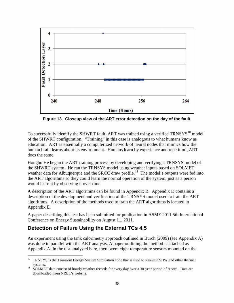
Figure 12 shows how the ART system flags conditions that are out of character from normal operation. The x-axis shows a temporal reference from the beginning of the test. The fault detection layer increases proportionally to the degree to which the condition deviates from normal. Again, the numbers on the x-axis represent hours from the start of the test. The arrow on the graph points to the time of the induced fault. Figure 13 is a closeup view.

Figure 12. ART error detection during the test period.

38

Figure 13. Closeup view of the ART error detection on the day of the fault.

To successfully identify the SHWRT fault, ART was trained using a verified TRNSYS10

Hongbo He began the ART training process by developing and verifying a TRNSYS model of the SHWRT system. He ran the TRNSYS model using weather inputs based on SOLMET weather data for Albuquerque and the SRCC draw profile.

model of the SHWRT configuration. “Training” in this case is analogous to what humans know as education. ART is essentially a computerized network of neural nodes that mimics how the human brain learns about its environment. Humans learn by experience and repetition; ART does the same.

11

A description of the ART algorithms can be found in Appendix B. Appendix D contains a description of the development and verification of the TRNSYS model used to train the ART algorithms. A description of the methods used to train the ART algorithms is located in Appendix E.

The model’s outputs were fed into the ART algorithms so they could learn the normal operation of the system, just as a person would learn it by observing it over time.

A paper describing this test has been submitted for publication in ASME 2011 5th International Conference on Energy Sustainability on August 11, 2011.

Detection of Failure Using the External TCs 4,5

An experiment using the tank calorimetry approach outlined in Burch (2009) (see Appendix A) was done in parallel with the ART analysis. A paper outlining the method is attached as Appendix A. In the test analyzed here, there were eight temperature sensors mounted on the 10 TRNSYS is the Transient Energy System Simulation code that is used to simulate SHW and other thermal

systems. 11 SOLMET data consist of hourly weather records for every day over a 30-year period of record. Data are

downloaded from NREL’s website.

39

sidewall of the inner vessel, at roughly the same height of the immersed tank sensors used in the ART data analysis. Figure 14 shows the location of the sensors. The sensors were mounted by cutting away a ~2-inch × 2-inch piece of the metal external skin, removing the insulation, epoxying the sensor to the tank wall, and replacing the insulation and skin. There is a separate study of the accuracy of these sensors compared to the immersed sensors (truth) in the next section.

Figure 14. Location of external wall temperature sensors.

40

UNM provided data time series of the external and internal tank sensors, Ttank-environment, Tambient, and Isun, in the plane of the collector. These data were used in the analysis method (see Appendix A). Using these variables improves the accuracy of the predictions considerably, as opposed to when one must “guess” the values. Without such data, Isun is gotten by assuming a clear sky, and using ASHRAE correlations for clear sky to predict that radiation. Removing that restriction by using measured data considerably reduces error in prediction. Of course, without Isun data, one could not diagnose the observed failure with any certainty, as total overcast is an alternative explanation of the abnormal behavior and could certainly occur for two days in a row (the duration of the fault in the data).

The data were averaged into 5-minute bins to reduce data density. Since positive dT/dt is detected numerically as (Ti+1 - Ti+1)/(ti+1 - ti+1), the temperatures need to change outside of the “noise band” to get steady results. The data could have been read in directly and the “specify how many data points to skip” option could have been used, but this bogs the computer down too much. The spreadsheet-based software uses cell formulae rather than the more efficient imbedded programming language.

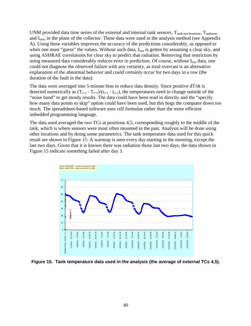
The data used averaged the two TCs at positions 4,5, corresponding roughly to the middle of the tank, which is where sensors were most often mounted in the past. Analysis will be done using other locations and by doing some parametrics. The tank temperature data used for this quick result are shown in Figure 15. A warmup is seen every day starting in the morning, except the last two days. Given that it is known there was radiation those last two days, the data shown in Figure 15 indicate something failed after day 3.

Figure 15. Tank temperature data used in the analysis (the average of external TCs 4,5).

0

10

20

30

40

50

60

70

Wei

ght (

Tank

Tem

p) =

=>

1/7/

2011

22

:15:

03

1/8/

2011

3:

45:0

3

1/8/

2011

9:

15:0

6

1/8/

2011

14

:45:

30

1/8/

2011

20

:15:

33

1/9/

2011

1:

45:3

6

1/9/

2011

7:

15:3

9

1/9/

2011

12

:45:

42

1/9/

2011

18

:15:

42

1/9/

2011

23

:45:

48

1/10

/201

1 5

:15:

48

1/10

/201

1 1

0:45

:54

1/10

/201

1 1

6:15

:57

1/10

/201

1 2

1:46

:00

1/11

/201

1 3

:16:

03

1/11

/201

1 8

:46:

06

1/11

/201

1 1

4:16

:09

1/11

/201

1 1

9:46

:12

1/12

/201

1 1

:16:

15

1/12

/201

1 6

:46:

18

Degr

ees

C

Scroll: Hold SHIFT, move mouse left or rightZoom: Hold CTRL, move mouse left or right

41

When the system was operating as qualitatively expected on the first three days (i.e., warmup each day), there was reasonable agreement between the predicted and the measured Q-to-tank, as shown in Figure 16. The predicted is based upon guesses for the collector properties, tilt, etc. The piping and heat exchanger penalties are not factored in at this time, and that will lower the predicted performance.

Figure 16. Measured versus predicted energy to tank.

The time-series plot of the measured versus predicted Qdot,to-tank is shown in Figure 17. This is the key “diagnostics” information, showing what is expected to happen based upon the collector, tank return temperature (given from the data, not normally known), and weather (radiation, Tamb were put in directly from the data, not normally known). There is no time displayed, but the rough time is clear enough from the data. It is evident that measured and predicted power to tank tracks reasonably well through the first three days of the test having solar incidence, 1/8 through 1/10. However, 1/11 and 1/12 show that something happened to destroy the correlation between the measured and predicted between 1/10 and 1/11. There is no indication as to exactly when the fault occurred. It can be inferred only that between the end of solar day 1/10 and the start of the next solar day (1/11) something occurred to cause the tank to no longer see the expected temperature increases. If the failure had been done in mid-day, the time when the fault occurred would be seen precisely.

Lastly, each night allowed the inference of a tank UA. The UA is inferred via the ln(DT1/DT2) approach that assumes Tenvironment (Tenv) is constant, and so the fact that Tenv varied so much is a minor issue. The method averages Tenv over the time interval, but this is not rigorous. The method might be changed to give UA as f(time) that allows Tenv to vary, but that is not a high priority at the moment. It is also an issue that draws did not allow much of a time window to see the decay, and more than 2 °C decay was not seen in the three valid nights of data (see Figure 18). The tank UA analysis period was set to 4 hours starting at 1 a.m., each night. The average UA was 6.4 ± 0.6 W/C, with error given as the standard deviation of the three data points. Given the varying Tenv, about 1 need to be added to that 0.6, based upon variations in inferred UA seen with different time windows set; the method shows UAtank = ~6.4 ± 1.6 W/C.

y = 0.76x

0

500

1000

1500

2000

2500

3000

3500

0 500 1000 1500 2000 2500 3000 3500

Mea

sure

d En

ergy

to T

ank

(Wat

ts)

Predicted Energy to Tank (Watts)

42

Figure 17. Measured versus predicted Qto-tank, as a line plot.

Figure 18. Tank UA on three successive nights

(fourth night did not pass the screens for robustness).

An issue that is germane to any method that works without weather data: the expected response cannot be known in any finely-time-resolved sense because the irradiance is not known. As such, any method must base its inference probabilistically: what is probability as a function of time duration of a stretch of weather with constantly low irradiance? Until the answer to this question is known, any method cannot say much about failure because there is no grounded expectation.

0.0

500.0

1000.0

1500.0

2000.0

2500.0

3000.0

3500.0

1 34 67 100

133

166

199

232

265

298

331

364

397

430

463

496

529

562

595

628

661

694

727

760

793

826

859

892

925

958

991

1024

1057

1090

1123

1156

1189

1222

1255

1288

1321

1354

Qto

-tan

k, [W

]Measured vs. Predicted Qto-tank

Measured

Predicted

0.00

1.00

2.00

3.00

4.00

5.00

6.00

7.00

8.00

1/0

0:00

7/18

0:0

0

2/3

0:00

8/22

0:0

0

3/10

0:0

0

9/26

0:0

0

4/14

0:0

0

10/3

1 0:

00

5/18

0:0

0

(W/d

egC)

Tank UA

Predicted Measured

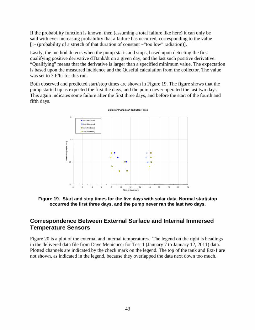
43

If the probability function is known, then (assuming a total failure like here) it can only be said with ever increasing probability that a failure has occurred, corresponding to the value [1- (probability of a stretch of that duration of constant ~”too low” radiation)].

Lastly, the method detects when the pump starts and stops, based upon detecting the first qualifying positive derivative dTtank/dt on a given day, and the last such positive derivative. “Qualifying” means that the derivative is larger than a specified minimum value. The expectation is based upon the measured incidence and the Quseful calculation from the collector. The value was set to 3 F/hr for this run.

Both observed and predicted start/stop times are shown in Figure 19. The figure shows that the pump started up as expected the first the days, and the pump never operated the last two days. This again indicates some failure after the first three days, and before the start of the fourth and fifth days.

Figure 19. Start and stop times for the five days with solar data. Normal start/stop

occurred the first three days, and the pump never ran the last two days.

Correspondence Between External Surface and Internal Immersed Temperature Sensors

Figure 20 is a plot of the external and internal temperatures. The legend on the right is headings in the delivered data file from Dave Menicucci for Test 1 (January 7 to January 12, 2011) data. Plotted channels are indicated by the check mark on the legend. The top of the tank and Ext-1 are not shown, as indicated in the legend, because they overlapped the data next down too much.

0

5

10

150 2 4 6 8 10 12 14 16 18 20 22 24

Julia

n D

ay (D

ay o

f Yea

r)

Time of Day (hours)

Collector Pump Start and Stop Times

Start (Measured)

Stop (Measured)

Start (Predicted)

Stop (Predicted)

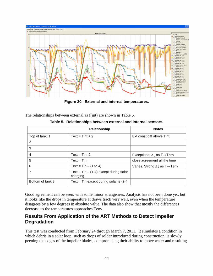
44

Figure 20. External and internal temperatures.

The relationships between external as f(int) are shown in Table 5. Table 5. Relationships between external and internal sensors.

Relationship Notes

Top of tank: 1 Text = Tint + 2 Ext const diff above Tint 2 3 4 Text = Tin -2 Exceptions; ∆↓ as T→Tenv 5 Text = Tin close agreement all the time 6 Text = Tin – (1 to 4) Varies. Strong ∆↓ as T→Tenv 7 Text – Tin – (1-4) except during solar

charging

Bottom of tank 8 Text = Tin except during solar is -2-4

Good agreement can be seen, with some minor strangeness. Analysis has not been done yet, but it looks like the drops in temperature at draws track very well, even when the temperature disagrees by a few degrees in absolute value. The data also show that mostly the differences decrease as the temperatures approaches Tenv.

Results From Application of the ART Methods to Detect Impeller Degradation

This test was conducted from February 24 through March 7, 2011. It simulates a condition in which debris in a solar loop, such as drops of solder introduced during construction, is slowly peening the edges of the impeller blades, compromising their ability to move water and resulting

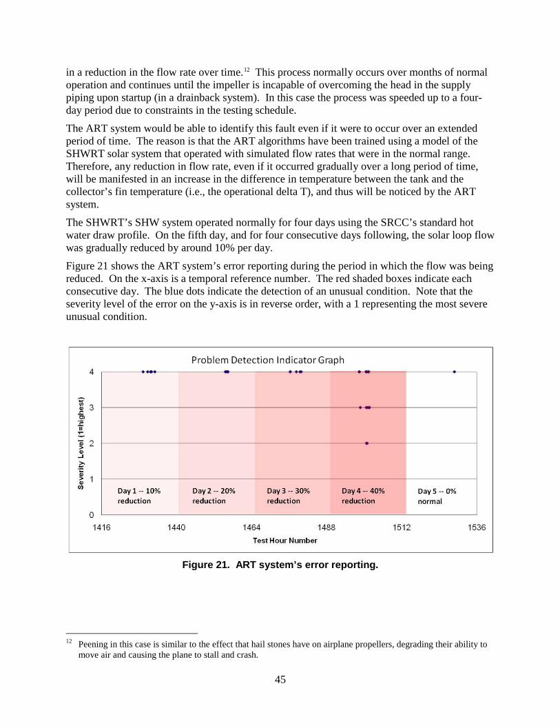
45

in a reduction in the flow rate over time.12

The ART system would be able to identify this fault even if it were to occur over an extended period of time. The reason is that the ART algorithms have been trained using a model of the SHWRT solar system that operated with simulated flow rates that were in the normal range. Therefore, any reduction in flow rate, even if it occurred gradually over a long period of time, will be manifested in an increase in the difference in temperature between the tank and the collector’s fin temperature (i.e., the operational delta T), and thus will be noticed by the ART system.

This process normally occurs over months of normal operation and continues until the impeller is incapable of overcoming the head in the supply piping upon startup (in a drainback system). In this case the process was speeded up to a four-day period due to constraints in the testing schedule.

The SHWRT’s SHW system operated normally for four days using the SRCC’s standard hot water draw profile. On the fifth day, and for four consecutive days following, the solar loop flow was gradually reduced by around 10% per day.

Figure 21 shows the ART system’s error reporting during the period in which the flow was being reduced. On the x-axis is a temporal reference number. The red shaded boxes indicate each consecutive day. The blue dots indicate the detection of an unusual condition. Note that the severity level of the error on the y-axis is in reverse order, with a 1 representing the most severe unusual condition.

Figure 21. ART system’s error reporting.

12 Peening in this case is similar to the effect that hail stones have on airplane propellers, degrading their ability to

move air and causing the plane to stall and crash.

46

As can be seen, the ART system begins to detect unusual conditions as soon as the flow was reduced. By the fourth day, the system has escalated the level of severity significantly. When the flow was reset to its normal range, the number of detected unusual conditions dropped dramatically.

The ART algorithms used only those temperature sensors that would normally be involved in normal control of an SHW system: the collector plate temperature and the tank outlet temperature. The flow sensor was not included in its sensor set. The four conditions that the ART algorithms used included (1) the collector plate temp, (2) the tank outlet temperature, (3) the difference between the plate and tank temperatures (delta T), and (4) the rate of change of the plate temperature (time derivative).

The ability to predict a component failure on an SHW system is a technological breakthrough, representing a capability that does not exist in any SHW controller today and heretofore was thought to be very difficult to achieve. This predictive ability can lead to higher system reliability because components can be replaced before they fail, at a time when the system would normally be down.

Much more work is needed to verify the ability of ART to predict failures. In this case a process that normally evolves over months or years was condensed into four days. It is unknown whether these ART algorithms would have been able to detect this degradation over a longer period of time. It is probably the case that this degradation would have been detected over a long period of time as long as the training covered that period. However, additional experimental work is needed to prove it.

ART algorithms are written in a modern language, such as C++. Thus, they can be easily integrated into modern controllers, most of which are microprocessor-based. Since no additional sensors are required in the ART system beyond what is normally used, the addition of these algorithms provides significant intelligence to controllers at very low cost.

However, there are many issues that must be addressed before the ART algorithms can be implemented in a controller, such as how they will learn to differentiate between a true fault and one in which a system owner is on vacation.

The Calorimetric method was not applied to the degradation experiment.

47

8. CONCLUSIONS AND RECOMMENDATIONS

The following are conclusions from this work:

• All of the objectives of the UNM and BSI contracts were met or exceeded, although the labor required to bring the project to fruition surpassed the original expectations by around an order of magnitude.

• Both the ART and Burch’s Calorimetric methods successfully identified failures. ART uses the same sensors as are normally used to control an SHW system. The Calorimetric method uses two additional temperature sensors that are attached to the outside skin of the solar tank.

• The ART methodology demonstrated a rudimentary capability to anticipate a failure condition, one in which a pump impeller is degrading due to debris in the line. However, the test period of four days was a condensation of a much longer period in which this type of degradation would normally occur. It is unknown whether ART could effectively detect the same level of degradation over a longer period of time. Nonetheless, the results are very encouraging.

• Catastrophic failures are relatively easy to detect, but predicting failures is much more valuable. However, predicting failures is many times more difficult and requires careful training of the ART algorithms.

• The resulting testbed has much more capability than what was originally envisioned for reliability testing. It can be used for thermal tests as well, and some will be conducted soon.

• The results of this work may form the basis for developing an advanced generation controller, one that can not only detect and predict faults, but can also help guide the operator to a specific problem area. Since the ART algorithms can be written in standard computer languages, such as C++, they can be easily integrated into most modern SHW controllers, most of which are microprocessor-based. The functional specifications for such a controller are contained in Appendix G.

• Many of the new techniques and concepts developed in this solar thermal project—much of which will involve new theory—will likely be applicable to other small generators. An SHW system is fundamentally an intermittent generator and differs from others in the makeup of its components and the final energy product that it generates. Knowledge gained from work on solar thermal generators could help to define new approaches to reliability of all small generators and improve their standing among the more traditional generators.

• A comparison between the external sensors on the tank side-wall and the internal sensors immersed in the tank was made. Eliminating the cases where the thermocouple was mounted on the wraparound heat exchanger, there was good agreement between the internal and external sensors. This comparison provides an indirect validation of the calorimetric method when using external sensors. The external sensors generally read slightly lower than the immersed sensors, about 1 to 2 ºC. The difference disappeared as the tank approached ambient temperatures. There was also some difference in registering

48

sudden transitions, with the wall sensors lagging the transient as seen by the immersed sensor.

• ART-based fault detection should be applicable to larger, more complex systems, including building-scale solar cooling and heating, as well as other HVAC applications. Attempts to do so are under way at UNM.

• The following are the lessons that the UNM/BSI team learned in the course of this project:

The investment in higher-quality equipment saves time and effort over the longer term. For example, a low-cost flow meter was procured for the load loop, but its output was difficult to handle in the VI. The costs for programming the LabView VI to accurately capture the signals it produced far exceeded the initial savings.

The level of effort and degree of complexity to develop the LabView VI to control the SHWRT was grossly underestimated. Even from an early stage the challenge was well beyond the expertise of the team, especially the student who was attempting to develop the software. An expert from SNL provided many hours of expertise to bring the system into operation. This phase of the test program must be carefully planned in any future research program involving the SHWRT.

Used computer equipment for controlling the SHWRT was inappropriate for the task. Hardware failures and a cadre of strange and unusual software errors complicated the development of the LabView software because when problems occurred it was often difficult to trace the source of the problem. New equipment should be used for this critical function.

Similarly, the team began the project with an older version of LabView, which had many shortcomings. Special programming techniques were needed to circumvent these shortcomings. The latest version of the LabView software should be implemented from the outset of the project because it will save time in the long term.

The labor anticipated for the project was grossly underestimated during the planning phase. Thus the construction period was much longer than anticipated. Unlike SNL, which employs numerous tradespeople and technicians, UNM researchers performed all of the labor to construct the SHWRT. This situation must be considered for any new project at UNM.

The effectiveness of the ART algorithms depends on training using an accurate model of the system to which they will be applied. It is essential to ensure that the model is fully verified before any training is begun. The team wasted some time initially by moving too quickly to train the algorithms before the model was fully verified.

A thorough understanding of the ART theory is required before it can be applied. The team struggled at times with the application because all members did not have a common understanding of the theory.

49

The selection of the proper parameters for use by the ART algorithms is critical for application, but at this time is more of an art than a science. For example, even though there were only two temperature parameters available to the ART system for its tests (the collector fin temperature and the tank outlet temperature), there are many combinations of these parameters that can be derived from them. Consider these possibilities: (1) the temperature difference between the sensors, (2) the time derivative of the fin temperature, (3) the time derivative of the outlet temperature, (4) the time derivative of the difference in the temperatures, (5) the time of day, and so on. At present the only method to select the appropriate parameters is through the use of a verified system simulation model, such as the TRNSYS, and human intuition.

Since the team was inexperienced with the ART methodology, the time required for training the algorithms was longer than anticipated.

The TRNSYS model that was used was not an exact duplicate of the SHWRT system. As a result, many runs and much manipulation was needed to achieve the level of accuracy needed for the ART training. It would be preferable to invest in the appropriate TRNSYS software at the outset. For example, had the team updated to TRNSYS 17 software (from 16), the level of effort would have been substantially lower.

The following are recommended actions:

1. Work should continue on the development of the two methods for failure detection and failure prediction. Specifically, additional experiments should be conducted to test a wide array of failures that might likely occur in a SHW system.

2. Work should continue on the development of the predictive ability of the ART algorithms, especially to develop refined methods for training them in preparation for predicting faults and failures.

3. The ART system of algorithms has potential beyond SHW that should be explored. Specifically, they might effectively be applied in surety microgrids of the type being developed by SNL. In these microgrids numerous small generators could productively employ the predictive capabilities of the ART algorithms to ensure continually high reliability.

4. Eventually the ART neural networks could be trained using real-time data from an actual system operation in addition to that from a model. This is a requisite for ART to be applicable in modern controller. However, additional work is needed to determine the optimal amount and type of training that is needed for these algorithms to be included in controllers.

5. The team should move forward with plans to develop a new state-of-the-art controller that incorporates the ART and Calorimetric methods that were tested in this project.

50

REFERENCES

1. Assembly and Comparison of Available Solar Hot Water System Reliability Databases and Information, SAND2009-2757. Sandia National Laboratories, Albuquerque, NM, May 2009.

2. I. Bazovsky, Reliability Theory and Practice, Chapter 3, The Exponential Case of Chance Failures. Prentice Hall, Inc., Englewood Cliffs, New Jersey, 1961.

3. J. Burch, et al., Field Monitoring of Solar Domestic Hot Water Systems Based on Simple Tank Temperature Measurements, NREL Technical Paper, NREL/TP-472-7854, December 1995.

4. G.A. Carpenter and S. Grossberg, Adaptive resonance theory, The Handbook of Brain Theory and Neural Networks, vol. 2, pp. 87-90, 2003.

5. T.P. Caudell, Hybrid optoelectronic adaptive resonance theory neural processor, ART1, Applied Optics, vol. 31, pp. 6220-6229, 1992.

6. T.P. Caudell, S.D.G. Smith, R. Escobedo, and M. Anderson, NIRS: large scale ART-1 neural architectures for engineering design retrieval, Neural Networks, vol. 7, pp. 1339-1350, 1994.

51

Appendix A. Paper by Jay Burch, et al., Describing the Calorimetric Methodology

(reproduction with written permission of the author)

52

53

Appendix B. Description of the Artificial Resonance Theory That Was Applied to Solar Hot Water Failure Analysis

A fuzzy Adaptive Resonance Theory (ART) neural network has three layers: input layer F0, comparison layer F1, and category layer F2 (see Figure B-1) [1,2]. The number of neurons in layer F0 and layer F1 are the same because each neuron in layer F1 is response to one value of an input pattern pixel in layer F0. Each neuron in layer F2 represents a category. Each neuron in layer F1 is connected to all neurons in layer F2 through bottom-up weights bu

ijw wijbu. Index i

means that the connection between the i-th neuron in layer F1 and the j-th neuron in layer F2. The input patterns and bottom-up weights bu

ijw are analog valued. The input to the j-th neuron in layer F2 from layer F1 is

j

jj w

wIT

+

∧=α

, (B-1)

Figure B-1. ART-1 architecture.

where ∧ is the fuzzy MIN operator defined by ( ) ( ) ( ),,,,,min 1 Njjjiii wwwYXYX ==∧ X

is the 1-norm ∑=

=N

iiXX

1

, α is the choice parameter, and N is the pixels of the input pattern.

54

The default value of the neurons in layer F2 is ‘0’, except for the neuron receiving the maximum Tj from layer F1. That neuron is the winning neuron in F2 layer, and we label it J. The output of the neuron J is ‘1’,

if j= J , yj=1

else, yj=0 (B-2)

Each neuron in F2 layer is connected to all the neurons in F1 layer through top-down weights tdjiw , then the input of the i-th neuron in F1 layer is

∑=

===M

j

tdJij

tdjii NiwywV

1,,1, (B-3)

A vigilance subsystem that is formed by the reset controller in Figure B-2 checks the appropriateness of the active F2 neuron.

ρ≥∧IwI J , (B-4)

where ρ is the vigilance parameter.

If the Equation (B-4) is not true, then the vigilance subsystem will reset the actual active F2 category J and forcing TJ = 0. Another active category in F2 layer will be chosen with maximum Tj and the vigilance criterion will be checked again. This process will not stop until an active category J in F2 layer satisfies the vigilance criterion.

The fuzzy ART training algorithm is shown in Figure B-2. As a result of training, each pattern in the data sets has a corresponding category – represented by the active node in F2 layer.

The current input pattern is compared to the nodes in layer F2. If none of the nodes in layer F2 match the input pattern sufficiently, then a new F2 node or category will be created to store the input pattern. When the current input pattern matches one of the nodes in layer F2 adequately, the long term memory traces or adaptive weights associated with the node will be modified to store the information of the current input pattern. Therefore, when a new pattern arises, fuzzy ART learns to categorize it without forgetting the previously learned patterns.

A four-layer hierarchical ART neural network, as shown in Figure B-3, is a cascade of fuzzy ART modules [3,4]. This hierarchical ART neural network creates the most general level of categories first and then divides these categories into more specific ones. It learns to categorize the input patterns with higher vigilance parameters compared to the previous active fuzzy ART module that is connected, through the hierarchical links, to the active F2 nodes. There are different vigilance parameters in each layer; the higher the level of the layer the higher the vigilance parameters. The objective is to detect different kinds of failures and prioritize those failures based on severity. Alarms can be created to indicate the level of severity.

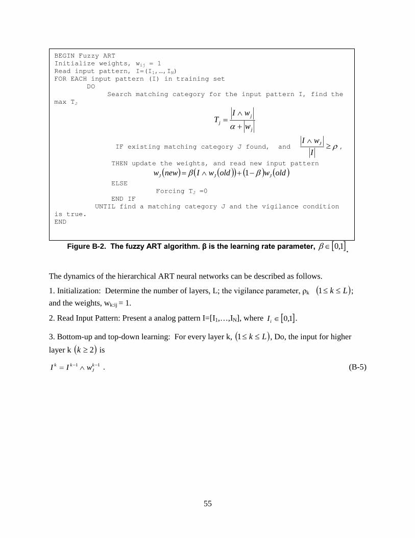
55

Figure B-2. The fuzzy ART algorithm. β is the learning rate parameter, [ ]1,0∈β .

The dynamics of the hierarchical ART neural networks can be described as follows.

1. Initialization: Determine the number of layers, L; the vigilance parameter, ρk ( )Lk ≤≤1 ; and the weights, wk:ij = 1.

2. Read Input Pattern: Present a analog pattern I=[I1,…,IN], where [ ]1,0∈iI .

3. Bottom-up and top-down learning: For every layer k, ( )Lk ≤≤1 , Do, the input for higher layer k ( )2≥k is

11 −− ∧= kJ

kk wII . (B-5)

BEGIN Fuzzy ART Initialize weights, wij = 1 Read input pattern, I=(I1,…,IN) FOR EACH input pattern (I) in training set DO Search matching category for the input pattern I, find the max TJ

j

jj w

wIT

+

∧=α

IF existing matching category J found, and ρ≥∧IwI J ,

THEN update the weights, and read new input pattern

( ) ( )( ) ( ) ( )oldwoldwIneww JJJ ββ −+∧= 1

ELSE Forcing TJ =0 END IF UNTIL find a matching category J and the vigilance condition is true. END

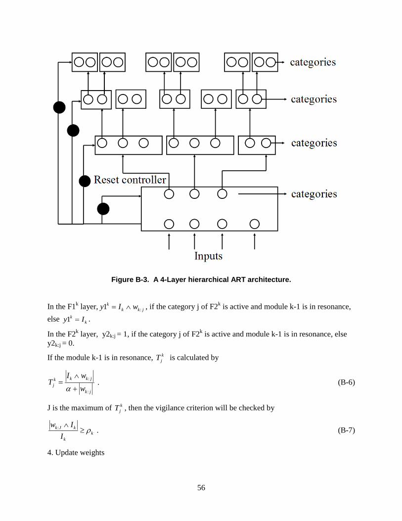
56

Figure B-3. A 4-Layer hierarchical ART architecture.

In the F1k layer, jkkk wIy :1 ∧= , if the category j of F2k is active and module k-1 is in resonance,

else kk Iy =1 .

In the F2k layer, y2k:j = 1, if the category j of F2k is active and module k-1 is in resonance, else y2k:j = 0.

If the module k-1 is in resonance, kjT is calculated by

jk

jkkkj w

wIT

:

:

+

∧=α

. (B-6)

J is the maximum of kjT , then the vigilance criterion will be checked by

kk

kJk

IIw

ρ≥∧: . (B-7)

4. Update weights

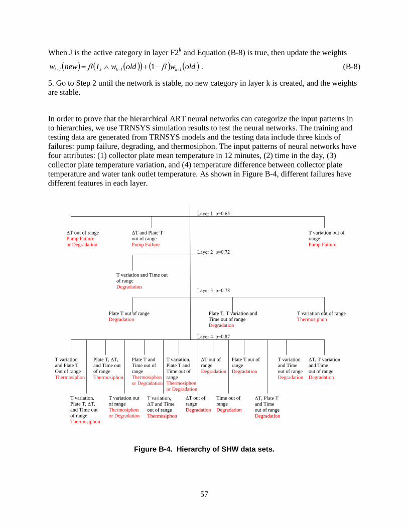
57

When J is the active category in layer F2k and Equation (B-8) is true, then update the weights

( ) ( )( ) ( ) ( )oldwoldwIneww JkJkkJk ::: 1 ββ −+∧= . (B-8)

5. Go to Step 2 until the network is stable, no new category in layer k is created, and the weights are stable.

In order to prove that the hierarchical ART neural networks can categorize the input patterns in to hierarchies, we use TRNSYS simulation results to test the neural networks. The training and testing data are generated from TRNSYS models and the testing data include three kinds of failures: pump failure, degrading, and thermosiphon. The input patterns of neural networks have four attributes: (1) collector plate mean temperature in 12 minutes, (2) time in the day, (3) collector plate temperature variation, and (4) temperature difference between collector plate temperature and water tank outlet temperature. As shown in Figure B-4, different failures have different features in each layer.

Figure B-4. Hierarchy of SHW data sets.

Layer 1 ρ=0.65

ΔT out of range Pump Failure or Degradation

ΔT and Plate T out of range Pump Failure

T variation out of range Pump Failure

T variation and Time out of range Degradation

Layer 2 ρ=0.72

Layer 3 ρ=0.78

Plate T out of range Degradation

Plate T, T variation and Time out of range Degradation

T variation out of range Thermosiphon

Layer 4 ρ=0.87

T variation and Plate T Out of range Thermosiphon

T variation, Plate T, ΔT, and Time out of range Thermosiphon

Plate T, ΔT, and Time out of range Thermosiphon

T variation out of range Thermosiphon or Degradation

Plate T and Time out of range Thermosiphon or Degradation

T variation, Plate T and Time out of range Thermosiphon or Degradation

ΔT out of range Degradation

T variation, ΔT and Time out of range Thermosiphon

ΔT out of range Degradation

ΔT, Plate T and Time out of range Degradation

Time out of range Degradation

Plate T out of range Degradation

T variation and Time out of range Degradation

ΔT, T variation and Time out of range Degradation

58

Figure B-4 shows the hierarchy of SHW data sets generalized by a four-layer hierarchical ART neural network. The vigilance levels were ρ1 = 0.65, ρ2 =0.72, ρ3 = 0.78, and ρ4 =87. In this example, 3, 1, 3, and 14 categories are created in layers 1, 2, 3 and 4 respectively.

The training data for the hierarchical ART neural networks is from a TRNSYS fault-free model, as shown above. For Albuquerque, 38 years’ data is available; therefore, the fault-free results of the SHW system under different weather conditions will be included. The inputs to the hierarchical ART neural networks are the normalization of collector plate mean temperature in 12 minutes, time in the day, collector plate temperature variation, and temperature difference between collector plate temperature and water tank outlet temperature. Additionally, the collector outlet mean temperature can be in 12 minutes, 18 minutes, or other intervals; the time range depends on the SHW system. All the input patterns are presented to the neural network as eight-element analogy vectors with the same norm of 4.

References

1. G.A. Carpenter and S.A. Grossberg, Massively Parallel Architecture for a Self-organizing Neural Pattern Recognition Machine, Computer Vision, Graphics, and Image Processing, vol. 37, pp. 54-115, 1987.

2. G.A. Carpenter, S. Grossberg, and D.B. Rosen, Fuzzy art: Fast stable learning and categorization of analog patterns by an adaptive resonance system, Neural Networks, vol. 4(6), pp. 759-71, 1991.

3. T.P. Caudell, S.D.G. Smith, R. Escobedo, and M. Anderson, NIRS: Large scale ART-1 neural architectures for engineering design retrieval, Neural Networks, vol. 7(9), pp. 1339-1350, 1994.

4. T.P. Caudell and D.S. Newman, An adaptive resonance architecture to define normality and detect novelties in time series and databases, Proceedings of the INNS World Congress on Neural Networks, Portland, vol. IV, pp. 166-176, 1993.

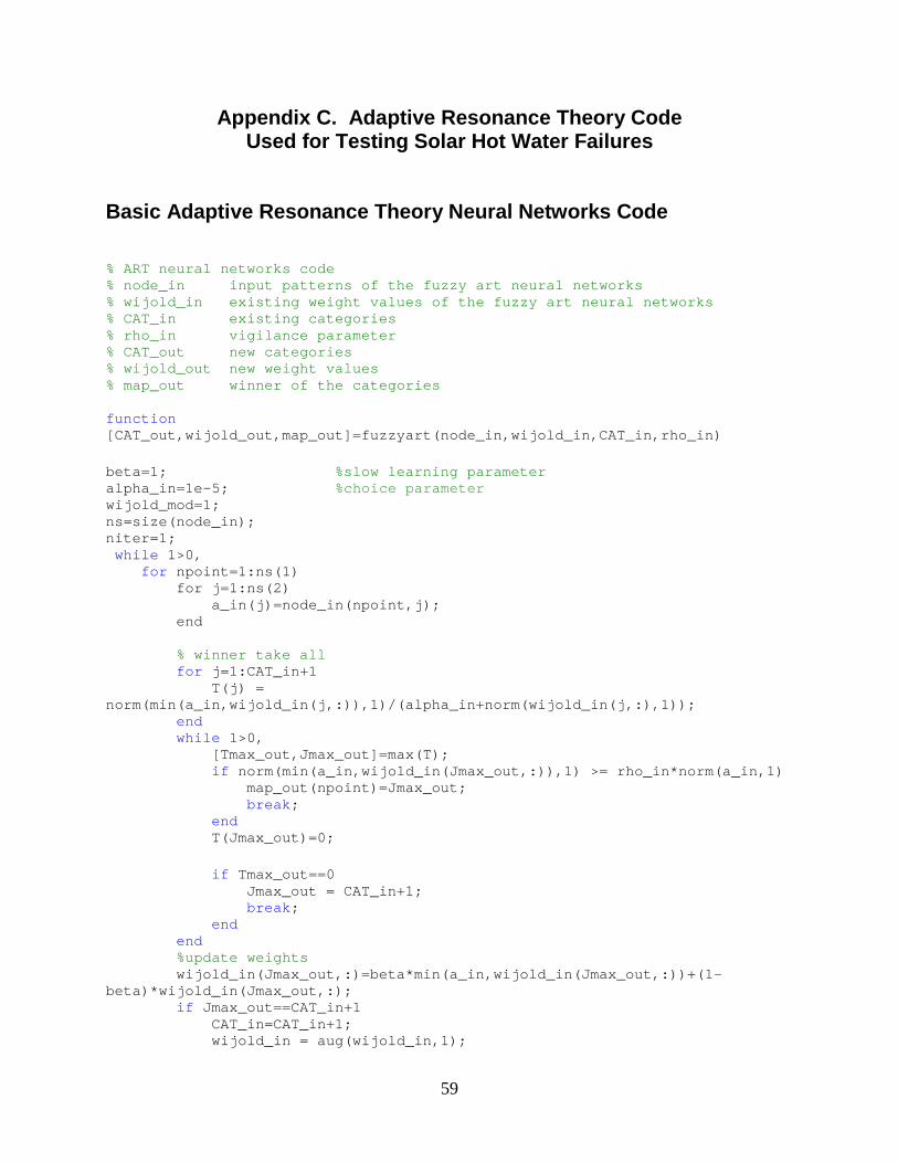
59

Appendix C. Adaptive Resonance Theory Code Used for Testing Solar Hot Water Failures

Basic Adaptive Resonance Theory Neural Networks Code

% ART neural networks code % node_in input patterns of the fuzzy art neural networks % wijold_in existing weight values of the fuzzy art neural networks % CAT_in existing categories % rho_in vigilance parameter % CAT_out new categories % wijold_out new weight values % map_out winner of the categories function [CAT_out,wijold_out,map_out]=fuzzyart(node_in,wijold_in,CAT_in,rho_in) beta=1; %slow learning parameter alpha_in=1e-5; %choice parameter wijold_mod=1; ns=size(node_in); niter=1; while 1>0,

for npoint=1:ns(1) for j=1:ns(2) a_in(j)=node_in(npoint,j); end

% winner take all for j=1:CAT_in+1 T(j) = norm(min(a_in,wijold_in(j,:)),1)/(alpha_in+norm(wijold_in(j,:),1)); end while 1>0, [Tmax_out,Jmax_out]=max(T); if norm(min(a_in,wijold_in(Jmax_out,:)),1) >= rho_in*norm(a_in,1) map_out(npoint)=Jmax_out; break; end T(Jmax_out)=0; if Tmax_out==0 Jmax_out = CAT_in+1; break; end end %update weights wijold_in(Jmax_out,:)=beta*min(a_in,wijold_in(Jmax_out,:))+(1-beta)*wijold_in(Jmax_out,:); if Jmax_out==CAT_in+1 CAT_in=CAT_in+1; wijold_in = aug(wijold_in,1);

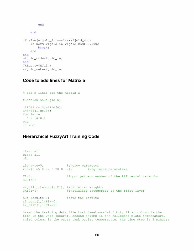
60

end end if size(wijold_in)==size(wijold_mod) if norm(wijold_in-wijold_mod)<0.0002 break; end end wijold_mod=wijold_in; end CAT_out=CAT_in; wijold_out=wijold_in;

Code to add lines for Matrix a

% add n lines for the matrix a function aa=aug(a,n) [lines,cols]=size(a); u=ones(1,cols); for i=1:n a = [a;u]; end aa = a;

Hierarchical FuzzyArt Training Code

clear all close all clc alpha=1e-5; %choice parameter rho=[0.65 0.72 0.78 0.87]; %vigilance parameters F1=8; %input pattern number of the ART neural networks S=F1/2; wij01(1,:)=ones(1,F1); %initialize weights CAT01=0; %initialize categories of the first layer out_results=0; %save the results a1_test(1,1:F1)=0; a2_test(1,1:F1)=0; %read the training data file train5weeksmar3min2.txt, first column is the time in the year (hours), second column is the collector plate temperature, third column is the water tank outlet temperature, the time step is 3 minutes

61

[node(:,1),node(:,2),node(:,3)]= textread('train5weeksmar3min2.txt','%f %f %f'); snode=size(node); % in this part we will get the input patterns for the neural networks: collector plate mean temperature in 12 minutes, delta temperature between collector plate temperature and water tank outlet temperature, the time in the day, variation of the collector plate temperature for i=1:snode(1,1) for j=1:snode(1,2) node2(i,j)=node(i,j); end end for i=1:snode(1,1) node3(i,1)=node2(i,1); end for i=4:snode(1,1) node3(i,2)=(node2(i,2)+node2(i-1,2)+node2(i-2,2)+node2(i-3,2))/4; node3(i,3)=(node2(i,3)+node2(i-1,3)+node2(i-2,3)+node2(i-3,3))/4; end for i=4:snode(1,1) node3(i,3)=node3(i,2)-node3(i,3); end for i=1:3 node3(i,2)=node3(4,2); node3(i,3)=node3(4,3); end for i=3:snode(1,1) node3(i,snode(1,2)+1)=(3*node2(i,2)-4*node2(i-1,2)+node2(i-2,2))/6; node3(i,snode(1,2)+2)=(3*node2(i,3)-4*node2(i-1,3)+node2(i-2,3))/6; end for i=1:2 node3(i,snode(1,2)+1)=node3(3,snode(1,2)+1); node3(i,snode(1,2)+2)=node3(3,snode(1,2)+2); end for i=1:snode(1,1) node3(i,snode(1,2)+3)=rem(node2(i,1),24)/24; end for i=1:snode(1,1) node3(i,snode(1,2)+4)=node3(i,2); node3(i,snode(1,2)+5)=node3(i,3); end snode=size(node3); clear node2 I j

62

% normalization of the input patterns for i=1:snode(1,2)-1 min0(i)=min(node3(:,i+1)); max0(i)=max(node3(:,i+1)); end max0(1)=max0(1)+5; max0(2)=max0(2)+5; max0(6)=max0(6)+5; max0(7)=max0(7)+5; min0(1)=min0(1)-5; min0(2)=min0(2)-5; min0(6)=min0(6)-5; min0(7)=min0(7)-5; for i=1:snode(1,1) for j=2:snode(1,2) node3(i,j)=(node3(i,j)-min0(j-1))/(max0(j-1)-min0(j-1)); end end ns=size(node3); np=ns(1); % set the input patterns for point=1:1:np out_results(point,1)=node3(point,1); out_results(point,2)=node3(point,2); out_results(point,3)=node3(point,3); out_results(point,4)=node3(point,6); out_results(point,5)=node3(point,4); a0(point,1)=node3(point,2); a0(point,2)=1-a0(point,1); a0(point,3)=node3(point,3); a0(point,4)=1-a0(point,3); a0(point,5)=node3(point,6); a0(point,6)=1-a0(point,5); a0(point,7)=node3(point,4); a0(point,8)=1-a0(point,7); end clear node point snode(1,2)=5; % run 4 layer hierarchical fuzzy ART neural networks training part for k=1:4 if k==1 CAT=CAT01; % first layer categories wijtest=wij01; % first layer weights %call fuzzyart part code [CAT_temp,wijold_temp,map_temp]=fuzzyart(a0,wijtest,CAT,rho(k)); %save results of first layer

63

CAT01=CAT_temp; wij01=wijold_temp; count1(1:CAT01)=0; for point=1:1:np count1(map_temp(point))=count1(map_temp(point))+1; a1_temp{1,map_temp(point)}(1,count1(map_temp(point)))=point; for h=1:F1 a1{1,map_temp(point)}(count1(map_temp(point)),h)=a0(point,h); end out_results(point,snode(1,2)+k)=map_temp(point); end clear CAT_temp wijold_temp map_temp point h end if k==2 CAT12(1:CAT01)=0; % initialize second layer categories for h=1:CAT01 if count1(h)>0 for r=1:count1(h) for t=1:F1 a1_test(r,t)=a1{1,h}(r,t); end end clear r t wij12{1,h}(1,:)=ones(1,F1); %initialize second layer weights wijtest(1,1:F1)=wij12{1,h}(1,1:F1); CAT=CAT12(h); %call fuzzyart part code [CAT_temp,wijold_temp,map_temp]=fuzzyart(a1_test,wijtest,CAT,rho(k)); %save results of second layer CAT12(h)=CAT_temp; [line12,col12]=size(wijold_temp); for r=1:line12 for t=1:col12 wij12{1,h}(r,t)=wijold_temp(r,t); end end clear r t for r=1:count1(h) out_results(a1_temp{1,h}(1,r),snode(1,2)+k)=map_temp(r); end clear wijtest map_temp wijold_temp CAT CAT_temp line12 r a1_test end end clear count1 a1_temp a1 h r t for h=1:CAT01 count2{h}(1:CAT12(h))=0; end clear h

64

for point=1:1:np count2{1,out_results(point,snode(1,2)+k-1)}(1,out_results(point,snode(1,2)+k))=count2{1,out_results(point,snode(1,2)+k-1)}(1,out_results(point,snode(1,2)+k))+1; a2_temp{1,out_results(point,snode(1,2)+k-1)}{1,out_results(point,snode(1,2)+k)}(1,count2{1,out_results(point,snode(1,2)+k-1)}(1,out_results(point,snode(1,2)+k)))=point; for h=1:F1 a2{1,out_results(point,snode(1,2)+k-1)}{1,out_results(point,snode(1,2)+k)}(count2{1,out_results(point,snode(1,2)+k-1)}(1,out_results(point,snode(1,2)+k)),h)=a0(point,h); end end clear point h end if k==3 for h=1:CAT01 CAT23(h,1:CAT12(h))=0; %initialize the third layer categories end clear h for h=1:CAT01 for r=1:CAT12(h) if count2{1,h}(1,r)>0 for t=1:count2{1,h}(1,r) for u=1:F1 a2_test(t,u)=a2{1,h}{1,r}(t,u); end end clear t u wij23{1,h}{1,r}(1,:)=ones(1,F1); %initialize the third layer weights wijtest(1,1:F1)=wij23{1,h}{1,r}(1,1:F1); CAT=CAT23(h,r); %call fuzzy art part code [CAT_temp,wijold_temp,map_temp]=fuzzyart(a2_test,wijtest,CAT,rho(k)); %save results of third layer CAT23(h,r)=CAT_temp; [line23,col23]=size(wijold_temp); for t=1:line23 for u=1:col23 wij23{1,h}{1,r}(t,u)=wijold_temp(t,u); end end clear t u for t=1:count2{1,h}(1,r) out_results(a2_temp{1,h}{1,r}(1,t),snode(1,2)+k)=map_temp(t); end clear a2_test wijtest map_temp wijold_temp CAT_temp t end

65

end end clear count2 a2_temp a2 h r t u for h=1:CAT01 for r=1:CAT12(h) count3{1,h}{1,r}(1,1:CAT23(h,r))=0; end end clear h r for point=1:1:np count3{1,out_results(point,snode(1,2)+k-2)}{1,out_results(point,snode(1,2)+k-1)}(1,out_results(point,snode(1,2)+k))=count3{1,out_results(point,snode(1,2)+k-2)}{1,out_results(point,snode(1,2)+k-1)}(1,out_results(point,snode(1,2)+k))+1; a3_temp{1,out_results(point,snode(1,2)+k-2)}{1,out_results(point,snode(1,2)+k-1)}{1,out_results(point,snode(1,2)+k)}(1,count3{1,out_results(point,snode(1,2)+k-2)}{1,out_results(point,snode(1,2)+k-1)}(1,out_results(point,snode(1,2)+k)))=point; for h=1:F1 a3{1,out_results(point,snode(1,2)+k-2)}{1,out_results(point,snode(1,2)+k-1)}{1,out_results(point,snode(1,2)+k)}(count3{1,out_results(point,snode(1,2)+k-2)}{1,out_results(point,snode(1,2)+k-1)}(1,out_results(point,snode(1,2)+k)),h)=a0(point,h); end end clear point h end if k==4 for h=1:CAT01 for r=1:CAT12(h) CAT34{1,h}(r,1:CAT23(h,r))=0; %initialize the forth layer categories end end clear h r for h=1:CAT01 for r=1:CAT12(h) for t=1:CAT23(h,r) if count3{1,h}{1,r}(1,t)>0 for u=1:count3{1,h}{1,r}(1,t) for v=1:F1 a3_test(u,v)=a3{1,h}{1,r}{1,t}(u,v); end end clear u v wij34{1,h}{1,r}{1,t}(1,:)=ones(1,F1); %initialize 4th layer weights

66

wijtest(1,1:F1)=wij34{1,h}{1,r}{1,t}(1,1:F1); CAT=CAT34{1,h}(r,t); %call fuzzy art part code [CAT_temp,wijold_temp,map_temp]=fuzzyart(a3_test,wijtest,CAT,rho(k)); CAT34{1,h}(r,t)=CAT_temp; [line34,col34]=size(wijold_temp); for u=1:line34 for v=1:col34 wij34{1,h}{1,r}{1,t}(u,v)=wijold_temp(u,v); end end clear u v for u=1:count3{1,h}{1,r}(1,t) out_results(a3_temp{1,h}{1,r}{1,t}(1,u),snode(1,2)+k)=map_temp(u); end clear a3_test wijtest map_temp wijold_temp CAT_temp u end end end end clear count3 a3_temp a3 h r t u v end end clear a0 node3 %save the training results fid = fopen('results_train.txt','wt'); for k=1:np fprintf(fid,'%6.2f %1.6f %1.6f %1.6f %1.6f %2d %2d %2d %2d\n',out_results(k,1),out_results(k,2),out_results(k,3),out_results(k,4),out_results(k,5),out_results(k,6),out_results(k,7),out_results(k,8),out_results(k,9)); end clear k fclose(fid); clear ntest numtest ntest2 ntest3 ttest out_test %read the testing file NN05118_3min.txt, first column is the time in the year (hours), second column is the collector plate temperature, third column is the water tank outlet temperature, the time step is 3 minutes [ntest(:,1),ntest(:,2),ntest(:,3)]= textread(NN05118_3min.txt','%f %f %f'); % in this part we will get the input patterns for the neural networks: collector plate mean temperature in 12 minutes, delta temperature between collector plate temperature and water tank outlet temperature, the time in the day, variation of the collector plate temperature numtest=size(ntest); for i=1:numtest(1,1) for j=1:numtest(1,2)

67

ntest2(i,j)=ntest(i,j); end end clear i j for i=1:numtest(1,1) ntest3(i,1)=ntest2(i,1); end for i=4:numtest(1,1) ntest3(i,2)=(ntest2(i,2)+ntest2(i-1,2)+ntest2(i-2,2)+ntest2(i-3,2))/4; ntest3(i,3)=(ntest2(i,3)+ntest2(i-1,3)+ntest2(i-2,3)+ntest2(i-3,3))/4; end for i=4:numtest(1,1) ntest3(i,3)=ntest3(i,2)-ntest3(i,3); end for i=1:3 ntest3(i,2)=ntest3(4,2); ntest3(i,3)=ntest3(4,3); end for i=3:numtest(1,1) ntest3(i,numtest(1,2)+1)=(3*ntest2(i,2)-4*ntest2(i-1,2)+ntest2(i-2,2))/6; ntest3(i,numtest(1,2)+2)=(3*ntest2(i,3)-4*ntest2(i-1,3)+ntest2(i-2,3))/6; end for i=1:2 ntest3(i,numtest(1,2)+1)=ntest3(3,numtest(1,2)+1); ntest3(i,numtest(1,2)+2)=ntest3(3,numtest(1,2)+2); end for i=1:numtest(1,1) ntest3(i,numtest(1,2)+3)=rem(ntest2(i,1),24)/24; end for i=1:numtest(1,1) ntest3(i,numtest(1,2)+4)=ntest3(i,2); ntest3(i,numtest(1,2)+5)=ntest3(i,3); end numtest=size(ntest3); clear ntest % normalization of the input patterns for i=1:numtest(1,1) for j=2:numtest(1,2) if ntest3(i,j)>max0(j-1) ntest3(i,j)=max0(j-1); elseif ntest3(i,j)<min0(j-1) ntest3(i,j)=min0(j-1); end ntest3(i,j)=(ntest3(i,j)-min0(j-1))/(max0(j-1)-min0(j-1)); end

68

end clear ntest2 numtest(1,2)=5; err_num=1; for m=1:numtest(1,1) %set the input patterns ttest(1)=ntest3(m,2); ttest(2)=1-ttest(1); ttest(3)=ntest3(m,3); ttest(4)=1-ttest(3); ttest(5)=ntest3(m,6); ttest(6)=1-ttest(5); ttest(7)=ntest3(m,4); ttest(8)=1-ttest(7); out_test(m,1)=ntest3(m,1); out_test(m,2)=ntest3(m,2); out_test(m,3)=ntest3(m,3); out_test(m,4)=ntest3(m,6); out_test(m,5)=ntest3(m,4); for i=1:4 %test the input patterns in 4 layers if i==1 CATa=CAT01; wijtest=wij01; end if i==2 CATa=CAT12(out_test(m,numtest(1,2)+i-1)); [line12,col12]=size(wij12{1,out_test(m,numtest(1,2)+i-1)}); for h=1:line12 for r=1:col12 wijtest(h,r)=wij12{1,out_test(m,numtest(1,2)+i-1)}(h,r); end end clear h r end if i==3 CATa=CAT23(out_test(m,numtest(1,2)+i-2),out_test(m,numtest(1,2)+i-1)); [line23,col23]=size(wij23{1,out_test(m,numtest(1,2)+i-2)}{1,out_test(m,numtest(1,2)+i-1)}); for h=1:line23 for r=1:col23 wijtest(h,r)=wij23{1,out_test(m,numtest(1,2)+i-2)}{1,out_test(m,numtest(1,2)+i-1)}(h,r); end end clear h r end if i==4 CATa=CAT34{1,out_test(m,numtest(1,2)+i-3)}(out_test(m,numtest(1,2)+i-2),out_test(m,numtest(1,2)+i-1));

69

[line34,col34]=size(wij34{1,out_test(m,numtest(1,2)+i-3)}{1,out_test(m,numtest(1,2)+i-2)}{1,out_test(m,numtest(1,2)+i-1)}); for h=1:line34 for r=1:col34 wijtest(h,r)=wij34{1,out_test(m,numtest(1,2)+i-3)}{1,out_test(m,numtest(1,2)+i-2)}{1,out_test(m,numtest(1,2)+i-1)}(h,r); end end clear h r end wijtest(CATa+1,1:F1)=1; for r=1:CATa+1 Ti(r)=norm(min(ttest,wijtest(r,:)),1)/(alpha+norm(wijtest(r,:),1)); end clear r while 2>0 [Tmax_test,Jmax_test]=max(Ti); if norm(min(ttest,wijtest(Jmax_test,:)),1)>=rho(i)*norm(ttest,1) break; end if Tmax_test==0 break; end Ti(Jmax_test)=0; end if (Jmax_test==CATa+1) || (Tmax_test==0) out_test(m,numtest(1,2)+i)=9999; %failures category number are 9999 for j=1:numtest(1,2) err_test(err_num,j)=out_test(m,j); end for u=1:i err_test(err_num,numtest(1,2)+u)=out_test(m,numtest(1,2)+u); end clear u if i<4 for u=(i+1):4 err_test(err_num,numtest(1,2)+u)=0; out_test(m,numtest(1,2)+u)=0; end end err_num=err_num+1; break; else out_test(m,numtest(1,2)+i)=Jmax_test; end clear Ti wijtest CATa end end clear ntest3 %save the testing results

70

fid = fopen('results_test.txt','wt'); for k=1:numtest(1,1) fprintf(fid,'%6.2f %1.6f %1.6f %1.6f %1.6f %2d %2d %2d %2d\n',out_test(k,1),out_test(k,2),out_test(k,3),out_test(k,4),out_test(k,5),out_test(k,6),out_test(k,7),out_test(k,8),out_test(k,9)); end clear k fclose(fid); %save the failures results if err_num>0 fid = fopen('errors.txt','wt'); for k=1:err_num-1 fprintf(fid,'%6.2f %1.6f %1.6f %1.6f %1.6f %2d %2d %2d %2d\n',err_test(k,1),err_test(k,2),err_test(k,3),err_test(k,4),err_test(k,5),err_test(k,6),err_test(k,7),err_test(k,8),err_test(k,9)); end clear k fclose(fid); end

71

Appendix D. Description of the Development and Verification of the TRNSYS Model Used in the Solar Hot Water Reliability Testbed

Testing Program

The Adaptive Resonance Theory (ART) neural network must be trained by subjecting it to operational data from a solar hot water (SHW) system. However, actual operational data did not exist for this process. Instead, an SHW system model was used to generate simulated data. TRNSYS is a transient systems simulation program with a modular structure. It is applicable for use in modeling solar thermal systems and has a long track record for accuracy. This system was used to develop a model of the Solar Hot Water Reliability Testbed (SHWRT) SHW system.

Figure D-1. Diagrams of the modeled and actual tank in the SHW system

TRNSYS contains substantial libraries of components that can be selected for configuration into a modular system. These components include solar collectors, pumps, water tank storage, and others.

Ideally the model should be an exact representation of the real system. In reality, it was impossible to match the model to the system because some components in the system had no corollary component within TRNSYS. Tank type 534 is one from the TRNSYS library that matched the SHWRT’s tank most closely, but the heat exchanger is different. As shown in

Heat Exchanger

Water tank in TRNSYS model

Heat Exchanger

Water tank in SHWRT system

72

Figure D-1, the heat exchanger of type 534 is immersed in the water tank, but the heat exchanger in the SHWRT’s tank consists of a copper tube coiled around the outside of the tank.13

The time frame and resources for the project did not allow for the tank/heat exchange system to be created for the TRNSYS model.

14

There are eight temperature sensors in the water tank from bottom to top, as described in Section 6 of this report. In the TRNSYS model the water tank is divided into eight zones, each representing an equal portion of the tank from the bottom to the top. Each node roughly corresponds to the placement of the thermocouples in the tank.

Therefore, the team selected tank type 534 for use in the modeling. The input parameters for the type 534 tank model within the TRNSYS code were adjusted based on trial and error comparisons until its predicted behavior reasonably mirrored the real system. For example, the heat transfer coefficients for each of the eight nodes of the tank were adjusted until the modeled results approximated the measured ones. Clearly this is not optimal, but was about all that could be done under the circumstances.

The upper four zones perform very similarly to the real zones, but the lower four zones are slightly different because the heat exchanger is located in the lower part of the water tank. The wrap-around heat exchanger displaced insulation in the bottom portion of the tank, resulting in more heat loss in that part of the tank than in the upper half. These nuances were incorporated into the model by adjusting the input parameters until the modeled behavior of the tank reasonably represented the actual behavior.

A collector model that exactly matched the one used in the SHWRT was not available in the TRNSYS Thermal Energy System Specialists (TESS) library. Therefore, the model that most closely matched the real one (type 564) was selected for use.

This collector model required a number of input parameters to be defined. Some of these parameters were based on measurements taken from the collector directly, such as its physical dimensions. Others, such the bond resistance between the riser tubes and the collector fins, were not known and were estimated based on engineering judgment.

Values for some of the parameters were easily obtained from the manuals for these components or measurements. Others were more difficult to obtain and had to be derived from empirical formulas.

For example, sky temperature is a required input value of the collector type 564, as shown in Table D-1. The team had no measured sky temperatures. Thus, an empirically derived equation was used to estimate them based on ambient temperature.15

Tsky = 0.0552 ∙ Ta −1.5

where Tsky = sky temperature (C) and Ta= ambient temperature (C). The authors recognize that perhaps better sky radiation models are available. However, because no energy is collected at night in an SHW system and because this model was not critical to the testing, the approximation above was deemed to be satisfactory.

13 TRNSYS 17 and the associated TESS libraries contain a wraparound heat exchanger tank, but the UNM team

had TRNSYS 16 and that model was not available to them. 14 TRNSYS system allows for custom-written component modules to be integrated into the system. 15 W. C. Swinbank, Long-waver radiation from clear skies, Quarterly Journal of the Royal Meteorological Society,

vol. 89(381), pp. 339-348, 1963.

73

Table D-1 lists the parameters required to define collector type 564.

Table D-2 lists those parameters that are passed to the routine. Note that some are fixed constants while others have the values passed to them from a calling routine.

Table D-2. Collector Parameters Passed to the Routine.

Table D-1. Collector Parameters to Define Collector Type 564.

Parameter Value Units Collector length 1.71 m Collector width 1.61 m Absorber plate thickness 0.0012 m Conductivity of absorber material 194 kJ/hr.m.K Number of tubes 20 Inner tube diameter 0.0044 m Outer tube diameter 0.0064 m Bond resistance 0.05 h.m2.K/kJ Fluid specific heat 4.19 kJ/kg.k Absorptance of the absorber plate 0.88 Fraction Emissivity of the absorber plate 0.9 Fraction Top loss mode 1 Number of identical covers 2 Index of refraction of cover material 1.53 Extinction coefficient, thickness product 0.005 Emissivity of the glass 0.9 Fraction Plate spacing 0.025 m Glass spacing 0.01 m

Input Value Units Inlet temperature Passed C Inlet flow rate Passed Kg/hr Ambient temperature Passed C Sky temperature Passed C Wind velocity Passed m/s Incident solar radiation Passed kJ/hr.m.2 Total horizontal radiation Passed kJ/hr.m.2 Horizontal diffuse radiation Passed kJ/hr.m.2 Ground reflectance 0.2 (fixed) Fraction Incidence angle Passed Degrees Collector slope 35 (fixed) Degrees Back heat loss coefficient 3.24 (fixed) kJ/hr.m.2.K Edge heat loss coefficient 0.432 (fixed) kJ/hr.m.2.K Fluid heat transfer coefficient 2000 (fixed) - Atmospheric pressure Passed atm

74

After building the TRNSYS model, the effort turned to its verification. To do this the SHWRT was run in solar mode. A test was conducted from December 13, 2010 (4 p.m.), through December 16, 2010 (9 a.m.).

At the conclusion of the test, the actual weather data from the test were extracted from the SHWRT’s data file and these data were fed to the TRNSYS model. The TRNSYS model produced a set of predicted behavior for the solar system’s various components, such as the temperatures in the tank, and the collector temperature. These modeled values were then compared to the actual measurements for each parameter.

The initial comparisons showed that the model predictions were insufficiently accurate for use in the upcoming tests, suggesting that some of the input parameters were not properly defined. Some of the error was found to be due to incorrect measures and typographical errors in defining various parameters. Other errors were more difficult to diagnose and required additional system runs to help identify the model parameters that might require adjusting. Most of the adjustments to the model involved the tank, as discussed above. A few involved the collector. The exact changes were not recorded in detail because many of them were very small and would have required extraordinary time and effort to do so. For the purposes of the test, the authors determined that such recording was not warranted.

Eventually, the overall error between the model’s predictions and the measured values were reduced to what appeared to be an acceptable level, less than around 5%.

Some of the comparisons are shown in the figures that follow. Figure D-2 shows the modeled and measured collector plate temperature. As can be seen, the overall trends are quite consistent.

However, measured data show more variation during the partly cloudy conditions that prevailed on the third day of the test (hour reference 8360-8368)16

Also, as can be seen, cloudy conditions on the last night of the test introduced some under-prediction by the TRNSYS model. The error is probably due to the estimates of sky temperature calculated from the generalized equation described above, which is a function only of the outside ambient temperature. Other factors, such as relative humidity, also affect sky temperature. This error was deemed to be inconsequential since no energy is collected at night, whether or not the conditions involve clouds.

than those predicted by the TRNSYS model. These results were judged to be within acceptable limits.

Figure D-3 shows the predicted and actual temperatures of the tank at node 1, the one located at the top of the tank. Figure D-4 shows the predicted and actual temperature at node 6, about one-third the distance from the bottom of the tank. Note that the plot shows small temperature steps in the latter part of the day. This is due to the influence of the solar tank’s powerful electric heater firing in quantum steps because the solar input was insufficient to meet the load.

Figure D-5 presents a comparison of the predicted and measured useful energy gain by the solar collectors. As can be seen, the overall trends are reasonably accurately predicted with a slight time lag.

In general, the difference between the predicted and measured total energy, based on the integral under the curves, is around 1% and was judged to be acceptable for use in the ART algorithm training. 16 The numbers on the abscissa are reference numbers only and do not correspond to real hour values.

75

Figure D-2. Collector plate temperature.

Figure D-3. Temperatures solar tank in node 1, at the top of the tank.

76

Figure D-4. Temperatures solar tank in node 6, about one third of distance from tank bottom.

Figure D-5. Useful energy gain by the solar collectors.

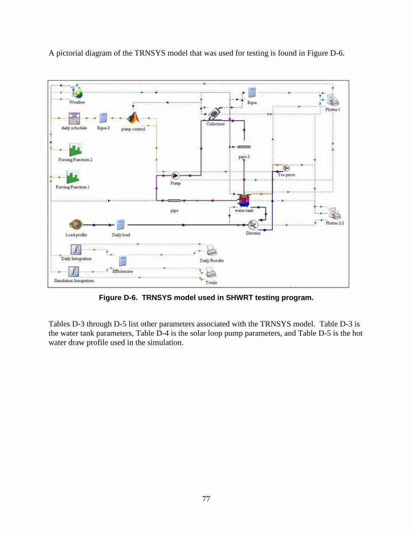
77

A pictorial diagram of the TRNSYS model that was used for testing is found in Figure D-6.

Figure D-6. TRNSYS model used in SHWRT testing program.

Tables D-3 through D-5 list other parameters associated with the TRNSYS model. Table D-3 is the water tank parameters, Table D-4 is the solar loop pump parameters, and Table D-5 is the hot water draw profile used in the simulation.

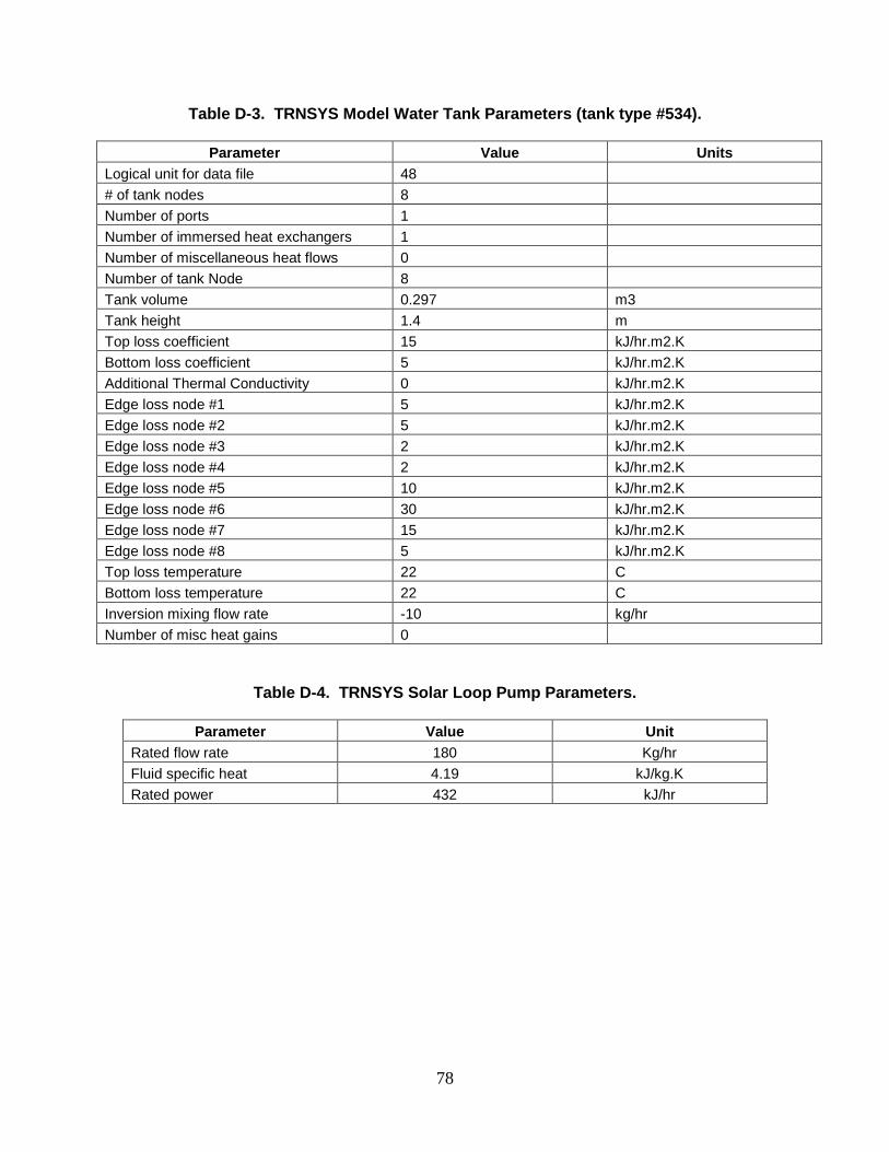
78

Table D-3. TRNSYS Model Water Tank Parameters (tank type #534).

Parameter Value Units Logical unit for data file 48 # of tank nodes 8 Number of ports 1 Number of immersed heat exchangers 1 Number of miscellaneous heat flows 0 Number of tank Node 8 Tank volume 0.297 m3 Tank height 1.4 m Top loss coefficient 15 kJ/hr.m2.K Bottom loss coefficient 5 kJ/hr.m2.K Additional Thermal Conductivity 0 kJ/hr.m2.K Edge loss node #1 5 kJ/hr.m2.K Edge loss node #2 5 kJ/hr.m2.K Edge loss node #3 2 kJ/hr.m2.K Edge loss node #4 2 kJ/hr.m2.K Edge loss node #5 10 kJ/hr.m2.K Edge loss node #6 30 kJ/hr.m2.K Edge loss node #7 15 kJ/hr.m2.K Edge loss node #8 5 kJ/hr.m2.K Top loss temperature 22 C Bottom loss temperature 22 C Inversion mixing flow rate -10 kg/hr Number of misc heat gains 0

Table D-4. TRNSYS Solar Loop Pump Parameters.

Parameter Value Unit Rated flow rate 180 Kg/hr Fluid specific heat 4.19 kJ/kg.K Rated power 432 kJ/hr

79

Table D-5. TRNSYS Hot Water Draw Profile Used in the Simulations.

Hour WattHours 0 150 1 0

2 0 3 0 4 0 5 150 6 900 7 1100 8 900 9 625

10 625 11 430 12 430 13 300 14 180 15 300 16 450 17 450 18 625 19 750 20 625 21 750 22 450 23 300

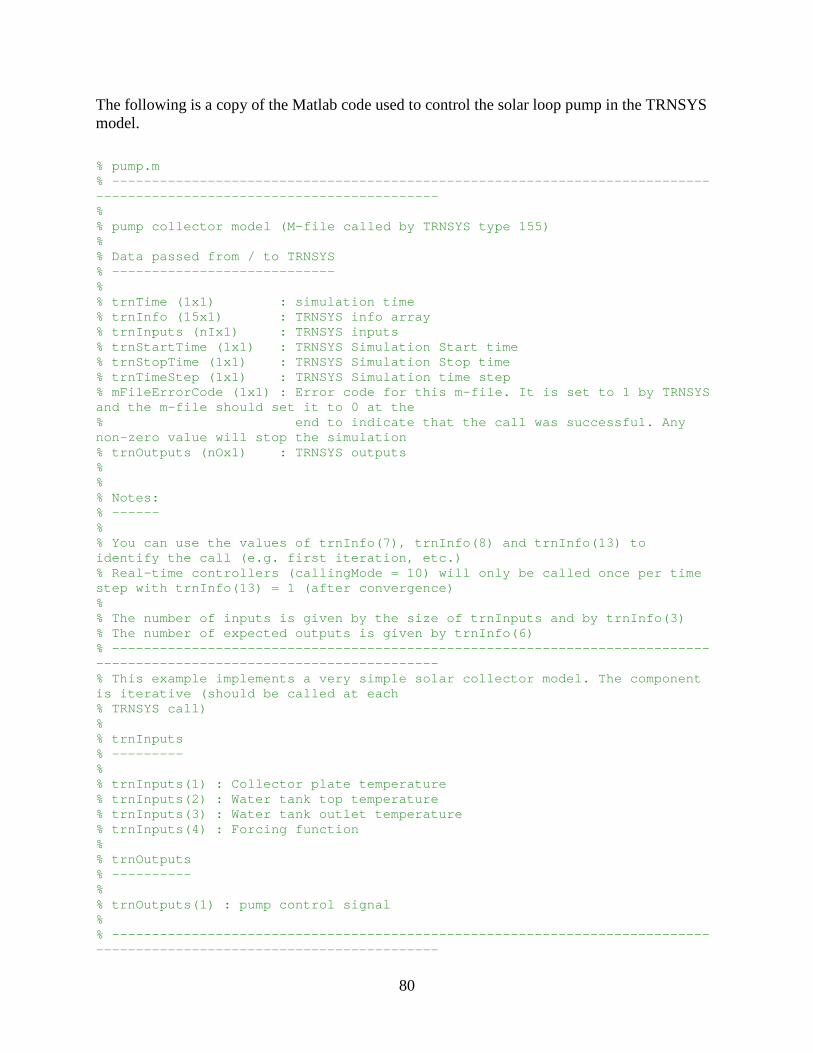
80

The following is a copy of the Matlab code used to control the solar loop pump in the TRNSYS model.

% pump.m % ---------------------------------------------------------------------------------------------------------------------- % % pump collector model (M-file called by TRNSYS type 155) % % Data passed from / to TRNSYS % ---------------------------- % % trnTime (1x1) : simulation time % trnInfo (15x1) : TRNSYS info array % trnInputs (nIx1) : TRNSYS inputs % trnStartTime (1x1) : TRNSYS Simulation Start time % trnStopTime (1x1) : TRNSYS Simulation Stop time % trnTimeStep (1x1) : TRNSYS Simulation time step % mFileErrorCode (1x1) : Error code for this m-file. It is set to 1 by TRNSYS and the m-file should set it to 0 at the % end to indicate that the call was successful. Any non-zero value will stop the simulation % trnOutputs (nOx1) : TRNSYS outputs % % % Notes: % ------ % % You can use the values of trnInfo(7), trnInfo(8) and trnInfo(13) to identify the call (e.g. first iteration, etc.) % Real-time controllers (callingMode = 10) will only be called once per time step with trnInfo(13) = 1 (after convergence) % % The number of inputs is given by the size of trnInputs and by trnInfo(3) % The number of expected outputs is given by trnInfo(6) % ---------------------------------------------------------------------------------------------------------------------- % This example implements a very simple solar collector model. The component is iterative (should be called at each % TRNSYS call) % % trnInputs % --------- % % trnInputs(1) : Collector plate temperature % trnInputs(2) : Water tank top temperature % trnInputs(3) : Water tank outlet temperature % trnInputs(4) : Forcing function % % trnOutputs % ---------- % % trnOutputs(1) : pump control signal % % ----------------------------------------------------------------------------------------------------------------------

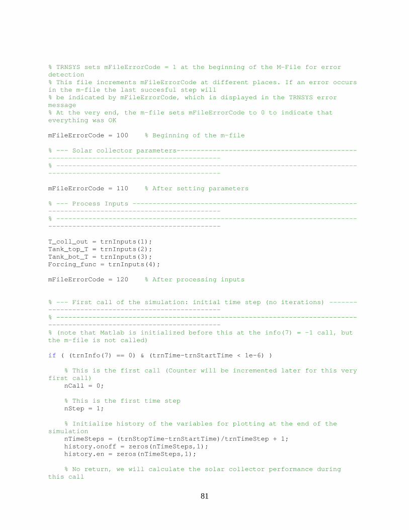
81

% TRNSYS sets mFileErrorCode = 1 at the beginning of the M-File for error detection % This file increments mFileErrorCode at different places. If an error occurs in the m-file the last succesful step will % be indicated by mFileErrorCode, which is displayed in the TRNSYS error message % At the very end, the m-file sets mFileErrorCode to 0 to indicate that everything was OK mFileErrorCode = 100 % Beginning of the m-file % --- Solar collector parameters---------------------------------------------------------------------------------------- % ---------------------------------------------------------------------------------------------------------------------- mFileErrorCode = 110 % After setting parameters % --- Process Inputs --------------------------------------------------------------------------------------------------- % ---------------------------------------------------------------------------------------------------------------------- T_coll_out = trnInputs(1); Tank_top_T = trnInputs(2); Tank_bot_T = trnInputs(3); Forcing_func = trnInputs(4); mFileErrorCode = 120 % After processing inputs % --- First call of the simulation: initial time step (no iterations) -------------------------------------------------- % ---------------------------------------------------------------------------------------------------------------------- % (note that Matlab is initialized before this at the info(7) = -1 call, but the m-file is not called) if ( (trnInfo(7) == 0) & (trnTime-trnStartTime < 1e-6) ) % This is the first call (Counter will be incremented later for this very first call) nCall = 0; % This is the first time step nStep = 1; % Initialize history of the variables for plotting at the end of the simulation nTimeSteps = (trnStopTime-trnStartTime)/trnTimeStep + 1; history.onoff = zeros(nTimeSteps,1); history.en = zeros(nTimeSteps,1); % No return, we will calculate the solar collector performance during this call

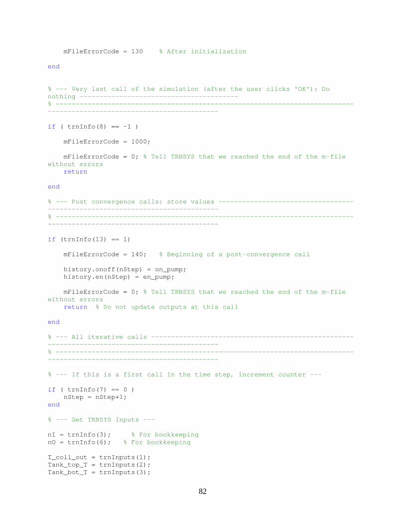
82

mFileErrorCode = 130 % After initialization end % --- Very last call of the simulation (after the user clicks "OK"): Do nothing ---------------------------------------- % ---------------------------------------------------------------------------------------------------------------------- if ( trnInfo(8) == -1 ) mFileErrorCode = 1000; mFileErrorCode = 0; % Tell TRNSYS that we reached the end of the m-file without errors return end % --- Post convergence calls: store values ----------------------------------------------------------------------------- % ---------------------------------------------------------------------------------------------------------------------- if (trnInfo(13) == 1) mFileErrorCode = 140; % Beginning of a post-convergence call history.onoff(nStep) = on_pump; history.en(nStep) = en_pump; mFileErrorCode = 0; % Tell TRNSYS that we reached the end of the m-file without errors return % Do not update outputs at this call end % --- All iterative calls ---------------------------------------------------------------------------------------------- % ---------------------------------------------------------------------------------------------------------------------- % --- If this is a first call in the time step, increment counter --- if ( trnInfo(7) == 0 ) nStep = nStep+1; end % --- Get TRNSYS Inputs --- nI = trnInfo(3); % For bookkeeping nO = trnInfo(6); % For bookkeeping T_coll_out = trnInputs(1); Tank_top_T = trnInputs(2); Tank_bot_T = trnInputs(3);

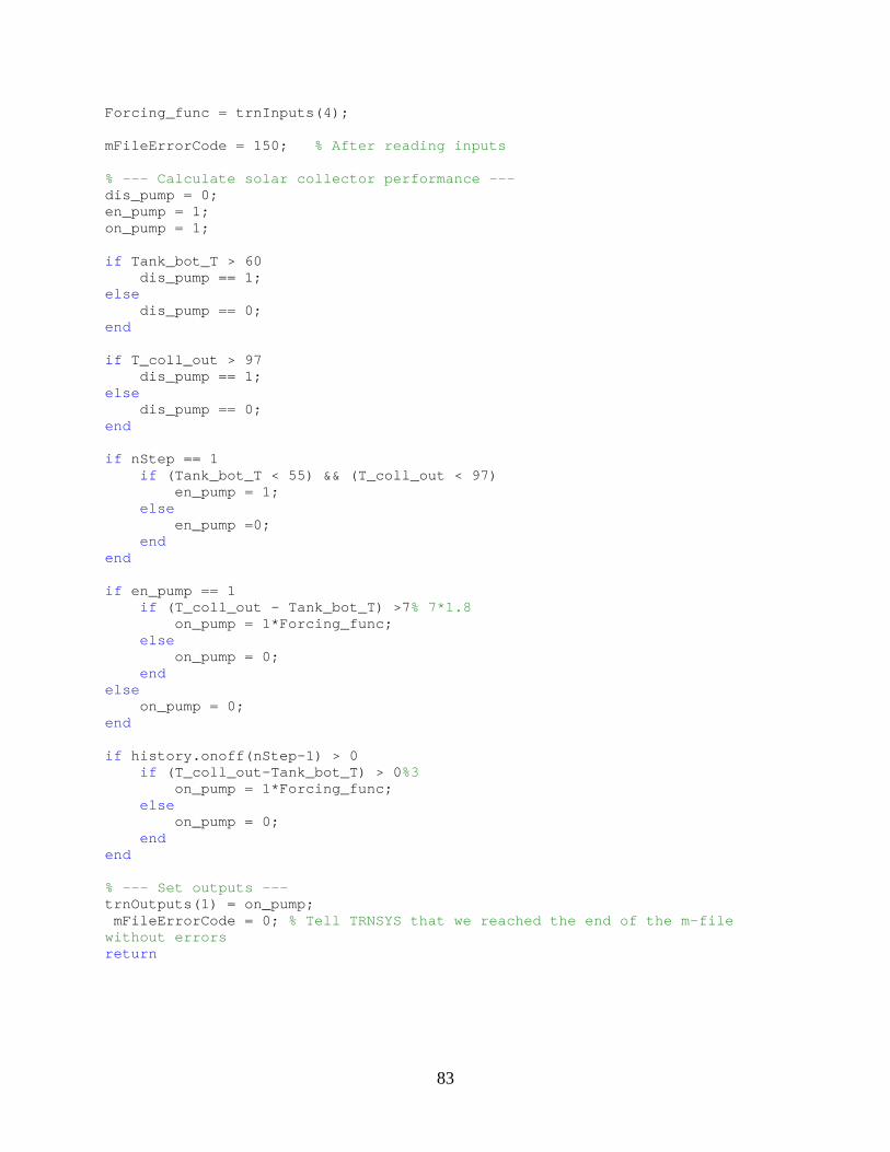
83

Forcing_func = trnInputs(4); mFileErrorCode = 150; % After reading inputs % --- Calculate solar collector performance --- dis_pump = 0; en_pump = 1; on_pump = 1; if Tank_bot_T > 60 dis_pump == 1; else dis_pump == 0; end if T_coll_out > 97 dis_pump == 1; else dis_pump == 0; end if nStep == 1 if (Tank_bot_T < 55) && (T_coll_out < 97) en_pump = 1; else en_pump =0; end end if en_pump == 1 if (T_coll_out - Tank_bot_T) >7% 7*1.8 on_pump = 1*Forcing_func; else on_pump = 0; end else on_pump = 0; end if history.onoff(nStep-1) > 0 if (T_coll_out-Tank_bot_T) > 0%3 on_pump = 1*Forcing_func; else on_pump = 0; end end % --- Set outputs --- trnOutputs(1) = on_pump; mFileErrorCode = 0; % Tell TRNSYS that we reached the end of the m-file without errors return

84

85

Appendix E. Description of the Process for Using TRNSYS Model to Train the ART Algorithms

The following outlines the steps training of the Adaptive Resonance Theory (ART) algorithms using the TRNSYS model.

1. Install TRNSYS Version 16 including the libraries and associated features on a personal computer.

2. Configure the solar hot water (SHW) system model to duplicate as closely as possible the Solar Hot Water Reliability Testbed (SHWRT) system. To the greatest extent possible the components used in the TRNSYS model mirrored the SHWRT system that was used for testing.

3. Verify that the TRNSYS model is accurate by comparing the model predictions with the measured output from the SHWRT. See Appendix C for details.

4. Write hierarchical ART neural networks code in MATLAB. See Appendix E for a copy of the code.

5. Debug hierarchical ART neural networks code. 6. Obtain SOLMET weather data from 1991 to 2005 from National Solar Radiation

Data Base (NSRDB) archives. Remove the parameters of these data that are not used in by the TRNSYS model. Modify the data in this dataset to conform to the requirements of TRNSYS.

7. Run the verified TRNSYS model using data from the database corresponding to years 2000 to 2004. These five years were chosen because they represented the nearest years of data from the current date. Five years were found to be sufficient to train the ART algorithms. In all of the TRNSYS simulation runs the Solar Rating and Certification Corporation (SRCC) load profile was used, the same profile used in the SHWRT testing.

8. Use the simulated outputs from the TRNSYS runs to train the ART algorithms. This process essentially teaches the ART algorithms the normal operation of a SHW system, one that is very similar to the SHWRT.

9. Set aside these trained algorithms for testing against simulated failures based on TRNSYS runs using a weather year that is different from the years used for training.

10. Execute the TRNSYS model for weather 2005 to simulate the failure conditions that would be used to test the ART algorithms. Those failure conditions include a pump failure and a loop flow degradation condition. The reason for using a weather year that was different from the weather years used for training is because a unique set of weather conditions were needed to create a valid test of the ART algorithms.

11. Test the hierarchical ART algorithms using the data that were generated from Step 10. This testing allows various parameters to be evaluated for effectiveness in the ART algorithms as they detect failures. For example, two parameters might be chosen as a starting point: collector plate temperature and water tank outlet temperature. However, after running the test, these set of parameters might be found to be insufficiently robust for use in the ART algorithms in detecting the simulated failures. Based on this information, a different set of parameters might be chosen, ones that are more effective.

86

12. Write ARTMAP neural networks code in MATLAB. This ARTMAP provides a method to identify and label the type of failure associated with various fault conditions.

13. Use the data from the five years of fault-free simulations plus the one year that contained the simulated failures to retrain the ART algorithms.

14. Applied the retrained ART algorithms to the data generated by the SHWRT.

The TRNSYS runs to complete the fault-free runs for years 2000-2004 required about 15 hours of computer time. The computer time required to run TRNSYS for the simulations for the year containing faults, 2005, was about six hours. The required computer time for the training the ART algorithms was about one hour. However, the process of simulating coupled with training required a great deal of human intervention. The intervention is needed to refine the process and ensure that the results are applicable to the upcoming SHWRT tests. Around 400 hours of labor was consumed in the training.

87

Appendix F. Pictures of the Solar Hot Water Reliability Testbed at the University of New Mexico

Figure F-1. Solar Hot Water Reliability Testbed.

Picture of Solar Reliability Testbed

Figure F-3. Front panel of Virtual Instrument for testbed control and instrumentation.

Figure F-4. Partial view of code for the Virtual Instrument.

Figure F-2. Collectors for the testbed (one is covered).

88

89

Appendix G. Functional Specifications for an Advanced Generation Solar Hot Water Controller

An advanced-generation Solar Hot Water controller would have these functional characteristics, capabilities and abilities:

1) Control an SHW in the traditional manner. 2) Monitor energy production performance using solar loop flow and inlet and outlet

temperatures. Display the results on a visual display and record them in storage. 3) Monitor energy production performance using only solar loop flow (not the flow meter)

the patented methods defined in Menicucci et al., U.S. Patent Number 6960017, Non-invasive energy meter for fixed and variable flow systems.

4) Detect faults in the SHW system and announce the fault via one or all of the following: a. Phone call b. Email c. Audible alarm

5) Predict faults in the SHW system by employing self-organizing and self-learning networks and announce the prediction via one or all of the following:

a. Phone call b. Email c. Audible alarm

6) Provide fundamental analysis of the energy performance of the SHW system over various periods of time.

7) Perform “black box” data recording, which upon a failure would store system information just before the failure.

90

91

DISTRIBUTION

1 MS0899 Technical Library 9536 (electronic copy)

92

93