final report - serdp and estcp report.pdfapproach for inferring traits when few data are available....
TRANSCRIPT

FINAL REPORT An Ecoinformatic Approach to Developing Recovery Goals and
Objectives
SERDP Project RC-1475
MARCH 2013
William F. Fagan Maile M. Neel University of Maryland

This report was prepared under contract to the Department of Defense Strategic Environmental Research and Development Program (SERDP). The publication of this report does not indicate endorsement by the Department of Defense, nor should the contents be construed as reflecting the official policy or position of the Department of Defense. Reference herein to any specific commercial product, process, or service by trade name, trademark, manufacturer, or otherwise, does not necessarily constitute or imply its endorsement, recommendation, or favoring by the Department of Defense.

ii
REPORT DOCUMENTATION PAGE Form Approved
OMB No. 0704-0188 Public reporting burden for this collection of information is estimated to average 1 hour per response, including the time for reviewing instructions, searching existing data sources, gathering and maintaining the data needed, and completing and reviewing this collection of information. Send comments regarding this burden estimate or any other aspect of this collection of information, including suggestions for reducing this burden to Department of Defense, Washington Headquarters Services, Directorate for Information Operations and Reports (0704-0188), 1215 Jefferson Davis Highway, Suite 1204, Arlington, VA 22202- 4302. Respondents should be aware that notwithstanding any other provision of law, no person shall be subject to any penalty for failing to comply with a collection of information if it does not display a currently valid OMB control number. PLEASE DO NOT RETURN YOUR FORM TO THE ABOVE ADDRESS. 1. REPORT DATE (DD-MM-YYYY) 15-03-2013
2. REPORT TYPE FINAL
3. DATES COVERED (From - To) 08/04/2006 -- 04/04/2013
4. TITLE AND SUBTITLE RC-1475 An Ecoinformatic Approach to Developing Recovery Goals and Objectives
5a. CONTRACT NUMBER 06-C-0053 5b. GRANT NUMBER
5c. PROGRAM ELEMENT NUMBER 6. AUTHOR(S) Dr. William F. Fagan Dr. Maile Neel
5d. PROJECT NUMBER SERDP RC-1475 5e. TASK NUMBER 5f. WORK UNIT NUMBER
7. PERFORMING ORGANIZATION NAME(S) AND ADDRESS(ES) University of Maryland College Park, MD 20742
8. PERFORMING ORGANIZATION REPORT NUMBER
9. SPONSORING / MONITORING AGENCY NAME(S) AND ADDRESS(ES) SERDP/ESTCP Program 4800 Mark Center Drive, Suite 17D08 Alexandria, VA 22350-3600
10. SPONSOR/MONITOR’S ACRONYM(S) SERDP/ESTCP
11. SPONSOR/MONITOR’S REPORT NUMBER(S) RC-1475
12. DISTRIBUTION / AVAILABILITY STATEMENT Unclassified Unlimited
13. SUPPLEMENTARY NOTES
14. ABSTRACT Lack of data hinders managers’ abilities to set scientifically defensible recovery goals and criteria for all but a few threatened or endangered species. We had twin goals in this project : 1) To develop a suite of database resources that would allow managers to link trait, threat, and recovery data, and 2) to explore patterns in the databases and identify ways of leveraging information across species groups. We used these database resources in several projects focusing on more rigorous establishment of recovery criteria. First, we showed that most recovery criteria are still based on current status and not on species biology. Second we examined the role of PVAs and developed methods to more rigorously estimate population trajectories and critical thresholds for survival when only minimal data are available. Drawing on those methods, we attempted to link traits, threats, and trajectories, but found that species still lacked sufficient data to parameterize models for cross-species comparison. Finally, we implemented a new approach for inferring traits when few data are available. This method uses phylogenetic relationships to fill data gaps in a rigorous way, and was able to accurately predict little “r”, a key trait related to recovery potential in birds and mammals.
15. SUBJECT TERMS Endangered Species; Recovery Goals; Population Growth Rate
16. SECURITY CLASSIFICATION OF: 17. LIMITATION OF ABSTRACT
18. NUMBER OF PAGES
115
19a. NAME OF RESPONSIBLE PERSON William Fagan
a. REPORT UU
b. ABSTRACT UU
c. THIS PAGE UU
19b. TELEPHONE NUMBER (include area code) 301-405-4672
Standard Form 298 (Rev. 8-98) Prescribed by ANSI Std. Z39.18
iii
Table of Contents
List of Figures ............................................................................................................................... vi List of Tables ............................................................................................................................... vii List of Acronyms ......................................................................................................................... vii Keywords .................................................................................................................................... viii Acknowledgements .................................................................................................................... viii Abstract ...........................................................................................................................................1 1. Objectives ...................................................................................................................................3 2. Background ...............................................................................................................................4 3. Part 1: Database Development ................................................................................................7
3.1 – Background .......................................................................................................................7 3.2 – The Recovery Databases ...................................................................................................7
3.2.1 – References from the peer reviewed literature .....................................................10 3.3 – Online search tool ...........................................................................................................13 3.4 – Database resources for data compiled from other resources........................................... 15 3.5 – Summary .........................................................................................................................17
4. Part 2: Understanding Recovery Criteria .............................................................................18
4.1 – Background .....................................................................................................................18 4.2 – Patterns of decline described within recovery plans .......................................................18
4.2.1 – Methods...............................................................................................................19 4.2.2 – Results and Discussion .......................................................................................20
4.3 – How is recovery defined within recovery plans? ............................................................25 4.3.1 – Methods...............................................................................................................25 4.3.2 – Results and Discussion .......................................................................................26 4.3.3 – Conservation-reliant species ...............................................................................32
4.4 – How do biological traits and prior abundances relate to recovery goals? ......................34 4.4.1 – Qualitative delisting criteria for listed plant species with PVAs ........................34 4.4.2 – Predictive approaches to understanding recovery goals .....................................35 4.4.3 – Tree-based methods ............................................................................................35 4.4.4 – Predictive methods for plants ..............................................................................36 4.4.5 – Results and Discussion: Plants............................................................................38 4.4.6 – Results and Discussion: Animals ........................................................................42 4.4.7 – Summary .............................................................................................................44
4.5 – Conclusions .................................................................................................................... 44

iv
5. Part 3: Improving the utility of population viability analysis in recovery planning ........46
5.1 – Background .....................................................................................................................46 5.2 – PVA in ESA recovery planning ......................................................................................49
5.2.1 – Methods...............................................................................................................49 5.2.2 – Results and Discussion .......................................................................................50
5.3 – PVA analysis using time-series data to estimate conservation targets ............................56 5.3.1 – Methods...............................................................................................................57 5.3.2 – Results and Discussion .......................................................................................57
5.4 – Conclusions .................................................................................................................... 59 6. Part 4: Inferring recovery criteria for poorly-studied species ............................................61
6.1 – Background .....................................................................................................................61 6.2 – Comparison sets to infer recovery criteria for species with similar traits and threats ....62
6.2.1 – Time-series approach (Birds) ............................................................................. 65 6.2.2 – Minimal data (plant) approach ............................................................................67 6.2.3 – Summary .............................................................................................................68
6.3 – Testing surrogacy assumptions: Can TES be grouped by traits and abundances? .........69 6.3.1 – Methods...............................................................................................................70 6.3.2 – Analysis...............................................................................................................71 6.3.3 – Results .................................................................................................................71 6.3.4 – Discussion ...........................................................................................................71
6.4 – Conclusions .....................................................................................................................74 7. Part 5: New statistical approaches for the estimation of little “r” .................................... 75
7.1 – Background .....................................................................................................................75 7.2 – A brief history of estimating r ........................................................................................75 7.3 – An examination of the most rigorous estimation methods for r .....................................78
7.3.1 – Methods...............................................................................................................80 7.3.2 – Results and Discussion .......................................................................................81
7.4 – Predicting survivorship curves for use in estimating little r ...........................................84 7.4.1 – Methods...............................................................................................................85 7.4.2 – Results and Discussion .......................................................................................86
7.5 – Conclusion ..................................................................................................................... 88 8. Part 6: Phylogenetic approaches for inferring recovery-related traits for poorly-
studied species ........................................................................................................................89 8.1 – Background .....................................................................................................................89
8.1.1 – General Approach ...............................................................................................89 8.1.2 – Model assessment ...............................................................................................90
8.2 – Mammal implementation: developing the method .........................................................91 8.2.1 – Results and Discussion .......................................................................................97
8.3 – Shorebird implementation ...............................................................................................96 8.3.1 – Results and Discussion .......................................................................................97
8.4 – Conclusions .................................................................................................................. 100

v
9. Conclusions and Implications for Future Research ..........................................................102 9.1 – Further development of phylogenetic approaches ........................................................102 9.2 – Establishing defensible recovery criteria ......................................................................103 9.3 – Future synthetic efforts .................................................................................................104 9.4 – Final Thoughts ..............................................................................................................104
10. Literature Cited ..................................................................................................................105 11. Appendices:
1. Data access ........................................................................................................................116 2. List of scientific/technical publications............................................................................117

vi
List of Figures Figure 1 A conceptual database schema for RecoveryDB and AnimalDB .......................... 8 Figure 2 Home page for RecoveryDB ................................................................................ 14 Figure 3 Query results from RecoveryDB ......................................................................... 15 Figure 4 Proportion of population declines by taxonomic group ....................................... 22 Figure 5 Proportion of range and population losses recorded by state or territory ............ 23 Figure 6 Population levels at different times during the listing process by listing status .. 27 Figure 7 Population levels at different times during the listing process by taxonomic
group .................................................................................................................... 28 Figure 8 Population levels required for delisting ............................................................... 29 Figure 9 Regression tree analysis ....................................................................................... 36 Figure 10 Abundance factors underlying delisting criteria .................................................. 40 Figure 11 Traits underlying delisting criteria ....................................................................... 41 Figure 12 Factors underlying delisting criteria for birds ...................................................... 43 Figure 13 Contexts under which PVA is used or recommended in recovery plans ............. 51 Figure 14 Types of recommended demographic monitoring or research in recovery
plans ..................................................................................................................... 52 Figure 15 Intra-specific variability in PVA results .............................................................. 54 Figure 16 Example quasi-extinction profiles for a species with stochastic population
growth .................................................................................................................. 58 Figure 17 Cross-validation using simulations for three examples of population
structures used to develop the CSEG model ........................................................ 59 Figure 18 Schematic of our original analytical approach ..................................................... 62 Figure 19 Sample ordered proximity graph for a hypothetical species ................................ 63 Figure 20 Hypothetical proximity scores indicating significant and stable comparison
sets ........................................................................................................................ 64 Figure 21 A comparison set of multivariate proximity for Junco hyemalis ......................... 65 Figure 22 Example results from bootstrap randomization tests of the differences between
Junco hyemalis and the nine closest members of its comparison set ................... 66 Figure 23 Number of stable and significant comparison sets for bird species ..................... 67 Figure 24 Number of stable and significant comparison sets for plant species ................... 68 Figure 25 Variable importance values from surrogacy analysis .......................................... 73 Figure 26 Three classic survivorship curves ........................................................................ 76 Figure 27 Using the beta-distribution to model mammalian survivorship ........................... 82 Figure 28 Map of the influence of survivorship shape on estimate of r .............................. 83 Figure 29 Histograms of empirical estimates of the different measures of r ....................... 84 Figure 30 Survivorship curve parameters displayed in shape space .................................... 86 Figure 31 Comparison of survivorship shapes from wild and captive populations ............. 87 Figure 32 Relationship between observed and predicted r .................................................. 92 Figure 33 Histograms of prediction error for observed r values .......................................... 93
vii
Figure 34 Predicted and observed r values ..........................................................................94 Figure 35 Phylogenetic relationships and observed and predicted values of r ....................95 Figure 36 Histograms of prediction error for observed r values for birds ...........................97 Figure 37 Predicted and observed r values for birds ............................................................98 Figure 38 Phylogenetic relationships and observed and predicted values of r for birds ......99
List of Tables Table 1a Attribute fields for RecoveryDB and AnimalDB ................................................11 Table 1b Attribute fields for life history databases .............................................................16 Table 2 Qualitative data for declines ................................................................................21 Table 3 Decline pattern by taxonomic group ....................................................................22 Table 4 Summary of conservation-reliant status ...............................................................33 Table 5 Qualitative delisting criteria in plant recovery plans with PVAs .........................35 Table 6 Summary of abundances and delisting criteria from recovery plans ...................37 Table 7 Predictor distribution and biological traits ...........................................................38 Table 8 Results from 28 model runs .................................................................................39 Table 9 Characteristics of a reliable, robust PVA .............................................................47 Table 10 Characteristics of plant PVAs in the published literature ....................................53 Table 11 Summary of abundance variables included in surrogacy analyses ......................70 Table 12 Summary of random forest analysis linking traits, threats, and abundances .......72 Table 13 Different measures of population growth rate .....................................................79
List of Acronyms AnimalDB Animal Recovery Database cRF Conditional Random Forest cTREE Conditional Tree CSEG Corrupted Stochastic Growth Model DA Diffusion Approximations DOD Department of Defense ESA Endangered Species Act MVP Minimum Viable Population NMFS National Marine Fisheries Service PCA Principal Components Analysis PIC Phylogenetic Independent Contrasts PVA Population Viability Analysis RecoveryDB Plant Recovery Database RF Random Forest TES Threatened and Endangered Species TESS Threatened and Endangered Species Database USFWS United States Fish and Wildlife Service WSS Well-studied Species

viii
Keywords Corrupted Stochastic Exponential Growth model; Endangered Species; ESA Listed Species; Euler equation; Intrinsic Rate of Increase; Life History Traits; Population Growth Rate; Population Viability Analysis; r; Recovery Goals; Recovery Criteria; Survivorship; Threatened Species
Acknowledgements Funding for this work was provided by the Strategic Environmental Research and Development Program (SERDP). We gratefully acknowledge the many comments, suggestions, and helpful criticisms that Drs. Debby Crouse and Heather Bell of the US Fish and Wildlife Service made over the course of this project. We further acknowledge the essential efforts made to the project by the many postdoctoral researchers we were able to support in whole or in part over the course of the award, including Drs. Sharon A Bewick, Lesley G Campbell, Judy P Che- Castaldo, Emma Goldberg, Joanna Grand, Allison K Leidner, David A Luther, Yanthe Pearson, Leslie Ries, and Sara L Zeigler. These scholars played critical roles in many aspects of the project including leading aspects of data development and analyses. Several graduate students made critical contributions to the effort through data analyses, visualization, and data development, including Paula V Casanovas, Elise A Larsen, Eric M Lind, and Jessica B Turner. We are also grateful to the many undergraduates would made helpful contributions to the project, through development of the databases and in other ways, including Anthony M Accetta, Nikolaus G Anderson, Adam L Bazinet, Jennifer L Billiet, Robert K Burnett, Raymond W Chow, Laurel A Eckstrand, Steven J Goldstein, Piyali Kundu, Manasee P Mahajan, Louis Marti, Amy E Norris, Liliana Orellana, James Pettengill, Tara M Ruoff, Anna C Schoenfelder, Hilary A Staver, Brittany E West, and Caroline J Wick.
1
Abstract
Objectives - A profound lack of data hinders managers’ abilities to set scientifically defensible recovery goals and criteria for all but a few species that are listed as threatened or endangered under the Endangered Species Act. Given such data gaps, managers tend to jump between generic conservation rules and expensive, time-consuming, and often unattainable single-species PVAs. Our goal was to develop an analytical framework that would take advantage of shared traits and threats across many species to develop a pathway towards a more defensible system of developing recovery criteria. To do this, we developed multiple database resources containing compiled information on species recovery data, population trajectories, and life-history traits.
We had twin objectives in undertaking an informatics approach to conservation. The first was to develop an analytical framework for inferring critical conservation information based on shared threats and traits. The second was to develop a resource that managers and agencies could use to make better conservation decisions, possibly following analytical frameworks or using the data in ways that we did not consider. We were able to use the database resources we developed to make some major breakthroughs in understanding the linkages between species biology, conservation potential, and recovery criteria. However, our experience was that there still are not enough species-specific data to allow robust cross-species modeling. In adjusting to this reality, we adapted our objectives to include 1) developing database resources to enhance conservation management, 2) understand key patterns in recovery criteria, 3) improve the utility of Population Viability Analysis (PVA), 4) determine the potential to infer recovery criteria for poorly studied species, and 5) develop new approaches for inferring traits for poorly studied species.
Technical Approach - Our technical approach for achieving our objectives was to build a series of databases from the literature and recovery plans, and then use those data to carry out novel analyses. The largest resource is a set of databases of information from 288 recovery plans for 642 plants and ~400 plans for 528 animal species. We extracted information on every aspect of listing and conservation status, habitat requirements, and from over one hundred traits of biological importance. In addition, we compiled resources on well-studied species, especially plants, birds, and mammals and have made those resources available as well. We used these databases to carry out analyses on patterns in recovery criteria, patterns in PVAs, the ability to model recovery criteria based on traits, and the ability to infer traits using phylogenetic approaches.
Results - We undertook a full examination of different aspects of recovery, including how it is defined, and how recovery criteria are linked to patterns of decline and species’ biology. Overall, despite years of criticism, recovery criteria continue to be defined more by the current status of the species (e.g., the species’ listing status and population levels) than by the specifics of their biology or individual needs. This disappointing fact means suggests minimal opportunities to link current recovery criteria with biological traits under an analytical framework.
In realizing that most plans lacked quantitative data to support recovery criteria, we closely examined one of the primary methods used to support recovery criteria, PVA. PVA is still considered by some scientists to be the “gold standard” in establishing defensible recovery goals. However, PVAs have also been criticized because uncertainty inherent in the modeling process may make it an inappropriate tool for assessing absolute outcomes or prescribing

2
absolute population sizes. Our study revealed that PVAs have seen very limited use in recovery plans. PVAs have only been used to help determine delisting criteria for five listed plant species and are included in the description for only nine listed species. Furthermore, despite a long history of criticism and suggestions to improve rigor, most PVAs, as carried out, fail to meet minimum standards for use in recovery planning.
As an alternative to data-hungry mechanistic PVAs, we present a statistical approach for extracting parameters from time-series data that are relevant to the establishment of recovery criteria. The approach is based on the idea that certain average properties of stochastic processes may be predictable even when the details of the underlying process are unpredictable and/or unknown. Our goal was to extend this type of reasoning to the estimation of a specific property of stochastic population trajectories: the probability of decline below a pre-defined threshold (i.e., quasi-extinction). We successfully used this model to output quasi- extinction probabilities for a broad class of population change processes.
Because we could not find a rigorous link between traits and published recovery criteria, we next used the procedures developed in our quasi-extinction model to explicitly link species traits, threats, and population trends (instead of recovery criteria). However, our attempt to build sets of similar species was unsuccessful. We were never able to produce enough stable and significant comparison sets to proceed with the inverse modeling efforts that we had planned. Considering our focus was on relatively well-studied taxa (plants and birds), this does not bode well for applying the method broadly at this point. Yet even exploring simpler surrogacy approaches proved elusive. Based on these disappointing results, we realized that we needed to find a new approach for leveraging the information we have about species in way that would usefully inform their recovery. We decided to switch to evolutionary statistical models and focus our attention on predicting species maximum population growth rates, a fundamental metric in population biology known as “little r” or r , the intrinsic rate of increase.
Very generally, r describes trends in population density and abundance and is an indication of the potential for a population to replace itself. As a fundamental life history trait, r integrates how long a species lives, patterns in death over the course of a typical lifetime (referred to as survivorship curves), and lifetime reproductive capacity into a single metric. We present advancements made in estimating r and we also show how r is more strongly related to taxonomic ancestry than it is to body mass, as is typically believed. The realization that r had a strong phylogenetic signal led us to develop a model that could predict r based on shared traits, phylogenetic structure, and knowing the value of r for a subset of species in each clade. We showed that this method was successful for birds and mammals. Benefits - In the course of this project, we have developed four substantial databases that have been released to the public. We have also carried out a series of analyses showing the limitations of the current “state-of-the-art” approaches to conservation science. These limitations have two causes, still too-sparse data and also that generalizations between species are still elusive. However, we have provided two new analytical techniques that could have widespread value to the conservation community, both in and outside of federal lands. The first is a new method of producing key parameters from PVAs without detailed process data and the second is a novel phylogenetic approach to estimating key life-history parameters for species where we continue to have a paucity of data.

3
1. Objectives
We had two complementary sets of objectives for this project. Each was related to the goal of enabling the DOD to do a better job of meeting its requirements for management for threatened and endangered species, especially for species where little information is available to support action. The first set of objectives was to develop a database that compiled information available for two broadly-defined sets of species. The first group was any species listed by the US Fish and Wildlife Service (USFWS) as either threatened or endangered species (abbreviated here as TES) that for which there was an approved recovery plan. The second group was any well-studied species (WSS) that had either a population viability analysis or time series data available. Our goals for these databases were to compile the following information:
1. threats; 2. life history or trait information that would allow us to generalize patterns from
one species group to another; and 3. population levels through time 4. established recovery criteria.
The second set of objectives focuses on using the data compiled above to understand the nature of listed species, and to use the information about traits, threats, and abundances to develop a suite of models that could support development of recovery criteria when data are limited. To do this, we carried out research that allows us to:
1. understand the scientific defensibility of listing goals and recovery criteria in recovery plans;
2. evaluate the use of population viability analysis for recovery planning; 3. determine if recovery goals or recovery potential can be inferred from well to
poorly studied species; and 4. develop methods for inferring unknown traits using information from well-studied
species.

4
2. BACKGROUND The Endangered Species Act of 1973 (ESA) establishes a visionary commitment to protecting biodiversity in the United States using the best available science. The primary goals of the ESA, which is implemented by the U.S. Fish and Wildlife Service (USFWS) and the National Marine Fisheries Service (NMFS), are to prevent extinction and to recover species such that they are no longer in need of the ESA’s provisions for survival. Recovery is achieved through development and implementation of recovery plans that specify scientifically-based, measurable, objective recovery criteria (e.g., numbers of populations or population sizes) as well as management actions that ameliorate threats such that the species can be downlisted or delisted. However, recovery plans for many species do not establish such criteria (Gerber and Hatch 2002), and, when they do, criteria have been criticized for being unrelated to inherent biological characteristics (Clark et al. 2002; Elphick et al. 2001; Gerber and Hatch 2002) or too low to adequately protect populations into the future (Tear et al. 1993, 1995). The more than 350 listed species on Department of Defense (DoD) lands result in significant conservation and recovery responsibilities which often include land set-asides and limitations on military training opportunities. Our goal for this project was to develop an approach that could increase the scientific defensibility of recovery criteria that could be used even in absence of extensive data for most species.
Several major reviews of recovery had been completed in the mid-1990’s. These reviews were based on recovery plans approved before 1992, at which time the number of species with plans represented only a small fraction of the species that currently have plans. Overall, Tear et al (1995) reported that often species tended to be listed only after they were too endangered to have high likelihood of recovery (i.e., recovery could be achieved for 37% of 163 species). They also concluded that abundances required for delisting species that did have recovery potential would leave most species far too vulnerable to extinction. For most species, recovery plans indicated that delisting would be allowed with no more populations than existed at plan writing, that biological information was lacking for most species, and that recovery criteria focused more on individual and population abundances than amounts of habitat and range. A subsequent analysis by Elphick et al. (2001) questioned the biological basis of delisting criteria for 27 bird species because they found that the numbers of individuals required for delisting were best predicted by the numbers of individuals at plan writing, rather than by body mass, fecundity, or lifespan.
The requirement for objective and measurable recovery criteria in the 1988 amendment to the Endangered Species Act (ESA) spurred development of conservation methods that provide objective, measurable, species-specific recommendations. Population viability analysis (PVA) has been strongly advocated to determine the "minimum viable population" (MVP), or the population size needed for persistence over a given time period. Some scientists consider PVA to be valuable for defining recovery objectives because this type of model links underlying biological mechanisms with observed population trends and thus can be used as a tool for making predictions or setting specific conservation targets (Morris and Doak 2003). The most common type of PVA approach is to build a mechanistic model that accounts for each biological stage involved in births, deaths, immigration and emigration and then parameterize the model with data relevant to each stage, including transition probabilities. Such high-quality data are rarely available to conservationists (Morris et al. 2002, DeMaster et al. 2004). Furthermore, even when expensive data-collection efforts are possible, PVA results likely do not apply to

5
other species or even other localities or future conditions for the same species (Flather et al. 2011).
A second population modeling approach has been to use time-series abundance data (a data type that is much more widely available) to track population processes and use them to infer underlying dynamics. Yet, to date, these approaches have not produced specific conservation targets, only predictions of future population trajectories under the assumption that conditions remain the same. Although data requirements for time series analyses are lower than for traditional PVA approaches, they are still more intensive than can be supported for most species. Further, issues of applicability beyond the sampled populations remain. Absence of data for PVA or time series analysis of abundance data creates a critical need for alternative approaches to determining scientifically defensible recovery criteria specific to each listed species. At the other end of the spectrum, when few or no data are available, broad rules of thumb have been developed that don’t necessarily require detailed species-specific information. These general rules of thumb are supported by basic theory and conservation principles and are applied to poorly known species. These rules may provide some useful management guidelines within groups, but may be inadequate when applied across a broad range of taxa with widely varying life histories and ecological characteristics. For example, it is well known that the population size needed to conserve an endangered insect is vastly greater than the population size needed to conserve a bear or similar species. However, these approaches are rarely applied in such a broad-brush fashion. Their application is problematic when going from general principles to specific abundance levels because it will be difficult or impossible to defend those abundances as being both necessary and sufficient. This dichotomy between lack of data for species specific recommendations and broad rules of thumb is especially problematic for land managers that have to balance multiple uses such as the DoD, whose main goal is advancing mission readiness.
One of the most attractive approaches to finding a middle way through the problem of lack of data is to link species biological traits with the threats they face, and then build from that linkage to develop broadly defensible recovery criteria. This approach is attractive because so much of ecological and evolutionary theory is grounded on the idea that species-level traits matter for population dynamics, species interactions, and ecosystem function. For example, the metabolic theory of ecology holds that a species body mass is central to understanding a host of biological processes at multiple levels of organization (Brown et al. 2004). Overall, more than 3000 scientific articles have been written about some aspect of the linkage between species-level life history traits and conservation. This intensity of effort suggests that there is a natural inclination within the research community to think of traits as a source of insight into conservation success. Put another way, it is conceptually appealing that there should be some fundamental principles at work, that once identified, would facilitate development and organization of guidelines for conservation efforts based on underlying species-level traits.
Our goals for this project were to develop an approach for defining recovery that capitalized on application of data from well-known species to situations where few data are available. To do this, we developed two databases (one for plants and one for animals) that contained information extracted from all recovery plans that had been written by 1 January 2010. The development, content, and use of those databases are described in Part 1 of this report. We drew on those databases to achieve several goals. The first was simply to better understand the patterns of recovery criteria and the associated information in the recovery plans. Those patterns are reported in Part 2 of this report. Next, by bringing in additional information from the published literature and from other database sources, we continued to examine the potential for

6
PVA to be a tool for developing scientifically defensible recovery criteria by continuing to develop methods when only time-series abundance data are available, but also to understand how PVAs are used currently, and determine if those uses conform to current best practices. Those results are described in Part 3 of this report. The next two sections describe our progress in developing methods for recovery when data are lacking. Part 4 describes attempts to model recovery criteria based on shared traits, threats, and population trajectories.
These attempts highlighted the reality that currently available data remain insufficient to make broad inferences about recovery criteria across diverse species. Furthermore, in many cases, what inferences one can make can hinge upon which pieces of data are available and for what species. This means that the ‘lack of data’ problem constitutes the foremost hurdle to cross-species inferences, and such inference are likely to always remain difficult and, even in the best of circumstances, to hinge upon detailed statistical analysis. More importantly our results are indicating that the application of the surrogate species concept for estimating recovery criteria is fundamentally flawed even when data are more readily available. Given this vexing problem concerning the lack of sufficient species-specific information, we adopted an evolutionary perspective, and sought to use species’ shared evolutionary history to advantage in filling in missing data. We implemented this method by focusing on one critical trait, the maximum rate of population growth (also called “little r” or the intrinsic rate of population increase, and denoted by r) . This species-level parameter describes a species’ capacity for population growth. This measure can be calculated from a species’ biological traits, and sets an upper limit on its performance in the face of external threats. Consequently, this measure is an important trait for understanding a species’ conservation potential. As we researched this path, we found that it was first necessary to develop, implement, and compare a series of statistical approaches for estimating r and for characterizing the relationship between r and other traits, such as body mass, and all of these efforts are described in Part 5. In Part 6, we present a method for estimating little “r” based on phylogenetic relationships and show it is indeed possible use this approach to make reasonable estimates for r when no species-specific data are available. We end this report with a synthesis of our efforts and a roadmap for future work because the need for developing tractable, yet defensible, species recovery criteria remains as important as ever.

7
3. PART 1: DATABASE DEVELOPMENT 3.1 - Background We had three main goals in developing a suite of database resources. The first was to compile the data necessary to do the analyses that were at the core of this project. The second was to determine how much data were available for the types of cross-species analyses that we proposed. Third, the data collected as part of this project will be made public so that others can take advantage of these resources.
Throughout the course of this project, we have compiled information from several sources and for targets. The first major part of this effort was to extract information directly from all approved recovery plans for federally listed plants and animals. This information was extracted and put into one database for plants (hereafter, RecoveryDB) and one database for animals (hereafter, AnimalDB). The databases were kept separate because different types of biological information are relevant for plants versus animals. In addition to the information extracted from recovery plans, RecoveryDB also includes a list of peer-reviewed publications prior to 2010 that have data relevant to the listed species (although the trait data themselves are not in RecoveryDB). These publications did not necessarily contain trait information but rather were gathered to understand what scientific information was available in the published literature. We also sought to compile information on well-studied species which we defined as those species having population viability, time series abundance data, or quantitative data on demographic parameters related to population growth. For those species we also scoured the literature for the same life history and other biological traits that we collected for the listed species so that we could model minimum viable population estimates for these species with biologically similar listed species. 3.2 - The Recovery Databases We have developed two, separately implemented on-line resources for data coming from approved recovery plans, one for plants (RecoveryDB) and one for animals (AnimalDB). Although there are some differences in specific attributes, the structure and implementation of both databases is largely the same. Therefore, we describe the basics of structure and database implementation for both, but highlight differences for each throughout.
RecoveryDB and AnimalDB are PostgreSQL databases and the query interface structure is implemented with PHP. The databases are served from a Linux-based server housed by the Office of Information Technology for the Department of Plant Science and Landscape Architecture. Both of these databases are available to be viewed online and access information is given in Appendix 1. Several different classes of information were extracted from each recovery plan, and the basic links between different types of data are shown in a conceptualized schema in Fig. 1. Note that although the schema represents both plants and animals, the databases are completely separate and implemented on separate Web pages (see below). The databases organize information from two major types of sources. The first are the approved recovery plans. Each species is represented in a table of species and that table is linked to tables for the recovery plans and for attributes of each species. Species were organized in taxonomic groups so information can be organized by taxonomic group if necessary. The table of attributes
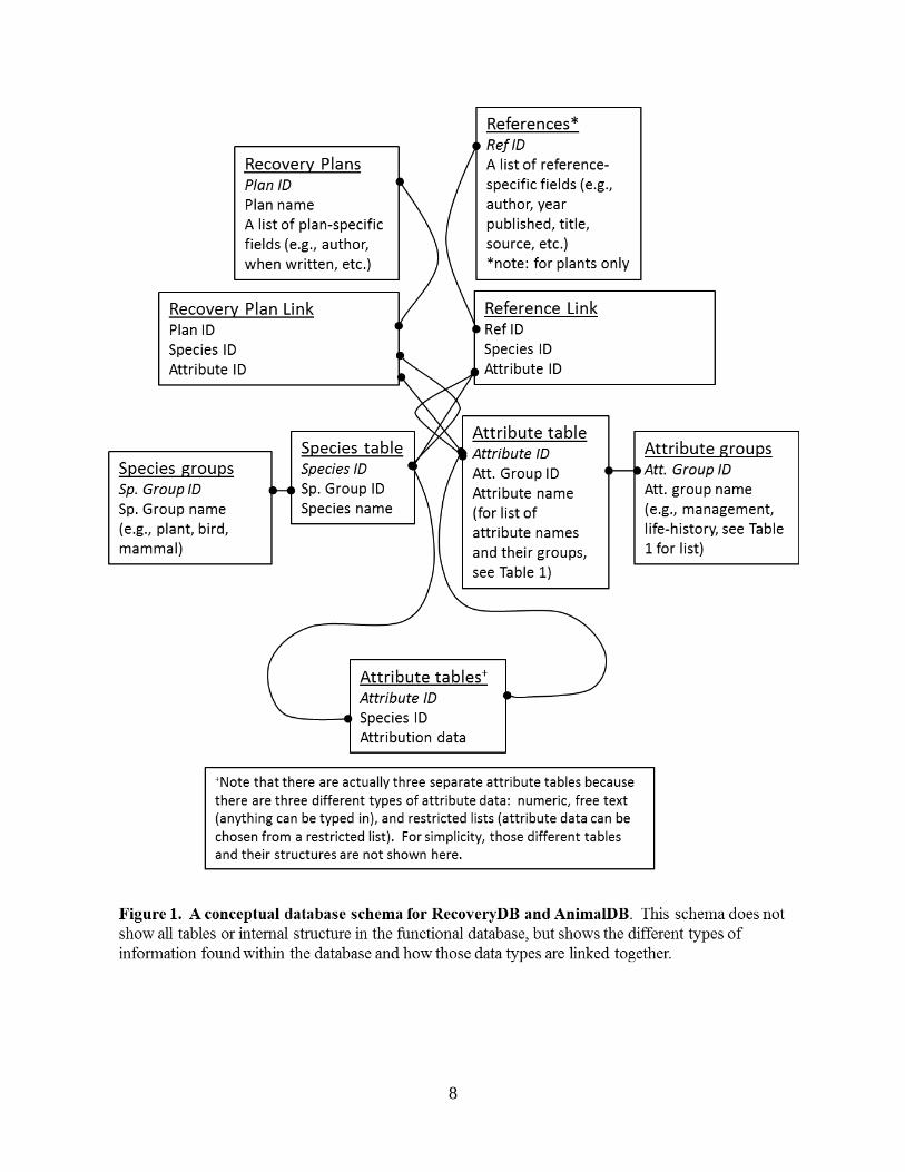
8

9
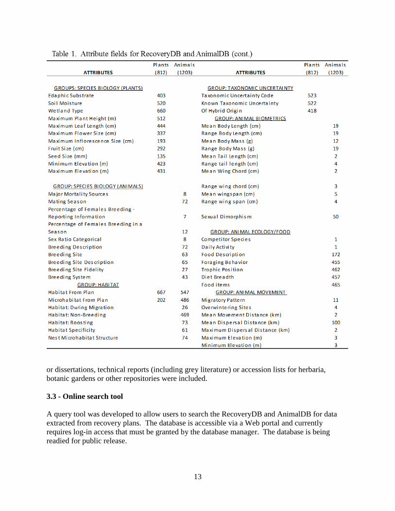
that include data for each species to contain information extracted from each recovery plan was developed. A total of 169 attributes were identified for plants and 243 for animals; with some overlapping fields. For each recovery plan, information about each attribute was extracted and entered into the attribute tables as available.
All plant TES with an approved recovery plan published as of January 1, 2010 were included in the database regardless of whether they are located on DoD or DoE lands. For quantitative abundance values, multiple observers collected data independently and these data were then compared and reconciled to ensure quality control. Sometimes differences were due to simple human error, but more often they were due to different interpretations on the part of the two observers. Reconciling these abundances was an arduous process that involved extensive effort. Additional quality checking of values was achieved through checking outliers during data summary efforts. Qualitative data were quality controlled first through limiting the potential entry to pre-established lists. Such lists limit errors due to typographical errors or subtle differences in wording. Second we built in automatic dependencies for hierarchical relationships such that if a lower level attribute was true for a species, all higher levels were automatically true. Values of each attribute were also checked after entry for logical consistency across species. Data proofing and quality checks are a major undertaking for a project this size and efforts at error reduction and elimination are ongoing. All data used in analysis to date have been cross-checked multiple times by 2-3 observers. Data were entered from all recovery plans for available for the 812 plant and 1203 animal listed as recovery entities, hereafter referred to generically as species. After data extraction was complete, not all attribute fields ended up being used and there was a tremendous amount of variability in data availability from plan to plan. Table 1 shows all the fields that had data entered into them, and how many species had data entered for each field type. Note that attributes are grouped into general categories and some are plant or animal-specific (Table 1). Verifying the underlying quality of the data presented in the recovery plans was beyond the scope of our data collection efforts. In particular, confirming or investigating cause and effect relationships between identified threats and declines in each species was far outside the scope of our project. We handled threats in two ways. First, we recorded the threats as identified in the plans (e.g., development, agriculture, off-highway vehicle use, invasive species, etc.) as well as the ultimate manifestation of those threats (reduction in numbers of individuals, numbers of populations, or range extent). The basic threats as we first collected them were not directly usable because they were not presented consistently in plans and for our purposes under this project the ultimate manifestation were more relevant. Thus, all analyses to date have used threats expressed as the ultimate manifestation. Examples of inconsistencies are that one plan might list agriculture as a threat whereas others might specify the type of agriculture; one plan might specify ‘transportation’ (which could include road construction or maintenance, railroads, shipping, etc.) whereas others might specify the aspect of transportation (e.g county road maintenance). We are continuing to improve the basic threat data by working with USFWS to apply a classification system they are adopting that will allow us to put threats into a useful hierarchy and to separate out stressors from the consequences of those stressors. We will ultimately explore the relationship between identified threats and recovery strategies, but such exploration is beyond the analysis needed for this project. Much of the continuing work on threats is being led by Dr. Judy Che-Castaldo through a postdoctoral fellowship at the SocioEnvironmental Synthesis Center (see Conclusions).

10
3.2.1 - References from the peer-reviewed literature A great deal of information has been culled from the peer-reviewed literature to compile database resources for well-studied plants and animals that have been the focus of scientific research (see Well-studied database section below). For plants, the references with data for each of the 169 attribute fields were also compiled into a table and included in the RecoveryDB online implementation (Fig. 1). This table allows users to query for which species have any of the 169 types of information published and for users to obtain a list of those references published up until 2010 that have information relevant to each of the fields.
For RecoveryDB itself, only references from the peer-reviewed literature were included in these reference links. No information from abstracts, floras, manuals, field guides, or theses were included. These reference sources were used, however for compilation of information for well-studied species that did not have recovery plans.

11

12
13
or dissertations, technical reports (including grey literature) or accession lists for herbaria, botanic gardens or other repositories were included. 3.3 - Online search tool A query tool was developed to allow users to search the RecoveryDB and AnimalDB for data extracted from recovery plans. The database is accessible via a Web portal and currently requires log-in access that must be granted by the database manager. The database is being readied for public release.

14
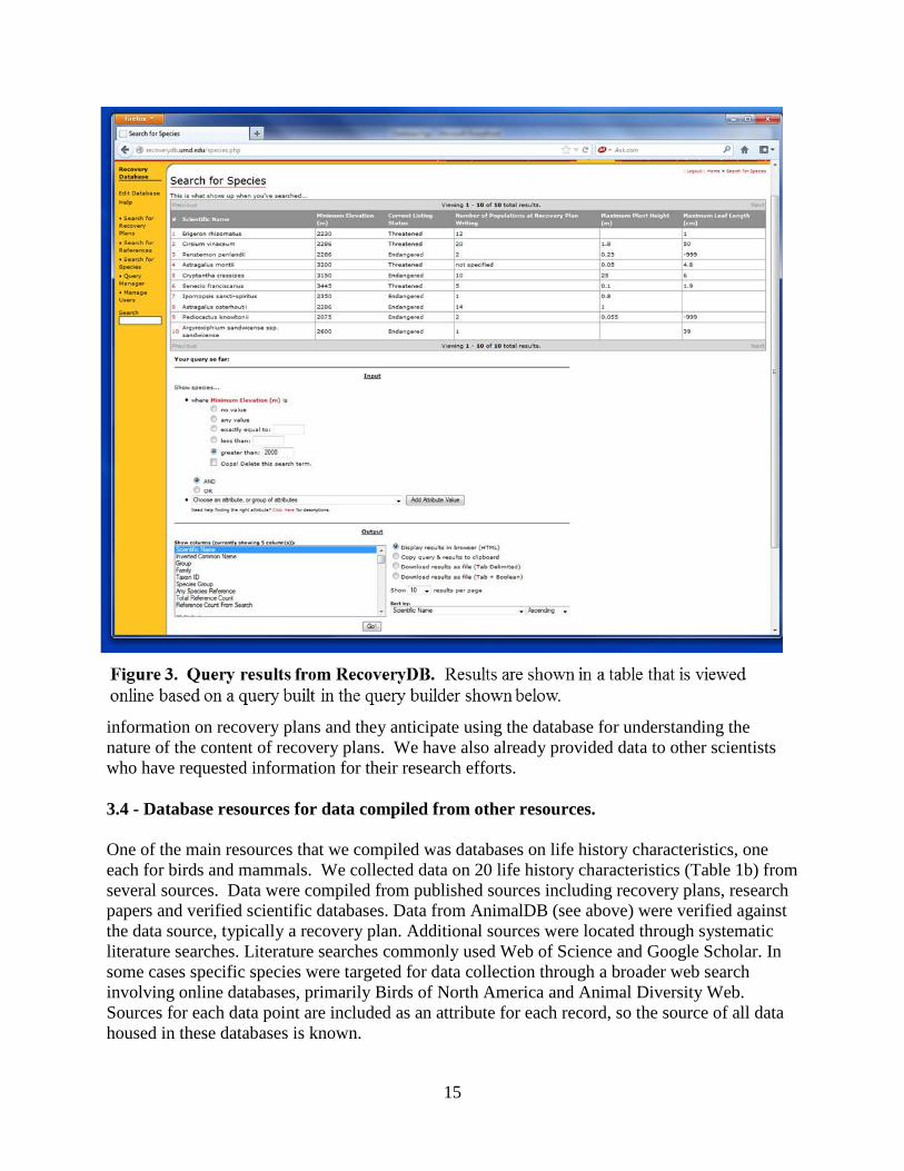
The home pages for RecoveryDB and AnimalDB give access to all the features of the database (home page for RecoveryDB shown in Fig. 2). There are three query tools that allow users to access information based on species attributes (Species query), based on information in the recovery plans (Recovery plan query), and (for plants only), reference search from the peer reviewed literature (Reference query). Note that public users will not be able to see the “edit database” tab (Fig. 2); this will only be available to users with administrative permissions. Instructions on keeping the database updated are shown in Appendix 1.
All three query tools are similar in construction. We show the results of one query where we searched the database for all plants whose minimum elevation is greater than 2000m. For each plant that met those requirements, we asked to view minimum elevation (m), current listing status, number of populations at recovery plan writing, maximum plant height (m) and minimum leaf length (cm). Results for 10 species were returned into a table (upper part of Fig. 3) and the query interface can be seen below (Fig. 3). There is also a query manager that allows users to save queries that they use frequently (Fig. 2).
This data will be made accessible and the main value of the database will be to researchers and agency personnel with broad questions about patterns in endangered species and their recovery. One of the main groups that we have worked with to build a database useful for agencies to be able to make better decisions is the USFWS. We have been in close contact with them to ensure that the data are useful. We have regularly responded to their queries for
15
information on recovery plans and they anticipate using the database for understanding the nature of the content of recovery plans. We have also already provided data to other scientists who have requested information for their research efforts. 3.4 - Database resources for data compiled from other resources. One of the main resources that we compiled was databases on life history characteristics, one each for birds and mammals. We collected data on 20 life history characteristics (Table 1b) from several sources. Data were compiled from published sources including recovery plans, research papers and verified scientific databases. Data from AnimalDB (see above) were verified against the data source, typically a recovery plan. Additional sources were located through systematic literature searches. Literature searches commonly used Web of Science and Google Scholar. In some cases specific species were targeted for data collection through a broader web search involving online databases, primarily Birds of North America and Animal Diversity Web. Sources for each data point are included as an attribute for each record, so the source of all data housed in these databases is known.
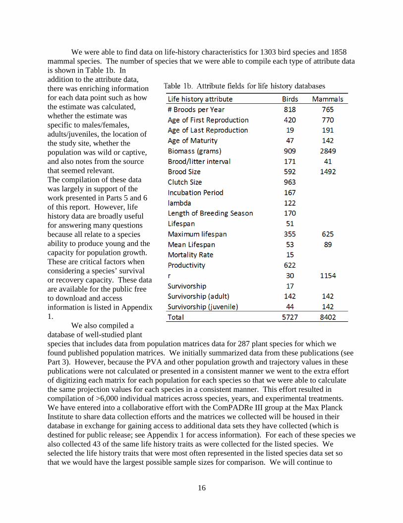
16
We were able to find data on life-history characteristics for 1303 bird species and 1858 mammal species. The number of species that we were able to compile each type of attribute data is shown in Table 1b. In addition to the attribute data, there was enriching information for each data point such as how the estimate was calculated, whether the estimate was specific to males/females, adults/juveniles, the location of the study site, whether the population was wild or captive, and also notes from the source that seemed relevant. The compilation of these data was largely in support of the work presented in Parts 5 and 6 of this report. However, life history data are broadly useful for answering many questions because all relate to a species ability to produce young and the capacity for population growth. These are critical factors when considering a species’ survival or recovery capacity. These data are available for the public free to download and access information is listed in Appendix 1.
We also compiled a database of well-studied plant species that includes data from population matrices data for 287 plant species for which we found published population matrices. We initially summarized data from these publications (see Part 3). However, because the PVA and other population growth and trajectory values in these publications were not calculated or presented in a consistent manner we went to the extra effort of digitizing each matrix for each population for each species so that we were able to calculate the same projection values for each species in a consistent manner. This effort resulted in compilation of >6,000 individual matrices across species, years, and experimental treatments. We have entered into a collaborative effort with the ComPADRe III group at the Max Planck Institute to share data collection efforts and the matrices we collected will be housed in their database in exchange for gaining access to additional data sets they have collected (which is destined for public release; see Appendix 1 for access information). For each of these species we also collected 43 of the same life history traits as were collected for the listed species. We selected the life history traits that were most often represented in the listed species data set so that we would have the largest possible sample sizes for comparison. We will continue to

17
analyze these data, but their collection took much longer than anticipated is just coming to completion. Additional resources for well-studied animal species were compiled from a series of sources including several proprietary databases we purchased or were able to use through Memoranda of Understanding and other source that are already freely available online. We do not provide access to these data in any or our databases to be made public. Here, we list each resource used and give a brief description. We refer to these databases in the following analysis sections whenever data from these sources were used and include web links whenever possible. To use the data we pulled from these resources, users would need to contact these sources directly (links provided below).
1. NatureServe -Bird and mammal trait (http://www.natureserve.org/) 2. Global Population Dynamics Database-Bird Population time-series data
(http://www3.imperial.ac.uk/cpb/databases/gpdd) 3. Fishbase-A database of fish traits and data (http://www.fishbase.org/home.htm) 4. Animal Diversity Web – an online database of animal natural history, distribution,
classification, and conservation biology (http://animaldiversity.ummz.umich.edu/) 5. Birds of North America – an online compilation of data and information on North
American birds (http://www.birds.cornell.edu/Page.aspx?pid=1478) 6. Max Planck Database of Longevity Records - Online book and data tables containing the
highest documented ages for over 3,000 vertebrate species/subspecies. (http://www.demogr.mpg.de/cgi-bin/longevityrecords/entry.plx)
The following two resources are not public:
1. Bird life history traits compiled by Cagan Sekercioglu (used via MOU) 2. ISIS/WAZA International and Regional Studbooks -Survivorship data for captive
animals that are compiled by zoos and research facilities. (Isis/Waza 2004) Finally, as part of our work modeling population growth potential (see Parts 5 and 6), we compiled databases of life-history traits for both mammals and birds. Links to download the data and for descriptions can be found in Appendix 1. 3.5 - Summary We have compiled data from 288 recovery plans for 642 plants and ~400 plans for 528 animals. In addition, we have compiled data from several resources including the published literature and have made those resources available as well (see Appendix 1). These data, along with data culled from multiple proprietary databases (see above) were used to carry out the series of analyses that are described in the following sections. Throughout these analyses sections, we will refer back to the resources described in this section.

18
4. PART 2: UNDERSTANDING RECOVERY CRITERIA 4.1 - Background To understand the basis for developing recovery criteria, we performed several analyses on RecoveryDB and AnimalDB. For all the below analyses, we focus on “recovery entities” which under the ESA can include species and subspecies of all plants and animals, distinct populations segments of vertebrates, and varieties of plants (all listable entities under the Act). We use the entity described in each recovery plan as our unit of analysis. Our recovery entities largely correspond to those provided by the National Marine Fisheries Service (NMFS) and the Threatened and Endangered Species Database System (TESS). However, we treated a species as more than one recovery entity if it was treated as such during the recovery planning process, despite how it was treated in TESS or by NMFS. For example, the agencies treat the loggerhead sea turtle (Caretta caretta) as a single entity. However, there are separate recovery plans with different objectives for the species in the Atlantic and Pacific. In another example, the FWS treats Achatinella snails in Hawaii as a single listing unit. However, the Federal Register listing rule (FWS 1981) covers 41 species of Achatinella, and the recovery plan for the genus includes separate range maps and historic and extant locality information for each species. We therefore would treat the genus Achatinella as 41 recovery entities. Simply crosswalking between listed entities, TESS, and recovery units proved to be a monumental task.
To determine broad patterns within recovery plans, we used data from the Recovery Database to answer the following questions: 1) What patterns of decline are evident in TES species with recovery plans, 2) How is recovery defined and 3) How are recovery criteria determined? These analyses draw extensively from the Recovery databases (see Part 1) that were populated with information for recovery plans up to 01/01/2010. However, individual analyses will only have used data available at the time the analysis was performed. Therefore, for each analysis, we will specify the date to which complete recovery plan data had been compiled. 4.2 - Patterns of decline described within recovery plans Species listed as threatened and endangered under the U.S. Endangered Species Act have high probabilities of extinction (Wilcove et al. 1993). The type of decline, including declines in geographic range, number of populations, and overall abundance, may vary considerably among species. Extinction can result from any single type of decline, but at some point along the trajectory to extinction all types occur simultaneously. At early and intermediate stages of decline, however, understanding the nature of decline may help halt or reverse decline (Neel 2008). In studies of threatened and endangered species in the United States, taxonomic composition, geographic distribution, and threats have been examined (Dobson et al. 1997; Flather et al. 1994, 1998; Rutledge et al. 2001; Wilcove et al. 1998). Building on these efforts, we conducted the first comprehensive analysis of ways in which species listed as threatened or endangered under the ESA are declining. We defined three different ways that a population can decline. Its overall abundance can go down (abundance), the number of populations can decrease even if the overall range size remains the same (number of populations) or the range of the species can contract (range contractions). The types of declines associated with a particular species are usually a function of
19
intrinsic species’ traits, extrinsic threats, and their interaction. Biological traits (e.g., body size, longevity, range size) generally are more similar within than among taxonomic groups (e.g., birds, insects, plants), which is thought to result in similar vulnerabilities within a taxonomic group to extinction from particular threats. For example, many mammals and birds occupy relatively large areas and have low-density populations. Reductions in the overall abundance of such wide-ranging species may result in range contractions without extirpations. In contrast, threatened and endangered plants and invertebrates are often endemic to small areas and have discrete high-density populations. Such populations can be more easily extirpated, but unless a population is in the periphery of the species’ range, the overall range of the species is not reduced during the initial phases of decline. Range size and population density can then interact with extrinsic threats, which in turn are often clustered geographically (Flather et al. 1994, 1998). For example, in parts of the western United States, many threats to species may be related to changes in disturbance regimes caused by grazing by domestic livestock and water diversions (Flather et al. 1998). Such threats could result in declines in abundance without causing extirpations or range reductions. Understanding the patterns of species declines can help guide recovery efforts through guiding specification of objective measurable criteria, such as the number or size of populations, extent of habitat or range, and the spatial arrangement of populations (Gerber and Hatch 2002; Tear et al. 1995; Wilcove et al. 1993). We argue that understanding the nature of declines for specific species can help ensure that these recovery objectives are appropriate. We evaluated the qualitative type of decline for species listed under the ESA and examined the proportion of species that declined in range, number of populations, and overall abundance and through a combination of these types of decline. We then examined how the prevalence of these types of decline varied among 3 broad taxonomic groups (invertebrates, vertebrates, and plants) and 11 more finely resolved taxonomic groups. Additionally, we examined the association between patterns of decline and geography.
The work described here was published in Leidner and Neel 2011 (See Appendix 2). 4.2.1 - Methods Here we assessed the ways in which terrestrial species that are listed as threatened or endangered declined. Decline was quantified either through population size, range, or number of populations. We focused on “recovery entities” and collected data from all recovery plans approved as of 31 December, 2009.
From each recovery plan, we scored each species as to whether the domestic range, number of populations or abundance was the same or smaller at the time the recovery plan was written relative to historic levels. We defined “historic” status as its extent, distribution, and abundance prior to human activities (however defined) or occurrence of natural phenomena that reduced the entity’s probability of persistence to the point that the listing process was initiated. Information was only taken from recovery plans and not from any supporting documents or literature cited within the plans. Improvements in status due to recovery actions were not considered.
In scoring recovery entities for declines, we collected qualitative data only if it was explicitly stated that ranges, abundances or number of populations was smaller than at historic times, otherwise, data were recorded as “not specified”. Therefore, recovery entities were scored into one or more of the following groups:

20
• Geographic range decline: Geographic range considered range of occurrence not area within the range (so if it just said the “distribution” declined, range contraction was not assumed)
• Decline in number of populations: We followed each recovery plan’s definition of population for our assessment of population decline
• Decline in overall abundance: Abundance was defined as the overall number of individuals
• Not specified Whether qualitative or quantitative data were presented for declines was also scored for each type of decline and data were only considered quantitative if both current (at time of recovery plan writing) and historic numbers were provided, otherwise data were considered qualitative. Recovery entities were then aggregated into 11 taxonomic groups and further into three categories (vertebrates, invertebrates, plants). Differences among groups were tested with contingency tables. State level data from recovery plans, as well as the FWS, NMFS, and TESS website were used to delineate the geographic extent. We calculated the proportion of recovery entities within a state or equivalent for which ranges had contracted or populations were extirpated (although the decline could be anywhere in its range). 4.2.2 - Results and Discussion We reviewed 599 recovery plans that included 1164 recovery entities. Table 2 shows for each major taxonomic group, how many entities were analyzed and how many had qualitative data for reductions in range, population number or abundance. Not surprisingly, qualitative data showed all three types of declines for most recovery entities (Table 2). The pervasiveness of declines in range, number of populations, and abundance are to be expected for imperiled species. However, the patterns of decline, and the associations with taxonomy and geography, can inform recovery planning. While most plans (97%) had qualitative data for at least one type of decline, only four percent of recovery plans (n=42) had quantitative data on both the historic and current range size of recovery entities and 2% of recovery plans (n=28) had data on abundances. For approximately half the recovery entities (49%, n=566), the number of historic and current populations was available. Of the recovery entities with qualitative data available, a considerable majority had declined in abundance (99%), range size (77%), and number of populations (79%) (Table 2). The 10 taxonomic groups differed significantly in the proportion of recovery entities with declines in range and extirpations with invertebrates having slightly higher rates of decline in both range and population (Fig. 4). Most species that declined in range also declined in number of populations (74%) whereas a surprising 17% showed no evidence of decline and the remaining recovery entities were reduced in one or the other (Table 3). About 14% of vertebrates had range contractions without extirpations. For several taxa (e.g., crustaceans, amphibians, and reptiles), the expected values for an individual cell were <5; thus, significant values should be interpreted with caution.
For the 3 taxonomic categories of recovery entities, geographic patterns of range contractions and extirpations were somewhat correlated (Fig. 5). Overall, recovery entities in the

21

22
southwest had a lower proportion of range and population declines relative to those in the eastern United States and California. Generally, plants followed this trend, but vertebrates had a higher proportion of range and population declines in the southwest. Invertebrates had a high prevalence of range contractions and extirpations regardless of their location.
The general geographic patterns of declines in range and number of populations reflect in part the geographic clustering of taxonomic groups (Fig. 5). For example, populations of invertebrates have been extirpated throughout the United States, but there are more listed invertebrates in states east of the

23
24
Mississippi River and south of New York. When all recovery entities are combined, declines of invertebrates offset the lower rates of decline of vertebrates in this region. Even within broad taxonomic groups, geographic patterns may be driven by the different numbers of certain taxa across regions. Range and population declines were more prevalent among vertebrates in the southwest, particularly in Arizona and New Mexico, than in other regions. These states have proportionally fewer endangered amphibians and reptiles, so the patterns are driven by declines of birds, mammals, and fishes.
Within taxonomic groups, patterns of decline may be driven by geographic patterns of threats. A lower proportion of plants in the western United States, especially the southwest, had range contractions and extirpations than plants in the east and in California. Threats in this region, such as water diversion and grazing by domestic livestock (Flather et al. 1998), are more likely to reduce habitat quality than cause habitat loss, perhaps limiting extirpations. Habitat loss and fragmentation due to land conversion, threats prevalent in the eastern United States and coastal areas (Flather et al. 1998), can be directly linked to extirpations and could also contribute to range contractions.
The high percentage of recovery entities for which extirpations and reductions in overall abundance have been documented suggests that the common use of downlisting and delisting criteria expressed in terms of the number and size of populations (Wilcove et al. 1993; Tear et al. 1995; Gerber and Hatch 2002; M.C.N., unpublished data) is biologically warranted. Yet, despite the frequency of range contractions, recovery objectives rarely address range contractions directly. Quantitative downlisting or delisting recovery criteria have been set as the occupied proportion of the species’ historic geographic range for 10 of the 1164 recovery entities (M.C.N., unpublished data). This mismatch may reflect the lack of quantitative data on range declines and land-use changes. However, range is often incorporated qualitatively into recovery plans through recovery criteria that call for species to be maintained throughout their geographic distribution or stipulate that a certain number of populations be maintained in different geographic regions. Furthermore, for the 25 recovery entities that had range declines without extirpations (primarily vertebrates, Table 3), recovery criteria targeting increases in population size may indirectly promote range expansions. Nevertheless, a more direct quantitative criterion associated with range in recovery criteria might be useful for some species.
Conservation biologists frequently lament the lack of quantitative data for imperiled species that can be used to formulate recovery objectives and limited use of such data when they are available (Tear et al. 1995); Schemske et al. 1994; Morris et al. 2002; Schwartz 2008). Yet qualitative data on declines can focus recovery actions and priorities for future collection of quantitative data. For example, distances among some populations increase for species that have lost populations but still occupy the historical extent of their range. If research suggests these increased distances have affected dispersal and gene flow, recovery actions aimed at restoring connectivity may improve the species’ status. In contrast, the status of species that have declined in range may be most improved by restoring the species to areas within its historic range in which habitat is still present and that extend the environmental gradients occupied by the species. Ultimately, our results suggest that qualitative data can contribute substantially to informing species recovery efforts.

25
4.3 - How is recovery defined in recovery plans? Recent legal challenges to Department of the Interior decisions delisting species as recovered have refocused attention on a fundamental question regarding the ESA: what is a recovered species? The drafters of the Act, unfortunately, provided only limited guidance on this question (Goble 2009). The purpose of the ESA is to ‘conserve’ endangered and threatened species and the ecosystems upon which they depend. Conservation is achieved when the measures the statute provides are no longer necessary to prevent extinction. Thus, a species is recovered when it is neither “in danger of extinction throughout all or a significant portion of its range” nor likely to become so “within the foreseeable future”. Recovery requires both that a species be sufficiently abundant and that continuing threats are managed or eliminated for the species to persist as part of its natural ecosystem without the provisions of the Act, and that removing the Act’s protection does not trigger recurrence of the species’ decline (Goble 2009).
How recovery is defined is critical because how criteria are defined has a profound influence on whether those criteria can ever be reached. To explore the issue of how recovery goals are defined and the implication of those definitions, we asked the following six questions:
1. What percentage of listed species with recovery plans is considered by the agencies to have potential to be delisted?
2. What quantitative abundance criteria are used to measure recovery? 3. What percentage of species with potential for delisting has quantitative objectives for
delisting? 4. How do abundances required for delisting compare to abundances historically, at listing,
at recovery plan writing, to objectives from previous reviews of listed species (Schemske et al. 1994; Tear et al. 1993, 1995), and to the benchmarks suggested in the literature and to quantitative criteria in the IUCN Red List (IUCN, 2001)?
5. How do abundances for delisted species compare to these same values? 6. Do abundances required for recovery differ between threatened and endangered species?
This work was part of a collaborative effort with Mike Scott, Dale Goble and Aaron Haines as part of their SERDP-sponsored work on species recovery planning (RC-1477). The work described below is published in Neel et al. 2012 (see Appendix 2). A related project, also in collaboration with Mike Scott’s group, examined the question of species that are unlikely to ever be able to recover (Scott et al. 2010, see Appendix 2) and are therefore likely to be reliant on continued conservation efforts in perpetuity. We report on those findings at the end of this section. 4.3.1 - Methods We focused on the 1320 domestic recovery entities listed by USFWS as of 31Dec2009. Prior to this date, an additional 25 species had been listed, but then delisted (so no longer included in the tally). Not all listed or delisted species had recovery plans so we worked from 1173 recovery plans focused on different recovery entities as well as final listing and delisting documents published in the Federal Register. Note that we focused on reaching abundance goals because

26
threat abatement is not a specific goal or usually part of the recovery criteria, so are not rigorously addressed in recovery plans. To answer the above questions, we gathered for each species the following information:
• Species potential for delisting (possible, not possible, may not be possible, not addressed) • Where available, data for individual abundance, number of populations, range at five
points in the endangerment to recovery process: historically, at listing, at plan writing, required for delisting, and at delisting (missing or excluded where not available or too vague).
• Range size was defined as the geographic extent of the species and amount of habitat as the area of suitable environment within its range.
• When a range of values was given, we chose the lowest number for recovery objectives and the highest for historic and current abundances
• For each species, we determined the IUCN (2001) categories into which each species would fall, given the numbers of populations and individuals specified for recovery: critically endangered (1 location or <50 individuals), endangered (2-5 locations or 50-250 individuals), vulnerable (6-10 locations or 251-1000 individuals) secure (more than 10 locations or >1000 individuals). These categories were also influenced by rapid declines or highly fragmented populations.
• We determined if prognosis for listed species had changed since previous reviews by comparing species with plans completed through the end of 1992 (n=256) with those completed between 1993 and 2009 (n=817).
For analysis, we used a series of parametric and non-parametric association tests as well as log-likelihood ratio tests to determine differences in patterns between threatened and endangered species and also before and after 1992. All statistical tests were conducted using R (Version 2.11.1; R Development Core Team). 4.3.2 - Results and Discussion Delisting was considered possible for 74% of all 1,173 species (69% of the 942 species listed as endangered and 92% of 231 species listed as threatened). Of the 863 species for which delisting was deemed possible, more than 90% had at least one quantitative recovery objective related to abundance or distribution. Number of populations required for delisting was specified for 86% and number of individuals was specified for 55% of species with quantitative objectives; 50% (391) of species with quantitative objectives had both values. Amount of habitat was a quantitative recovery objective for 7% of species with such objectives and amount of range was an objective for 1%. Recovery objectives were stated in terms of probability of persistence for a specified amount of time for 27 species (2.3%); most of these plans, however, also stated that abundances required to achieve these probabilities were unknown. Due to the paucity of quantitative information for on targets for range size or habitat amount, we further analyzed only population and individual abundance.
Requirements for delisting relative to historical, at listing and at plan-writing phases are shown broken down by Threatened or Endangered status for populations (Fig. 6a) and number of individuals (Fig. 6b). These results show that most recovery plans list recovery targets that are on par with historical levels and higher than current levels especially for populations (Fig. 6a),

27
although targets for population abundances do lag behind historical levels (Fig. 6b). One obvious difference between Threatened and Endangered species is that threatened species are more abundant at listing but their proportionally lower recovery objectives bring the abundances close to parity with endangered species at “recovery”. There is more variability when broken down by taxonomic group, but in general delisting targets are on par with historical levels and above levels at either listing or planning (Fig. 7). Frequency distributions of the number of populations or individuals required for delisting across all species (Fig. 8a,e) shows a great deal of variability among species. However, looking at numbers required for delisting as a percentage of historical (Fig. 8b,f), listing (Fig. 8c,g) and plan-writing (Fig. 8d,h) values highlights that targets are on par with historical levels and generally exceed levels at listing and plan-writing. Note that frequencies are displayed for all species with and without 264 Hawaiian plant species since all species had the same targets
regardless of their history, biology, or threats (Fig. 8). Although rare, delisting has already occurred and it was useful to compare the targets and
achievements for those species. As of December, 2009, 20 species with recovery plans had been delisted as recovered; 5 others were delisted as recovered prior to plan approval. While the number of populations required for delisting was stated in recovery plans for 9 of the 20 species, only four provided population data at delisting. We could not compare the numbers of populations at delisting for 13 of the remaining species because population definitions in listing and recovery documents did not match those in the delisting document or because the numbers were unclear. The number of individuals required for delisting was provided for 13 of the delisted species, twelve of which also had the numbers of individuals actually at delisting. In all 12 cases, the number of individuals at delisting exceeded the recovery plan objective by absolute magnitudes of 36 to 29,607 individuals, representing percentage increases of 0.1%-11.1% (M=1.1%) and thus were relatively close to the numeric objectives.

28
One of our most striking findings is that the potential for and nature of recovery has not changed substantially in the 18 years between 1991 and 2009, the interval since species and plans were last comprehensively reviewed (Schemske et al. 1994; Tear et al. 1993, 1995; Wilcove et al. 1993). Despite some differences, the number of species for which delisting was considered possible without qualification were equivalent before and after the 1992 cutoff (54.1% and 52.1% respectively). Post-1992 plans required significantly more populations (8 vs. 5, p<0.001) and there was also no difference in the number of individuals required for delisting (p=0.42) in plans approved before and after our cutoff time. Further, a significantly higher percentage of species were ranked by the IUCN as critically endangered (14.5%) or endangered (39.1%) on the basis of recovery objectives in pre vs. post 1992 plans (6.6% and 16.9% respectively; p<0.001).
We found a number of key improvements in recovery potential that make us hopeful for the future for species listed under the ESA. In comparison to <1992 plans, a larger proportion of species in later plans have the potential to be delisted, more have at least one quantitative recovery criterion, the overall numbers of populations and individuals required for recovery would increase, and these numbers would exceed the numbers when the recovery plan was written for more species. The objectives for populations and individuals for species with plans completed after 1992 would translate to a reduction in the number of rankings in the highest IUCN risk category. In other ways, however, little has changed since the prior reviews. Apparent improvements in the potential for delisting are accompanied by such great uncertainty that the USFWS states that delisting may not be possible for many species, despite a recovery plan’s implementation. Delisting objectives for abundance remain on the lower end of the continuum of viability, with 68%–91% falling below published thresholds for the minimum numbers of individuals. In addition, 144 species could be considered recovered with even fewer populations than existed when the recovery plan was written; 51 species could decline in their numbers of

29

30
individuals. (IUCN 2001) rankings of secure for 81% of the species based on the number of individuals indicate that the objectives might be sufficient to prevent immediate extinction, but a comparison with other thresholds indicates that longer-term viability and evolutionary capacity are likely to be compromised, even when ongoing deterministic threats are not included in the analysis. The numbers of populations yield even less-optimistic IUCN rankings, with 81% of the species having recovery objectives that leave them vulnerable, endangered, or critically endangered.
We do not see this as a failure of the ESA itself. There are still such severe barriers to recovery that the agencies consider delisting to be possible for only 74% of listed species and this percentage has not improved since earlier reviews. The two primary obstacles found in the previous studies remain. The first is that data deficiencies noted by Tear and colleagues in 1993 still preclude rigorous assessment of extinction risk and establishment recovery objectives. The second obstacle that remains relatively unchanged since earlier reviews (Wilcove et al. 1993) is that species are not listed until their abundances are too low for a high likelihood of eventual recovery (Fig. 6). These low abundances alone make measuring success of the ESA solely in terms of delisting more fallacious than ever. When ongoing declines that are allowed after listing are considered, simply slowing extinction rates and improving status of listed species are significant accomplishments that provide evidence that the ESA is working to some degree (Schwartz 2008). Our findings that threatened species had more individuals at listing and recovery plan writing (Fig. 6) and that the USFWS considers delisting possible for ~33% more threatened than endangered species indicates that the 79% of species listed as endangered are far too close to extinction by the time they are listed to have high potential for recovery even if threats are controlled. A second key finding is that when recovery is possible, delisting objectives for abundance are generally on the lower end of the continuum of viability that ranges from minimally (Shaffer 1981), to ecologically and commercially (Peery et al. 2003; Sanderson 2006), and to evolutionarily viable (Lynch and Lande 1998; Soulé and Wilcox 1980), a point also made in previous assessments (Tear et al. 1993, 1995). In addition to generally low abundances, we found that ~250 species could be considered recovered with further declines in numbers of populations relative to what existed when the recovery plan was written; 51 species could decline in number of individuals. Listed species are at particular risk because abundances and distributions have been reduced by anthropogenic activities (Fig. 6); they are not simply species that have also persisted under conditions of natural long-term rarity. Thus, although original abundances and degrees to which species have declined vary dramatically (Fig. 6), aspects of both the small population and declining population paradigms (Caughley 1994) are relevant when planning for recovery. Despite clear theory for general risks of small and declining populations, there is little scientific guidance on exactly how many individuals and populations are sufficient for recovery (Neel 2008; Neel and Cummings 2003; Sanderson 2006; Svancara et al. 2005; Tear et al. 2005), and no specific population size or number of populations is appropriate across all taxa (Flather et al. 2011). Uncertainty arises in part due to vague terminology in the Act. Additional uncertainty arises because extinction risk involves interactions between intrinsic and extrinsic factors (Lee and Jetz 2011), particularly the threat context in which species are embedded, can result in different extinction risks even with the same abundance (Isaac and Cowlishaw 2004). Explicitly linking recovery objectives based on abundance with threat mitigation is necessary because

31
recovery is a question of more than numbers. Thus, the abundances are objective, measurable criteria by which a species’ improved status resulting from threat abatement can be measured.
Nonetheless, because extinction risk is reduced if individual and population abundances are higher and reducing or eliminating threats as part of recovery objectives would stop or reverse declines in abundance, it is logical to expect most species to be no less abundant than they were at listing or at plan writing, points at which they were considered to be at immediate risk of extinction. Previous investigations documented widespread failure to meet these expectations and as described below, we find only marginal improvements since the last reviews of recovery plans.
Prospects are further dimmed by the fact that recovery objectives for the vast majority of species fall below suggested minimum viable population size guidelines. Seventy-three percent of the 89 vertebrates with data were below values Reed and colleagues (2003) consider sufficient (7,360 individuals) and 68% were below the 5,244 suggested by Traill and colleagues (Traill et al. 2007). Plant species fared even worse, with 90% of 324 species having objectives below the suggested minimum of 15,992 individuals (Traill et al. 2007). Three hundred sixty-three species of all taxa could be delisted with 10,000 or fewer individuals, the effective population size that is considered necessary to ensure long term evolutionary capacity (Lynch and Lande 1998) and effective sizes are typically only a small fraction of census size (Frankham 2007). Thus, although abundance objectives for >80% of the species with quantitative objectives might be sufficient to prevent immediate extinction according to the IUCN criteria, objectives for 85% of species are still too low to ensure long-term viability and evolutionary capacity even without considering ongoing deterministic threats
It is possible that at least some of the variation in numeric recovery objectives makes biological sense. For example, most of the largest percentage increases in numbers of individuals (Fig. 8) are species that had <10 individuals in the wild at listing, thus the large percentages still resulted in abundances below viable population thresholds at delisting yielding great risk even if extrinsic threats were abated. Certainly starting from extremely low abundances will limit the potential for growth. It is important to understand how a change in numbers of individuals or populations translates into a change in extinction risk given a species’ biology and the threat context in which it is situated. Although the IUCN criteria and evaluation process (IUCN 2001) have contributed greatly in this area, there is still no way to make these links directly or consistently. Determining incremental changes in risk as a function of threat abatement is particularly difficult and to date has not been attempted in recovery plans. Even the general logic for requiring particular abundance values and links between these abundances and reduction of particular threats is not clearly articulated in most plans. Our third finding is that abundance-related recovery objectives are far more frequently specified as the number of populations and individuals than as amount of habitat or range; probabilistic assessments of persistence over time are nearly non-existent (~3% of species). Focus on populations and individuals could be interpreted as a bias towards species-level demographics and away from conserving “the ecosystems upon which [listed] species depend” or from assessing the significance of the portion of the range in which a species is threatened or endangered. On the other hand, these demographic measures are the most basic quantities necessary for understanding population trajectories and probabilities of persistence and even they are lacking for many species. Recovery plans qualitatively incorporate conservation of habitat and range by specifying that populations selected for conservation represent the ecological and geographic range of species or be distributed in different management areas (i.e., geographic
32
areas). In addition, recovery strategies commonly specify habitat protection and management actions that are required to meet the demographic objectives. Although it was not possible to quantify such statements and strategies as a specific amount of habitat or range, they may serve to conserve ecosystems on which species depend and thus meet the intent of the ESA. Establishing objective and measurable criteria for habitat and range would improve the likelihood of such conservation and increase the potential that species will be maintained at levels sufficient for ecological functioning and adaptation to future environmental conditions that are essential for long-term prevention of extinction.
In summary, our findings suggest that recovery objectives for many species are too low to save ensure long-term persistence. Population sizes and numbers of most species are lower than levels suggested in the literature to be ecologically viable or to maintain the evolutionary potential of a species (Sanderson 2006). These abundances may prevent extinction only in the short-term but are unlikely to leave species ‘not in need of the provisions of the Act’. We are particularly concerned with the number of species that would continue to decline in abundance on the way to ‘recovery’ because such declines result in requiring extensive management to maintain species in context of their natural ecosystems (see below). It is possible that for a few species removing threats alone will reduce extinction risk to a level sufficient for delisting even with no increase in abundance or distribution. For most species, however, abundances and distributions above listing levels will be required to prevent the need for re-listing. Substantial advances in practical understanding of links between demography, species’ biology, and anthropogenic threats are necessary to improve the recovery process. Even without this understanding, recovery plans would be improved through clearer articulation of the logic for choosing particular abundances and relationships between those abundances and threats. 4.3.3 - Conservation-reliant species In the United States, the Endangered Species Act requires that the decision to list or delist a species be based on findings on the risk the species faces from a statutory list of five threat categories: habitat loss, overutilization, disease or predation, inadequate regulatory mechanisms, and any other reason (ESA sec. 4(a)(1)(A)-(E)). The key to success under the Act, therefore, is eliminating the threat(s) that led to a species’ imperilment. If these threats cannot be eliminated, continued management will be required and this management will require “existing regulatory mechanisms” to ensure that it continues for the foreseeable future. For example, although the population recovery goals for Kirtland’s warbler (Dendroica kirtlandii) have been met since 2001, the species has not been delisted because its maintenance requires continuing and intensive management (timber stand management and control of brown-headed cowbirds, Molothrus ater) (Bocetti et al. 2012). Without such management, the species would once again become imperiled. We have previously labeled such species “conservation reliant” because they will require some form of conservation management for the foreseeable future (Scott et al. 2010). Conservation reliance is a continuum encompassing different degrees of management. It extends from species that occur only in captivity, through those that are maintained in the wild by releases from captive-breeding programs and those that require continuous control of predators or human disturbance, to species needing only periodic habitat management. Although the intensity and frequency of management actions required varies among species at different points on this continuum, the common characteristic is that some form of management will be required, even after the biological recovery goals for a species have been achieved or exceeded,

33
to prevent it from sliding back toward extinction (Scott et al. 2005). The ESA does not recognize distinctions among species at different points on this conservation-reliance continuum; species are either listed (as threatened or endangered) or not. If only a few of the species currently listed under the U.S. Act are conservation reliant, then the challenge is manageable. But if conservation reliance is widespread, the task for conservation managers would be overwhelming. Working with Michael J. Scott’s group exploring recovery goals (RC-1477), we explored the issue of “conservation reliant” species and attempted to quantify how many species meet that definition. The work described here is published in Scott et al. 2010 (See Appendix 2). To evaluate the magnitude of the problem, we evaluated information taken from recovery plans. All final recovery plans published as of 12/31/2007 and included 495 animals (196 invertebrates, 299 vertebrates) and 641 plants. Species were categorized as “conservation reliant” if the conservation management actions identified ongoing management needs because the plan addressed threats that could not be eliminated This exists along a spectrum from passive action (erecting a fence to protect habitat, and that’s it) to activities to educate people to protect or leave alone certain species or fencing areas that require continued maintenance (e.g., burning, cowbird control), supplementing resources, artificial recruitment. Species with lack of information problems were not assumed to be conservation reliant if the main current need was more research.
Management actions were grouped into five categories: 1) control of other species, 2) control of pollutants, 3) habitat management, 4) control of use of species or human access, and 5) population augmentation. Each species was categorized as to how many management categories (1-5) it required and which ones. Chi-square goodness-of-fit tests were used to identify differences among groups. Despite the finding above that 74% of species were capable of recovery, when looking at the issue through a different lens, we found that 84% of species (951 of 1136) are actually likely to be conservation reliant. The proportion of conservation reliant species did not differ based on any taxonomic grouping

34
Management required (Table 4a): • Most common: control of other species, active habitat management, artificial recruitment • Management strategy needed did vary by taxonomic group:
o Habitat management most often needed for vertebrates and plants o Artificial recruitment and pollution control most often needed for invertebrates o Most species (65%) listed multiple needs (summarized in Table 4b)
Needless to say this presents an overwhelming issue for management agencies and changes the paradigm of what can be expected even after recovery goals are achieved for most species. As more imperiled species receive protected status, the needs are going to grow and require substantial funding and partnerships. 4.4 - How do biological traits and prior abundances relate to recovery goals? The primary goal of the ESA is to recover species such that they are no longer in danger of extinction (endangered) or at risk of becoming endangered in the foreseeable future (threatened). Measurable criteria (e.g., threshold numbers of populations or individuals that would indicate species recovery and allow delisting) have been required since passage of a 1988 amendment to the ESA (section 4[f]1]). This requirement is generally considered positive because with measurable criteria are more likely to show improved status than species without such criteria (Gerber and Hatch 2002). However, criteria that have been set have been variously criticized as being too low (Tear et al. 1995; Neel et al. 2012), not based on biological characteristics (Elphick et al. 2001), or simply based on guesswork (Schemske et al. 1994).
Although the criteria are easy to criticize, there is little scientific guidance regarding exactly how many individuals or populations are necessary and sufficient for species persistence (Sanderson 2006). There is, however, extensive empirical evidence and theory relating general probability of extinction to abundance. More and larger populations covering broader geographic areas are favored because, all else being equal, extinction risk is higher in small versus large populations (Gabriel and Burger 1992; Blackburn and Gaston 2002; Matthies et al. 2004), in species with small versus large ranges (Gaston 1994), in species that are habitat specialists (Farnsworth and Ogurcak 2008), and when there are small or declining numbers of populations (Hanski et al. 1995) or range sizes (Channell and Lomolino 2000). Furthermore, relationships between abundance and extinction risk are highly dependent on extrinsic threats and, as noted previously, even the use of PVA has also been highly criticized (Crone et al. 2011).
We begin by presenting a subset of results on delisting criteria that come from recovery plans on plants that had actually run PVAs. The full results of this study are presented in Part 3. Then, for all recovery plans, most of which have little quantitative or qualitative reasoning behind their stated recovery criteria, we use a predictive method to determine which factors or traits are associated with recovery goals. Although we cannot state that these are the factors that were used to actually establish the goals, we can show which factors may be consistent or predictable.
4.4.1 - Qualitative delisting criteria for listed plant species with PVAs To assess use of PVA in endangered species recovery planning, we reviewed 258 final recovery plans for 642 plant species that were approved by USFWS prior to 30 June 2010. The full methods and results of this study are presented in Part 3 of this report. However, one goal of the

35
study was to understand the factors related to qualitative listing criteria and we present those results here. We found that, for recovery plans that included PVAs, recovery criteria included the concept of viability. For the 251 recovery plans with PVAs, 233 had species for which delisting was considered possible and included qualitative statements pertaining to viability in a broad sense that could only be achieved using a tool such as a PVA (Table 5). However, these studies represented just a small fraction of the recovery plans and, for most, there was little data on which recovery criteria could be linked. Therefore, we used a predictive approach to determine if there was a general pattern between recovery goals, traits, threats, and population trajectories. 4.4.2 - Predictive approaches to understanding recovery goals
Despite a lack of clarity in the factors that link to recovery criteria, certain types of data
seem likely to be used in many cases to inform the setting of recovery criteria. However, past evaluations have found that these criteria vary tremendously (Tear et al. 1993; Neel et al. 2012) and are not consistently related to biological traits for the few species examined. For example, numbers of individuals required to delist 27 bird species were best predicted by numbers of individuals at plan writing but not by body mass, fecundity, or lifespan (Elphick et al. 2001). Similarly, numbers of populations required to delist 98 plant species were correlated with numbers of populations at plan writing (Schemske et al. 1994). The goal of the following analysis was to determine if we can relate recovery criteria with the abundance, traits or threats facing listed species. Because the factors underlying the establishment of recovery goals is usually not revealed in the recovery plans, modeling is the only approach to try to infer if certain factors appear to be driving these decisions. 4.4.3 - Tree-based Methods We used tree-based statistical models to build a predictive understanding on the link between recovery goals and traits, threats, and trajectories. In the following two sub-sections and also extensively in Part 4 (Inferring Recovery Goals for Poorly Studied Species) we use the same approach so we give a general description here, and then also give details specific to each analysis in individual methods sections. Tree-based statistical methods allow the exploration of large datasets containing complex interactions between predictor variables and mixtures of variable types. Tree-based methods recursively partition observations into increasingly similar groups (Fig. 9). This can be done once to produce a single tree or permutated multiple times to produce an ensemble of trees (Random Forests). The Random Forest implementation of tree
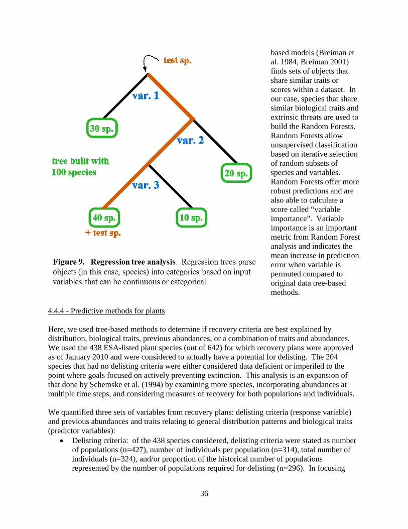
36
based models (Breiman et al. 1984, Breiman 2001) finds sets of objects that share similar traits or scores within a dataset. In our case, species that share similar biological traits and extrinsic threats are used to build the Random Forests. Random Forests allow unsupervised classification based on iterative selection of random subsets of species and variables. Random Forests offer more robust predictions and are also able to calculate a score called “variable importance”. Variable importance is an important metric from Random Forest analysis and indicates the mean increase in prediction error when variable is permuted compared to original data tree-based methods.
4.4.4 - Predictive methods for plants Here, we used tree-based methods to determine if recovery criteria are best explained by distribution, biological traits, previous abundances, or a combination of traits and abundances. We used the 438 ESA-listed plant species (out of 642) for which recovery plans were approved as of January 2010 and were considered to actually have a potential for delisting. The 204 species that had no delisting criteria were either considered data deficient or imperiled to the point where goals focused on actively preventing extinction. This analysis is an expansion of that done by Schemske et al. (1994) by examining more species, incorporating abundances at multiple time steps, and considering measures of recovery for both populations and individuals. We quantified three sets of variables from recovery plans: delisting criteria (response variable) and previous abundances and traits relating to general distribution patterns and biological traits (predictor variables):
• Delisting criteria: of the 438 species considered, delisting criteria were stated as number of populations (n=427), number of individuals per population (n=314), total number of individuals (n=324), and/or proportion of the historical number of populations represented by the number of populations required for delisting (n=296). In focusing

37
only on this restricted set of species, we recalculated metrics relative to delisting criteria that was also reported in the previous section (summarized in Fig. 7 above). Here, we recalculated these metrics just for the 438 species and present summaries in Table 6. As before, we present results with and without Hawaiian species (n=245) since those species represent a block that had nearly identical listing criteria (8 populations and 80, 100, or 300 individuals per population).
• Distribution data: Abundances were recorded (wherever available) at three points: historical, at time of listing, and at plan writing. Number of populations was recorded (wherever available) at two points: time of listing and at plan writing. Note that historical time period is vague but generally refers to a time prior to anthropogenic decline.
• Traits: eight distributional and biological traits were chosen either because they had been shown to relate to extinction risk and rarity but also were available for a sufficient number of species to allow analysis. These traits include Maximum plant height (m), maximum flower size (cm), plant life form, life history duration, reproductive mode, reproductive repetition, physiographic division, range area, listing status (Trait levels are shown in Table 7)
Note that the year the recovery plan was written was quantified, but exploratory analysis suggested it was not an important variable, so it wasn’t included in the formal analysis. Relationships between predictors and delisting criteria were analyzed using random forests as described above and calculating variable importance for each predictor variable. We also ran
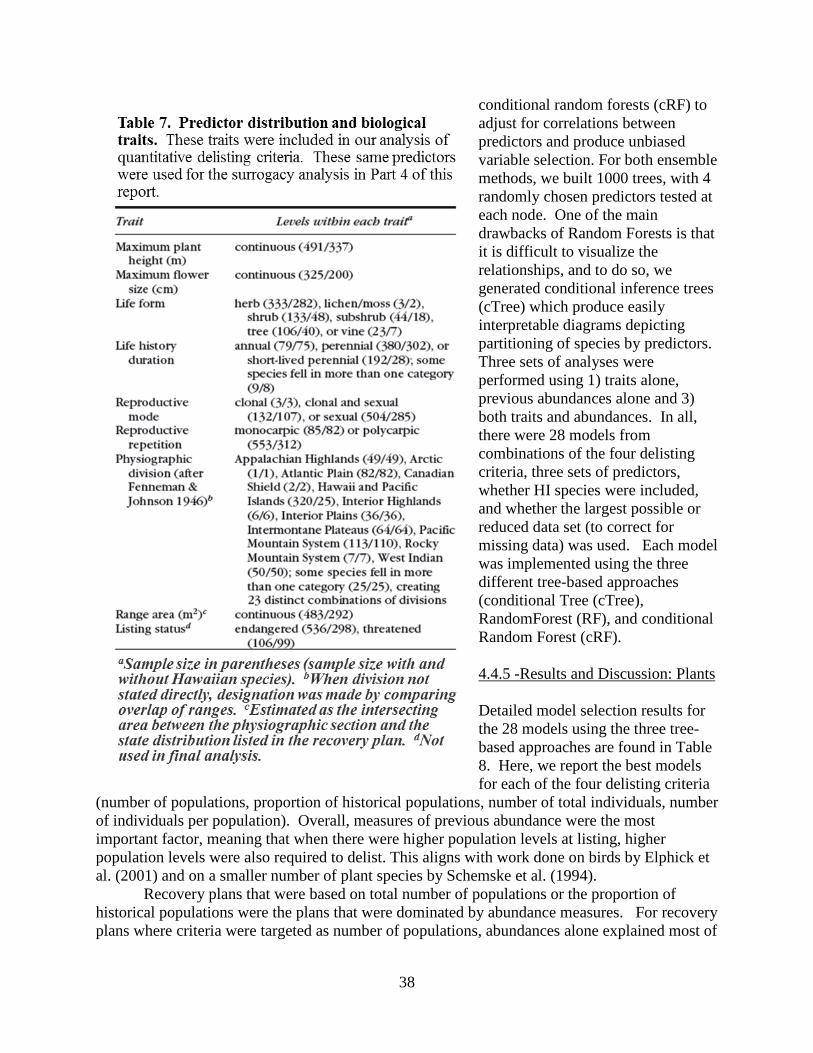
38
conditional random forests (cRF) to adjust for correlations between predictors and produce unbiased variable selection. For both ensemble methods, we built 1000 trees, with 4 randomly chosen predictors tested at each node. One of the main drawbacks of Random Forests is that it is difficult to visualize the relationships, and to do so, we generated conditional inference trees (cTree) which produce easily interpretable diagrams depicting partitioning of species by predictors. Three sets of analyses were performed using 1) traits alone, previous abundances alone and 3) both traits and abundances. In all, there were 28 models from combinations of the four delisting criteria, three sets of predictors, whether HI species were included, and whether the largest possible or reduced data set (to correct for missing data) was used. Each model was implemented using the three different tree-based approaches (conditional Tree (cTree), RandomForest (RF), and conditional Random Forest (cRF). 4.4.5 -Results and Discussion: Plants Detailed model selection results for the 28 models using the three tree-based approaches are found in Table 8. Here, we report the best models for each of the four delisting criteria
(number of populations, proportion of historical populations, number of total individuals, number of individuals per population). Overall, measures of previous abundance were the most important factor, meaning that when there were higher population levels at listing, higher population levels were also required to delist. This aligns with work done on birds by Elphick et al. (2001) and on a smaller number of plant species by Schemske et al. (1994). Recovery plans that were based on total number of populations or the proportion of historical populations were the plans that were dominated by abundance measures. For recovery plans where criteria were targeted as number of populations, abundances alone explained most of

39
the variation with 37-71% with the most important variable abundance at listing (Fig. 10). The model performed well with and without Hawaiian species. However, models including abundance and traits also were significant and explained 13-49% of the variability with

40
reproductive mode and repetition showing as the most important traits (Table 7). For Recovery Plans where criteria were targeted as proportion of historical populations, abundances alone provided the best model with 64-68% of the variation explained; however, in this case, historical population size was the most important variable (conditional tree not shown). For these delisting criteria, no other models were successful and only models with Hawaiian species were run.
However, we also found that traits were important alone or in combination with abundance for delisting criteria focused on numbers of individuals (or individuals per population). For recovery plans where criteria were targeted as total number of individuals, traits were more important than previous abundances alone (Table 7). In this case, the best models either included only traits, using either the full or reduced model (45-58% or 35-56% of variance explained respectively) or abundance and traits combined (31-56% of variance explained). For all these cases, significant models all included Hawaiian species (Table 7). For the model that included both abundance and traits, physiographic division was the most important predictor, with life form and duration also coming out as important traits along with the number of individuals at listing and recovery plan writing (Fig. 11). For recovery plans
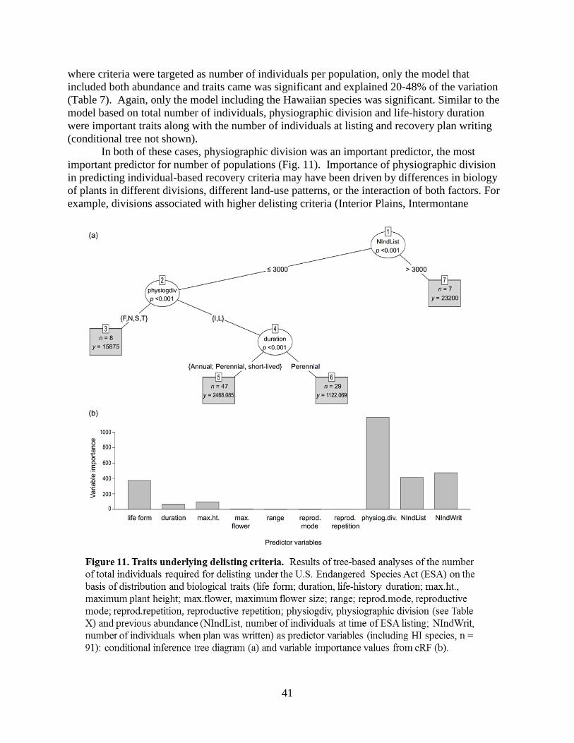
41
where criteria were targeted as number of individuals per population, only the model that included both abundance and traits came was significant and explained 20-48% of the variation (Table 7). Again, only the model including the Hawaiian species was significant. Similar to the model based on total number of individuals, physiographic division and life-history duration were important traits along with the number of individuals at listing and recovery plan writing (conditional tree not shown).
In both of these cases, physiographic division was an important predictor, the most important predictor for number of populations (Fig. 11). Importance of physiographic division in predicting individual-based recovery criteria may have been driven by differences in biology of plants in different divisions, different land-use patterns, or the interaction of both factors. For example, divisions associated with higher delisting criteria (Interior Plains, Intermontane

42
Plateaus, and Pacific Mountain System) tend to have a greater proportion of public land, which is subject to land uses that alter carrying capacity but is less threatened by uses that cause permanent conversion of habitat (e.g., residential, agriculture, or industrial development), than the eastern United States (Flather et al. 1998). Range and abundance of listed plant species in the interior and western divisions have declined less than those of species in other areas (see Fig. 5 in previous section on patterns of decline). A lower probability of land conversion and smaller population declines increase recovery potential in these divisions because a larger proportion of the historic habitat and range remains and can support more individuals (Kerr & Deguise 2004). The Hawaii and Pacific Islands division was associated with low species delisting criteria, potentially because this division is severely affected by habitat loss and degradation and supports species with naturally limited distributions and specific habitats. Thus, these patterns may reflect what is possible for conservation in each region rather than biological mechanisms. Differences between physiographic divisions may also have resulted from the particular species representing each division in our data set. The Atlantic Plain/Appalachian Highlands/Interior Plains division, which was consistently associated with low species delisting criteria, was represented only by the broadly distributed but locally rare species Isotria medeoloides. The recovery criterion for this species of permanently protecting 75% of known populations and increasing abundances in 25% of populations translates to delisting when 2420 total individuals are conserved (U.S. Fish and Wildlife Service 1992). 4.4.6 - Results and Discussion: Animals A similar analysis as above was carried out for animals, but data limitation was much more extensive than for plants. For example, out of 528 listed animal species with recovery plans, only 85 species had data on the prior abundances needed to predict number of populations required for delisting. Using a statistical imputing method, we assigned weighted median values to missing cells, in which the weights were based on values for other species placed in the same node. As with the listed plants above, we used predictors on past and present abundances (historical number of populations, number of populations at listing and when the recovery plan was written, and number of individuals at those time points), distributional data on habitat extent, and trait data including adult mortality, age at maturity, maximum lifespan, food habits, and mean body mass. Across all listed animal species with sufficient data for analysis (n=274), the conditional inference tree method explained 54.26% of the variance in number of populations required for delisting, and abundance variables (e.g., number of populations at writing and number of populations at listing) were important explanatory variables, although adult mortality was also a splitting variable. The conditional random forest methods explained only 40.14% of the variation and the number of populations at plan writing and historical number of populations were the most important predictors. Abundance and biological traits were poor predictors for the number of total individuals and the number of individuals per population that were required for delisting.
We also examined recovery criteria for three vertebrate groups separately: mammals (n=64), fish (n=112), and birds (n=102). Only the model for birds had high explanatory power, with other groups never yielding models that explained more than 10% of variance in recovery criteria. For birds, the conditional inference tree method explained 64.85% of the variance in number of populations required for delisting, and number of populations at writing and extent of habitat were the most important explanatory variable (Fig. 12a). However, conditional random
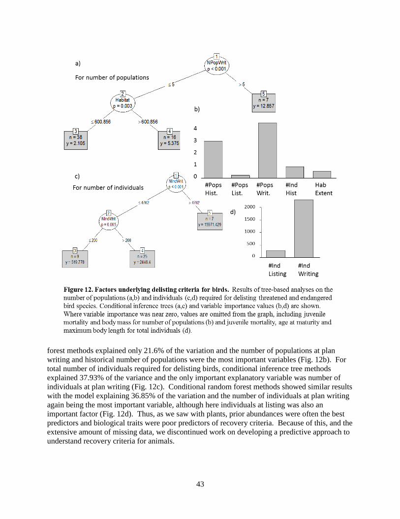
43
forest methods explained only 21.6% of the variation and the number of populations at plan writing and historical number of populations were the most important variables (Fig. 12b). For total number of individuals required for delisting birds, conditional inference tree methods explained 37.93% of the variance and the only important explanatory variable was number of individuals at plan writing (Fig. 12c). Conditional random forest methods showed similar results with the model explaining 36.85% of the variation and the number of individuals at plan writing again being the most important variable, although here individuals at listing was also an important factor (Fig. 12d). Thus, as we saw with plants, prior abundances were often the best predictors and biological traits were poor predictors of recovery criteria. Because of this, and the extensive amount of missing data, we discontinued work on developing a predictive approach to understand recovery criteria for animals.

44
4.4.7 - Summary
Although these methods were less successful for animals other than birds, the importance of previous abundances emerged as a major factor in both analyses, generally more important than traits. Dependence of recovery criteria on prior abundances has been considered problematic because such criteria are considered to not reflect species biology (Schemske et al. 1994; Elphick et al. 2001). We contend that relations between recovery criteria and previous abundance do not necessarily indicate recovery criteria are poorly formed and offer several explanations for the failure to find stronger relations between traits and recovery criteria. First, we may not have focused on the correct traits or not taken into account interactions between the traits. Weak associations may also emerge because extinction risk and recovery potential depend on combinations of traits and circumstance. Vagueness of the recovery criteria can also hamper our ability to rigorously quantify criteria, eroding our ability to find strong statistical links. Finally, recovery criteria are highly normative and influenced by societal value, political will, and competing economic pressures. Therefore, how recovery is defined is best seen as a combination of previous abundances, traits, threats, and political circumstances at the time that recovery criteria are set. 4.5 - Conclusions Taken in total, these papers show that existing recovery criteria are not predicted by the biological traits examined. Rather they are best predicted by prior abundances. As we have considered these findings with great thought, we have realized that expecting recovery criteria to be similar for biologically similar species may be fundamentally flawed. Despite its great intuitive appeal and underlying role in a number of areas in current ecology and evolution, there are many reasons why the expectation is unrealistic. The overriding realization emerging from our work is that is that scientists have not yet found a defensible approach by which extinction risk can be estimated as complex function of abundance, distribution, and extrinsic threat. Thus, there is no way to evaluate whether recovery criteria of 10,000 individuals in 10 populations for one species for which threats have been abated would yield the same probability of persistence for another species for which 50,000 individuals in 5 populations with some level of remaining threat.
Although the need to have more empirically based recovery criteria is recognized (Tear et al. 1993; Schemske et al. 1994), this context-dependent extinction risk and recovery potential continue to preclude establishing consistent recovery criteria, or even a way to determine whether criteria are consistent across species. Ideally, scientists and practitioners would determine an acceptable level of extinction risk for all species and then apply a science-based framework to translate that risk into quantitative recovery criteria for each species. Despite an excellent scientific foundation for understanding effects of life-history traits and external threats on relative extinction risk, methods for translating generalities to quantitative estimates are lacking. Population viability analysis (Shaffer 1981) offers the only quantitative method for risk assessment, but even proponents of these models do not consider them suitable for setting specific conservation criteria (Crone et al. 2011). A fundamentally new approach needs to be developed that weaves together a number of related fields, typically treated separately (e.g., determination of broad-scale correlates of rarity, past extinction patterns, or turnover at small

45
spatial scales; time series analyses; comparisons of traits in rare versus common or endangered versus secure species; and incorporation of stochastic processes), and thus integrates species biology, anthropogenic threats, and their interactive effects to comprehensively quantify extinction risk and develop criteria for its abatement. We present more progress on exploring the use of PVAs (Part 3), and then turn to the goal of developing methods for recovery planning when data are lacking (Parts 4-6).

46
5. PART 3: IMPROVING THE UTILITY OF POPULATION VIABILITY ANALYSIS IN RECOVERY PLANNING
5.1 - Background Population viability analysis is still considered by some scientists to be the “gold standard” in establishing defensible recovery goals. PVA is defined here as “an analysis that uses data in an analytical or simulation model to calculate the risk of extinction or a closely related measure of population viability” (Ralls et al. 2002). The appeal of PVA and related approaches lies in use of quantitative methods to forecast the future status of a population (Morris and Doak 2003) and to model both deterministic and stochastic elements of a system related to anthropogenic threats, management scenarios, and environmental conditions (Akcakaya and Sjӧgren-Gulve 2000). This framework also requires biologists to be more explicit in their reasoning, integrate knowledge from multiple sources, identify important model structures and parameters, and guide future data collection (Akcakaya and Sjӧgren-Gulve 2000). However, PVAs have also been criticized because uncertainty inherent in the modeling process may make it an inappropriate tool for assessing absolute outcomes or prescribing absolute population sizes (Crone et al. 2011; Reed et al. 2002). Uncertainty in PVA is particularly problematic when demographic data are limited (Beissinger 2002), which is typical for endangered species (Schemske et al. 1994). Table 9 shows characteristics that have been promoted as being critical components of an “ideal” PVA used for setting quantitative recovery criteria. Although Menges (2000) promoted use of PVA in plant conservation, his review of 95 plant PVAs revealed that most were not parameterized with data from enough individuals or years to capture variability and did not include important components such as stochasticity and metapopulation dynamics. Therefore, many did not meet the criteria of an “ideal” PVA laid out in Table 9. Further, depending on how data were collected, inference related to PVA output may only apply to the population from which the data came as well as the time-period in question. This is a particular problem when realistic estimates of error and variability are not available to be built into the model. In general, data availability is limited for reasonable estimates of the true variability that may exist across time and space, so researchers are often left to make assumptions about the error structure and build those into their models. So, while PVA remains a powerful tool for understanding underlying mechanisms and making predictions, it is also limited by data availability and ability to generalize across space and time are usually limited. These limitations have caused some to even question the validity of using PVA to inform conservation goals for TES (DeMaster et al. 2004). The PVAs described in Table 9 are based on classic PVAs that are built on demographic models, are mechanistic in nature, and demand a great deal of data on each life stage and transition. However, PVAs are a classically “data hungry” approach that demand data on multiple life stages and transitions that are difficult and costly to obtain, and model output can be sensitive to small changes in parameter estimates. Further, since parameters are generally estimated from intensive field studies, data usually come from a restricted spatial extent and usually only from a few years of data. However, time-series data on population size are much more common and often exist for several different populations. Further, new modeling techniques are improving our ability to estimate absolute or relative population sizes and correct for year to year differences in detectability (Mackenzie et al. 2002). Therefore, if output associated with PVAs could be estimated from time-series data, that would greatly expand our

47

48
ability to apply these approaches, and also potentially give a way to cross-validate data from more traditional mechanistic approaches.
Population viability analyses (PVAs) have now become a standard tool in conservation biology, with goals ranging from providing detailed guidance on management actions (Crouse et al. 1987) to simply characterizing the degree or nature of risk faced by populations (Morris et al. 2002; Fagan et al. 2001). Obtaining sufficiently detailed field data to parameterize models of population viability involves a challenging amount of work. Consequently, but unfortunately, for most species and situations, we lack the data required for all but the crudest PVAs. Indeed, it is telling that a synthesis found only 21 data sets (19 species) with sufficient data for full PVA assessments (Brook et al. 2000). These data sets, which contained substantial detail on population size- or age-structure, life history, and demography, are far more characteristic of focused efforts by academic researchers than of the cash-strapped monitoring efforts by governmental wildlife agencies and nongovernmental organizations upon which so much modern conservation action depends. Though helpful when available, such detailed demography and basic population biology data are often lacking for species of conservation concern. As a result, any full assessment of the utility of PVAs must examine their performance when faced with less detailed information.
When relevant data are available, one commonly used approach to developing a PVA is through the use of timeseries of censuses, population counts, or estimates of population size. Though still uncommon, long-term studies providing a continuous record of ‘count data’ occur more frequently than do in-depth demographic studies. Diffusion approximations (DAs) (e.g., Dennis et al. 1991, Holmes 2001) are one set of techniques that researchers have developed to estimate population vulnerability and extinction risk from limited data. The key to such approaches is the assumption of a simple stochastic exponential growth model and the estimation of the population growth rate and its variability from the year-to-year (or census-to-census) transitions in population size associated with such a model. These parameters, in combination with the most recent known population size, are then used to calculate the probability that a population will decline to extinction within a specified time frame. These models can also be used to discern additional information as well (Dennis et al. 1991), including profiles of quasi-extinction risk. Such profiles define the probability that a population will decline to each of a series of population sizes, of which extinction, or Nt=1, is but one of many potential values of interest (hence, “quasi-extinction”).
Diffusion-approximation models provide a tool for estimating quasi-extinction risk, although such models may be constructed and parameterized in a variety of ways ((Dennis et al. 1991); (Lande et al. 1998); (Engen and Saether 2000); (Holmes 2001)). One method of assessing the accuracy of DA models is to evaluate their performance in quantifying risk in real populations, as Ludwig (1999), Brook et al. (2000), and Ellner et al. (2002) have done. The general approach taken is a cross-validation analysis in which the first portion of a time series is used for estimating parameters, then the predictions of those parameterized models are evaluated by comparing them to the realized dynamics evident in the remaining portion of the time series. Brook et al. (2000) outlined the utility of applying cross-validation techniques to issues of extinction risk. They concluded that the good agreement between model predictions and realized dynamics evident in the evaluation portion of their time series was a strong endorsement of PVAs as a conservation tool. Ellner et al. (2002) criticized this conclusion, arguing that the results of Brook et al. (2000) fell far short of “predictive

49
accuracy” and instead merely demonstrated an absence of bias in ensemble—rather than species-level—estimates of probabilities of quasi-extinction. We have two goals for this section: 1) an exploration of the use of PVA in Recovery Plans and an analysis of the extent to which state-of-the-art methods are being employed and 2) the development of a new approach to PVA use in conservation planning that is based on time-series data and so doesn’t require detailed mechanistic data that are usually lacking. 5.2 - PVA in ESA recovery planning Our objective in this study was to reassess the actual and potential use of PVA in determining scientifically-based, measurable recovery criteria for endangered plant species listed under the ESA to determine if PVAs were being conducted or recommended as part of the recovery planning process. We also reviewed peer-reviewed studies containing plant PVAs (irrespective of focal species listing status) to assess whether the state of the art in PVA is sufficient to contribute to assessments of quantitative recovery criteria and if PVA design has improved since Menges’ 2000 publication. The work described in this sub-section is a summary of a manuscript by Zeigler and colleagues that is currently in press at Conservation Biology (See Appendix 2). 5.2.1 - Methods To assess use of PVA in endangered species recovery planning, we reviewed 258 final recovery plans for 642 plant species that were approved by USFWS prior to 30 June 2010. For each recovery plan, we searched for the keywords “population viability analysis”, “minimum viable population”, “matrix”, “model”, and “viability” and noted how PVA was discussed in applicable plans, including whether (1) the plan discussed a PVA study conducted previously or as part of the plan, (2) an existing PVA informed recovery criteria, (3) recovery criteria were written in the language of PVA (e.g., the population should have a specific probability of persistence for a set time period to be considered recovered), (4) PVA was recommended as part of the recovery strategy, or (5) PVA was recommended to determine, evaluate, or refine recovery criteria. Additionally, for the 251 listed plant species for which delisting was considered possible, we recorded qualitative statements in recovery criteria that were related to viability. Those results were presented earlier in Part 2 in the subsection on factors used to determine recovery goals. To assess if the state of the art in published PVAs and how they could be used as a strong tool for setting quantitative recovery criteria, we used ISI’s Web of Science database and the search engine Google Scholar to search for PVA-related peer-reviewed literature for plants (irrespective of the focal species’ listing status). We used the search terms “population viability analysis”, “viability,” and “matrix population model” to find studies published through December 2008. Publications that provided demographic information but no model of current or future population trends, extinction risk, or minimum viable population estimates (MVP) were excluded. We found 223 studies describing 280 PVAs for 246 plant species. To determine whether these models had attributes of an ‘ideal’ PVA (Table 9), we noted the type of model used, which could be an age- or stage- based matrix model, individual based model, or other model type (e.g., periodic projection matrix, equation-based model, reaction-diffusion model). We also noted if multiple models were explored to determine the sensitivity of PVA results to model structure. We determined if PVAs considered complex attributes of plant life history (e.g., seed bank, clonal reproduction, and plant dormancy) and if they incorporated

50
stochasticity, genetics, ecological processes/interactions (e.g., density dependence, natural disturbances), or external population drivers (e.g., threats or management actions). We also recorded the number of populations and years of observation used to parameterize PVAs. Finally, we noted whether perturbation analysis or model validation were used to explore the impact of parameter uncertainty on predictions. To determine if PVA design has changed since Menges (2000), we used chi-square tests to compare the number of PVAs published before (n = 116) and after (n = 164) 2001 that were parameterized with more than five years of data as well as the number of PVAs that incorporated stochasticity, disturbances/catastrophes, density dependence, metapopulation dynamics/dispersal, or genetics. In addition, for each focal species, we noted the listing status under the ESA (not listed, threatened, or endangered) and IUCN (not listed, critically endangered, endangered, vulnerable, lower risk, least concern, or conservation dependent), life form, and duration. We also recorded finite rate of population growth (λ), probability of and mean time to extinction for stochastic simulations, MVP size, and sustainable harvest levels as predicted by PVA models when given. When perturbation analyses were conducted, we noted the methodology used (sensitivity, elasticity, or life table response experiment) and the stage class (adult/reproductive/large plants, juvenile/non-reproductive/vegetative/medium plants, seedlings/saplings/small plants, seeds, or dormant plants) or life history process (stasis/survival, progression/growth, reproduction, germination/establishment/recruitment, retrogression, or clonal growth) deemed most important for population growth.
Finally, we evaluated within-species variability in PVA results based on methods, space, and time. For studies reporting population growth rates using different PVA methodologies or across different sites or years, we noted if rates were statistically different (as determined by the study’s author). We also calculated the arithmetic average, standard deviation, and percentage difference between minimum and maximum population growth rates to describe the magnitude of within-species variability for all studies, irrespective of whether authors statistically compared growth rates. 5.2.2 - Results and Discussion We found limited use of PVA in ESA recovery planning; only 15% of the 258 final recovery plans for 24% of the 642 listed plant species mentioned or recommended PVA. However, the concept of viability was nearly ubiquitous in recovery criteria; recovery plans for 233 of the 251 species for which delisting was considered possible included qualitative statements requiring viability in a broad sense (see Table 5 in Part 2). Nevertheless, most recovery plans simply recommended PVA for the recovery strategy, only 12 plans, representing 14 species actually included information on PVAs conducted either prior to or during plan writing (Fig. 13). Instead, most recovery plans simply recommended PVAs for the recovery strategy or for use in evaluating recovery goals (Fig. 13). However, despite the lack of PVAs specifically included or recommended in plans, nearly 97% of the 642 listed plant species suggest that more PVAs could be conducted in the future in that 97% of the 642 listed plant species have recovery plans that recommend monitoring or research related to demography, specific life history stages, and genetic viability as part of the recovery strategy (Fig. 14). Furthermore, demographic monitoring is specifically required in downlisting and delisting criteria for 98 and 97 species, respectively. This suggests a strong role for PVA or similar demographic models were assumed to be possible for recovery plan implementation (Fig. 14)

51
Most PVAs lacked many of the crucial elements of the best practices for implementing PVAs (Table 10) and, further, there has been little improvement since Menges’ 2000 review. In the 280 published plant PVAs, the typical model was an age- or stage-based matrix model (89% of PVAs) that focused on a species that was not listed under the ESA (92%). It was parameterized with <5 years of demographic data (69%) from a single population (53%) and did not include parameters for stochasticity (74%), genetics (95%), or density dependence (91%). The typical model did not include special components relevant to plant species such as seed banks (70%), vegetative reproduction (97%), or dormancy (95%) nor did it include threats (87%) or management strategies (90%). It did include perturbation analysis (59%) but did not evaluate multiple PVA methods (97%) or validate model results by comparing model predictions to actual population trends (95%). We also found that the number of PVAs published subsequent to Menges’ publication (2000) that considered density dependence, spatial factors, or genetics was not significantly different from the number prior to that publication (results not shown). However, significantly more PVAs considered stochasticity (32%; χ2= 8.0, p<0.05) and were parameterized with >5 years of data (34%; χ2= 4.3, p<0.05) following Menges’ publication. A synthesis of results from the PVAs presented some surprising patterns. First, the estimated population growth rates ranged substantially, ranged from 0.0004 for Dipsacus sylvestris (Werner and Caswell 1977) to 15.54 for Lobularia maritima (Pico et al. 2002), with a mean of 1.08 (sd 0.64; median 1.00). Further, whereas only 44% of PVAs reported growth rates less than one, 61% off the populations were actually declining based on other data. That seems

52
to suggest that the PVAs are either missing some crucial factor or the parameter estimates need to be refined. Surprisingly, only 11 of the plant PVAs reported MVP sizes which suggests that groups deploying PVA rarely use one of the features of this approach that allows defensible setting of recovery goals. Another useful feature of PVAs are you can vary parameter estimates once the model is built to determine which factors contribute most to variability in estimated growth rates. This feature allows the key traits to be identified and can act as a guideline as to which traits are most important in understanding population growth. Perturbation analysis conducted in 164 PVAs for 150 species indicated that population growth rates were most sensitive to changes in life history stages involving adults, reproductive individuals, or large plants (70% of species) followed closely by stages involving juveniles, non-reproductive/vegetative individuals, or medium-sized plants (67%). The most important demographic process for these species was stasis/survival (95%) followed by progression/growth (53%) and reproduction (32%). Percentages listed here do not sum to 100% because some studies indicated multiple stages or processes as being equally important for population stability and growth. In addition, these results may not be broadly reflective of important life history stages or demographic processes for all plants because the majority of plant species with PVAs included in our dataset were longer-lived perennials (86%), and adult survival is generally most important for longer-lived, late maturing species (Heppell et al. 2000). Studies that examined either within sites or across years showed substantial variability (Fig. 15) suggesting that PVAs constructed from few sites or during short time spans will not necessarily translate to novel sites or years. This suggests that even though PVAs are considered

53

54
the most rigorous approach to setting goals, results should be interpreted with caution, especially when applied to areas or time spans other than when data were collected. It is intuitive that PVA could inform recovery criteria by forecasting extinction or quasi-extinction probabilities over a specified time period, determining population status or trends, or establishing MVP sizes. However, these are precisely the applications considered to be the most inappropriate for PVA by prominent population biologists (e.g., Crone et al. 2011). Our results also show PVA’s lack of suitability for determining species-level recovery criteria due to data limitations and substantial shortcomings in PVA design that lead to unacceptable levels of bias and lack of precision as well as more fundamental characteristics of the PVA approach itself.
Data limitations include lack of demographic data from a sufficient number of individuals, populations, or years as well as lack of
information on life history traits that can influence model outcomes. We found that 81% of PVAs predicted growth rates for the same population that varied by more than 10% through time (Fig. 3). Typically, 15-20 years of data are needed to reliably estimate population growth trends or extinction risk (Che-Castaldo & Inouye 2011; Doak et al. 2005; Fagan et al. 1999), and reliably forecasting future extinction risk can require as much as a 5:1 ratio of observation to forecast years (Fieberg & Ellner 2000). Of the 231 PVAs we reviewed, only 4% were based on >15 years of data, and 69% were based on <5 years (Table 3). Although significantly more PVAs published after Menges (2000) were based on >5 years of data (Table 4), the median dataset length after 2001 was still only 4 years, indicating a need for continued improvement.

55
Limited spatial extent of datasets (i.e., the number of populations observed) is also problematic because population growth rates, viability, and underlying vital rates are highly context specific. Observations of multiple populations from throughout a species’ range over multiple years are needed to adequately capture species-level dynamics. However, 53% of PVAs in our review were parameterized based on observations of a single population. Because recovery plans typically specify that all populations conserved must be viable in a broad sense, evaluating probability of persistence in one or a few populations over short time frames contributes little to understanding whether this requirement is met and whether extinction is likely throughout all or a significant portion of the species’ range.
The need for 15-20 years of data from multiple populations to account for temporal and spatial variation in vital rates makes parameterizing even simple stage- or age-based models for all listed species a daunting task. Chronic lack of funding for endangered plants (Campbell 1991) has resulted in little existing demographic data (Schemske et al. 1994). Although USFWS recognizes the need for such data based on the fact that recovery plans for 97% of plant species recommend demographic monitoring and research, implementing these recommendations will require a commitment of funding and personnel that far exceeds historical levels (Male & Bean 2005).
Beyond lack of sufficient demographic datasets, lack of knowledge about key life history traits can also limit PVA applications. Models that exclude important population processes can overestimate population viability (Lindenmayer et al. 2000; Melbourne and Hastings 2008) and yield inaccurate projections of population dynamics (Courchamp et al. 1999; Grimm et al. 2005; Letcher et al. 1998). Features that are known to be important drivers of population dynamics for plants (Boyce 1992; Doak et al. 2002; Reed et al. 2002) are often difficult to quantify (Crone et al. 2011); in our study, most models did not consider stochasticity (74% of PVAs), genetics (95%), density dependence (91%), seed banks (70%), vegetative reproduction (97%), or dormancy (95%). As with lack of demographic data mentioned above, a greater commitment to research on endangered plant species could reduce the severity of this issue.
Even if data availability and model complexity were improved, many population biologists consider PVA approaches inappropriate for setting absolute conservation targets (Beissinger and Westphal 1998; Crone et al. 2011). One of the most fundamental mismatches between the paradigm of PVA and recovery planning is that models tend to focus on impacts of intrinsic demographic processes (e.g., pollen limitation, inter-annual variation in seed germination, or seedling survivorship) whereas extinction risk is often more affected by extrinsic large-scale and chronic human-mediated threats, such as resource extraction, exotic species introductions, and land-use change (Lawler et al. 2002). In addition, threatening processes can cause declines in population abundance, numbers of whole populations, and extent (i.e., area of habitat or range, with or without loss of whole populations).
Alternative modeling techniques that may be more robust to limited datasets have also been suggested. Integral projection models produce less biased and more precise population growth rate estimates than matrix models for small datasets (e.g., ≤300 individuals; Ramula et al. 2009), but they still do not overcome issues related to short time series. PVAs based on species occurrence rather than abundance offer a potential solution because presence and count data are more widely available than stage- or age-based data (Skarpaas & Stabbetorp 2011). In the next section, we explore the potential for specific recovery targets to be extracted from a PVA model that is designed for corrupted data sets, often the data that are available for recovery planning.

56
5.3 - PVA analysis using time-series data to estimate conservation targets While PVA remains an important tool for supporting conservation goals, the above work shows the limitations in applying that technique, often due to data limitations for an extremely data-hungry process. Here, we build upon the idea that time-series data on population trajectories produces visible trends generated from the mechanistic processes that underlie the standard PVA, so that it should be possible to make predictions about future trajectories based on observed patterns. While this approach has been used to implement PVAs whose sole goal is to predict population trajectories (Humbert 2009), these do not produce the specific parameters necessary to be able to estimate conservation targets like a Minimum Viable Population size or the probability of reaching an extinction or quasi-extinction threshold.
Here, we present work detailing an approach to allow us to extract parameters relevant to the establishment of recovery criteria, traditionally only available through data-hungry mechanistic PVAs, via use of time-series data only without the need of data on any specific biological mechanism. The approach is based on the idea that certain average properties of stochastic processes may be predictable even when the details of the underlying process are unpredictable and/or unknown. The key is to find statistical properties that are convergent over a broad class of plausible population dynamics. Convergent statistical properties are at the foundation of classical statistical inference. Our goal was to extend this type of reasoning to the estimation of a specific property of stochastic population trajectories: the probability of decline below a pre-defined threshold. As this metric does not measure absolute extinction per se, we use the term quasi-extinction (Ginzburg et al. 1982). Quasi-extinction probabilities are a widely used risk metric by conservation and management organizations. For example, the World Conservation Union’s IUCN risk criteria (Mace and Lande 1991) and the proposed quantitative criteria for the U.S. Endangered Species Act (DeMaster et al. 2004) rely on quasi-extinction probabilities. For this paper, we consider only quasi-extinction thresholds above the level at which demographic stochasticity and Allee effects become important. These factors accelerate the decline toward absolute extinction, which differs in many fundamental ways from the decline to a critical threshold (Gilpin and Soule 1986; Lande et al. 2003; Fagan and Holmes 2006).
Here we build on past work showing that exponential growth models can be estimated from corrupted data sets (Holmes 2001, Holmes and Fagan 2002) and used to separate dynamic population variance from observation error using a model called the Corrupted Stochastic Growth model (hereafter, CSEG). The CSEG model is written as the coupled system of equations
where Xt is the true (unobserved) population size, Nt is the observed population size, and µ is the mean population growth rate. Stochastic process error, σp, which represents underlying year-to-year environmental variation, is modeled as a Normal distribution with standard deviation σp. Stochastic non-process error (e.g., observation error), is denoted σnp, and is modeled as a Normal
( )
( )npnp
tnp,tt
pp
tp,tt
β,σ~NεwhereεXN
,σ~NεwhereεμXX
111
1
loglog
0
loglog
+++
+
+=
++=
( )
( )npnp
tnp,tt
pp
tp,tt
β,σ~NεwhereεXN
,σ~NεwhereεμXX
111
1
loglog
0
loglog
+++
+
+=
++=
Eq. 1

57
distribution with mean β (the mean observer bias) and standard deviation σnp. We extended this method to be able to estimate quasi-extinction profiles. 5.3.1 - Methods To develop a model able to extract parameters that are relevant to setting management objectives, we synthesized two bodies of theoretical research: the stochastic convergence properties of population processes and the estimation of stochastic models. We began by identifying a simple stochastic model (a stochastic exponential model overlaid with Gaussian errors) that approximates the relationship between quasi-extinction risk, threshold (meaning a critical population level at which extinction risk increases sharply) and forecast length. Our model of quasi-extinction includes observed population trajectories and models future population counts of forecast length, T. Thus, we are able to forecast the probability of “future” quasi-extinction given the observed counts by summing over the set of all possible past trajectories. The expected quasi-extinction rate is thus the expected probability of quasi-extinction observed by selecting a past trajectory randomly from the past trajectories that particular process could produce. It measures the propensity of a population process to produce quasi-extinctions.
In developing this new method, our main goals are to be able to extract four critical parameters: population trend, error estimates parsed into observational and process error, and an estimate of a minimum population needed to keep from falling below a quasi-extinction threshold. We begin by developing the model for the simplest population structure, one that is regulated by density-independent processes and includes no age- or stage- specific structures. We then adapt that model to be able to be used with real time-series data accounting for the types of noise typically found in these datasets. This step will allow us to apply the model to real data sets that are likely to be available to managers in real-world conservation situations that tend to contain errors and flaws. We then will adapt this more realistic model to complex population structures such as ones that include age- or stage-structured data or are assumed to have density-dependent processes. After developing these models, we apply them to real data and explore the best approaches to their applications using real-world data with common problems found, especially for species of conservation concern. We omit detailed methods and results for this report and focus instead on the results most pertinent to this project, but those details are available in Holmes et al. (2007).
5.3.2 - Results and Discussion We were able to use the CSEG model to output quasi-extinction probabilities for a broad class of processes that are known to underlie many observed population counts. This included examples on a stage-structured species (Chinook salmon), using a stochastic Ricker model, and also a community model with four interacting species. Under all these circumstances, the CSEG model was able to produce probabilities of reaching a quasi-extinction level that was either based on a specific population size (Fig. 16a) or a proportion of the original population size (Fig. 16b). These outputs could be used to set conservation targets such as a Minimum Viable Population size. It could also be used to determine a population’s current trajectory and how much of the observed variability is due to observation vs. process error.

58
In addition to developing a theoretical CSEG approximation for multiple stochastic processes, and showing it was possible to produce the four key parameters, we also used the data to test CSEG forecasts on real time series data for our key test datasets, all of which represent populations of conservation concern. To do this, we developed cross-validation simulations of the expected quasi-extinction probability as a function of forecast length to see how closely actual decline probability from the simulations matched estimates from the CSEG models for the Chinook salmon, Ricker, and community datasets (Fig. 17). We found that the CSEG model was able to capture these probabilities well, although the model did better for salmon (Fig. 17a-c) overall and when longer time periods were used overall (Fig 17). However, the modeling approach did not work well in all situations; for instance CSEG did not perform well when populations fluctuated slowly around a mean.
Overall, we found this method to be a promising approach to developing conservation targets when detailed mechanistic data necessary for standard PVAs are lacking. We have shown that simple stochastic approximations can model a particular ensemble property, the risk of quasi-extinction. We have focused on the CSEG model and shown how the CSEG can accurately approximate quasi-extinction risks across different forecast lengths and risk thresholds, for a variety of population processes. Using simulations and 20 years of data, we illustrated that CSEG estimates of quasi-extinction risk can have relatively low bias and 95% CIs that are much smaller than (0,1) – particularly for declining and rapidly fluctuating populations. We crossvalidated these results using a large dataset of abundance time series from species of conservation concern. Although we did find this approach to be powerful for many situations, we did highlight some areas where model improvement in necessary. However, we were able to find an approach that was generally free from biased results even when biological mechanisms were completely

59
ignored, often a criticism of simple PVA models. Another criticism that has been leveled against PVAs is that the data used are often riddled with errors. While this is true, here we present a method that works well with data sets that include errors that are common in field studies and we showed that it performed well in at least some circumstances. While there are many challenges still to overcome in building tractable approaches to forecasting population trajectories, we present a new approach that we hope can add a powerful tool for managers struggling to develop defensible conservation targets when only time-series of population sizes are available to them. 5.4 - Conclusions Currently, the only relatively standardized method to determine species-specific quantitative recovery criteria is the population viability framework based on minimum numbers of

60
individuals required for a specified probability of persistence (Favreau et al. 2006). Vital rates estimated from demographic approaches can be used to determine whether populations are on trajectories toward persistence versus extinction (Schemske et al. 1994) and structured population models can identify stages in the life cycle that are most important to population growth and the degree to which they are affected by stochasticity (Melbourne and Hastings 2008). However, from a practical standpoint, use of population viability analyses (PVAs) for establishing recovery criteria and management actions is precluded for most species due to intensive information requirements. In fact, PVAs have only been used to help determine downlisting and delisting criteria for five listed plant species (in two recovery plans), and included in the description of basic natural history for only nine listed species. Yet many consider the use of PVA to be inappropriate for setting absolute minimum numbers and suggest that it should only be used for comparative risk analysis (Beissinger and Westphal 1998; Flather et al. 2011; Reed and Shine 2002; Crone et al. 2011). In this section, we were able to highlight some drawbacks and strengths of PVA, as it is currently practiced on plants and also present a new approach that may allow PVA approaches when demographic data are lacking.

61
6. PART 4: INFERRING RECOVERY CRITERIA FOR POORLY-STUDIED SPECIES
6.1 - Background Conservation work to date has jumped between generic conservation rules and expensive, time-consuming, and often unattainable single-species PVAs, without regard for any intermediate analytical framework. For instance, without specific demographic information, conservation decision makers often apply various kinds of general rules of thumb to generate recovery goals. Even today, workers quote the well-known 50/500 and 500/5000 rules for effective population size targets. Such general rules can provide useful guidelines, but their invariant application across taxa with widely varying life histories and ecological characteristics is problematic. Although it may be intuitively obvious that the number of individuals needed to conserve an endangered insect is vastly greater than to conserve a bear population, the reality is that we still lack guidance on coming up with more species-specific criteria. Our goal was to develop a framework to account for the fact that for each species, extinction risk and recovery potential result from a combination of intrinsic factors (e.g., demography, life history, genetic diversity, ecological requirements, and range size) and extrinsic factors (e.g., types of threats; extent, magnitude, and duration of reductions in range and population size). To date, the balance of these individual factors, as it varies across species is poorly understood (e.g., Murray et al. 2002a). In originally undertaking this project, our goal was to provide a framework for quantifiable recovery goals and practical approaches to recovery planning by using this idea. In our initial framework, we planned to use a database amassing information from TES and well-studied species to leverage information across species and develop an analytical model that would produce a defensible estimation of the best recovery goals when on-the-ground or species specific data are lacking to parameterize data-hungry models (Fig. 18). Unfortunately, our experience was that there still are not enough species-specific data to allow this cross-species modeling approach. The lack of data was exacerbated by the fact that species do appear from our analyses to be fairly unique. This lack of congruence between traits, population trends, threats, and recovery criteria demanded even a higher degree of data on each species if this approach was to be successful. This made the lack of data availability even more problematic. Below, we show the results of multiple attempts to link traits, abundances, and threats and show that we were never able to design an approach that was able to compensate for the lack of data. While most of the work in this section shows a frustrating lack of successful results, they highlight an important challenge to conservation biologists and also highlight the need to continue filling in knowledge gaps across species, population dynamics, and threats throughout regions and landscapes. In the final section of this report, we describe an approach that harnesses evolutionary pathways to understand the distribution of traits across related species and can be used to help fill in gaps in knowledge in a robust way. For our attempts at harnessing current data, we used tree-based methods which are described in more detail in section 2 (see page 34), but specific details are given for each section. Then, we show the main results from our attempts to build comparison sets for our Proof of Concept bird and plant taxa. Finally, we show that even the more modest goal of trying to identify surrogates between well and poorly studied taxa met with the same result, species were too unique and we did not have enough data on traits.

62
6.2 - Comparison sets to infer recovery criteria for species with similar traits and threats Our approach to develop comparison sets had three major steps: 1) Use tree-based approaches to develop comparison sets for all TES species, 2) Determine if the comparison sets were statistically significant and stable, and 3) Identify if the species that were members of a stable and significant comparison set shared similar recovery criteria or similar quasi-extinction thresholds. We developed and tested this method on two taxa for which we had the most data: plants and birds. Throughout this section, we will present results separately for these two groups.

63
Step 1: Using tree-based approaches to develop comparison sets Comparison sets of species were developed using unsupervised random forest methods (see page 32) to distill data on life history traits, geography, and threats into a matrix of pairwise distances among species, the ‘proximity matrix’. To do this, we used the output of the random forests analysis to develop a “proximity” matrix showing how similar a focal species (e.g., a listed species) was to other listed or well-studied species in multivariate trait / threat space. Proximity in this context is quantified as the proportion of 1000 trees in the random forest runs in which two species fall into the same leaf as the underlying trait/threat matrix is sampled and permuted. Thus, the comparison sets are groups of species that share a suite similar biological traits and extrinsic threats. We then developed a proximity graph for each species from the proximity matrix. This graph allowed, for each focal species, an assessment and visualization of the ranked similarity of all other species by their proximity score relative to the focal species (Fig. 19). Step 2: Determine if sets are significant and stable
We assessed the statistical significance of each species’ membership in a comparison set via randomization tests that determined whether the proximity score between a focal species and a potential comparison species was robust to random sub-setting of the underlying trait/ threat matrix. Our goal here was to identify those species whose proximity to a focal species did not hinge on one or a few traits or threats that might be absent from a given trait/threat matrix given typical levels of incompleteness of the conservation databases. Significant comparison species were those whose proximity scores relative to the focal species were in the top 5% of such proximity scores that could be calculated, given the data available in the trait-threat matrix for those randomly constructed sets of the same size. To emphasize this point, a significant proximity score was not judged by its raw magnitude, but rather its magnitude relative to the other proximity scores that could be calculated given an assumption about how extensive the underlying trait/threat data matrix was. As a result, in a rank proximity graph (Fig. 20) significant comparison species (those species denoted by vertical lines in the figure) could be separated by runs of non-significant comparison species whose proximity to the focal species was sensitive to the scope and content of the available data matrix (Fig. 20a).

64
Statistically proximate species could be part of a comparison set for the focal species because their similarity relative to the focal species is robust to randomization of the multivariate trait/threat matrix. However, to be truly useful in any predictive context, we would also need a set of comparison species (i.e., a comparison set) to be stable with regard to the randomization. That is, we need the species in a comparison set to stay together as a group with regard to their proximity relative to the focal species as the trait/threat matrices are manipulated. Thus, not all species that are statistically proximate to a focal species could feasibly belong to a comparison set because the component species could differ wildly relative to one another (as a function of how much data was available) with regard to the proximity magnitude observed. We considered sets of >5 species with contiguous proximity values to comprise a stable comparison set for a focal species (Fig. 20b). Delineated in this way, stability of comparison sets is a stringent criterion, but it yields comparison sets that are relatively robust both to the content of the trait/threat data matrix and to inclusion or exclusion of species in the database as judged by ‘leave-one-species-out’ jackknifing.
To assess how well these comparison-sets associate with quantitative recovery criteria, we used two sets of data we have gathered. First we used time series obtained for over three hundred populations of birds (77 distinct species). We used the CSEG model (Part 3) to compute minimum viable population sizes (MVPs) from the time series data. Second, for 642 listed plant species with recovery plans, we looked at changes in the number of populations and the total number of individuals with the goal of expressing recovery criteria in these two quantities jointly.
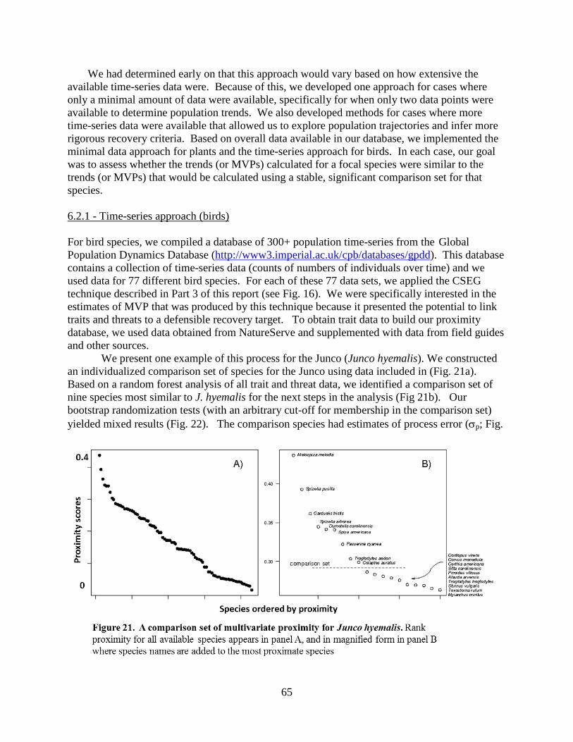
65
We had determined early on that this approach would vary based on how extensive the available time-series data were. Because of this, we developed one approach for cases where only a minimal amount of data were available, specifically for when only two data points were available to determine population trends. We also developed methods for cases where more time-series data were available that allowed us to explore population trajectories and infer more rigorous recovery criteria. Based on overall data available in our database, we implemented the minimal data approach for plants and the time-series approach for birds. In each case, our goal was to assess whether the trends (or MVPs) calculated for a focal species were similar to the trends (or MVPs) that would be calculated using a stable, significant comparison set for that species. 6.2.1 - Time-series approach (birds) For bird species, we compiled a database of 300+ population time-series from the Global Population Dynamics Database (http://www3.imperial.ac.uk/cpb/databases/gpdd). This database contains a collection of time-series data (counts of numbers of individuals over time) and we used data for 77 different bird species. For each of these 77 data sets, we applied the CSEG technique described in Part 3 of this report (see Fig. 16). We were specifically interested in the estimates of MVP that was produced by this technique because it presented the potential to link traits and threats to a defensible recovery target. To obtain trait data to build our proximity database, we used data obtained from NatureServe and supplemented with data from field guides and other sources.
We present one example of this process for the Junco (Junco hyemalis). We constructed an individualized comparison set of species for the Junco using data included in (Fig. 21a). Based on a random forest analysis of all trait and threat data, we identified a comparison set of nine species most similar to J. hyemalis for the next steps in the analysis (Fig 21b). Our bootstrap randomization tests (with an arbitrary cut-off for membership in the comparison set) yielded mixed results (Fig. 22). The comparison species had estimates of process error (σp; Fig.
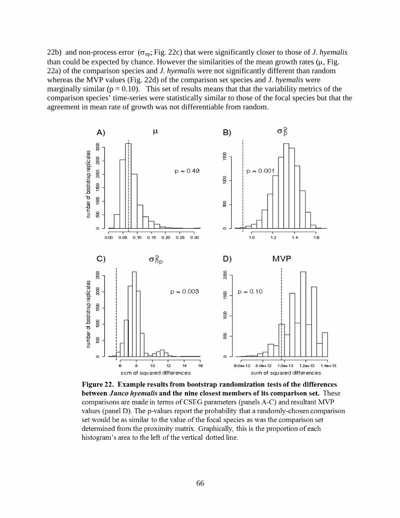
66
22b) and non-process error (σnp; Fig. 22c) that were significantly closer to those of J. hyemalis than could be expected by chance. However the similarities of the mean growth rates (µ, Fig. 22a) of the comparison species and J. hyemalis were not significantly different than random whereas the MVP values (Fig. 22d) of the comparison set species and J. hyemalis were marginally similar (p = 0.10). This set of results means that that the variability metrics of the comparison species’ time-series were statistically similar to those of the focal species but that the agreement in mean rate of growth was not differentiable from random.

67
We repeated the process outlined above and developed comparison sets for each of the 77 bird species. We then used our randomization technique to determine if we could find stable and significant sets for each of the species. Unfortunately, when looking at all 77 species, only about 20 had statistically significant comparison sets, and of those, fewer than 10 were both significant and stable (Fig. 23). The pattern we found for the Junco, namely success in cross-characterizing measures of variability using stable significant comparison sets but inability to estimate the means, occurred regularly in application of this approach to other bird species. The low number of species for which we could find comparison sets precluded us from proceeding to the next step in our process, inverse problem modeling (Fig. 18).
6.2.2 - Minimal data (plant) approach For 642 listed plant species with recovery plans, we looked at population changes based on two metrics: 1) the number of populations and 2) the total number of individuals. Our goal was to express recovery criteria in these two quantities jointly. For many plant species we were able to extract information from federal listing documents and recovery plans on number of populations and individuals at 1) the time of listing and 2) the time at which the recovery plan was written (for example, see Figs. 6 and 7). We then tested whether the nature of species’ declines in terms of populations and/or the number of individuals was a function of the types of threats a species
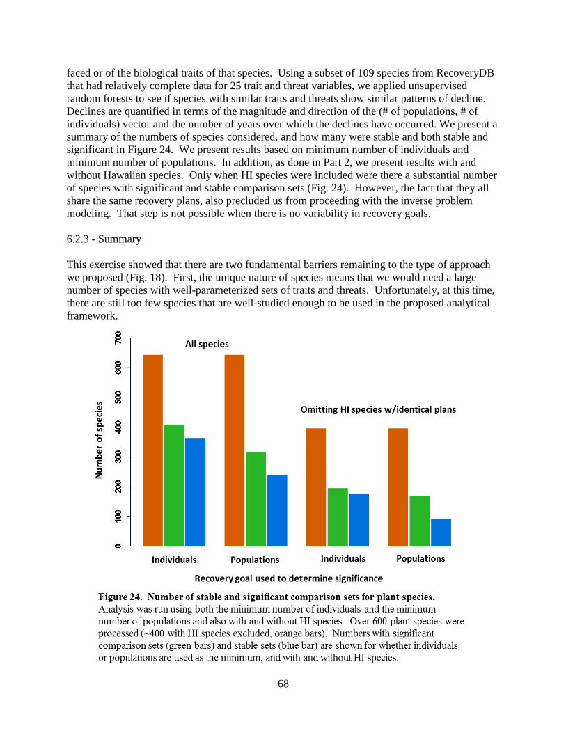
68
faced or of the biological traits of that species. Using a subset of 109 species from RecoveryDB that had relatively complete data for 25 trait and threat variables, we applied unsupervised random forests to see if species with similar traits and threats show similar patterns of decline. Declines are quantified in terms of the magnitude and direction of the (# of populations, # of individuals) vector and the number of years over which the declines have occurred. We present a summary of the numbers of species considered, and how many were stable and both stable and significant in Figure 24. We present results based on minimum number of individuals and minimum number of populations. In addition, as done in Part 2, we present results with and without Hawaiian species. Only when HI species were included were there a substantial number of species with significant and stable comparison sets (Fig. 24). However, the fact that they all share the same recovery plans, also precluded us from proceeding with the inverse problem modeling. That step is not possible when there is no variability in recovery goals. 6.2.3 - Summary This exercise showed that there are two fundamental barriers remaining to the type of approach we proposed (Fig. 18). First, the unique nature of species means that we would need a large number of species with well-parameterized sets of traits and threats. Unfortunately, at this time, there are still too few species that are well-studied enough to be used in the proposed analytical framework.

69
6.3 - Testing surrogacy assumptions: Can TES be grouped by traits and abundances? We found two main barriers to developing robust comparison sets to formally model the most defensible recovery criteria for species that have not been well studied is a lack of trait data to link the comparison sets together, but also that species are fairly unique in terms of their characteristics. This brings the question of whether or under what circumstances species can act as surrogates for each other for any use. Although the process we went through in this project is similar to the one above, our goals were slightly different. Above, we were looking for any species that could reasonably be linked together with a set of species that shared similar traits, threats, and recovery criteria to actually develop a model that would output a predicted “best” recovery target. Here, we tried to determine the extent to which one well-studied species could be used as a surrogate for another group of threatened and endangered species based on shared traits and abundance trends. If so, this one species could be the focus of conservation efforts and other species could be assumed to be protected or that the same recovery targets would be appropriate. In the broadest sense, surrogate approaches encompass all methods that apply principles from theory in ecology, population biology, and population genetics to determine conservation strategies in absence of species-specific information (Caro and O'Doherty 1999; Noss et al. 1997; Niemi and McDonald 2004). Surrogate species may be chosen based on a range of biological similarities with target species. They may overlap with target species in terms of ecological requirements or geographical ranges (indicator and focal species: Caro and O'Doherty 1999; Lambeck 1997), control target species abundance through trophic interactions (keystone species: Mills et al. 1993; Sergio et al. 2008), have close phylogenetic relationships with targets (species groups: Wiens et al. 2008) or have broad ecological requirements that encompass those of many species (umbrella species: Caro and O'Doherty 1999;Wilcox 1984; Fleishman et al. 2001). Based on these biological relationships and similarities, benefits from protection or management of surrogates are inferred to extend to target species. Thus, use of surrogate species for conservation planning employs the assumption that species sharing biological traits or relationships will also be similar in terms of their distribution, abundance, or response to management. Critics have long contended that surrogate approaches are ineffective because these underlying assumptions are likely unmet in most applications (Caro et al. 2005; Landres et al. 1988; Lindenmayer and Likens 2011; Murphy et al. 2011; Simberloff 1998). Further, in many cases the assumptions are not explicitly stated, and when they are stated they are rarely tested. As a result, the potential utility of surrogate approaches for most species is unknown. The few studies testing surrogacy assumptions for reserve selection have found no or weak correspondence between the presence, abundance, or richness of surrogates and those of the target taxa (Andelman and Fagan 2000; Lewandowski et al. 2010; Rodrigues and Brooks 2007). Selection of conservation sites based on one taxonomic group rarely represents other groups well and the degree of spatial overlap between groups is idiosyncratic (Chase et al. 2000; Brooks et al. 2001; Gladstone 2002; Saetersdal and Birks 1993; Scott et al. 2010; Virolainen et al. 2000; Williams et al. 2000). Thus it is essential to continue testing assumptions to determine if there are circumstances in which the use of surrogates is appropriate (Lindenmayer and Likens 2011). In the case where a common or well-studied species is chosen to represent the demographic trends or management responses of a group of listed species, two specific assumptions must be met.

70
First and fundamentally, there must be groups of threatened and endangered species that are sufficiently similar in multiple characteristics and/or threats to form identifiable groups that would justify representation by a surrogate species. Second, the groups of species must respond similarly to management and threat abatement as the surrogate species. In this study, we tested the first assumption by searching for groups of species with similar characteristics in the threatened and endangered plant species listed under the ESA. In addition to allowing potential representation by surrogates, groups of biologically similar listed species may share similar conservation needs and thus may be managed as a group to facilitate recovery planning. In this study, we used tree-based statistical models to examine whether listed plant species can be grouped based on a set of biological traits alone, their previous abundances and patterns of declines alone, or a combination of traits and abundances. This analysis will determine whether there are identifiable groups of listed species, and if so, identify traits that are important for defining these groups. 6.3.1 - Methods We compiled data on previous abundances and biological traits from recovery plans for the 642 listed plant species with final approved plans as of 31 December 2009. We recorded the number of historically known populations, number of populations at listing, number of populations at plan writing, total number of individuals at listing, and total number of individuals at plan writing. To quantify the pattern of decline for each species, we calculated the proportion of historical populations remaining at plan writing and that at listing, the proportion of populations at time of listing remaining at plan writing, and the proportion of individuals at time of listing remaining at plan writing. A summary of those metrics are shown in Table 11. We collected data on the same eight biological and distributional traits (also referred to here as “traits”): maximum plant height, maximum flower size, life form, life history duration,

71
reproductive mode, reproductive repetition, physiographic division, and range area. Specific levels for each trait category are shown in Table 7.
6.3.2 - Analysis
To examine whether listed plant species can be grouped based on similarities in traits, prior abundances representing patterns of declines, or a combination of traits and abundances, we used the random forests, which is a tree-based method of analysis (see page 34 for a general background). In this case we used an uninformed RF the data are modeled without a response variable to assess whether there is inherent structure in the data. The original dataset is classified as group one and a second group of data is created through random permutation of the original data, and RF is used to re-assign the combined data into two groups based on predictor variables. If there is structure in the original data, RF will correctly reassign the same groups with error rate <50%. By convention, <40% error indicates significant grouping whereas higher error rates indicate random group assignment. We used the randomForest function in the R package randomForest (Liaw and Wiener December 2002) to run RF. For each analysis we built 1000 trees with four randomly chosen predictor variables tried at each node (mtry=4), except in the individual-based abundances model in which there were only three total predictors (mtry=3). Different mtry values were tested and produced similar results (not shown). To assess model accuracy, we used the out-of-bag classification error (OOB error), which was the mean squared error calculated using only the observations that were not used to build the individual trees. We performed three sets of analyses: classification of species based on traits alone, previous abundances alone, and both traits and abundance. For models including abundances as predictors, we also ran separate models including only population-based abundances or only individual-based abundances to examine whether the measure of abundance affected classification. Because all examined variables were missing data from at least one species, each analysis used a different subset of the data ranging from 70 to 352 species (Table 12). 6.3.3 - Results
We found no evidence of grouping among listed plant species based on biological traits, abundance or traits and abundance (Table 12). Variable importance values for all traits were negative for biological traits (Fig. 25a) and mostly negative for abundance traits except for some marginally positive values (Fig. 25b). Results were similar when the analysis included only population-based abundances (Table 12). There was, however, significant grouping in the analysis including only individual-based abundances (OOB error = 29.4%; Table 2), and the number of individuals at plan writing had the highest variable importance value (mean decrease in model accuracy from variable permutation are -0.12, 0.06, and -0.06 for the number of individuals at time of listing, number of individuals at time of plan writing, and number of individuals at time of plan writing remaining at time of listing, respectively). 6.3.4 - Discussion Our results are similar to the ones we found above and are therefore not surprising. Our results demonstrated that ESA-listed threatened and endangered plant species cannot be grouped based

72

73
on their biological traits or most of the abundance variables we examined. Further, the lack of similarity among listed species may indicate a true difference in terms of their intrinsic characteristics and patterns of decline, but it may also be due to data limitations even though we went to great lengths to develop a comprehensive database and statistically account for residual gaps in data available across species. For example, each of the traits examined had missing data for many of the species, and actual similarities may not have been illuminated due to insufficient data. However, managers tasked with choosing surrogate species will be faced with the same level of data deficiency given that our data come from actual recovery plans. The overall lack of grouping suggests low potential for widespread use of surrogacy to guide recovery planning because species do not meet the fundamental requirement of forming biologically similar groups. However, the lack of grouping may also have resulted because listed species represent a subset of plant species that share similar values for the traits examined and cannot be further subdivided. This was likely true for using abundance as an indicator. For example, they all have relatively low abundances and have experienced declines, which are related to their threatened and endangered status. If their threatened status results in a small range of values for each trait represented in our dataset, there may not be sufficient variation among species to split them into more refined groups. It is possible that comparing non-listed and listed species would have presented a broader range of traits and enabled grouping species by traits. However, such groupings would not meet our goal of finding suites of listed species that can be managed similarly or that could have similar recovery criteria. However, lack of trait diversity doesn’t seem to be a likely cause because many traits were represented in the database

74
6.4 - Conclusions Our attempt to build comparison sets showed that we are not yet at the point where we have enough data to employ a data-intensive approach to predicting recovery criteria. We were never able to produce enough stable and significant comparison sets to proceed with the inverse modeling portion of our analytical flow (Fig. 18). Considering our focus was on relatively well-studied taxa (plants and birds), this does not bode well for applying the method broadly at this point. Yet even exploring simpler surrogacy approaches proved elusive. Previous studies testing the assumptions of surrogate approaches primarily examined how well abundance or distribution of surrogates predicted abundance or distribution of target species (Andelman and Fagan 2000; Lewandowski et al. 2010; Rodrigues and Brooks 2007; Chase et al. 2000; Brooks et al. 2001; Gladstone 2002; Saetersdal and Birks 1993; Scott and Sullivan 2000; Virolainen et al. 2000; Williams et al. 2000). One of the few studies to test whether species sharing similar traits also share demographic characteristics (e.g., population abundance or decline) demonstrated that temperate birds with similar migratory status and the same feeding guild exhibited as much variance in abundance as all birds combined (Cushman et al. 2010). Although not specifically focused on surrogacy, studies attempting to link various life history traits to species rarity (Bevill and Louda 1999; Murray et al. 2002a; Murray et al. 2002b or to extinction risk (Gaston and Blackburn 1995; Cardillo et al. 2008; Brook et al. 2008; Vamosi and Vamosi 2005; Sodhi et al. 2008; Traill et al. 2010) have also failed to yield consistent and predictable relationships. These results suggest that even if there were groupings of endangered species that shared biological traits, their demographic trends would likely not be determined by those traits alone and therefore would not be well predicted based on surrogacy. Because relationships between surrogates and target species have been difficult to generalize, researchers recommend testing surrogate assumptions on a case-by-case basis (Wiens et al. 2008; Murphy et al. 2011; Rodrigues and Brooks 2007; Favreau et al. 2006). In other words, effective implementation of the surrogate approach requires monitoring the full set of target species to evaluate its success. Others suggest devoting resources to direct monitoring of target species rather than to surrogate approaches that require such extensive verification (Lindenmayer and Likens 2011). Based on previous studies and our current findings of failure to meet surrogacy assumptions, we agree that individual-species monitoring and recovery planning are likely required to develop defensible recovery criteria. In short, we are concerned that surrogate approaches and similar shortcuts are not supported by the best available science and further preclude the understanding of the status and trends of listed species. Although the prospect of determining science-based, quantitative recovery criteria and management actions for every listed species is a daunting task, focusing on the types of decline and their relative magnitudes that result from threatening processes may improve the efficiency of the process. Currently it is not possible to distinguish between the types of decline for all listed species or which type has had the greatest impact on species survival based on information provided in recovery plans. This is because historical range extents are often unknown or have not been explicitly documented, and most plans only describe declines qualitatively (Leidner and Neel 2011). However, such information would enable further analyses of whether recovery criteria are consistent and objective. Moreover, the patterns of decline are likely related to the specific threats that have caused the decline. The type and severity of the various threatening processes contributing to species extinction also need to be more specifically quantified in recovery plans.

75
7. PART 5: NEW STATISTICAL APPROACHES FOR THE ESTIMATION
OF LITTLE “r” 7.1 - Background The key goal of this project was to develop powerful methods by which to leverage trait data for use in conservation decision making. While one issue remains how realistic it is to use trait data as a proxy for making conservation decisions (see Part 4 of this report), another is the quality of the estimates that are pulled from the literature. In particular, if researchers use strong assumptions that influence estimates of critical traits, or they use different methodologies, then broadly speaking, trait data may not be comparable across species because differences are due to differences in methodology and not to differences between species. Even worse, if researchers use estimation methods that are not appropriate, then their estimates may be incorrect. We explored these issues by focusing on the history of estimating one of the most critical parameter from the ecological and conservation literature: little “r” (hereafter, r).
The intrinsic rate of increase, r, is a fundamental concept in population ecology. Very generally, r describes trends in population density and abundance (Sibly and Hone 2002a, b) and is an indication of the potential for a population to replace itself. r is an integration of how long a species lives, patterns in death over the course of a typical lifetime (referred to as survivorship curves), and reproductive capacity throughout a lifetime (referred to as fecundity schedule). r is often considered a species-level trait, because it is meant to estimate a species’ intrinsic ability to grow. In reality, however, realized measures of r are often based on estimates in the field, where most individuals live well below their maximum lifespans and several environmental factors may depress their reproductive output.
With respect to conservation, r is important because it governs everything from population stability to extinction risk (Lande 1993a,b; Calder 2000a,b; Mace 2008; Mace et al. 2008) and recovery dynamics (Hutchings 1999; Denney et al. 2002; Fagan et al. 2010). As a result, r can be used to differentiate species with regard to conservation needs. However, despite the broad relevance of r to ecologists and conservation biologists alike, calculation of r from empirical datasets is only possible for a tiny subset of wild species (Coulson et al. 2001). Moreover, even when calculation of r is possible, estimates are often fraught with complications due to data availability, context specificity and methodology differences discussed above. This can make direct application to conservation needs difficult at best and dangerous at worst. 7.2 - A brief history of estimating r There are two different general approaches to estimating r, a bottom-up approach and a top down approach. The bottom-up approach uses mechanistic data on survivorship and fecundity to determine what population trajectories are the most likely. This approach can use two types of data to estimate r: life tables or life-history traits. Life tables collect stage specific demographic data throughout a species lifetime, including an individual estimation of the probability of surviving and reproducing at each designated stage. Stages can be designated annually or in other time increments based on the biology of the species. These data are extremely expensive and intensive to collect and are rarely available. In contrast life history information is more generalized information that may be summarized from a life-history table, but estimates at each

76
life stage are not required. For instance, there may be general information about what type of survivorship curves are typical for each species (see Fig. 26) and those can be combined with general information on levels of reproduction (e.g., average clutch size).
In contrast to bottom-up approaches, a top-down approach uses time-series data on population trajectories to infer a growth parameter. While this type of data is not as costly as constructing a life-table, it can be more costly than estimating life-history parameters. In addition, r estimation usually requires long time-series and thus years of data. The distinction between top-down and bottom-up approaches is similar to the discussions on PVA presented in Part 3, where some models use mechanistic data (often life table data) and others work from time-series. In fact, estimates of r are closely tied to output from PVA and many of the problems making estimates and comparing data are similar.
While each approach or data source used to estimate r would ideally lead to identical predictions, this is not always the case. Life tables can give different estimates of r depending on the conditions under which the life tables were generated. For example, parameterizing life tables based on measurements taken at different population abundances or in different environments may result in different life tables and thus different estimates of r. The same is true for time series estimates of r made by direct regression of count data against time – depending on the conditions present when the time series were recorded, estimates of r can vary dramatically. Transforming time-series count data according to density dependence can yield estimates of r that are corrected for population abundance (i.e. that always apply in the limiting case of zero population abundance); however, this requires assumptions about density dependence, and different assumptions can lead to different estimates of r. Estimating r from life-history traits suffers from all the same context related complications associated with life tables and time-series. In addition, however, this method often requires

77
significant simplifying assumptions, and these can have profound and erroneous effects on estimates of r.
Since the different methods used to estimate r lead to different results corresponding to different interpretations, we suggest that there are actually several “concepts” of r in the literature (summarized in Table 13). These alternative forms are very rarely distinguished but are neither identical nor interchangeable. For instance, the maximum population growth rate of a laboratory or captive population maintained under low density, high-resource conditions (𝑟𝑚𝑎𝑥) will be different from the maximum growth rate attainable by a wild population under field conditions (𝑟𝑚). Moreover, if a top-down approach based on life-history traits is used, then r estimates will differ not only with context, but also depending on the assumptions that are made regarding survivorship and fecundity patterns ( r̂ or 𝜌 in Table 13). In both the ecological and management literatures, various estimates of r are used inconsistently. Therefore, even if values are estimated “properly”, comparing values can be fraught with difficulties because comparisons may span different concepts of r. Here, we focus on estimating r using either life-history traits or population time series, since these methods use data that is more commonly available.
The starting place for estimating r based on life-history traits is the Euler equation: ∫ 𝑙(𝑥)𝑚(𝑥)𝑒−𝑟𝑥𝑑𝑥 = 1∞0 (2)
where 𝑙(𝑥) is the survivorship to age 𝑥 (i.e. the proportion of individuals that survive to age 𝑥) and 𝑚(𝑥) is the per capita fecundity of female offspring at age 𝑥 (Roughgarden 1996; Kot 2001). To obtain r from Eq. 2, one must have empirical survivorship and fecundity schedules, or must make assumptions about the shape and scale of those schedules based on life history data. Clearly, the assumptions that are made about the shapes of survivorship and fecundity functions are going to have a profound impact on the estimation of r. One common approach (Hennemann 1984; Schmitz and Lavigne 1984; Robinson and Redford 1986; Ross 1992; Duncan et al. 2007), first proposed by (Cole 1954), is to assume that reproduction occurs annually and that all individuals in a population survive to a common maximum age and then die (step function survivorship). Under these assumptions, the only parameters necessary to define the survivorship and fecundity schedules in Eq. 2 are offspring production per female per year, age of first reproduction, and age of last reproduction/death. The simplicity and minimal data requirements of Cole’s approximation have made it popular, even in analyses for which the original assumptions (annual reproduction, fixed lifespan, etc.) are inappropriate. Recently, Pereira and Daily (2006) proposed a different set of assumptions for approximating Eq. 2. Specifically, they replaced annual reproduction with reproduction at a fixed time interval, ∆, and assumed a constant death rate (i.e. exponential survivorship) as opposed to a fixed lifespan. Under these new assumptions, the only parameters necessary to define the survivorship and fecundity schedules in Eq. 2 are offspring production per female per litter, interval between litters, minimum age of reproduction and mortality rate. Because the Pereira and Daily (2006) approximation is nearly as simple as the (Cole 1954) approximation, but does not constrain reproduction to occur on an annual basis, it has found use in mammalian conservation planning. However, the Pereira and Daly (2006) model still makes broad, albeit different assumptions regarding survivorship functions.
In what follows we analyze and compare the Cole approximation (𝜌, see Table 13) (Cole 1954), the Pereira approximation (�̂�, see Table 13) (Pereira and Daly 2006), and field studies that use time-series data (𝑟𝑚, see Table 13). For simplicity, we continue to refer generically to r

78
throughout the rest of the report, but distinguish between these three alternative versions of r by referring to methods (Cole, Pereira, Timeseries). 7.3 - An examination of the most rigorous estimation methods for r Given the relevance of r to conservation planning, we believed that it was imperative to understand how the different methods for r estimation could influence results. In particular, we were interested in the importance of survivorship and reproduction assumptions. Specifically, we asked the following questions:
1.) How do empirical survivorship curves compare to the step function approximation from Cole and exponential approximation from Pereira?
2.) How do estimates of r based on empirically fitted survivorship curves compare to estimates of r made using the step function approximation or the exponential approximation?
3.) How does the shape of the survivorship curve influence estimates of r? 4.) How does the scale of the survivorship curve influence estimates of r? 5.) How does reproductive schedule influence estimates of r? 6.) How do the various life-history trait methods for estimating r compare to methods using
time-series data? The work in this section summarizes results published in Fagan and Lynch (2009) and Fagan et al. (2010) (Appendix 2). In order to parse out the roles of survivorship shape and scale on r estimation, as well as the relevance of standard survivorship assumptions in real-world contexts, we sought to develop a generalized model of survivorship. Here, the goal was to select a function that was complex enough to fit a wide variety of empirical survivorship schedules, but simple enough to interpret in terms of shape and scale parameters. One critical issue is the flexibility of the function used to model the survivorship schedule. Specifically, function choice will determine how well the model can fit empirical data. We found that commonly used distributions (Weibull, Gompertz) did not provide a good fit to many of the available mammalian survivorship schedules. Instead, we used the beta distribution, which tends to be more flexible than either the Weibull or the Gompertz distributions. Our model of the survivorship function using a beta distribution took the following form:
𝑙(𝑥) = 1 − CDF[Beta(𝑥/𝐿;𝛼,𝛽)] = 1 − 𝐼(𝑥/𝐿;𝛼,𝛽) (3)
where CDF is the cumulative density function, 𝛼 and 𝛽 are the nonnegative shape parameters of the beta distribution, and 𝐼(𝑥/𝐿;𝛼,𝛽) is the regularized incomplete beta function. Since the beta function has nonzero support only on the interval [0,1], we scaled 𝑥 by maximum lifespan 𝐿, which then becomes the scale parameter. The model in Eq. 3 provides excellent fits to all survivorship curves in our mammalian data set. In addition, the beta distribution contains, as special cases, both the step function survivorship schedule assumed by Cole and the exponential survivorship schedule assumed by Pereira.

79
Tabl
e 13
.

80
7.3.1 - Methods Using data extracted from published journal articles, we compiled a data set of 58 survivorship curves for populations of wild mammals. Using the nonlinear least squares fitting procedure “nls” from the statistical computing environment R, we then fitted each of these curves to the beta distribution (Eq. 3). The (𝛼,𝛽) coordinates obtained from the fits were then plotted in shape space such that their locations could be compared to each other and to both the step function survivorship curve from Cole and the exponential survivorship curve from Pereira. This allowed us to define a general region in shape space that captured typical mammalian survivorship curves.
Next, we evaluated whether differences in survivorship shape and scale are significant with respect to estimation of r. To do this, we selected two species, the white-footed mouse (Peromyscus leucopus) and the North American wild horse (Equus caballus), that spanned the range of survivorship curves found in our data set. To explore the role of shape, we fixed the scale parameter at 1/5 the maximum lifespan of the species. We then varied the two shape parameters (𝛼,𝛽) over a continuous range encompassing most reasonable survivorship curves, including the step function approximation from Cole, the exponential approximation from Pereira and the best-fit beta distribution based on empirical measurements. Similarly, to explore the role of scale, we fixed the shape parameters at values characteristic of (i) the step function approximation from Cole, (ii) the exponential approximation from Pereira, and (iii) the best-fit beta-distribution. We then varied the scale parameter (𝐿) over a range of reasonable lifespans. Finally, we compared the different r value predictions across the ranges of shape and scale parameters that were considered.
Since the Cole approximation also makes the explicit assumption of annual reproduction, we wanted to explore the role of fecundity schedule on r estimates as well. To do this, we considered the bank vole (Myodes glareolus), which produces ~2.1 females/litter every 30 days and thus strongly violates the assumption of annual reproduction. Specifically, we compared r estimates based on the empirical reproductive schedule with r estimates based on annual reproduction (~25.2 females/litter once a year).
Most large comparative studies (and, as a consequence, multispecies conservation planning) focus on the life-history trait method for estimating r. This is a result of limited data availability, since time-series and/or life tables are rarely available for all species in large databases or conservation regions. It is therefore critical to understand how estimates of r based on the life-history trait method compare to estimates of r based on other methods, especially if estimates are going to be compared within or across species. To investigate this question, we compiled a database of r values that had been previously estimated by ourselves (Fagan 2001, Fagan et al. 2001) and others (Duncan et al. 2007) using a “top-down” time-series approach. In all cases, the data for the time-series came from field studies, and thus reflected r values characteristic of the environment from which the time-series came. Because, however, all r estimates were based on regression of transformed count data (𝑙𝑛(𝑁𝑡+1/𝑁𝑡) vs 𝑁𝑡), the resulting r values were standardized to low (nominally zero) population abundances. In total, we were able to find time-series estimates of r for 119 mammalian species. However, because the species for which time-series data are available are not the same as the species for which life-history traits are available, direct comparisons are impossible. As a result, to compare the different methods, we considered broad trends in the different datasets.

81
7.3.2 - Results and Discussion Our results suggest that survivorship shape varies widely across different mammal species (Fig. 27b), but is contained within a triangular area of parameter space (Fig. 27c). Although many animals do exhibit a roughly exponential survivorship as assumed by the Pereira approximation (Fig. 27a), none of the animals approach the step function survivorship assumed by the more commonly used Cole model (Fig. 27 a).
Our analyses also demonstrate that r estimates are highly sensitive to the shape of the survivorship curve (Fig. 28). Fig. 28 shows r estimates for both the white-footed mouse (Fig. 28a) and the North American wild horse (Fig. 28b) as functions of the two shape parameters (𝛼,𝛽) in the beta function, (Eq. 3). Interestingly, while the exponential approximation can either inflate of deflate r, the step function approximation always inflates r – an effect that is worse for the mouse than it is for the horse due to the mouse’s highly concave (Type III) survivorship curve. r estimates are also sensitive to the scale of the survivorship curve, which is related to the lifespan of the organism. This can also be seen in Figure 28 where we show r estimates for the white footed mouse (Fig. 28c) and the North American wild horse (Fig. 28d) as functions of scale in each of the three survivorship models (the step function approximation from Cole, the exponential approximation from Pereira, and the best-fit beta distribution). While r is relatively insensitive to scale for the step function survivorship, it is sensitive to scale for both the exponential and the beta distribution survivorship curves. This occurs because changing the scale of the step function does not change survivorship in the most important early years, whereas the other two functions change everywhere as longevity is extended.
Estimated r values are also sensitive to reproductive schedule. In the case of the bank vole, for instance, relaxing the constraint of annual reproduction in the Cole model (but still assuming step function survivorship) reduces the estimate of r from 30.2 to 11.4. In general, the problem with the assumption of annual reproduction is that it does not properly account for the exponential discounting of offspring born later in the year. This problem is particularly acute for species with high reproductive rates, such as the bank vole and other small mammals. Obviously, this could have important consequences on conservation planning, particularly if relative r estimates are used to prioritize species that exhibit a range of different reproductive schedules.
So far, we have only discussed the various estimates of r based on life-history traits. We also found, however, that approximations based on life-history traits yield different estimates of r as compared to the time-series approach. Figure 29 shows a histogram of r estimates from both the Cole approximation and the Pereira approximation, along with r estimates based on a standard time-series approach (see Methods). Using the Cole approximation, approximately 8% of species are predicted to exhibit r > 3, while
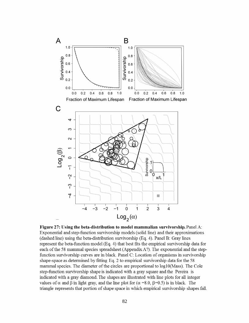
82

83
1% are predicted to exhibit r > 10. Using the Pereira approximation, approximately 21% of species are predicted to exhibit r > 3, while again, 1% are predicted to exhibit r > 10. Using the time-series approach, 7% of species are predicted to exhibit r > 3, with the maximum r estimate falling at r = 6.5. Figure 4 was limited by data availability, and thus compares r estimates across different data sets comprised of different species. However, for any given species with fixed life history traits, we find that the Cole estimate of r will always be larger than the time-series estimate of r which will be larger than the Pereira estimate of r.
∞ > 𝑟𝐶𝑜𝑙𝑒 ≥ 𝑟𝑡𝑖𝑚𝑒𝑠𝑒𝑟𝑖𝑒𝑠 ≥ 𝑟𝑃𝑒𝑟𝑒𝑖𝑟𝑎 > −∞ (4) The Cole approximation, arguably introduced as an algebraic convenience to the (then) computationally difficult Euler equation (Eq. 2), has been used and cited so broadly that its application has been effectively disconnected from the unrealistically harsh assumptions it makes about survivorship and reproduction. By reducing the estimation of a population’s growth rate from a life table to the far simpler problem of obtaining a few life history traits, the Cole approximation greatly broadens the range of species for which such growth rates may be calculated. However, the estimates obtained via this approximation are unreasonably large, especially for small bodied species (Fig. 2c). This is a result of unrealistic assumptions regarding both survivorship schedules and fecundity schedules.
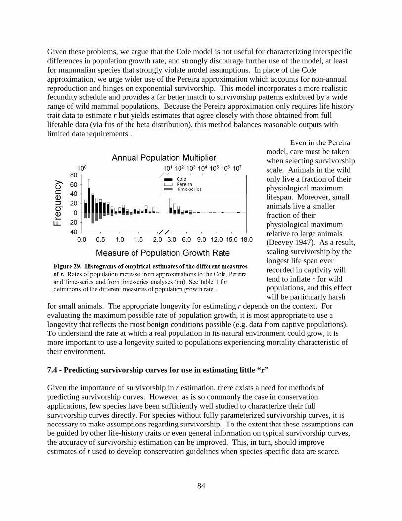
84
Given these problems, we argue that the Cole model is not useful for characterizing interspecific differences in population growth rate, and strongly discourage further use of the model, at least for mammalian species that strongly violate model assumptions. In place of the Cole approximation, we urge wider use of the Pereira approximation which accounts for non-annual reproduction and hinges on exponential survivorship. This model incorporates a more realistic fecundity schedule and provides a far better match to survivorship patterns exhibited by a wide range of wild mammal populations. Because the Pereira approximation only requires life history trait data to estimate r but yields estimates that agree closely with those obtained from full lifetable data (via fits of the beta distribution), this method balances reasonable outputs with limited data requirements .
Even in the Pereira model, care must be taken when selecting survivorship scale. Animals in the wild only live a fraction of their physiological maximum lifespan. Moreover, small animals live a smaller fraction of their physiological maximum relative to large animals (Deevey 1947). As a result, scaling survivorship by the longest life span ever recorded in captivity will tend to inflate r for wild populations, and this effect will be particularly harsh
for small animals. The appropriate longevity for estimating r depends on the context. For evaluating the maximum possible rate of population growth, it is most appropriate to use a longevity that reflects the most benign conditions possible (e.g. data from captive populations). To understand the rate at which a real population in its natural environment could grow, it is more important to use a longevity suited to populations experiencing mortality characteristic of their environment. 7.4 - Predicting survivorship curves for use in estimating little “r” Given the importance of survivorship in r estimation, there exists a need for methods of predicting survivorship curves. However, as is so commonly the case in conservation applications, few species have been sufficiently well studied to characterize their full survivorship curves directly. For species without fully parameterized survivorship curves, it is necessary to make assumptions regarding survivorship. To the extent that these assumptions can be guided by other life-history traits or even general information on typical survivorship curves, the accuracy of survivorship estimation can be improved. This, in turn, should improve estimates of r used to develop conservation guidelines when species-specific data are scarce.

85
In this element of our project, which appears in more detail as Appendix B of Lynch et al. 2011, our goal was to characterize the relationships between life history and trophic trait data (which are more readily available across species) with quantitative summaries of full survivorship schedules (which are scarce). In particular, we sought to understand how closely changes in the shape and scale of mammalian survivorship curves could be approximated by such traits as longevity, litter size, age to maturity, trophic level, and taxonomic group. 7.4.1 - Methods To relate survivorship shape to life history traits, we again turned to the beta distribution in Eq. 3. Specifically, we fit beta distribution survivorship curves to survivorship data for 37 captive mammals drawn primarily from International and Regional Studbooks kept by consortia of zoo biologists for the management of captive animal stocks. For this analysis, we selected species that represented the range of body sizes available in the database and included in our selection all those species for which wild population survivorship data sets were also available. To maximize data quality, we restricted our analysis to only those individuals in the database system on or after 1 January 1980. Particularly for the longest-lived species, survivorship data for the oldest age classes suffered from small sample sizes, thus we only considered those age classes represented by more than 10 individuals. After the small sample size age classes had been removed, a second level of filtering was done to ensure that the remaining survivorship curve represented the majority of the cohort mortality. Specifically, we only considered species for which the last recorded age class indicated less than 20% survival.
The (𝛼,𝛽) coordinates obtained from the fits of our beta distribution model (Eq. 3) to each captive animal survivorship curve were then plotted in shape space such that their locations could be compared. Again, the goal was to define a general region in shape space that captured the majority of captive mammalian survivorship curves. To define this region, we fit a bivariate normal distribution to the distribution of points in shape space. The resulting fitted distribution was also used to obtain estimates for the geometric means (across all species) of the two shape parameters. Finally, to determine which life history traits may be associated with survivorship shape, we used linear regression and principal components analysis (PCA) to look for correlations between life history traits such as body mass and litter size and the shape parameters 𝛼 and 𝛽.
In order to contrast wild survivorship curves with captive survivorship curves, we additionally fit our beta distribution model (Eq. 3) to 58 survivorship curves derived from field studies. We also directly compared 𝛼 and 𝛽 results for 7 species with survivorship curves in both the wild and captive animal databases (Note that two of the species with both wild and captive animal survivorship curves did not meet our criteria for inclusion in the previous analysis, but were included here due to the limited number of species for which both survivorship curves were available). Again, survivorship shape was visualized by plotting (𝛼,𝛽) coordinates in shape space. As before, the goal was to define a general region in shape space that captured the majority of wild mammalian survivorship curves. In addition, we wanted to compare the region in shape space associated with captive animal survivorship curves to the region in shape space associated with wild animal survivorship curves.

86
Finally, to relate our analysis of survivorship curves to r estimation for poorly studied species, we performed a leave-one-out cross-validation method based on estimated bounds in survivorship shape space. Specifically, we removed one focal species at a time from the data set. We then repeated (i.e. with the focal species missing) the bivariate fitting of a normal distribution to the points in shape space. From this fitted normal distribution we predicted the 50th percentile confidence envelope for the bounds on 𝛼 and 𝛽. Using this multispecies confidence envelope, we then calculated maximum and minimum r estimates for the focal species based on the Euler equation, species life history traits and the upper and lower bounds on survivorship shape. Sufficient life history information to calculate r was only available for 36 of the 37 species in our database. 7.4.2 - Results and Discussion Figure 30 shows the survivorship curve parameters displayed with summarizing information about their principle components (PC) and resulting curve shape. The geometric means of the two shape parameters were 𝛼 = 0.40 and 𝛽 = 0.86 respectively. In addition, we found that the distribution of shape parameter values was clustered along two principal axes that roughly corresponded to 𝛼/𝛽 (loosely interpreted as skew towards early vs. late mortality) and 𝛼𝛽 (loosely interpreted as unimodal vs. U-shaped mortality). While longevity, age to weaning and litter size were significantly correlated with the position of a species along the first principal component (PCA1) in shape space, we found no correspondingly strong covariate to explain variation along the second principal axis (PCA2). We also found no statistically significant relationship between the first principal component of life history and either principal component in shape space. We did, however, find a relationship between taxonomic group (specifically order) and survivorship shape. In fact, despite correlations between PCA1 and other life history traits, we found that variation along PCA1 is still best modeled by order alone. As was found in our previous

87
study, captive mammal survivorship shapes were largely contained within a triangle in shape space (Fig. 31).
Compared to captive animal survivorship curves, survivorship curves for wild animals are more variable, reflecting both the higher precision of the captive survivorship data and the integration of environmental factors with inherent drivers of survivorship in the wild. Moreover,
of the seven species for which both wild and captive animal survivorship curves were available, five showed a shift to smaller values of 𝛼 and 𝛽 when moving from the wild population to the captive population. This shift is associated with relatively higher juvenile mortality (compared to overall mortality) in the captive populations. Finally, with respect to predicting intrinsic growth rates, we found that r estimates for 28 of 36 species were bounded by the 50% confidence envelope for all species in the database. Furthermore, among those 28 species, leave-one-out cross-validation resulted in upper and lower limits on r that were, on average, only 22% above and 21% below the true value respectively. This finding emphasizes that not only are mammalian survivorship shapes quite similar across species, but that that similarity has an important functional consequence in terms of predicting population growth rates across species.
Despite all of the textbook dogma and subsequent discussion
regarding the three prototypical survivorship curves (types I, II and III), we find that all mammals in captivity have fairly similar survivorship curves most similar to type II survivorship curves but with varying degrees of type I character (high rates of mortality among the oldest age classes) and type III character (high rates of mortality among the earliest age classes). We find that survivorship shape is most closely correlated with life history traits relating to reproduction (relative age to weaning and gestation, litter size, litters per year, etc.). Our results explicitly reject the common textbook assertion that survivorship shape is related to body mass. Taxonomic order, however, was found to be the best predictor of survivorship shape, which is

88
consistent with earlier findings that suggest that order is significantly correlated with life history variation and annual survivorship. From a practical standpoint, it is useful to know what survivorship shapes can be expected among mammals. We have found that this is particularly true when using survivorship to estimate r for conservation planning. To this end, we believe that our method of defining bounds on survivorship shape based on a bivariate normal distribution will be extremely useful to practitioners of conservation ecology. In particular, our leave-one-out cross-validation shows that bounds on the normal distribution can be used to define upper and lower estimates on r that may be used as guidelines for management while more species-specific survivorship data are being collected. 7.5 - Conclusions
For conservation-related applications, it is important to consider the details of the organisms’ particular life-history characteristics to estimate maximum population growth rates accurately. In this respect, survivorship shape, survivorship scale and reproductive schedule are all important. The Cole approximation, which assumes step function survivorship and annual reproduction, will inflate r estimates under all circumstances. Management scenarios constructed using these inflated estimates will be inappropriate and potentially harmful. While it would be optimal to have empirically parameterized life-history traits for all species of conservation interest, we find that one “short-cut” between mammalian life-history traits and population growth rate is the less commonly used Pereira approximation. This model provides an unbiased estimate of r over the entire range of species sampled. We thus advocate its use, particularly when data limitations prevent less approximate methods (e.g. time-series analysis or empirically fitted survivorship functions). One approach for extending the accuracy of r estimation beyond what is possible from even the Pereira approximation is to incorporate more sophisticated, species-specific survivorship functions. We show that this may be possible using empirically defined general bounds on survivorship shape, as well as estimates of survivorship shape based on species traits, most notably order.

89
8. Part 6: Phylogenetic approaches for inferring recovery-related traits for poorly-studied species
8.1 - Background One of the main outcomes of this project is to expose the scale of data gaps that still exist in the literature related to conservation relevant species traits. Our sections on PVAs (Part 3) and estimating r (Part 5) have also shown how difficult it can be to do a rigorous job of estimating species traits, even when field data are available. When field data are not available, the problem is more difficult again. One possible way around a lack of field data is to infer trait characteristics for an unknown species based on what is known about a suite of well-studied species. Previously (Part 5), we showed that taxonomic order was an important predictor of survivorship. Given that survivorship is, itself, an important determinant of r, we suspected that related species may also share similar r values. This, in turn, suggested that r could be predicted even in the absence of any measured life-history traits.
Based on this hypothesis, we set out to determine if we could leverage information about phylogeny (species shared evolutionary histories) to predict values of r for poorly studied species based on known values for related species and information about phylogenetic structure. Here, we illustrate how focusing on phylogenetic relationships can be a more powerful predictive framework than using relationships between other traits, such as body mass. We took the approach that individual life history and ecological strategies are often phylogenetically structured (Webb et al. 2002). We viewed r as a synthetic life history trait that varies among species within a clade. This approach is warranted because inheritance from a common ancestor coupled with phylogenetic inertia routinely yields situations in which similar trait values cluster across related species (Jombart et al. 2010). Furthermore, it is exactly these types of relationships that, along with shared environmental factors, underpin the phylogenetic structuring of extinction risk and endangerment status across species (Heard and Mooers 2000; Purvis et al. 2000; Cardillo et al. 2008; Cooper et al. 2011). Using established phylogenies, we examined how successfully macroevolutionary models recover r values for well-studied species. We then leveraged phylogenetic relationships and suites of r values obtained for well-studied species to predict r for more poorly studied species, providing conservation practitioners with a means of estimating potential population growth rates of little-known species.
In order to develop and test these methods, we focused our efforts on two groups: mammals and birds. We selected mammals because we could build off of work that we did in the previous section (Part 5) and thus take advantage of the same datasets. Fortunately, the species in these datasets also had a well-resolved phylogeny that has already been worked out (Bininda-Emonds et al. 2008). We selected birds because they are another taxonomic group that has sufficient information to parameterize life history trait data and also had a phylogeny available for use. 8.1.1 - General approach We used phylogenetic independent contrasts (PIC) to predict values of r for extant species in the context of their shared evolutionary history (Felsenstein 1985; Garland et al. 1999;Garland and Ives 2000). This suite of techniques assumes a stochastic process model for trait evolution. In the simplest and most widely used form, the stochastic process is Brownian random motion,
90
where the variance parameter σ describes the scale of fluctuations in the unbiased random walk. Because r is fundamental to a species’ survival (e.g., it sets the upper bound on the rate at which a population can recover from low density), we expect it to evolve gradually rather than wildly, reflecting critical life history trade-offs such as longevity versus fecundity (Stearns 1989). For both the mammals and the birds, we considered two PIC models, one in which we considered only r (PIC-r) and the other where we included covariates (PIC-r with covariates). Details on including covariates are given separately in each section since we took different approaches.
Under either model, the phylogenetic position is known for each species whose value of r is to be predicted. In brief, we use the following procedure for each “unknown” species to be predicted. First, the tree is pruned to contain a single unknown species and all species with known r values. Second, the tree is temporarily rooted at the node immediately parental to the unknown tip species. Third, PIC is used to estimate r at this root. Finally, the root estimate is extended along the branch to the unknown tip. Under PIC-r, the expected value of r at the unknown tip is the same as at the temporary root. 8.1.2 - Model assessment For both birds and mammals we performed model assessment in two ways. First, we compared results of the two PIC processes against two null models. Second, we performed cross-validation procedures on all four alternative models. Two of these models were based on the PIC approach (PIC-r, and PIC-r with covariates) whereas the other two models represented null alternatives (Allometric null model, and Brownian motion null model). The null models were thus used as benchmarks against which to judge the predictive improvement provided by tree-based PIC models for r.
Allometric models for r require data on body mass but not on life history traits. These models have been used to explore interspecific relationships in r for decades (e.g., Cole, 1954; Blueweiss et al. 1978; Hennemann, 1984; Schmitz and Lavigne, 1984; Robinson and Redford, 1986; Ross 1992). Allometric approaches also feature prominently in metabolic scaling theory (e.g., (Savage et al. 2004). This foundation justifies our use of allometric-null models as alternatives to predictions based on PIC. Historically, allometric regression models did not attempt to account for phylogenetic non-independence among species in the datasets. However, phylogenetically based statistical approaches may be used in allometric analyses to incorporate covariation due to shared evolutionary history among species (Duncan et al., 2007; Fagan et al., 2010). This joint approach is most appropriate when building allometric models from existing databases which may be biased in their taxonomic representation (Fagan et al., 2010). Consequently, we used phylogenetically corrected least squares regression which accounts for correlated errors due to phylogenetic relatedness (Ives et al. 2007). Note that while our allometric-null models include phylogenetic information for the sample of species in the original analysis, they do not incorporate the phylogenetic position of species for which predicted values are sought. In other words, the allometric null regression models represent static mappings between female body size and r for the suite of species under consideration whereas the PIC models customize predictions for the target species based additionally on their shared evolutionary history with the rest of the clade (Garland and Ives 2000).
The Brownian motion null model incorporates neither body mass nor phylogenetic information. In this model, observed r values are treated as independent samples from a normal distribution, for which the mean and variance are estimated from the known species in the clade.

91
This model is equivalent to the Brownian motion model of r evolution used by the PIC-r model, but on a star-shaped rather than bifurcating phylogenetic tree.
We used leave-one-out cross-validation to test model performance. For each species with a known r value, taken one at a time, this value was ignored and the species was treated as “unknown” in the prediction procedure. This was carried out for both PIC models. Model performance was assessed in three ways. First, we assessed general agreement of the predicted, (�̂�) and observed (𝑟) values by examining the relationship between �̂�and 𝑟 for each group of species. Second, we assessed accuracy by comparing proportion prediction errors, computed as for each species. This second method was performed for all four alternative models and gave us a means of comparing the performance of the PIC methods as compared to the null models. Third, we assessed accuracy for both PIC-r and PIC-r-mass models by scoring the proportion of species for which the 95% prediction intervals of the model included the observed r values. 8.2 - Mammal implementation: developing the method To develop and test our phylogenetic comparative method for r estimation, we considered two different clades of mammals: the suborder Caniformia (which includes the dog, bear, skunk, weasel, raccoon, seal, and sea lion families) and the family Cervidae (the true deer). Both of these clades have well studied phylogenies (though the phylogeny for Cervidae is not as well resolved), which is a requirement for our approach. In contrast, whereas there is a wealth of life history data for r estimation in Caniformia, r estimates for Cervidae are more sparsely available. By considering both clades, we were able to test our approach in two different contexts with respect to level of clade characterization. We obtained the molecular (cytB), species-level phylogeny of the order Carnivora (parent to the Caniformia) from Agnarsson et al. (2010) and smoothed it to an ultrametric tree using the R function chronopl (Sanderson 2002). We used a lower-resolution phylogeny for Cervidae, extracted from the Bininda-Emonds et al. (2008) mammalian supertree in an already ultrametric form.
Values of r for well-studied species within each clade were established based on the Pereira approximation to the Euler equation in combination with life history trait data obtained from published compilations (Walker et al. 1983; Ernest 2003; Jones et al. 2009). As discussed in Part 5, the Pereira approximation to Eq. 1 assumes Type II (exponential) survivorship and allows for episodic, pulsed reproduction rather than continuous reproduction (Pereira 2006). Both of these biologically realistic modifications are especially appropriate for mammalian life history. Under these assumptions, Eq. 1 becomes
( ) 10 0
)( =
−∆−∫ ∑∞ ∞
=
+− dxeyxmy
xr µβδ , (5)
where r is the maximum population growth rate, m is the maximum number of female offspring per reproductive episode (litter), ∆ is the average interval between litters, β is the minimum age of first reproduction, and µ is the average mortality rate. δ(z) is an interval delta function that equals 1/T for 0 < z < T and is zero otherwise, where T is the duration of the mammalian “birth pulse,” which is taken to be one day (Pereira 2006). This model does not constrain reproduction to occur on an annual basis but does assume constant fecundity per birth event. The integral and sum in Eq. 5 can be evaluated, yielding

92
( )( )( ) 111 )(
)(
)(
=−−
++−
∆+−
+−βµ
µ
µ
µr
r
Tr
eee
Trm
. (6)
This work was published at Proceedings of the Royal Society B: Biological Sciences (Appendix 2). 8.2.1 - Results and Discussion Overall, the phylogenetic (PIC) methods are successfully able to recover unknown r values. Leave-one-out cross-validation predictions from the PIC-r and PIC-r-mass models showed good general agreement with life history trait based estimates of r for both the Caniformia and the Cervidae (Fig. 32). In the Caniformia, prediction errors from PIC-r were distributed roughly equally around a 1:1 line of correspondence with two exceptions, a diverse group of species with
small-medium observed values of r (which were overestimated) and two species of weasels with very large observed values of r (which were under estimated). Overall, for both taxa, both the
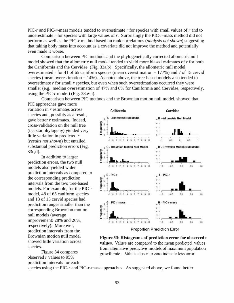
93
PIC-r and PIC-r-mass models tended to overestimate r for species with small values of r and to underestimate r for species with large values of r. Surprisingly the PIC-r-mass method did not perform as well as the PIC-r method based on rank correlations (analysis not shown) suggesting that taking body mass into account as a covariate did not improve the method and potentially even made it worse.
Comparison between PIC methods and the phylogenetically corrected allometric null model showed that the allometric null model tended to yield more biased estimates of r for both the Caniformia and the Cervidae (Fig. 33a,b). Specifically, the allometric null model overestimated r for 41 of 65 caniform species (mean overestimation = 177%) and 7 of 15 cervid species (mean overestimation = 14%). As noted above, the tree-based models also tended to overestimate r for small r species, but even when such overestimations occurred they were smaller (e.g., median overestimation of 47% and 6% for Caniformia and Cervidae, respectively, using the PIC-r model) (Fig. 33.e-h).
Comparison between PIC methods and the Brownian motion null model, showed that PIC approaches gave more variation in r estimates across species and, possibly as a result, gave better r estimates. Indeed, cross-validation on the null tree (i.e. star phylogeny) yielded very little variation in predicted r (results not shown) but entailed substantial prediction errors (Fig. 33c,d).
In addition to larger prediction errors, the two null models also yielded wider prediction intervals as compared to the corresponding prediction intervals from the two tree-based models. For example, for the PIC-r model, 48 of 65 caniform species and 13 of 15 cervid species had prediction ranges smaller than the corresponding Brownian motion null models (average improvement: 28% and 26%, respectively). Moreover, prediction intervals from the Brownian motion null model showed little variation across species.
Figure 34 compares observed r values to 95% prediction intervals for each species using the PIC-r and PIC-r-mass approaches. As suggested above, we found better

94
performance by the simple PIC-r model of trait evolution than by the more complex PIC-r-mass model that included mass as a covariate.
In fact, for the Caniformia, PIC-r-mass actually yielded worse predictions (median prediction error was 48% larger with PIC-r-mass). We fully expected the PIC-r-mass model to improve upon the results from the simpler PIC-r model by including extra information about how species differed from one another. The lack of improvement that we observed may stem from the largely similar performance of the PIC-r model across species, irrespective of differences in body mass; indeed, we found no correlation between prediction error and mass for either the Caniformia or the Cervidae. These results echo findings in Part 5 where biomass was not a good predictor of mammalian survivorship, but other traits, such as trophic level and diet were.
Both the PIC-r model and the PIC-r-mass model gave large 95% prediction intervals (Fig. 34). However, the observed values for 83-86% and 73% of caniform and cervid species, respectively, fell within one standard error of the predicted mean. Prediction intervals were smaller for the PIC-r-mass model than for the PIC-r model in 59 of 61 species-wise comparisons in the Caniformia, shrinking by an average of 9.8%. In order to visualize the

95
relationship between phylogeny and values of r, we plotted PIC-r results on phylogenetic trees for Califormia (Fig. 35a) and Cervidae (Fig. 35b).
Given the interdependencies among life history traits and population growth we suspected that some improvement on these PIC approaches may be possible by incorporating life history traits other than body mass as covariates of the evolutionary model. This is discussed in the following section, using shorebirds as a focal group. Specifically, we included egg size and body size in our modeling efforts. Other traits such as age at first reproduction or average litter size are known to covary with measures of population growth rate across diverse species (Saether and Bakke 2000); (Heppell et al. 2000). Those covariates could also be included in our macroevolutionary models and might sharpen predictions of how r evolves across species. The potential importance of such a future extension is made clear by the cross-validation errors that occurred in isolated cases where certain species had r estimates much different than their neighbors on the phylogeny. For example, compared to closely related species, the short-tailed and least weasels Mustela erminea and M. nivalis (Caniformia: Mustelidae) had unusually large r values that were driven largely by young ages at first reproduction (e.g., females of these species are often mated before being weaned (Harris and Yalden 2008) (Fig. 34a).

96
8.3 - Shorebird implementation We next implemented our basic PIC method for estimating r on a new group of animals, shorebirds (Charadriiformes). Charadriiformes is a large order of birds that has been well studied on both ecological and evolutionary fronts and for which we have reasonable phylogenetic resolution. By focusing on this group, we were able to accomplish three goals. First, we were able to determine if PIC-r methods of estimation could be successfully applied to another group with very different life history traits. Second, we were able to determine if using different life history traits other than body mass would improve predictions. Third, we were able to explore the effect of treating body mass as an evolvable trait, rather than a static covariate. This last goal was motivated by our finding that treating body mass as static covariates did not improve predictions (and sometimes even made them worse) for our mammalian data set.
Rather than treating body mass as a static covariate, another take on the problem recognizes that mass, as well as r, can evolve over time. If one treats both r and other traits as evolvable entities, different results may emerge than if all traits (except r) are viewed as static covariates. Here, we considered a PIC-covariates model where female body mass and/or egg mass are additionally included as evolvable covariates. Egg mass was chosen as a second covariate because it varies widely across bird species, and is a key life history trait that, though related to per-capita reproductive output (Williams 1994), does not enter the Euler equation directly.
Values of r for well-studied species within each clade were again based on an approximation to the Euler equation. However, since bird biology is distinct from mammal biology, a different approximation was used. In this case, we assumed an approximation found in Pereira et al. (2004) that specifically accommodates bird reproductive ecology – hereafter referred to as ‘Pereira-Bird’. The ‘Pereira-Bird’ equation predicts r based on broods per year, eggs per clutch and mortality rate where, again, exponential survivorship is assumed.
We obtained the species-level shorebird supertree necessary to perform PIC from Thomas et al (2004) and smoothed it to an ultrametric tree using the R function chronopl (Sanderson 2002). To understand where and in what phylogenetic context it is possible to leverage data about well-studied species to infer r for poorly studied species, we considered shorebird clades at three hierarchical levels of organization within shorebird phylogeny. These were 1) the supertree as a whole, 2) the supertree broken into three major clades consisting of the suborders Charadrii + Chionidi, Lari, and Scolopaci + Thinocori, and 3) four major families within the Charadriiformes, namely the Alcidae, Charadriidae, Laridae and Scolopacidae. Again we studied several different PIC models and counterpart null models. The PIC models we considered were: 1) the basic PIC-r model, where r for an unknown species is predicted using only values of r for known species and the phylogeny of the clade; 2) a PIC-r-mass model where both mass and r are allowed to evolve on the phylogeny; and 3) a PIC-r-egg mass model where both egg mass and r are allowed to evolve on the phylogeny. Following the same approach that was taken with the mammalian data set, model validation and assessment was performed using leave-one-out cross validation and comparison to allometric and Brownian motion null models. The work described here is still in preparation for submission.

97
8.3.1 - Results and Discussion
Figure 36 shows percent prediction error for both the null models (Allometric and Brownian) and the phylogenetic models (PIC-r and PIC-r-covariate) at the three different taxonomic hierarchical levels (Order, Clade, Family). Both null models performed reasonably well when applied at the family level. However, extending the null models to broader phylogenetic scales resulted in large errors (Fig. 36). For example, using the allometric null

98
model, maximum proportional prediction error was less than 15× the observed r value for analyses of individual families, but over 40× the observed r value for analyses of the entire shorebird clade. In this regard, the PIC approa7ch offered a substantial improvement. Compared to the Brownian motion null model, PIC-r provided more accurate estimates of r for the shorebird group as a whole (median prediction error improved by 27%) and for the three major clades (by 8% for the Charadrii + Chionidi, 18% for the Lari, and an impressive 49% for the Scolopaci + Thinocori). It did not, however, generally improve model performance at the family level (Fig. 36). Our analysis suggests that phylogenetic structure is not that important in the evolution of r in the local context of closely related species, but that phylogenetic relationships can improve our understanding of the evolution of r at higher taxonomic levels that incorporate more diversification among species. Similar to what was found for mammals, the PIC models for birds that incorporated covariates did not consistently improve prediction accuracy (Fig. 37). Moreover, although the PIC-r-covariates models did yield smaller confidence intervals than the simple PIC-r models, these confidence intervals less frequently captured the actual observed r

99
values Fig. 37). For instance, under PIC-r, one standard error encompassed the true value of r for 75% of species. In contrast, under the PIC-r-mass, PIC-r-eggmass and PIC-r-mass-eggmass models one standard error encompassed the true value of r for 67%, 65% and 59% of species
respectively. Therefore, while the phylogenetically structured PIC model was beneficial for predicting population growth potential, there was no overall benefit to incorporating additional life history information in the form of model covariates. One reason that the model with covariates may not have performed well is because there was an overall negative relationship

100
between r and the two traits that we included (body size and egg mass), although the two traits did correlate quite strongly with each other (results not shown). In order to visualize the relationship between phylogeny and values of r, in Figure 38 we plotted PIC-r on phylogenetic trees. Overall, the various PIC models offered substantial improvements over the null models – especially the allometric null model. Particularly the PIC-r model without covariates reduced mean and median prediction errors relative to the null models. These improvements were most substantial when applied at the scale of broad phylogenetic datasets (i.e., Order and Clade levels) (Fig. 36). In contrast, PIC-r approaches did not lead to consistent improvements in estimates of r when analyses were performed at the family level. Specifically, although family-level PIC predictions offered improvements over the allometric null model, they did not improve upon the Brownian motion null models for all families. This series of results appears strongly linked to data density and sample size issues for the different phylogenies on which the PIC inferences were conducted. More data, even if it is from distant evolutionary relatives, proved useful in accurately predicting r across the entire group of species. However, a lack of statistically informative heterogeneity in r among closely related species meant that the improvement afforded by the PIC-r model relative to the null model was reduced in small lineages. 8.4 - Conclusions Knowledge of species’ potential population growth rates is critical for understanding population dynamics and informed conservation decision-making and management (Mace and Lande 1991). Because of this, recent efforts have sought to estimate various population growth rate parameters using demographic traits in concert with other approaches such as allometric regressions (Saether and Bakke 2000; Hone et al. 2010; Pereira and Daily 2006). In contrast, our approach took advantage of the shared evolutionary history among species to predict potential population growth rates, and it performed well even when only limited life history data were available to inform the predictions. The tree-based methods we adopted routinely yielded credible predictions within each of two dissimilar mammalian groups and a large clade of birds, thereby providing a substantial improvement over traditional null models (Fig. 33, 36). Indeed, even application of the modeling approach to the small, low diversity cervid clade showed that our approach was robust to both limited observed r data and incomplete phylogenetic resolution, two problems that are likely to appear in other taxa.
By leveraging data from better known species to inform understanding of poorly known species, our application of phylogenetic comparative methods to the problem of population growth rate estimation fills a crucial gap in the toolkit of quantitative conservation biology. In particular, we have provided conservation practitioners with a method for predicting species’ capacities for population growth even when no species-specific trait data are available. Without the appropriate suite of life history trait data, it is not possible to parameterize equations to estimate r. In times past, this would leave conservation practitioners without much guidance as to that species’ capacity for population growth or recovery (but see Heppell et al. 2000 for a discussion of intercorrelations among mammalian life history traits and their utilities in predicting elasticities in population growth rate using demographic matrix data). In contrast, with the phylogenetic comparative approaches implemented here, researchers can estimate r for poorly known species reasonably accurately, and with an assessment of uncertainty.

101
Estimating maximum per capita population growth rates via tree-based prediction methods may be especially advantageous to conservation planners who are seeking ways of comparing species with regard to their needs or risks. For example, in landscape-specific comparisons across several species, information on r, whether observed or predicted, may be viewed as an index of species’ vulnerabilities to extinction processes due to a common threat (Fagan et al. 2001; Cortes 2002). The strong agreement that we find between observed r and predicted �̂� (e.g. Fig. 32) highlights the potential utility of our PIC approach for prioritization efforts that span multiple species. In particular, the strong rank agreement that we observe offers planners reassurance that species predicted to be especially vulnerable because they have low r will actually have low maximum population growth rates compared to other species. Ranking species’ vulnerabilities using phylogenetically predicted estimates of r would be most useful in data-poor situations where a suite of species faces a common external threat as opposed to the (much rarer) data-rich situations in which formal assessments of extinction risk via population viability analyses are possible.
Beyond conservation-relevant results, our efforts have the additional benefit of introducing a joint empirical-theoretical framework for explicitly modeling key aspects of the ‘ecogenetic loop’ that links life history traits, demography, and evolution (Partridge and Harvey 1988; Kokko and Lopez-Sepulcre 2007; Coulson et al. 2010). Specifically, future work could compare how well these macroevolutionary models perform for various life history quantities, such as those appearing in variants of the Euler equation, both relative to one another, and relative to r as a synthetic life history trait. Continued development of evolutionary models for r and other life history traits across species should yield insights into the limits of demographic plasticity across species and, at the same time, increase our understanding of species resilience (Reed et al. 2010).
Another future direction would be to include more complex models of character evolution. In particular, a complicating factor not accounted for in our analysis is the potential effect of r on extinction or speciation rates. Population growth rates have previously been used as a proxy for evolutionary fitness and have been implicated as potential drivers of diversity (Huston 1979; Geritz et al. 1997) and diversification rate (Liou and Price 1994). Several mechanisms may contribute to this linkage between population growth rates and diversification, but a key one is that species with low maximum per capita population growth rates are less able to recover from low population size and may therefore be more prone to extinction, which would increase extinction rates on trees dominated by slow-growing, ‘low r’ species. A similarly key issue is that correlations between r, generation time, and rates of molecular evolution (Blueweiss et al. 1978; Martin and Palumbi 1993; Smith and Donoghue 2008) may lead to association between r and speciation rate, with ‘high r’ lineages speciating more rapidly. Effects of traits on diversification rate are not naturally incorporated in the PIC framework. However, a recent phylogenetic model of the evolution of a continuously valued character that affects diversification (FitzJohn 2010) presents an alternative approach. This model, when coupled with detailed phylogenetic data, extensive data on r values, and potentially covariates, may be useful for disentangling the effects of population growth rate on speciation and extinction rates.

102
9. CONCLUSIONS AND IMPLICATIONS FOR FUTURE RESEARCH
Overall, our ultimate goals of identifying sufficient similarities among species such that we could accurately cross-predict recovery goals proved elusive. Difficulties derived from several sources including: 1) gaps in the database of species-specific traits and threats that persisted despite herculean efforts to consolidate available information; 2) unexpected sensitivity in interspecific proximity metrics to heterogeneity in data availability; 3) relationships between the number of individuals (or number of populations or area of extent) known to exist at different times prior to listing and the recovery goals themselves; and 4) biological and/or contextual idiosyncrasies of the listed species themselves that reduced opportunities for identifying similarities among species.
Nevertheless, we were successful in several key areas. For example, we made good progress in characterizing when and where PVA approaches are most utilized and most informative in conservation efforts for TES species (PVA analyses in Part 3). Moreover, we were able to demonstrate the broad utility of simple, generic models for predicting quasi-extinction dynamics across a broad range of species (CSEG model in Part 3). Likewise, we are pleased with our successful efforts to employ the statistical method of phylogenetically independent contrasts to infer population growth rate and other traits for little known species (Parts 5 and 6). Going forward, there are several situations in which the general concept of leveraging data from well-studied species to inform conservation and management decisions for poorly known species may prove profitable. For example, further development of the phylogenetic approaches for predicting r seems warranted. In addition, there may be an opportunity to bring together elements of several of the approaches that we have already explored in a new context that could be useful for selected species.
9.1 - Further development of phylogenetic approaches
Even with sparse life history data, the simplest ‘base model’ was able to estimate r
accurately while also maintaining strong rank agreement in r values among species. Because a listed species’ r is indicative of its ability to recover from small population sizes when extrinsic threats are ameliorated (or held constant across species in comparative analyses), refinements in our ability to estimate r could aid ranking of species with respect to conservation priorities. For example, species with the smallest r values would be those most jeopardized by small population sizes, because once reduced to low abundance, such species would take the longest time to increase. Likewise, a ‘low r’ species would, on average, be expected to reside on the endangered species list for a longer period of time than would a high r species with the same recovery goal. Such differences in potential “list-residence time” could clearly feedback into decisions about species management and resource allocation. Given these potential linkages to management, techniques for estimating r could be developed building on our findings thus far. For example, improved PIC approaches may be possible using non-mass traits as covariates of the evolutionary model. That is, even if we lack sufficient life history data to calculate r for one of the poorly known species, we may have data on one or more of the life history parameters that enter Eq. 2-3. Traits such as age at first reproduction or average litter size covary with measures of population growth rate across diverse species (Saether and Bakke 2000, Heppell et al. 2000), and including them as covariates in our macroevolutionary models might sharpen predictions of how r evolves across species.
103
9.2 - Establishing defensible recovery criteria
Neel and Che-Castaldo are pursuing an alternative path forward to overcome the key obstacles identified through the SERDP funded research that will provide a means of establishing defensible recovery criteria even in the face of data gaps. The primary need we identified is increased understanding of links between the general theoretical risks facing small and declining populations and the risks associated with abundances specified for recovery. Lack of ability to link particular abundances with probability of persistence hinders objective evaluation of existing recovery criteria or development of new criteria. Thus, although variation in numerical abundances specified as recovery criteria has caused criticism, there is, in fact, currently no scientific basis to say that the variation is truly problematic. Given wide interspecific variation in threat context and underlying biology, even substantial differences in the numbers of populations and individuals required for recovery could correspond to broadly similar extinction risks across species. Translating criteria into the common currency of extinction risk would allow more transparent assessment of whether or not specified abundance measures and threat abatement would be sufficient to ensure sufficient probability of long-term persistence to leave species ‘not in need of the provisions of the Act’.
Thus, we suggest fundamentally improving recovery criteria requires a means of rigorously quantifying extinction risk that would result from attainment of specified criteria, including both numerical abundance and abatement of threats. By integrating risks due to both intrinsic and extrinsic factors and the interactions between them (Lee and Jetz 2011), the approach we are developing would address risk associated with specific abundances and trends as they are modified by the threat context in which species are embedded (Isaac and Cowlishaw 2004). This approach will allow fair and unbiased evaluation of recovery criteria across species.
We also suggest that improving recovery requires integrating more quantitative criteria for habitat and range extent that can complement demographic values for populations and individuals. The results of our investigations of traditional PVA analysis in combination with conclusion of others indicates they are not appropriate for setting quantitative recovery criteria. However, our research highlighted the fact that quantitative measures of these aspects of abundance other than individuals and populations are most often missing from recovery plans. Thus, despite the fact that change in distribution and extent are major factors in determining extinction risk, and habitat protection is a primary recovery action, habitat or range amounts are rarely treated explicitly or quantitatively in recovery plans. Establishing objective and measurable criteria for habitat and range would improve the likelihood of such conservation and increase the potential that species will be maintained at levels sufficient for ecological functioning and adaptation to future environmental conditions that are essential for long-term prevention of extinction. We have research efforts under way to better quantify changes in habitat availability and to translate those changes into extinction risk.
Being able to compare given a species’ abundance, biology and the threat context in which it is situated is critical to comparing recovery criteria across species. Determining incremental changes in risk as a function of threat abatement is particularly difficult and to date no scientifically based methodology exists to meet this need. Our goal over the next 1-3 years is to develop such a methodology. This methodology will integrate the objective and measurable abundance criteria for individuals, population, range and habitat availability with the ongoing threat context in which the species exists to develop quantify a change in extinction risk. We have been working with the US Fish and Wildlife Service on these efforts since early 2012 and

104
will continue to do so. Short of a formal methodology, more explicit articulation of the general logic for requiring particular abundance values and links between these abundances and reduction of particular threats would vastly improve recovery plans. 9.3 - Future synthetic efforts
Taken together, our partial success in several areas suggests an opportunity for a
composite approach that might prove useful in the development of recovery goals for poorly known species. Specifically, there seems to be an opportunity to combine the primary strength of the comparison set approach with the primary strength of the phylogenetic approach. To see this, note that when the comparison set worked well, it was able to identify a suite of species that, by virtue of similar traits and threats, exhibited variations in population size similar to those of a focal species (Fig. 22); that is, ‘similarity in variability of population change.’ In contrast, the comparison set approach proved unable to accurately recover mean rates of population growth or decline. However, the phylogenetic approach leveraged what was known about species’ shared evolutionary histories to estimate a focal species’ baseline rate of population growth. Although the intrinsic rate of increase (r) estimated by the phylogenetic approach is not the same statistical measure as the mean rate of growth (µ) estimated via the diffusion approximation, the two measures are related and often similar in magnitude. Thus, there may be an interesting opportunity to combine these two sources of information about a focal species in the service of its conservation, such as by calculating a recovery goal that reflects both the species intrinsic capacity for growth and the severity of population fluctuations that the focal species is likely to experience. The details of this merged approach would need to be worked out, and of course it would not be useful for those species where we were unable to identify stable comparison sets, but it does seem worthy of exploration. 9.4 - Final thoughts
Overall, the results presented here highlight both successes and shortcomings of our efforts to leverage data from well-studied species to inform recovery efforts for poorly known species. Clearly, the lack of predictive certainty that our approaches afforded on a case-by-case basis is disappointing (Part 4). However, the broad utility of simple, generic models for predicting quasi-extinction dynamics across a broad range of species (CSEG model in Part 3) and the exciting opportunities afforded by phylogenetic of population growth rate (Parts 5 and 6) are reasons for optimism.
Conservation biology is increasingly adopting multiple approaches to conservation, some traditional single-species, some attempting to integrate efforts for multiple species. Taking a multispecies perspective, a view that is necessitated both by the increasing numbers of species of conservation concern and by the general need to act quickly to halt or reverse population declines, presents many challenges. Often such action must take place in the absence of solid information on each component species, and from a practical perspective, broad brush multispecies conservation efforts may trade off case-by-case certainty for time. Although the knowledge that we will guess right “on average” may provide little solace when particular species or populations fail to persist, we must keep in mind that real species are, by definition, unique biological entities for some (potentially high) degree of specialized, idiosyncratic conservation efforts may be necessary.

105
10. Literature Cited Agnarsson, I., M. Kuntner, and L. J. May-Collado. 2010. Dogs, cats, and kin: A molecular
species-level phylogeny of Carnivora. Molecular Phylogenetics and Evolution 54:726-745.
Akcakaya, H. R. and P. S. Sjӧgren-Gulve. 2000. Population viability analysis in conservation biology: An overview. Ecological Bulletins:9-21.
Andelman, S. J. and W. F. Fagan. 2000. Umbrellas and flagships: Efficient conservation surrogates or expensive mistakes? Proceedings of the National Academy of Sciences of the United States of America 97:5954-5959.
Beissinger, S. R. 2002. Population viability analysis: past, present, and future.in S. R. Beissinger and D. McCullough, editors. Population Viability Analysis. University of Chicago Press, Chicago, IL.
Beissinger, S. R. and M. I. Westphal. 1998. On the use of demographic models of population viability in endangered species management. Journal of Wildlife Management 62:821-841.
Bevill, R. L. and S. M. Louda. 1999. Comparisons of related rare and common species in the study of plant rarity. Conservation Biology 13:493-498.
Bininda-Emonds, O. R. P., M. Cardillo, K. E. Jones, R. D. E. MacPhee, R. M. D. Beck, R. Grenyer, S. A. Price, R. A. Vos, J. L. Gittleman, and A. Purvis. 2008. The delayed rise of present-day mammals (vol 446, pg 507, 2007). Nature 456:274-274.
Blackburn, T. M. and K. J. Gaston. 2002. Extrinsic factors and the population sizes of threatened birds. Ecology Letters 5:568-576.
Blueweiss, L., H. Fox, V. Kudzma, D. Nakashima, R. Peters, and S. Sams. 1978. Relationships between body size and some life-history parameters. Oecologia 37:257-272.
Bocetti, C.i., D.D. Goble, and J. M. Scott. 2012. Using Conservation Management Agreements to Secure Postrecovery Perpetuation of Conservation-Reliant Species: The Kirtland’s Warbler as a Case Study. BioScience 62: 874-879
Boyce, M. S. 1992. Population viability analysis. Annual Review of Ecology and Systematics 23:481-506.
Breiman, L. 2001. Random forests. Machine Learning 45:5-32. Breiman, L., J. H. Friedman, R. A. Olshen, and C. J. Stone. 1984. Classification and Regression
Trees. Wadsworth and Brooks, Pacific Grove, CA. Brook, B. W., J. J. O'Grady, A. P. Chapman, M. A. Burgman, H. R. Akcakaya, and R.
Frankham. 2000. Predictive accuracy of population viability analysis in conservation biology. Nature 404:385-387.
Brook, B. W., N. S. Sodhi, and C. J. A. Bradshaw. 2008. Synergies among extinction drivers under global change. Trends in Ecology & Evolution 23:453-460.
Brooks, T., A. Balmford, N. Burgess, L. A. Hansen, J. Moore, C. Rahbek, P. Williams, L. A. Bennun, A. Byaruhanga, P. Kasoma, P. Njoroge, D. Pomeroy, and M. Wondafrash. 2001. Conservation priorities for birds and biodiversity: do East African Important Bird Areas represent species diversity in other terrestrial vertebrate groups? Ostrich:3-12.
Brown, J. H., J. F. Gillooly, A. P. Allen, V. M. Savage, and G. B. West. 2004. Toward a metabolic theory of ecology. Ecology 85:1771-1789.

106
Calder, W. A. 2000a. Diversity and convergence: scaling for conservation. Pages 297-323 in J. H. Brown, West, G.B., editor. Scaling in biology. Oxford University Press, New York, New York, USA.
Calder, W. A. 2000b. Diversity and convergence: scaling for conservation.in J. H. Brown and G. B. West, editors. Scaling in Biology. Oxford University Press, New York, NY.
Campbell, F. 1991. Endangered plant species shortchanged: Increased funding needed. Endangered Species Update 9:6.
Cardillo, M., G. M. Mace, J. L. Gittleman, K. E. Jones, J. Bielby, and A. Purvis. 2008. The predictability of extinction: biological and external correlates of decline in mammals. Proceedings of the Royal Society B-Biological Sciences 275:1441-1448.
Caro, T., J. Eadie, and A. Sih. 2005. Use of substitute species in conservation biology. Conservation Biology 19:1821-1826.
Caro, T. M. and G. O'Doherty. 1999. On the use of surrogate species in conservation biology. Conservation Biology 13:805-814.
Caughley, G. 1994. Directions in conservation biology. Journal of Animal Ecology 63:215-244. Channell, R. and M. V. Lomolino. 2000. Trajectories to extinction: spatial dynamics of the
contraction of geographical ranges. Journal of Biogeography 27:169-179. Chase, M. K., W. B. Kristan, A. J. Lynam, M. V. Price, and J. T. Rotenberry. 2000. Single
species as indicators of species richness and composition in California coastal sage scrub birds and small mammals. Conservation Biology 14:474-487.
Che-Castaldo, J., and D. Inouye. 2011. The effects of dataset length and mast seeding on the demography of Frsera speciosa, a long-lived monocarpic plant. Ecosphere 2:article 126.
Clark, J. A., J. M. Hoekstra, P. D. Boersma, and P. Kareiva. 2002. Improving U.S. Endangered Species Act recovery plans: Key findings and recommendations of the SCB recovery plan project. Conservation Biology 16:1510-1519.
Cole, L. C. 1954a. The Population Consequences of Life History Phenomena. The Quarterly Review of Biology 29:103-137.
Cole, L. C. 1954b. The population consequences of life history phenomena. Quarterly Review of Biology 29:103-137.
Cooper, N., R. P. Freckleton, and W. Jetz. 2011. Phylogenetic conservatism of environmental niches in mammals. Proceedings of the Royal Society B-Biological Sciences 278:2384-2391.
Cortes, E. 2002. Incorporating uncertainty into demographic modeling: Application to shark populations and their conservation. Conservation Biology 16:1048-1062.
Coulson, T., G. M. Mace, E. Hudson, and H. Possingham. 2001. The use and abuse of population viability analysis. Trends in Ecology & Evolution 16:219-221.
Coulson, T., S. Tuljapurkar, and D. Z. Childs. 2010. Using evolutionary demography to link life history theory, quantitative genetics and population ecology. Journal of Animal Ecology 79:1226-1240.
Courchamp, F., B. Grenfell, and T. Clutton-Brock. 1999. Population dynamics of obligate cooperators. Proceedings of the Royal Society B-Biological Sciences 266:557-563.
Crone, E. E., E. S. Menges, M. M. Ellis, T. Bell, P. Bierzychudek, J. Ehrlen, T. N. Kaye, T. M. Knight, P. Lesica, W. F. Morris, G. Oostermeijer, P. F. Quintana-Ascencio, A. Stanley, T. Ticktin, T. Valverde, and J. L. Williams. 2011. How do plant ecologists use matrix population models? Ecology Letters 14:1-8.

107
Crouse DT, Crowder LB, Caswell H. 1987. A Stage-Based Population-Model for Loggerhead Sea-Turtles and Implications for Conservation. Ecology 68 (5): 1412-1423
Cushman, S. A., K. S. McKelvey, B. R. Noon, and K. McGarigal. 2010. Use of Abundance of One Species as a Surrogate for Abundance of Others. Conservation Biology 24:830-840.
Deevey, E. S., Jr. 1947. Life Tables for Natural Populations of Animals. The Quarterly Review of Biology 22:283-314.
DeMaster, D., R. Angliss, J. Cochrane, P. Mace, R. Merrick, M. Miller, and e. al. 2004. Recommendations to NOAA Fisheries: ESA Listing Criteria by the Quantitative Working Group. NOAA Tech. Memo. NMFS-F/ SPO-67. U.S. Department of Commerce, Washington, DC.
Denney, N. H., S. Jennings, and J. D. Reynolds. 2002. Life–history correlates of maximum population growth rates in marine fishes. Proceedings of the Royal Society of London. Series B: Biological Sciences 269:2229-2237.
Dennis, B., P. L. Munholland, and J. M. Scott. 1991. Estimation of growth and extinction parameters for endangered species. Ecological Monographs 61:115-143.
Doak, D., D. Thomson, and E. Jules. 2002. Population viability analysis for plants: Understanding the demographic consequences of seed banks for population health.in S. R. Beissinger and D. McCullough, editors. Population Viability Analysis. University of Chicago Press, Chicago, IL.
Doak, D. F., K. Gross, and W. F. Morris. 2005. Understanding and predicting the effects of sparse data on demographic analyses. Ecology 86:1154-1163.
Dobson, A. P., J. P. Rodriguez, W. M. Roberts, and D. S. Wilcove. 1997. Geographic distribution of endangered species in the United States. Science 275:550-553.
Duncan, R. P., D. M. Forsyth, and J. Hone. 2007a. Testing the Metabolic Theory of Ecology: Allometric Scaling Exponents in Mammals. Ecology 88:324-333.
Duncan, R. P., D. M. Forsyth, and J. Hone. 2007b. Testing the metabolic theory of ecology: Allometric scaling exponents in mammals. Ecology 88:324-333.
Ellner, S. P., J. Fieberg, D. Ludwig, and C. Wilcox. 2002. Precision of population viability analysis. Conservation Biology 16:258-261.
Ellstrand, N. C. and D. R. Elam. 1993. Population genetic consequences of small population-size - implications for plant conservation. Annual Review of Ecology and Systematics 24:217-242.
Elphick, C. S., J. M. Reed, and J. M. Bonta. 2001. Correlates of population recovery goals in endangered birds. Conservation Biology 15:1285-1291.
Endangered Species Act. 1973. 16 U.S.C., U.S.A. Engen, S. and B. E. Saether. 2000. Predicting the time to quasi-extinction for populations far
below their carrying capacity. Journal of Theoretical Biology 205:649-658. Ernest, S. K. M. 2003. Life history characteristics of placental nonvolant mammals. Ecology
84:3402-3402. Fagan, W. F. and E. E. Holmes. 2006. Quantifying the extinction vortex. Ecology Letters 9:51-
60. Fagan, W. F., H. J. Lynch, and B. R. Noon. 2010. Pitfalls and challenges of estimating
population growth rate from empirical data: consequences for allometric scaling relations. Oikos 119:455-464.
Fagan, W.F., E. Meir, and J. Moore. 1999. Variation thresholds for extinction and their implications for conservation strategies. American Naturalist. 154: 510-520.

108
Fagan, W. F., E. Meir, J. Prendergast, A. Folarin, and P. Karieva. 2001. Characterizing population vulnerability for 758 species. Ecology Letters 4:132-138.
Farnsworth, E. J. and D. E. Ogurcak. 2008. Functional groups of rare plants differ in levels of imperilment. American Journal of Botany 95:943-953.
Favreau, J. M., C. A. Drew, G. R. Hess, M. J. Rubino, F. H. Koch, and K. A. Eschelbach. 2006. Recommendations for assessing the effectiveness of surrogate species approaches. Biodiversity and Conservation 15:3949-3969.
Felsenstein, J. 1985. Phylogenies and the comparative method. American Naturalist 125:1-15. Fieberg, J., and S. P. Ellner. 2000. When is it meaningful to estimate an extinction probability?
Ecology 81:2040-2047. Fiske, I. J., E. M. Bruna, and B. M. Bolker. 2008. Effects of Sample Size on Estimates of
Population Growth Rates Calculated with Matrix Models. Plos One 3. FitzJohn, R. G. 2010. Quantitative Traits and Diversification. Systematic Biology 59:619-633. Flather, C., L. Joyce, and C. Bloomgaren. 1994. Species endangerment patterns in the United
States. General technical report RM-241. U.S. Forest Service. , Ford Collins, Colorado. Flather, C. H., G. D. Hayward, S. R. Beissinger, and P. A. Stephens. 2011. Minimum viable
populations: is there a 'magic number' for conservation practitioners? Trends in Ecology & Evolution 26:307-316.
Flather, C. H., M. S. Knowles, and I. A. Kendall. 1998. Threatened and endangered species geography. Bioscience 48:365-376.
Fleishman, E., R. B. Blair, and D. D. Murphy. 2001. Empirical validation of a method for umbrella species selection. Ecological Applications 11:1489-1501.
Frankham, R. 2007. Effective population size/adult population size ratios in wildlife: a review (Reprinted from Genet. Res., Camb., vol 66, pg 95-107, 1995). Genetics Research 89:491-503.
FWS (U.S. Fish and Wildlife Service). 1981. Endangered and threatened wildlife and plants; listing the Hawaiian (Oahu) tree snails of the genus Achatinella, as endangered species. Federal Register 46: 3178-3182.
Gabriel, W. and R. Burger. 1992. Survival of small populations under demographic stochasticity. Theoretical Population Biology 41:44-71.
Garland, T. and A. R. Ives. 2000. Using the past to predict the present: Confidence intervals for regression equations in phylogenetic comparative methods. American Naturalist 155:346-364.
Garland, T., P. E. Midford, and A. R. Ives. 1999. An introduction to phylogenetically based statistical methods, with a new method for confidence intervals on ancestral values. American Zoologist 39:374-388.
Gaston, K. J. and T. M. Blackburn. 1995. Birds, body-size and the threat of extinction. Philosophical Transactions of the Royal Society of London Series B-Biological Sciences 347:205-212.
Gerber, L. R. and L. T. Hatch. 2002. Are we recovering? An evaluation of recovery criteria under the US Endangered Species Act. Ecological Applications 12:668-673.
Geritz, S. A. H., J. A. J. Metz, E. Kisdi, and G. Meszena. 1997. Dynamics of adaptation and evolutionary branching. Physical Review Letters 78:2024-2027.
Gilpin, M. E. and M. E. Soule. 1986. Minimum viable populations: processes of extinction. Pages 19-34 in M. E. Soule, editor. Conservation Biology: The Science of Scarcity and Diversity. Sinauer Associates, Sunderland, MA.
109
Ginzburg, L., L. B. Slobodkin, K. Johnson, and A. G. Bindman. 1982. Quasi-extinction probabilities as a measure of impact on population growth. Risk Analysis 2:171–181.
Gladstone, W. 2002. The potential value of indicator groups in the selection of marine reserves. Biological Conservation 104:211-220.
Goble, D. D. 2009. The Endangered Species Act: What We Talk About When We Talk About Recovery. Natural Resources Journal 49:1-44.
Grimm, V., E. Revilla, J. Groeneveld, S. Kramer-Schadt, M. Schwager, J. Tews, M. C. Wichmann, and F. Jeltsch. 2005. Importance of buffer mechanisms for population viability analysis. Conservation Biology 19:578-580.
Groom, M. J. and M. A. Pascual. 1998. The analysis of population persistence: an outlook on the practice of viability analysis. Pages 4-27 in P. L. Fiedler and P. M. Kareiva, editors. Conservation Biology for the Coming Decade. Chapman and Hall, New York, NY.
Hanski I, Pakkala T, Kuussaari M, Lei G. 1995. Metapopulation persistence of an endangered butterfly in a fragmented landscape. Oikos 72: 21-28.
Harris S, Yalden D (2008) Mammals of the British Isles: Handbook (Mammal Society). 4th Ed. Heard, S. B. and A. O. Mooers. 2000. Phylogenetically patterned speciation rates and extinction
risks change the loss of evolutionary history during extinctions. Proceedings of the Royal Society B-Biological Sciences 267:613-620.
Hennemann, W. W. 1984a. Intrinsic rates of natural increase of altricial and precocial eutherian mammals - the potential price of precociality. Oikos 43:363-368.
Hennemann, W. W., III. 1984b. Intrinsic Rates of Natural Increase of Altricial and Precocial Eutherian Mammals: The Potential Price of Precociality. Oikos 43:363-368.
Heppell, S. S., H. Caswell, and L. B. Crowder. 2000. Life histories and elasticity patterns: Perturbation analysis for species with minimal demographic data. Ecology 81:654-665.
Holmes, E. E. 2001. Estimating risks in declining populations with poor data. Proceedings of the National Academy of Sciences of the United States of America 98:5072-5077.
Holmes, E. E. and W. E. Fagan. 2002. Validating population viability analysis for corrupted data sets. Ecology 83:2379-2386.
Holmes, E. E., J. L. Sabo, S. V. Viscido, and W. F. Fagan. 2007. A statistical approach to quasi-extinction forecasting. Ecology Letters 10:1182-1198.
Hone, J., R. P. Duncan, and D. M. Forsyth. 2010. Estimates of maximum annual population growth rates (r(m)) of mammals and their application in wildlife management. Journal of Applied Ecology 47:507-514.
Humbert J-Y, Mills LS, Horne JS, Dennis B (2009) A better way to estimate population trends. Oikos, 118, 1940-1946.
Huston, M. 1979. A general hypothesis of species diversity. The American Naturalist 113:81-101.
Hutchings, J. A. 1999. Influence of growth and survival costs of reproduction on Atlantic cod, Gadus morhua, population growth rate. Canadian Journal of Fisheries and Aquatic Sciences 56:1612-1623.
Isaac, N. J. B. and G. Cowlishaw. 2004. How species respond to multiple extinction threats. Proceedings of the Royal Society B-Biological Sciences 271:1135-1141.
ISIS/WAZA [International Species Information System/World Association of Zoos and Aquariums]. 2004. ISIS/WAZA studbook library. DVD. International Species Information System, Eagan, Minnesota, USA.
IUCN. 2001. IUCN Red List Categories Version 3.1. Gland, Switzerland.

110
Ives, A. R., Midford, P. E. & Garland, T. 2007. Within-species variation and measurement error in phylogenetic comparative methods. Systematic Biology, 56, 252-270.
Jombart, T., S. Pavoine, S. Devillard, and D. Pontier. 2010. Putting phylogeny into the analysis of biological traits: A methodological approach. Journal of Theoretical Biology 264:693-701.
Jones, K., J. Bielby, M. Cardillo, S. Fritz, J. O'Dell, C. Orme, K. Safi, W. Sechrest, E. Boakes, C. Carbone, C. Connolly, M. Cutts, J. Foster, R. Grenyer, M. Habib, C. Plaster, S. Price, E. Rigby, J. Rist, A. Teacher, O. Bininda-Emonds, J. Gittleman, G. Mace, and A. Purvis. 2009. PanTHERIA: a species-level database of life history, ecology, and geography of extant and recently extinct mammals. Ecology 90:2648.
Kerr, J. T., and I. Deguise. 2004. Habitat loss and the limits to endangered species recovery. Ecology Letters 7:1163-1169.
Kesler, D. C. and S. M. Haig. 2007. Conservation biology for suites of species: Demographic modeling for Pacific island kingfishers. Biological Conservation 136:520-530.
Kokko, H. and A. Lopez-Sepulcre. 2007. The ecogenetic link between demography and evolution: can we bridge the gap between theory and data? Ecology Letters 10:773-782.
Kormondy, E. J. 1996. Concepts of Ecology. Fourth Edition edition. Benjamin Cummings, San Francisco, CA.
Kot, M. 2001. Elements of mathematical ecology. Cambridge University Press, Cambridge, UK. Krohne, D. T. 1997. General Ecology. Wadsworth, New York, New York, USA. Lambeck, R. J. 1997. Focal species: A multi-species umbrella for nature conservation.
Conservation Biology 11:849-856. Lande, R. 1993a. Risks of Population Extinction from Demographic and Environmental
Stochasticity and Random Catastrophes. The American Naturalist 142:911-927. Lande, R. 1993b. Risks of population extinction from demographic and environmental
stochasticity and random catastrophes. American Naturalist 142:911-927. Lande, R. 2002. Incorporating stochasticity in population viability analysis.in S. Beissinger and
D. McCullough, editors. Population Viability Analysis. University of Chicago Press, Chicago, IL.
Lande, R., S. Engen, and B. E. Saether. 1998. Extinction times in finite metapopulation models with stochastic local dynamics. Oikos 83:383-389.
Lande, R., S. Engen, and B. Saether. 2003. Stochastic population dynamics in ecology and conservation. Oxford University Press, Oxford.
Landres, P. B., J. Verner, and J. W. Thomas. 1988. Ecological uses of vertebrate indicator species - a critique. Conservation Biology 2:316-328.
Lawler, J., S. Campbell, A. Guerry, M. Kolozsvary, R. O'Connor, and L. Seward. 2002. The scope and treatment of threats in endangered species recovery plans. Ecological Applications 12:663-667.
Lee, T. M. and W. Jetz. 2011. Unravelling the structure of species extinction risk for predictive conservation science. Proceedings of the Royal Society B-Biological Sciences 278:1329-1338.
Leidner, A. K. and M. C. Neel. 2011. Taxonomic and Geographic Patterns of Decline for Threatened and Endangered Species in the United States. Conservation Biology 25:716-725.

111
Letcher, B. H., J. A. Priddy, J. R. Walters, and L. B. Crowder. 1998. An individual-based, spatially-explicit simulation model of the population dynamics of the endangered red-cockaded woodpecker, Picoides borealis. Biological Conservation 86:1-14.
Lewandowski, A. S., R. F. Noss, and D. R. Parsons. 2010. The Effectiveness of Surrogate Taxa for the Representation of Biodiversity. Conservation Biology 24:1367-1377.
Liaw, A. and M. Wiener. December 2002. Classification and regression by random forest. Pages 18-22 R-news.
Lindenmayer, D. B., R. C. Lacy, and M. L. Pope. 2000. Testing a simulation model for population viability analysis. Ecological Applications 10:580-597.
Lindenmayer, D. B. and G. E. Likens. 2011. Direct Measurement Versus Surrogate Indicator Species for Evaluating Environmental Change and Biodiversity Loss. Ecosystems 14:47-59.
Lindstedt, S. L. and W. A. Calder. 1976. Body size and longevity in birds. Condor 78:91-94. Lindstedt, S. L. and W. A. Calder. 1981. Body size, physiological time, and longevity of
homeothermic animals. Quarterly Review of Biology 56:1-16. Liou, L. W. and T. D. Price. 1994. Speciation by reinforcement of premating isolation. Evolution
48:1451-1459. Ludwig, D. 1999. Is it meaningful to estimate a probability of extinction? Ecology 80:298-310. Lynch, M. and R. Lande. 1998. The critical effective size for a genetically secure population.
Animal Conservation 1:70-72. Mace, G. M., N. J. Collar, K. J. Gaston, C. Hilton-Taylor, H. R. Akcakaya, N. Leader-Williams,
E. J. Milner-Gulland, and S. N. Stuart. 2008. Quantification of Extinction Risk: IUCN's System for Classifying Threatened Species. Conservation Biology 22:1424-1442.
Mace, G. M., Collar, N. J., Gaston, K. J., Hilton-Taylor, C., AkÇAkaya, H. R., Leader-Williams, N., Milner-Gulland, E. J., Stuart, S. N. 2008. Quantification of Extinction Risk: IUCN's System for Classifying Threatened Species
Mace, G. M. and R. Lande. 1991. Assessing extinction threats - toward a reevaluation of iucn threatened species categories. Conservation Biology 5:148-157.
Mackenzie, A. A., A. S. Ball, and S. R. Virdee. 2001. Instant notes in ecology. BIOS, Scientific, Oxford, UK.
MacKenzie, D. I., J. D. Nichols, G. B. Lachman, S. Droege, J. A. Royle, and C. A. Langtimm. 2002. Estimating site occupancy rates when detection probabilities are less than one. Ecology 83:2248-2255.
Mader, S. S. 2007. Biology. Ninth edition. McGraw-Hill, Boston, Massachusetts. Male, T., and M. Bean. 2005. Measuring progress in US endangered species conservation.
Ecology Letters 8:986-992. Martin, A. P. and S. R. Palumbi. 1993. Body size, metabolic-rate, generation time, and the
molecular clock. Proceedings of the National Academy of Sciences of the United States of America 90:4087-4091.
Matthies, D., I. Brauer, W. Maibom, and T. Tscharntke. 2004. Population size and the risk of local extinction: empirical evidence from rare plants. Oikos 105:481-488.
Melbourne, B. A. and A. Hastings. 2008. Extinction risk depends strongly on factors contributing to stochasticity. Nature 454:100-103.
Menges, E. S. 2000. Population viability analyses in plants: challenges and opportunities. Trends in Ecology & Evolution 15:51-56.

112
Mills, L. S., M. E. Soule, and D. F. Doak. 1993. The keystone-species concept in ecology and conservation. Bioscience 43:219-224.
Morris, W. F., P. L. Bloch, B. R. Hudgens, L. C. Moyle, and J. R. Stinchcombe. 2002. Population viability analysis in endangered species recovery plans: Past use and future improvements. Ecological Applications 12:708-712.
Morris, W. F. and D. F. Doak. 2003. Quantitative Conservation Biology: Theory and Practice of Population Viability Analysis. Sinauer Associates, Sunderland, MA.
Murphy, D. D., P. S. Weiland, and K. W. Cummins. 2011. A Critical Assessment of the Use of Surrogate Species in Conservation Planning in the Sacramento-San Joaquin Delta, California (USA). Conservation Biology 25:873-878.
Murray, B. R., P. H. Thrall, A. M. Gill, and A. B. Nicotra. 2002a. How plant life-history and ecological traits relate to species rarity and commonness at varying spatial scales. Austral Ecology 27:291-310.
Murray, B. R., P. H. Thrall, and B. J. Lepschi. 2002b. Relating species rarity to life history in plants of eastern Australia. Evolutionary Ecology Research 4:937-950.
Neel, M. 2008. Conservation planning and genetic diversity. Pages 283-298 in C. SP and F. CW, editors. Conservation Biology: Evolution in Action. Oxford University Press, New York, NY.
Neel, M. C. and M. P. Cummings. 2003. Effectiveness of conservation targets in capturing genetic diversity. Conservation Biology 17:219-229.
Neel, M. C., A. K. Leidner, A. Haines, D. D. Goble, and J. M. Scott. 2012. By the Numbers: How is Recovery Defined by the US Endangered Species Act? Bioscience 62:646-657.
Niemi, G. J. and M. E. McDonald. 2004. Application of ecological indicators. Annual Review of Ecology Evolution and Systematics 35:89-111.
Noss, R., M. O'Connell, and D. Murphy. 1997. The science of conservation planning: habitat conservation under the Endangered Species Act. Island Press, Covelo, CA.
Partridge, L. and P. H. Harvey. 1988. The ecological context of life-history evolution. Science 241:1449-1455.
Peery, C. A., K. L. Kavanagh, and J. M. Scott. 2003. Pacific salmon: Setting ecologically defensible recovery goals. Bioscience 53:622-623.
Pereira, H. M., Daily, G. C. 2006. Modeling Biodiversity Dynamics in Countryside Landscapes. Ecology 87:1877-1885.
Pianka, E. 2000. Evolutionary ecology. Sixth edition edition. Benjamin Cummings, San Francisco, California, USA.
Pico, F. X., H. de Kroon, and J. Retana. 2002. An extended flowering and fruiting season has few demographic effects in a Mediterranean perennial herb. Ecology 83:1991-2004.
Purvis, A., P. M. Agapow, J. L. Gittleman, and G. M. Mace. 2000. Nonrandom extinction and the loss of evolutionary history. Science 288:328-330.
R Development Core Team (2011). R: A language and environment for statistical computing. R Foundation for Statistical Computing, Vienna, Austria. ISBN 3-900051-07-0, URL http://www.R-project.org/.
Ralls, K., S. R. Beissinger, and J. F. Cochrane. 2002. Guidelines for using population viability analysis in endangered-species management. Pages 521-550 in S. R. Beissinger and D. R. McCullough, editors. Population Viability Analysis. University of Chicago Press, Chicago, IL.

113
Ramula, S., M. Rees, and Y. Buckley. 2009. Integral projection models preform better for small demographic data sets than matrix population models: A case study. Journal of Applied Ecology 46:1048-1053.
Reed, D. H., J. J. O'Grady, B. W. Brook, J. D. Ballou, and R. Frankham. 2003. Estimates of minimum viable population sizes for vertebrates and factors influencing those estimates. Biological Conservation 113:23-34.
Reed, J. M., L. S. Mills, J. B. Dunning, E. S. Menges, K. S. McKelvey, R. Frye, S. R. Beissinger, M. C. Anstett, and P. Miller. 2002. Emerging issues in population viability analysis. Conservation Biology 16:7-19.
Reed, R. N. and R. Shine. 2002. Lying in wait for extinction: Ecological correlates of conservation status among Australian elapid snakes. Conservation Biology 16:451-461.
Reed TE, Schindler DE, Waples R (2010) Interacting effects of phenotypic plasticity and evolution on population persistence in a changing climate. Conservation Biology 25:56-63.
Remmert, H. 1980. Ecology. Springer-Verlag, New York, NY. Robinson, J. and K. Redford. 1986a. Intrinsic rate of natural increase in Neotropical forest
mammals: relationship to phylogeny and diet. Oecologia 68:516-520. Robinson, J. G. and K. H. Redford. 1986b. Intrinsic rate of natural increase in neotropical forest
mammals - relationship to phylogeny and diet. Oecologia 68:516-520. Rodrigues, A. S. L. and T. M. Brooks. 2007. Shortcuts for biodiversity conservation planning:
The effectiveness of surrogates. Annual Review of Ecology Evolution and Systematics 38:713-737.
Ross, C. 1992. Environmental correlates of the intrinsic rate of natural increase in primates. Oecologia 90:383-390.
Roughgarden, J. 1996. Theory of population genetics and evolutionary ecology. Second Edition edition. Prentice Hall, Upper Saddle River, New Jersey, USA.
Rutledge, D. T., C. A. Lepczyk, J. L. Xie, and J. G. Liu. 2001. Spatiotemporal dynamics of endangered species hotspots in the United States. Conservation Biology 15:475-487.
Saetersdal, M. and H. J. B. Birks. 1993. Assessing the representativeness of nature-reserves using multivariate-analysis - vascular plants and breeding birds in deciduous forests, western norway. Biological Conservation 65:121-132.
Saether, B. E. and O. Bakke. 2000. Avian life history variation and contribution of demographic traits to the population growth rate. Ecology 81:642-653.
Sanderson, E. W. 2006. How many animals do we want to save? The many ways of setting population target levels for conservation. Bioscience 56:911-922.
Sanderson, M. J. 2002. Estimating absolute rates of molecular evolution and divergence times: A penalized likelihood approach. Molecular Biology and Evolution 19:101-109.
Savage, V. M., J. F. Gillooly, W. H. Woodruff, G. B. West, A. P. Allen, B. J. Enquist, and J. H. Brown. 2004. The predominance of quarter-power scaling in biology. Functional Ecology 18:257-282.
Schemske, D. W., B. C. Husband, M. H. Ruckelshaus, C. Goodwillie, I. M. Parker, and J. G. Bishop. 1994. Evaluating approaches to the conservation of rare and endangered plants. Ecology 75:584-606.
Schmitz, O. J. and D. M. Lavigne. 1984. Intrinsic rate of increase, body size, and specific metabolic rate in marine mammals. Oecologia 62:305-309.
114
Schwartz, M. W. 2008. The Performance of the Endangered Species Act. Annual Review of Ecology Evolution and Systematics 39:279-299.
Scott, J. M., D. D. Goble, A. M. Haines, J. A. Wiens, and M. C. Neel. 2010. Conservation-reliant species and the future of conservation. Conservation Letters 3:91-97.
Scott, T. A. and J. E. Sullivan. 2000. The selection and design of multiple-species habitat preserves. Environmental Management 26:S37-S53.
Sergio, F., T. Caro, D. Brown, B. Clucas, J. Hunter, J. Ketchum, K. McHugh, and F. Hiraldo. 2008. Top Predators as Conservation Tools: Ecological Rationale, Assumptions, and Efficacy. Annual Review of Ecology Evolution and Systematics 39:1-19.
Shaffer, M. L. 1981. Minimum population sizes for species conservation. Bioscience 31:131-134.
Sibly, R. M. and J. Hone. 2002a. Population growth rate and its determinants: an overview. Philosophical Transactions of the Royal Society of London. Series B: Biological Sciences 357:1153-1170.
Sibly, R. M. and J. Hone. 2002b. Population growth rate and its determinants: an overview. Philosophical Transactions of the Royal Society of London Series B-Biological Sciences 357:1153-1170.
Simberloff, D. 1998. Flagships, umbrellas, and keystones: Is single-species management passe in the landscape era? Biological Conservation 83:247-257.
Skarpaas, O., and O. Stabbetorp. 2011. Population viability analysis with species occurence data from museum collections. Conservation Biology 25:577-586.
Smith, S. A. and M. J. Donoghue. 2008. Rates of molecular evolution are linked to life history in flowering plants. Science 322:86-89.
Sodhi, N. S., L. P. Koh, K. S. H. Peh, H. T. W. Tan, R. L. Chazdon, R. T. Corlett, T. M. Lee, R. K. Colwell, B. W. Brook, C. H. Sekercioglu, and C. J. A. Bradshaw. 2008. Correlates of extinction proneness in tropical angiosperms. Diversity and Distributions 14:1-10.
Soulé, M. and B. Wilcox. 1980. Conservation Biology: An Evolutionary Perspective. Sinauer Associates.
Starr, C. and R. Taggard. 2006. Biology: The Unity and Diversity of Life. Eleventh edition. Brooks Cole, Belmont, CA.
Starr, C., Taggard, R. 2006. Biology: the univty and diversity of life. Eleventh edition edition. Brooks Cole, Belmont, California, USA.
Stearns, S. C. 1989. Trade-offs in life-history evolution. Functional Ecology 3:259-268. Svancara, L. K., R. Brannon, J. M. Scott, C. R. Groves, R. F. Noss, and R. L. Pressey. 2005.
Policy-driven versus evidence-based conservation: A review of political targets and biological needs. Bioscience 55:989-995.
Tear, T. H., P. Kareiva, P. L. Angermeier, P. Comer, B. Czech, R. Kautz, L. Landon, D. Mehlman, K. Murphy, M. Ruckelshaus, J. M. Scott, and G. Wilhere. 2005. How much is enough? The recurrent problem of setting measurable objectives in conservation. Bioscience 55:835-849.
Tear, T. H., J. M. Scott, P. H. Hayward, and B. Griffith. 1993. Status and prospects for success of the endangered species act - a look at recovery plans. Science 262:976-977.
Tear, T. H., J. M. Scott, P. H. Hayward, and B. Griffith. 1995. Recovery plans and the endangered-species-act - are criticisms supported by data. Conservation Biology 9:182-195.

115
Traill, L. W., C. J. A. Bradshaw, and B. W. Brook. 2007. Minimum viable population size: A meta-analysis of 30 years of published estimates. Biological Conservation 139:159-166.
Traill, L. W., B. W. Brook, R. R. Frankham, and C. J. A. Bradshaw. 2010. Pragmatic population viability targets in a rapidly changing world. Biological Conservation 143:28-34.
U.S. Fish and Wildlife Service. 1992. Small whorled pogonia (Isotria medeoloides) recovery plan. Page 75. US Fish and Wildlife Service, Newton Corner, Massachusetts.
Vamosi, J. C. and S. M. Vamosi. 2005. Present day risk of extinction may exacerbate the lower species richness of dioecious clades. Diversity and Distributions 11:25-32.
Virolainen, K. M., P. Ahlroth, E. Hyvarinen, E. Korkeamaki, J. Mattila, J. Paivinen, T. Rintala, T. Suomi, and J. Suhonen. 2000. Hot spots, indicator taxa, complementarity and optimal networks of taiga. Proceedings of the Royal Society B-Biological Sciences 267:1143-1147.
Walker, E., R. Nowak, and J. Paradiso. 1983. Walker's Mammals of the World. Johns Hopkins University Press, Baltimore, MD.
Webb CO, Ackerly DD, McPeek MA, Donoghue MJ (2002) Phylogenies and community ecology. Annual Review of Ecology and Systematics 33:475-505.
Werner, P. A. and H. Caswell. 1977. Population-growth rates and age versus stage-distribution models for teasel (Dipsacus sylvestris huds). Ecology 58:1103-1111.
Wiens, J. A., G. D. Hayward, R. S. Holthausen, and M. J. Wisdom. 2008. Using surrogate species and groups for conservation planning and management. Bioscience 58:241-252.
Wilcove, D. S., M. McMillan, and K. C. Winston. 1993. What exactly is an endangered species - an analysis of the united-states endangered species list - 1985-1991. Conservation Biology 7:87-93.
Wilcove, D. S., D. Rothstein, J. Dubow, A. Phillips, and E. Losos. 1998. Quantifying threats to imperiled species in the United States. Bioscience 48:607-615.
Wilcox, B. 1984. In situ conservation of genetic resources: Determinants of minimum area requirements. Pages 18-30 in M. JA and M. KR, editors. National Parks, Conservation and Development, Proceedings of the World Congress on National Parks. Smithsonian Institution Press, Washington, DC.
Williams, P. H., N. D. Burgess, and C. Rahbek. 2000. Flagship species, ecological complementarity and conserving the diversity of mammals and birds in sub-Saharan Africa. Animal Conservation 3:249-260.
Zeigler, S., J. Che-Castaldo, and M. Neel. in press. Actual and potential use of population viability analysis in recovery of plant species listed under the U.S. Endangered Species Act. Conservation Biology.

116
Appendix 1: Data access
RECOVERY DATABASES
All of the data we collected for our projects are accessible via on-line portals or downloads. We list the resources here:
RecoveryDB (Database of recovery data for plants):
http://recoverydb.umd.edu/login.php
AnimalDB (Database of recovery data for animals):
http://animaldb.umd.edu/
Both can be accessed with the same login/password info:
Login: User
Password: User
Note that both databases are now being modified to remove attribute fields that were not used, and other updates may occur.
DATABASES OF WELL-STUDIED SPECIES
The life-history databases for mammals and birds are in excel spreadsheet form and can be accessed at Bill Fagan’s research website:
http://www.clfs.umd.edu/biology/faganlab/life_history/index.html
The population matrices are being released through into a collaborative effort with the ComPADRe III group at the h the Max Planck Institute and can be found at:
We have entered into a collaborative effort with the ComPADRe III group at the Max Planck Institute to share data collection efforts. The data we collected for this project are available at:
(http://www.demogr.mpg.de/en/laboratories/evolutionary_biodemography_1171/projects/compadre_iii_and_comadre_demographic_databases_1867.htm)
Other data resources that came from public or proprietary databases are listed in Part 1 of the main report along with information on data accessability.
117
Appendix 2: List of scientific/technical publications
1. Articles in peer-reviewed journals
Zeigler, S., J. Che-Castaldo, and M. Neel. in press. Actual and potential use of population viability analysis in recovery of plant species listed under the U.S. Endangered Species Act. Conservation Biology.
Fagan, W.F., Y.E. Pearson, E.A. Larsen, H.J. Lynch, J.B. Turner, H. Staver, A.E. Noble, S. Bewick, and E.E. Goldberg. 2013. Phylogenetic comparative analysis of the maximum per capita rate of population growth. Philisophical Transactions of the Royal Society B. 280: 20130523
Neel, M.C., J. P. Che-Castaldo. Accepted pending revision. Do past abundances or biological traits predict recovery objectives for threatened and endangered plant species? Conservation Biology
Neel, M. C., A. K. Leidner, A. Haines, D. D. Goble, and J. M. Scott. 2012. By the Numbers: How is Recovery Defined by the US Endangered Species Act? Bioscience 62:646-657.
Che-Castaldo, J.P., M.C. Neel. 2012. Testing Surrogacy Assumptions: Can Threatened and Endangered Plants Be Grouped by Biological Similarity and Abundances? PLoS One 7(12): e51659
Leidner, A. K. and M. C. Neel. 2011. Taxonomic and geographic patterns of decline for threatened and endangered species in the United States. Conservation Biology. 25: 716-725.
Fagan, W. F., H. J. Lynch, and B. R. Noon. 2010. Pitfalls and challenges of estimating population growth rate from empirical data: consequences for allometric scaling relations. Oikos 119:455-464.
Lynch, H.J., S. Zeigler, L. Wells, J.D. Ballou, and W.F. Fagan.. 2010. Patterns of survivorship in captive mammalian populations and their implications for estimating population growth rates in data-poor situations. Ecological Applications. 20: 2334-2345.
Scott J.M., D.D. Goble, A.M. Haines, J.A. Wiens, and M.C. Neel. 2010. Conservation-reliant species and the future of conservation. Conservation Letters. 3: 91-97.
Lynch, H.J. and W.F. Fagan. 2008. Survivorship curves and their impact on the estimation of maximum population growth rates. Ecology. 90: 1116-1124 (plus 5 pages of online material).
Holmes, E.E., J. Sabo, S. Viscido, and W.F. Fagan. 2007. Statistical rather than mechanistic approaches to extinction risk forecasting. Ecology Letters. 10: 1182-1198.
2. Technical reports – None
3. Conference or symposia
August 2011 Neel, M.C. and L.G. Campbell. Evolutionary and Genetic Risk and Endangered Species: Linking Science and Recovery. Symposium Organizer: Dr. Caroline Ridley (Environmental Protection Agency). Symposium Title: Integrating Evolution into Policy: Improved Science-

118
Based Decision-Making for Environmental Stewardship. 96th Ecological Society of America Annual Meeting. August 7-12. Austin, TX.
August 2012 Neel, M.C. and J. P. Che-Castaldo. Predicting endangered species recovery objectives using biological traits and patterns of decline. 96th Ecological Society of America Annual Meeting. August 5-10. Portland, OR.
4. Conference or symposium abstracts – none
5. Book chapter
Neel, M. 2008. Conservation planning and genetic diversity. Pages 283-298 in C. SP and F. CW, editors. Conservation Biology: Evolution in Action. Oxford University Press, New York, NY.