Commissioning and Testing of a CODEL Tunnel Craft Air

Quality Monitor

By

Richard Duffy

Department of Applied Physics and Instrumentation,

Cork Institute of Technology

Abstract

Codel’s Tunnel Craft 3 is a tunnel monitoring device made in the UK and is deployed in

many tunnels worldwide for monitoring of carbon monoxide, nitric oxide and visibility.

The project entails re-commissioning the device back to working order for installation. The

device was wired and calibrated. A bump test was undertaken to check that the sensor was

recording CO, NO & Visibility. A comparison of carbon monoxide recorded for Codel’s

sensor compared with an Alpha sense probe was undertaken and the data had very good

correlation which proves the sensor is re-commissioned and ready for permanent

installation.

Submitted in partial fulfilment of the regulations for a Bachelor of Science (Honours)

In

Environmental Science & Sustainable Technology

February 2015

Declaration

I hereby certify that this material, which I now submit for assessment is entirely my own

work and has not been taken from the work of others save and to the extent that such work

has been cited and acknowledged within the text of the report.

____________

Richard Duffy

1 | P a g e

Table of Contents

Contents

List of Figures...................................................................................................................................5

Acknowledgements...........................................................................................................................6

Introduction.......................................................................................................................................7

1.1 Background.......................................................................................................................8

1.2 Gas Detection Methods.....................................................................................................8

1.2.1 Electrochemical.........................................................................................................8

1.2.2 Infrared......................................................................................................................9

1.2.3 Semiconductor...........................................................................................................9

1.2.4 Ultrasonic..................................................................................................................9

1.3 A Comparison of CODEL sensors and alternative Manufacturers...................................10

1.3.1 Key Design Parameters..................................................................................................10

1.3.2 Path Length....................................................................................................................10

1.3.3 Choice of Infrared Detector............................................................................................10

1.3.4 Measurement of NO.......................................................................................................11

1.4 Theory.............................................................................................................................11

1.4.1 The Tunnel Craft 3 Concept....................................................................................11

1.4.2 What gases are measured and why?.........................................................................11

1.4.3 CO, NO and Visibility Air Quality Monitor............................................................12

1.4.4 Absorption of light.........................................................................................................14

1.4.5 Absorption spectrum of CO............................................................................................14

1.4.6 Beer-Lambert Law..........................................................................................................15

1.5 Equipment.......................................................................................................................15

1.5.1 Power Supply Unit (PSU)...................................................................................................15

1.5.2 Station Control Unit (SCU)................................................................................................16

1.5.3 WinCom Software..............................................................................................................17

1.6 Principles of Operation..........................................................................................................18

1.6.1 Air Quality Monitor............................................................................................................18

1.6.1.1 Visibility Measurement...............................................................................................18

1.6.1.2 Measurement Elements................................................................................................19

1.6.1.3 LED Control................................................................................................................19

1.6.1.4 Detector Element.........................................................................................................19

2 | P a g e

1.6.1.5 Diagnostic Data...........................................................................................................20

1.6.1.6 Calibration...................................................................................................................21

1.6.2 CO & NO Measurement.....................................................................................................21

1.6.2.1 Gas Cell Correlation....................................................................................................21

1.6.2.2 Measurement Elements................................................................................................22

1.6.2.3 Detector Operation......................................................................................................22

1.6.2.4 Stepper Motor Control.................................................................................................22

1.6.2.5 Integration of CO/NO & Visibility Measurements......................................................22

1.6.2.6 Calibration...................................................................................................................23

1.7 Technical Specifications........................................................................................................23

1.7.1 General...........................................................................................................................23

1.7.2 Sensor Unit.....................................................................................................................23

1.7.3 Power Supply Unit.........................................................................................................24

1.8 Device Wiring.......................................................................................................................24

1.8.1 Wiring Power Supply Unit.................................................................................................24

1.8.2 Wiring Station Control Unit...............................................................................................25

1.8.3 Set Sensor Addresses..........................................................................................................27

1.8.4 Wiring Air Quality Monitor.................................................................................................28

1.8.5 Commissioning...................................................................................................................28

1.8.5.1 Power up (SCU)..........................................................................................................28

1.9 Installation.............................................................................................................................29

1.9.1 Mounting AQM..............................................................................................................29

1.9.2 Alignment of AQM Sensor.............................................................................................29

Experimental Setup.........................................................................................................................30

2.1 Wiring the Device.................................................................................................................31

2.1.1Wiring the RS232 Communications....................................................................................33

2.2 Software Configuration.........................................................................................................34

2.2.1 Alignment...........................................................................................................................34

2.2.2 Detector Levels...................................................................................................................36

2.2.3 Thermistor Control.............................................................................................................37

2.2.4 Output.....................................................................................................................................38

2.2.4.1 Instantaneous v Smoothed measurement.............................................................................39

2.2.5 Y-Values................................................................................................................................39

2.2.6 Calibration..............................................................................................................................40

3 | P a g e

2.3 Testing...................................................................................................................................41

2.3.1 Overnight data recording....................................................................................................41

2.3.2 Bump Test..........................................................................................................................42

2.3.3 Cross Calibration Test........................................................................................................43

2.3.4 Technical Specs for Carbon Monoxide Alpha Sense Probe................................................44

Analysis of Results..........................................................................................................................45

3.1 Ambient Monitoring..............................................................................................................46

3.2 Bump Tests............................................................................................................................47

3.2.1 Bump Test 1.......................................................................................................................47

3.2.2 Bump Test 2.......................................................................................................................48

3.3 Cross Calibration Test...........................................................................................................51

3.4 Report Generation.................................................................................................................52

Concluding Remarks.......................................................................................................................53

4.1 Discussion.............................................................................................................................54

4.2 Future Work..........................................................................................................................54

4.3 Conclusion.............................................................................................................................54

References.......................................................................................................................................56

4 | P a g e

List of Figures

Figure 1: CO Exposure Effects .......................................................................................................12Figure 2: AQM Transceiver............................................................................................................13Figure 3: Infrared and Visible light channels..................................................................................13Figure 4: Reflector..........................................................................................................................14Figure 5: CO Absorption Spectrum.................................................................................................15Figure 6: Power Supply Unit ..........................................................................................................16Figure 7: Station Control Unit ........................................................................................................17Figure 8: General Screen Characteristics ........................................................................................18Figure 9: Silicon photo-detector .....................................................................................................20Figure 10: Power Supply Unit ........................................................................................................24Figure 11: Station Control Unit Schematic .....................................................................................25Figure 12: Wiring of Station Control Unit.......................................................................................26Figure 13: SCU Address Switches..................................................................................................27Figure 14: AQM Sensor Switch......................................................................................................27Figure 15: Air Quality Monitor Wiring...........................................................................................28Figure 16: Device Wired.................................................................................................................31Figure 17: AQM Wired...................................................................................................................32Figure 18: RS232 Female Pin out ...................................................................................................33Figure 19: RS232 Soldered Connection..........................................................................................33Figure 20: Detector Aligned............................................................................................................34Figure 21: Saturated Detector..........................................................................................................35Figure 22: Detector Misalignment...................................................................................................35Figure 23: Detector Levels Range ..................................................................................................36Figure 24: Detector Level Saturated................................................................................................36Figure 25: Thermistor Control.........................................................................................................37Figure 26: Output Configuration.....................................................................................................38Figure 27: Y-Values........................................................................................................................39Figure 28: Stop Calibration.............................................................................................................40Figure 29: CO Overnight Recording...............................................................................................41Figure 30: Visibility Overnight Recording......................................................................................41Figure 31: Experimental Set-Up......................................................................................................42Figure 32: Cross-Calibration Test...................................................................................................43Figure 33: Ambient Monitoring (CO).............................................................................................46Figure 34: Bump Test 1 (CO)..........................................................................................................47Figure 35: Bump Test 1 (NO).........................................................................................................48Figure 36: Bump Test 2...................................................................................................................48Figure 37: Codel's Graph Plot.........................................................................................................49Figure 38: Visibility Graph.............................................................................................................50Figure 39: Cross Calibration Test....................................................................................................51Figure 40: Report Generation..........................................................................................................52

5 | P a g e

Acknowledgements

Firstly I would like to thank Dr Josh Reynolds for his support and guidance throughout the

duration of the project. His enthusiasm and approachability made it a pleasure to have him

as my supervisor. To Dr Guillaume Huyet, who supported us all year and gave us great

advice to achieve our goals. Thanks to the senior lab technician Stephen Collins for his

advice and support on the project. Also my family and friends who help keep me motivated

with their invaluable support.

6 | P a g e

Chapter 1

Introduction

7 | P a g e

1.1 Background

Codel International Ltd is a UK company based in Bakewell, Derbyshire. The company

specialises in the design and manufacture of high-technology instrumentation for the

monitoring of combustion processed and atmospheric pollutant emissions. The Tunnel

Craft 3 Air Quality Monitor (AQM) is the industry proven tunnel atmosphere sensor [1].

The device is a single compact sensor which can measure CO, NO and visibility. It consist

of a transceiver that projects visible and infrared beams to a reflector mounted 3 m away.

The reflector reflects the light back to the transceiver and the specific absorption is

measured to determine the visibility coefficient, carbon monoxide and nitric oxide

concentration within the path of the beams.

In the past 15 years Codel tunnel sensors have been used in more than 400 road and rail

tunnels around the world. Some well-known destinations include Eurotunnel France, Lane

Cove tunnel in Australia and SMART tunnel in Malaysia. Codel is without doubt the world

leader in tunnel atmosphere monitoring [1].

This project deals with the commissioning and testing of a Codel Tunnel Craft 3 air quality

monitor. The instrument was up to quite recently deployed in the Jack Lynch Tunnel in

Cork and the initial objective is to get the equipment back to operational status. Further

requirements include calibrating the device and to critically compare it with other available

tunnel gas detectors.

1.2 Gas Detection Methods

As technology has evolved so have the methods for detecting gas concentrations. The first

carbon monoxide detector was a simple white pad which would get stained if CO was

present. Newer models have alarms, flashing lights and can be programmed to go on/off

once a certain concentration has been present. Gas detectors can be portable or fixed, fixed

detectors can usually monitor more than one gas at a time. They can be classified

according to the following operation mechanisms:

1.2.1 Electrochemical

These detectors have a porous membrane which the gas will diffuse through to an

electrode. Here the gas will be chemically oxidized or reduced. The concentration of gas

8 | P a g e

present relates to the current produced here [2]. The manufacture can alter the barrier to

detect certain gas concentration ranges. The physical barrier makes the device stable and

reliable with low maintenance. However the life span is 1-2 years due to corrosive

elements [3]. These detectors are widely used in industry such as gas turbines, chemical

plants etc.

1.2.2 Infrared

Infrared sensors work by the principle of specific absorption at certain wavelengths. They

use radiation which passes through a known volume of gas. For example, CO absorbs

wavelengths of about 4.2-4.5 μm [4]. The energy present in this range is compared to a

wavelength outside the range; the difference in energy present is the concentration of gas

present [4]. A major advantage is the remote sensing capabilities of an infrared sensor; it

does not have to be in contact with the gas to detect it. This allows large volumes of space

to be monitored. This is one reason Codel uses infrared for monitoring inside tunnels.

Another advantage for tunnel application is its ability to detect high levels of carbon

monoxide from vehicles [4].

1.2.3 Semiconductor

This sensor uses chemical reactions to detect the presence of gases when it comes in

contact with the sensor. The electrical resistance in the sensor decreases when it comes in

contact with the gas. This change is resistance is used to calculate the gas concentration

present. Semiconductors are commonly used for detection of carbon monoxide but the

downfall of this technique is the sensor must come in contact with the gas and therefore

works over a much shorter distance than infrared detectors [5]. This is why semiconductor

sensors are generally not used in tunnel applications.

1.2.4 Ultrasonic

Ultrasonic gas detectors detect changes in background noise in the local environment by

acoustic sensors. This system is generally used to detect gas leaks; high pressure leaks will

produce sound in the ultrasonic range. This is distinguished from the background acoustic

noise. They cannot measure concentration so are not used in tunnel applications [6].

9 | P a g e

1.3 A Comparison of CODEL sensors and alternative Manufacturers

1.3.1 Key Design Parameters

Codel uses open path optical absorption technology. This has proved to be reliable and

highly accurate. However for optimum results a few key parameters must be met.

1.3.2 Path Length

The longer the path length the more gas is being measured, however this does not mean it

will produce more accurate data. An open path measurement system uses an optical

arrangement where a large broader beam is used to null the impact of optical

misalignment. The amount of energy received by the sensor reduces with the square of the

path length. This reduces the signal noise as the path length is increased. So we have two

conflicting parameters that decide the overall accuracy of an open path measurement

system. The measurement sensitivity increases with path length, while signal noise reduces

with the square of the path length. Both improve the signal noise ratio for the device. Codel

solution to this problem is to choose the shortest path length consistent with achieving the

required measurement sensitivity.

Codel Tunnel Craft 3 measures CO, NO and visibility over a path length of 6 metres, 3 m

from the transceiver to the reflector and vice versa. This ensures all three measurement

channels high accuracy will be comfortably satisfied. Other manufacturer’s sensors require

longer path lengths such as ten metres to achieve their specified accuracy [7]. This will

cause increased measurement noise. This is one major disadvantage of other products on

the market. A further disadvantage of long optical path length is it is unrealistic to maintain

accuracy over a wide measurement range when using a long path length. The Codel sensor

has the ability to maintain its accuracy over the full operating range of 0 to 300 ppm [7].

1.3.3 Choice of Infrared Detector

Codel uses a high quality thermo-electrically cooled lead selenide detector to achieve the

required sensitivity. For the 3 metre folded beam path it can maintain its accuracy for CO

measurement of 1 ppm for the range of 0-300 ppm. In comparison to other competitors

10 | P a g e

sensors which use less high tech and cheaper pyroelectric detectors, having an accuracy

spec of only 5 ppm over a 10 metre path for the range 0-150 ppm [7].

1.3.4 Measurement of NO

Codel’s use of the lead selenide detector enables them to integrate a measurement channel

for NO into the tunnel sensor; this is not possible with other manufacturer’s pyroelectric

detectors. Codel sensors are unique in their ability to provide three key measurements (CO,

NO, Visibility) in the one sensor [7].

1.4 Theory

1.4.1 The Tunnel Craft 3 Concept

The device is designed exclusively for road tunnel applications. It can monitor carbon

monoxide, nitric oxide and visibility. Operating costs are at a minimum with the sensor

design having only one moving component and routine maintenance is simply cleaning of

the optical lens. There is also minimum tunnel cabling used and low installation costs.

Remote access of the diagnostic data and calibration input commands simplifies and

reduces the need for tunnel access.

1.4.2 What gases are measured and why?

Tunnel monitoring is extremely important for the health of its users as there is a risk to life

due to the gases involved. The combustion process along with exhaust fumes provides a

range of harmful toxic substances. The main players are carbon monoxide and nitric oxide.

Visibility is also a key issue for tunnel monitoring. Visibility is a measure of the distance at

which an object or light can be clearly distinguished. Vehicles release many gases which

can give a fog affect which in turn reduces visibility. In the still air of a tunnel environment

with little wind, a build-up of gases could be very detrimental to the visibility of the

drivers. Carbon monoxide and nitric oxide is a product of internal combustion engines, if

high levels are present these gases can easily cause fatal injuries. CO is non-smelling and

uncoloured at room temperature. It replaces O2 molecules in haemoglobin causing

suffocation. Therefore it is very important to continuously monitor, ventilate and if needed

raise an alarm when the prescribed limits are breached in the tunnel air.

11 | P a g e

The acute effects produced by carbon monoxide in relation to ambient concentration in

parts per million are listed below:

Figure 1: CO Exposure Effects [1]

Gas detecting levels are generally drawn up in consultation with medical experts; however

the connection between gas concentrations and toxicity depends on many factors for each

tunnel. This makes it difficult to define exact limits for gas detection as each tunnel is an

individual case [8]. In comparison with ambient air, tunnel air is more stable as there is not

as much wind present. Wind can dilute pollution rapidly and disperse the pollution

concentration. This increases the need for low levels pollution in the tunnel environment.

In summary the three parameters stated are the main safety concerns in a road tunnel and

the Tunnel Craft 3 can monitor and detect them with high accuracy using the one sensor.

1.4.3 CO, NO and Visibility Air Quality Monitor

The AQM uses both infrared and visible light channels to measure visibility, carbon

monoxide and nitric oxide. The system consists of a transceiver that projects visible and

infrared beams to a reflector mounted 3 m away.

12 | P a g e

Figure 2: AQM Transceiver

Figure 1 shows the transceiver that projects the visible and infrared light to the reflector.

Figure 3: Infrared and Visible light channels

Figure 2 shows the infrared and visible light channels. The reflector which is mounted 3m

away reflects the light back toward the transceiver (See Figure 3).

13 | P a g e

Figure 4: Reflector

The specific absorption is measured to determine the visibility, CO /NO concentrations

within the path of the beam. A high powered LED is used for visible light source (See

Figure 2) while an infrared thermal source provides the infrared energy (See Figure 2). A

silicon photo-detector is used to measure the optical visibility; it determines the attenuation

of the light beam along the instruments sight path due the particulates present in the tunnel

atmosphere (See 1.6.1.4). The carbon monoxide and nitric oxide are measured using gas

cell correlation technology; it investigates the infrared absorption due to the presence of

CO and No in the instrument sight path (See 1.6.2.1). This provides a measurement for

atmosphere concentration in ppm.

1.4.4 Absorption of light

The absorption of light reduces the transmission of light as the atoms/molecules take up the

energy of a photon of light. Therefore due to the gases present in the tunnel, the reduction

of transmitted light is exponentially related to the concentration of the gas and the path

length of light travelled. In this case the path length is about 6m (distance from transceiver

to reflector * 2) [1].

1.4.5 Absorption spectrum of CO

‘’An absorption spectrum occurs when light passes through a cold, dilute gas and atoms in

the gas absorb at characteristic frequencies; since the re-emitted light is unlikely to be

emitted in the same direction as the absorbed photon, this gives rise to dark lines (absence

of light) in the spectrum’’ [9].

14 | P a g e

The absorption of light reduces the transmission of light as the atoms/molecules take up the

energy. The IR spectrum of carbon monoxide has a major absorption band at 2100 cm-1 or

4.8 µm. The second absorption band seen below is carbon dioxide (CO2) whose absorption

band ranges from 2000- 2400 cm-1. Nitric Oxide has a major absorption band at 1886

cm1 or 5.3 µm.

Figure 5: CO Absorption Spectrum [10]

1.4.6 Beer-Lambert Law

Beer-Lambert Law relates the transmittance of light to absorbance by taking the negative

logarithmic function, base 10, of the transmittance observed by a sample, which results in a

linear relationship to the intensity of the absorbing species and the distance travelled by

light [4].

Absorbance = 2 - Log10 (T)

In summary, the law states that the absorbance is directly proportional to the concentration

of the sample and the path length [1].

1.5 Equipment

1.5.1 Power Supply Unit (PSU)

The power supply unit converts the mains supply to the 12v or 24v DC required to power

the air quality monitor.

15 | P a g e

Figure 6: Power Supply Unit [1]

1.5.2 Station Control Unit (SCU)

The station control unit provides 48v dc power for the sensors on its local data bus. The

power supply unit provides the power input to the SCU. A local data bus links the SCU to

the sensor. The bus has two serial communication lines, MOSI (master out slave in) and

MISO (master in slave out). Master/Slave is a model for communication where one device

has control over other devices. The role of the station control unit is to access data from the

sensors to provide analogue and digital outputs. This data can be obtained via the RS232

serial port located inside the station control unit. WinCom software can be used to

communicate with the station control unit [1].

16 | P a g e

Figure 7: Station Control Unit [1]

Description of the cards from right to left:

RS232 connection- this communicates data from the AQM sensor to the laptop

Relay output card- the relays can act as switches or as amplifiers ( converting small

current to larger)

Current outputs- provides mA outputs

Master micro- card contains microprocessor and software control

Slave Micro- card contains microprocessor and software control

Power supply card- includes 10 watts DC-DC converter

Communications card- includes communications to SCU and CDC

1.5.3 WinCom Software

This is the software to be used to communicate the data from the RS232 port in the station

control unit to the user’s laptop. It enables all system data and controls to be accessed from

17 | P a g e

the laptop. This software package can log data and graph it on the computer screen. Further

exploration of the software and its capabilities will be done at time of implementation and

testing.

Figure 8: General Screen Characteristics [1]

We can see above (figure 7) Codel’s WinCom software screen set up.

1.6 Principles of Operation

1.6.1 Air Quality Monitor

1.6.1.1 Visibility Measurement

This method of presenting this data is in the form of meteorological visibility. This is defined as the distance over which the intensity of transmitted light falls to 5% of its initial value. It represents the distance over which a person can see in a hazy or dusty environment. I/Io is the ratio of the measured beam intensity and that of the initial intensity Io and is known as the transmissivity (T) of the system.

In this case, I = 0.05 x Io thus T = 0.05

18 | P a g e

And since k = 1/L * log e 1/T

Visibility L = 1/K log e 20 = 2.99/K

Where k is a parameter known as the visibility coefficient and is proportional to the concentration of the suspended particles and L is the path length of the beam.

Thus, for a k value of 0.003, the visibility in metres is 2.99/0.003 = 1000m.

Both k factor and visibility are calculated by the sensor and are available for output [1].

1.6.1.2 Measurement Elements

A pulsed LED produces a beam of light focused by a lens to the reflector. The reflector has

an internal detector which monitors the brightness of the pulses of light. The beam

reflected is gathered by a second lens and focussed onto a receiving detector. The ratio of

signals of the two detectors provides the measurement of transmissivity. Transmittance is

the fraction of incident light at specific wavelength which passes through a sample, in this

case which is air.

1.6.1.3 LED Control

The LED emitting operation is controlled by an on board processor. A series of light pulses

is applied to the LED 4 times a second. Each pulse is extremely short in duration and the

pulse stream consists of approx. 100 pulses. The very brief nature of these pulses allows

the device to operate without interference from other light sources within the tunnel.

1.6.1.4 Detector Element

The initial brightness of the emitted light (Vis Tx) is measured by a silicon detector, while

another detector measures the intensity of the received light (Vis Rx) after transmission to

and reflection from the reflector.

19 | P a g e

Figure 9: Silicon photo-detector [9]

The photo-detector contains pin photodiodes that utilize the photovoltaic effect to convert

optical power into an electrical current.

To monitor the background levels of light intensity the processor takes measurements prior

to pulsing the emitter LED. Then a series of measurements is taken with the LED on and

another series of measurements when it’s turned off to check the background levels

haven’t changed. This process occurs at high frequency which reduces the effects of any

background lighting [11].

1.6.1.5 Diagnostic Data

From the two detector measurements the transmissivity and opacity are calculated. Opacity

is a direct reading of the attenuation of light .It is a measure of the impenetrability. Zero

opacity equated to a totally clean light path and 100% to total light attenuation.

The measurement of opacity relies on having clean optical sources. If the surfaces of the

lenses or reflector become contaminated there will be a reduction in intensity of received

light and therefore an increase in opacity value. Over long periods of time this build-up of

contamination of lenses would result in a steady increase in opacity value. This appears as

a positive output drift. To fix this problem the optical surfaces should be cleaned regularly,

this could be a problem in a road tunnel but for this commissioning project it is a simple

but effective solution.

20 | P a g e

1.6.1.6 Calibration

Normal procedures would all for calibration during a tunnel closure when it is expected

that the opacity value will be zero. The instrument can also be calibrated by selecting a

calibrate mode, where an opacity value of zero is assumed and the relevant calibration

factor is calculated:

Set Cal Vis = 10000 x Vis Tx/Vis Rx

Where Vis Tx is visibility transmitted from the transceiver and Vis Rx is visibility received

from the reflector.

1.6.2 CO & NO Measurement

Both Carbon Monoxide and Nitric Oxide absorb infrared energy. Both spectra behave like

a typical diatomic gas. They are made up of a number of fine absorption bands. Carbon

monoxide is fixed on a wavelength of 4.7 µm and Nitric Oxide 5.3 µm. This spectrum

allows gas cell correlation to take place in the analysis to determine the concentrations of

gases present.

The ratio of measurement of attenuation of infrared beam with and without a high

concentration of sample gas being measured allows us to derive a function which is

dependent solely on the concentration of gas to be measured. The advantage of this

technique is it uses a sample of the gas itself as a filter so it has extremely high immunity

to other interfering gases.

1.6.2.1 Gas Cell Correlation

This technique is ideal for a tunnel monitoring system as it is built to detect low level

measurements. It also has the ability to operate where there are background gases present

which could interfere with the measurement. The sensing mechanism is based on the

absorption principle where the gas can absorb unique light wavelengths. The principle is

simple, light travels through the gas to be measured and the difference in absorbance is

measured and provides the output of gas concentration [12].

21 | P a g e

1.6.2.2 Measurement Elements

The infrared source generates an infrared beam. The lens focuses radiation from this source

toward the reflector. Energy is received and reflected back to the transceiver. A second

lens focuses this energy onto a highly sensitive infrared detector. Right in front of the

detector sits a wheel containing four sets of filters, two for nitric oxide and two for carbon

monoxide. Each pair of filter has one sealed gas cell containing 100% pure CO for the CO

channel and 100% pure NO for the NO channel. A stepper motor rotates the wheel at a

constant speed of 1 Hz. It is under the control a processor. The four channels sweep across

the infrared beam, the processor digitises the detector output produces four signals, D (CO)

measurement, D (CO) reference, D (NO) measurement and D (NO) reference. These

values are used to compute the parameters Y (CO) and Y (NO) which are unique functions

respectively [1].

1.6.2.3 Detector Operation

The detector is made from Peltier cooled lead selenide element. It has a very high

sensitivity to infrared energy. The element must be cooled to approx. -20°C to obtain the

necessary response. This is achieved by the thermoelectric Peltier cooler. The temperature

of the detector element is monitored by a thermistor. This in turn is monitored by a

processor and controls the current output applied to the Peltier cooler to achieve the stable

required temperature [1].

1.6.2.4 Stepper Motor Control

The stepper motor is driven by a frequency signal from the supervisory processor. The gas

cell wheel operates at exactly 1 Hz. The processor knows exactly when to digitise output in

order to obtain the signals for calculation of CO and NO concentrations [1].

1.6.2.5 Integration of CO/NO & Visibility Measurements

The CO/NO and visibility channels are all operated by the supervisory processor to ensure

data from all channels is obtained systematically and consistently. All four detector

measurements from the four gas cells in the wheel are digitised by the processor. In

between this happening the measurement for visibility is made [1].

22 | P a g e

1.6.2.6 Calibration

The instrument can be switched to calibration mode. The Y value is set to zero on the basis

that pollutant levels are zero and the formula:

SC = 8000∗D ReferenceDMeasured

Is used to calculate the calibration constant SC [1].

1.7 Technical Specifications

1.7.1 General

Construction of the device is a corrosion resistant epoxy coated aluminium

housings sealed to IP66 (AQM & PSU)

Ambient Temperature is -20°C to +50°C

1.7.2 Sensor Unit

Measuring units are ppm for CO & NO, and metre(m) for visibility

Path length 3 m (6 m folded beam)

Measurement range for CO & NO 0-1000 ppm, this is the range for which the

error obtained does not exceed the maximum permissible error

Accuracy of +/- 1 ppm, it is used to describe the closeness of a measurement to the

true value

Resolution of +/- 1 ppm, this is the smallest change a sensor can detect in the

quantity that it is measuring

Response time of 2 minutes for CO & NO, this is the time taken by the sensor to

approach its true output after being subject to corresponding input

Calibration time of at least 20 minutes is needed, a 10-second interruption of the

optical beam will cause the sensor to switch to calibration mode (after a power

interruption the sensor will need 240 minutes of calibration)

Drift of the analysers will occur over time. The sensor operates an auto-zero

technique. This is based on assumption that there will be periods in the tunnel

23 | P a g e

where pollutant levels are zero (night time when traffic is light). If the drift is

positive the sensors output reduces slowly and evenly with time. The rate of

reduction is adjustable. When the analyser displays a negative drift (pollutant levels

are zero) the analyser is programmed to readjust its calibration, this effectively

makes every period of zero pollutant to reset the calibration of the device. The rate

of decay of output is adjustable from 1 ppm per day. The errors involved in this

technique are held within the overall specified accuracy of the instrument provided

that zero pollutant calibration occurs reasonably frequently (once per day).

1.7.3 Power Supply Unit

Output of 12V or 24V DC fused, maximum current output must not exceed 5A

(60W)

1.8 Device Wiring

1.8.1 Wiring Power Supply Unit

The wiring of the power supply unit is straight forward with the mains power coming in

top right hand side of the unit. The live, neutral and earth connections are wired in here.

Figure 10: Power Supply Unit [1]

The 48v outputs will be wired into the current outputs card in the station control unit.

24 | P a g e

1.8.2 Wiring Station Control Unit

The wiring of the station control unit is more complex but the following schematic

provides excellent graphic illustration of what is required.

Figure 11: Station Control Unit Schematic [1]

Keep links in place are important wire connections from the power supply unit to

the air quality monitor

The output from the power supply unit is connected into the power supply card

seen in the above schematic

The communications card is wired into the air quality monitor connectors (red,

blue, black, yellow) on the bottom left of the above schematic

The power supply is wired into the power supply card in the SCU and to the current

output card and the relay card

The RS232 communications is connected into the users laptop operating WinCom

software

25 | P a g e

The following figure shows the wiring configuration of the station control unit

removed from the Jack Lynch tunnel

Figure 12: Wiring of Station Control Unit

The links shown in the schematic ( Figure 9) can be seen in the top left hand side, the

red and black wires link the communications board and power supply board. The

power supply outputs feed into the current outputs board with two wires feeding into

the relay board.

26 | P a g e

1.8.3 Set Sensor Addresses

The communication between the interface and the sensor is serial digital, it is necessary for

each sensor to be allocated an address number. The default address is 1 and should not be

changed. The other dial should be set to 0.

Figure 13: SCU Address Switches

The rotary switch located in the rear of the AQM should also have an address of 1.

Figure 14: AQM Sensor Switch

27 | P a g e

1.8.4 Wiring Air Quality Monitor

The wiring from the communication card in the station control unit goes to the air quality

monitor. The wires labelled 1-4 will be removed as they are for CDC unit which is not

applicable for this project. This is where the connection will be made from the station

control unit. The earth cable must also be connected.

Figure 15: Air Quality Monitor Wiring

1.8.5 Commissioning

When the system is wired and ready to be tested there are a few checks which can be done

to see if the connections are correct.

1.8.5.1 Power up (SCU)

After switching on the mains power remove the access cover. The status of the LEDs will

tell us if our wiring is correct.

-slot 1 CON 1 (LHS) LED +48v should be lit continuously

-slot 1 CON 2 (RHS) LEDs +48v & 48v should be lit continuously, other 4 LEDs should

flash (with connection to AQM)

28 | P a g e

-slot 2 all LEDs on card should be lit continuously

-slot 3 HB LED should flash

-slot 4 HB LED should flash

-slot 7 LED 5 should be lit with LEDs Tx & Rx flashing when communicating through

RS232 port

1.9 Installation

1.9.1 Mounting AQM

The air quality monitor should be mounted horizontally on the wall.

1.9.2 Alignment of AQM Sensor

The alignment from the transceiver to the reflector is key for optimum performance. Both

pieces of equipment are fitted with universal adjustment features at the bottom of their

brackets. For correct alignment, observe the reflection in the mirror and both circles should

be concentric. Final alignment can be made using the application software.

29 | P a g e

Chapter 2

Experimental Setup

30 | P a g e

2.1 Wiring the Device

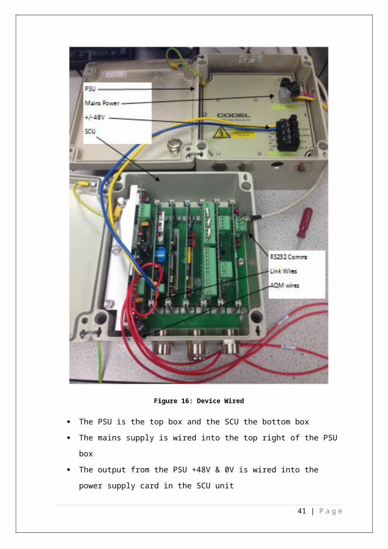
The device was wired as laid out in the introduction with no complications.

Figure 16: Device Wired

The PSU is the top box and the SCU the bottom box

The mains supply is wired into the top right of the PSU box

The output from the PSU +48V & 0V is wired into the power supply card in the

SCU unit

31 | P a g e

The link wires between the PSU unit and the AQM are the two small red wires in

the bottom left hand side of the SCU box

The four long red wires went to the AQM (see below)

Figure 17: AQM Wired

The top right hand side of the SCU box is the RS232 communications port which

feeds into the system running Codel’s software

32 | P a g e

2.1.1Wiring the RS232 Communications

The RS232 connection had to be soldered together, the following schematic was used:

Figure 18: RS232 Female Pin out [13]

The connection was soldered together using the above pin out.

Figure 19: RS232 Soldered Connection

33 | P a g e

2.2 Software Configuration

2.2.1 Alignment

The device must be aligned before use, the sensor and reflector must be carefully aligned

for the full capabilities of the sensor. However, for the purpose of this project the sensor

was not mounted on a wall which it is designed for. The device was operated while being

situated on a window sill in the air quality lab above the college car park. This location was

chosen to monitor the pollutant concentrations from the car park traffic. For the device to

work to work to its full capabilities it should be perfectly aligned which would require

proper mounting and installation of the device.

To align the device the AQM should be fixed and the reflector should be tweaked as it is

more sensitive to movement of the two. For optimum performance the desired readings are

CO = 90 and VIS = 60. An error of ±5 is accepted for data recording.

Figure 20: Detector Aligned

Black background on the alignment screen indicates the data is okay, if the background is

red (figure 21) it indicates the device is saturated.

34 | P a g e

Figure 21: Saturated Detector

The background can flash blue also; this means there is a communication error. It is

common for the occasional blue flash during transmission. When the sensors are

completely out of line we get a reading of 0 for Vis and 255 for CO & NO.

Figure 22: Detector Misalignment

35 | P a g e

2.2.2 Detector Levels

The detector levels indicate the typical ranges for the measurements parameters. The

following image indicates the typical ranges for correct performance:

Figure 23: Detector Levels Range [1]

The measurement process will indicate a detector saturation condition by switching the

saturation indicator from green to red if the signal strength of the detector is too high. The

gain should be reduced if the red indicator is observed.

Figure 24: Detector Level Saturated

Vis Rx is saturated; this can happen if the path length is too short. (3m is recommended)

36 | P a g e

2.2.3 Thermistor Control

The lead selenide detector, used for CO & NO measurements, incorporates a thermistor for

sensing and a Peltier-cooled element for control of the detector temperature. Changing the

thermistor control parameters from the factory settings will result in unstable

measurements. The thermistor control should be on auto control and have a cooler current

of approximately 800 mA.

Figure 25: Thermistor Control

The cooler current in the image above is 6064 (x10) = 606 mA.

37 | P a g e

2.2.4 Output

The output mode displays output value data for CO, NO and visibility channels. The

standard output screen is below and this indicates the device is in calibration mode. (See

calibration 2.2.6)

Figure 26: Output Configuration

The opacity reading describes the transparency level, where 1 is not transparent and

0 is fully transparent. Opacity will increase as CO & NO levels increase.

Vis metres will decrease as our CO & NO levels increase, this is expected as the

more gas present in the path length the less visibility

38 | P a g e

2.2.4.1 Instantaneous v Smoothed measurement

The software allows data to be measured in two forms, instantaneous and smoothed. An

instantaneous measurement is the data measured at that particular instant. Smoothed

measurements are the data measured averaged over a time period.

2.2.5 Y-Values

These values are used by the processor to compute concentration levels for CO & NO in

ppm. The standard output screen is below and this indicates the device is under zero gas

conditions.

Figure 27: Y-Values

The Y value can be calculated and checked using the calibration data.

39 | P a g e

1. Y (CO) = 90,000 – (Set Cal CO) * CO Measured / CO Reference

90,000 – (55,118) * (13,608 / 9,397)

= 10,182 Actual value for Y (CO) = 10,241

2. Y (NO) = 90,000 – (Set Cal NO) * NO Measured / NO Reference

90,000 – (57,092) * (10,045 / 7,149)

= 9781 Actual value of Y (NO) = 9,818

2.2.6 Calibration

Like any measurement system Codel’s AQM must be calibrated regularly to maintain

highly accurate and reliable data. To calibrate select ‘ON’ and click ‘APPLY’. Please note,

after a power-up and after an interruption of the optical beam for more than 10 seconds, the

instrument automatically switches to calibration mode for 240 minutes and 30 minutes

respectively. The automatic calibrations can be stopped by selecting ‘Send’ screen and

sending the file ‘calstop.dtx’ to the AQM master processor.

Figure 28: Stop Calibration

40 | P a g e

After the file is sent it takes approximately 10 seconds and a relay trip can be heard in the

station control unit box. Then select calibrate ‘OFF’ and the device will be forced out of

calibration mode.

2.3 Testing

2.3.1 Overnight data recording

The device was left recording data from 6pm-12am the next day; it recorded small levels

of CO ranging from 0-5 ppm. This is expected as the device location is 20 m from the

small car park.

The following images are CO and visibility levels at 11am.

Figure 29: CO Overnight Recording

There is a correlation between CO levels rising (0 to 5 ppm) and Visibility levels falling

(9999 to ~825).

Figure 30: Visibility Overnight Recording

41 | P a g e

2.3.2 Bump Test

The idea of the bump test (also known as spike test) is to introduce high levels of gases

into the device and the data measurements should record the spike in readings. It proves

the system is recording data and also checks the range of the instrument. To do a bump test

the system had to be sealed to allow the sensor record the data rather than it escaping into

the atmosphere .The gas sample was acquired from the exhaust from a petrol engine car.

The system was crude and simple but sufficient for the purpose of this experiment. A

plastic pipe was used to connect the sensor to the reflector with the ends sealed with soft

tissue. The gas bag had an extraction pipe and a valve to control the flow and this was fed

into the inlet valve located on the centre of the pipe.

Figure 31: Experimental Set-Up

42 | P a g e

CO levels went from 0 – 1376 ppm before the device was over saturated and cut

into calibration mode

No levels went from 0 – 10 ppm

Opacity went from 0 – 60 and slowly decreased back down as gas escaped to 0

(fully transparent air)

Vis metres went from 9999 – 1872 as the gas entered the system and the clear

transparent air got replaced with polluted fumes.

Note: Further analysis of the bump test is done in the results section 3.2.1 and 3.2.2

2.3.3 Cross Calibration Test

The next experiment undertaken was a cross calibration of Codel’s AQM and Alpha Sense

CO sensor. CO levels were compared between the two. The experimental setup for this

was similar to bump test with the addition of an outlet pipe leading the gas into the alpha

sense probe before it exited the system. The red lines show the gas flow.

Figure 32: Cross-Calibration Test

The alpha sense probe is on the left hand side of the above picture in a sealed plastic

container.

Note: Detailed analysis of the cross calibration test is done in the results section.

43 | P a g e

2.3.4 Technical Specs for Carbon Monoxide Alpha Sense Probe

Measuring units are ppm

Measurement range of 0-1000 ppm, this is the range for which the error obtained

does not exceed the maximum permissible error

Temperature range of -30°C to 50°C

Sensitivity in 400 ppm CO is 55 to 90, this is ability to respond to small physical

differences

Response time from 0 – 400 ppm CO is < 25, this is the time taken by the sensor to

approach its true output after being subject to corresponding input

Zero Drift ppm equivalent change/year in a lab of < 0.2

Resolution ppm equivalent < 0.5, this is the smallest change a sensor can detect in

the quantity that it is measuring

44 | P a g e

Chapter 3

Analysis of Results

3.1 Ambient Monitoring

The test involved the Codel sensor monitoring ambient air from 12 pm to 1 am the

following day, the maximum CO reading per half hour was plotted against the time of day.

45 | P a g e

12:00:00 PM

01:40:48 PM

03:21:36 PM

05:02:24 PM

06:43:12 PM

08:24:00 PM

10:04:48 PM

11:45:36 PM

01:26:24 AM0

0.5

1

1.5

2

2.5

3

3.5

Ambient Monitoring (CO)

Time of Day

CO (p

pm)

Figure 33: Ambient Monitoring (CO)

The data monitoring proved inconclusive with the max CO reading recorded being 3 ppm.

With the accuracy of the sensor being +/- 1 ppm these small readings could be contributed

to noise. The location of the sensor was 20m from the car park and with no air being

pumped into the lab where the device is located on the window sill; the low readings

recorded are no surprise.

3.2 Bump Tests

3.2.1 Bump Test 1

The test was undertaken for Codel’s AQM with safety measures in place as carbon

monoxide is highly dangerous in high concentrations. Carbon monoxide was forced from

the gas bag into the sealed system via the inlet tube (See figure 31).

46 | P a g e

0 50 100 150 200 2500

200

400

600

800

1000

1200

AQM Bump Test 1 (CO)

Time (s)

CO (ppm)

Figure 34: Bump Test 1 (CO)

The device read CO levels from 0 ppm up to 1376ppm before the device was over

saturated and the instrument cut into calibration. The sensor went into calibration outside

the specified operating range (1376 ppm > 1000 ppm) which is expected. Nitric Oxide

(NO) also spiked slowly from 0-10 ppm but the main pollutant present from exhaust

emissions was the carbon monoxide.

47 | P a g e

0 50 100 150 200 250 300 350 400 450 5000

2

4

6

8

10

12

AQM Bump Test 1 (NO)

Time (s)

NO

(ppm

)

Figure 35: Bump Test 1 (NO)

3.2.2 Bump Test 2

The test was repeated the following day after the system was flushed out and re-aligned

and calibrated.

0 50 100 150 200 2500

200

400

600

800

1000

1200

AQM Bump Test 2 (CO)

Time (s)

CO (ppm)

Figure 36: Bump Test 2

The results were similar with the sensor reading CO levels from 0 ppm up to 1464 ppm

before the device was over saturated and cut into calibration mode.

48 | P a g e

Codel’s software also graphs the data; the y axis needs a multiplier of X100. A section of

the graph can be magnified by clicking and dragging the cursor across the required area.

Figure 37: Codel's Graph Plot

Codel’s air quality monitor has a measurement range of 0 – 1000 ppm. Above 1000 ppm

the sensor becomes over saturated and the device cuts into calibration. (1464 ppm here)

While the gas enters the sealed system the air molecules become flushed with gas

molecules leaving the visibility in the system to decrease. This is an important parameter

when the device is installed in a busy tunnel. The following image is the visibility curve as

gas was forced from gas bag into the system. The Y axis has a multiplier of x100 with

units of metres.

49 | P a g e

Figure 38: Visibility Graph

Vis metres went from 9999 – 1872 as the gas entered the system and the clear

transparent air got replaced with polluted fumes.

The troughs are subject to the force being placed on the gas bag and the influx of gas

molecules decreasing the visibility of air, while the system is sealed for the gas to remain

in the pipe long enough for the sensor to read the gas levels, the gas will escape at the pipe

ends causing the crest effect.

50 | P a g e

3.3 Cross Calibration Test

The comparison test was done with alpha sense probe which range is also 0 -1000 ppm.

The gas was fed from the air quality monitor to the alpha probe with both instruments

recording CO levels.

0 50 100 150 200 250 300 350 400 450 5000

200

400

600

800

1000

1200

Codel & Wolfesense Comparison

CodelWolfesense

Time (s)

C0 (p

pm)

Figure 39: Cross Calibration Test

We can see the correlation of data with both instruments recording similar CO levels. The

difference in the data is due to the system design; the data shows gas escapes from the

system before reaching the Alpha Sense probe. However, the correlation of the probes

shows the instruments recording accurate concentrations of carbon monoxide.

51 | P a g e

3.4 Report Generation

The software also allows the user to generate a report at any time and records all readings

at that time (Y values, thermistor, detector levels, output, and calibration).

Figure 40: Report Generation

The serial number of the air quality monitor used is stated 0298

In this report the output of CO is 1317 ppm

The high concentrations recorded cause the CO detector levels (range 15000-

25000) to crash down to ~4500

52 | P a g e

Chapter 4

Concluding Remarks

53 | P a g e

4.1 Discussion

The air quality monitor was wired from the schematics provided in the instrument manual.

The station control unit (SCU) was connected for communications and the power supply

unit (PSU) to the mains supply. A RS232 connection was used to transfer data from the

SCU to the PC running Codel’s software. The main issue for testing and calibration of the

instrument was the alignment. The device is designed for horizontal mounting on a wall.

The project was done with the device resting on window sill and alignment of the device

was extremely tough and time consuming, small movements as little as one millimetre can

cause miss-alignment. Post-test the device can be saturated and needs a settling time along

with re-calibration which can take up to four hours; this made the testing phase difficult.

CO & NO measurements were taken for installation purposes for Cork Institute of

Technology with possible sites being the mechanics workshop were combustion engines

are used indoors and the work yard were deliveries take place. Co levels up to 15 ppm

were recorded and with a resolution of 1 ppm for codel’s sensor this would be a viable

option for installation.

4.2 Future Work

Recommended installation and mounting of the device would improve the sensor’s

alignment and increase the accuracy of measurements recorded and allow the device to be

used to its full capabilities. Another recommendation is to install network infrastructure to

allow remote access to the device.

4.3 Conclusion

The air quality monitor was re-commissioned back to working order with all wiring done

as per schematics in the manual. Codel’s WinCom software was installed to run the device;

it is connected via the RS232 connection in the station control unit. The sensor and

reflector were carefully aligned with the path length being the recommended 3 m (6 m

folded beam).Pre alignment the senor had to be calibrated; the software includes an inbuilt

calibration function which takes up to 4 hours after a power up. The device was left

monitoring ambient air from the nearby car park but the test proved inconclusive as the

maximum CO value recorded was 3 ppm. With the accuracy of the sensor being +/- 1 ppm

54 | P a g e

the small levels detected could be down to noise. With no air being pumped into the lab

were the device was located it was going to be a struggle to pick up plausible readings. The

working status of the device was checked via a bump test using gaseous fumes from a car

exhaust. The sensor’s range is 0-1000 ppm for CO and the bump test showed the device

being saturated and cutting out at 1376 ppm CO. Nitric oxide levels were not heavily

present as the NO output went from 0 – 10 ppm. The increase in pollution caused an

expected consequential decrease in visibility. Visibility dropped from full visibility reading

of 9999 to low visibility of 1872. This effected the opacity reading which went from 0

(fully transparent air) to 60 (semi-transparent air). The sensor operated under as expected

under the extreme influx of pollutants. The sensor was compared with another leading

manufacturer of CO probes called Alpha Sense, the system design was modified (See

figure 32) with the gas entering codel’s path length before travelling to the alpha probe, the

correlation of data showed similar CO values with alpha probe recording slightly less CO

concentrations which is expected due to some gas escaping in the system at each end of the

plastic pipe. This validated the integrity of the measurements by Codel’s air quality

monitor by comparing it with the measurements recorded by the standard lab device sensor

(Alpha Sense). The device was re-commissioned back to working order, calibrated by the

WinCom software and validated by the cross calibration test with the laboratory probe

(Alpha Sense). Overall the project was a success and the required tasks were

accomplished.

55 | P a g e

References

1. http://en.wikipedia.org/wiki/Carbon_monoxide_poisoning

2. Codel Tunnel Craft 3 technical manual

3. http://www.detcon.com/electrochemical01.htm

4. FPO. (2004). Electrochemical gas detector and method of using same. Available:

http://www.freepatentsonline.com/4141800.html. Last accessed 20 Feb 2015.

5. Muda, R. (2009). Simulation and measurement of carbon dioxide exhaust

emissions using an optical-fibre-based mid-infrared point sensor. Journal of Optics

A: Pure and Applied Optics, 11(1)

6. Figaro Sensor. (2003). General Information for TGS Sensors. Retrieved February

28, 2010, from http://www.figarosensor.com/products/general.pdf

7. Naranjo, E. (2007). Ultrasonic Gas Leak Detectors. Retrieved February 27, 2010,

from http://www.gmigasandflame.com/article_october2007.html

8. Codel. (2011). Tunnel Atmosphere Monitoring. Available:

http://www.forbesmarshall.com/fm_micro/downloads/Codel/AQM.pdf. Last

accessed 20 Feb 2015.

9. Sense Air. (2000). Measuring method for emissions in road tunnel

systems. Available: http://senseair.se/wp-content/uploads/2011/05/14.pdf. Last

accessed 24th Feb 2015.

10. Csep. (2015). Atomic absorption and emission spectra. Available:

http://csep10.phys.utk.edu/astr162/lect/light/absorption.html. Last accessed 3rd

May 2015.

11. SenseAir. (2010). Gas Application. Available:

http://www.senseair.se/senseair/gases-applications/carbon-monoxide/. Last

accessed 3rd May 2015.

12. 11.Electro-Optics. (2010). Silicon Photo detectors. Available:

http://www.eotech.com/cart/category4/photodetectors/silicon-photodetectors. Last

accessed 20 Feb 2015.

13. 12.Servomex. (2009). Gas filter correlation. Available:

http://ww3.servomex.com/gas- analyzers/technologies/gas-filter-correlation. Last

accessed 20 Feb 2015.

14. http://pixshark.com/rs232-female-pinout.htm

56 | P a g e