film formation of water-borne polymer dispersion: … · film formation of water-borne polymer...
TRANSCRIPT

Film Formation of Water-borne Polymer Dispersion: Designed Polymer Diffusion for High Performance
Low VOC Emission Coatings
by
« Mohsen Soleimani Kheibari »
A thesis submitted in conformity with the requirements for the degree of Doctor of Philosophy
Graduate Department of Chemical Engineering and Applied Chemistry University of Toronto
© Copyright by Mohsen Soleimani Kheibari 2012

ii
Film Formation of Water-borne Polymer Dispersion: Designed
Polymer Diffusion for High Performance Low VOC Emission
Coatings
Mohsen Soleimani
Doctor of Philosophy
Department of Chemical Engineering
University of Toronto
2012
Abstract
In this thesis, I describe experiments that were designed to provide a better
understanding of polymer diffusion during latex film formation. This step leads to the
improvement of film mechanical properties. Polymer diffusion in these films was
monitored by fluorescence resonance energy transfer. Current paint formulations contain
Volatile Organic Compounds (VOCs) as plasticizers to facilitate polymer diffusion. The
drawback of this technology is the release of VOCs to the atmosphere. VOCs are
deleterious to the environment and contribute to smog and ground level ozone formation.
The propensity of water, an indispensible part of any latex dispersion, to promote
polymer diffusion was studied. Copolymers of poly (butyl acrylate-co-methyl
methacrylate) and poly(ethylhexyl acrylate-co-tertiary butyl methacrylate) with similar

iii
glass transition temperatures but different hydrophobicity were compared. Polymer
diffusion was monitored for films aged at different relative humidities. Water absorbed
by the hydrophobic copolymer film was less efficient in promoting polymer diffusion
than in the hydrophilic polymer. Only the fraction of water which is molecularly
dissolved in the film participate actively in plasticization. Although water has low
solubility in most latex polymers, molecularly dissolved water is more efficient than
many traditional plasticizers.
The possibility of modifying film formation behavior of acrylic dispersions with
oligomers was studied by synthesizing hybrid polymer particles consisting of a high
molecular weigh (high-M) polymer and an oligomer with the same composition.
Oligomers with lower molecular weight are more efficient as diffusion promoters and
have less deleterious effect on high-M polymer viscosity.
A different set of hybrid particles were prepared in which the oligomer contained
methacrylic acid units. The composition of the oligomer was tuned to be miscible with
the high-M polymer when the acid groups were protonated but to phase separate when
the acid groups were deprotonated. At basic pH, these particles adopt a core-shell
morphology, with a shell rich in neutralized oligomers. After film formation, the
oligomer shell retarded polymer diffusion. This retardation is expected to expand the time
window during which the paint surface can be altered without leaving brush marks (open
time). Short open time is a pressing problem in current technology.

Acknowledgement
I would like to express my deepest gratitude to my supervisor, Professor Mitchell A.
Winnik for his supervision and guidance during my graduate studies at University of
Toronto. His deep insight, continuous encouragements and approachable attitude always
provide a strong support for my research. I found Mitch extremely resourceful not only
about research related problems but also about any other problem I needed advice on. I
enjoyed his generosity in allowing me to pursue my own ideas and research directions. I
am all honored to have him as my advisor.
I would like to use this opportunity to thank Dr. Willie Lau from Rohm and Hass (now
Dow Advanced Materials). Interacting with Willie during my research was indeed an
invaluable opportunity. He made his supports available in several ways. Many ideas in
this thesis were developed during discussions with him. During these discussions, I came
to appreciate the importance of industrial research and developed a practical way of
thinking about scientific problems.
My appreciation will go to my research committee, Professor Eugenia Kumacheva,
Professor Tim Bender and Professor Yu Ling Cheng for their advices and suggestions.
Thanks are due to Dr. David Mendenhall for synthesizing a benzophenone derivative in a
large scale. I also would like to thank Rohm and Hass, NSERC Canada for their support
of this research, and the Province of Ontario for an OGS fellowship.
My time during graduate studies was enriched by interactions and discussions with
fellow colleagues and friends. I am particularly grateful to Dr. Jeff Haley, Dr. Gerald
Guerin, Dr.Yuanqin Liu, Dr. Neda Felorzabihi, Dr. Conrad Seigers, Dr. Stuart Thickett,
Dr. Daniel Majonis and Dr. Sheng Dai. I would like to thank all the current and former
members of Mitch research group.
My father, Mr. Mohammad Soleimani, was my first chemistry teacher and it was under
his mentorship that I began my journey in chemistry. During these years I have always
enjoyed an unyielding support of my family. I could not have accomplished this research
without their constant love and affection. I dedicate this thesis to them for their endless
love.
iv

Table of Contents
CHAPTER ONE
Introduction................................................................................................................................... 1
1.1 Scope and objectives of this research .............................................................................. 1
1.2 Latex film formation and polymer diffusion ................................................................... 2
1.3 Thesis outline ................................................................................................................... 4
1.4 References........................................................................................................................ 6
CHAPTER TWO
Fluorescence Resonance Energy Transfer (FRET) Principles and Its Application in
Film Formation Study .................................................................................................................. 7
2.1 Basic principles................................................................................................................ 7
2.2 Fluorescence resonance energy transfer for a single donor-acceptor pair ....................... 9
2.3 FRET in homogeneous systems..................................................................................... 12
2.4 FRET application in film formation processes .............................................................. 13
2.5 Fluorescence intensity decay measurements ................................................................. 14
2.6 Calculation of energy transfer quantum efficiency........................................................ 16
2.6.1 Fitting experimental data ................................................................................... 18
2.6.2 Polymer diffusion coefficient ............................................................................ 21
2.7 Monte Carlo calculations of energy transfer.................................................................. 24
v
2.8 Interface thickness measurements using FRET ............................................................. 30
2.9 Summary ........................................................................................................................ 33
2.10 References.................................................................................................................... 34
CHAPTER THREE
Effect of Hydroplasticization on Polymer Diffusion in Poly (butyl acrylate-co-methyl
methacrylate) and Poly (2-ethylhexyl acrylate -co- tert-butyl methacrylate) Latex
Films............................................................................................................................................. 36
3.1 Introduction.................................................................................................................... 36
3.2 Experimental .................................................................................................................. 39
3.2.1 Materials ............................................................................................................ 39
3.2.2 Latex preparation and characterization.............................................................. 39
3.2.3 Rheology measurements .................................................................................... 42
3.2.4 FTIR measurements ........................................................................................... 42
3.2.5 FRET measurements.......................................................................................... 43
3.3 Results and Discussion .................................................................................................. 44
3.3.1 Preparation and characterization of latex samples............................................. 44
3.3.2 Energy transfer studies of polymer diffusion..................................................... 45
3.3.3 Polymer diffusion at different temperatures. ..................................................... 47
3.3.4 Effect of humidity on polymer diffusion: hydroplasticization .......................... 53
3.3.5 FTIR analysis of water content in the films....................................................... 60
3.4 Summary ........................................................................................................................ 65
vi

3.5 References............................................................................................................. 67
Appendix 1
Transmission FTIR spectra for films of P(BA MMA ) and P(EHA tBMA ) aged at
different relative humidities
50 49 50 49
.......................................................................................................... 71
CHAPTER FOUR
Effect of molecular weight distribution on polymer diffusion rate during film
formation of hybrid two-component high/low-molecular weight latex particles.................. 72
4.1 Introduction.................................................................................................................... 72
4.2 Experimental .................................................................................................................. 77
4.2.1 Materials ............................................................................................................ 77
4.2.2 Synthesis of Dimethylamino-2-methacryloxy-5-methylbenzophenone.
(NBen-MA)................................................................................................................. 77
4.2.3 Synthesis of dispersions..................................................................................... 78
4.2.4 Modifying high molecular weight particles with oligomer ............................... 79
4.2.5 Characterization of the dispersions.................................................................... 80
4.2.6 Stage ratio measurement .................................................................................... 81
4.2.7 Film formation and FRET measurments............................................................ 81
4.2.8 Rheology measurements .................................................................................... 83
4.3 Data and Data Analysis.................................................................................................. 83
4.4 Results and Discussion .................................................................................................. 86
4.4.1 Latex dispersion synthesis ................................................................................. 86
vii

4.4.2 Oligomer content measurements........................................................................ 90
4.4.3 Effect of oligomer on the diffusion rate of high molecular weight
polymers...................................................................................................................... 92
4.4.4 Effect of oligomer molecular weight on diffusion rate...................................... 94
4.4.5 Latex blending experiments............................................................................... 99
4.4.6 Effect of oligomer on polymer rheological properties..................................... 101
4.5 Summary ...................................................................................................................... 104
4.6 References.................................................................................................................... 106
CHAPTER FIVE
Synthesis of Smart Polymer Nanoparticles and Their Application as
Environmentally Compliant Coatings .................................................................................... 109
5.1 Introduction.................................................................................................................. 109
5.2 Experimental ................................................................................................................ 110
5.2.1 Materials .......................................................................................................... 110
5.2.2 Nanoparticle synthesis ..................................................................................... 112
5.2.2.1 First stage seeded emulsion polymerization ........................................ 112
5.2.2.2 Second stage seeded emulsion polymerization.................................... 112
5.2.3 Instrumentation and analysis............................................................................ 114
5.2.3.1 Fluorescence decay measurements ...................................................... 114
5.2.3.2 Dynamic Light Scattering (DLS)......................................................... 114
5.2.3.3 Dispersion dialysis ............................................................................... 114
viii

ix
5.2.3.4 Differential Scanning Calorimetry (DSC) ........................................... 114
5.2.3.5 Gel Permeation Chromatography (GPC) ............................................. 115
5.2.3.6 Nuclear Magnetic Resonance (NMR) measurements.......................... 115
5.2.3.7 Capillary Hydrodynamic Fractionation (CHDF) ................................. 116
5.2.3.8 Acid-base titrations .............................................................................. 116
5.2.3.9 Equilibrium water content measurements............................................ 117
5.3 Results and Discussion ................................................................................................ 117
5.3.1 Morphology transformation caused by a change in pH................................... 125
5.3.2 Promotion of polymer diffusion by the acid-rich oligomer ............................. 133
5.3.3 Retarded coalescence: the early stage of film formation at acidic and
basic pH .................................................................................................................... 137
5.4 Summary ...................................................................................................................... 142
5.5 References.................................................................................................................... 144
Appendix 2
pH response of particles loaded with styrene-free oligomers............................................ 146
Appendix 3
Chemical structure of TexanolTM....................................................................................... 150

Declaration
No part of this thesis has been previously published in any journal by any person except
where due reference has been made in the text. To the best of the author’s knowledge,
this thesis contains no material previously written towards any degree in any university.
x

List of Tables
Table 2.1. Notations used for referring to different types of fluorescence decay profile.............................................................................................................15
Table 3.1. Recipes for the synthesis of labeled and non-labeled latex dispersions.........40
Table 3.2. Characterization of latexes used in this study. ...............................................46
Table 3.3. The initial and final energy transfer efficiency ΦET(0)..................................47
Table 3.4. Vertical shift factors and equilibrium water content at different humidities.......................................................................................................55
Table 3.5. Spectroscopic parameters of water absorbed to P(BA50MMA49) at different water activities in the film (relative humidity). .............................................61
Table 3.6. Spectroscopic parameters of water absorbed to P(EHA50tBMA49) at different water activities in the film (relative humidity). At aw=0.23 the analysis was not possible due to very low water content....................................................63
Table 4.1. Recipes for the synthesis of labeled and non-labeled latex dispersions.........78
Table 4.2. Typical second-stage seeded emulsion polymerization recipe for the synthesis of hybrid particles containing various amount of oligomer synthesized with 7 wt% C12-SH. ..................................................................................................80
Table 4.3. Characterization of dispersions and dispersion polymers. .............................87
Table 4.4. Characteristics of the acceptor-containing particles used in FRET studies. ...........................................................................................................89
Table 4.5. Vertical shift factors (aO) obtained from master curve analysis for samples containing different amounts of oligomers with various Mn. ........................96
Table 4.6. The Cross model parameters for flow curves obtained at a common (Texp-Tg) as shown in Figure 4.13. ................................................................................103
Table 5.1. Synthesis of the dye-labeled composite particles...........................................113
Table 5.2. Characterization of the nanoparticle dispersions used in this study. .............123
xi
List of Figures
Figure 1.1) Mechanism of film formation from aqueous polymer dispersion (latex). ...2
Figure 1.2) A) chemical structure of polymerizable fluorophores used in this study. B) A mixture of donor- and acceptor-labeled particles. Water and hydrophilic materials at the interface prevent diffusion. Mixing process occurs only after intimate contact between labeled polymers. ..................................................3
Figure 2.1) Jablonski diagram for fluorescence resonance energy transfer (FRET). ....9
Figure 2.2) Schematic representation of angles involved in measurement of κ2 (eq 2.9). ..........................................................................................................10
Figure 2.3) A) An example of fitting fluorescence decay profile to eq 2.22 using Levenberg-Marquardt algorithm. The weighted residuals (B) and the autocorrelation function (C) appears randomly distributed around zero. The χ2 was 1.06 for this fit. .......................................................................................21
Figure 2.4) Schematic representation of the core-shell geometry used for Monte Carlo calculations of energy transfer efficiency. .....................................................25
Figure 2.5) Normalized concentration profiles predicted by the Fickian diffusion model in a coreshell geometry (Rp = 67 nm and a = 143.6 nm) for x=5 nm (A) and x=500 nm (B). Dashed lines represent CD (donor concentration) and solid lines represent CA=1-CD (acceptor concentration). C) Simulated donor decay profile corresponding to the concentration profiles shown in (A) and (B)....26
Figure 2.6) Evolution of the energy transfer efficiency (ΦET) calculated from simulated decays in a core shell geometry (Rp = 67 nm and a = 143.6 nm) as Fickian diffusion proceeds (increasing extent of diffusion, x). ..................................28
Figure 2.7) Plots of the extent of diffusion vs square root of time at four annealing temperatures. The lines are best-fitted lines to the data points. The linear relation between x and t1/2 points to a Fickian diffusion mechanism.............29
Figure 2.8) Polymer segment density profiles across the interface between a two immiscible polymers. The definition of the interface thickness (δ) is shown.. ...........................................................................................................30
Figure 2.9) A) radial distribution function of acceptor-labeled polymer for core-shell particles with Rs = 55 nm and Rp = 78 nm with three different interface thickness (δ). B) Simulated donor decay profile corresponding to the concentration profiles shown in (A). .............................................................32
Figure 2.10) Values of energy transfer efficiency (ΦET) calculated from simulated decays in a core-shell geometry (Rs = 55 nm and Rp = 78 nm) for various interface thicknesses (δ)................................................................................................33
xii

Figure 3.1) Plots of the energy transfer efficiency ΦET vs. time for A) P(BA50MMA49) and B) P(EHA50tBMA49) at 40, 50, 60 and 70 °C. .......................................48
Figure 3.2) Plots of the fraction of mixing fm vs. time for A) P(BA50MMA49) and B) P(EHA50tBMA49) at 40, 50, 60 and 70 °C. ...................................................49
Figure 3.3) Plots of the apparent diffusion coefficient Dapp vs. fraction of mixing fm for A) P(BA50MMA49) and B) P(EHA50tBMA49) at 40, 50, 60 and 70 °C, The master curves are shifted one unit down for clarity. For P(BA50MMA49) , Ea = 38.5 kcal/mol and for P(EHA50tBMA49), Ea = 35.7 kcal/mol were used as shift factors.....................................................................................................50
Figure 3.4) ln(Dapp) vs. 1000/T for P(BA50MMA49) at two different fractions of mixing. The slope of the line corresponds to the activation energy............................51
Figure 3.5) Plots of the master curves of the shear storage (G’) and loss (G’’) moduli for A) P(BA50MMA49) and B) P(EHA50tBMA49). ............................................52
Figure 3.6) Plots of the ln(aT) against the inverse of the absolute temperatures for A) P(BA50MMA49) and B) P(EHA50tBMA49)...................................................53
Figure 3.7) Plots of the energy transfer efficiency ΦET vs. time for A) P(BA50MMA49) and B) P(EHA50tBMA49) at 0, 23, 54, 85 and 98% RH and 25 °C...............54
Figure 3.8) Plots of the apparent diffusion coefficient Dapp vs. aging time for A) P(BA50MMA49) and B) P(EHA50tBMA49) at 0, 23, 54, 85 and 98% RH and 25 °C, The master curves are shifted one unit down for clarity. ...................56
Figure 3.9) Plots of 1/ln(aH) vs. φw-1 based on the data in Table 3.4 For
P(EHA50tBMA49) the intercept and slope of the line are 0.530 and 0.004 respectively (R2 = 0.97). For P(BA50MMA49) the intercept and slope of the line are 0.205 and 0.004 respectively (R2 = 0.99)..........................................58
Figure 3.10) Plots of 1/ln(aH) vs. φw-1 where the intercept was fixed to the polymer free
volume at 25° C. For P(EHA50tBMA49) the slope of the line is 0.0055 (R2 = 0.77). For P(BA50MMA49) the slope of the line is 0.0045 (R2 = 0.95). ........59
Figure 3.11) FTIR spectra (in the OH stretching region) of water absorbed into the copolymer films at different relative humidities............................................60
Figure 3.12) Curve-fitting analysis results of isolated FTIR spectra obtained on films aged at 98% RH. A) P(BA50MMA49) and B). P(EHA50tBMA49). ...............62
Figure 3.13) Schematic representation of polymer films aged at different humidities. A) Films aged at lower humidities contained only molecularly dispersed water. B) At higher humidities, water absorbed in the film phase separates to form water pools. At 98% RH, these water pools were large enough to scatter light and the films appeared turbid to the naked eye..............................................64
xiii
Figure 3.14) Reconstructed Fujita plots based on the dual nature of water. The dashed area represents the phase-separated water in the films. .................................64
Figure A1.1) Transmission FTIR spectra for films of A) P(BA50MMA49) and B) P(EHA50tBMA49) aged at different relative humidities. ...............................71
Scheme 4.1) Synthesis strategy used for the preparation of two-component nanoparticles containing acceptor-labeled P(BA50MMA49) and a fraction of a non-labeled oligomer...............................................................................................................76 Figure 4.1) The UV calibration curve for A-P(BA50MMA49) in THF. This curve was
used to calculate the amount of labeled polymer in THF solutions of hybrid particles. .........................................................................................................82
Figure 4.2) ΦET values calculated by analyzing ID(t) decay profiles using the model-free approach() and the Monte Carlo approach () for P(BA50MMA49)4_37%. ....................................................................................84
Figure 4.3) A) Chromatograms of samples synthesized with different amounts of C12-SH in the recipe and B) plot of 1/Mn and PDI against [C12-SH] for P(BA50MMA49) dispersions. C) Chromatograms of samples withdrawn during a synthesis with 4 wt% of C12-SH at different feed time. D) The evolution of number average molecular weight (Mn) and PDI for samples shown in (C)...................................................................................................88
Figure 4.4) Glass transition temperatures of samples described in Table 4.4 as a function of their oligomer content (Woligomer). Solids lines represents the Fox-Flory prediction based on the Tg value of A-P(BA50MMA49) and the Tg values of the individual oligomers (Table 4.3)..............................................................91
Figure 4.5) FRET results for samples prepared by in situ generation of oligomer with 11% C12-SH added to the second reaction recipe. A) Fraction of mixing fm as a function of aging time for samples containing different amounts of the oligomer. B) Apparent diffusion coefficient Dapp as a function of fm for samples containing different amounts of the oligomer. The lowermost curve labeled “M” is the master curve prepared by shifting the data toward 0% curve. The master curve was moved one unit down for clarity. All lines are guides for the eye. ..........................................................................................93
Figure 4.6) Plots of the mixing fraction vs annealing time for samples to which different amounts of oligomers with A) Mn = 3k and B) Mn = 4.9k were incorporated in situ..................................................................................................................94
Figure 4.7) Apparent diffusion coefficient Dapp as a function of fm for samples containing different amounts of oligomer synthesized with A) 7 wt% C12-SH in the second stage recipe and B) 11 wt% C12-SH in the second stage recipe. The lowermost curve in each plot, labeled “M”, is the master curve prepared by shifting the data toward 0% curve. The master curve was moved one unit down for clarity. All lines are guides for the eye...........................................95
xiv

Figure 4.8) Plots of the master curves of G’ and G’’ for A-P(BA50MMA49), latex
polymer at a reference temperature T0 =70 °C..............................................97
Figure 4.9) Plot of the Ln (aT) against the inverse of the absolute temperature for A-P(BA50MMA49). WLF parameters were obtained from the fit to the experimental data. ..........................................................................................97
Figure 4.10) Plots of 1/Ln(aO) vs φO-1 based on the data presented in Table 4.5 for in situ
incorporation of oligomers with A) Mn=2.0k, the slope of the line is 0.066 (R2=0.96); B) Mn=3.0k, the slope of the line is 0.114 (R2=0.99); C) Mn=4.9k, the slope of the line is 0.132 (R2=0.96)..........................................................98
Figure 4.11) FRET results for blending experiments: plots of the mixing fractions for samples in which P(BA50MMA49) was blended with different amounts of oligomers with A) Mn = 2k, B) Mn = 3k and C) Mn = 4.9k. Plots of the apparent diffusion coefficient vs mixing fraction (D, E and F) when oligomers with 2, 3 and 4.9k Mn were used, respectively. Curves labeled with ‘M’ are master curves built by vertical shifting as described in the main text. All master curves were shifted one unit down for clarity. All lines are guides for the eye. ...........................................................................................................100
Figure 4.12) Plots of 1/Ln(aO) vs φO-1 for films prepared by blending oligomers of
different Mn A) Mn=2.0k, the slope of the line is 0.057 (R2=0.98); B) Mn=3.0k, the slope of the line is 0.078 (R2=0.98); C) Mn=4.9k, the slope of the line is 0.087 (R2=0.96). ............................................................................101
Figure 4.13) Plots of shear viscosity (η) as a function of shear rate for A-P(BA50MMA49) at 113 °C; and for the two-component samples to which 20 wt% of the 2.0k oligomer; 30 wt% of the 3.0k oligomer and 40 wt% of the 4.9k oligomer was incorporated. The measurements on the two-component samples were performed at 100 °C. The lines represent best-fit curve according to the Cross model..............................................................................................................102
Figure 5.1. Film formation by soft polymer nanoparticles covered with an oligomeric shell a) before the end of water evaporation and b) after particles deformation. In our design, the shell can act as a temporary barrier to the onset of polymer diffusion across the interparticle boundaries. ................................................110
Figure 5.2) The RI and UV traces for a) the A-labeled high molecular weight polymer, the UV signal was monitored at 350 nm, the maximum absorption of the acceptor dye; b) the two-component polymer, the UV signal was monitored at 350 nm and c) the two-component polymer, the UV signal was monitored at 300 nm, the maximum absorption for the donor dye.....................................118
Figure 5.3). A) 1H NMR Spectrum of the pure oligomer in CD2Cl2. The relative polymer composition was determined by comparing the integration of protons from styrene, butyl acrylate, and methyl methacrylate as described in the text B) Quantitative 13C NMR Spectrum of the pure oligomer in CDCl3. ................119
xv

Figure 5.4) Quantitative 13C NMR spectrum of the two-component polymer in CDCl3. ...........................................................................................................121
Figure 5.5) Capillary hydrodynamic fractionation fractograms for the parent particle (A-P(BA55MMA45)) and particles after being modified in situ with the oligomers (final particles). Both curves show that there is only one population of particles in the sample and the 2nd stage polymerization did not create new particles of donor-labeled oligomer. ..............................................................122
Figure 5.6) Potentiometric titration curve of the two-component particles dissolved in THF. The onset and the end point of the titration are determined from the maxima of the derivative plot. The highlighted area corresponds to 80.5 μmol NaOH. ............................................................................................................122
Figure 5.7) Potentiometeric and conductometric titration of the final particles. The highlighted area corresponds to 105 μmol of HCl. ........................................124
Figure 5.8) A) Phe fluorescence decay profiles of the two-component particles at pH 3.0 and 11.0; the uppermost curve is the exponential unquenched donor decay for a sample with no acceptor dye. Förster equation (eq 2.14) was used to fit the decay of the dispersion at pH 3.0 and Förster mixing (eq 2.16) was used for the decay at pH 11.0. B) Fit residuals for the decays presented in A. For the decay at pH 3.0, χ2 = 1.17 and for that at pH 11.0, χ2 = 1.08. In both cases, the residuals are randomly and evenly spaced around zero.................................126
Figure 5.9) A) Variation of the quantum efficiency of energy transfer (ΦET) as a function of pH for highly diluted dispersions. B) Variation of ΦET as a function of ionization degree (α) from data presented in (A). Values of α were calculated from the titration curve in Figure 5.7.............................................................127
Figure 5.10) Variation of the quantum efficiency of energy transfer (ΦET) when pH was switched back and forth between acidic and alkaline conditions. The results show that the transition is reversible..............................................................128
Figure 5.11) Normalized autocorrelation functions (a) and CONTIN plots (b) from DLS measurements on particles at pH 3 and 11. From a cumulant analysis, we find that Rh increases from 68 nm at pH 3 to 78 nm at pH 11, accompanied by an increase in polydispersity (0.075 at pH 3; 0.117 at pH 11). ..........................128
Figure 5.12) Two possible scenarios (uniform swelling vs swelling accompanied by phase separation) when particles are exposed to alkaline conditions. The particles at pH 3.0 and 11.0 are drawn approximately to scale. ....................129
Figure 5.13) a) Phe fluorescence decay of the composite particles at pH 11.0 fitted to a simulated decay obtained based on HT model concentration profile at δ=21±1 nm, b) Weighted residuals of the fit presented in (a), c) plot of χ2 obtained when decays based on various δ were fitted to the experimental decay at pH 11.0, d) plot of normalized radial concentration profile inside composite
xvi

xvii
particle, the solid line represents the high molecular weight component and the dashed line represents the oligomer concentration. .................................131
Figure 5.14) Variation of ΦET versus ionization degree (α) for dried films cast from dispersions to which various amount of NaOH was added (full symbols). Empty symbols refer to data points that were obtained by adding different amounts of HCl to the dispersion to which 1.2 eq. of base had been added. No visible hysteresis was observed. ....................................................................132
Figure 5.15). Plots of the extent of mixing fm as a function of time for latex films formed from D- and A-labeled polymer nanoparticles, comparing films formed from the oligomer-free particles with those formed by the -COOH-containing two-component latex particles. .............................................................................136
Figure 5.16). Apparent diffusion coefficient versus fraction of mixing for mixtures used in this study. Dapp values were calculated from the data presented in Figure 5.14 according to the Fickian diffusion model described in section 2.6.2 of Chapter 2........................................................................................................136
Figure 5.17). Partially dried latex films containing a mixture of D- and A-labeled polymer nanoparticles after 100 min at 22 °C and 35% RH. a) Oligomer-free latex; b) two-component COOH oligomer, c) two-component latex to which 1 eq NH4(OH) was added to the dispersion; d) two-component latex to which 1 eq NaOH was added to the dispersion. Fluorescence decay measurements were carried out along the dashed line from the edge of the quartz disk, across the drying front and into the wet (turbid) dispersion. ....................................138
Figure 5.18) Plots of fm vs distance from the drying front for the four partially dried latex films presented in Figure 7. a) Oligomer-free film; b) two-component nanoparticles containing the COOH oligomer; c) two component nanoparticles with the oligomer neutralized with NH4OH; d) two component nanoparticles with the oligomer neutralized with NaOH. .............................139
Figure A2.1) Quantum efficiency of energy transfer (ΦET) at different dispersions pH for particles loaded with styrene-free oligomers. ................................................146
Figure A2.2) UV absorption of the aqueous serum after obtained by sedimentation of particles with hydrophilic oligomers at pH 4.0 and pH 12.0. The dashed line is the absorption of a saturated aqueous solution of the donor dye monomer.........................................................................................................................147
Figure A2.3) UV absorption of the aqueous serum after separating the particle with hydrophobic oligomers by centrifugation at pH 4.0 and pH 12.0. The dashed line is the absorption of a saturated aqueous solution of the donor dye monomer. .......................................................................................................148

Glossary of Abbreviations
A Acceptor
Abs UV-Vis absorbance
ATC analogue-to-digital-converter
BA n-butyl acrylate
C12-SH 1-dodecanthiol
CHDF Capillary hydrodynamic fractionation
D Donor
Dapp Apparent diffusion coefficient
DLS Dynamic light scattering
EHA 2-Ethylhexyl acrylate
FRET Fluorescence resonance energy transfer
FTIR Fourier transform infrared spectroscopy
fm Fraction of mixing
GPC Gel permeation chromatography
G’ Shear storage modulus
G’’ Shear loss modulus
HT Helfand-Tagami model
ID Donor fluorescence intensity decay
IRF Instrument response function
KPS Potassium persulfate
LD Laser diodes
LED Light emitting diodes
MAA Methacrylic acid
MC Monte-Carlo
MCA Multi channel analyzer
Me-β-CD Methyl-β-cyclodextrin
MFT Minimum film formation temperature
MMA Methyl methacrylate
xviii

xix
Mn Number-averaged molecular weight
Mw Weight-averaged molecular weight
MWD Molecular weight distributions
NBenMA 4-Dimethylamino-2-methacryloxy-5-methyl benzophenone
NMR Nuclear magnetic resonance spectroscopy
P(BA-MMA) Poly(n-butyl acrylate-co-methyl methacrylate)
P(EHA-tBMA) Poly(2-ethylhexyl acrylate-co-tertiary butyl methacrylate)
PDI Polydispersity index
PheMMA Phenanthryl methyl methacrylate
PMMA Polymethyl methacrylate
PTFE Polytetrafluoroethylene
RH Relative humidity
R0 Critical Fӧrster radius for energy transfer
SDS Sodium dodecyl sulfate
Sty Styrene
TAC Time to amplitude converter
tBMA Tertiary butyl methacrylate
TexanolTM (TMP) 2, 2, 4-Trimethyl1-1, 3-pentanediol monoisobutyrate
THF Tetrahydrofuran
Tg Glass transition temperature
TCSPC Time Correlated Single Photon Counting
TAC Time-to-amplitude convertor
VOC Volatile organic compounds
WLF William-Landel-Ferry equation
w.r.t With regard to
ΦET Quantum efficiency of energy transfer
ξ0 Monomeric friction coefficient
τD Fluorescence donor life time
η Shear viscosity
δ Interface thickness
ω Shear frequency

Chapter 1 1
CHAPTER ONE
Introduction
1.1 Scope and objectives of this research
In order to comply with environmental regulations, the coating industry needs to decrease the
emissions of volatile organic solvents by replacing solvent-based-paints with coatings based on
polymer dispersions (latexes). Organic solvents are considered as volatile organic compounds
(VOCs) and have deleterious effects on the environment. They are air pollutants and contribute
to ground level ozone formation and global warming. Currently, substantial amounts of VOCs
are used as coalescing agents and diffusion promoters in latex coatings to soften polymer
particles and increase polymer diffusion rates in the films. Regulatory agencies demand further
decreases of VOC emissions from coatings. Thus, there is a need to develop a new generation of
coatings with significantly lower VOC content but without sacrificing performance. To this end,
new knowledge needs to be developed to connect the performance of a coating to the material
properties of its components and film formation conditions.
The objective of my project is to understand how one can soften polymer particles and increase
polymer diffusion rate during latex film formation without adding VOCs. I studied acrylic latex
consisting of poly(n-butyl acrylate-co-methyl methacrylate), P(BA-MMA). This copolymer is
widely used in architectural coatings (house paint) as a binder. My goal was to study polymer
diffusion at the molecular level both during film formation and also while the films were aged.
This goal became possible by covalently attaching fluorescent dyes to polymer chains. These
dyes act as reporters and provide valuable information about the chain diffusion at the molecular
length scale. A major aspect of this research involved performing energy transfer experiments
and developing models for analyzing the results.

Chapter 1 2
1.2 Latex film formation and polymer diffusion
A latex is an aqueous dispersion of hydrophobic polymer particles. These particles are stabilized
with hydrophilic moieties such as ionic or water-soluble molecules (surfactants) at the particle-
water interface. Synthetic latex plays a major role in the polymer market. It has numerous
commercial applications such as in paints and coatings, in caulks and adhesives, printing inks,
textile finishes and also in the pharmaceutical industry. 1,2 In practice, many of these
applications rely on the formation of a coherent film with good mechanical properties. Film
formation refers to a series of events by which a latex dispersion transforms to a mechanically
strong film. A schematic representation of film formation process is illustrated in Figure 1.1.
The mechanism of latex film formation has been described in a number of recent reviews.3,4
When a latex dispersion is cast onto a substrate, water evaporation concentrates the dispersion
and initiates particle-particle contacts. Further evaporation of water generates capillary forces. If
the particles are soft enough, they will yield to these forces and deform into a void free nascent
structure comprised of polyhedral cells. The minimum temperature at which particles are
adequately deformable to yield to these forces is called minimum film formation temperature
(MFT).
Deformation
T>MFT
Water evaporation
Aqueous polymer dispersion
Diffusion
T > Tg
Deformation
T>MFT
Water evaporation
Aqueous polymer dispersion
Diffusion
T > Tg
Diffusion
T > Tg
Figure 1.1) Mechanism of film formation from aqueous polymer dispersion (latex)

Chapter 1 3
The film formed this way is mechanically weak as the polyhedral cells are held together only by
weak surface forces. The nascent film becomes mature only after the boundaries between cells
are healed by polymer diffusion. Therefore, the film will develop useful mechanical properties
when sufficient polymer diffusion takes place during annealing above the glass transition
temperature (Tg).
The topic of polymer diffusion across an interface has been widely studied due to its
fundamental and practical importance. From a practical point of view, polymer diffusion is the
key aspect in various industrially important processes such as polymer welding, adhesion and
crack healing, polymer sintering, reactive blending of immiscible polymers and latex film
formation. From a theoretical perspective, following polymer diffusion across an interface is the
basis for a class of experimental techniques aimed to examine theories related to polymer
dynamics. In this field, one expects the diffusion to be Rouse like 5 for short chains, whereas
above a certain molecular weight, chain entanglements become dominant and the mechanism of
diffusion becomes closer to reptation. 6 These mechanisms predict different rates for healing the
interface and development of mechanical properties.
B)
D
A A
A
AA
A DD
AA AA
AA
AAAA
AA
D
A A
A
AA
A DD
AA AA
AA
AAAA
AA
O
N
O
O
Acceptor: NBenMA
O
N
O
O
Acceptor: NBenMA
O
O
Donor: PheMMA
O
O
Donor: PheMMA
A)Water and other
hydrophilic materials
A) B)B)
D
A A
A
AA
A DD
AA AA
AA
AAAA
AA
D
A A
A
AA
A DD
AA AA
AA
AAAA
AA
O
N
O
O
Acceptor: NBenMA
O
N
O
O
Acceptor: NBenMA
O
O
Donor: PheMMA
O
O
Donor: PheMMA
A)Water and other
hydrophilic materials
B)
D
A A
A
AA
A DD
AA AA
AA
AAAA
AA
D
A A
A
AA
A DD
AA AA
AA
AAAA
AA
O
N
O
O
Acceptor: NBenMA
O
N
O
O
Acceptor: NBenMA
O
O
Donor: PheMMA
O
O
Donor: PheMMA
A)Water and other
hydrophilic materials
A) B)
Figure 1.2) A) chemical structure of polymerizable fluorophores used in this study. B) A mixture of donor- and acceptor-labeled particles. Water and hydrophilic materials at the interface prevent diffusion. Mixing process occurs only after intimate contact between labeled polymers.

Chapter 1 4
Our group contributed to the polymer diffusion field by introducing the fluorescence resonance
energy transfer (FRET) technique for studying diffusion rates during film formation. 7- 9 This
technique is based on following the changes in the fluorescence decay profile of donor
chromophores. A general procedure for using FRET to monitor diffusion rate involves
synthesizing two identical dispersions. In one of the dispersions, polymer chains inside the
particles are covalently labeled with donor dyes and in the other dispersion polymer chains inside
the particles are labeled with acceptor dyes. The chemical structures of fluorophores used in this
study are shown in Figure 1.2A. A predetermined amount of donor- and acceptor-labeled
particles are then mixed together. One casts a film from this mixed dispersion and dries the film
in conditions that promote drying but suppress polymer diffusion. Before diffusion starts, donor-
and acceptor-labeled polymers are confined in their own particles and there is almost no energy
transfer. Diffusion can only start when water and hydrophilic materials are expelled from particle
interstitial spaces to afford an intimate contact between polymer chains, a situation that is named
“wetting” by R. P. Wool.10 “Coalescence” is another term commonly used in latex film
formation literature to describe this situation. After coalescence, and at temperatures above ,
polymer diffusion can proceed.
Tg
As polymer molecules labeled with either donors or acceptors diffuse together, the rate of energy
transfer increases. We can follow the global changes in the rate of energy transfer by measuring
fluorescence decay profiles periodically during film annealing. The challenge for us is to develop
mathematical models that relate this global change to quantities that describe diffusion behavior
at the molecular level. Such quantities include the mixing fraction and the diffusion coefficient.
1.3 Thesis outline
The research described in this thesis involved the synthesis and characterization of polymer
dispersions, labeling polymer chains with optical probes and developing predictive models for
useful interpretation of fluorescence data. The rheology of latex polymers, and in some cases, the
mechanical properties of latex cast films were studied as well. I present my Ph. D. thesis is 5
chapters. The main focus of this research involved studies on aqueous dispersions of acrylic
polymers. I studied copolymers of methyl methacrylate and n-butyl acrylate with various
compositions.

Chapter 1 5
In chapter 2, I present some basic principles of fluorescence resonance energy transfer and
instrumentation and procedures used to collect fluorescence decay profiles. The models and
methods used to analyze fluorescence data will be described and compared as well. Use of these
data analysis protocols enabled me to relate fluorescence decays to quantities that describe
polymer diffusion or morphology of nanoparticles.
In chapter 3, I describe the effect of temperature and humidity on the polymer diffusion rate in
latex films. Here, I compare two latex polymers that have a common glass transition temperature
but are different in hydrophobicity. I show that using fluorescence decay profile combined with
the analysis techniques described in Chapter 2 leads to a reliable technique for following
polymer diffusion rates. I compare the results obtained from fluorescence decay analysis with
those obtained from rheological measurements, a more traditional method, and show that there is
a good agreement between the two methods. Then I evaluate the possibility of using moisture as
a diffusion promoter (hydroplasticization). I compare the efficiency of water as a diffusion
promoter with more traditional plasticizers such as TexanolTM (2,2,4-trimethyl-1,3-pentanediol
monoisobutyrate) and evaluate the effect of the polymer-water interaction on the extent of
hydroplasticization. Results described in this chapter were published in Macromolecules in
2010.11
In chapter 4 and 5, I describe my investigations of the possibility of using short polymer
molecules (oligomers) to modify film formation properties of water borne dispersions. In chapter
4, I explain the different methods I used to incorporate oligomers into the film structure. I
describe the experiments designed to investigate the effect of oligomer chain length on polymer
diffusion rate and mechanical properties of the final film. This chapter was published in Polymer
in 2011.12
In chapter 5, I describe the synthesis of nanoparticles that contain a functional oligomer. I
synthesized oligomers that carry pendant carboxylic acid groups. I studied the diffusion rates and
film formation behavior of films containing such oligomers when the carboxylic acid groups
were in their protonated or deprotonated form. I compare the effect of oligomer neutralization
with sodium hydroxide (a hard base) and ammonia (a soft, volatile base). Results described in
this chapter were published in Journal of American Chemical Society in 2011. 13

Chapter 1 6
1.4 References
1 Jovanović, R.; Dubé, M. A. J. Macromolecular Sci. Part C, Polymer Reviews 2004, 44, 1.
2 Jono, K.; Ichikawa, H.; Miyamoto, M.; Fukumori, Y. Powder Tech. 2000, 113, 269.
3 Keddie, J. L. Mater. Sci. Eng., R 1997, 21, 101.
4 M. A. Winnik, in Emulsion Polymerization and Emulsion Polymers, P. A. Lovell and M. S. El-
Aasser, ed., Wiley, New York , 1999, Chapter 14, 469.
5 Teraoka, I., Polymer solutions : an introduction to physical properties. Wiley: New York, 2002
6 a) de Gennes, P. G. Scaling concepts in polymer physics, Cornell University, Ithaca, 4th Ed.
1991. b) Watanabe, H. Progress in Polymer Science 1999, 24, 1253-1403.
7 Wang, Y.; Zhao, C.-L.; Winnik, M. A. J. Chem. Phys. 1991, 95, 2143.
8 Zhao, C. L.; Wang, Y.; Hruska, Z.; Winnik, M. A. Macromolecules 1990, 23, 4082-4087.
9 Farinha, J. P. S.; Martinho, J. M. G.; Kawaguchi, S.; Yekta, A.; Winnik, M. A. J. Phys. Chem.
1996, 100, 12552-12558.
10 a) Kim, Y. H.; Wool, R. P. Macromolecules 1983, 16, 1115-1120. b) Wool, R. P.; Yuan, B.-L.;
McGarel, O. J. Polym. Eng. Sci. 1989, 29, 1340-1367.
11 a) Soleimani, M.; Haley, J. C.; Lau, W.; Winnik, M. A. Macromolecules 2009, 43, 975. b)
Soleimani, M.; Haley, J. C.; Lau, W.; Winnik, M. A. Abstr. Pap. Am. Chem. Soc. 2008, 236.
12 Soleimani, M.; Khan, S.; Mandenhall, D.; Lau, W.; Winnik, M. A. Polymer 2012, accepted for
publication.
13 Soleimani, M.; Haley, J. C.; Majonis, D.; Guerin, G.; Lau, W.; Winnik, M. A. Journal of the
American Chemical Society 2011, 133, 11299.

Chapter2
7
CHAPTER TWO
Fluorescence Resonance Energy Transfer (FRET) Principles and Its
Application in Film Formation Study
2.1 Basic principles
A molecule can be excited by absorbing a photon. The excited molecule (donor, D) can transfer
its energy and return to its ground state. The energy transfer may occur between chemically
identical molecules (D* + D →D +D*) which is called homotransfer. Homotransfer typically
takes place for molecules that display a small Stokes shift and thus have a large overlap between
their absorption and emission spectra. If this process can repeat itself, the excitation migrates
through several molecules (energy migration or excitation transport). Homotransfer does not
change the number of excited donor molecules. On the other hand, energy transfer to another
chemically distinct molecule (acceptor, A) (D* + A →D +A*) results in de-excitation of donors.
The energy can transfer between molecules both radiatively and nonradiatively only if there is an
overlap between the emission spectrum of the D and the absorption spectrum of the A. Radiative
energy transfer involves an A molecule absorbing a photon emitted by a D molecule. In radiative
energy transfer, the average distance between D and A is larger than the wavelength of emitted
photons. Besides the magnitude of spectral overlap, radiative energy transfer depends on non-
molecular optical properties of the sample such as the path length, the size of the sample
container and concentration of species.
Fluorescence resonance energy transfer (FRET) or nonradiative energy transfer (NRET) is a
physical process by which energy is transferred without emission and reabsorption of a photon.
FRET occurs between two fluorophore by means of intermolecular Coulombic long-range
dipole-dipole interactions (Fӧrster mechanism).1 Fluorophores are conceived of as oscillating
dipoles that can exchange energy with another dipole with similar resonance frequency.2 This
process takes place on relatively small length scales and at distances up to 8-10 nm. The rate of

Chapter2
8
nonradiative energy transfer (w(r)) is very sensitive to the distance between fluorophores. Hence,
FRET affords high precision for determining distances on the nanometer scale.
The excited donor (D*) can return to its ground state (D) via several de-excitation pathways. If
the radiative de-excitation takes place with a first order rate constant kFD, the non-radiative
processes with a rate constant knrD as shown on the left part of Figure 2.1, the rate of D*
disappearance is given by:3
])[(][ *
*
Dkkdt
Dd Dnr
DF (2.1)
Integration of this equation leads to:
)exp(][][ 0**
D
tDD
(2.2)
where [D*]0 represents the concentration of excited donor molecules at time zero resulting from
an instantaneous (δ- pulse) excitation, and τD is the lifetime of the excited state and is given by:
)(
1Dnr
DF
D kk (2.3)
The fluorescence intensity at time t (ID(t)) is proportional to the instantaneous concentration of
excited molecules ([D*]) at time t with the radiative rate constant (kFD) as the proportionality
factor:
)exp(][][)( 0**
D
DF
DFD
tDkDktI
(2.4)
For δ- pulse excitation, the above equation can be written as:
)/exp()0()( DDD tItI (2.5)
where ID(0) is the donor intensity at t = 0 and depends on instrument factors.
In the presence of an acceptor, the excited fluorophore D* can transfer its energy to A by long
range Coulombic interactions as well as short range electron exchange interactions. Coulombic
interactions operate at distances up to 10 nm while exchange processes require molecular orbital
overlap and operate at much shorter distances. During a Coulombic interaction an electron
returns to the ground state orbital in D* while simultaneously an electron on the acceptor is

Chapter2
9
)(rw
DFk
*D
DabsI
D
*A
A
)(rw
DFk
*D
DabsI
D
*A
A
Dnrk A
FkDadsI
)(rw
DFk
*D
DabsI
D
*A
A
)(rw
DFk
*D
DabsI
D
*A
A
Dnrk A
FkDadsI
Figure 2.1) Jablonski diagram for fluorescence resonance energy transfer (FRET).
promoted to the excited state. The exchange process requires an exchange of two electrons
between donor and acceptor and takes place at distances below 10 Å where sufficient molecular
orbital overlap allows the exchange.
In Figure 2.1, Jablonski energy diagram for donor excitation and energy transfer process is
presented. The donor (D) absorbs energy at a rate of IDads and then the excited state is deactivated
either thermally knrD, through radiative emission kF
D, or through non-radiative transfer to an
acceptor molecule (A) with a rate of w(r). The excitation process is usually very fast compared to
quenching processes.
2.2 Fluorescence resonance energy transfer for a single donor-acceptor pair
Förster derived the following equation for the rate of energy transfer (w(r)) between an excited
donor (D*) and an acceptor separated by a distance “r”
6
01)(
r
Rrw
D (2.6)
where τD is the mean lifetime of the donor in the absence of acceptor and R0, the Förster radius,
is a characteristic distance at which one-half of the donor molecules decay by energy transfer and
one-half decay by other processes and is defined by the following expression:
dF
nNR AD
A
D 4
045
0260 )()(
128
)10(ln9000
(2.7)
Chapter2
10
The integral in the above equation is known as the spectral overlap J(λ) integral and expresses
the degree of spectral overlap between the donor emission and the acceptor absorption. Φ0D is
the fluorescence quantum yield of the donor in the absence of acceptor, FD(λ) is the corrected
fluorescence intensity of the donor with the total intensity normalized to unity. εA(λ) is the molar
extinction coefficient of the acceptor at λ; n is the refractive index of the medium in the
wavelength range where the spectral overlap is significant; NA is the Avogadro number; and κ2
is a function of the mutual orientation of the donor/acceptor transition dipole moments. In SI
units, the Förster radius in (nm6) can be written in terms of J(λ) as:
)()108.8( 422560 JnR D (2.8)
Typically, the Förster radius (R0) is about 1-9 nm. For a given pair of donor-acceptor, the
efficiency of energy transfer is proportional to r-6. Hence, FRET is extremely sensitive to the
donor-acceptor distance, and therefore it can be used as a “spectroscopic ruler” for measuring
length scales in the order of nanometers.4
Values of R0 are normally determined by measuring the individual parameters in eq 2.7 and 2.8
(n, ΦD, J(λ)) and setting κ2 to its pre-averaged value of 2/3. The biggest challenge for
determining R0 for a donor-acceptor pair in polymer films is the accurate determination of ΦD.
The orientation factor κ2 which can be understood as the angular dependent term of the
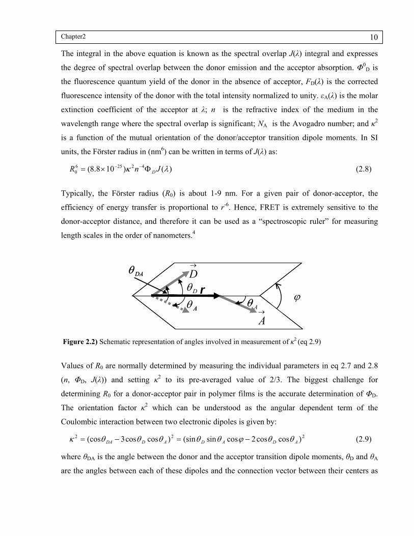
Coulombic interaction between two electronic dipoles is given by:
222 )coscos2cossin(sin)coscos3(cos ADADADDA (2.9)
where θDA is the angle between the donor and the acceptor transition dipole moments, θD and θA
are the angles between each of these dipoles and the connection vector between their centers as
DA
D
AD r
AA
DA
D
AD r
AA
Figure 2.2) Schematic representation of angles involved in measurement of κ2 (eq 2.9)

Chapter2
11
depicted in Figure 2.2. The separation angle φ, is the angle between the projections of the
transition moments on the plane perpendicular to the line through their centers.
In principle, the orientation factor κ2 can take values from 0 (perpendicular transition moments)
to 4 (collinear transition moments). For parallel transition moments κ2 = 1. For rapidly
reorienting dipoles, a situation typical of dilute solutions, (<κ2>), the average value of κ2, is 2/3.
In a rigid medium and for a random ensemble of donors and acceptors medium, κ2 = <κ>2 =
0.476.3
Usually, it is preferred to report R0 as a property of a donor-acceptor pair and in a way that is
independent of the rigidity of the medium. Therefore, reported R0 values are calculated with the
assumption of κ2 = 2/3 and are valid for systems in which molecules are free to rotate at a rate
much faster than the decay rate. For other conditions, i.e. rigid medium or when dipoles have a
particular orientation, one has to define R0,eff :
60
26,0 )
2
3( RR eff (2.10)
where the 3/2 cancels the 2/3 and κ2 corresponds to the specific experiment. Thus eq 2.6 can be
revised as:
6
02
2
3)(
r
Rrw
D
(2.11)
The quantum efficiency of energy transfer ΦET denotes the fraction of photons absorbed by the
donor that are transferred (nonradiatively) to the acceptor. For a donor-acceptor pair separated by
a distance r, the efficiency of energy transfer is given by:
660
60
)(/1
)(
rR
R
rw
rw
DET
(2.12)
When fluorophores are separated by a distance equal to R0, ΦET takes a value of 0.5. Typically,
the transfer efficiency is measured by comparing fluorescent intensity or integrated decay rate of
the donor in the absence and presence of the acceptor. In this case, one assumes that the decrease
in the fluorescent intensity of the excited donor or the increase in its fluorescence decay rate is
entirely due to energy transfer. Therefore ΦET can be written as:

Chapter2
12
D
DA
D
DA
ETdttI
dttI
1
)(
)(1 (2.13)
where τDA is the mean lifetime of the donor in the presence of acceptor and τD is the lifetime of
the donor in the absence of acceptor.
2.3 FRET in homogeneous systems
In section 2.2, resonance energy transfer between a single donor and acceptor separated by a
distance r was described in detail. This situation is typical of many biological systems in which
the molecules are labeled in specific sites and the rate of energy transfer reports the specific
distance between the two fluorophore. In most synthetic polymers and in my thesis, the dyes are
confined in domains and therefore one donor has the possibility to interact with several acceptors
located at different distances.
First, I will introduce a simple system in which donors are located in a medium with a
homogenous distribution of acceptors. Therefore, the acceptor concentration can be treated as
uniform over the space. For this system, Förster (1948) developed an equation for the time-
dependent intensity decay of donors.1
2
1)(exp)0()(
DD
tP
tItI
(2.14)
The above equation is known as Förster equation and is applicable for donor and acceptor
molecules randomly distributed in a volume that can be considered infinite on the scale of R0. In
this equation, the parameter P depends on the acceptor concentration and on the averaged
relative orientation κ2 of the donor and acceptor transition dipole moments and is expressed as:
AA CRNP 30
2/1223
2
3
3000
4 (2.15)
where CA is the acceptor concentration. The Förster equation provides a useful alternative means
for the determination of the Förster radius (R0). By preparing polymer films containing similar
donor concentrations with different acceptor concentrations and measuring their fluorescence
intensity decays, the P values for each sample can be determined from the fit of the fluorescence
intensity decays to the Förster equation.5 This treatment requires exponential donor decay in

Chapter2
13
polymer film in the absence of acceptor. According to eq 2.15, the P values obtained in this way
should have a linear relation with the acceptor concentration. Thus, the Förster radius (R0) can be
calculated from the slope of the linear fit using equation 2.15.5
2.4 FRET application in film formation processes
My approach for implementing FRET to study morphology of nanoparticles and film formation
behavior of aqueous dispersion heavily relies on models and assumptions. These assumptions are
necessary to analyze the data in an informative way. In this section I will explain different
approaches and the rationale I used to analyze fluorescence decay profiles. In all experiments
described in this thesis, I used a single FRET pair: a phenanthrene derivative as the FRET donor
and a benzophenone derivative as the FRET acceptors. Both of these derivatives carry a double
bond linker which enabled me to incorporate them via covalent bonds into the copolymer
backbone during free radical copolymerization. This way, the FRET dyes are side groups that are
located randomly along the copolymer backbone.
In the absence of NBen (acceptor), the phenanthrene (donor) decays exponentially in all the
copolymers I studied and the fluorescence lifetime (τD) was 44±1 ns. I found that the lifetime
depended slightly on the matrix in which the donor dye was incorporated. However, for each
copolymer I treated τD as constant during the study.
Most of my experiments are performed using a mixture of two aqueous dispersions that are
identical except that in one dispersion, polymer chains inside the nanoparticles are labeled with
the donor dye and in the other dispersion with the acceptor dye. I studied mixtures containing 10
wt% of donor- and 90 wt% of acceptor-labeled polymer. This ratio roughly translates into having
9 acceptor-labeled particles per donor-labeled particle. As water evaporates from films prepared
in this way, particles form a void free structure in which a donor-labeled particle is essentially
surrounded by acceptor-labeled particles. The mixing between polymer molecules inside these
particles could be followed by monitoring donor fluorescence decay profile. As diffusion and
mixing takes place, the average distance between donors and acceptor decreases, and thus w(r),
the rate of energy transfer, increases. Therefore, by measuring donor fluorescence decay profiles
periodically, we can capture the details of mixing and diffusion between labeled polymer
molecules. In what follows, I explain the experimental procedure I used to measure high

Chapter2
14
resolution fluorescence decay profiles. Then, I describe approaches that I used to convert these
fluorescence decay profiles into parameters that can describe the diffusion extent. Therefore, my
main goal is to relate the changes in w(r) and ΦET to the extent of mixing between polymer
molecules and the polymer diffusion rate.
2.5 Fluorescence intensity decay measurements
In my research, I used the time-correlated-singe-photon counting (TCSPC) technique to collect
donor fluorescence decay profiles. The TCSPC technique is based on the fact that for low level
high repetition rate signals, the light intensity at the detector is so low that the probability of
detecting one photon in one signal period is far less than unity. Thus, it is sufficient to record
photons and their arrival time in the signal period and build up a histogram of the photon times.
As a consequence, there are many excitation signal periods in which no photon is detected. Other
signal periods contain one photon detection pulse, and periods in which more that one photon is
detected are very rare.
In TCSPC, photon timing is performed by a time-to-amplitude-convertor (TAC). The excitation
source signal is fed to the TAC-stop, and the detector signal, to the TAC-start. This arrangement
is referred to as the reverse mode, as opposed to the forward mode in which one feeds the
excitation source signal to the TAC-start and the detector signal to TAC-stop. The reverse mode
is preferred for lifetime measurements, since it allows starting the TAC only on relatively rare
photon detection events, and affords more efficient use of TCSPC electronics. In the reverse
mode, the light source signal should be shifted by a delay to ensure that it arrives at the input of
the TAC later than the TAC-start signal. The TAC generates a signal whose amplitude is exactly
proportional to the time between the start and the stop pulse. The analogue signal of the TAC is
digitized by an analogue-to-digital-convertor (ATC) and then sent to a multichannel analyzer
(MCA). The resulting signal will provide the address (channel) in the memory of the MCA at
which the count has to be incremented by one.
High repetitive excitation sources include pico-second lasers, laser diodes (LD) and light
emitting diodes (LED). Single photon detection can be performed by a high gain detector such as
a photomultiplier or a micro-channel plate detector. In this thesis research, I used an LED as the

Chapter2
15
excitation source which produced nanosecond short pulses, and a micro-channel plate detector as
the photon detection module.
To measure a reliable decay profile, it is important to limit the photon detection events to one or
two photons per 100 incoming photons from the excitation source. In the reverse mode, emission
of a photon from a sample triggers the TAC and this photon is timed until an excitation photon is
generated by the light source. Other photons emitted by the sample during this time will not be
timed. If enough late photons are disregarded this way (pile-up effect) the measured decay is not
representative, and the measured lifetime will be shorter than the real lifetime. As a guideline,
pile-up is minimized by controlling the ratio of start-to-stop at a low value around 1-2%.
Measuring high resolution intensity decay profiles requires taking appropriate account of decay
distortions that originate from TCSPC instrumentation. Although fluorescence models and
analysis techniques are based on having narrow width (δ) excitation pulses, this condition is
hardly achievable experimentally. Having excitation pulses with a finite duration results in
distortion in the measured fluorescence decay (F(t)). Another source of decay distortion is the
lag time associated with counting photons in the TCSPC setup. The model (true) fluorescence
decay profiles (I(t)) do not contain information about the instrument response. Thus, (F(t)) and
(I(t)) cannot be compared directly.
Table 2.1 Notations used for referring to different types of fluorescence decay profile
F(t) Experimentally measured fluorescence decay profile on a sample of interest
I(t) Model (true) fluorescence decay profile
C(t) Experimentally measured fluorescence decay profile on a standard compound
IRF Instrument-response-function
A well-accepted method to correct for distortions caused by excitation pulse shape and delay
times associated with photon counting is to measure the instrument-response-function (IRF). IRF
is usually measured using a compound with a known and preferably very short lifetime. In my
research I used a mimic standard, a degassed solution of p-terphenyl which decays as a single
exponential with a lifetime of 0.96 ns.6 The experimentally measured decay on this solution
(C(t)) contains two types of information: p-terphenyl fluorescence information and information
pertaining to the IRF. In Table 2.1, I present a list of the notations used in this thesis to refer to

Chapter2
16
different types of fluorescence decay profiles. To obtain the true IRF, one considers that C(t) is
the result of a convolution integral between these two types of information as shown in eq 2.16.
Therefore, IRF can be recovered from C(t) following the procedure proposed by James et. al. 6
ds)/s(exp).s(IRF)/texp(ds]/)st([exp)s(IRF)t(Ct
0
t
0
(2.16)
This equation is only valid for a sample with exponential fluorescence decay. The above
equation can be written in the discrete form as:
)/iexp()i(IRF)/jexp()j(Cj
i
(2.17)
where ω is the MCA time per channel and j is the channel index. Eq 2.17 results in the following
recursive relationship for C(t) which enables one to calculate the true IRF knowing the lifetime
of the standard compound (τ).
)/exp()1j(C)j(C)j(IRF
or
)j(IRF)/exp()1j(C)j(C
(2.18)
There are two approaches available in the literature to consider the instrument response function:
convolution and deconvolution. It is generally preferred to avoid deconvolution since it is an ill-
posed problem. It may have a smearing-out effect and lead to loss of information. Therefore, it
is preferred to convolute the model (true) decay (I(t)) with the IRF as shown in eq (2.19).
t
0
ds)st(I)s(IRF)t(I)t(IRF)t(F (2.19)
The parameters of the model decay profile (I(t)) are then optimized to attain the best match
between I(t) and the measured decay profile (F(t)) as will be described in section 2.6.1.
2.6 Calculation of energy transfer quantum efficiency
There are several ways to obtain polymer diffusion rates from FRET experiments. First I will
describe a model-free approach that is based on calculating energy transfer quantum efficiency,
ΦET, as a measure of the extent of mixing for polymer diffusing in the nascent film across

Chapter2
17
particle-particle boundaries. One can calculate ΦET values from the areas under the donor
fluorescence decay profiles (eq 2.20).
D
a
D
D
aET
tarea
dttI
dttI
t
)(1
)(
)(
1)(
0
0
0
(2.20)
Although one could use in principle numerical integration, it is preferred to fit the decay to an
appropriate equation and then to calculate the integral analytically. My experience shows that
this approach leads to more consistent results and is not prone to deviations caused by using
different numerical integration methods. Later, in Section 2.7, I describe a modeling procedure
that calculates diffusion coefficient based on the shapes of donor fluorescence decay profiles.
In the presence of acceptors, the fluorescence decay profile is no longer single exponential. The
shape of the decay curve contains important information about the details of non-radiative
energy transfer between donors and acceptors and their distribution in the film. As explained in
section 2.3, for a uniform distribution of donors and acceptors in 3D space, the intensity of the
decay measured after δ-pulse excitations can be described by the Förster model (eq. 2.14) in
which P depends on the acceptor concentration (eq. 2.15) and the orientation factor (2 ) is
known to be 0.476 for random distribution of immobile chromophores in 3D space, a situation
typical for dyes embedded in polymer matrices.7
As diffusion proceeds, the volume fraction of regions that contain only donor-labeled polymer
decreases. However, domains of pure donors (with single exponential decay) exist until very late
stages of the interdiffusion process. Therefore, the decays no longer fit to the Förster model (a 2-
parameter equation). For this situation, we used the following empirical 3-parameter equation:
)t
exp(A)t
(At
expA)t(ID
32
1
D2
D1DA
(2.21)
To obtain A1, A2 and A3, the experimentally measured decay profiles were fitted to eq. 2.21 using
a nonlinear least square algorithm. Using the optimized fitting parameters enables one to
calculate the area under decay analytically within ca. 1% error. Despite its simplicity, eq 2.21 has
served us well as an empirical equation to fit donor fluorescence decay profiles with high

Chapter2
18
precision. Analyzing fluorescence data in terms of ΦET values, we could follow several aspects of
polymer diffusion such as the effects of latex composition5, polymer chain architecture,8
annealing temperature 5,9,10 and addition of various small molecules 11 on polymer diffusion rate.
Historically, eq 2.21 has its origin in an overly simplified idea about describing the mixing of
donor and acceptor-labeled polymers during film formation. The equation is composed of an
exponential terms and a Förster term (eq 2.14). It was assumed that the Förster term was due to
donors located in the mixed regions that can be treated with a single effective acceptor
concentration and the exponential term came from contribution of donors in the acceptor-free
regions (eq 2.5). As donor- and acceptor-labeled polymers mix, there is a concentration profile
which is far from a uniform distribution of acceptors in space, especially at the early stages of the
mixing process. For simplicity, it was assumed that acceptor containing regions can be
represented by a single concentration. With this simplifying assumption, one could use the
Fӧrster model to account for contribution of the mixed regions to the fluorescence signal. This is
not a good assumption and the prefactors A1 and A2 are not proportional to the volume fraction of
mixed- and pure-donor-regions and thus cannot be used directly to deduce mixing fraction.
2.6.1 Fitting experimental data
When donor fluorescence decay profiles were fitted to eq 2.21, τD was fixed to the donor lifetime
in the absence of acceptor and A1, A2 and A3 were treated as fitting parameters. There are several
approaches to analyze fluorescence decay curves.12 I obtained the fitting parameters by
minimizing χ2 as the objective function using a nonlinear least square analysis. χ2 is defined
based on the squared residuals, the square of the difference between the experimentally obtained
value and the value calculated from eq 2.21 with a given set of parameters (A1, A2 and A3). The
difficulty is that even for an exponential (the simplest decay model), the objective function
defined in this way contains a square of an exponential and becomes nonlinear. Thus, an
analytical solution is not possible and trial and error minimization algorithms should be used. A
common problem with all these algorithms is that they are prone to trapping by local minima in
the objective function surface and hence the fitting procedure might find only local minima.
Minimization algorithms vary the fitting parameters stepwise to minimize the objective function.
Descent gradient methods are the simplest and the most popular minimization algorithms in

Chapter2
19
which the parameters are changed by a step size proportional to the negative of the objective
function gradient. This method loses applicability when dealing with multi-parameter nonlinear
objective functions for which the shape of the objective function versus fitting parameters can be
very irregular. Following descent gradient methods, one essentially takes big steps when close to
a local minimum of the objective function. In practice, this is where we want to take small steps
not to miss the minimum. On the other hand, when moving on a gently sloped part of objective
function, the descent gradient dictates taking small steps whereas in practice one needs to take
big steps to reduce the convergence time. Hence, such procedures have found limited
applicability for stiff problems such as fitting fluorescence decay data.
To speed up convergence, one needs to estimate the shape of the objective function (χ2) vs.
fitting parameters and develop a method to determine step size based on local steepness of this
curve. Therefore, not only the objective function but also the first and second derivative of the
objective function needs to be estimated with respect to the parameters. In this way, the
minimization algorithm determines the step size by combining the curvature of the objective
function (second order information) with its gradient (first order information).
For my data analysis, I selected the Levenberg-Marquardt optimization algorithm. The basic idea
behind this method is that close to a minimum, the shape of the objective function can be
approximated by a quadratic function. Therefore, it follows that close to a minimum the shape of
the function to be fitted (e.g. eq 2.21) can be approximated by a linear function. This way, the
objective function (sum of squared residuals) takes a quadratic form for which we can arrive to
the approximate minimum analytically.
In the Levenberg-Marquardt optimization algorithm, the appropriate step size is determined by
carefully blending the gradient of the objective function weighted by a suitable prefactor with
curvature information. For each set of fitting parameters, the curvature information can be
estimated using the quadratic shape assumption explained above. First, the objective function is
evaluated for a set of fitting parameters. Then the algorithm changes the fitting parameters to
minimize the objective function. If the error is increasing, then the step is rejected and the
algorithm increases the prefactors of the gradient information. The intuition is that if the error
increases, the objective function is not close to a minimum, and the quadratic approximation is
not working well. Therefore, we have to decrease its weight by increasing the prefactors of the
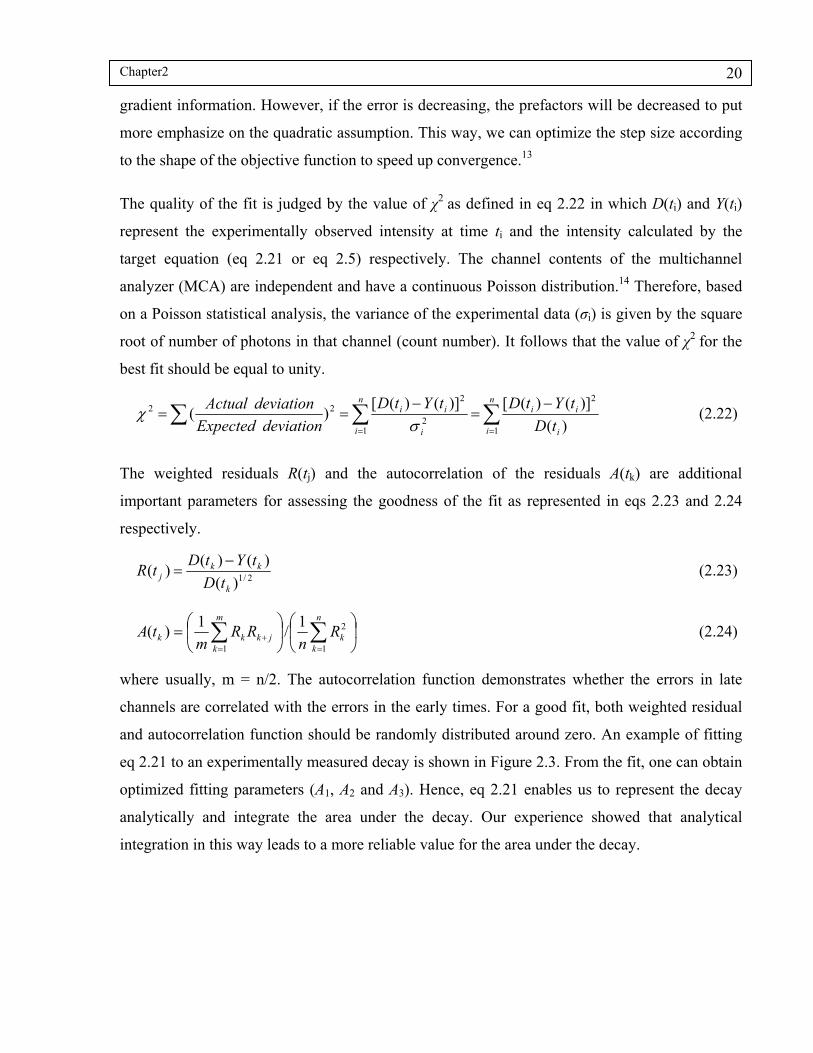
Chapter2
20
gradient information. However, if the error is decreasing, the prefactors will be decreased to put
more emphasize on the quadratic assumption. This way, we can optimize the step size according
to the shape of the objective function to speed up convergence.13
The quality of the fit is judged by the value of χ2 as defined in eq 2.22 in which D(ti) and Y(ti)
represent the experimentally observed intensity at time ti and the intensity calculated by the
target equation (eq 2.21 or eq 2.5) respectively. The channel contents of the multichannel
analyzer (MCA) are independent and have a continuous Poisson distribution.14 Therefore, based
on a Poisson statistical analysis, the variance of the experimental data (σi) is given by the square
root of number of photons in that channel (count number). It follows that the value of χ2 for the
best fit should be equal to unity.
n
i i
iin
i i
ii
tD
tYtDtYtD
deviationExpected
deviationActual
1
2
12
222
)(
)]()([)]()([)(
(2.22)
The weighted residuals R(tj) and the autocorrelation of the residuals A(tk) are additional
important parameters for assessing the goodness of the fit as represented in eqs 2.23 and 2.24
respectively.
2/1)(
)()()(
k
kkj tD
tYtDtR
(2.23)
n
kk
m
kjkkk R
nRR
mtA
1
2
1
1/
1)( (2.24)
where usually, m = n/2. The autocorrelation function demonstrates whether the errors in late
channels are correlated with the errors in the early times. For a good fit, both weighted residual
and autocorrelation function should be randomly distributed around zero. An example of fitting
eq 2.21 to an experimentally measured decay is shown in Figure 2.3. From the fit, one can obtain
optimized fitting parameters (A1, A2 and A3). Hence, eq 2.21 enables us to represent the decay
analytically and integrate the area under the decay. Our experience showed that analytical
integration in this way leads to a more reliable value for the area under the decay.

Chapter2
21
Time (ns)
Inte
nsi
ty (
cou
nts
)
105
104
103
102
10
00 50 100 150 200 250
Lamp
250
Re
sid
ua
ls
-4
4
0
250
-0.6
0.6
0
Au
toc
orr
ela
tio
n
Fu
nc
tio
n
Time (ns)
Inte
nsi
ty (
cou
nts
)
105
104
103
102
10
00 50 100 150 200 250
Lamp
250
Re
sid
ua
ls
-4
4
0
250
-0.6
0.6
0
Au
toc
orr
ela
tio
n
Fu
nc
tio
n
A)
B)
C)
Time (ns)
Inte
nsi
ty (
cou
nts
)
105
104
103
102
10
00 50 100 150 200 250
Lamp
250
Re
sid
ua
ls
-4
4
0
250
-0.6
0.6
0
Au
toc
orr
ela
tio
n
Fu
nc
tio
n
Time (ns)
Inte
nsi
ty (
cou
nts
)
105
104
103
102
10
00 50 100 150 200 250
Lamp
250
Re
sid
ua
ls
-4
4
0
250
-0.6
0.6
0
Au
toc
orr
ela
tio
n
Fu
nc
tio
n
A)
B)
C)
Figure 2.3) A) Example of fitting fluorescence decay profile to eq 2.22 using Levenberg-Marquardt algorithm. The weighted residuals (B) and the autocorrelation function (C) appears randomly distributed around zero. The χ2 was 1.06 for this fit.
2.6.2 Polymer diffusion coefficient
To capture the diffusion between donor- and acceptor-labeled polymers, I measured fluorescence
decays on a film cast from a mixture of donor- and acceptor-labeled particles with a ratio of 1/9.
During annealing of this film several decays were measured periodically and fitted to eq 2.21.
The quantum efficiency of energy transfer at each annealing time ΦET(ta) were then calculated
according to eq 2.20:
D
a
D
D
aET
tarea
dttI
dttI
t
)(1
)(
)(
1)(
0
0
0
(2.20)
Chapter2
22
As donor- and acceptor-labeled chains diffuse together, the rate of energy transfer increases.
Therefore, the decay becomes more curved and the area under the decay decreases. One can
think of the area under the decay as an average donor lifetime at each annealing time.
From the values of ΦET as a function of annealing time, we calculated values of the fraction of
mixing (fractional growth in energy transfer):
)0()(
)0()()(
ETET
ETaETam
ttf
(2.25)
where ΦET(0) and ΦET(∞) represents the initial and final values of energy transfer. The
numerator describes the difference in energy transfer of a nascent film just after particle
coalescence and a film annealed for time ta, and the denominator represents the energy transfer
difference between a nascent film and a fully mixed film. If particle coalescence and polymer
diffusion happen on very different time scales, there is still a limited amount of energy transfer in
the nascent film. Donors and acceptors located on different sides of the sharp particle boundaries
are close enough (on the scale of R0) to undergo energy transfer. In the past, our group used a
value of 0.07 for nascent films prepared from particles around 150 nm in diameter.15,16 In
practice, films dry from the edges inward and some diffusion takes place before the first decay is
measured. For polymers with a significant enough diffusion rate, the value of ΦET(0) is not
experimentally accessible and we have to rely on calculations as will be described in the next
section. Besides diffusion, surface roughness of the particle-particle interfaces in the nascent film
can lead to ΦET values which are larger than the calculated ΦET(0).17
ΦET(∞) is the value of energy transfer for a film in which acceptor-labeled polymer is
homogenously diluted by donor-labeled polymer. To obtain this value experimentally, I
dissolved the dried latex mixture in tetrahydrofuran (THF) to make a dilute solution (ca. 5
mg/ml) and then cast a film from this solution. ΦET(∞) was obtained from a decay measured on
this film after complete evaporation of THF. I could fit such decays to the Förster equation (eq
2.14) and obtained ΦET(∞) values using eq 2.13.
To obtain an apparent diffusion coefficient (Dapp) we need to make further assumptions. First,
although the honeycomb-like structure formed after coalescence in the nascent film is composed
of closed-packed dodecahedra, for calculation simplicity, I chose to treat cells formed by the

Chapter2
23
donor-labeled particles as spheres. Second, we assumed that the “quantum fraction” of mixing
(fm) as defined by eq 2.25 can be used to represent the mass fraction of mixing (fs). Third, the
mechanism of diffusion is assumed to be Fickian. We used Fick’s law to describe diffusion in a
core-shell geometry that consists of a particle with radius R containing donor-labeled polymers
and a shell of acceptor-labeled polymer. The radius of the donor-labeled particles (R) in
dispersion and prior to film formation was determined by dynamic light scattering (DLS). The
shell was assumed to be infinitely thick. The fraction of polymer molecules that have diffused
out of the core at time t is given by:
R
m drrtrCR
f0
23
4),(4
31
(2.26)
where C(r,t) is the normalized concentration profile of donors at annealing time ta. A common
practice is to use the initial concentration of the dye (C0) to normalize C(r,t). 18 Solving Fick’s
second law in the core-shell geometry results in the following equation for C(r,t) 19
})2
(exp[
])2
(){exp[()]2
()2
([2
),(
}2
200
x
rRx
rRx
r
C
x
rRerf
x
rRerf
CtrC
(2.27)
where x represents the extent of diffusion ( tDx app. ) and erf is the error function.
Thus by measuring fm as a function of annealing time, one can calculate values of apparent
diffusion coefficient (Dapp) using equations 2.26 and 2.27. 20 Dapp values obtained in this way are
cumulative mean diffusion coefficients. In other words, at each annealing time, Dapp is the
weighted average of the diffusion coefficients of all species that have diffused up to that time.
These Dapp values are not true center of mass diffusion coefficients but are proportional to those
values (see below).
Although eq 2.21 served us well in fitting donor fluorescence decay profiles and calculating the
area under the decays, it does not afford a rigorous theoretical identification of mixed and
unmixed regions. Several attempts at taking explicit account of the concentration profiles in
fitting ID(t) has been made. For example Liu et al. from our group21 and also Dhinojwala from
the Torkelson group22 attempted to take account acceptor concentration profiles generated by
diffusion. The concentration profiles were calculated based on a Fickian diffusion model and

Chapter2
24
were then subdivided into infinitesimally small slices. It was assumed that the acceptor
concentration can be treated as constant within each slice. The fluorescence intensity is obtained
by summing over the donor fluorescence in all slices.
Farinha et al. from our group pointed out that, in the above approaches, one has to assume that
each donor is restricted to a region with a uniform acceptor concentration. Therefore, although
the above mentioned models are closer to reality, they are still based on the assumption that the
acceptor concentration is constant over infinitesimally small slices. Proper consideration of the
donor and acceptor concentration profile requires evaluating energy transfer kinetics in restricted
geometries for which at least one dimension is comparable to R0. Farinha et al. related the
fluorescence intensity to the survival probability of donors. Based on the formalism developed
by Klafter and Blumen, the survival probability of donor depends on the acceptor concentration
profile.23 A Fickian diffusion model was used to drive the concentration profile of the acceptors.
The calculations by Farinha et. al showed that fm is larger than the mass fraction of mixing (fs)
but fm and fs are proportional for fm values below 0.7. 15 They demonstrated that for fm values
below 0.7, estimation of fs by fm results in higher Dapp values that are larger by a factor of 2-3
compared to the averaged center of mass diffusion coefficients. At higher fm values, using fm
instead of fs can overestimate the diffusion coefficient by more than an order of magnitude.
In what follows, I will explain my approach for using concentration profiles obtained from
Fick’s second law to calculate model fluorescence decay profiles appropriate to specific
annealing times (or diffusion extents). This approach is based on Monte Carlo sampling of the
normalized concentration profile.
2.7 Monte Carlo calculations of energy transfer
Monte Carlo (MC) algorithms are a class of computational methods that provide an approximate
solution to a complex problem via random sampling. Random sampling is performed using
computer generated random numbers. MC methods have been used extensively for solving
transport phenomena problems. 24,25 Enhanced computational power offered by new central
processing units (CPUs) has paved the way for using this technique in more complex geometries.

Chapter2
25
Shell (A)
Core (D)
Extended acceptor shell(5R0 in Thickness) Shell (A)
Core (D)
Extended acceptor shell(5R0 in Thickness) Shell (A)
Core (D)
Extended acceptor shell(5R0 in Thickness)
Figure 2.4) Schematic representation of the core-shell geometry used for Monte Carlo calculations of energy transfer efficiency.
I used normalized donor and acceptor concentration profiles as probability density functions to
generate ensembles of donors and acceptors by a Monte Carlo sampling technique. Virtual
donors and acceptors were placed in the core-shell geometry using a random number generator.
A schematic representation of the core-shell geometry is represented in Figure 2.4. In this
geometry, a donor-labeled particle (Rp in radius) is located in the core and is surrounded by an
acceptor-labeled shell. The thickness of the shell was adjusted in such a way that the core
volume fraction was equal to the volume fraction of donor-labeled particles used to prepare the
film. Therefore, unlike the previous model, here the thickness of the acceptor shell is finite and
the volume fraction of acceptors in the simulation box is determined according to the
experimental conditions. The net mass flux across the outer boundary of the shell was set to zero
throughout the calculations. For this geometry, according to the assumption of Fickian diffusion,
the normalized donor- and acceptor-concentration as a function of distance from the particle
center (r) and extent of diffusion (x, x2 = Dt) is given by:19
n
pnp
2n
pn
1n n2
n2n
2
3
3p
D α
)Rcos(αR
α
)Rsin(α
a)(αsin
r)sin(α)αxexp(
r.a
2
a
R(r,t)C (2.28)
where r is the distance from the particle center, a is the outer shell radius and the extent of
diffusion x is given by x2 = Dt. From the mass balance, it follows that the acceptor concentration
profile is given by:
(r,t)C1(r,t)C DA (2.29)
In these expressions, t is the annealing (aging) time and αn are the positive roots of the equation:
1)cot(aαaα nn (2.30)
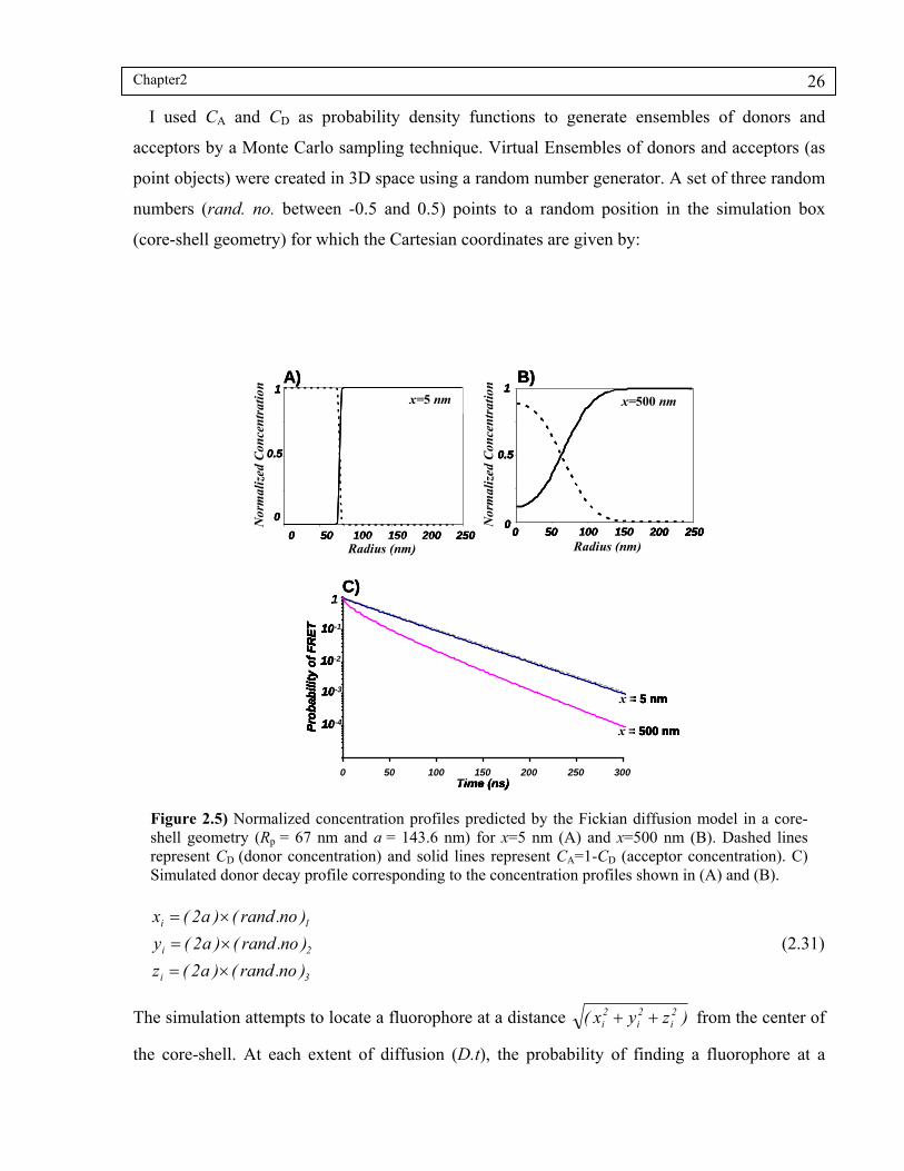
Chapter2
26
I used CA and CD as probability density functions to generate ensembles of donors and
acceptors by a Monte Carlo sampling technique. Virtual Ensembles of donors and acceptors (as
point objects) were created in 3D space using a random number generator. A set of three random
numbers (rand. no. between -0.5 and 0.5) points to a random position in the simulation box
(core-shell geometry) for which the Cartesian coordinates are given by:
3i
2i
1i
)no.rand()a2(z
)no.rand()a2(y
)no.rand()a2(x
(2.31)
The simulation attempts to locate a fluorophore at a distance )zyx( 2i
2i
2i from the center of
the core-shell. At each extent of diffusion (D.t), the probability of finding a fluorophore at a
Nor
mal
ized
Con
cen
trat
ion
Radius (nm)
x=500 nm
0
0.5
1
0 50 100 150 200 250
B)x=5 nm
Nor
mal
ized
Con
cen
trat
ion
Radius (nm)
0
0.5
1
0 50 100 150 200 250
A)
0 50 100 150 200 250 300Time (ns)
Pro
bab
ilit
y o
f F
RE
T
1
10-1
10-2
10-3
10-4
x = 5 nm
x = 500 nm
0 50 100 150 200 250 300Time (ns)
Pro
bab
ilit
y o
f F
RE
T
1
10-1
10-2
10-3
10-4
x = 5 nm
x = 500 nm
C)
Nor
mal
ized
Con
cen
trat
ion
Radius (nm)
x=500 nm
0
0.5
1
0 50 100 150 200 250
B)
Nor
mal
ized
Con
cen
trat
ion
Radius (nm)
x=500 nm
0
0.5
1
0 50 100 150 200 250
Nor
mal
ized
Con
cen
trat
ion
Radius (nm)
x=500 nm
0
0.5
1
0 50 100 150 200 250
B)x=5 nm
Nor
mal
ized
Con
cen
trat
ion
Radius (nm)
0
0.5
1
0 50 100 150 200 250
A)x=5 nm
Nor
mal
ized
Con
cen
trat
ion
Radius (nm)
0
0.5
1
0 50 100 150 200 250
A)
0 50 100 150 200 250 300Time (ns)
Pro
bab
ilit
y o
f F
RE
T
1
10-1
10-2
10-3
10-4
x = 5 nm
x = 500 nm
0 50 100 150 200 250 300Time (ns)
Pro
bab
ilit
y o
f F
RE
T
1
10-1
10-2
10-3
10-4
x = 5 nm
x = 500 nm
C)
0 50 100 150 200 250 300Time (ns)
Pro
bab
ilit
y o
f F
RE
T
1
10-1
10-2
10-3
10-4
x = 5 nm
x = 500 nm
0 50 100 150 200 250 300Time (ns)
Pro
bab
ilit
y o
f F
RE
T
1
10-1
10-2
10-3
10-4
x = 5 nm
x = 500 nm
C)
Figure 2.5) Normalized concentration profiles predicted by the Fickian diffusion model in a core-shell geometry (Rp = 67 nm and a = 143.6 nm) for x=5 nm (A) and x=500 nm (B). Dashed lines represent CD (donor concentration) and solid lines represent CA=1-CD (acceptor concentration). C) Simulated donor decay profile corresponding to the concentration profiles shown in (A) and (B).
Chapter2
27
given radial position (Pr) is given by eq 2.28 as plotted in Figure 2.5A and B. To place a
fluorophore, another random number (rand. no.4) was generated and compared with Pr. The
fluorophore was placed on the simulation box only if 4r .no.randP . In this case, the Cartesian
coordinates were saved for further calculations.
Donors may be placed within a distance a of the particle center. To ensure that the energy
transfer from the donors located near the outer boundary is properly taken into account, an
additional layer containing acceptors (5R0 in thickness) with a concentration of CA(a) was added
to the outer shell (Figure 2.4). Based on eq. 2.11, the rate of energy transfer can be shown to be
negligible for a donor and an acceptor apart by more than 5R0. Based on this modification,
acceptors may be placed with a distance a+5R0 from the particle center.
I increased the number of donor dyes until the results (the calculated decays) were independent
of the actual number of donors. Therefore, the number of donors was large enough to guarantee
the statistical stability of the model. The number of acceptors was determined based on the
experimental conditions: labeling density of acceptor-labeled polymer, weight ratio of acceptor
polymer and polymer density. Following this procedure a population of virtual donors and
acceptors were built in the core-shell geometry that resembles the normalized concentration
profile at each D.t.
The simulation calculates the distance between every donor in the simulation box and the
acceptors using the Cartesian coordinates of the fluorophores. A unit vector with random
orientation is generated for the donor and acceptor pairs that are located closer than 5R0. In this
way, for each donor and acceptor pair the distance (r) and the orientation factor (kij) are known.
The decay (ID(t’)) from such ensemble of fluorophore is given by summing the contribution of
all donors to the fluorescence signal as shown in eq 2.32. 26,27
D AN
1j
N
1k
6
jk
o2jk
DDDD/A r
Rκ
2
3
τ
texp
τ
texp
N
1)t(I (2.32)
The quantum efficiency of energy transfer (ΦET) is given by:

Chapter2
28
D AN
1j
1N
1k
6
ij
02ij
DET r
Rκ
2
31
N
11Φ (2.33)
where NA and ND are the number of acceptors and donors in the system.
I generated a series of donor decay profiles representing increasing extents of diffusion (x). As
diffusion progresses, the average distance between donors and acceptors decreases and therefore
the rate of energy transfer increases (Figure 2.5C).
The trial ID/A(t’) profiles were convoluted with the instrument response function (IRF)
corresponding to each specific experiment (eq 2.19) and then compared through a fitting analysis
to the experimentally measured decay profile (F(t)). In this case, the fitting analysis is straight
forward as all we need to do is to minimize the sum of squared differences between the measured
and the calculated intensities over all channels. For the best fit, values of the χ2 parameter were
between 0.95 and 1.2, and the plots of weighted residuals and the autocorrelation function of
weighted residuals were randomly distributed around zero. The diffusion coefficient was
calculated by dividing x2 by the annealing time (t). The simulation analysis assumes that a mean
value of Dapp describes the Fickian diffusion that has taken place over all times up to t.
0
0.1
0.2
0.3
0.4
0.5
0.6
0.7
0 250 500 750 1000x (nm)
ΦE
T
0
0.1
0.2
0.3
0.4
0.5
0.6
0.7
0 250 500 750 1000x (nm)
ΦE
T
Figure 2.6) Evolution of the energy transfer efficiency (ΦET) calculated from simulated decays in a core-shell geometry (Rp = 67 nm and a = 143.6 nm) as Fickian diffusion proceeds (increasing extent of diffusion, x).

Chapter2
29
x= (
D.t)
1/2
(nm
)
0
100
200
300
400
0 10 20 30 40
t1/2 (min)1/2
40 °C
50 °C
60 °C
70 °C
x= (
D.t)
1/2
(nm
)
0
100
200
300
400
0 10 20 30 40
t1/2 (min)1/2
40 °C
50 °C
60 °C
70 °C
Figure 2.7) Plots of the extent of diffusion vs square root of time at four annealing temperatures. The lines are best-fitted lines to the data points. The linear relation between x and t1/2 points to a Fickian diffusion mechanism.
The fractional growth in quantum efficiency of energy transfer (ΦET) was calculated using eq
2.33. ΦET(0) was taken as the calculated value for energy transfer quantum efficiency at D.t = 0.
One anticipates that the system will become fully mixed at high extents of diffusion, with ΦET
reaching a plateau. This behavior was followed in the simulations as shown in Figure 2.6. For
particles around 150 nm in diameter used in my studies, I found that the values of ΦET(∞) can be
estimated as the ΦET obtained for x = 1000. After x=1000, increasing the extent of diffusion had
negligible effects on the calculated ΦET value.
Figure 2.7 represents the evolution in the extent of diffusion (x) for a P(BA50MMA49) sample at
four different annealing temperatures, namely 40, 50, 60 and 70 °C. At each temperature, the
experimental data points were obtained by periodically measuring donor fluorescence decay
profile of the film which had been annealed at that temperature. These decay profiles were then
analyzed according to the procedure described in this section to calculate the extent of diffusion
(x). In Figure 2.7, the dashed lines are the best fits to the experimental data. As one can observe,
there is a linear relation between x and t1/2 which is a characteristic of Fickian diffusion.
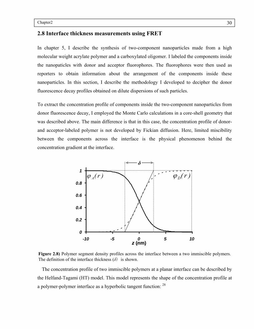
Chapter2
30
2.8 Interface thickness measurements using FRET
In chapter 5, I describe the synthesis of two-component nanoparticles made from a high
molecular weight acrylate polymer and a carboxylated oligomer. I labeled the components inside
the nanopaticles with donor and acceptor fluorophores. The fluorophores were then used as
reporters to obtain information about the arrangement of the components inside these
nanoparticles. In this section, I describe the methodology I developed to decipher the donor
fluorescence decay profiles obtained on dilute dispersions of such particles.
To extract the concentration profile of components inside the two-component nanoparticles from
donor fluorescence decay, I employed the Monte Carlo calculations in a core-shell geometry that
was described above. The main difference is that in this case, the concentration profile of donor-
and acceptor-labeled polymer is not developed by Fickian diffusion. Here, limited miscibility
between the components across the interface is the physical phenomenon behind the
concentration gradient at the interface.
The concentration profile of two immiscible polymers at a planar interface can be described by
the Helfand-Tagami (HT) model. This model represents the shape of the concentration profile at
a polymer-polymer interface as a hyperbolic tangent function: 28
0
0.2
0.4
0.6
0.8
1
-10 -5 0 5 10z (nm)
)r(A )r(D
δ
0
0.2
0.4
0.6
0.8
1
-10 -5 0 5 10z (nm)
)r(A )r(D
δ
Figure 2.8) Polymer segment density profiles across the interface between a two immiscible polymers. The definition of the interface thickness (δ) is shown.

Chapter2
31
)z(1)z(
))z2
tanh(1(2
1)z(
AB
A
(2.34)
Here φ is the volume fraction of components across the interface and z is the distance with
respect to the center of the interface region (Figure 2.8). The definition of δ is somewhat
arbitrary. In the HT model, the interface thickness (δ) is defined using the tangent of φ(z) profiles
at z=0: 28
0zA )z(
1
(2.35)
The above definition became well-accepted and was widely used in subsequent publications of
other groups. 29,30 This definition leads to a simple geometrical interpretation of δ as delineated in
Figure 2.8. If one draws the tangent of the concentration profile at z=0 and extends it to the z
axis, the base of the triangle formed in this way is equal to δ/2.
To proceed with the MC calculations, the concentration of labeled polymers across the spherical
interface in the core-shell geometry is needed. In this geometry, the normalized concentration of
donors (CD(r)) and acceptors (CA(r)) according to the HT model can be written as:31
)r(C1)r(C
])/)Rr(2tanh[1)(2
1()r(C
AD
sA
(2.36)
Here Rs is the radius of the core particles and δ is the interface thickness as defined previously.
The value of the interface thickness is a measure of interpenetration at the interface and depends
on the thermodynamic interactions between polymers across the interface. The sharp interface
between two immiscible polymers is characterized by a small δ value. The simulation procedure
was similar to what was described in the previous section. The only difference is that here, eq
2.36 was used to generated the ensemble of donors and acceptors in the core-shell geometry.
Since in these experiments, the shell polymer is labeled with the donor dyes, adding an
additional layer of acceptor-labeled polymer was not necessary.
Figure 2.9A represents a series of concentration profiles generated using Rs = 55 nm and a
particle radius (Rp ) of 78 nm. As the interface thickness increased, the average distance between
donors and acceptor decreased and thus the rate of energy transfer increased. As shown in Figure

Chapter2
32
2.9B, the area under simulated decay decreased as δ increased. From the simulations, I calculated
values of ΦET (eq 2.33). Figure 2.10 shows the evolution of ΦET as the interface thickness was
increased for a particular core-shell geometry with Rs = 55 nm and Rp = 78 nm.
0 50 100 150 200 250
Time (ns)
Pro
bab
ilit
y o
f F
RE
T
1
10-1
10-2
10-3
δ = 20 nmδ = 0 nm
δ = 5 nm
0 50 100 150 200 250
Time (ns)
Pro
bab
ilit
y o
f F
RE
T
1
10-1
10-2
10-3
δ = 20 nmδ = 0 nm
δ = 5 nm
0
0.2
0.4
0.6
0.8
1
0 15 30 45 60 75 90
r (nm)
CA Rs
δ (nm): 0
520
0
0.2
0.4
0.6
0.8
1
0 15 30 45 60 75 90
r (nm)
CA Rs
δ (nm): 0
520
A)
B)
Figure 2.9) A) radial distribution function of acceptor-labeled polymer for core-shell particles with Rs = 55 nm and Rp = 78 nm with three different interface thickness (δ). B) Simulated donor decay profile corresponding to the concentration profiles shown in (A).

Chapter2
33
2.9 Summary
In this chapter, I described the basic principles of the fluorescence resonance energy transfer
(FRET) and its application to the study of latex film formation. FRET is a powerful technique for
obtaining information about the distribution of polymer molecules labeled with donors and
acceptors. This technique is relatively easy to implement, and it offers a remarkable spatial
resolution. However, to interpret the data in a meaningful way, one needs to implement
quantitative models. This is a common challenge for all experimental techniques that indirectly
measure diffusion coefficient of polymers such as small angle neutron scattering (SANS). I
presented the rationale and approaches I used to analyze donor fluorescence decay profiles.
These analysis techniques enabled me to obtain quantities that describe diffusion during film
formation. Two important parameters include the mixing fraction and the apparent diffusion
coefficient.
0
0.1
0.2
0.3
0 20 40 60δ (nm)
ΦE
T
0
0.1
0.2
0.3
0 20 40 60δ (nm)
ΦE
T
Figure 2.10) Values of energy transfer efficiency (ΦET) calculated from simulated decays in a core-shell geometry (Rs = 55 nm and Rp = 78 nm) for various interface thicknesses (δ).

Chapter2
34
2.10 References
1 Förster, T. Annalen der Physik 1948, 437, 55-75.
2 Becker, W. Advanced Time-Correlated Single Photon Counting Techniques; Berlin: Springer, 2005.
3 Valeur, B. Molecular Fluorescence: Principles and applications. Wiley-VCH: New York, 2002.
4 Stryer, L.; Haugland R. P. Proc. Natl. Acad. Sci. U.S.A. 1967, 58, 719.
5 Liu, Y.; Haley, J. C.; Deng, K.; Lau, W.; Winnik, M. A. Macromolecules 2007, 40, 6422-6431.
6 James, D. R.; Demer, D.; Verrall, R.; Steer, R. Rev. Sci. Instrum. 1983, 54, 1121.
7 Lakowicz, J. R. Principals of fluorescence spectroscopy; third edition, Berlin: Springer, 2006.
8 Liu, Y.; Schroeder, W. F.; Haley, J. C.; Lau, W.; Winnik, M. A. Macromolecules 2008, 41,
9104-9111.
9 Soleimani, M.; Haley, J. C.; Lau, W.; Winnik, M. A. Macromolecules 2010, 43, 975-985.
10 Oh, J. K.; Tomba, P.; Ye, X.; Eley, R.; Rademacher, J.; Farwaha, R.; Winnik, M. A.
Macromolecules 2003, 36, 5804-5814.
11 Schroeder, W. F.; Liu, Y.; Tomba, J. P.; Soleimani, M.; Lau, W.; Winnik, M. A. J. Phys.
Chem. B 2010, 114, 3085-3094.
12 Lakowicz, J. R. Topics in Fluorescence spectroscopy, Volume 1, Techniques; Plenum Press,
New York, 1991.
13 Press, W. H.; Saul, A. T.; Vetterling, W. T.; Flannery, B. P. Numerical recipes in C, Cambridge University Press, second edition, NY, 2002.
14 O'Connor, D. V; Phillips, D. Time correlated single photon counting; Academic Press, Inc.
1984.
15 Farinha, J. P. S.; Martinho, J. M. G.; Yekta, A.; Winnik, M. A. Macromolecules 1995, 28, 6084-6088.

Chapter2
35
16 Liu, Y.; Schroeder, W.; Soleimani, M.; Lau, W.; Winnik, M. A. Macromolecules 2010, 43, 6438-6449.
17 Nakashima, K.; Liu, Y.; S. Zhang, P.; Duhamel, J.; Feng, J.; Winnik, M. A. Langmuir 1993, 9, 2825-2831.
18 Crank, J. The Mathematics of Diffusion, Clarendon Press, Oxford, 1975.
19 Crank, J. The Mathematics of Diffusion, Clarendon Press, Oxford, 1975.
20 Wang, Y.; Zhao, C.; Winnik, M. A. J. Chem. Phys. 1991, 95, 2143.
21 Liu, Y. S.; Feng, J.; Winnik, M. A. J. Chem. Phys. 1994, 101, 9096.
22 Dhinojwala, A.; Torkelson, J. M. Macromolecules 1994, 27, 4817-4824.
23 Klafter, J.; Blumen, A. J. Chem. Phys. 1984, 80, 875.
24 Miller, R. E.; Tadmore, E. B. J. Comput. Aided Mater. Des. 2002, 9, 203.
25 Kremer, K.; Muller Plathe, F. Mol. Simul. 2002, 28, 729.
26 Yang, J.; Winnik, M. A. J. Phys. Chem. B 2005, 109, 18408-18417.
27 Haley, C. J.; Liu, Y.; Winnik, M. A.; Demmer, D.; Haslett, T.; Lau, W. Rev. Sci. Instrum. 2007, 78, 084101.
28 Helfand, E.; Tagami, Y. J. Chem. Phys. 1972, 56, 3592.
29 Yekta, A.; Spiro, J. G.; Winnik, M. A. J. Phys. Chem. B 1998, 102, 7960-7970.
30 Shull, K. R.; Mayes, A. M.; Russell, R. P. Macromolecules 1993, 26, 3929-3936.
31 a) Farinha, J. P. S.; Vorobyova, O.; Winnik, M. A. Macromolecules 2000, 33, 5863-5873. b) Rharbi, Y.; Yekta, A.; Winnik, M. A.; DeVoe, R. J.; Barrera, D. Macromolecules 1999, 32, 3241-3248.

Chapter 3 36
CHAPTER THREE
Effect of Hydroplasticization on Polymer Diffusion in Poly (butyl
acrylate-co-methyl methacrylate) and Poly (2-ethylhexyl acrylate -
co- tert-butyl methacrylate) Latex Films i
3.1 Introduction
Plasticizing polymers by incorporating small molecules as additives is a common strategy for
modifying the mechanical properties of polymers.1 At the molecular level, plasticizers affect
intermolecular interactions and therefore chain relaxation dynamics by decreasing the internal
friction coefficient among polymer chains. In this context, a variety of different organic
compounds are intentionally introduced to polymer systems as plasticizers. For instance, in the
coatings industry, volatile organic compounds (VOC) are often added to aqueous polymer latex
formulations to decrease the modulus of polymer particles. In the presence of these volatile
plasticizers, the particles become soft enough to deform and pack to yield transparent and void-
free continuous films upon water evaporation. Over a longer time scale, as the VOCs escape to
the atmosphere, the glass transition temperature (Tg) of the polymer film increases, and the film
hardness improves.
Hydroplasticization, plasticization by moisture, often occurs unintentionally since water has
limited but non-negligible solubility in many polymers. Despite its poor miscibility, moisture can
lead to dramatic changes in the mechanical properties of a polymer. Hydroplasticization is more
prominent for applications in which polymers are exposed to water-rich media such as body
fluids (e.g. tablet coatings, drug delivery systems, and implants) 2- 5 or ambient moisture (e.g.
polymer adhesives, automotive parts, latex paints and coatings).6- This problem is accentuated in
water-based paints since they often contain salts and other hydrophilic additives.8
i This chapter appeared as: “Effect of Hydroplasticization on Polymer Diffusion in Poly(butyl acrylate-co-methyl methacrylate) and Poly(2-ethylhexyl acrylate-co-tert-butyl methacrylate) Latex Films” Soleimani, M.; Haley, J.; Lau, W.; Winnik, M. Macromolecules 2010, 43, 975-985.

Chapter 3 37
Moisture absorption into a polymer matrix is driven by osmotic pressure and proceeds until the
activity of water absorbed into the polymer is equal to that in the vapor phase. For glassy
polymers such as epoxy resins, the swelling stress may cause irreversible physical damage such
as microcracking and crazing.9 Moreover, the absorbed water can change the glass transition
temperature of the polymer through the specific interaction of water molecules, disrupting
interchain bonding networks 10 or by composition dependence of the glass transition temperature
in miscible polymer-diluent systems. 7,11- 13
A large number of relationships between Tg and the phase composition of amorphous polymers
have been developed. Aside from empirical equations, most of the theoretically driven relations
such as the Fox-Flory, Gordon-Taylor or Kelly-Bueche equations are based on polymer free
volume theory. For predicting the Tg of a moisture-softened polymer, the Couchman–Karasz
equation is widely used. This expression modifies the Fox-Flory equation by taking into account
changes in the specific heat capacity of water and that of the polymer (∆Cp) at Tg.14 However,
applying any predictive model requires a detailed understanding of how water resides in the
polymer. The absorbed water may phase separate, as reported for many amorphous and
crystalline polymers, such as epoxy resins,19,23 cellulose esters,15 poly(methyl methacrylate)16
and poly(vinyl alcohol).17,18
The nature of absorbed water in epoxy resin has been thoroughly investigated. 12- 23 Results
based on quadrupole-echo NMR spectroscopy indicated that water forms a single phase in epoxy
polymers in which the water molecules were more mobile than hydrogen-bonded water but less
mobile compared to free water.12, 13 However, measurements employing other experimental
techniques (such as dielectric measurements, FTIR, ATR-FTIR, UV-reflection, positron
annihilation lifetime spectroscopy) were interpreted as indicating a dual nature of water in epoxy
resin: a combination of molecularly bound water plus the presence of a more mobile water
fraction localized in holes and cavities.19-23
Copolymers of acrylates and methacrylates are among the most widely used polymers in the
coatings and adhesives industries. Hydroplasticization can occur for these materials as well.24- 26
Compared to epoxy resins, however, less attention has been paid to the structure of water
absorbed in acrylate and methacrylate polymers. Clustering of water molecules in latex based
films has been confirmed using Forced Rayleigh Scattering and NMR experiments. 27- 29 A more

Chapter 3 38
detailed understanding of the hydroplasticization mechanism is required not only to avoid
unintentional plasticization of acrylate coatings, but also to enable the use of water, a potential
environmentally friendly plasticizer, to reduce VOC plasticizers in coating formulations.
As mentioned above, plasticizers are added to latex dispersions to reduce the modulus of the
latex polymer and to enhance the ease of particle deformation as particle dispersions dry to form
films. Thus, viscoelastic properties of the latex particles are the dominant resistive force against
particle deformation in film formation. There are some suggestions in the literature that the
viscoelastic properties of individual latex particles can differ significantly from those of the same
polymer in the bulk state. These differences are thought to arise from the high surface area of the
latex nanoparticles or from nanoconfinement effects associated with their small size. For
example, Nawaz et al. studied crack patterns formed during drying of dispersions of cross-linked
particles at different temperatures and drying times.30 The drying time was increased by
increasing humidity up to 80%. They reported that at longer drying times (i.e. higher humidities)
less cracking occurred and crack spacing increased. Formation of cracks during the drying of
latex dispersions has its origin in unrelaxed stresses within polymer particles. The authors
obtained time temperature superposition (TTS) shift factors by analyzing the relation between
the crack spacing and drying time. They reported that these shift factors were different from
those obtained for the bulk polymer by rheology measurements. They concluded that the
polymer in the particles has a different viscoelastic behavior compared to the same polymer in
the bulk state and attributed this difference to the effect of nanoconfinement. Turshatov et al. 31
reported that the interparticle contact area was higher than what was expected from the minute
extent of polymer diffusion that takes place during the drying of latex dispersions. They
proposed the presence of a liquid-like low glass transition layer around the particles possibly due
to nanoconfinement and hydroplasticization.
In this study, I examine the influence of relative humidity on the diffusion rate in latex films of
two copolymers, poly (butyl acrylate-co-methyl methacrylate) and poly (2-ethylhexyl acrylate-
co-tert-butyl methacrylate), that differ in hydrophilicity but have the same glass transition (Tg
12 C). I measured polymer diffusion rates by fluorescence resonance energy transfer (FRET)
technique using dye-labeled latex polymers. In order to investigate how moisture contributes to
changes in free volume of the films, I needed to examine the influence of temperature on
polymer diffusion rates for films kept at low humidity. FRET results were combined with FTIR
Chapter 3 39
measurements to detect the presence of free water in the films at high humidities. In this way I
obtained results that quantify the extent of hydroplasticization in the two different types of latex
polymers and its influence on polymer diffusion rates.
3.2 Experimental
3.2.1 Materials
Potassium persulfate (KPS), sodium bicarbonate (NaHCO3), 1-dodecanethiol (C12-SH) and
sodium dodecyl sulfate (SDS) were purchased from Aldrich and used as received. Methyl-β-
cyclodextrin (Wacker Chemie) was used as a phase transport catalyst. Methyl methacrylate
(MMA), tertiary butyl methacrylate (tBMA), butyl acrylate (BA), ethylhexyl acrylate (EHA) and
methacrylic acid (MAA) were purified from hydroquinone inhibitors by passing through an
inhibitor remover column (Aldrich). Phenanthrylmethyl methacrylate (PheMMA) was purchased
from Toronto Research Chemicals Inc. and used without further purification. Dimethylamino-2-
methacryloxy-5-methylbenzophenone (NBenMA) was provided by Rohm and Haas (synthesized
as described previously by our group32) and was used as received. Water was purified by a Milli-
Q ion exchange filtration system.
3.2.2 Latex preparation and characterization.
All latexes in this study were synthesized by semicontinuous seeded emulsion polymerization
under monomer-starved condition. An important feature of this reaction is that random
copolymers, randomly labeled with fluorescence dyes can be synthesized regardless of the
reactivity ratio of the species in the reaction.33 A non-labeled tBMA seed dispersion was
synthesized by batch emulsion polymerization according to the recipe in Table 3.1. Water, SDS,
and tBMA were mixed in a 250 mL three-neck flask equipped with a mechanical stirrer and a
condenser. The mixture was stirred, purged thoroughly with nitrogen, and then immersed in an
80 °C thermostated oil bath. Buffered initiator solution (KPS, NaHCO3 in 2 g water) was then
injected into the flask, and the reaction was continued for 4 hours. In the second stage, the seed
particles were grown by seeded emulsion polymerization to a diameter of ca. 150 nm. A typical
recipe for synthesizing non-labeled poly (tBMA-ran-EHA-ran-MAA) is presented in Table 3.1.
The recipe was designed to obtain latex at ca. 50 % solids content.

Chapter 3 40
Table 3.1. Recipes for the synthesis of labeled and non-labeled latex dispersions
Ingredients (g) Seed latex P(EHA50tBMA49)
Second stage
P(BA50MMA49)
Second stage
Non-labeled seeda 4.36 4.36
EHA (BA) 5 5
tBMA (MMA) 10 4.9 4.9
MAA 0.1 0.1
Phe-MMAb
or NBeN-MAc
0.1648
0.0613
0.2425
0.0851
C12-SH 0.025 0.025
SDS 0.5 0.2 0.2
NaHCO3 0.1 0.055 0.055
KPS 0.1 0.06 0.06
Methyl-β- cyclodextrin 0.075 0.075
Water 90 6.35 6.35
a. The same seed latex was used to synthesize all the latexes in this study.
b. Donor-labeled latexes were prepared by adding 1 mol % Phe-MMA
c. Acceptor-labeled latexes were prepared by adding 0.3 mol % NBen-MA.
An appropriate amount of the seed latex was mixed with methyl-β-cyclodextrin in a 100 mL
three-neck flask, stirred, and purged thoroughly with nitrogen. The flask was then immersed in
an 80 °C oil bath and the buffered initiator solution (KPS and NaHCO3 in ca. 1 g water) was
injected into the flask, followed by feeding the monomer emulsion which was prepared by
shaking the monomer mixture with an aqueous solution of SDS. The feed rate was kept constant
(0.08 ml/min) by a fluid metering pump (FMI-QG50). After feeding all the monomer emulsion,
the reaction was continued for another 30 min. The flask was then allowed to cool down to room

Chapter 3 41
temperature. For labeled samples, the dye monomer was dissolved in the monomer mixture
before making the monomer emulsion. Donor-labeled particles were prepared by adding 1 mol %
(PheMMA); acceptor-labeled particles were prepared by adding 0.3 mol % (NBen-MA) to the
monomer mixture. After the synthesis, labeled latexes were kept in brown bottles and stored in
the dark to prevent photodecomposition of the dyes.
Particle size and particle size distribution were measured by dynamic light scattering at 90° and
at room temperature by a Brookhaven Instruments particle sizer (BI-90) equipped with a He-Ne
laser. The solids content of latex samples was determined gravimetrically. The final
compositions of the copolymers were determined by proton NMR in CDCl3 using a Varian
Mercury 300 MHz NMR spectrometer.
The glass transition temperature of each copolymer was measured with a TA Instruments Q100
differential scanning calorimeter (DSC). Samples were equilibrated at 150 °C and then scanned
over a temperature range of -60 to 150 °C at a ramp of 10 °C/min for 2 complete cycles. The Tg
values reported in Table 3.2 are taken as the mid-point temperature of the deflection in the
second heating cycle.
Polymer molecular weights and polydispersity indices (PDI) were measured by gel permeation
chromatography (GPC) using a Viscotek liquid chromatograph (TDA302) with tetrahydrofuran
(THF) as the eluent (flow rate: 0.6 ml/min). The UV signal was collected with a UV detector
(Viscotek 2501) at 300 nm for the donor- and at 350 nm for the acceptor-labeled polymer. The
molecular weights were determined based on a polystyrene calibration curve.
Gel content was measured by the centrifugation method developed in our laboratory.34
Approximately 500 mg of each dried copolymer (W1) was dissolved in 10 mL THF and agitated
gently at room temperature overnight. Then, the solution was centrifuged at 20,000 rpm for 20
min (at 20 °C) with a Thermo Scientific Sorvall floor centrifuge. The precipitate (gel) was
washed three more times with THF and dried overnight at 80°C and weighed (W2). The gel
fraction is the ratio of W2 to W1.

Chapter 3 42
3.2.3 Rheology measurements
The linear viscoelastic response of copolymers was measured at several temperatures with a
Rheometrics RAA instrument. Measurements were made in the oscillatory shear mode (from
0.01 to 100 sec-1) with parallel plate geometry (25 mm in diameter). Strain sweep tests were
performed at each temperature to ensure that the data were collected in the linear viscoelastic
regime. Samples were prepared from freeze-dried non-labeled dispersion. Water can form
hydrogen bonds with carboxylic acid groups in the copolymers. Therefore, it is hard to remove
bonded water even at temperatures above Tg.35 The absorbed water can form bubbles at high
temperatures during the rheology experiments. To remove traces of water and other volatiles, the
dried polymer was pressed at 120 °C in a Carver press. The polymer was placed in a 1 mm thick
mold cavity and pressed between two clean Teflon sheets to obtain a clear bubble-free film. The
Teflon plates were removed and the film was transferred between parallel plates at the time of
the measurement.
3.2.4 FTIR measurements
Fourier transform infrared (FTIR) spectra were obtained in the mid infrared range (4000-400 cm-
1) using a PerkinElmer Spectrum 1000. The spectra were measured with a resolution of 4 cm-1
and 32 scans to enhance the signal-to-noise ratio. Films (ca. 5 μm thick) of non-labeled
copolymers were prepared on glass slides (2 mm thick). The films were then equilibrated in
chambers with fixed humidities. Before measuring the FTIR spectra, the films were covered with
another glass slide to prevent water desorption during the measurement. To obtain the FTIR
spectrum of dry polymer films, films were dried at 80°C and under vacuum (ca. 10-4 Torr)
overnight.
Glass has a cut-off value of 1850 cm-1 in the IR range and its IR absorption does not interfere
with the OH stretching mode interval (4000-2600 cm-1). To account for glass absorption in this
range the background spectrum was measured with two glass slides mounted on the
measurement window. For each film, the spectra were reproduced at least three times in different
positions to ensure reproducibility. The spectra of water absorbed in the films were obtained by
subtracting the background absorption of the polymer matrix.36
Chapter 3 43
3.2.5 FRET measurements
Latex films for energy transfer experiments were prepared from a mixture of donor- and
acceptor-labeled particles. The appropriate weight of latex was determined in such a way that the
final dried film contained 10 % donor-labeled particles and 90 % acceptor- labeled particles by
weight. Aliquots of this dispersion were cast onto quartz plates (20 8 mm) and dried uncovered
in a cold room (10 °C). Under this condition, I was able to obtain clear, transparent, and crack-
free films without noticeable mixing of donor- and acceptor-labeled chains. To check the final
value of energy transfer, I brought the D- and A-labeled chains to a fully mixed state by adding
several drops of THF to the film. The THF was evaporated slowly at room temperature and this
procedure was repeated three times. The remaining traces of THF were removed by annealing at
70 °C overnight. From fluorescence decay measurements on these films, I obtained the
maximum experimentally achievable fraction of mixing.
For annealing film samples at different temperatures, the films on quartz plates were placed on a
high mass aluminum plate (ca. 3 cm thick) preheated to the desired annealing temperature in a
forced-air convection oven (Fisher scientific, Model 496). To stop diffusion before each decay
measurement, films were placed for 1 min on another thick aluminum plate kept at 3 °C.
Fluorescence decays were measured by the time correlated single photon counting technique. A
296 nm pulsed diode (NanoLED, IBH) was used as excitation source and the fluorescence
emission was collected at 350 nm using a monochromator (IBH) and was detected by an air-
cooled photon detection module (TBX-04, IBH). A 335 nm cutoff filter was mounted on the
emission monochromator window to reduce the intensity of scattered light at the detector. Data
were collected until 5000 counts were accumulated in the maximum channel. The instrument
response function was obtained by using a mimic standard, which was a degassed solution of p-
terphenyl with a 0.96 ns lifetime.37 This decay reflects the width of the excitation source and the
instrument response time associated with counting photons.
To investigate the effects of humidity on diffusion rate, I prepared chambers with fixed humidity
using saturated salt solutions. Four hermetic chambers were prepared with 23%, 54%, 85% and,
98% relative humidities (RH) at 25 °C using saturated solutions of potassium acetate,
magnesium nitrate, potassium chloride, and potassium sulfate, respectively.38 The humidity in
each chamber was checked by a thermo-hygrometer (T2041, Aldrich). I used silica gel as a

Chapter 3 44
desiccant to obtain near-zero humidity condition. The humidity in this chamber was checked
throughout the experiment by a humidity sensor (HM1520F, Humirel) and was 0±2%. The
chambers were relatively small (~500 ml), so they could rapidly reach the equilibrium humidity
compared to the time scale of the experiments (days).
All chambers were kept in a free convection oven (Yamata DX300) at 25 °C during the
experiment. The films were removed from the chambers periodically, and the fluorescence
decays were measured as described above. Each measurement took at most 2 min, much shorter
than the timeframe of the experiment. Therefore, I did not expect exposure to ambient conditions
to affect my results significantly.
The equilibrium water content of the copolymers at different humidities was measured
gravimetrically with a Mettler Toledo model MX5 microbalance. Non-labeled copolymer films
(ca. 500 mg) were prepared on Teflon sheets and dried in vacuum oven at 80 °C for 24 hours.
These films were equilibrated in the hermetic chambers and weighed afterward. To test the
possibility of capillary condensation, I re-measured the equilibrium water content for films cast
and dried at 10 °C, equilibrated at each humidity and at 25 °C (the same condition for the films
prepared for FRET measurements). Then the films were dried at 80 °C and under vacuum
overnight. I did not observe a significant difference between the results of these two methods and
thus ruled out occurrence of capillary condensation for films dried at 10 °C.
3.3 Results and Discussion
3.3.1 Preparation and characterization of latex samples
The latex particles examined here were synthesized by seeded emulsion polymerization.39,40 The
use of a common seed latex for all syntheses facilitates obtaining latex particle samples of
similar size and with polymers of similar molecular weight and molecular weight distribution. 41
The seed particles I employed were 50 nm in diameter. Therefore, it contributes only a small
fraction (ca. 4 %) of unlabeled polymer to the final particle.
The more hydrophobic copolymer consists of 50 wt % EHA, 49 wt % tBMA and 1 wt % MAA.
The more hydrophilic system is a copolymer of 50 wt % BA, 49 wt % MMA, and 1 wt % MAA.
Such small amounts of methacrylic acid are commonly used in the synthesis of commercial latex

Chapter 3 45
for coatings to enhance the colloidal stability of the latex. In case of the more hydrophobic latex,
methacrylic acid helped ensure effective and complete polymerization in the second stage
reaction. When MAA was eliminated from the hydrophobic copolymer recipe, i.e. for
P(EHA50tBMA50), a shoulder appeared at high molecular weight in the GPC trace. I believe the
high molecular weight chains are formed due to a higher rate of bimolecular termination caused
by the poor solubility of both EHA and tBMA in water during the polymerization. I speculate
that incorporation of small amounts of MAA helped keep the radicals active in the growing latex
particles. “MAA” is not included in my notation for the samples. Thus the copolymers are
referred to as P(EHA50tBMA49) and P(BA50MMA49) according to their composition.
My main objective in designing the synthesis of these latexes was to obtain samples with a
similar glass transition temperature (with a target of Tg = 12 C), high molecular weight and low
gel content. The gel formation was suppressed effectively by adding 0.25 wt % C12-SH to the
reaction without excessively decreasing the molecular weight. The methyl-β-cyclodextrin in the
recipe helps to transport of C12-SH during the reaction. The gel fraction of copolymers was
below 4 wt %. The samples obtained had Tg values very close to 12 C, and these values were
not affected by labeling the polymer with fluorescence dyes (Table 3.2).
In all GPC traces, the UV signal (which monitors the dyes) followed the shape of the refractive
index (RI) signal (which monitors the polymer). This result indicates that the polymer chains are
randomly labeled with fluorescence dyes. The characterization data for all latex samples are
listed in Table 3.2. The molecular weight and PDI of the labeled samples are close to those of the
non-labeled samples. Thus, the addition of fluorophores did not have noticeable effects on the
polymerization kinetics. The final composition of the copolymers, as determined by proton
NMR, was close to the composition of the initial monomer mixture. All dispersions had particle
diameters narrowly distributed around 150 nm.
3.3.2 Energy transfer studies of polymer diffusion
Energy transfer experiments were carried out on mixtures containing 10% donor-labeled
particles and 90% acceptor-labeled particles. This acceptor-rich mixture was chosen to facilitate
simulations of experiments in which a donor-labeled sphere is treated as though it is surrounded
by acceptor-labeled polymer. As donor- and acceptor-labeled chains diffuse together, more

Chapter 3 46
donors come into proximity with acceptors. In time resolved experiments, the donor decay
(ID(t’)) becomes more rapid as the fraction of mixing increases.
To prepare samples for FRET measurements, aliquots of the D/A mixed latex were cast on small
quartz plates and dried at 10 °C. Drying samples at low temperature minimizes any polymer
diffusion that might take place as the water evaporates. The initial values of energy transfer
efficiency (ΦET) were determined for each mixture. Final (limiting) values of ΦET were obtained
by taking representative film samples of each composition, adding drops of THF to dissolve the
polymer and promote mixing and then letting the THF evaporate. These initial and final values
of ΦET were then compared to values obtained from the Monte Carlo calculations explained in
Chapter 2, section 2.7 as presented in Table 3.3.
Table 3.2. Characterization of latexes used in this study
Sample Mw PDI Tg (°C)(a) d (nm) poly. (b) Solids content wt%
P(EHA50tBMA49) 118000 3.0 11.95 150 0.021 48.5
D- P(EHA50tBMA49) 126000 2.6 12.08 155 0.023 46.3
A- P(EHA50tBMA49) 162000 3.3 11.94 143 0.032 45.1
P( PBA50MMA49) 185000 2.4 12.14 146 0.048 48.2
D-P( PBA50MMA49) 215000 2.6 11.98 134 0.042 43.8
A-P( PBA50MMA49) 227000 3.2 12.22 150 0.036 48.4
a. The glass transition is taken as the midpoint temperature of the deflection.
b. Particle size distribution as measured by the BI-90 particle sizer.
In the Monte Carlo simulations, x = 0 corresponds to the situation where no polymer diffusion
has taken place (x2 = Dt, t = 0). At x = 0, the simulated value of ΦET is not zero because a small
extent of energy transfer takes place between donors and acceptors on opposite sides of the
boundary between donor- and acceptor-labeled particles. Previous experiments and simulations
in our group have indicated that the assumption of a sharp interface between 120 nm labeled

Chapter 3 47
particles leads to a value of 0.05-0.07 for ΦET(0).42 For the 150 nm diameter particles employed
here, the Monte Carlo calculations predict slightly smaller values of ΦET(0) (see Table 3.3),
consistent with a reduced interfacial area compared to 120 nm diameter particles.
The measured values are slightly larger than the predicted values. These small differences can be
explained by possible surface roughness in the latex particles or a small extent of oligomer
diffusion during the drying process. Simulated values of ΦET corresponding to the fully mixed
state are in very good accord with measured ΦET(∞) values. For consistency in calculating the
fractions of mixing fm (eq. 2.25), I used values for ΦET(0) and ΦET(∞) obtained from the Monte
Carlo simulations.
Table 3.3. The initial and final energy transfer efficiency ΦET(0)
P(EHA50tBMA49) P( BA50MMA49)
ΦET(0) ΦET(∞) ΦET(0) ΦET(∞)
Simulated a,b
Experimental
0.024
0.046
0.52
0.50
0.038
0.072
0.65
0.63
a. the simulated values were obtained for x2=0 (ΦET(0)) and x2=1000 ΦET(∞).
b. x represents the diffusion depth (x2 = D.t) of the donor- or acceptor-labeled chains.
3.3.3 Polymer diffusion at different temperatures.
Although the focus of this chapter is on humidity effects on polymer diffusion, interpreting those
data requires information that is available from variable temperature experiments. Thus in this
section, I describe experiments that examine how temperature affects the rate of polymer
diffusion for both P(EHA50tBMA49) and P(BA50MMA49) and interpret these data in terms of
free volume changes in the polymer films. Information about free volume changes was obtained
from dynamic mechanical measurements (G’, G”) over a somewhat broader range of
temperature. I compare the results obtained from FRET experiments with those obtained from

Chapter 3 48
more traditional rheological measurements to confirm validity of the method and the data
analysis techniques that I used in this research.
Time (min)
50°C60°C
40°C
70°C
B) P(EHA50tBMA49)
0
0.1
0.2
0.3
0.4
0.5
0 100 200 300 400
ΦE
T
Time (min)
40 °C
50°C
60 °C70°C
0
0.1
0.2
0.3
0.4
0.5
0.6
0 100 200 300 400
A) P(BA50MMA49)
50°C
60°C70°C
40°CΦE
T
Time (min)
50°C60°C
40°C
70°C
B) P(EHA50tBMA49)
0
0.1
0.2
0.3
0.4
0.5
0 100 200 300 400
ΦE
T
Time (min)
50°C60°C
40°C
70°C
B) P(EHA50tBMA49)
0
0.1
0.2
0.3
0.4
0.5
0 100 200 300 400
ΦE
T
Time (min)
40 °C
50°C
60 °C70°C
0
0.1
0.2
0.3
0.4
0.5
0.6
0 100 200 300 400
A) P(BA50MMA49)
50°C
60°C70°C
40°CΦE
T
Time (min)
40 °C
50°C
60 °C70°C
0
0.1
0.2
0.3
0.4
0.5
0.6
0 100 200 300 400
A) P(BA50MMA49)
50°C
60°C70°C
40°CΦE
T
Figure 3.1) Plots of the energy transfer efficiency ΦET vs. time for A) P(BA50MMA49) and B) P(EHA50tBMA49) at 40, 50, 60 and 70 °C.
Donor fluorescence decay profiles were measured as a function of annealing time at four
temperatures (40, 50, 60, and 70 °C) for both polymer samples. For each decay, I found the best
simulated ID/A(t’) that can represent the measured decay. From the simulated decay, I obtained in
turn the extent of diffusion (x) and the apparent diffusion coefficient (Dapp). The Monte Carlo
simulation calculates a value for ΦET at each annealing time (diffusion extent, x). Figure 3.1
represents the evolution of ΦET during annealing at four temperatures studied here. Using values
presented in Table 3.3, one can calculate f , the fractional growth in m ΦET. I assumed that this
quantity is proportional to the mass fraction of mixing as described in Chapter 2. In Figure 3.2,

Chapter 3 49
the variations of f are plotted versus annealing time when polymer films were annealed at
different temperatures.
m
Figure 3.3 shows the plot the apparent diffusion coefficient values versus mixing fraction. At
each annealing time, Dapp is a weighted average of the diffusion coefficient of species that have
diffused up to that time. 40 The curves in Figure 3.3 show that for experiments carried out at
higher temperatures, meaningful data could be obtained beginning only from higher values of fm.
In these experiments, it became increasingly challenging to track diffusion at high temperatures.
One important feature associated with finding a common Master Curve for these data is that it
was possible to extrapolate back to lower extents of mixing at these high temperatures. This is a
typical feature of time-temperature superposition common to many different types of polymer
dynamics experiments.
Time (min)
50°C
40°C
70°C 60°C
0
0.2
0.4
0.6
0.8
1
0 100 200 300 400
70°C 60°C70°C
50°C
60°C70°C
40°C
50°C60°C70°C
B) P(EHA50tBMA49)
f m
Time (min)
40°C
50°C
60°C70°C
A) P(BA50MMA49)
0
0.2
0.4
0.6
0.8
1
0 100 200 300 400
f m
Time (min)
50°C
40°C
70°C 60°C
0
0.2
0.4
0.6
0.8
1
0 100 200 300 400
70°C 60°C70°C
50°C
60°C70°C
40°C
50°C60°C70°C
B) P(EHA50tBMA49)
f m
Time (min)
50°C
40°C
70°C 60°C
0
0.2
0.4
0.6
0.8
1
0 100 200 300 400
70°C 60°C70°C
50°C
60°C70°C
40°C
50°C60°C70°C
B) P(EHA50tBMA49)
f m
Time (min)
40°C
50°C
60°C70°C
A) P(BA50MMA49)
0
0.2
0.4
0.6
0.8
1
0 100 200 300 400
f m
Time (min)
40°C
50°C
60°C70°C
A) P(BA50MMA49)
0
0.2
0.4
0.6
0.8
1
0 100 200 300 400
f m
Figure 3.2) Plots of the fraction of mixing fm vs. time for A) P(BA50MMA4) and B) P(EHA50tBMA49) at 40, 50, 60 and 70 °C.

Chapter 3 50
Polymer dynamics above the glass transition temperature is mainly governed by the chain length
and the monomer friction coefficient (ζ0). ζ0 represents the friction force per monomer unit of a
chain as it moves with unit velocity through a medium consisting of same chains.43 At low
molecular weights, ζ0 decreases with decreasing chain length due to the additional free volume
associated with chain ends. The molecular weights of the samples in this study were high enough
to neglect the effect of molecular weight on ζ0.
fm
10-13
0 0.2 0.4 0.6 0.8 1
fm
0 0.2 0.4 0.6 0.8 1
10-15
10-17
10-19
Dap
p(c
m2 /
s)
10-13
10-15
10-17
10-19
Dap
p(c
m2 /
s)
A)
B)
40 °C
50 °C60 °C
70 °C
M
M
40 °C 50 °C60 °C
70 °C
fm
10-13
0 0.2 0.4 0.6 0.8 1
fm
0 0.2 0.4 0.6 0.8 1
10-15
10-17
10-19
Dap
p(c
m2 /
s)
10-13
10-15
10-17
10-19
Dap
p(c
m2 /
s)
A)
B)
fm
10-13
0 0.2 0.4 0.6 0.8 1
fm
0 0.2 0.4 0.6 0.8 1
10-15
10-17
10-19
Dap
p(c
m2 /
s)
10-13
10-15
10-17
10-19
Dap
p(c
m2 /
s)
fm
10-13
0 0.2 0.4 0.6 0.8 1
fm
0 0.2 0.4 0.6 0.8 1
10-15
10-17
10-19
Dap
p(c
m2 /
s)
10-13
10-15
10-17
10-19
Dap
p(c
m2 /
s)
A)
B)
40 °C
50 °C60 °C
70 °C
M
M
40 °C 50 °C60 °C
70 °C
Figure 3.3) Plots of the apparent diffusion coefficient Dapp vs. fraction of mixing fm for A) P(BA50MMA49) and B) P(EHA50tBMA49) at 40, 50, 60 and 70 °C, The master curves are shifted one unit down for clarity. For P(BA50MMA49) , Ea = 38.5 kcal/mol and for P(EHA50tBMA49), Ea = 35.7 kcal/mol were used as shift factors.
This might not be the case at the very early stages of mixing (oligomer diffusion at very low
fm), but it certainly holds during the rest of the mixing process. Therefore, ζ0 was treated as a
constant at each temperature. A consequence of this assumption is that the apparent activation
energy for overcoming diffusion barriers in bulk (Ea) should be constant over all mixing

Chapter 3 51
fractions. Figure 3.4 shows plots of ln(Dapp) vs. 1/T at two different fm values: 0.34 and 0.5 for
the P(BA50MMA49) sample. Both fitted lines have similar slopes, from which I calculated Ea =
38.3 kcal/mol at fm = 0.34 and Ea = 38.5 kcal/mol at fm = 0.5, very close values. Following the
same procedure I calculated Ea for P(EHA50tBMA49) at fm values of 0.5 and 0.65 to be 35.4
kcal/mol and 35.7 kcal/mol, respectively. The activation energies obtained were then used as
shift factors to shift the diffusion data in Figure 3.3 to a common Master Curve for each polymer.
ln(D
app)
(1000/T) [1/K]
fm=0.34
fm=0.5
-40
-38
-36
-34
-32
2.9 2.95 3 3.05 3.1 3.15 3.2 3.25
ln(D
app)
(1000/T) [1/K]
fm=0.34
fm=0.5
-40
-38
-36
-34
-32
2.9 2.95 3 3.05 3.1 3.15 3.2 3.25
Figure 3.4) ln(Dapp) vs. 1000/T for P(BA50MMA49) at two different fractions of mixing. The slope of the line corresponds to the activation ene rgy.
T0.
I performed rheology measurements to confirm the values of the shift factors obtained from
FRET experiments. The master curves built by shifting storage (G’) and loss modulus (G’’) data
for non-labeled copolymers are presented in Figure 3.5. Figure 3.6 shows that there is a good
correlation between the shift factors obtained in the two different sets of experiments. I fitted the
Williams–Landel–Ferry (WLF) equation (eq 3.1) to the shift factors and obtained the WLF
constants for each copolymer. In eq 3.1, T0 is the reference temperature used to calculate the
shift factors, aT is the shift factor obtained at temperature T and C1 and C2 are WLF constant
with reference to
))TT(C
)TT(Cln()a(Ln
02
01T
(3.1)

Chapter 3 52
log(
G’)
& lo
g(G
’’)
[Pa]
A) P(BA50MMA49)T0=40°C
1
3
5
7
-9 -7 -5 -3 -1 1 3
log (ω.aT) (rad/s)
log(
G’)
& lo
g(G
’’)
[Pa]
B) P(EHA50tBMA49)T0=40°C
0
1
2
3
4
5
6
7
-9 -7 -5 -3 -1 1 3
log (ω.aT) (rad/s)
G’
G’’
G’G’’
log(
G’)
& lo
g(G
’’)
[Pa]
A) P(BA50MMA49)T0=40°C
1
3
5
7
-9 -7 -5 -3 -1 1 3
log (ω.aT) (rad/s)
log(
G’)
& lo
g(G
’’)
[Pa]
B) P(EHA50tBMA49)T0=40°C
0
1
2
3
4
5
6
7
-9 -7 -5 -3 -1 1 3
log (ω.aT) (rad/s)
log(
G’)
& lo
g(G
’’)
[Pa]
A) P(BA50MMA49)T0=40°C
1
3
5
7
-9 -7 -5 -3 -1 1 3
log (ω.aT) (rad/s)
log(
G’)
& lo
g(G
’’)
[Pa]
A) P(BA50MMA49)T0=40°C
1
3
5
7
-9 -7 -5 -3 -1 1 3
log (ω.aT) (rad/s)
log(
G’)
& lo
g(G
’’)
[Pa]
B) P(EHA50tBMA49)T0=40°C
0
1
2
3
4
5
6
7
-9 -7 -5 -3 -1 1 3
log (ω.aT) (rad/s)
log(
G’)
& lo
g(G
’’)
[Pa]
B) P(EHA50tBMA49)T0=40°C
0
1
2
3
4
5
6
7
-9 -7 -5 -3 -1 1 3
log (ω.aT) (rad/s)
G’
G’’
G’G’’
Figure 3.5) Plots of the master curves of the shear storage (G’) and loss (G’’) moduli for A) P(BA50MMA49) and B) P(EHA50tBMA49)
My goal here was first, to ensure that the diffusion behavior of my systems complies with the
WLF equation, a free volume based model, and second, to show that both the shift factors
obtained from the diffusion experiments (using FRET) and the rheological measurements can be
described by common WLF parameters. From the WLF fit to the data (Figure 3.6), I obtained the
WLF parameters for both copolymers at a reference temperature of 40 °C. For P(BA50MMA49),
C1 = 21.2 and C2 = 107.8; for P(EHA50tBMA49), C1 = 27.6 and C2 = 141.9.
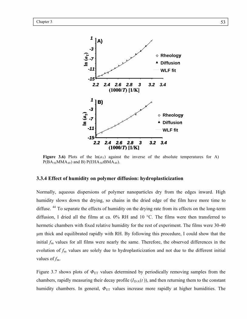
Chapter 3 53
(1000/T) [1/K]ln
(aT)
-15
-11
-7
-3
1
2.2 2.4 2.6 2.8 3 3.2 3.4
Rheology
Diffusion
WLF fit
A)
Rheology
Diffusion
WLF fit
-15
-11
-7
-3
1
2.2 2.4 2.6 2.8 3 3.2 3.4
ln(a
T)
(1000/T) [1/K]
B)
(1000/T) [1/K]ln
(aT)
-15
-11
-7
-3
1
2.2 2.4 2.6 2.8 3 3.2 3.4
Rheology
Diffusion
WLF fit
Rheology
Diffusion
WLF fit
A)
Rheology
Diffusion
WLF fit
-15
-11
-7
-3
1
2.2 2.4 2.6 2.8 3 3.2 3.4
ln(a
T)
(1000/T) [1/K]
B)
Rheology
Diffusion
WLF fit
Rheology
Diffusion
WLF fit
-15
-11
-7
-3
1
2.2 2.4 2.6 2.8 3 3.2 3.4
ln(a
T)
(1000/T) [1/K]
B)
Figure 3.6) Plots of the ln(aT) against the inverse of the absolute temperatures for A) P(BA50MMA49) and B) P(EHA50tBMA49).
3.3.4 Effect of humidity on polymer diffusion: hydroplasticization
Normally, aqueous dispersions of polymer nanoparticles dry from the edges inward. High
humidity slows down the drying, so chains in the dried edge of the film have more time to
diffuse. 44 To separate the effects of humidity on the drying rate from its effects on the long-term
diffusion, I dried all the films at ca. 0% RH and 10 °C. The films were then transferred to
hermetic chambers with fixed relative humidity for the rest of experiment. The films were 30-40
µm thick and equilibrated rapidly with RH. By following this procedure, I could show that the
initial fm values for all films were nearly the same. Therefore, the observed differences in the
evolution of fm values are solely due to hydroplasticization and not due to the different initial
values of fm.
Figure 3.7 shows plots of ΦET values determined by periodically removing samples from the
chambers, rapidly measuring their decay profile (ID/A(t’)), and then returning them to the constant
humidity chambers. In general, ΦET values increase more rapidly at higher humidities. The

Chapter 3 54
evolution of ΦET in P(BA50MMA49) strongly depends on humidity, whereas it shows less
sensitivity to humidity in P(EHA50tBMA49). Similar trends were revealed when fm values
(calculated by eq. 2.25, using simulated values of ΦET(0) and ΦET(∞) from Table 3.3) were
plotted against the aging time.
Time (min)
0
0.2
0.4
0.6
0 5000 10000 15000 20000
98%
23%
85%
54%
0%
RH:
ΦE
T
0
0.1
0.2
0.3
0.4
0 5000 10000 15000 20000
98%
23%
85%54%
0%
Time (min)
ΦE
T
RH:
A)
B)
Time (min)
0
0.2
0.4
0.6
0 5000 10000 15000 20000
98%
23%
85%
54%
0%
RH:
ΦE
T
Time (min)
0
0.2
0.4
0.6
0 5000 10000 15000 20000
98%
23%
85%
54%
0%
RH:
ΦE
T
0
0.1
0.2
0.3
0.4
0 5000 10000 15000 20000
98%
23%
85%54%
0%
Time (min)
ΦE
T
RH:
0
0.1
0.2
0.3
0.4
0 5000 10000 15000 20000
98%
23%
85%54%
0%
Time (min)
ΦE
T
RH:
A)
B)
Figure 3.7) Plots of the energy transfer efficiency ΦET vs. time for A) P(BA50MMA49) and B) P(EHA50tBMA49) at 0, 23, 54, 85 and 98% RH and 25 °C.
In Figure 3.8, Dapp values are plotted versus fm for P(BA50MMA49) and P(EHA50tBMA49). Here,
and also in Figure 3.3, Dapp values drop by nearly an order of magnitude as the fraction of
mixing increases. I attribute this to the contribution of slowly diffusing species such as high
molecular weight polymer or possibly branched chains that takes place at higher mixing
fractions. As fm approaches unity, energy transfer measurements loose their sensitivity to the
extent of diffusion.

Chapter 3 55
The diffusion coefficient values for P(BA50MMA49) are lower than those for P(EHA50tBMA49)
by nearly an order of magnitude. This is partly a reflection of the difference in molecular weight
of the samples. The acceptor labeled P(BA50MMA49) had Mw of 227,000 whereas Mw = 162,000
for the acceptor labeled P(EHA50tBMA49). If one ignores the difference in polymer composition,
one might imagine, based on the Reptation model (D~M-2), that this difference in molecular
weight might account for up to 2 times the difference in Dapp.
Another important parameter in Rouse and Reptation models is the monomeric friction
coefficient (ξ0). In homopolymers, ξ0 depends on the chemical structure of the repeating units in
a subtle way. Compared to other acrylates and methacrylates, PMMA has a very high ξ0 value
(log(ξ0,PMMA) = 0.66 at 398 °K). 45 ξ0 decreases significantly for polymers with bulky side
groups. 46 It is not trivial to calculate ξ0 for a random copolymer knowing ξ0 of its constituents.
A linear mixing rule was shown to provide good predictions for ξ0 of poly(styrene-b-isoprene),
whereas an Arrhenius mixing rule was proposed for poly(Sty-b-MMA). 45 47, I infer that
P(BA MMA ) has a higher average monomeric friction coefficient than P(EHA tBMA )
because of the presence of the bulky substitutes in the late
50 49 50 49
r copolymer.
Table 3.4. Vertical shift factors and equilibrium water content at different humidities.
RH% P( BA50MMA49)
Water wt% aH
P(EHA50tBMA49)
Water wt% aH
0 1 1
23 0.30 1.9 0.20 1.45
54 0.90 5.2 0.60 2.75
85 2.40 16.4 1.80 3.3
98 9.00 30.0 5.14 4.1

Chapter 3 56
0 0.2 0.6 0.8
98%
23%54%
0%M
0.4
RH:
85%
10-16
10-17
10-18
10-19
10-20
Dap
p(c
m2 /
s)
fm
B)
0 0.2 0.6 0.8
98%
23%85%
54%0%M
10-16
RH:
0.4
10-17
10-18
10-19
10-20
Dap
p(c
m2 /
s)
fm
A)
0 0.2 0.6 0.8
98%
23%54%
0%M
0.4
RH:
85%
10-16
10-17
10-18
10-19
10-20
Dap
p(c
m2 /
s)
fm
B)
0 0.2 0.6 0.8
98%
23%54%
0%M
0.4
RH:
85%
10-16
10-17
10-18
10-19
10-20
Dap
p(c
m2 /
s)
fm
0 0.2 0.6 0.8
98%
23%54%
0%M
0.4
RH:
85%
10-16
10-17
10-18
10-19
10-20
Dap
p(c
m2 /
s)
fm
B)
0 0.2 0.6 0.8
98%
23%85%
54%0%M
10-16
RH:
0.4
10-17
10-18
10-19
10-20
Dap
p(c
m2 /
s)
fm
A)
0 0.2 0.6 0.8
98%
23%85%
54%0%M
10-16
RH:
0.4
10-17
10-18
10-19
10-20
Dap
p(c
m2 /
s)
fm
A)
Figure 3.8) Plots of the apparent diffusion coefficient Dapp vs. aging time for A) P(BA50MMA49) and B) P(EHA50tBMA49) at 0, 23, 54, 85 and 98% RH and 25 °C, The master curves are shifted one unit down for clarity.
Analogous to how I studied the effect of temperature on diffusion, I built master curves by using
vertical shift factors (aH) that overlay the curves recorded at different relative humidity values
(RHs) on the one recorded at zero humidity. For both copolymers, the Dapp values associated
with the humidity master curve (at 0% RH and 25 °C) are at least two orders of magnitude lower
than those shown in Figure 3.3 with a reference temperature of 40 °C (and 0% RH). The detailed
shape of the master curve is primarily determined by the details of molecular weight distribution.
Therefore, for each copolymer, the shape of the master curves is similar regardless of the
reference temperature.

Chapter 3 57
The shift factors are a measure of the extent of hydroplasticization. The results show that water
absorbed by the film accelerates diffusion by a factor of 30 in P(BA50MMA49) whereas this
factor is only 4 for P(EHA50tBMA49). To make these data more comprehensible, I measured the
equilibrium water content gravimetrically. Table 3.4 shows the equilibrium water content along
with the aH values. At 85% relative humidity, P(BA50MMA49) picks up 2.4 wt% water whereas
P(EHA50tBMA49) peaks up 1.8 wt% water. I observed visually that both films became turbid at
98 % RH. This indicates the presence of phase separated regions of sufficient size to scatter
visible light.
To analyze these data quantitatively, I assume that moisture plasticizes the polymer by
decreasing the magnitude of the monomer friction coefficient (ζ0). For each sample, the polymer
diffusion rate depends upon the difference (T-Tg). Since the measurements were performed at a
constant temperature, the influence of moisture is to decrease Tg.
In the previous section, where the free volume increased as a consequence of increasing
temperature, I could use TTS to obtain temperature shift factors (aT). The WLF equation could
fit the aT values obtained at different ∆T. Similarly, it is possible to use aH values and obtain ∆T
from the WLF equation. Unlike measurements at different temperatures, in the humidity
experiments, the experimental temperature was constant and ∆T originated from a relative
decrease in samples Tg due to hydroplasticization.
.T2,
T2,T1,T1,
0T2,T2,
C
CCC
T),(TCC
00
0
(3.2)
By shifting the WLF parameter to the glass transition temperature (via eq 3.2) I estimated the
depression in the glass transition of P(BA MMA ) and P(EHA tBMA ) at 98% RH to be 8.5
and 4.5 °C, respectively. These values are comparable to what Sperry et al. reported for the
difference between wet and dry minimum film formation temperature.
50 49 50 49
Nawaz et al. reported a
20 °C drop in the glass transition for 50 nm PBMA particles which is indeed higher than what
can be explained by hydroplasticization alone.
It is important to note that this analysis is independent of the state of water in the film. However,
fundamentally the WLF parameters for the plasticized and the unplasticized system may not be

Chapter 3 58
the same. In other words, a plasticizer might specifically affect a given relaxation process besides
decreasing ζ0. It has been shown that moisture does not accelerate or retard a given relaxation
process in polymers.48 Having measured the WLF constants, I preferred to extend these
parameters to the plasticized state since predictive models for glass transition of hydroplasticized
samples do not provide a very accurate estimate.49
1/ln
(a H
)
0
1
2
3
0 100 200 300 400 500 600
P(EHA50tBMA49)
P(BA50MMA49)
φw-1
1/ln
(a H
)
0
1
2
3
0 100 200 300 400 500 600
P(EHA50tBMA49)
P(BA50MMA49)
φw-1
Figure 3.9) Plots of 1/ln(aH) vs. φw-1 based on the data in Table 3.4 For P(EHA50tBMA49) the intercept
and slope of the line are 0.530 and 0.004 respectively (R2 = 0.97). For P(BA50MMA49) the intercept and slope of the line are 0.205 and 0.004 respectively (R2 = 0.99).
If water acts as a traditional plasticizer and uniformly increases the free volume throughout the
sample, it should be possible to fit the data presented in Table 3.4 to the Fujita-Doolittle
equation. Fujita proposed a linear increase in the polymer free volume with the volume fraction
of added plasticizer (φ) (eq. 3.3).50 Here, (T) is the difference between the fractional free
volume of the polymer and that of the plasticizer at temperature T, and f(0, T) is the fractional
free volume of pure polymer; (T) is the factor by which the free volume increases, and its
magnitude is a measure of the plasticizer efficiency.
f(w,T) = f(0,T) + (T)w (3.3)
Fujita showed that combining eq. 3.3 with the Doolittle equation makes it possible to predict the
viscosity and the diffusion coefficient of a plasticized polymer (eq. 3.4). I attempted to fit the
data in Table 3.4 to the Fujita-Doolittle model. I assumed equal density for water and polymer so
that I could use wt % instead of vol. %.

Chapter 3 59
.)1
.()T(
)T,0(f)T,0(f
)aln(
1
))0,T(D),T(Dln(
1
w
2
Hw
(3.4)
Figure 3.9 illustrates these Fujita plots. As predicted by eq. 3.4, I obtained a linear relation
between 1/ln(aH) and 1/φw. However, the parameters obtained from these lines do not conform
to the theoretical expectations. These plots lead to values of ca. 10.5 for P(EHA50tBMA49) and
67 for P(BA50MMA49), respectively. These values are much higher than reported values for
other plasticizers; but more significantly, are contradictory to the definition that cannot be
greater than unity. In addition, the magnitude of the intercept does not match the value our group 51,52 and others obtained previously. The intercept of the Fujita fit is proportional to the free
volume of the pure polymer ( (0, )) at the experimental temperature. Following the WLF
approach, one can show that (0, ) 1/ , where is the first WLF parameter at the
f T
f T = C1 C1
experimental temperature.
ental data from the Fujita prediction is more prominent for films aged at
higher humidities.
At 25°C, the values of 1/C1 are 0.032 and 0.041 for P(EHA50tBMA49) and P(BA50MMA49)
respectively. If I fix the intercept at these values and attempt to fit the data to the Fujita equation,
the correlation coefficient (R2) decreases mildly for the hydrophilic P(BA50MMA49) but
significantly for the hydrophobic P(EHA50tBMA49), as shown in Figure 3.10. In addition, the
deviation of experim
0
1
2
3
0 200 400 600
P(BA50MMA49)
P(EHA50tBMA49)
1/ln
(a H
)
φW-1
0
1
2
3
0 200 400 600
P(BA50MMA49)
P(EHA50tBMA49)
1/ln
(a H
)
50 49) t 55 (R2 = 0.77). For P(BA50MMA49) the slope of the line is 0.0045 (R2 = 0.95).
φW-1
Figure 3.10) Plots of 1/ln(aH) vs. φw-1 where the intercept was fixed to the polymer free volume at
25° C. For P(EHA tBMA he slope of the line is 0.00

Chapter 3 60
3.3.5 FTIR analysis of water content in the films
In assessing the efficiency of water miscible plasticizers such as TexanolTM (2,2,4-trimethyl-1,3-
pentanediol monoisobutyrate, TPM), partitioning of the plasticizer plays a key role. 53 The
partition coefficient determines how plasticizer is partitioned between the water and the polymer
phase. Evidently, the fraction of plasticizer in the water phase does not contribute to the
plasticization process and should not be taken into account for calculating the parameter. In the
experiments described above, only water molecules that were molecularly dispersed among the
polymer chains could serve as plasticizer and increase the free volume. Water that resides in a
phase-separated state will not contribute in this way.
0
0.05
0.1
0.15
0.2
0.25
3050 3250 3450 3650 3850
Wavenumber (cm-1)
B) P(EHA50tBMA49) 98%
85%
23%54%
3050 3250 3450 3650 3850
0.25
0.2
0.15
0.1
0.05
0
Abs
orba
nce
(a.u
.)
0
0.05
0.1
0.15
0.2
0.25
3050 3250 3450 3650 3850
A) P(BA50MMA49) 98%
85%
54%23%
3050 3250 3450 3650 3850
0.25
0.2
0.15
0.1
0.05
0
Ab
sorb
ance
(a.
u.)
Wavenumber (cm-1)
0
0.05
0.1
0.15
0.2
0.25
3050 3250 3450 3650 3850
Wavenumber (cm-1)
B) P(EHA50tBMA49) 98%
85%
23%54%
3050 3250 3450 3650 3850
0.25
0.2
0.15
0.1
0.05
0
Abs
orba
nce
(a.u
.)
0
0.05
0.1
0.15
0.2
0.25
3050 3250 3450 3650 3850
Wavenumber (cm-1)
B) P(EHA50tBMA49) 98%
85%
23%54%
3050 3250 3450 3650 3850
0.25
0.2
0.15
0.1
0.05
0
Abs
orba
nce
(a.u
.)
0
0.05
0.1
0.15
0.2
0.25
3050 3250 3450 3650 3850
A) P(BA50MMA49) 98%
85%
54%23%
3050 3250 3450 3650 3850
0.25
0.2
0.15
0.1
0.05
0
Ab
sorb
ance
(a.
u.)
Wavenumber (cm-1)
0
0.05
0.1
0.15
0.2
0.25
3050 3250 3450 3650 3850
A) P(BA50MMA49) 98%
85%
54%23%
3050 3250 3450 3650 3850
0.25
0.2
0.15
0.1
0.05
0
Ab
sorb
ance
(a.
u.)
Wavenumber (cm-1)
Figure 3.11) FTIR spectra (in the OH stretching region) of water absorbed into the copolymer films at different relative humidities
Phase separation of absorbed water in polymers has been reported for many polymers and resins. 17- ,19 23 The important question that arises is at which point water starts to phase separate from the

Chapter 3 61
film. Figure 3.11 shows FTIR spectra in the νOH stretching region for both copolymers. The
major feature of the spectra is that the intensity of the broad unresolved νOH band (in the region
3050 to 3700 cm -1) increases at higher humidities.
Table 3.5. Spectroscopic parameters of water absorbed to P(BA50MMA49) at different water activities in the film (relative humidity)
aw Position ± 2 (cm-1) Intensity fwhm(cm-1) Relative area(%)
0.98
3280
3445
3561
3636
0.112
0.148
0.124
0.061
308
185
126
66
46.5
32.1
17.0
4.4
0.85
3280
3445
3561
3636
0.040
0.053
0.066
0.037
320
179
127
65
38.7
28.7
25.3
7.3
0.54
3280
3445
3561
3636
--
0.020
0.030
0.017
--
133
114
55
--
37.5
49.0
13.5
0.23
3280
3445
3561
3636
--
0.007
0.019
0.014
--
108
110
58
--
20
57.5
22.5

Chapter 3 62
The unresolved νOH interval corresponds to the different states of water that are present in the
film i.e hydrogen bonded water, water monomers, dimers and free water. ,19 16 The reason for the
appearance of several bands is that the time scale of vibration is much shorter than the time scale
of hydrogen bond formation. To resolve the νOH multicomponent band I used a curve-fitting
algorithm based on the Levenberg-Marquardt minimization method. In all cases, I used mixed
Gaussian-Lorentzian peaks.54 For each copolymer, the baseline, band shape and the number of
components were fixed and the minimization algorithm was allowed to find the height, position,
and full width at half maximum (fwhm) of each peak.
0
0.05
0.1
0.15
0.2
0.25
3050 3250 3450 3650 3850
Wavenumber (cm-1)
Abs
orba
nce
(a.
u.)
0
0.05
0.1
0.15
0.2
0.25
3050 3250 3450 3650 3850
Wavenumber (cm-1)
Abs
orba
nce
(a.
u.)
0
0.05
0.1
0.15
0.2
0.25
3050 3250 3450 3650 3850
Wavenumber (cm-1)
Abs
orba
nce
(a.u
.)
0
0.05
0.1
0.15
0.2
0.25
3050 3250 3450 3650 3850
Wavenumber (cm-1)
Abs
orba
nce
(a.u
.)
A)
B)
0
0.05
0.1
0.15
0.2
0.25
3050 3250 3450 3650 3850
Wavenumber (cm-1)
Abs
orba
nce
(a.
u.)
0
0.05
0.1
0.15
0.2
0.25
3050 3250 3450 3650 3850
Wavenumber (cm-1)
Abs
orba
nce
(a.
u.)
0
0.05
0.1
0.15
0.2
0.25
3050 3250 3450 3650 3850
Wavenumber (cm-1)
Abs
orba
nce
(a.u
.)
0
0.05
0.1
0.15
0.2
0.25
3050 3250 3450 3650 3850
Wavenumber (cm-1)
Abs
orba
nce
(a.u
.)
A)
B)
Figure 3.12) Curve-fitting analysis results of isolated FTIR spectra obtained on films aged at 98% RH. A) P(BA50MMA49) and B). P(EHA50tBMA49)
To reduce the number of fitting parameters, I used the minimum number of bands that would
afford a good fit to the experimental spectra. For P(BA50MMA49), at least four bands were
needed to resolve the peak with good fitting quality (judged by minimizing χ2). Figure 3.12A
represents an example of resolved bands for the P(BA50MMA49) film at 98% relative humidity.

Chapter 3 63
In the case of P(EHA50tBMA49), using two bands results in an accurate representation of the
FTIR spectra. Figure 3.12B shows the curve-fitting analysis results for P(EHA50tBMA49) at 98%
relative humidity. P(EHA50tBMA49) absorbed ca. 0.2 wt% water at 23% RH. The isolated FTIR
spectrum of this sample was noisy with weak intensity. Therefore, I could not resolve the peaks
meaningfully by the curve fitting approach.
In Table 3.5 and 3.6 I present results of band fitting for both copolymers at different water
activities. There is some controversy in the literature about assigning the band corresponding to
free water. Cotugno et al. assigned the resolved peak that appeared at the highest frequency
(3629 cm-1) to unassociated water in an epoxy resin matrix. Sutandar et al., in analyzing the state
of water absorbed in poly(methyl methacrylate) films, assigned the peak that appeared at the
lowest frequency (3382 cm-1) to free water in the film.
Table 3.6. Spectroscopic parameters of water absorbed to P(EHA50tBMA49) at different water activities in the film (relative humidity). At aw=0.23 the analysis was not possible due to very low water content.
aw Position ± 2 (cm-1) Intensity fwhm(cm-1) Relative area(%)
0.98
3336
3515
0.142
0.104
365
243
66.2
33.8
0.85
3336
3515
0.030
0.040
438
237
58.8
41.2
0.54
3336
3515
--
0.009
--
201
--
100
Table 3.5 and 3.6 show that at lower relative humidities, the lower frequency peak (at 3280 cm-1
for P(BA50MMA49) and at 3336 cm-1 for P(EHA50tBMA49)) disappears. Therefore, I assigned
the low frequency peaks to unassociated water that does not contribute to the plasticization
process. The results show that at 23 and 54% RH, there is no detectable free water in the sample.

Chapter 3 64
With the notion that at 23 and 54% RH almost all of the absorbed water participates in
accelerating diffusion, I reconstruct the Fujita plots in Figure 3.13. Here I fixed the intercept of
the plot to the free volume of the polymer at 25°C. I present, for comparison, the points
corresponding to 85 and 98% RH on the same plot. As illustrated by the shaded envelop, at low
values of (φw)-1, phase-separated water is more significant for P(EHA50tBMA49). Based on this
analysis, I calculated the β value to be 0.36 for P(BA50MMA49) and 0.19 for P(EHA50tBMA49).
These values are significantly larger than what has been reported for common plasticizers such
as TPM (with β ~ 0.07). More importantly, they lay within the theoretical expectation of Fujita-
Doolittle model. The values of β obtained for water in this study are comparable to values
reported by Fujita and Kishimoto.55 For water as diluent, they reported a value of 0.37 in
poly(vinyl acetate) and a value of 0.3 in poly(methyl acrylate).
A)P(BA50MMA49)
B)P(EHA50tBMA49)
A)P(BA50MMA49)
B)P(EHA50tBMA49)
Figure 3.13) Reconstructed Fujita plots based on the dual nature of water. The dashed area represents the phase-separated water in the films.

Chapter 3 65
3.4 Summary
I examined the influence of humidity on the diffusion rate for copolymers of BA/MMA and
EHA/tBMA. These copolymers were designed to have similar glass transition temperature but
different hydrophilicity. By studying diffusion rate at different temperatures, I obtained TTS shift
factors that correlate with those obtained from the bulk polymer by rheology measurements. In
addition, the shift factors comply with a linear increase of the free volume with temperature and
can be fitted with the WLF equation. The WLF constants provided us with the important
parameter 1/C1 at 25 °C, which corresponds to the fractional free volume of each copolymer at
25 °C.
To analyze polymer diffusion rate at different relative humidities, I used a master curve analysis
based upon humidity-related shift factors. I showed that these raw shift factors do not comply
with the assumption of a linear increase in the free volume with the mass (volume) fraction of
water absorbed by the sample. Based on the observation of turbidity of the films and FTIR
measurements, I confirmed the presence of free water in the films at high humidities. This
fraction of water does not contribute to plasticization. To compare the efficiency of water in
promoting diffusion rate, I analyzed the data in the framework of the Fujita-Doolittle model.
Meaningful β parameters were obtained only after the presence of free water in the film was
properly taken into account. The results showed that molecularly dispersed water is much more
efficient in promoting diffusion in latex films than other well-known plasticizers.
I envision two mechanisms by which water promotes polymer diffusion rates in these polymer
films. First, water contributes to the free volume of the film as a consequence of its low glass
transition temperature. Water shows weak glass forming signatures,56 and thus it is challenging
to measure accurately its glass transition temperature. Values between 120 to 160 K have been
reported in the literature. The most widely adopted value is 136 K.57 Thus, water is
characterized by a much lower Tg than conventional plasticizers. Hence, even at very low
volume fractions, water molecules can contribute significantly to the free volume of the system
and cause extensive plasticization at room temperature.
The second mechanism is associated with the presence of –COOH groups in the latex polymer.
In the absence of water, the presence of –COOH groups slows down the rate of polymer
diffusion,58 presumably because of hydrogen bonding between the acidic –OH and the ester
Chapter 3 66
carbonyl groups of the polymer molecules. One can imagine that in films containing water, the
water molecules can compete with the carboxylic acid groups in the latex polymer in forming
hydrogen bonds with these ester C=O groups. In this way, water can lubricate the diffusion
process. At this point, it is not clear which mechanism is dominant. Performing the same
experiments with dispersions synthesized without any MAA added may be helpful in this regard.
The reviewer of the thesis pointed out that the value of β obtained for TPM in latex polymers
may be influenced by hydroplasticization. To obtain the β value for TPM for a given polymer,
one adds various amount of this compound to a latex dispersion and then casts and dries a film.
Then one uses FRET experiments to monitor polymer diffusion, following a path similar to what
was described in this chapter, i.e. obtaining shift factors by vertically shifting Dapp vs fm curves
recorded for films containing TPM and overlaying them on the Dapp vs fm curve recorded for the
TPM free film. 59,60 The shift factors obtained in this way can be fitted to the Fujita-Doolittle
model to obtain β. The reviewer argued that these experiments were performed at a certain RH.
In fact, the β value I reported for TPM was obtained from experiments that were performed at
54% RH. However, I believe that hydroplasticization does not have a noticeable effect on this
value.
TPM is a fairly hydrophobic compound. Partitioning coefficient measurements showed that
when TPM is added to a latex dispersion, its concentration in the polymer phase is about 400
times higher than the concentration in the aqueous phase. Given the hydrophobic nature of TPM,
water uptake of the film is not expected to change significantly upon addition of this compound.
Hence, the extent of hydroplasticization is the same is all samples regardless of their TPM
content. In this way, the vertical shift factors obtained at 54% RH for films containing various
amount of TPM should depend solely on the TPM content of the films and not on the ambient
humidity. I expect that one would obtain the same value β = 0.07±0.01 for P(BA-MMA) or
P(EHA-tBMA) if the measurements were done at 0% RH.
Chapter 3 67
3.5 References
1 Struik, L. C. E. Physical Aging in Amorphous Polymers and Other Materials; Elsevier:
Amsterdam, 1978.
2 Bley, O.; Siepmann, J.; Bodmeier, R. J. Pharm. Sci. 2009, 98, 651-664.
3 Chang, R. K.; Raghavan, K. S.; Hussain, M. A. J. Pharm. Sci. 1998, 87, 556–558.
4 Kuentz, M.; Röthlisberger, D. Int. J. Pharm. 2002, 236, 145-152.
5 Cole, E. T.; Cadé, D.; Benameur, H. Adv. Drug Delivery Rev., 2008, 60, 747-756.
6 Kinloch, A. J.; Korenberg, C. F., Tan, K. T.; Watts, J. F.; J. Mater. Sci. 2007, 42, 6353-6370.
7 Tan, K. T.; Vogt, B. D.; White, C. C.; Steffens, K. L.; Goldman, J.; Satija, S. K.; Cleric, C.;
Hunston, D. L. Langmuir 2008, 24, 9189-9193.
8 Jubete, E.; Liauw, M.; Allen, N. Prog. Org. Coat. 2007, 59, 126-133.
9 Mijovic, J.; Lin, K.; J. Appl. Polym. Sci. 1985, 30, 2527.
10 Banks, L.; Ellis, B. Polym. Bull. 1979, I, 377.
11 Brinke, G., Karasz, F. E.; Ellis, T. S. Macromolecules 1983, 16, 244-249.
12 Jelinski, L. W.; Dumais, J. J.; Cholli, A. L. ; Ellis, T. S. ; Karasz Macromolecules 1985, 18,
1091-1095.
13 Ellis, T. S.; Karasz, F. E. Polymer 1984, 25, 664-669.
14 Couchmann, P. R.; Karasz, F. E.; Macromolecules 1978, 11, 117-119.
15 Dias, C. R.; Rosa, M. J.; Pinho, M. N. J. Memberane Sci. 1998, 259-267.
16 Sutandar, P.; June Ahn, D.; Franses, E. I. Macromolecules 1994, 27, 7316-7328.
Chapter 3 68
17 Hodge, R. M. Polymer 1996, 37, 1371-1376.
18 Hodge, R. M.; Bastow, T. J.; Edward, G. H.; Simon, G. P.; Hill, A. J. Macromolecules 1996,
29, 8137-8143.
19 a) Musto, P.; Ragosta, G.; Mascia, L. Chem. Mater. 2000, 12, 1331-1341. b) Cotugno, S.;
Mensitieri, G.; Musto, P.; Sanguigno, L. Macromoleculs 2005, 35, 801-811.
20 Zhou, J.; Lucas, J. Polymer 1999, 5505-5512.
21 Wang, B.; Gong, W.; Liu, W. H.; Wang, Z. F.; Qi, N.; Li, X. W.; Liu, M. J.; Li, S. J. Polymer
2003, 44, 4047-4052.
22 Soles, C.; Chang, F. T.; Gidley, D. W.; Yee, A. F. J. Polym. Sci., Part B: Polym. Phys. 2000,
38, 776-791.
23 a) Mijovic, J.; Zhang, H. Macromolecules 2003, 36, 1279. b) Zhang, H.; Mijovic, J.
Macromolecules 2004, 37, 5844-5846.
24 Sperry, P. R.; Snyder, B. S.; O’Dowd, M. L.; Lesko, P. M. Langmuir 1994, 10, 2619-2628.
25 Lin, F.; Meier, D. J. Langmuir 1996, 12, 2774-2780.
26 Lin, F.; Meier, D. J. Langmuir 1995, 11, 2726-2733.
27 Rottstegge, J.; Traub, B.; Wilhelm, M.; Landfester, K.; Heldmann, C.; Spiess, W. Macromol.
Chem. Phys. 2003, 204, 787–802.
28 Veniaminov, A.; Eckert, T.; Sillescu, H.; Bartsch, E. Macromolecules 2003, 36 , 4944-4953.
29 Veniaminov, A.; Jahr T.; Sillescu, H.; Bartsch E. Macromolecules 2002, 35, 808-819.
30 Nawaz, Q.; Rharbi, Y. Macromolecules 2008, 41, 5928-5933.
31 Turshatov, A.; Adams, J.; Johannsmann, D. Macromolecules 2008, 41, 5365-5372.

Chapter 3 69
32 Oh, J. K.; Wu, J.; Winnik, M. A.; Craun, G. P.; Rademacher, J.; Farwaha, R. J. Polym. Sci. A
Polym. Chem. 2002, 40, 3001-3011.
33 Sosnowski, S.; Feng, J.; Winnik, M. A. J. Polym. Sci. Part A: Polym. Chem. 1994, 32, 1497-
1505.
34 Tronc, H.; Liu, R.; Winnik, M. A.; Eckersley, S. T.; Rose, G. D.; Weichuhn, J. M.; Meunier,
D. M. J. Polym. Sci. Part A: Polym. Chem. 2002, 40, 2609-2625.
35 Pathak, J. A.; Colby, R. H.; Kamath, A. Y.; Kumar, S. K.; Stadler, R. Macromolecules 1998,
31, 8988.
36 Koenig, J. L. Spectroscopy of Polymers; American Chemical Society, Washington, DC, 1992.
37 James, D. R.; Demmer, D. R. M.; Verrall, R. E.; Steer, R. P. Rev. Sci. Instrum. 1983, 54,
1121–1130.
38 Greenspan, L. J. Res. NBS A Phys. Chem. 1977, 81A, 89.
39 Wu, J.; Tomba, J. P.; Winnik, M. A.; Farwaha, R.; Radmacher, J. Macromolecules 2004, 37,
2299.
40 Oh, J. K.; Yang, J.; Tomba, J. P.; Winnik, M. A.; Farwaha, R.; Radmacher, J. Macromoleculs
2003, 36, 8836.
41 Liu, Y.; Haley, J. C.; Deng, K.; Lau, W.; Winnik, M. A. Macromolecules 2007, 40, 6422-
6431.
42 Farinha, J. P. S.; Vorobyova, O.; Winnik, M. A.; Macromoleculs 2000, 33, 5863-5873.
43 Ferry, J. D. Viscoelastic Properties of Polymers; Wiley: New York, 1980.
44 Haley, J. C.; Liu, Y.; Winnik, M. A.; Lau, W. J. Coat. Technol. Res. 2008, 5, 157-168.
45 Milhaupt, J. M.; Lodge, T. P.; Smith, S. D.; Hamersky, M. W. Macromolecules 2001, 34,
5561-5570.
Chapter 3 70
46 Kurath, S. F.; Yin, T. P.; Berge, J. W.; Ferry, J. D. J. Colloid Sci. 1959, 14, 147-160.
47 Chapman, B. R.; Hamersky, M. W.; Milhaupt, J. M.; Kostelecky, C.; Lodge, T. P.; von
Meerwall, E. D.; Smith, S. D. Macromolecules 1998, 31, 4562-4573.
48 a) Yildiz, M. E.; Kokini, J. L. J. Rheol. 2001, 45, 903-912. b) Ogawa, T.; Inoue, A.; Osawa, S.
J. Appl. Polym. Sci. 1998, 69, 315-321.
49 Hancock, B.; Zografi, G. Pharm. Res. 1994, 11, 471- 477.
50 Fujita, H. Fortschr. Hochpolym.-Forsch. 1961, 3, 1.
51 Odrobina, E.; Feng, J.; Winnik, M. A. J. Polym. Sci. Part A: Polymer Chemistry 2000, 38,
3933.
52 Juhué, D.; Wang, Y.; Winnik, M. A. Makromol. Chem. Rapid Commun. 1995, 16, 861.
53 Schroeder, W. F.; Liu, Y.; Tomba, J. P.; Soleimani, M.; Lau, W.; Winnik, M. A. J. Phys.
Chem. B 2010, 114, 3085-3094.
54 Maddams, W. F.; Appl. Spectrosc. 1980, 34, 245.
55 Fujita, H.; Kishimoto, A. J Polym Sci, 28 (1958), pp. 547–567
56 Angell, C. A. Science 2008, 319, 582-587.
57 Johari, G. P. J. Chem. Phys. 2003, 119, 2935-2937.
58 Kim, H.-B.; Wang, Y.; Winnik, M.A. Polymer 1994, 35, 1779-1786.
59 Schroeder, W. F.; Liu, Y.; Tomba, J. P.; Soleimani, M.; Lau, W.; Winnik, M. A. J. Phys.
Chem. B 2010, 114, 3085-3094.
60 Liu, Y.; Schroeder, W.; Soleimani, M.; Lau, W.; Winnik, M. A. Macromolecules 2010, 43,
6438-6449.

Appendix 1 71
Appendix 1
Transmission FTIR spectra for films of P(BA MMA ) and P(EHA tBMA ) aged
at different relative
50 49 50 49
humidities.
-0.1
0.5
1.1
1.7
26002800300032003400360038004000
-0.1
0.5
1.1
1.7
98%85%
54%
23%0%
Wavenumber (cm-1)
Abs
orba
nce
(a.u
.)
A) P(BA50MMA49)
-0.1
0.5
1.1
1.7
26002800300032003400360038004000
-0.1
0.5
1.1
1.7
98%85%
54%
23%0%
Wavenumber (cm-1)
Abs
orba
nce
(a.u
.)
-0.1
0.5
1.1
1.7
26002800300032003400360038004000
-0.1
0.5
1.1
1.7
98%85%
54%
23%0%
98%85%
54%
23%0%
98%85%
54%
23%0%
Wavenumber (cm-1)
Abs
orba
nce
(a.u
.)
A) P(BA50MMA49)
-0.1
0.5
1.1
1.7
26002800300032003400360038004000
-0.1
0.5
1.1
1.7
Wavenumber (cm-1)
Ab
sorb
ance
(a.
u.)
98%85%54%23%0%
B) P(EHA50tBMA49)
-0.1
0.5
1.1
1.7
26002800300032003400360038004000
-0.1
0.5
1.1
1.7
Wavenumber (cm-1)
Ab
sorb
ance
(a.
u.)
98%85%54%23%0%
-0.1
0.5
1.1
1.7
26002800300032003400360038004000
-0.1
0.5
1.1
1.7
Wavenumber (cm-1)
Ab
sorb
ance
(a.
u.)
98%85%54%23%0%
98%85%54%23%0%
98%85%54%23%0%
B) P(EHA50tBMA49)
Figure A1.1) Transmission FTIR spectra for films of A) P(BA50MMA49) and B) P(EHA50tBMA49) aged at different relative humidities.

Chapter 4 72
CHAPTER FOUR
Effect of molecular weight distribution on polymer diffusion rate
during film formation of two-component high-/low-molecular
weight latex particles i
4.1 Introduction
Multicomponent polymer nanoparticles are technologically important in the fabrication of high
performance and commodity materials such as water borne coatings, printing inks, caulks,
varnishes and pressure sensitive adhesives.1 Strictly speaking, two-component materials provide
cost effective routes to new properties without the requirement for synthesizing totally new
molecules. Miscible polymer blends represent a small class of multicomponent polymer
materials. These blends are homogenous on length scales at which immiscible blends
demonstrate composition heterogeneity. However, on much smaller length scales, miscible
blends exhibit dynamic heterogeneity that can result in useful properties such as broadness of
segmental relaxation times and glass transition.2 I use the term “two-component” nanoparticles
to describe polymer (latex) nanoparticles consisting of two polymers of essentially the same
composition that differ substantially in their molecular weight (M). This strategy enabled me to
engineer the molecular weight distribution (MWD) of these materials. I use the term two-
component polymers to describe polymer samples obtained by freeze-drying dispersions of the
two-component latex nanoparticles.
In the coatings formulation, many additives are added to dispersions of polymer particles to
lower the glass transition temperature (Tg) of the polymer. These additives commonly lead to
latex films with reduced mechanical strength that are tacky to the touch (too soft), have poor
tensile strength, and can creep once applied to a substrate. Blends of high- and low- molecular
i This chapter appeared as: “Effect of molecular weight distribution on polymer diffusion during film formation of two-component high-/low-molecular weight latex particles” Soleimani, M.; Khan, S.; Mendenhall, D.; Lau, W.; Winnik, M. A. Polymer 2012.

Chapter 4 73
weight (high-M, low-M) polymers allow one to avoid many of these problems. These blends take
advantage of the fact that the addition of small amounts of a low-M polymer to a high-M
polymer matrix has a significant effect on the number average molecular weight (Mn) of the
blend, but a much smaller, and sometimes negligible effect on the weight average molecular
weight (Mw). Some desirable properties of latex polymers, such as the free volume, which affects
Tg and the rate of polymer diffusion in latex films, depends upon Mn. On the other hand, many
mechanical and rheological properties, such as the polymer zero-shear viscosity and fracture
toughness, depend upon Mw.
Films made from a high Tg polymer are mechanical strong. However, particles made from these
polymers are not soft enough to deform under forces generated by water evaporation. Moreover,
these polymers are glassy at room temperature and thus exhibit very slow diffusion rates. On the
other hand, although soft polymer particles are film forming, they turn into tacky films with poor
mechanical properties.
Traditionally the challenge of achieving hard films from soft polymer particles was surmounted
by adding volatile organic plasticizers (VOCs) to a dispersion of high Tg latex particles. These
additives lower the Tg and thereby soften the particles, ease film formation and enhance the rate
of polymer diffusion across particle boundaries. Therefore, they serve as both coalescing aids
and diffusion promoters. Then, they evaporate slowly to the atmosphere. Following the loss of
these additives, the Tg of the polymer increases and the mechanical properties improve. The
unwelcome aspect of this strategy is that VOCs are air pollutants and contribute to ground level
ozone formation and global warming. Regulatory agencies demand further decreases of VOC
emissions from coatings due to adverse health and environmental effects. Therefore, new
knowledge is needed to tune the mechanical properties of particles and final coatings without
adding VOCs. In this chapter, I introduce controlled broadening of MWD as a strategy for
modifying the film formation behavior of latex dispersions. This idea was developed during my
discussions with Dr. Willie Lau, our industrial collaborator. I based my design on the fact that
specific properties of polymers depend upon particular moments of the molecular weight
distribution.
The glass transition temperature (Tg) is the most important single parameter that determines bulk
mechanical properties of an amorphous polymer at a given temperature. According to free-

Chapter 4 74
volume theory, the glass transition is an iso-free volume state. Terminal units contribute more to
the free-volume than the backbone repeat units. Therefore, Tg scales inversely with the number
average molecular weight of a polymer as captured by Kanig-Ueberreiter equation: 3
1/Tg(Mn) = 1/Tg(∞) + K/Mn (4.1)
where K is a constant and Tg(∞) is the glass transition temperature at infinite molecular weight.
Polymer diffusion rates are coupled to the free volume through the magnitude of the monomeric
friction coefficient ξ. 4 Free-volume theory predicts that increasing temperature and addition of
plasticizers decreases ξ. Our group showed that the effect of temperature, Tg, and plasticizers on
polymer diffusion rates in latex films can be described by free-volume theory.5,6
For an entangled amorphous polymer above (Tg), the zero shear rate viscosity (η0) scales with
weight average molecular weight as:
η0 α Mw3.4-3.6 for Mw>Mc (4.2)
where the critical molecular weight (Mc) is typically 2-4 times larger than the entanglement
molecular weight (Me).7 Graessley predicted an even stronger dependence of η0 on the high
molecular mass component and predicted that η0 is a function of MwMzMz+1, , where Mz and
Mz+1 refer to the third (z-average MW) and fourth moment of the molecular weight
distribution..8 Equation 4.2 was originally obtained for monodisperse polymers. Studies on
polydisperse polyisobutylene and polyethylene showed that eq 4.2 holds for samples with
polydispersity in molecular weight as well.9 For bi- and trimodal blends of polystyrene it was
shown that η0 follows the same trend with Mw as samples with low polydispersity index (PDI). 10
Most water-borne dispersions are synthesized by free radical emulsion polymerization. During
this process, the average molecular weight can be varied by changing the type of initiator,
adjusting its concentration or using a chain transfer agent (CTA). However, polymers
synthesized in this way have a modest molecular weight distribution with a Mw/Mn of ca. 2.
Some years ago, our group noticed the signature of a low molecular weight fraction in the gel
permeation chromatography (GPC) trace of poly(butyl methacrylate) dispersion polymers
prepared by seeded emulsion polymerization. 11 This fraction was mostly water soluble and
could be separated by sedimentation of the polymer particles via high speed centrifugation. It
was shown that this low-M additive, post added to the latex particles, could increase the polymer
diffusion rate in latex films.

Chapter 4 75
A more convenient way of using low-M polymeric additives as diffusion promoters in latex films
is through latex blending.12 In this approach, a low-M dispersion is synthesized with a recipe rich
in an appropriate chain transfer agent. Then a suitable amount of particles consisting of low-M
polymer is blended with the film forming (high-M) dispersion. The two components are designed
to be miscible but differ in the concentrations of the end groups. After coalescence, the low-M
molecules must diffuse into the cells containing high-M polymers. This process should take
place over a relatively short time scale so the film can homogenize quickly after drying. The
homogenization time depends on the amount and molecular weight of the oligomeric latex, the
Tg of the high- and low-M particles and miscibility of the two components.
The approach described above requires blending very soft particles consisting of a low-M
polymer with considerably harder particles consisting of high-M molecules. These particles may
also vary in size and size distribution. Tzitzinou et al. showed that when large soft particles were
blended with small hard particles, air voids appeared in the final film even when the weight
fraction of hard particles was as low as 20%.13 Therefore, even at such low weight fractions,
hard particles segregated and formed non-film forming occlusions. On the other hand, large hard
particles formed clusters and created large air voids even when blended with up to 45 wt% of
small soft particles. The presence of non-film forming occlusions and air voids has many
deleterious effects on final film properties and leads to poor gloss in coatings.
Multicomponent particles represent an alternative approach to avoid problems originating from
the difference in modulus of nanoparticles in a latex blend. Recently, scientists at Dow reported
the use of in situ emulsion polymerization to prepare two-component particles that are amenable
to latex blending. 14 These two-component particles consisted of a high-M hard polymer that was
softened by the addition of a low-Tg oligomer. These particles were then blended with soft-one-
component particles, designed to have the same modulus as the two-component particles. Fasano
et al. showed that latex films from this blend were smooth and had high gloss. In contrast, films
prepared from blends of the soft-one-component particles and unmodified hard-particles (with a
significant difference in modulus) showed poor gloss. What was particularly special about their
experimental design is that the composition of the oligomer was tuned to be more miscible with
the soft polymer of the one-component particles. Thus, after coalescence the low-M polymer
migrated from the two-component particles into the soft polymer. Fasano et al. observed
percolation of oligomer-modified particles whereas unmodified hard particles agglomerated in

Chapter 4 76
the film and formed non-film-forming occlusions. Thus, in a blend containing oligomer-modified
hard particles, the two-component particles percolate and eventually regain hardness after
coalescence, leading to improved mechanical properties in the film, without loss of gloss. This
combination of properties is difficult to achieve by traditional latex blending.
In this study, I explore the role of oligomers incorporated by in situ emulsion polymerization as
diffusion promoters in latex films. I synthesized two-component latex particles following the
strategy described in Ref 14, using a high molecular weight dye-labeled latex particle as the seed
latex and generating (unlabeled) oligomer in situ in the second stage emulsion polymerization
(Scheme 4.1). To ensure miscibility and to be able to carry out an in-depth analysis of the
polymer diffusion data, I studied oligomers which had the same composition as the high-M
polymer. Polymer diffusion rates at room temperature were followed by fluorescence resonance
energy transfer (FRET) measurements. I studied diffusion rates in latex films prepared from
samples containing different amounts of oligomers, as well as samples to which oligomers with
different molecular weights were incorporated. I performed similar measurements on latex films
prepared by blending high-M latex with oligomer latex. I compared the consequence of the
incorporation strategy (blending versus sequential emulsion polymerization) on the efficiency of
oligomers as plasticizers Finally, the efficiency of oligomers as diffusion promoters was
compared with that of 2,2,4-trimethyl-1,3-pentanediol monoisobutyrate (Texanol™, TPM), a
traditional coalescing aid.
PMMA-seed (40 nm) A
AA
A
A-P(BA50MMA49)
1st seeded emulsion
polymerization
2nd seeded emulsion
polymerization
A-P(BA50MMA49) + Oligomer
A A
AA
PMMA-seed (40 nm) A
AA
A
AA
AA
A-P(BA50MMA49)
1st seeded emulsion
polymerization
2nd seeded emulsion
polymerization
A-P(BA50MMA49) + Oligomer
A A
AA
A A
AA
Scheme 4.1) Synthesis strategy used for the preparation of two-component nanoparticles containing acceptor-labeled P(BA50MMA49) and a fraction of a non-labeled oligomer.

Chapter 4 77
4.2 Experimental
4.2.1 Materials
Potassium persulfate (KPS), sodium bicarbonate (NaHCO3), 1-dodecanethiol (C12-SH) and
sodium dodecyl sulfate (SDS) were purchased from Aldrich and used as received. Methyl-β-
cyclodextrin (Me-β-CD) (Wacker Chemie) was used as a phase transfer catalyst. Methyl
methacrylate (MMA), butyl acrylate (BA) were purified from hydroquinone inhibitors by
passing through an inhibitor remover column (Aldrich). Methacrylic acid (MAA) was purchased
from Aldrich and used as received. Phenanthrylmethyl methacrylate (PheMMA) was purchased
from Toronto Research Chemicals Inc. and used without further purification. Dimethylamino-2-
methacryloxy-5-methylbenzophenone (NBenMA) was synthesized and used as acceptor dye.
Water was purified by a Milli-Q ion exchange filtration system.
4.2.2 Synthesis of Dimethylamino-2-methacryloxy-5-methylbenzophenone. (NBen-
MA) ii
A new strategy for synthesizing NBen-MA was developed by Dr. David Mendenhall, Eastern
Sources Inc.. A mixture of p-dimethylaminobenzoic acid (3.00g, 0.0182mol) and 20 mL
dichloromethane (DCM) was cooled to -25 °C and treated with 2.75g (0.023 mol) thionyl
chloride in one portion with vigorous swirling. Thionyl chloride should be handled with care as it
is a reactive compound that can explosively release dangerous gases upon contact with water and
other reagents. It is corrosive; causes burns to any area of contact; its vapor causes severe
irritation to skin, eye and respiratory system. After standing at 0 °C for 1.5h, the mixture was
filtered and concentrated on a rotary evaporator (bath 50 °C). The mixture was dissolved in
additional portions of DCM and reconcentrated by rotary evaporator until a dry white solid was
obtained. To the flask was added 20 mL DCM and 2.46g (0.0201 mol) p-methylanisole, and the
mixture was cooled to -25 °C. With magnetic stirring, 7.28g (0.0546 mol) anhydrous aluminum
chloride was added in portions,15 and the red solution was then stirred overnight with provisions
to trap the evolved HCl. The DCM was partially evaporated (rotary evaporator) and the solution
was stirred at room temperature for 10 hours. The solution was then poured into 50 mL
ii This synthesis was performed by Dr. David Mendenhall at Eastern Sources Inc. Elmsford, NY 10523.

Chapter 4 78
magnetically-stirred water containing a small amount of HCl. The reaction flask was rinsed with
50 mL DCM and added to the mixture. After the alumina had dissolved, the organic layer was
washed successively with water, 1% sodium bicarbonate, and water. Concentration on the rotary
evaporator gave 4.0 g green oil. Addition of 4 g 95% ethanol caused immediate crystallization of
2-(p-dimethylaminobenzoyl)-4-methylphenol (NBen-OH), 2.34 g yellow crystals (50.5%) were
obtained. after drying, mp 107-9 °C. TLC (Si gel, toluene) showed one yellow spot, Rf 0.24. The
proton NMR was identical to material prepared by the Fries reaction. In a subsequent step,
NBen-OH was reacted with methacryloyl chloride to obtain the dye monomer (NBen-MA) as
described previously. 15
4.2.3 Synthesis of dispersions
All dispersions in this study were prepared by starved-fed seeded emulsion polymerization. For
two stage reactions, a non-labeled PMMA seed (d = 53 nm, 10 % solids) was used. This
dispersion was prepared by conventional batch emulsion polymerization according the recipe
showed in Table 4.1 (seed latex). All copolymers contain 1 wt% MAA in the recipe.
Table 4.1. Recipes for the synthesis of labeled and non-labeled latex dispersions
Ingredients (g) Seed latex A-P(BA50MMA49)
Second stage
D-P(BA50MMA49)
Second stage
Oligo-(BA50MMA49)
Seed (10 wt% solids) a 60.00 7.15 7.15
BA 35.00 5.00 5.00
MMA 20.00 34.30 4.90 4.90
MAA 0.70 0.10 0.10
Phe-MMAb 0.2425
NBeN-MAc 0.605
C12-SH 0.20 0.025 0.4; 0.7 & 1.1
SDS 1.00 0.70 0.10 0.10
NaHCO3 0.20 0.28 0.04 0.04
KPS 0.20 0.28 0.04 0.04
Me-β-CD 0.50 0.075 0.10
Water 180.0 75.0 11.0 11.0
a. The same non-labeled PMMA seed particles were used to synthesize all the dispersions in this study.
b. Donor-labeled latexes were prepared by adding 1 mol % Phe-MMA
c. Acceptor-labeled latexes were prepared by adding 0.3 mol % NBen-MA.
Chapter 4 79
To synthesize A-P(BA50MMA49), the seed dispersion was mixed with Me-β-CD in a 250 mL
three-neck flask, stirred, and purged thoroughly with high purity nitrogen. The flask was then
immersed in an 80 °C oil bath and the buffered initiator solution (KPS and NaHCO3 in ca. 10 g
water) was injected into the flask, followed by feeding the monomer emulsion, which was
prepared by shaking the monomer mixture with an aqueous solution of SDS. The feed rate was
kept constant (0.08 ml/min) by a fluid metering pump (FMI-QG50). After feeding all the
monomer emulsion, the reaction was continued for another 10 min. The flask was then allowed
to cool to room temperature. D-P(BA50MMA49) dispersion was prepared similarly but on a
smaller scale and in a 100 mL there neck flask by slower feeding of the monomer emulsion with
a (FMI-QG20) pump. For labeled samples, the dye comonomer was dissolved in the monomer
mixture before making the monomer emulsion. Donor-labeled particles were prepared by adding
1 mol % (PheMMA); acceptor-labeled particles were prepared by adding 0.3 mol % (NBen-MA)
to the monomer mixture. After the synthesis, labeled latexes were kept in brown bottles and
stored in the dark to prevent photodecomposition of the dyes. Non-labeled oligomeric
dispersions were synthesized with a recipe similar to that presented for D-P(BA50MMA49) but
with higher amounts of C12-SH.
4.2.4 Modifying high molecular weight particles with oligomer
To prepare two-component two-component particles, I used A-P(BA50MMA49) as the seed and
carried out another starved-fed seeded emulsion polymerization targeted to load the seed
particles with different amount of non-labeled oligomers (Table 4.2). The polymerization was
performed in the same manner as described above. To change the molecular weight of the
oligomer, I varied the amount of C12-SH in the monomer mixture. I prepared samples with 3
different oligomer length by adding 4, 7 and 11 wt% of C12-SH to the monomer mixture. The
total amount of the monomer mixture was determined based on the maximum targeted loading
which was 40, 30 and 20 wt% (w.r.t the high-M polymer weight) when 4, 7 and 11 wt% (w.r.t
2nd stage monomer mixture) C12-SH was used respectively. Individual samples with different
amounts of oligomer were obtained by extracting aliquots from the reactor during the monomer-
feed time. I will refer to particles modified in this way as acceptor-containing particles.

Chapter 4 80
4.2.5 Characterization of the dispersions
Particle sizes and particle size distribution were measured by dynamic light scattering at 90° and
at room temperature using a Brookhaven Instruments particle sizer (BI-90) equipped with a He-
Ne laser. The solids content of latex samples was determined gravimetrically.
The glass transition temperature (Tg) of the polymers was measured using a TA2920 MDSC. All
samples were prepared from polymers that were freeze-dried over night. The samples were
equilibrated at -70 °C for 10 min and then scanned from -70 °C to 150°C with a ramp of
10°C/min. The Tg values reported here are taken as the mid-point temperature of the first heating
scan inflection as revealed by TA advantage software.
Table 4.2. Typical second-stage seeded emulsion polymerization recipe for the synthesis of two-component particles containing various amount of oligomer synthesized with 7 wt% C12-SH.a
Ingredients (g)
A-P(BA50MMA49) dispersion
(as seed, 38.5 wt% solids)
50.00
BA 4.00
MMA 3.92
MAA 0.08
C12-SH 0.56
SDS 0.12
NaHCO3 0.12
KPS 0.12
Me-β-CD 0.20
Water 10.0 a Three (ca. 4 ml) aliquots were removed from the flask during the synthesis. Particles in these aliquots
contained different amounts of oligomer.
Nominal polymer molecular weights and polydispersity indices (PDI) were measured by gel
permeation chromatography (GPC) using a Viscotek liquid chromatograph (TDA302) with
tetrahydrofuran (THF) as the eluent (flow rate: 0.6 ml/min). The system is equipped with two
linear mixed bed polyanalytik columns with exclusion limits of 70k and 4000k. Freeze dried
polymers were dissolved in THF and kept at 60 °C in sealed vials for 2 days for complete
dissolution.16 A 12-point calibration curve was prepared using polystyrene samples with
Chapter 4 81
molecular weights between 430 and 900k g/mol. The UV signal was collected with a UV
detector (Viscotek 2501) at 300 nm for the donor- and at 350 nm for the acceptor-labeled
polymer.
4.2.6 Stage ratio measurement
To measure the amount of oligomer incorporated into each dispersion, I relied on the fact that the
high-M polymer was labeled with a chromophore. The UV spectrum of A-P(BA50MMA49)
solutions in THF with different concentrations were measured by a Lambda 25 UV/VIS
spectrometer (PerkinElmer Instruments). From these spectra and knowing the NBen extinction
coefficient (2.45 ± 0.02 × 10⁴ M-1cm-1), I obtained an acceptor labeling density of 0.29 ± 0.007
mol%, close to the target value of 0.3 mol%. An absorbance-concentration calibration curve was
built based on the absorbance of A-P(BA50MMA49) solutions at 343 nm as shown in Figure 4.1.
I used the UV absorbance of polymer solutions to measure the oligomer content of two-
component particles. Polymer obtained by freeze-drying dispersions of the two-component
particles were dissolved in THF. A Mettler Toledo MX5 microbalance was used to weigh the
polymers accurately. From the absorbance of these solutions and the calibration curve described
above, the amount of labeled polymer and therefore the oligomer content of each sample was
determined. The oligomer concentration in D/A mixtures prepared for FRET experiments were
also determined by analyzing the fluorescence decay obtained from THF-cast fully mixed films.
All two-component particles contain the same high-M polymer, A-P(BA50MMA49), Mn =
81,000; PDI = 3.3. The composition of the oligomer was kept constant at 50 wt% BA, 49 wt%
MMA and 1wt% MAA. I refer to acceptor containing particles with 30 wt% of an oligomer
synthesized with 4 wt% C12-SH as P(BA50MMA49) 4 _30%.
4.2.7 Film formation and FRET measurements
Latex films for energy transfer experiments were prepared from a mixture of donor-labeled and
acceptor-containing particles. For comparison purposes, an oligomer-free mixture was prepared
from donor- and acceptor-labeled particles as well. Appropriate weights of latexes were mixed in
such a way that the final dried film contained 10 wt % donor-labeled particles and 90 wt %
acceptor-containing two-component latex particles or unmodified (one-component) acceptor-
labeled latex particles. Aliquots of this mixture were cast onto quartz plates (20 8 mm) and

Chapter 4 82
dried uncovered in a cold room (10 °C) and at low humidity. These conditions were chosen to
facilitate drying and suppress mixing between donor- and acceptor-labeled chains. Following this
method, I could obtain transparent and crack-free films from all mixtures. The films were kept in
sealed chambers with fixed humidity during the aging process. The relative humidity was kept
constant by using saturated salt solution of potassium acetate.17
y = 6.362E-01x
R2 = 9.998E-01
0
0.2
0.4
0.6
0.8
1
1.2
0 0.5 1 1.5C (g/mL)
Ab
s_34
3 n
m (
a.u
.)
2
y = 6.362E-01x
R2 = 9.998E-01
0
0.2
0.4
0.6
0.8
1
1.2
0 0.5 1 1.5C (g/mL)
Ab
s_34
3 n
m (
a.u
.)
2
Figure 4.1) The UV calibration curve for A-P(BA50MMA49) in THF. This curve was used to calculate the amount of labeled polymer in THF solutions of two-component particles.
To check the final value of energy transfer (ET(∞)), I brought the D- and A-labeled chains to a
fully mixed state by dissolving freeze dried polymer mixtures in THF. The THF was evaporated
slowly at room temperature followed by annealing the film at 70 °C overnight to remove any
remaining traces of solvent. From fluorescence decay measurements on these films, I obtained
the maximum experimentally achievable fraction of mixing.
Fluorescence decays profiles were measured by the time correlated single photon counting
(TCSPC) technique.18 To reduce the intensity of the scattered light reaching the detector, a 335
nm cutoff filter was mounted on the emission monochromator window. Data were collected until
5000 counts were accumulated in the maximum channel. The instrument response function (IRF)
was obtained by using a mimic standard, which was a degassed solution of p-terphenyl with a
short lifetime of 0.96 ns according to the procedure described in Section 2.5, Chapter 2.19 The
IRF was used to correct for the width of the excitation source and the instrument response time
associated with counting photons.

Chapter 4 83
4.2.8 Rheology measurements
Samples for rheology experiments were prepared from freeze-dried acceptor-labeled dispersion.
To obtain a clear bubble-free film, the freeze dried polymer was placed in a 1 mm thick mold
cavity between two clean Teflon sheets and pressed at 120 °C in a Carver press. This process
helps with removing traces of water and other volatiles from the polymer. The Teflon plates were
removed and the film was inserted between the parallel plates at the time of the measurement.
The linear viscoelastic response of copolymers was measured at several temperatures between
40°C and 180°C with a Rheometrics RAA instrument. Measurements were made in the
oscillatory shear mode (from 0.01 to 100 sec-1) with a parallel plate geometry (25 mm in
diameter). Strain sweep tests were performed at each temperature to ensure that the data were
collected in the linear viscoelastic regime. Flow curves were obtained using the same
Rheometrics RAA instrument but with a 25 mm diameter cone and plate geometry with a cone
angel of 4 °. The gap was set to 50 µm for all measurements. Measurements were performed in
steady shear mode from 0.025 to 10 sec-1. All measurements were started at zero normal force.
The measurements were automatically terminated when normal force generated due to the shear
flow exceeded 1500 g.
4.3 Data and Data Analysis
I used Monte Carlo calculations as described in Section 2.7 of Chapter 2 to decipher donor
fluorescence decay profiles. The number of donor dyes in the simulation box was increased until
the results (the calculated decays) were independent of the actual number of donors. Therefore,
the number of donors was large enough to guarantee the statistical stability of the model (ca.
70,000).
The shape of the calculated decay profile at each extent of diffusion (x) depends on the number
of acceptors per unit volume in the shell. For oligomer-free A-P(BA50MMA49) particles, the
acceptor concentration depends only upon the labeling density of polymer molecules. Using 0.3
mol% as the labeling density of acceptor and 1.12 g/cm3 as the polymer density, the acceptor
concentration in the shell was calculated to be 29.5 mM. For particles containing oligomers, the
acceptor concentration in the shell is lower than 29.5 mM and depends on the distribution of
oligomers in the films. In my experimental design, the donor-labeled particles are not modified

Chapter 4 84
by oligomers. Therefore, there is a concentration gradient for the oligomers at the boundary
between donor- and acceptor-containing two-component particles after particles coalescence.
Although the oligomers are not labeled with fluorophores, their diffusion affects the acceptor
concentration and thus ID/A(t’). The oligomer-free donor-labeled particles contribute only 10
wt% in the final film and hence the change in acceptor concentration due to oligomer migration
is expected to be relatively small. Nonetheless, I took account of this effect in my analysis as
described below.
0
0.05
0.1
0.15
0.2
0.25
0.3
0 5000 10000 15000 20000 25000Time (min)
ΦE
T
0
0.05
0.1
0.15
0.2
0.25
0.3
0 5000 10000 15000 20000 25000Time (min)
ΦE
T
Figure 4.2) ΦET values calculated by analyzing ID(t) decay profiles using the model-free approach () and the Monte Carlo approach () for P(BA50MMA49)4_37%.
I assumed that shortly after coalescence there is a uniform concentration of oligomer across the
nascent film before the high-M molecules start to diffuse. In other words, oligomer diffusion and
homogenization was considered to be fast compared to diffusion of the high-M labeled
molecules (fast-homogenization assumption). The diffusion rate of polymer molecules depends
on molecular weight and the monomer friction coefficient (ζ ). ζ is extremely sensitive to the
difference between experimental temperature and
020
0
Tg. For low molecular weight polymers, the
Rouse model describes self- and tracer diffusion coefficients and states that DRouse α M -1. For
an entangled network of high molecular weight polymer (M > 2M ) the reptation model predicts
that
21
e
Drep α M -2. The oligomers used in this study are on average 15 times shorter than the high-
M matrix and have a
22
Tg of at least 30 °C below that of the film forming polymer. Under these
conditions, I estimated at least two orders of magnitude difference between the diffusion

Chapter 4 85
coefficients of the oligomer and the high-M polymer. Therefore, it is reasonable to assume that
the oligomers diffused and randomized shortly after coalescence took place.
Based on this assumption, changes in the shape of the fluorescence decay profiles over time is
only due to the progressive mixing between donor- and acceptor-labeled molecules and not due
to the change in the acceptor concentration caused by initial oligomer diffusion. Thus, the
number of the acceptor dyes per unit volume in the simulations was determined in accord with
the overall oligomer concentration.
To check the validity of the fast-homogenization assumption, I obtained ΦET values from the
areas under the IDA(t’)decays using the model-free approach (eq 2.21), Chapter 2. The fast-
homogenization assumption is most likely to break down for the sample with the highest amount
of the longest oligomer (P(BA50MMA49)4_37%). I compared these ΦET values with those obtained
from the MC-calculation approach in Figure 4.2. Figure 4.2 shows that ΦET values obtained from
the MC-simulation are in good agreement with those obtained from the model-free approach,
indicating that the fast-homogenization assumption holds for this sample.
In Figure 4.2, the error bars on the data points obtained using the model-free approach represent
uncertainty in ΦET values extracted from a single experimental decay but analyzed with different
initial guesses for fitting parameters in eq 2.21. All of these fittings had reasonable χ2 parameters,
with values between 0.95 and 1.15. As one can observe, there is more uncertainty associated
with the results of the model-free approach, especially at short annealing times. At early times,
the decay shape contains only a small contribution from energy transfer and is close to the shape
of the pure donor decay. My analysis showed that there is more error associated with calculating
such low ΦET values. At longer times, when higher ΦET values were to be measured, the fitting
parameters became independent of the initial guesses and the relative error decreased
significantly.
The nature of the uncertainty in the model-free approach comes from the fact that the fitting
algorithm explores a limited range of parameters in the vicinity of the initial guesses to optimize
the fit. These algorithms are always prone to being trapped in local minima. Expanding this
range significantly increased the computation time. Here, I preferred to use the MC simulation
approach, since it does not involve making initial guesses for the parameters in eq 2.21.

Chapter 4 86
The fractional growth in quantum efficiency of energy transfer (fm) was calculated via eq 2.25
using simulated values of energy transfer at x = 0 and x = 1000 for ΦET(0) and ΦET(∞)
respectively.
4.4 Results and Discussion
4.4.1 Latex dispersion synthesis
I synthesized A- and D-P(BA50MMA49) according to the recipe shown in Table 4.1. My main
objectives were to obtain samples with similar glass transition temperature (Tg ~15 °C), high
molecular weight, similar molecular structure and low gel content. To meet these goals, I used
seeded emulsion polymerization using a common non-labeled sample of PMMA particles as
seed. Gel formation was suppressed by adding 0.25 wt% C12-SH to the recipe. All samples had
narrow particle size distribution as shown in Table 4.3. The acceptor labeled dispersion was
synthesized on a larger scale to provide sufficient sample for further stages of the study. In the
experimental section, I described a new route for the synthesis of the acceptor dye monomer
(NBen-MA) that facilitated scaling up this reaction. The latex polymers were analyzed by gel-
permeation chromatography. For all labeled-samples, the UV trace followed the shape of the
refractive index (RI) trace and no peaks corresponding to unreacted dye were observed.
Therefore, I concluded that the dyes were uniformly incorporated into the copolymer chains with
almost no unreacted dye monomer left in the dispersion.
Oligo(BA50MMA49) dispersion were synthesized by seeded emulsion polymerization (using a
small amount of PMMA seeds, Table 4.1) in which a monomer emulsion rich in C12-SH was fed
into the reactor. I will refer to the sample synthesized in this way and with 11 wt% C12-SH in the
monomer mixture as P(BA50MMA49)11%. During seeded polymerization, accumulation of the
hydrophobic chain transfer agent may occur due to its low reactivity or mass transport
limitations.23 C12-SH is sufficiently reactive as revealed by its reactivity ratios:
kf(CTA)/kp(MMA) = 0.112 and kf(CTA)/kp(AA)= 1.9. 24,25 Feeding the monomer emulsion
reduces mass transfer limitations to some extent.26 When a relatively low amount of C12-SH is
used (i.e. below 1%), pre-emulsification of the monomers seems to be sufficient for overcoming
mass transport limitations.27 Here I needed to use higher amounts of C12-SH to decrease the
molecular weight efficiently and produce low Tg oligomer. I used 4, 7 and 11 wt% of C12-SH to

Chapter 4 87
prepare oligomers with different molecular weights. To help with the transport of C12-SH, I used
Me-β-CD as a phase transfer catalyst. Using C12-SH in the presence of Me-β-CD results in
quantitative control of molecular weight.28 Besides high reactivity, an important feature of C12-
SH is its high hydrophobicity. Therefore, if transport limitations are surmounted, C12-SH
partitions primarily in the polymer particles and the final dispersion remains odor free.
Table 4.3. Characterization of dispersions and dispersion polymers.
Sample Mn PDI Tg (°C)(a)
d(nm) poly. (b)
Solids Content %
A- P(BA50MMA49) 81,000 3.31 15.3 119 0.036 38.5
D- P(BA50MMA49) 78,000 3.12 15.0 159 0.043 37.36
P(BA50MMA49)4% 4,900 2.05 -13.1 125 0.048 32.2
P(BA50MMA49)7% 3,000 1.94 -22.9 138 0.035 36.5
P(BA50MMA49)11% 2,000 1.66 -35.5 150 0.046 38.8
a. The glass transition temperature is the midpoint temperature of the inflection.
b. Particle size distribution as measured by BI-90 particle sizer.
Figure 4.3A depicts chromatograms of oligo-(BA50MMA49) samples synthesized with different
amounts of C12-SH. As shown in Figure 4.3B, the plot of 1/Mn versus [C12-SH] is linear.
Therefore, quantitative control over molecular weight was achieved when high amounts of C12-
SH in the presence of Me-β-CD were added to the recipe. The PDI decreased as the amount of
C12-SH in the recipe was increased. Table 4.3 lists the characterization data of all one-
component dispersions used in this study. The data in Table 4.3 show that increasing C12-SH in
the recipe effectively decreases Tg of the oligomer. The high-M A-P(BA50MMA49) has a Tg of
15.5 °C whereas the oligo(BA50MMA49) synthesized with 11% C12-SH has a Tg of -35.5 °C.

Chapter 4 88
My strategy involves synthesizing composite particles in which the high-M polymer is blended
with an oligomer with a very similar composition. The second stage reaction was performed
using A-P(BA50MMA49) particles as seeds to prepare particles containing both the high-M
acceptor-labeled polymer and the oligomer. The donor-labeled dispersion was not modified in
this way. Table 4.4 shows the size and size distribution of acceptor-containing particles after in
situ generation of the oligomer. The particle size distribution remained relatively narrow after
second stage emulsion polymerization.
Figure 4.3) A) Chromatograms of samples synthesized with different amounts of C12-SH in the recipe and B) plot of 1/Mn and PDI against [C12-SH] for P(BA50MMA49) dispersions. C) Chromatograms of samples withdrawn during a synthesis with 4 wt% of C12-SH at different feed time. D) The evolution of number average molecular weight (Mn) and PDI for samples shown in (C).
While feeding the second stage monomer mixture, ca. 4 ml aliquots were withdrawn periodically
from the reactor with a deoxygenated syringe. In free radical polymerization, long chains are
formed throughout the reaction, and the polymer molecular weight and its distribution is not
expected to vary noticeably during the reaction time. In Figure 4.3C and 4.3D the evolution of
molecular weight as a function of polymerization time is shown during seeded emulsion
polymerization of oligo-(BA50MMA49) with 4% C12-SH. The first sample that was taken at the

Chapter 4 89
early stage of the reaction, i.e. after 50 min feeding, had a slightly higher molecular weight
compared to the other samples. Nevertheless, the molecular weight and polydispersity index
(PDI) of the oligomer did not change significantly during the reaction. The same reaction
kinetics were expected when I changed the seed to A-P(BA50MMA49). I conclude that the
samples withdrawn during the synthesis contain oligomers of the same molecular weight and
MWD and only vary in the amount of oligomer present in the two-component particles.
Table 4.4. Characteristics of the acceptor-containing particles used in FRET studies.
Oligomer Content (wt %) Tg (°C) Particle Size (nm) Poly.(b)
UV Fӧrster (a)
4 A 10.67 10.53 13.46 123 0.022
B 18.75 21.31 10.12 126 0.030
C 28.65 29.15 6.83 130 0.021
D 37.29 40.22 2.42 142 0.059
7 A 11.86 11.12 11.26 120 0.033
B 16.47 16.54 9.24 126 0.024
C 21.92 22.58 6.12 128 0.024
D 29.77 30.72 2.49 137 0.034
11 A 8.82 9.88 10.45 119 0.032
B 13.65 13.69 6.84 120 0.021
C 16.71 17.29 5.94 125 0.024
D 22.39 19.50 1.95 131 0.037
a) In order to compare oligomer content values obtained from the UV method with those obtained from eq
4.3, eq. 4.3 values were multiplied by 1.1 to take into account the presence of oligomer-free donor
particles.
b) Particle size distribution as measured by the BI-90 particle sizer.
The advantage of this synthesis strategy is that in all FRET measurements, mixing between the
exact same labeled molecules is monitored, and the only difference between the samples is the
amount and the molecular weight of oligomer. Diffusion rates depend on the details of molecular
weight distribution of labeled polymers. This strategy helps us to reduce discrepancies due to
different molecular weight distributions among samples and makes the results more comparable.

Chapter 4 90
I could not observe a separate peak corresponding to the oligomers in the GPC traces of
composite dispersion polymers. The GPC trace of these samples showed a shoulder at high
elution volumes. Here, I assume that the oligomer synthesized in presence of A-P(BA50MMA49)
as seed had the same molecular weight as that synthesized in the presence of a small PMMA
seed with the same amount of C12-SH in the recipe.
4.4.2 Oligomer content measurements
To assess the ability of the oligomer as plasticizer, the concentration of the oligomer in each
sample should be determined accurately. The high-M component in all samples is labeled with
NBen. I used the UV absorbance of the acceptor dye to quantify the amount of acceptor-labeled
polymer in each sample based on a concentration-absorbance calibration curve made for pure A-
P(BA50MMA49) (Figure 4.1).
Alternatively, I can deduce the oligomer concentration by carefully analyzing the fluorescence
decay of fully mixed THF-cast films. For a film with random distribution of chromophores, the
shape of the IDA(t’) profile depends on [A]. Fluorescence decay profiles were measured on fully
mixed THF-cast films. These decays were then fitted to the Förster equation (eq 2.14, Chapter 2)
to obtain values of the P parameter (eq 2.15). The P parameter takes its highest value for the
oligomer free film (Pmax). The fractional oligomer content in other films can be quantified as:
)1()][
][1(
maxmax P
P
A
AcontentOligomer
(4.3)
where P is the Förster parameter obtained from the decay of a particular THF-cast film. The
values obtained in this way correspond to the oligomer concentration in the film whereas the
values obtained from the UV measurements were the amount of oligomer in the acceptor-
containing particles. Table 4.4 shows that both experiments gave reasonably close values for the
oligomer content when results obtained from eq 4.3 were corrected with regard to the presence of
oligomer-free D-particles in D/A mixtures used to prepare the fully mixed films. The observation
that values obtained from the UV measurements and eq 4.3 are close points to an important
conclusion that all the oligomer added to a sample (as measured by the UV method) could mix
randomly and participate in decreasing [A] ( as measured via eq 4.3). This result establishes that
the oligomer and the high molecular weight polymer were fully miscible in the range of
concentrations and molecular weights studied here.
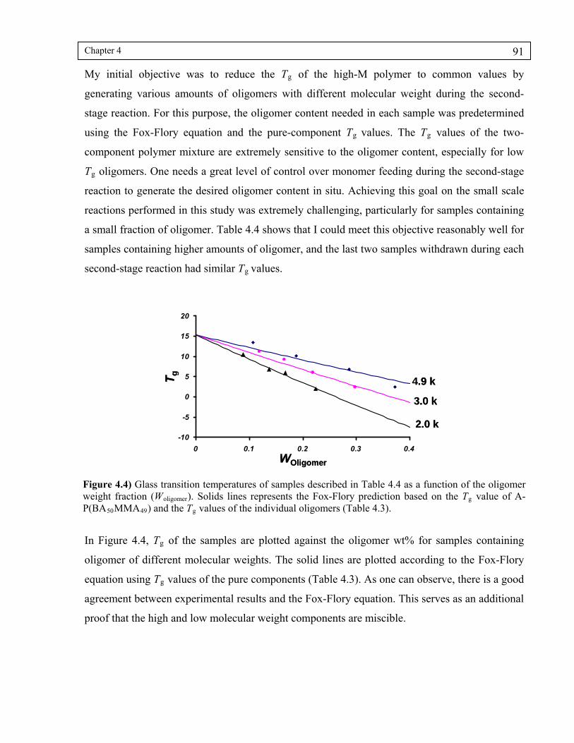
Chapter 4 91
My initial objective was to reduce the Tg of the high-M polymer to common values by
generating various amounts of oligomers with different molecular weight during the second-
stage reaction. For this purpose, the oligomer content needed in each sample was predetermined
using the Fox-Flory equation and the pure-component Tg values. The Tg values of the two-
component polymer mixture are extremely sensitive to the oligomer content, especially for low
Tg oligomers. One needs a great level of control over monomer feeding during the second-stage
reaction to generate the desired oligomer content in situ. Achieving this goal on the small scale
reactions performed in this study was extremely challenging, particularly for samples containing
a small fraction of oligomer. Table 4.4 shows that I could meet this objective reasonably well for
samples containing higher amounts of oligomer, and the last two samples withdrawn during each
second-stage reaction had similar Tg values.
-10
-5
0
5
10
15
20
0 0.1 0.2 0.3 0.4
Tg
3.0 k
2.0 k
WOligomer
4.9 k
-10
-5
0
5
10
15
20
0 0.1 0.2 0.3 0.4
Tg
3.0 k
2.0 k
WOligomer
4.9 k
Figure 4.4) Glass transition temperatures of samples described in Table 4.4 as a function of the oligomer weight fraction (Woligomer). Solids lines represents the Fox-Flory prediction based on the Tg value of A-P(BA50MMA49) and the Tg values of the individual oligomers (Table 4.3).
In Figure 4.4, Tg of the samples are plotted against the oligomer wt% for samples containing
oligomer of different molecular weights. The solid lines are plotted according to the Fox-Flory
equation using Tg values of the pure components (Table 4.3). As one can observe, there is a good
agreement between experimental results and the Fox-Flory equation. This serves as an additional
proof that the high and low molecular weight components are miscible.

Chapter 4 92
4.4.3 Effect of oligomer on the diffusion rate of high molecular weight polymers
To study interparticle polymer diffusion, I prepared films from a 1:9 mixture of D- and A-
containing particles. Aliquots of these dispersions were dried on small quartz plates at low
humidity and at 10 °C to yield thin (ca. 50 µm) and crack-free films. The drying process took ca.
15 min. After the film appeared dry to the naked eye, their donor fluorescence decay profiles
were measured. Measuring each decay took less that 2 min. After recording the initial decay, the
films were sealed in hermetically sealed chambers with a fixed humidity of 22% and were stored
in the dark at 25°C for the rest of the experiment. The relative humidity was kept constant by
using a saturated salt solution of potassium acetate.
The films were removed periodically from the sealed chamber and their fluorescence decays
were measured. I compared each decay with a series of simulated decays to find in turn the best
representative decay profile and the quantum efficiency of energy transfer (ΦET). Values of fm
were calculated via eq 2.25, Chapter 2 using simulated values for ΦET (0) and ΦET(∞). It is
difficult to achieve ΦET(0) experimentally since some polymer diffusion occurs during the
drying process. The extent of mixing measured from the initial decay was never zero for films
studied here. In all cases, ΦET(∞) values obtained from THF cast films were close to the
simulated value.
asing the amount of oligomer
leads to a faster growth in mixing fraction during the aging time.
In Figure 4.5A, I plot the evolution of fm as a function of annealing time for mixtures containing
two-component particles loaded with oligomer synthesized with 11 wt% C12-SH in the second
stage recipe. The same amount of C12-SH resulted in oligomers with Mn 2000 g/mol when
PMMA seed dispersion was used. In Figure 4.5A I compare films containing different amounts
of this oligomer (8.8, 13.6, 16.7 and 22.4 wt %). For comparison, I show results for an oligomer-
free (0 wt% oligomer) latex film. Initially, fm increases rapidly followed by a slow and gradual
increase during subsequent annealing. The results show that incre

Chapter 4 93
0
0.1
0.2
0.3
0.4
0.5
0.6
0.7
0 5000 10000 15000 20000 25000
fm
Time (min)
8.8
13.6
16.722.4
0
wt% Mn~2.0 k oligomer
A)
0 0.1 0.2 0.3 0.4 0.5 0.6 0.7
Dap
p(c
m2 /
min
)
fm
10-21
10-19
10-17
10-15
M
8.8 13.6 16.722.4
0
wt% Mn~2.0 k oligomerB)
Figure 4.5) FRET results for samples prepared by in situ generation of oligomer with 11% C12-SH added to the second reaction recipe. A) Fraction of mixing fm as a function of aging time for samples containing different amounts of the oligomer. B) Apparent diffusion coefficient Dapp as a function of fm for samples containing different amounts of the oligomer. The lowermost curve labeled “M” is the master curve prepared by shifting the data toward 0% curve. The master curve was moved one unit down for clarity. All lines are guides for the eye.
To quantify the extent by which the diffusion rate was enhanced in each sample, I employed a
master curve analysis. First, I calculated apparent diffusion coefficient (Dapp) values by assuming
a Fickian diffusion model as described in Chapter 2.5,29 The data in Figure 4.5B show that Dapp
values decreases as the fraction of mixing increases. This is a reflection of polydispersity of
labeled polymer molecules inside the particles. The Dapp value at each time is a cumulative
average of diffusion coefficients of all species that have participated in the diffusion process up
to that time. We have shown that although Dapp values are not true center of mass diffusion
coefficients, they closely follow the changes in diffusion rate of polymer molecules.29 Initially,
dye-labeled low-M species dominated the diffusion process, and therefore I recorded a high Dapp

Chapter 4 94
value. As diffusion progressed, higher-M slower diffusing species contributed to the increase in
fm, and thus Dapp decreased.
0
0.1
0.2
0.3
0.4
0.5
0.6
0.7
0 5000 10000 15000 20000 25000
fm
Time (min)
wt% Mn~3.0 k oligomer
11.916.521.9
29.8
0
A)
11.916.521.9
29.8
0
0
0.1
0.2
0.3
0.4
0.5
0.6
0.7
0 5000 10000 15000 20000 25000
fm
Time (min)
10.718.728.637.3
0
wt% Mn~4.9 k oligomer:B)
Figure 4.6) Plots of the mixing fraction vs annealing time for samples to which different amounts of oligomers with A) Mn = 3k and B) Mn = 4.9k were incorporated in situ.
In Figure 4.5B, I built a master curve using the oligomer-free curve as a reference. I applied a
vertical shift factor (aoligo) to Dapp values recorded for other samples to overlay them on the curve
recorded for 0% oligomer. These shift factors quantify the extent by which addition of the
oligomer accelerates the diffusion rate. My results show that for the sample that contained 22.4
wt% of the 2.0k oligomer, the rate of polymer diffusion was increased by a factor of ca. 25.
4.4.4 Effect of oligomer molecular weight on diffusion rate
My next objective was to compare the effect of oligomer molecular weight on its role as a
diffusion promoter. I changed the molecular weight of the oligomer by adding different amounts
of chain transfer agent (C12-SH) in the second stage reaction designed to synthesize two-
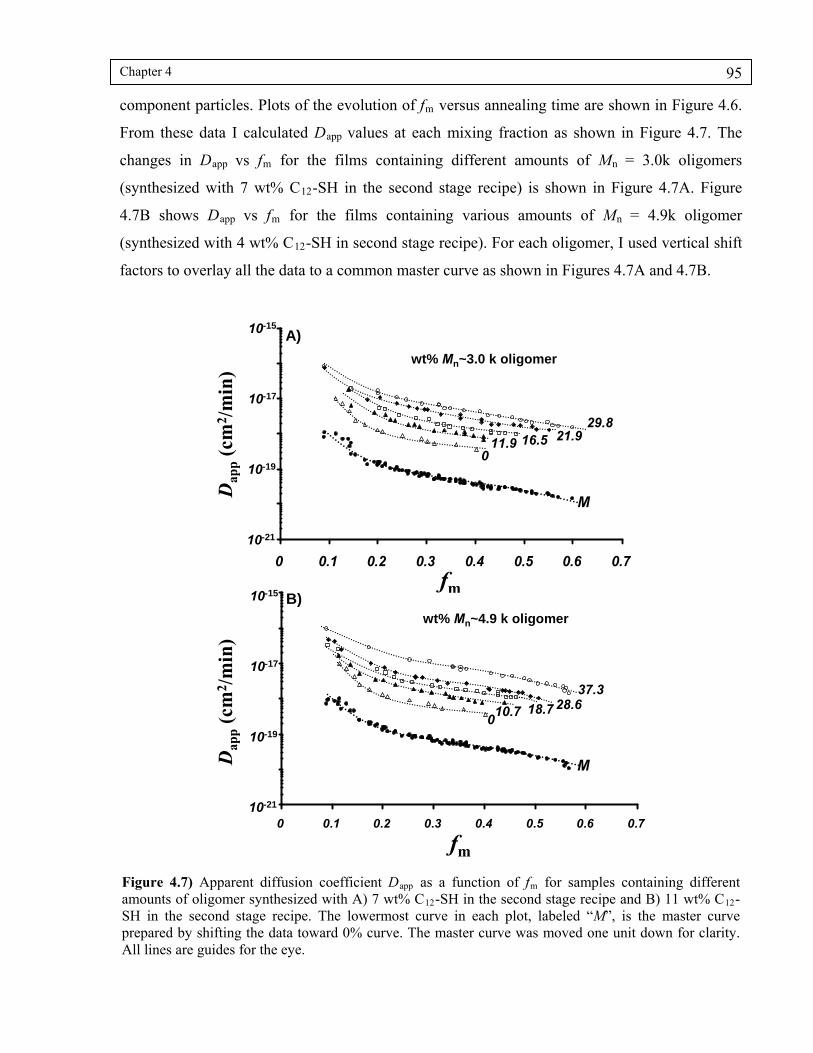
Chapter 4 95
component particles. Plots of the evolution of fm versus annealing time are shown in Figure 4.6.
From these data I calculated Dapp values at each mixing fraction as shown in Figure 4.7. The
changes in Dapp vs fm for the films containing different amounts of Mn = 3.0k oligomers
(synthesized with 7 wt% C12-SH in the second stage recipe) is shown in Figure 4.7A. Figure
4.7B shows Dapp vs fm for the films containing various amounts of Mn = 4.9k oligomer
(synthesized with 4 wt% C12-SH in second stage recipe). For each oligomer, I used vertical shift
factors to overlay all the data to a common master curve as shown in Figures 4.7A and 4.7B.
0 0.1 0.2 0.3 0.4 0.5 0.6 0.7
Dap
p(c
m2 /
min
)
fm
10-21
10-19
10-17
10-15
M
wt% Mn~3.0 k oligomer
11.9 16.5 21.929.8
0
A)
0 0.1 0.2 0.3 0.4 0.5 0.6 0.7
Dap
p(c
m2 /
min
)
fm
10-21
10-19
10-17
10-15
M
10.7 18.7 28.637.3
0
wt% Mn~4.9 k oligomer
B)
Figure 4.7) Apparent diffusion coefficient Dapp as a function of fm for samples containing different amounts of oligomer synthesized with A) 7 wt% C12-SH in the second stage recipe and B) 11 wt% C12-SH in the second stage recipe. The lowermost curve in each plot, labeled “M”, is the master curve prepared by shifting the data toward 0% curve. The master curve was moved one unit down for clarity. All lines are guides for the eye.

Chapter 4 96
The master curves shown in Figure 4.5B and Figures 4.7A and 4.7B have a common shape and
span over the same diffusion coefficient range of ca. 10-17 and 10-19 cm2/min. The master curve
shape reveals the details of molecular weight and molecular weight distribution of diffusing
species (labeled-molecules). I designed these experiments in such a way that in all samples the
mixing between the same labeled polymer molecules was followed. The similar shape of master
curves illustrates the success of my experimental design and that the molecular weight
distribution of labeled molecules did not significantly change during the second stage reaction.
Table 4.5. Vertical shift factors (aoligo) obtained from master curve analysis for samples containing different amounts of oligomers with various Mn.
2.0k 3.0k 4.9k Oligomer Mn :
wt% aoligo wt% aoligo wt% aoligo
8.8 3.1 11.9 2.3 10.7 2.1
13.6 6.8 16.5 3.7 18.7 3.7
16.7 12.2 21.9 6.9 28.6 4.9
22.4 24.5 29.8 10.5 37.3 13.5
In Table 4.5, I list the shift factors obtained by the master curve analysis as well as the total
amount of oligomer in each film. At a constant oligomer fraction, I obtained a higher shift factor
for the oligomer with lower molecular weight. For instance, when ca. 22 wt% of Mn = 2.0k
oligomer was used, I calculated an aoligo value of 24.4 whereas I obtained a value of only 6.9
when approximately the same amount of oligomer with Mn = 3.0k was used. The magnitude of
the shift factors represents the extent of plasticization by oligomers (oligoplasticization).
If oligoplasticization is due to an increase in the free-volume of the polymer blend, one would
expect the data to fit the Fujita-Doolittle model (eq 4.4).30 This model is based on the assumption
that the fractional free volume available for diffusion increases linearly with the volume fraction
of added plasticizer.
)1
.()T(
)T,0(f)T,0(f
)aln(
1
))0,T(D),T(Dln(
1
oligo
2
oligooligo
(4.4)
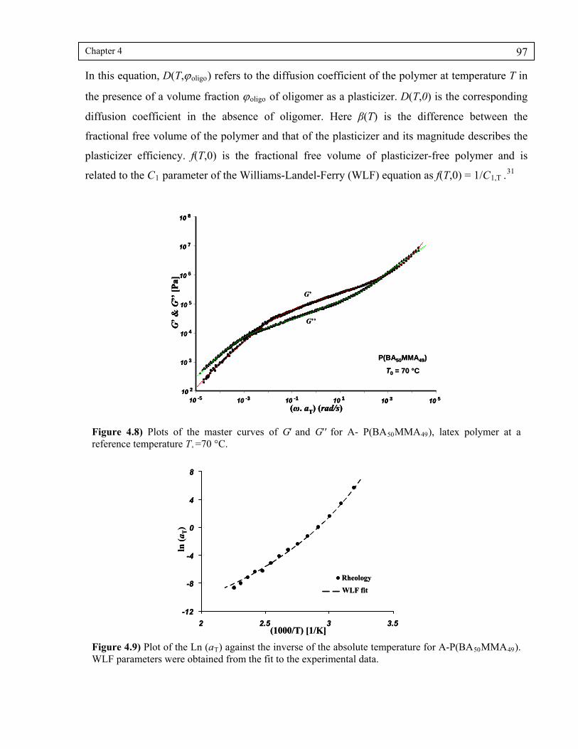
Chapter 4 97
In this equation, D(T,oligo) refers to the diffusion coefficient of the polymer at temperature T in
the presence of a volume fraction oligo of oligomer as a plasticizer. D(T,0) is the corresponding
diffusion coefficient in the absence of oligomer. Here β(T) is the difference between the
fractional free volume of the polymer and that of the plasticizer and its magnitude describes the
plasticizer efficiency. f(T,0) is the fractional free volume of plasticizer-free polymer and is
related to the C1 parameter of the Williams-Landel-Ferry (WLF) equation as f(T,0) = 1/C1,T .31
10 8
10 7
10 6
10 5
10 4
10 3
10 2
10 -5 10 -3 10 -1 10 1 10 3 10 5
G’
& G
’’[P
a]
(ω. aT) (rad/s)
P(BA50MMA49)
T0 = 70 °C
G’
G’’
10 8
10 7
10 6
10 5
10 4
10 3
10 2
10 -5 10 -3 10 -1 10 1 10 3 10 5
G’
& G
’’[P
a]
(ω. aT) (rad/s)
10 8
10 7
10 6
10 5
10 4
10 3
10 2
10 -5 10 -3 10 -1 10 1 10 3 10 5
G’
& G
’’[P
a]
(ω. aT) (rad/s)
P(BA50MMA49)
T0 = 70 °C
G’
G’’
Figure 4.8) Plots of the master curves of Gand Gfor A- P(BA50MMA49), latex polymer at a reference temperature T 0 =70 °C.
-12
-8
-4
0
4
8
2 2.5 3 3.5
ln(a
T)
(1000/T) [1/K]
Rheology
WLF fit
-12
-8
-4
0
4
8
2 2.5 3 3.5
ln(a
T)
(1000/T) [1/K]
Rheology
WLF fit
Figure 4.9) Plot of the Ln (aT) against the inverse of the absolute temperature for A-P(BA50MMA49). WLF parameters were obtained from the fit to the experimental data.

Chapter 4 98
To obtain the WLF parameters I constructed a rheology master curve for the same A-
P(BA50MMA49) sample used for the FRET measurements. I performed oscillatory shear
measurements at various temperatures and then applied time temperature superposition (TTS)
shift factors using the curve obtained at 70 °C as the reference. The master curve built by shifting
storage (G’) and loss modulus (G’’) is presented in Figure 4.8. Figure 4.9 shows that the TTS
shift factors obtained in this way fit the WLF equation reasonably well. From the fit, I obtained
WLF parameters at 70 °C to be C1, 70°C = 18.5 and C2 =129.4. To obtain f(25 °C, 0) I calculated
C1,25°C at 25 °C to be 28.3. Therefore, f(25 °C,0) = 1/C1,25°C = 0.035.
y = 0.114x + 0.035
R2 = 0.990
0
0.35
0.7
1.05
1.4
0 2 4 6 8 10 12
B)
1/L
n(a
olig
o)
β= 0.011
φoligo-1
y = 0.0661x + 0.0353
R2 = 0.9617
0
0.25
0.5
0.75
1
0 2 4 6 8 10 12
C)
β= 0.019
1/L
n(a
oli
go)
φoligo-1
y = 0.132x + 0.035
R2 = 0.984
0
0.4
0.8
1.2
1.6
0 2 4 6 8 10 1
A)
1/L
n(a
olig
o)
φoligo-1
β= 0.009
2
A)
B)
C)
Figure 4.10) Plots of 1/Ln(aoligo) vs φoligo-1 based on the data presented in Table 4.5 for in situ
incorporation of oligomers with A) Mn=2.0k, the slope of the line is 0.066 (R2=0.96); B) Mn=3.0k, the slope of the line is 0.114 (R2=0.99); C) Mn=4.9k, the slope of the line is 0.132 (R2=0.96).
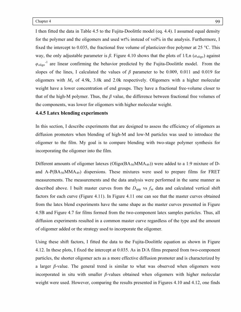
Chapter 4 99
I then fitted the data in Table 4.5 to the Fujita-Doolittle model (eq. 4.4). I assumed equal density
for the polymer and the oligomers and used wt% instead of vol% in the analysis. Furthermore, I
fixed the intercept to 0.035, the fractional free volume of plasticizer-free polymer at 25 °C. This
way, the only adjustable parameter is β. Figure 4.10 shows that the plots of 1/Ln (aoligo) against
φoligo-1 are linear confirming the behavior predicted by the Fujita-Doolittle model. From the
slopes of the lines, I calculated the values of β parameter to be 0.009, 0.011 and 0.019 for
oligomers with Mn of 4.9k, 3.0k and 2.0k respectively. Oligomers with a higher molecular
weight have a lower concentration of end groups. They have a fractional free-volume closer to
that of the high-M polymer. Thus, the β value, the difference between fractional free volumes of
the components, was lower for oligomers with higher molecular weight.
4.4.5 Latex blending experiments
In this section, I describe experiments that are designed to assess the efficiency of oligomers as
diffusion promoters when blending of high-M and low-M particles was used to introduce the
oligomer to the film. My goal is to compare blending with two-stage polymer synthesis for
incorporating the oligomer into the film.
Different amounts of oligomer latexes (Oligo(BA50MMA49)) were added to a 1:9 mixture of D-
and A-P(BA50MMA49) dispersions. These mixtures were used to prepare films for FRET
measurements. The measurements and the data analysis were performed in the same manner as
described above. I built master curves from the Dapp vs fm data and calculated vertical shift
factors for each curve (Figure 4.11). In Figure 4.11 one can see that the master curves obtained
from the latex blend experiments have the same shape as the master curves presented in Figure
4.5B and Figure 4.7 for films formed from the two-component latex samples particles. Thus, all
diffusion experiments resulted in a common master curve regardless of the type and the amount
of oligomer added or the strategy used to incorporate the oligomer.
Using these shift factors, I fitted the data to the Fujita-Doolittle equation as shown in Figure
4.12. In these plots, I fixed the intercept at 0.035. As in D/A films prepared from two-component
particles, the shorter oligomer acts as a more effective diffusion promoter and is characterized by
a larger β-value. The general trend is similar to what was observed when oligomers were
incorporated in situ with smaller β-values obtained when oligomers with higher molecular
weight were used. However, comparing the results presented in Figures 4.10 and 4.12, one finds
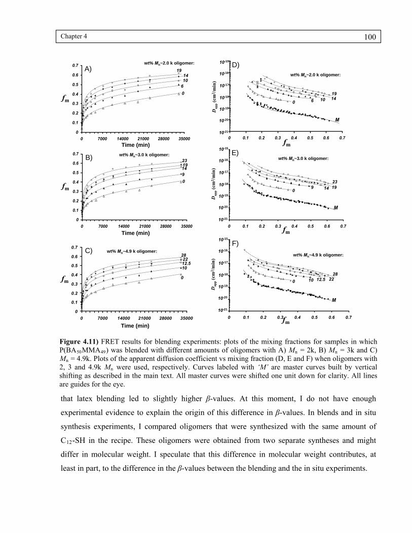
Chapter 4 100
that latex blending led to slightly higher β-values. At this moment, I do not have enough
experimental evidence to explain the origin of this difference in β-values. In blends and in situ
synthesis experiments, I compared oligomers that were synthesized with the same amount of
C12-SH in the recipe. These oligomers were obtained from two separate syntheses and might
differ in molecular weight. I speculate that this difference in molecular weight contributes, at
least in part, to the difference in the β-values between the blending and the in situ ex
0 0.1 0.2 0.3 0.4 0.5 0.6 0.7
Dap
p(c
m2 /
min
)
fm
10-21
10-20
10-19
10-18
10-17
10-16
10-15
M
10 12.5 2228
0
wt% Mn~4.9 k oligomer:
0
0.1
0.2
0.3
0.4
0.5
0.6
0.7
0 7000 14000 21000 28000 35000
fm
Time (min)
wt% Mn~4.9 k oligomer:
1012.522
28
0
0 0.1 0.2 0.3 0.4 0.5 0.6 0.7
Dap
p(c
m2 /
min
)
fm
10-21
10-20
10-19
10-18
10-17
10-16
10-15
M
wt% Mn~3.0 k oligomer:
09 14 19
23
0
0.1
0.2
0.3
0.4
0.5
0.6
0.7
0 7000 14000 21000 28000 35000
fm
Time (min)
wt% Mn~3.0 k oligomer:
0
9141923
0 0.1 0.2 0.3 0.4 0.5 0.6 0.7
Dap
p(c
m2 /
min
)
fm
10-21
10-20
10-19
10-18
10-17
10-16
10-15
M
6 10 1419
0
wt% Mn~2.0 k oligomer:
0
0.1
0.2
0.3
0.4
0.5
0.6
0.7
0 7000 14000 21000 28000 35000
fm
Time (min)
61014
19
0
wt% Mn~2.0 k oligomer:
A)
B)
C)
D)
E)
F)
Figure 4.11) FRET results for blending experiments: plots of the mixing fractions for samples in which P(BA50MMA49) was blended with different amounts of oligomers with A) Mn = 2k, B) Mn = 3k and C) Mn = 4.9k. Plots of the apparent diffusion coefficient vs mixing fraction (D, E and F) when oligomers with 2, 3 and 4.9k Mn were used, respectively. Curves labeled with ‘M’ are master curves built by vertical shifting as described in the main text. All master curves were shifted one unit down for clarity. All lines are guides for the eye.
periments.

Chapter 4 101
y = 0.078x + 0.035
R2 = 0.984
0
0.25
0.5
0.75
1
0 2 4 6 8 10 1
B)
φoligo-1
1/L
n(a
olig
o)
2
β= 0.016
y = 0.051x + 0.035
R2 = 0.983
0
0.25
0.5
0.75
1
0 5 10 15 20
A)
φoligo-1
1/L
n(a
olig
o)
β= 0.024
y = 0.087x + 0.035
R2 = 0.957
0
0.25
0.5
0.75
1
0 2 4 6 8 10
C)
12φoligo
-1
1/L
n(a
olig
o)
β= 0.014
Figure 4.12) Plots of 1/Ln(aoligo) vs φoligo-1 for films prepared by blending oligomers of different Mn A)
Mn=2.0k, the slope of the line is 0.057 (R2=0.98); B) Mn=3.0k, the slope of the line is 0.078 (R2=0.98);
4.4.6 Effect of oligomer on polymer rheological properties
To examine the influence of the molecular weight of incorporated oligomers on polymer flow
properties at a common temperature, it is necessary to compare samples with the same Tg. Blend
samples with a common Tg will contain different amounts of oligomer depending on Mn of the
oligomer. For this purpose, I chose two-component samples to which 20 wt% of the 2.0k
oligomer, 30 wt% of the 3.0k oligomer and 40 wt% of the 4.9k oligomer were incorporated in
situ. These samples have a common Tg value of ca. 2 °C as shown in Table 4.4. I measured the
changes in shear viscosity (η) at various shear rates ( ) for these samples at a constant
temperature of 100 ± 1°C as shown in Figure 4.13. These measurements were carried out at a
temperature well above Tg in order to soften the polymer and to obtain meaningful flow curves.
The measurement temperature corresponds to a (Texp-Tg) of ca. 98 °C. For comparison, I studied

Chapter 4 102
the flow behavior of unmodified A-P(BA50MMA49). This polymer has a higher Tg value than the
two-component samples (15.5°C). For this sample, the measurement was performed at 113 ± 1
°C, at the same value of (Texp-Tg), to compensate for the effect of Tg on viscosity.
1000
10000
100000
0.01 0.1 1 10 100Shear rate (s-1)
η(P
a.s
)
4.9k (40 wt%)
3.0k (30 wt%)
2.0k (20 wt%)
A-P(BA50MMA49)
1000
10000
100000
0.01 0.1 1 10 100Shear rate (s-1)
η(P
a.s
)
4.9k (40 wt%)
3.0k (30 wt%)
2.0k (20 wt%)
A-P(BA50MMA49)
Figure 4.13) Plots of shear viscosity (η) as a function of shear rate for A-P(BA50MMA49) at 113 °C; and for the two-component samples to which 20 wt% of the 2.0k oligomer; 30 wt% of the 3.0k oligomer and 40 wt% of the 4.9k oligomer was incorporated. The measurements on the two-component samples were performed at 100 °C. The lines represent best-fit curve according to the Cross model. 35
The flow curves shown in Figure 4.13 represent typical behavior of entangled polymer chains
under shear flow. At low shear rates the viscosity was constant (zero shear rate viscosity, η0) and
the fluid exhibited a pseudo-Newtonian behavior. When shear the rate exceeded a critical value,
shear-thinning was observed.
Above a critical molecular weight (Me), the effect of neighbor chains on molecular motion can
no longer be expressed in terms of simple frictional forces. Shear flow can break the physical
entanglement network.32 At low shear rates, entanglement formation by Brownian motion
competes with shear induced disentanglement to maintain the entanglement density, and the
viscosity remains constant. When shear rate exceeds a critical value, the rate of entanglement
formation can no longer keep up with shear induced disentanglement, and thus viscosity
decreases with shear rate. For samples with high polydispersity in molecular weight, the shear-
thinning behavior commences at lower shear rates and the transitional region between Newtonian
and non-Newtonian regime broadens.33 ,34
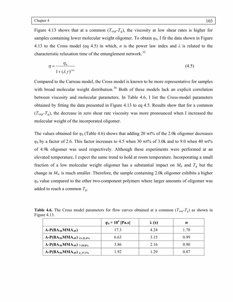
Chapter 4 103
Figure 4.13 shows that at a common (Texp-Tg), the viscosity at low shear rates is higher for
samples containing lower molecular weight oligomer. To obtain η0, I fit the data shown in Figure
4.13 to the Cross model (eq 4.5) in which, n is the power law index and λ is related to the
characteristic relaxation time of the entanglement network.35
)(.
0
)(1 n
(4.5)
Compared to the Carreau model, the Cross model is known to be more representative for samples
with broad molecular weight distribution.36 Both of these models lack an explicit correlation
between viscosity and molecular parameters. In Table 4.6, I list the Cross-model parameters
obtained by fitting the data presented in Figure 4.13 to eq 4.5. Results show that for a common
(Texp-Tg), the decrease in zero shear rate viscosity was more pronounced when I increased the
molecular weight of the incorporated oligomer.
The values obtained for η0 (Table 4.6) shows that adding 20 wt% of the 2.0k oligomer decreases
η0 by a factor of 2.6. This factor increases to 4.5 when 30 wt% of 3.0k and to 9.0 when 40 wt%
of 4.9k oligomer was used respectively. Although these experiments were performed at an
elevated temperature, I expect the same trend to hold at room temperature. Incorporating a small
fraction of a low molecular weight oligomer has a substantial impact on Mn and Tg but the
change in Mw is much smaller. Therefore, the sample containing 2.0k oligomer exhibits a higher
η0 value compared to the other two-component polymers where larger amounts of oligomer was
added to reach a common Tg.
Table 4.6. The Cross model parameters for flow curves obtained at a common (Texp-Tg) as shown in Figure 4.13.
η0 × 104 [Pa.s] λ (s) n
A-P(BA50MMA49) 17.3 4.24 1.78
A-P(BA50MMA49) 11-22.4% 6.63 3.15 0.99
A-P(BA50MMA49) 7-29.8% 3.86 2.16 0.90
A-P(BA50MMA49) 4_37.3% 1.92 1.29 0.87

Chapter 4 104
In Figure 4.13, the flow curves for the oligomer-free sample and the samples containing lower
molecular weight oligomers stop at a lower shear rate value. At this shear rate, the Normal forces
exceeded the instrument threshold value (1500 g), and data acquisition was terminated
automatically. Normal stress difference in steady shear flow represents coupling between elastic
and viscous effects at high shear rates. For all samples except the sample containing the 4.9k
oligomer, the final shear rate was limited by the generation of normal forces. This reflects the
lower entanglement density in the sample containing relatively large amounts of the longest
oligomers (4.9k).
4.5 Summary
I synthesized two-component polymer particles consisting of a miscible polymer blend, a high-M
A-P(BA50MMA49) and an oligomer with the same composition as the high-M polymer but with
distinctly higher concentration of the end groups. I measured the amount of oligomer in each
sample via a calibration curve based on the UV absorbance of the acceptor chromophore as well
as from the Förster equation. These methods resulted in reasonably close values.
I showed that the oligomers were miscible with the high-M polymer for all samples studied here.
I followed the rate of mixing between high molecular weight polymers in the presence of various
amounts of oligomers with different molecular weight using fluorescence resonance energy
transfer (FRET) technique. In freshly formed latex films, the oligomers became uniformly
distributed rapidly after coalescence. The experiments were designed in such a way that in all
samples diffusion between the same labeled chains was followed. The results showed that master
curves built from different samples had a common shape. I could fit the shift factors obtained by
building master curves to the Fujita-Doolittle equation and show that lower molecular weight
oligomers act more efficiently as a diffusion promoter. For in situ incorporated oligomers with
Mn = 2.0k a β-value of 0.019 was obtained. When the 2.0k oligomer was introduced to the film
via latex blending, a larger β-value of 0.024 was obtained. Traditional VOC additives such as
2,2,4-trimethyl-1,3-pentanediol monoisobutyrate (Texanol™, TPM) have a higher β-value
(0.07).37
To study the consequences of oligomer addition on the follow properties of the two-component
polymers, I measured the flow curves of samples that had a common Tg value of 2 °C. To
decrease Tg to this common value, I needed to incorporate a larger amount of the oligomers with
Chapter 4 105
higher molecular weight. I studied samples that contained ca. 20 wt% of the 2.0k oligomer, 30
wt% of the 3.0k oligomer and 40 wt% of the 4.9k oligomer. For comparison, I obtained the flow
curve of the one-component P(BA50MMA49) which had a higher Tg value. To compensate for
the effect of temperature on viscosity, I performed this measurement at a higher temperature that
gave the same (Texp-Tg = 98 °C) as the measurements performed on the two-component
polymers. The results showed that incorporating 20 wt% of the 2.0k oligomer reduced the zero
shear rate viscosity of P(BA50MMA49) by a factor of 2.6. Incorporating longer oligomers led to a
more pronounced decrease in the zero shear rate viscosity. Oligomers with higher molecular
weight had a greater impact on decreasing Mw. Moreover, the entanglement density was lower in
sample containing oligomers with higher molecular weight since a larger amount of the oligomer
was needed to decrease the glass transition to a common value of 2 °C.
I conclude that oligomers with low molecular weight are more efficient as a diffusion promoter
compared to their higher molecular weigh counterparts. Oligomers that have higher molecular
weight act more efficiently in decreasing polymer viscosity. Therefore, they might serve as non-
volatile coalescing aid additives which facilitate particle deformation in response to forces
generated by water evaporation. The deleterious drawback of adding high molecular weigh
oligomer is lower viscosity of the final polymer film.

Chapter 4 106
4.6 References
1 a) Asua JM. Polymeric dispersions : principles and applications. Dordrecht; Boston: Kluwer
Academic, 1997; b) Udagama, R.; Degrandi-Contraires, E.; Creton, C.; Graillat, C.; McKenna,
T. F. L.; Bourgeat-Lami, E. Macromolecules 2011, 44, 2632-2642.; c) Udagama, R.; Degrandi-
Contraires, E.; Creton, C.; Graillat, C.; McKenna, T. F. L.; Bourgeat-Lami, E. Macromolecules
2011, 44, 2632-2642.
2 a) Chung, G.-C.; Kornfield, J. A.; Smith, S. D. Macromolecules 1994, 27, 5729-5741. b)
Kamath, S.; Colby, R. H.; Kumar, S. K. Macromolecules 2003, 36, 8567-8573. c) Hirose, Y.;
Adachi, K. Macromolecules 2006, 39, 1779-1789. d) Mpoukouvalas, K.; Floudas, G.
Macromolecules 2008, 41, 1552-1559.
3 a) Ueberreiter, K.; Kanig, G. J. Colloid Sci. 1952, 7, 569-583.b) Couchman, P. R. J. Mater. Sci.
1980, 15, 1680-1683.
4 Masaro, L.; Zhu, X. . Prog. Polym. Sci. 1999, 24, 731-775.
5Soleimani, M.; Haley, J. C.; Lau, W.; Winnik, M. A. Macromolecules 2010, 43, 975-985.
6 Liu, Y. Q.; Haley, J. C.; Deng, K.; Lau, W.; Winnik, M. A. Macromolecules 2007, 40, 6422.
7 Rubinstein M and Colby RH. Polymer physics. Oxford; New York: Oxford University Press,
2003.
8 Graessley, W. W. J. Polym. Sci., Part B: Polym. Phys. 1980, 18, 27-34.
9 Pechhold, W.; Vonsoden, W.; Stoll, B. Macromol. Chem. Phys. 1981, 182 (2), 573-581.
10 a) Masuda, T.; Kitagawa, K.; Inoue, T.; Onogi, S. Macromolecules 1970, 3, 116. b) Graessley,
W. W.; Segal, L. Macromolecules 1969, 2, 49.
11Odrobina, E.; Feng, J.; Winnik, M. A. J. Polym. Sci., Part A: Polym. Chem. 2000, 38, 3933.

Chapter 4 107
12Tomba, J. P.; Ye, X.; Li, F.; Winnik, M. A.; Lau, W. Polymer 2008, 49, 2055.
13Tzitzinou, A.; Keddie, J. L.; Geurts, J. M.; Peters, A.; Satguru, R. Macromolecules 2000, 33,
2695.
14 Fasano, D. M.; Fitzwater, S. J.; Lau, W.; Sheppard, A. C. Can. J. Chem. 2010, 88, 500.
15Kulka, M. J. Am. Chem. Soc. 1954, 76, 5469.
16Elizalde, O.; Arzamendi, G.; Leiza, J. R.; Asua, J. M. Ind. Eng. Chem. Res. 2004, 43, 7401.
17Greenspan, L. J. Res. Natl. Bur. Stand., Sect. A 1977, 81, 89.
18 Becker W, Castleman AW, Toennies JP, and Zinth W. Advanced Time-Correlated Single
Photon Counting Techniques. Berlin, Heidelberg: Springer Verlag Berlin Heidelberg, 2005.
19 James, D. R.; Demmer, D. R. M.; Verrall, R. E.; Steer, R. P. Rev. Sci. Instrum. 1983, 54, 1121.
20 a) Kramer, E. J.; Green, P.; Palmstrøm, C. J. Polymer 1984, 25, 473-480. b) Jordan, E. A.;
Ball, R. C.; Donald, A. M.; Fetters, L. J.; Jones, R. A. L.; Klein, J. Macromolecules 1988, 21,
235.
21 Kausch, H. H.; Tirrell, M. Annu. Rev. Mater. Sci. 1989, 19, 341.
22 Gennes P-Gd. Scaling concepts in polymer physics. Ithaca, N.Y.: Cornell University Press,
1979.
23 Echevarria, A.; Leiza, J. R.; de la Cal, J. C.; Asua, J. M. AIChE J. 1998, 44, 1667.
24 Vail, N. K.; Barlow, J. W.; Beaman, J. J.; Marcus, H. L.; Bourell, D. L. J. Appl. Polym. Sci.
1994, 52, 789.
25 Brandrup J and Immergut EH. Polymer handbook. New York: Wiley, 2003.
26 Uraneck, C. A.; Burleigh, J. E. J. Appl. Polym. Sci. 1973, 17, 2667.

Chapter 4 108
27 Sayer, C.; Lima, E. L.; Pinto, J. C.; Arzamendi, G.; Asua, J. M. J. Polym. Sci., Part A: Polym.
Chem. 2000, 38, 367.
28 Lau, W. Macromol. Symp. 2002, 182, 283.
29 Farinha, J. P. S.; Martinho, J. M. G.; Yekta, A.; Winnik, M. A. Macromolecules 1995, 28,
6084.
30 Fujita, H. Fortschr. Hochpolym-Forsch 1961, 3,1-47.
31 Ferry JD. Viscoelastic properties of polymers. 3rd ed. New York: John Wiley & Sons; 1980.
32 a) Graessley, W. W. J. Chem. Phys. 1965, 43, 2696. b) Graessley, W. W. The entanglement
concept in polymer rheology; Springer-Verlag: Berlin; New York, 1974.
33 Graessley, W. W. J. Chem. Phys. 1967, 47, 1942.
34 Graessley, W. W.; Segal, L. AIChE J. 1970, 16, 261-267.
35 a) Cross, M. M. J. Appl. Polym. Sci.1969, 13, 765.b) Cross, M. M. J. Colloid Sci. 1965, 20,
417.
36 Hieber, C. A.; Chiang, H. H. Polym. Eng. Sci. 1992, 32, 931.
37 a) Juhué, D.; Wang, Y.; Lang, J.; Leung, O.-M.; Goh, M. C.; Winnik, M. A. J. Polym. Sci.,
Part B: Polym. Phys. 1995, 33, 1123-1133. b) Juhue, D.; Wang, Y. C.; Winnik, M. A.; Haley, F.
Makromol. Chem., Rapid Commun.1993, 14, 345.c) Schroeder, W. F.; Liu, Y. Q.; Tomba, J. P.;
Soleimani, M.; Lau, W.; Winnik, M. A. J. Phys. Chem. B 2010, 114, 3085.
Chapter 5 109
CHAPTER FIVE
Synthesis of Smart Polymer Nanoparticles and Their Application as
Environmentally Compliant Coatings i
5.1 Introduction
Smart polymers are defined as polymers that sense changes in their environment and respond to
these changes in useful ways.1 Among the stimuli to which polymers can respond are light,
temperature or pH changes,2 or the variation of electrical potential.3 Materials fabricated from
smart polymers are normally targeted for “high technology” applications in areas such as drug
delivery,4 biotechnology,5 sensors and optical displays.6 For systems that operate in solution,
one classic example is based upon thermosensitive microgels which undergo a volume phase
transition when heated above a critical temperature.7 Introduction of pH-sensitive functionalities
can shift the phase-transition temperature in a way that is pH dependent.8 These microgels are
being developed for drug-delivery applications.9
In this chapter, I describe a new class of colloidal polymer particles that undergo a reversible
change in morphology, from a uniform polymer blend to a core-shell structure, upon a change in
pH. These particles were designed to provide a new approach to pressing problems with (water-
based) latex paints. The essential feature of latex paints is that as an aqueous dispersion of
polymer nanoparticles dries, the particles fuse to form a continuous transparent and mechanically
robust film. This film acts as a binder to support TiO2 and other pigments on a substrate,
providing hiding, color, and protection from corrosion. The two issues that these novel latex
particles were designed to address are environmental concerns and performance.
Environmentally compliant coatings should form films as they dry with formulations that contain
little or no volatile organic compounds (VOCs). Soft polymer nanoparticles will do this, but they
i This chapter appeared as: “Smart Polymer Nanoparticles Designed for Environmentally Compliant Coatings” Soleimani, M.; Haley, J. C.; Majonis, D.; Guerin, G.; Lau, W.; Winnik, M. A. Journal of the American Chemical Society 2011, 133, 11299-11307.

Chapter 5 110
yield coatings that are tacky to the touch and have poor mechanical properties. This problem is
traditionally overcome with volatile plasticizers that are VOC components.
The performance property that remains a serious challenge for latex coatings is commonly
referred to as “open time”. Open time or “wet edge time” can be defined as the period of time
during which a painter can make corrections to the freshly applied wet paint film without leaving
brush marks.10,11 The edges of a paint film are thinner and will dry more rapidly than the bulk of
the film. If the edge becomes dry and subsequently repainted with a new layer of paint, the dried
edge will be visible and causes an irregularity at the paint surface. Solvent-based (e.g., alkyd)
coatings are much slower drying than latex coatings, and one has much longer time to rework the
edges of a painted area to achieve a smooth and uniform finish. For health reasons, however, and
a more general concern for the environment, solvent based coatings are being replaced by latex
paints. Since open time is not easily measured, it is difficult to assess except in a qualitative way.
Here I describe experiments carried out to investigate the potential for the new “smart” latex
particles to improve the normally short open time of latex coatings.
Figure 5.1. Film formation by soft polymer nanoparticles covered with an oligomeric shell a) before the end of water evaporation and b) after particles deformation. In our design, the shell can act as a temporary barrier to the onset of polymer diffusion across the interparticle boundaries.
The initial idea for a dispersion that can afford these properties was developed by Dr. Willie Lau
at Rohm and Hass (now Dow Chemicals), our industrial partner. In this design, the base latex
would have a typical composition for an architectural coating, a relatively high molecular weight
(high-M) poly(butyl acrylate-co-methyl methacrylate) (P(BA-MMA)) polymer with a monomer
ratio of 55/45 by weight (48.8 mol% BA) with a targeted glass transition temperature (Tg) of 7
C. These particles would be loaded with a second, low molecular weight polymer (oligomer)
with a much lower Tg. During my discussions with Dr. Lau, I decided to modify this original
design to make it amenable to quantitative studies. I modified the oligomer composition and
labeled the components with fluorescence dyes. In my design, the oligomeric material would

Chapter 5 111
contain carboxyl groups in the form of methacrylic acid, as well as styrene, methyl methacrylate
and butyl acrylate. The composition was designed to be molecularly miscible with the high-M
P(BA-MMA) when the carboxyl groups are protonated, but immiscible when they are
deprotonated. The styrene units prevent the carboxylate form of the oligomer from dissolving in
the aqueous phase. In this design, upon deprotonating the acid groups, the oligomer would be
neutralized and phase separate from the high-M base polymer to form a core-shell structure with
a shell rich in –COO(-) groups. As water evaporates from the particle dispersion and the particles
come into contact, one expects that the carboxylate-rich shell would form a water-swollen
membrane 12 as depicted schematically in Figure 5.1. This membrane would retard the final
stages of drying, delay the onset of coalescence, and thereby promote open time. If the counter
ions were NH4+, the final stages of drying would result in loss of ammonia to the atmosphere,
reprotonation of the carboxyl groups, and miscibility of the oligomer with the base polymer. The
miscible oligomer should, in turn, plasticize the base polymer and promote the diffusion of high-
M polymer across the interparticle boundaries. This is the event at the molecular level that leads
to strong interfaces and robust mechanical properties.
This chapter is organized as follow. First I describe the synthesis and characterization of these
smart particles and experiments performed to establish their morphology. Here I find a
remarkable and reversible morphology transformation from a core-shell structure in base to a
uniform blend in acidic solution. Second, I show that the protonated form of the oligomer does
indeed accelerate polymer diffusion in latex films. Finally, I demonstrate that in films formed
from these two-component latex nanoparticles neutralized with aqueous ammonia, there is a
significant retardation of nanoparticle coalescence, followed by loss of ammonia and
enhancement of polymer diffusion rate in the dry film.
5.2 Experimental
5.2.1 Materials
Potassium persulfate (KPS), 1-dodecyl mercaptan (C12-SH) and sodium dodecyl sulfate (SDS)
were purchased from Aldrich and used as received. Methyl-β-cyclodextrin (Me--CD, 50 % w/w
solution in water, Wacker Chemie) was used as a phase transfer catalyst. Methyl methacrylate
(MMA), Styrene (Sty), butyl acrylate (BA), and methacrylic acid (MAA) were purified from

Chapter 5 112
hydroquinone inhibitors by passing through an inhibitor remover column (Aldrich).
Phenanthrylmethyl methacrylate (PheMMA) was purchased from Toronto Research Chemicals
Inc. and used without further purification. Dimethylamino-2-methacryloxy-5-
methylbenzophenone (NBenMA) was synthesized as we described earlier. 13 Water was purified
by a Milli-Q ion exchange filtration system.
5.2.2 Nanoparticle synthesis
Seeded emulsion polymerization under monomer-starved conditions was used to synthesize
composite polymer particles. First a seed dispersion was prepared by conventional emulsion
polymerization. Appropriate amounts of water, SDS and MMA (Table 5.1) were stirred in a 250
mL three-neck flask equipped with an overhead mechanical stirrer and a condenser. The mixture
was bubbled with high purity nitrogen for 30 min and then immersed in 80 °C thermostated oil
bath. After thermal equilibration, the initiator solution was injected and the reaction was
continued for 45 min. 5 ml of this dispersion was taken from the flask with a deoxygenated
syringe for further analysis. The reaction was continued by feeding the first stage monomer
emulsion.
5.2.2.1 First stage seeded emulsion polymerization
A solution of the fluorescent dye in the monomer mixture was added to a solution of SDS in
water and shaken to form a stable monomer emulsion (Table 5.1). The initiator solution (150 mg
KPS in 3 gr water) was injected into the flask. Then, the monomer emulsion was fed to the flask
by a fluid metering pump (Drive: FMI-QG20, Head: RH0CKC) with a constant rate of ca. 150
μl/min for a total time of ~ 5 hours. The reaction was continued for an additional 30 min after
feeding all the monomer emulsion. For further analysis, 6.5 ml of the dispersion was taken from
the flask using a deoxygenated syringe. The reaction was continued by feeding the second stage
monomer emulsion.
5.2.2.2 Second stage seeded emulsion polymerization
The second seeded emulsion polymerization was designed to modify the former particles in situ
with a carboxylated oligomer. The oligomer was labeled either with the donor dye (the sample
used to study morphology at different pH values) or not labeled (the samples used to study its

Chapter 5 113
effect on the diffusion of the high-M polymer). To facilitate incorporation of MAA and prevent
its deprotonation, all the synthesis were performed in unbuffered water. The pH of the dispersion
prepared in this way was ca. 3.5. To facilitate transport of C12-SH, Me--CD was added to the
reaction as a phase transfer catalyst.14
I employed a stage ratio one of 1:1, i.e., the final particles consisted of 50 wt % high-M acceptor-
labeled polymer and 50 wt % donor-labeled oligomer. The second stage reaction was performed
in a similar manner to what was described above. The initiator solution was injected into the
flask followed by feeding the monomer emulsion (150 μl/min for a total time of 5 hours). After
the end of the feeding, the reaction was continued for another 30 min. Finally, the reaction
mixture was cooled in an ice bath and then opened to the atmosphere. The dispersions were
filtered through glass wool and stored in the dark in brown bottles. The solids content of the
dispersions were determined gravimetrically by freeze drying dispersions overnight.
Table 5.1. Synthesis of the dye-labeled composite particles
Seed (g) Core polymer(g) Oligomer loading (g)
BA — 13.75 12.38
MMA 2.34 11.25 2.25
Sty — — 3.37
MAA — — 2.25
Dye comomoner a,b — 0.200 a 0.522 b
C12-SH — 0.05 2.25
Me--CD — 0.05 0.35
Water 20.00 20.00 20.00
SDS 0.118 0.150 0.150
KPS 0.035 0.150 0.150
a. Dimethylamino-2-methacryloxy-5-methylbenzophenone (NBen)
b. Phenanthrylmethyl methacrylate
Chapter 5 114
5.2.3 Instrumentation and analysis
5.2.3.1 Fluorescence decay measurements
Fluorescence lifetime measurements were carried out on a single photon counting setup as
described in section 3.2.5, Chapter 3. To reduce the intensity of scattered light at the detector, a
335 nm cutoff filter was mounted on the emission monochromator. Data were collected until
10000 counts were accumulated in the maximum channel. The instrument-response-function
(IRF) was obtained by using a mimic standard (degassed solution of p-terphenyl, lifetime: 0.96
ns)15 following the protocol described in section 2.5, Chapter 2.
5.2.3.2 Dynamic Light Scattering (DLS)
DLS measurements were performed with an ALV/DLS/SLS-5000 Compact Goniometer System
equipped with a He-Ne laser ( λ0= 632.8 nm, 35 mW) emitting vertically polarized light as the
light source and a Dual ALV-High Q.E. APD avalanche photodiode module connected to an
ALV-5000/EPP multiple digital time correlator as the detection module. The samples were
prepared in sealed screw caped vials and equilibrated at the desired pH overnight. The samples
were placed in a thermostated cis-decahydronaphthalene vat which matched the index of
refraction of the glass vial.
5.2.3.3 Dispersion dialysis
The dispersion was diluted to ~ 1 wt% with deionized water and then washed with a Millipore
Lab scale TFF system equipped with a Cole Parmer Masterflex® L/S® pump and a Pellicon
cartridge (MWCO 300k). The dialysis was continued until the diffusate stream conductivity
reached below 15 µS/cm.
5.2.3.4 Differential Scanning Calorimetry (DSC)
Glass transition temperatures (Tg) of the polymers were measured using a TA2920 MDS. All the
samples were prepared from polymers that were freeze-dried over night. The samples were
equilibrated at -60 °C for 10 min and then scanned to 150°C with a ramp of 10°C/min for two
complete cycles. The Tg values reported here are taken as the mid-point temperature of the
inflection in the first heating cycle.

Chapter 5 115
5.2.3.5 Gel Permeation Chromatography (GPC)
Molecular weight and molecular weight distribution were determined by gel permeation
chromatography (GPC) using tetrahydrofuran (THF) as the eluent (flow rate: 0.6 ml/min) and a
Viscotek liquid chromatography instrument equipped with a Viscotek RI detector (VE3580) and
a Varian PLgel 5μm mixed-D columns. The UV signal was collected with a UV detector (VE
3210) at the maximum absorption of the donor dye (300 nm) or that of the acceptor dye (350
nm). The column was calibrated against polystyrene (PS) standards. In addition to the RI
channel, the UV channel was calibrated by monitoring the UV absorbance of the PS standards at
254 nm.
5.2.3.6 Nuclear Magnetic Resonance (NMR) measurements
1H NMR. 1H NMR spectra were acquired at 25 °C on a Hg400 400 MHz Varian spectrometer.
Acquisition parameters included 64 transients, a d1 delay of 10 seconds and a 450 pulse width. A
freeze dried oligomer sample (20 mg) was dissolved in ca. 0.7 mL CD2Cl2, and the signals were
referenced relative to the CHDCl2 peak at 5.32 ppm. Standard errors were calculated using
standard error propagation expressions and an assumed ± 5% inherent error in NMR integration
values. As the butyl acrylate and methyl methacrylate signals were overlapped, MestreC 4.7.0.0
software was used to perform line-fitting of the overlapped peaks.
Quantitative 1D 13C. 13C NMR spectra were acquired at 100.527 MHz and at 25 °C on a Varian
VnmrS spectrometer equipped with a 10 mm variable temperature 13C{1H}s broadband probe.
Acquisition parameters included 20,000 transients, a relaxation delay (d1) of 10 seconds, 65536
complex points, coupled-NOE and a 450 pulse width. A dialyzed dispersion of the two-
component particles was freeze dried, and the dried polymer (260 mg) was dissolved to a
maximum concentration of 60 mg/mL through vigorous shaking in a scintillation vial equipped
with Teflon tape wrapped threads. The NMR solvent consisted of CDCl3 with Cr(acac)3 (0.1 M,
or 35 mg/mL) to act as a relaxation agent and triethylamine (27.6 μL/mL) to deprotonate the
methacrylic acid groups. The choice of acquisition parameters and the inclusion of Cr(acac)3
were designed to yield quantitative integrations.16 Standard errors were calculated using
standard error propagation expressions and an assumed ± 5% inherent error in NMR integration
values.

Chapter 5 116
5.2.3.7 Capillary Hydrodynamic Fractionation (CHDF)
CHDF measurements were performed with a Matec Applied Science CHDF-2000 instrument
equipped with a 1.2 μm capillary cartridge. Particle size standards (Polyscience Inc.) were used
to calibrate the capillary. GR500(1X) carrier fluid (Matec) was diluted according to the
procedure provided by the manufacturer and vacuum filtered prior to use. The pH and
conductivity of the eluent were 5.2 and 28.6 μS/cm respectively. The experiments were run with
a flow rate of 1.4 mL/min. A 0.2 wt% solution of sodium benzoate in water was used as the
marker. The samples were diluted to ca. 1 wt% solids, sonicated in a sonication bath to break up
clusters of colloidal particles and then were injection to the CHDF.
5.2.3.8 Acid-base titrations
Titration in tetrahydrofuran-water (THF/H2O) solution (total acid groups). The dialyzed
dispersion of the two-component particles was freeze dried, and the polymer was dissolved in
THF (132 mg of polymer in 40.07 g of THF). This solution was titrated with a 0.05 N aqueous
sodium hydroxide solution, and the end point was monitored potentiometrically with a Mettler
Toledo InLab Micro Probe glass electrode connected to an EcoMet pH meter. The electrode was
equilibrated in THF before performing the measurement.
Titrations in aqueous media (surface acid groups): Reverse titrations were carried out
following a method described by Kawaguchi et al.17 The dialyzed latex dispersion was diluted
to ca. 0.5 wt% solids. A small excess of NaOH solution was added to increase the pH of this
diluted dispersion to 11.0. The dispersion was stirred magnetically under an argon atmosphere
overnight. The titration was then carried out under an argon blanket to prevent carbon dioxide
uptake, with HCl increments ranging from 50 to 200 μL (Eppendorf micropipette). The
equivalence points corresponding to the titration of excess base and to the deprotonation of the
acid groups were monitored by both potentiometric and conductometric methods (using an
Ag/AgCl electrode (Aldrich) connected to an EcoMet pH meter and a Fisher Scientific
conductivity probe).
Chapter 5 117
5.2.3.9 Equilibrium water content measurements
The equilibrium water contents of the copolymers were measured gravimetrically with a Mettler
Toledo model MX5 microbalance. Each dispersion was cast on a pre-weighted watch glass slide
and dried and equilibrated at 35% RH. The absorbed water in the film was then removed at 100
°C overnight. The oligomer free film contained 1.1 wt% moisture at 35% RH. This value was
slightly higher (1.7 wt %) for the film containing the –COOH oligomer. When acid groups were
neutralized by sodium hydroxide, the film contained 2.7 wt% moisture at 35% RH.
5.3 Results and Discussion
The latex particles of interest were synthesized in two steps. I first prepared the high molecular
weight (high-M) poly(butyl acrylate-co-methyl methacrylate) (P(BA-MMA)) core by traditional
starved-fed seeded emulsion polymerization in the presence of 0.2 wt % n-dodecanethiol (C12-
SH) to obtain gel-free particles with BA/MMA weight ratio 55/45, 48.8 mol % BA. These
particles were used as seeds in a starved-fed emulsion polymerization carried out with a mixture
of BA (51.2 mol%), MMA (11.8 mol%), styrene (17.2 mol%), methacrylic acid (MAA, 13.9 mol
%), C12-SH (5.9 mol%) and methyl--cyclodextrin (Me-β-CD) as described in Table 5.1. The
role of Me-β-CD was to facilitate the transport of C12-SH through the aqueous reaction
medium.18 In this way, I incorporated into the particles an equal mass (with respect to the core
polymer) of oligomer. At the end of the reaction, the particles were purified by dialysis.
The glass transition temperatures of the dispersion polymers were determined by DSC. Each
sample was scanned for two complete cycles. The value reported as Tg is the inflection point of
the first heating cycle. The inflection point of the second heating cycle always occurred at a
slightly higher temperature. All my particles contained a small fraction of a high Tg PMMA
seed. Heating above the Tg of PMMA in the first cycle promotes mixing between high Tg
PMMA molecules and the low Tg second-stage polymers. I suspect this mixing to contribute to a
higher inflection point observed in the second cycle. One might consider the evaporation of
moisture and volatile traces from polymer during the first heating cycle as another contributing
factor. However, volatile evaporation is expected to be negligible since all polymers were freeze
dried overnight and hermetic DSC-cells were used. I deem the value obtained from the first cycle
is more representative of Tg. Following this procedure, I obtained a Tg of 6.8 C for high-M

Chapter 5 118
Figure 5.2) The RI and UV traces for a) the A-labeled high molecular weight polymer, the UV signal was monitored at 350 nm, the maximum absorption of the acceptor dye; b) the two-component polymer, the UV signal was monitored at 350 nm and c) the two-component polymer, the UV signal was monitored at 300 nm, the maximum absorption for the donor dye.
P(BA-MMA) polymer and a value of -24.0 °C for the oligomers alone. The two-component
polymer had a single Tg of -7.8 °C.
Molecular weights and molecular weight distributions were determined using GPC. The UV
signal was monitored at 300 nm (to detect the donor dye attached to the oligomers) and at 350
nm (to detect the acceptor dye attached to the high-M polymer). Figure 5.2 shows that the shapes
of the UV and the RI traces are identical, and no additional UV peak was observed at high
elution volumes. Therefore, the amount of free fluorescence dye is negligible, and all the dye
molecules are attached to the polymer chains. The peak that appears around 12 mL in RI signal is
related to the non-labeled PMMA seed. The molecular weight distribution of the A-labeled high
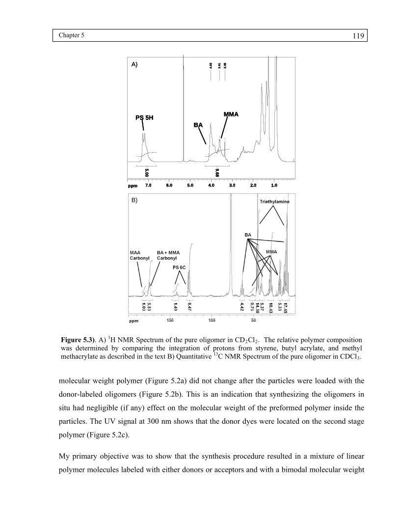
Chapter 5 119
ppm 1.02.03.04.05.06.07.0
4.0
3
3.6
1
3.3
5
5.00
9.68
PS 5HBA
MMA
A)
B)
ppm 1.02.03.04.05.06.07.0
4.0
3
3.6
1
3.3
5
5.00
9.68
PS 5HBA
MMA
ppm 1.02.03.04.05.06.07.0
4.0
3
3.6
1
3.3
5
5.00
9.68
PS 5HBA
MMA
A)
B)
Figure 5.3). A) 1H NMR Spectrum of the pure oligomer in CD2Cl2. The relative polymer composition was determined by comparing the integration of protons from styrene, butyl acrylate, and methyl methacrylate as described in the text B) Quantitative 13C NMR Spectrum of the pure oligomer in CDCl3.
molecular weight polymer (Figure 5.2a) did not change after the particles were loaded with the
donor-labeled oligomers (Figure 5.2b). This is an indication that synthesizing the oligomers in
situ had negligible (if any) effect on the molecular weight of the preformed polymer inside the
particles. The UV signal at 300 nm shows that the donor dyes were located on the second stage
polymer (Figure 5.2c).
My primary objective was to show that the synthesis procedure resulted in a mixture of linear
polymer molecules labeled with either donors or acceptors and with a bimodal molecular weight

Chapter 5 120
distribution. It is challenging to assign an accurate molecular weight to such a mixture of
polymer chains. Here, I took advantage of the chromophores attached to the chains and used the
more resolved UV spectra to assign molecular weights. Following this procedure, I calculated
M ≈ 41,000, PDI 2.5 for the acceptor-labeled polymer, a value close to what was obtained from
Figure 5.2a. For the donor-labeled oligomer, analyzing the donor UV spectrum resulted in M ≈
2,400, PDI 2.1. These values (M , PDI) are close to those obtained when the oligomer alone was
synthesized with the same recipe.
n
n
n
The composition of the oligomer was tested in several ways. In preliminary experiments,
samples of oligomer-only latex were synthesized by seeded emulsion polymerization using only
a small amount (ca. 6 wt %) of preformed seed latex. These samples could be analyzed for
composition (by 1H NMR and 13C NMR, Figure 5.3) and molecular weight (by GPC) without
interference from the high-M component. Figure 5.3A shows that the signal of MMA at 3.61
ppm overlaps the broader BA signals at 3.5 to 4.1 ppm; therefore, line-fitting was performed
using Mestrec software. Additionally, there is no signal which can be used to quantify the
methacrylic acid content. These two problems were solved by using quantitative 13C NMR
analysis instead. Figure 5.3B represents the 13C NMR spectra obtained on pure oligomer. The
composition was determined by comparing the integration of carbons from the four different
monomers. Butyl acrylate (BA) was quantified by the triplet at 64 ppm, representing the first
carbon of the butyl chain, methyl methacrylate (MMA) was quantified by the triplet at 18 ppm
representing a superposition of the signal from the second last carbon of the butyl chain in BA
and the methyl group in MMA. Styrene was quantified by the peaks at 127 and 144 ppm, in total
representing the 6 aromatic carbons. Methyacrylic acid (MAA) was quantified by the peak at 181
ppm, representing the carbonyl carbon of the deprotonated carboxylic acid. Other overlapped
peaks were not used in the analysis in order to limit the calculated standard errors.
In the two-component latex samples, the dialyzed dispersion was freeze dried and the polymer
composition was characterized by quantitative 1D 13C NMR. Initial spectra obtained on this
sample showed an overlap between carbonyl carbon of MAA and those of BA and MMA at 172-
177 ppm. Since MAA contributes a small fraction of the total polymer, line-fitting was not
preferred. Instead, MAA was neutralized by adding triethylamine to shift the MAA carbonyl
carbon to 181-182 ppm as shown in the inset of Figure 5.4. The polymer composition was
determined by comparing the integration of carbons from the four different monomers. Butyl

Chapter 5 121
Figure 5.4) Quantitative 13C NMR spectrum of the two-component polymer in CDCl3.
acrylate (BA) was quantified by the triplets at 64 ppm, representing the first carbon of the butyl
chain. Methyl methacrylate (MMA) was quantified by the triplet at 18 ppm, representing the
superposition of the signal from the second last carbon of the butyl chain in BA and the methyl
group in MMA. We preferred not to use the quartet at 51 ppm from PMMA, because it
represents two carbons, the -methyl group and the backbone CH2, which might have a slower
relaxation under the conditions of the experiment. Styrene was quantified by the peaks at 127
and 144 ppm, in total representing the 6 aromatic carbons. Methacrylic acid (MAA) was
quantified by the peak at 181 ppm, representing the carbonyl carbon of the deprotonated
carboxylic acid. Overlapped peaks were not used in the analysis in order to limit the calculated
standard errors. The results show that the final polymer contained mole fractions 0.47 ± 0.03 BA,
0.36 ± 0.02 MMA, 0.11 ± 0.01 Sty and 0.05 ± 0.01, MAA close to the amount targeted in the
reaction: 0.499 BA, 0.32 MMA, 0.08 Sty, 0.07 MAA.
Particle size and particle size distribution were measured by CHDF and DLS. As shown in
Figure 5.5, CHDF traces showed a single distribution of particle size. These traces showed that

Chapter 5 122
0
25
50
75
100
0 100 200 300 400 500 600Particle Size (nm)
No
rmal
ized
De
tect
or
Ou
tpu
t (m
AU
)Final particles
A-P(BA55MMA45) particles
0
25
50
75
100
0 100 200 300 400 500 600Particle Size (nm)
No
rmal
ized
De
tect
or
Ou
tpu
t (m
AU
)Final particles
A-P(BA55MMA45) particles
Figure 5.5) Capillary hydrodynamic fractionation fractograms for the parent particle (A-P(BA55MMA45)) and particles after being modified in situ with the oligomers (final particles). Both curves show that there is only one population of particles in the sample and the 2nd stage polymerization did not create new particles of donor-labeled oligomer.
the average particle radius of the A-P(BA-MMA) particles and the two-component particles were
ca. 51 and 63 nm respectively. These values are close to what was obtained by DLS as shown in
Table 5.2. Single particle size distributions obtained in CHDF traces confirms that secondary
nucleation was suppressed during the seeded reactions. The particles had narrow particles size
distributions as revealed by the CHDF traces and the light scattering measurements.
To synthesize the oligomers with carboxylic acid functionalities, I preferred using MAA to
acrylic acid (AA) because of the lower water solubility of MAA. To determine the incorporation
efficiency of MAA during the second seeded reaction, I carried out potentiometric titration
experiments in an organic solvent (THF). The titration curve is plotted in Figure 5.6. In this
figure, the initial rapid rise in pH suggests the presence of strong acid groups in the sample.
These groups are likely the sulfate groups from the initiator that could not be removed by
dialysis. The highlighted area in Figure 5.6 corresponds to 8.05 10-2 mmol base, which is
slightly higher than the amount of COOH groups in the polymer (7.62 10-2 mmol) predicted
from the monomer feed. The onset and the end point of the titration were determined from the
inflection points in the potentiometric curve using a derivative plot. During the titration 30-50 µL
aliquots of base were added to the solution. As shown in Figure 5.6, the onset point occurred
when ca. 160 µL of 0.05 N was added to the solution. This volume is comparable to the volume
of the aliquots added at each step and thus there is a high uncertainty in the starting point of the
1
3
5
7
9
11
15
0 5 100 1500 200 2
-0.01
0.01
0.03
0.05
0.07
0.09
0.13
pH
Na(OH) 0.05
/ d
(vo
l.)
13
00 0 0 500
0.11
N vol. μL
d(p
H)
1
3
5
7
9
11
15
0 5 100 1500 200 2
-0.01
0.01
0.03
0.05
0.07
0.09
0.13
pH
Na(OH) 0.05
/ d
(vo
l.)
13
00 0 0 500
0.11
N vol. μL
d(p
H)
Figure 5.6) Potentiometric titration curve of the two-component particles dissolved in THF. The onset and the end point of the titration are determined from the maxima of the derivative plot. The highlighted area corresponds to 80.5 µmol NaOH.

Chapter 5 123
titration using this concentration of base. Using a more dilute (0.025N) NaOH solution caused
polymer precipitation. Nevertheless, the difference (5.6 %) between the experimentally measured
value and the calculated value is relatively small. The most meaningful interpretation of this
result is that all of the methacrylic acid in the recipe was incorporated into the polymer.
Table 5.2. Characterization of the nanoparticle dispersions used in this study
Sample Mn a Mw/Mn Tg (°C) b Rh (nm) c poly. d Solids Content wt %
A-P(BA55MMA45) e 41,000 2.5 6.8 55 0.038 38.5
A-P(BA55MMA45)+D-oligomer e,f — — -4.1 68 0.075 39.2
A-P(BA55MMA45) e 43,400 2.8 7.4 54 0.025 38.4
A-P(BA55MMA45) + oligomer e,f — — -3.8 70 0.052 40.1
D-P(BA55MMA45) e 47,400 3.1 7.2 60 0.037 37.3
D-P(BA55MMA45) + oligomer — — -4.1 70 0.032 40.1
oligomer 2,800 2.4 -24.1 58 0.083 34.1
a. Nominal molecular weights obtained by gel permeation chromatography by reference to polystyrene standards (Fig 5.1). Composition was determined by 1H and 13C NMR (Figs 5.2, 5.3).
b. Glass transition temperatures taken as the mid point of the deflection in differential scanning calorimetry measurements.
c. For as prepared samples after purification by dialysis. For oligomer-containing samples, the acid groups in the oligomer are in their protonated state.
d. Particle size distribution measured from second cumulant analysis. The absence of small particles in the sample from possible secondary nucleation was monitored by capillary hydrodynamic fractionation chromatography (CHDF, Fig 5.4)
e. D- and A- refer, respectively, to polymers labeled with donor dye (1 mol %) and acceptor dye. When the oligomer was donor-labeled, the high-M polymer contained 0.3 mol% acceptor dye. When the oligomer was not labeled, the high-M acceptor-labeled polymer contained 0.6mol% dye.
f. The oligomer composition was BA (51.2 mol %), MMA (11.8 mol %), styrene (17.2 mol %), methacrylic acid (MAA, 13.9 mol %), C12-SH (5.9 mol %). The two-component nanoparticles contain a 1:1 weight ratio of high-M polymer and oligomer.
The surface acid groups of the two-component particles were determined by acid-base back
titration of the dispersion in water. Back titration was preferred since previous experiments
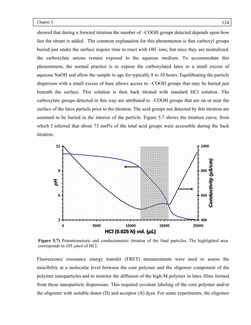
Chapter 5 124
showed that during a forward titration the number of –COOH groups detected depends upon how
fast the titrant is added. The common explanation for this phenomenon is that carboxyl groups
buried just under the surface require time to react with OH ions, but once they are neutralized,
the carboxylate anions remain exposed to the aqueous medium. To accommodate this
phenomenon, the normal practice is to expose the carboxylated latex to a small excess of
aqueous NaOH and allow the sample to age for typically 8 to 10 hours. Equilibrating the particle
dispersion with a small excess of base allows access to –COOH groups that may be buried just
beneath the surface. This solution is then back titrated with standard HCl solution. The
carboxylate groups detected in this way are attributed to –COOH groups that are on or near the
surface of the latex particle prior to the titration. The acid groups not detected by this titration are
assumed to be buried in the interior of the particle. Figure 5.7 shows the titration curve, from
which I inferred that about 73 mol% of the total acid groups were accessible during the back
titration.
-
3
6
9
12
0 5000 10000 15000 20000
400
600
800
1000
HCl (0.025 N) vol. (μL)
pH
Co
nd
uct
ivit
y (μ
S/c
m)
3
6
9
12
0 5000 10000 15000 20000
400
600
800
1000
HCl (0.025 N) vol. (μL)
pH
Co
nd
uct
ivit
y (μ
S/c
m)
3
6
9
12
0 5000 10000 15000 20000
400
600
800
1000
3
6
9
12
0 5000 10000 15000 20000
400
600
800
1000
HCl (0.025 N) vol. (μL)
pH
Co
nd
uct
ivit
y (μ
S/c
m)
Figure 5.7) Potentiometeric and conductometric titration of the final particles. The highlighted area corresponds to 105 µmol of HCl.
Fluorescence resonance energy transfer (FRET) measurements were used to assess the
miscibility at a molecular level between the core polymer and the oligomer component of the
polymer nanoparticles and to monitor the diffusion of the high-M polymer in latex films formed
from these nanoparticle dispersions. This required covalent labeling of the core polymer and/or
the oligomer with suitable donor (D) and acceptor (A) dyes. For some experiments, the oligomer

Chapter 5 125
was labeled with phenanthrene as the donor dye (D-oligo), and the core polymer A-
P(BA55MMA45) was labeled with an N,N-dimethylaminobenzophenone derivative (NBen) as the
acceptor dye. For polymer diffusion experiments in latex films, parallel samples were prepared
with the high-M polymer labeled either with wither Phe or NBen, and the oligomer was left
unlabeled. The characteristics of these polymer nanoparticles are presented in Table 5.2. The
recipes used for the syntheses of these samples are collected in Table 5.1. The overall carboxylic
acid content was determined by titration in tetrahydrofuran (Figure 5.6). The results showed
complete incorporation of MAA into the oligomer.
5.3.1 Morphology transformation caused by a change in pH
For FRET studies of the morphology in the two-component polymer nanoparticles, the high-M
polymer was labeled with the acceptor dye and the oligomer was labeled with the donor dye (c.f.,
Table 5.1). The particles contained an equal weight of each component. FRET experiments were
performed on dilute dispersions of nanoparticles. 19 These measurements were carried out by
exciting the donor dye at 294 nm with a nanosecond pulsed diode and measuring its decay
profiles by the single-photon timing technique. 20 In a model latex containing a phenanthrene-
labeled oligomer but no dye in the core, the donor fluorescence decay was exponential, with a
lifetime D = 43.4 ns, irrespective of the solution pH. In the as-prepared two-component
particles, synthesized in the absence of added base, the carboxylic acid groups were primarily in
the protonated form. To study the effect of pH on the particle morphology, highly diluted
deionized dispersions (ca. 10-3 wt % solids) were added to aqueous solutions of NaOH or HCl
with the desired pH.
For the initial measurements, a trace of HCl was added to the nanoparticle solution to reduce the
pH to 3.0. The donor fluorescent decay curve (ID(t)) for this dispersion is shown as the lower
curve in Figure 5.8A. Adding NaOH to the dispersion to increase the pH to 11.0 led to an
immediate (minutes) and stable change in the ID(t) decay profile, presented as the upper curve in
Figure 5.8A. The slower but non-exponential donor decay rate for the sample at pH 11 indicates
that some energy transfer took place in the particles at pH 11, but much less than in the particles
at pH 3.
Corresponding measurements were carried out at a series of pH values between 3 and 11. These
decays were analyzed using the model-free approach presented in section 2.6, Chapter 2. Figure

Chapter 5 126
5.9A illustrates the variation of ΦET with pH for a dilute (10-3 wt %) aqueous dispersion of the
two-component latex particles. As one can observe, ΦET values are almost constant for particles
in acidic solutions but decrease when the pH of the dispersion was increased from 7 to 11. The
inflection point in the ΦET vs pH curve occurs between pH 8 and 9; a considerably higher value
compared to the literature values of the apparent pKa (4.7) of poly(methacrylic acid). 21,22 These
ΦET values are replotted in terms of the degree of neutralization of the carboxylic acid groups
in Figure 5.9B. Here one can see that the morphology transition occurs when more than 60% of
the titratable carboxylic acid groups were neutralized.
The high pKa value of the carboxylic acid units along the backbone of the oligomers points to the
reduced acidity of these groups and is probably due to the hydrophobicity of their environment in
the particles. Khokhlov et al. proposed a similar mechanism to explain the pH dependency of the
swelling behavior for hydrophobically modified carboxylated hydrogels. 23
At pH 3.0, ΦET = 0.51, which suggests a significant mixing between the two-components inside
the composite particle. At pH 11.0 the value of ΦET decreased to 0.22. As shown in Figure 5.10,
these changes were reversible. Addition of HCl to reduce the pH to 3 led to an increase in ΦET,
whereas subsequent addition of NaOH to raise the pH back to 11 resulted in a decrease in energy
transfer. While the changes in ΦET were fully reversible, each neutralization-protonation step
increased the ionic strength of the medium, and eventually the nanoparticles precipitated.
A)
B)
A)
B)
Figure 5.8) A) Phe fluorescence decay profiles of the two-component particles at pH 3.0 and 11.0; the uppermost curve is the exponential unquenched donor decay for a sample with no acceptor dye. Förster equation (eq 2.14) was used to fit the decay of the dispersion at pH 3.0 and Förster mixing (eq 2.16) was used for the decay at pH 11.0. B) Fit residuals for the decays presented in A. For the decay at pH 3.0, χ2 = 1.17 and for that at pH 11.0, χ2 = 1.08. In both cases, the residuals are randomly and evenly spaced around zero.

Chapter 5 127
The reversibility of the changes in ΦET (Figure 5.10) provides strong evidence that, at high pH,
where the carboxyl groups are fully neutralized, the oligomer remained part of the nanoparticle
structure. Preliminary experiments with a more hydrophilic oligomer lacking styrene units gave
different results: a similar ΦET value for the initial sample at low pH, but incomplete reversibility
on successive additions of acid and then base. After centrifugation of this sample at high pH, I
observed by UV-Vis spectroscopy the presence of soluble donor-labeled materials in the
supernatant that I attribute to water-soluble oligomer. I present more details about these
experiments in Appendix (II). For the nanoparticles loaded with the styrene-containing oligomer,
almost no water-soluble oligomer could be detected following centrifugation of a latex sample at
high pH.
0.2
0.3
0.4
0.5
0.6
1 3 5 7 9 11 13
0.2
0.3
0.4
0.5
0.6
0 0.2 0.4 0.6 0.8 1
pH
α
ΦE
TΦ
ET
A)
B)
0.2
0.3
0.4
0.5
0.6
1 3 5 7 9 11 13
0.2
0.3
0.4
0.5
0.6
0 0.2 0.4 0.6 0.8 1
pH
α
ΦE
TΦ
ET
A)
B)
Figure 5.9) A) Variation of the quantum efficiency of energy transfer (ΦET) as a function of pH for highly diluted dispersions. B) Variation of ΦET as a function of ionization degree (α) from data presented in (A). Values of α were calculated from the titration curve in Figure 5.7.

Chapter 5 128
3 11 3 11 3
pH
Φ0.2
0.3
0.4
0.5
0.6
3 11 3 11 3pH
ET
3 11 3 11 3
pH
Φ0.2
0.3
0.4
0.5
0.6
3 11 3 11 3pH
ET
Figure 5.10) Variation of the quantum efficiency of energy transfer (ΦET) when pH was switched back and forth between acidic and alkaline conditions. The results show that the transition is reversible.
0
0.2
0.4
0.6
0.8
1
1.2
0.0001 0.01 1 100 10000
0
0.2
0.4
0.6
0.8
1
1.2
10 100 1000
[G2(τ
)-A
] /
A
τ (ms)
Rh (nm)
f(R
h)
pH 11
pH 3
pH 11pH 3
a)
b)
0
0.2
0.4
0.6
0.8
1
1.2
0.0001 0.01 1 100 10000
0
0.2
0.4
0.6
0.8
1
1.2
10 100 1000
[G2(τ
)-A
] /
A
τ (ms)
Rh (nm)
f(R
h)
0
0.2
0.4
0.6
0.8
1
1.2
10 100 1000
[G2(τ
)-A
] /
A
τ (ms)
Rh (nm)
f(R
h)
pH 11
pH 3
pH 11pH 3
a)
b)
Figure 5.11) Normalized autocorrelation functions (a) and CONTIN plots (b) from DLS measurements on particles at pH 3 and 11. From a cumulant analysis, we find that Rh increases from 68 nm at pH 3 to 78 nm at pH 11, accompanied by an increase in polydispersity (0.075 at pH 3; 0.117 at pH 11).
Figure 5.11A presents the normalized autocorrelation functions measured by dynamic light
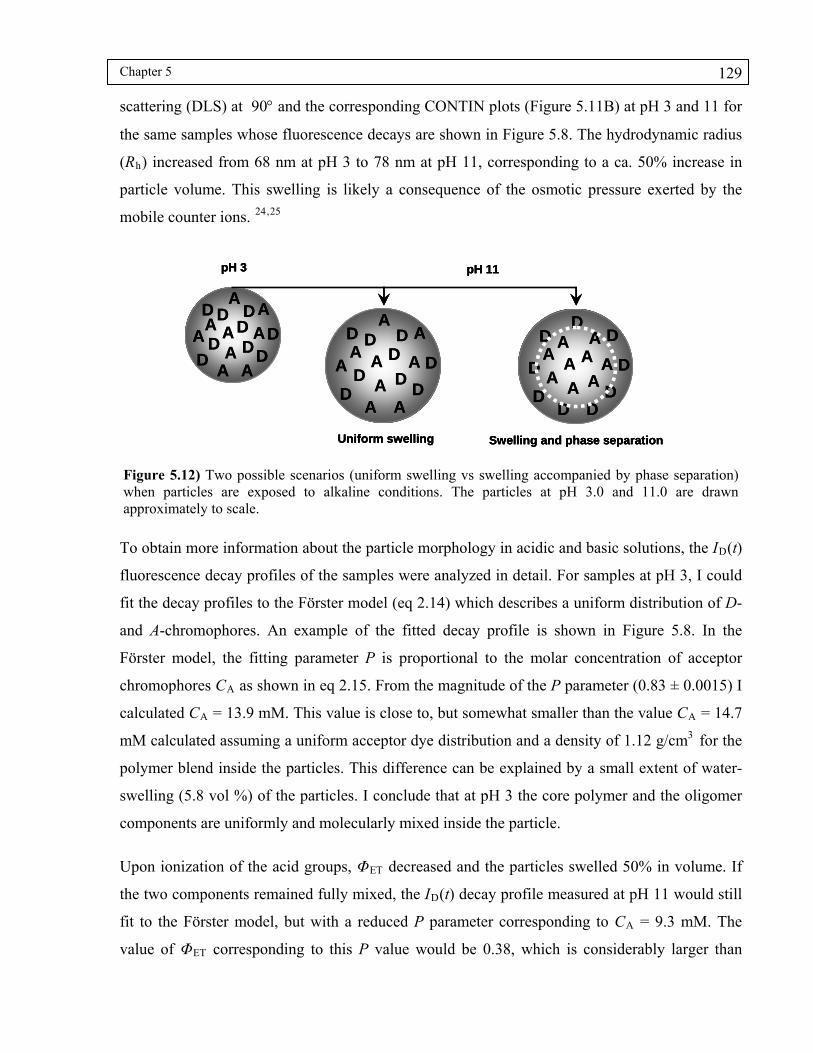
Chapter 5 129
scattering (DLS) at 90 and the corresponding CONTIN plots (Figure 5.11B) at pH 3 and 11 for
the same samples whose fluorescence decays are shown in Figure 5.8. The hydrodynamic radius
(Rh) increased from 68 nm at pH 3 to 78 nm at pH 11, corresponding to a ca. 50% increase in
particle volume. This swelling is likely a consequence of the osmotic pressure exerted by the
mobile counter ions. 24,25
A
D
D
AD
DD
DA
A
AD
D
A
AA
DA
A
D
D
AD
DD
DA
A
A
D
D
A
A
A
DA
D
A
A
DD
DA
AA
D
D
D
D
D
A
A
AA
pH 3 pH 11
Uniform swelling Swelling and phase separation
A
D
D
AD
DD
DA
A
AD
D
A
AA
DA
A
D
D
AD
DD
DA
A
A
D
D
A
A
A
DA
D
A
A
DD
DA
AA
D
D
D
D
D
A
A
AA
pH 3 pH 11
Uniform swelling Swelling and phase separation
A
D
D
AD
DD
DA
A
AD
D
A
AA
DA
A
D
D
AD
DD
DA
A
AD
D
A
AA
DA
A
D
D
AD
DD
DA
A
AD
D
A
AA
DA
A
D
D
AD
DD
DA
A
A
D
D
A
A
A
DA
A
D
D
AD
DD
DA
A
A
D
D
A
A
A
DA
A
D
D
AD
DD
DA
A
A
D
D
A
A
A
DA
D
A
A
DD
DA
AA
D
D
D
D
D
A
A
AA
D
A
A
DD
DA
AA
D
D
D
D
D
A
A
AA
D
A
A
DD
DA
AA
D
D
D
D
D
A
A
AA
pH 3 pH 11
Uniform swelling Swelling and phase separation
Figure 5.12) Two possible scenarios (uniform swelling vs swelling accompanied by phase separation) when particles are exposed to alkaline conditions. The particles at pH 3.0 and 11.0 are drawn approximately to scale.
To obtain more information about the particle morphology in acidic and basic solutions, the ID(t)
fluorescence decay profiles of the samples were analyzed in detail. For samples at pH 3, I could
fit the decay profiles to the Förster model (eq 2.14) which describes a uniform distribution of D-
and A-chromophores. An example of the fitted decay profile is shown in Figure 5.8. In the
Förster model, the fitting parameter P is proportional to the molar concentration of acceptor
chromophores CA as shown in eq 2.15. From the magnitude of the P parameter (0.83 ± 0.0015) I
calculated CA = 13.9 mM. This value is close to, but somewhat smaller than the value CA = 14.7
mM calculated assuming a uniform acceptor dye distribution and a density of 1.12 g/cm3 for the
polymer blend inside the particles. This difference can be explained by a small extent of water-
swelling (5.8 vol %) of the particles. I conclude that at pH 3 the core polymer and the oligomer
components are uniformly and molecularly mixed inside the particle.
Upon ionization of the acid groups, ΦET decreased and the particles swelled 50% in volume. If
the two components remained fully mixed, the ID(t) decay profile measured at pH 11 would still
fit to the Förster model, but with a reduced P parameter corresponding to CA = 9.3 mM. The
value of ΦET corresponding to this P value would be 0.38, which is considerably larger than

Chapter 5 130
experimentally obtained value at pH 11 (0.22). Moreover, attempts to fit the decay profiles
obtained at pH 11 to the Förster model resulted in poor fit with noticeably large, nonrandom
residuals in the early channels. Therefore, the idea of uniform swelling at pH 11 cannot explain
the donor fluorescence decay profile (Figure 5.12), and the low extent of energy transfer points
instead to microphase separation. I attributed the observed changes in ΦET to a reversible
morphology transition from a mixed state (at pH 3.0) to a charge-induced microphase separation
(at pH 11.0). In other words, a reversible rearrangement of the components occurred as a
consequence of deprotonation of COOH groups, which led to a phase rich in the ionized donor-
labeled oligomers that could remix with the acceptor-labeled polymer when the pH was
decreased.
While the FRET experiments provide unambiguous evidence for phase separation, these
experiments by themselves do not establish a core-shell type morphology for the composite
particles. The characteristic length scale sampled in a FRET experiment (on the order of 5Ro) is
sensitive to microphase separation but is too small to distinguish core-shell from other occlusion
types of phase separation. To obtain additional information, I took particles equilibrated at pH 11
and titrated them with acid. Here I found that 74% of the –COOH groups introduced in the
oligomer synthesis could be titrated as shown in Figure 5.7. I infer from this result that the phase
separation at high pH brought most of the acid groups close enough to the surface to be
titrated.26 This suggests the formation of a core-shell structure at alkaline pH. This morphology
transition is delineated schematically in Figure 5.12.
I made several attempts to obtain TEM images that would allow visualization of the polymer
nanoparticles morphology. None of these experiments were informative. These included attempts
to stain the particles with uranyl acetate or cesium hydroxide prior to or after casting samples
onto TEM grids. Unfortunately, the particles studied here are extremely soft at room
temperature, and it is difficult to keep them intact when preparing the TEM grids. In addition,
these polymers appeared to be very sensitive to damage when exposed to the electron beam.
Attempts to use a cryo-holder to image samples at -120 °C for grids prepared at room
temperature showed only fused pancake-like structures.

Chapter 5 131
Taking the core-shell structure as a model, I carried out a more detailed analysis of the ID(t)
decay profiles measured at pH 11 to determine the nature of the interface between the
hydrophobic polymer core and the carboxylate-rich oligomer shell. This analysis assumes that, as
in traditional polymer blends, the concentration profile across the interface between the
components can be described by the Helfand-Tagami (HT) model, 27 and the donor and acceptor
profiles across the interface follows the segment density profile of the components. I carried out
simulations to calculate theoretical ID(t) profiles based upon a Monte-Carlo sampling technique
assuming various values of the interface thickness δ. The details of these calculations are
presented in section 2.8, Chapter 2. These theoretical profiles were convoluted with the
instrument response function obtained in the experiments. The value of δ was then optimized to
get the best fit of experimental and theoretical decay profiles.
Fit
Res
idu
als
Time (ns)
Inte
nsi
ty (
cou
nts
)
a)
pH 11.0
Lamp
Oligomer
Time (ns)
P(BA55MMA45)Cn
χ2
δ (nm)
r (nm)
b)
c)
d)
0
1
0 20 40 60 80
0.9
1.5
2.1
2.7
10 15 20 25 30 35
1
10
102
103
104
105
0 50 100 150 200 250
-3-113
0 50 100 150 200 250Fit
Res
idu
als
Time (ns)
Inte
nsi
ty (
cou
nts
)
a)
pH 11.0
Lamp
Oligomer
Time (ns)
P(BA55MMA45)Cn
χ2
δ (nm)
r (nm)
b)
c)
d)
0
1
0 20 40 60 80
0.9
1.5
2.1
2.7
10 15 20 25 30 35
1
10
102
103
104
105
0 50 100 150 200 250
-3-113
0 50 100 150 200 250
Figure 5.13) a) Phe fluorescence decay of the composite particles at pH 11.0 fitted to a simulated decay obtained based on HT model concentration profile at δ=21±1 nm, b) Weighted residuals of the fit presented in (a), c) plot of χ2 obtained when decays based on various δ were fitted to the experimental decay at pH 11.0, d) plot of normalized radial concentration profile inside composite particle, the solid line represents the high molecular weight component and the dashed line represents the oligomer concentration.
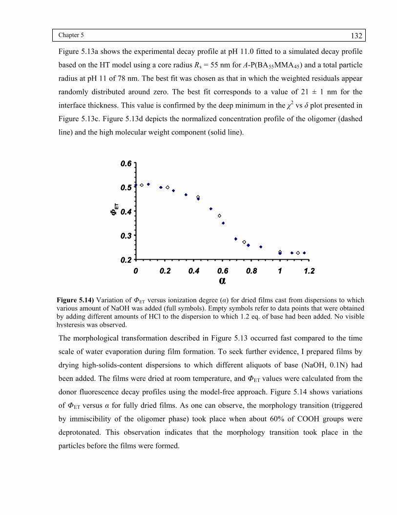
Chapter 5 132
Figure 5.13a shows the experimental decay profile at pH 11.0 fitted to a simulated decay profile
based on the HT model using a core radius Rs = 55 nm for A-P(BA55MMA45) and a total particle
radius at pH 11 of 78 nm. The best fit was chosen as that in which the weighted residuals appear
randomly distributed around zero. The best fit corresponds to a value of 21 ± 1 nm for the
interface thickness. This value is confirmed by the deep minimum in the χ2 vs δ plot presented in
Figure 5.13c. Figure 5.13d depicts the normalized concentration profile of the oligomer (dashed
line) and the high molecular weight component (solid line).
0.2
0.3
0.4
0.5
0.6
0 0.2 0.4 0.6 0.8 1 1.2
ΦE
T
α
0.2
0.3
0.4
0.5
0.6
0 0.2 0.4 0.6 0.8 1 1.2
ΦE
T
α
Figure 5.14) Variation of ΦET versus ionization degree (α) for dried films cast from dispersions to which various amount of NaOH was added (full symbols). Empty symbols refer to data points that were obtained by adding different amounts of HCl to the dispersion to which 1.2 eq. of base had been added. No visible hysteresis was observed.
The morphological transformation described in Figure 5.13 occurred fast compared to the time
scale of water evaporation during film formation. To seek further evidence, I prepared films by
drying high-solids-content dispersions to which different aliquots of base (NaOH, 0.1N) had
been added. The films were dried at room temperature, and ΦET values were calculated from the
donor fluorescence decay profiles using the model-free approach. Figure 5.14 shows variations
of ΦET versus α for fully dried films. As one can observe, the morphology transition (triggered
by immiscibility of the oligomer phase) took place when about 60% of COOH groups were
deprotonated. This observation indicates that the morphology transition took place in the
particles before the films were formed.

Chapter 5 133
As an additional test of the reversibility of the morphology transition, I added various aliquots of
HCl (0.1 N) to the high-solids dispersion to which 1.2 eq NaOH had been added and used these
dispersions to prepare films (empty symbols in Figure 5.14). The ΦET values increased for films
formed in this way. I conclude that the oligomer became increasingly miscible with the high
molecular weigh polymer as its carboxylate groups were protonated. No hysteresis was observed
in this experiment.
The high-solids dispersion maintained its colloidal stability even when exposed to high
concentrations of base. When a high solids dispersion of particles synthesized with styrene-free
oligomer was exposed to excess base, the dispersion thickened. This increase in viscosity is
consistent with the idea that protonated styrene-free oligomer dissolves at high pH.
Upon adding 0.45 eq HCl to the high-solids dispersion to which 1.2 eq NaOH had been added, a
change in turbidity of the dispersion was observed. Also, there was some indication of an
increase in particle size by dynamic light scattering. These observations are signs of the onset of
particle flocculation. The dispersion tended to aggregate more severely when higher amounts of
HCl were added.
5.3.2 Promotion of polymer diffusion by the acid-rich oligomer
To test the ability of oligomer to enhance the diffusion rate of the high-M latex polymer, I
needed polymer samples similar to those described above but labeled differently with donor and
acceptor dyes. Since here, I was interested in the rate of interdiffusion of high molecular weight
polymer between adjacent cells formed from latex nanoparticles upon drying, it was the high-M
component that needed to be labeled. This requires a pair of essentially identical two-component
latex nanoparticle samples, one with the high-M component labeled with Phe as the donor dye
and one with the high-M component labeled with NBen as the acceptor dye. Both samples
should contain 50 wt % unlabeled oligomer. For comparison purposes, I prepared a pair of latex
samples consisting of D- and A-labeled high-M polymer with no oligomer content. This sample
was used to determine the polymer diffusion rate in the absence of added oligomer.
I synthesized D-P(BA55MMA45), labeled with 1 mol % Phe, and A-P(BA55MMA45), labeled
with 0.6 mol% NBen. These samples were then used to synthesize two-component latex
nanoparticles containing 50 wt % unlabeled oligomer. The high-M D-P(BA55MMA45) sample
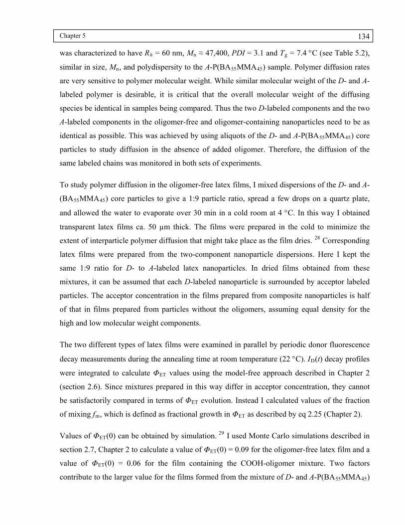
Chapter 5 134
was characterized to have Rh = 60 nm, Mn ≈ 47,400, PDI = 3.1 and Tg = 7.4 C (see Table 5.2),
similar in size, Mn, and polydispersity to the A-P(BA55MMA45) sample. Polymer diffusion rates
are very sensitive to polymer molecular weight. While similar molecular weight of the D- and A-
labeled polymer is desirable, it is critical that the overall molecular weight of the diffusing
species be identical in samples being compared. Thus the two D-labeled components and the two
A-labeled components in the oligomer-free and oligomer-containing nanoparticles need to be as
identical as possible. This was achieved by using aliquots of the D- and A-P(BA55MMA45) core
particles to study diffusion in the absence of added oligomer. Therefore, the diffusion of the
same labeled chains was monitored in both sets of experiments.
To study polymer diffusion in the oligomer-free latex films, I mixed dispersions of the D- and A-
(BA55MMA45) core particles to give a 1:9 particle ratio, spread a few drops on a quartz plate,
and allowed the water to evaporate over 30 min in a cold room at 4 C. In this way I obtained
transparent latex films ca. 50 µm thick. The films were prepared in the cold to minimize the
extent of interparticle polymer diffusion that might take place as the film dries. 28 Corresponding
latex films were prepared from the two-component nanoparticle dispersions. Here I kept the
same 1:9 ratio for D- to A-labeled latex nanoparticles. In dried films obtained from these
mixtures, it can be assumed that each D-labeled nanoparticle is surrounded by acceptor labeled
particles. The acceptor concentration in the films prepared from composite nanoparticles is half
of that in films prepared from particles without the oligomers, assuming equal density for the
high and low molecular weight components.
The two different types of latex films were examined in parallel by periodic donor fluorescence
decay measurements during the annealing time at room temperature (22 C). ID(t) decay profiles
were integrated to calculate ΦET values using the model-free approach described in Chapter 2
(section 2.6). Since mixtures prepared in this way differ in acceptor concentration, they cannot
be satisfactorily compared in terms of ΦET evolution. Instead I calculated values of the fraction
of mixing fm, which is defined as fractional growth in ΦET as described by eq 2.25 (Chapter 2).
Values of ΦET(0) can be obtained by simulation. 29 I used Monte Carlo simulations described in
section 2.7, Chapter 2 to calculate a value of ΦET(0) = 0.09 for the oligomer-free latex film and a
value of ΦET(0) = 0.06 for the film containing the COOH-oligomer mixture. Two factors
contribute to the larger value for the films formed from the mixture of D- and A-P(BA55MMA45)

Chapter 5 135
polymer nanoparticles. First, there is a higher concentration of A-groups (CA) in the A-labeled
phase. Second, there is a greater interfacial area in films formed by these smaller particles.
Experimental values of ΦET in newly formed films can be larger than these values if some
polymer interdiffusion occurs as the wet films dry on the substrate. In Figure 5.15, the extent of
polymer diffusion that took place during film preparation is indicated by values of fm(t=0) > 0.
ΦET(∞) refers to the final value of the energy transfer quantum efficiency following complete
mixing of donors and acceptors. To determine this value, I prepared fully mixed films by solvent
casting: A dried latex film was dissolved in a small amount of tetrahydrofuran (THF). The
solvent was allowed to evaporate, and the films were annealed at 70°C in an oven overnight to
remove traces of THF. From fluorescence decay measurements on these films I obtained ΦET(∞)
= 0.83 for the oligomer-free mixture and ΦET(∞) = 0.70 for the two-component polymer mixture.
The mixture with no oligomer has a higher value of ΦET(∞) because of the higher CA in this
film. These experimental values are close to those obtained from simulations, i.e. 0.87 for the
oligomer-free mixture and 0.71 for COOH-oligomer mixture.
In Figure 5.15, I compare the evolution of mixing due to polymer diffusion across the
interparticle boundaries in the two sets of latex films. The differences are striking. For the
oligomer-free film, polymer diffusion at room temperature occurred on a time scale of tens of
hours, reaching fm = 0.5 after about 2000 min. In contrast, in the presence of what is admittedly a
large amount of COOH-oligomer, polymer diffusion took place on the time scale of minutes
(c.f., the inset in Figure 5.15), reaching fm = 0.5 after about 10 min. Figure 5.16 represents the
values of calculated apparent diffusion coefficients Dapp as a function of the extent of mixing.
Here Dapp values are calculated according to the procedure described in section 2.6.2 of Chapter
2. These calculations indicate that the presence of the oligomer in the mixture of D- and A-
P(BA55MMA45) polymer increased the Dapp values by two orders of magnitude.
In Figure 5.16, the values of Dapp calculated for the sample to which 1 eq NaOH was added are
lower than for the sample that contained the acid form of the oligomer. Dapp values for the
sample in which oligomers were neutralized with ammonia are in between these two curves.
Neutralized oligomer had limited miscibility with the high molecular weight polymer as
demonstrated in Figure 5.13. As described in Chapter 3 of this thesis, plasticization only occurs
when plasticizer (in this case the oligomer) and polymer are miscible at the molecular level.
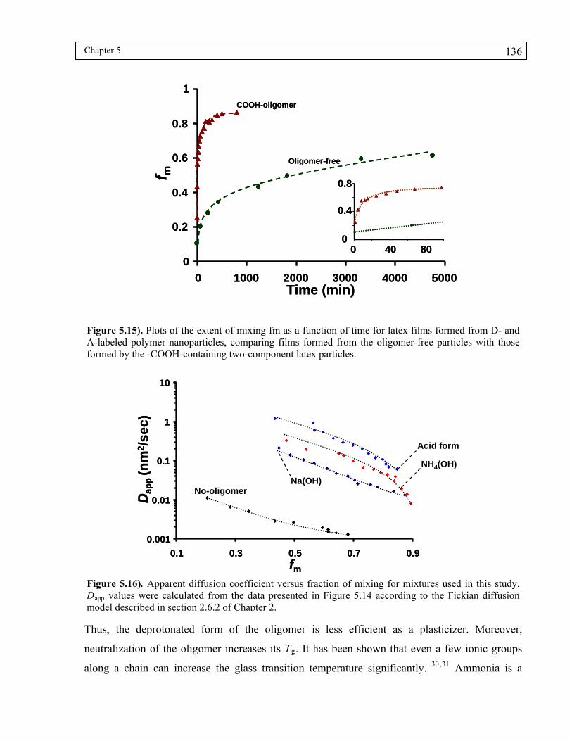
Chapter 5 136
0
0.2
0.4
0.6
0.8
1
0 1000 2000 3000 4000 5000
0
0.4
0.8
0 40 80
Oligomer-free
COOH-oligomer
Time (min)
f m
0
0.2
0.4
0.6
0.8
1
0 1000 2000 3000 4000 5000
0
0.4
0.8
0 40 80
Oligomer-free
COOH-oligomer
Time (min)
f m
Figure 5.15). Plots of the extent of mixing fm as a function of time for latex films formed from D- and A-labeled polymer nanoparticles, comparing films formed from the oligomer-free particles with those formed by the -COOH-containing two-component latex particles.
0.001
0.01
0.1
1
10
0.1 0.3 0.5 0.7 0.9fm
Da
pp
(nm
2 /se
c)
0.001
0.01
0.1
1
10
0.1 0.3 0.5 0.7 0.9fm
Da
pp
(nm
2 /se
c)
No-oligomer
Acid form
NH4(OH)
Na(OH)
Figure 5.16). Apparent diffusion coefficient versus fraction of mixing for mixtures used in this study. Dapp values were calculated from the data presented in Figure 5.14 according to the Fickian diffusion model described in section 2.6.2 of Chapter 2.
Thus, the deprotonated form of the oligomer is less efficient as a plasticizer. Moreover,
neutralization of the oligomer increases its Tg. It has been shown that even a few ionic groups
along a chain can increase the glass transition temperature significantly. 30,31 Ammonia is a

Chapter 5 137
volatile (soft) base. The sample which was neutralized with ammonia showed higher Dapp values
than the sample to which NaOH was added. This observation suggests that as this sample was
aged, ammonia evaporated and left the acid form of the oligomer which could plasticize the
diffusion. The Dapp values are cumulative averages of diffusion coefficients of species that have
diffused up to a certain time. Therefore, even though at long aging times most of the ammonia
may have left the film, Dapp values for this film were still lower that those values obtained for the
unneutralized film.
5.3.3 Retarded coalescence: the early stage of film formation at acidic and basic pH
In this section, I examine the consequences of changing pH on the earliest stages of film
formation for the two-component latex films. For these experiments, I took advantage of a wet
sample accessory developed in our laboratory that allows measurement of fluorescence decay
profiles through a low-resolution microscope, with sub-millimeter resolution, on partially dry
latex films. The instrumental setup is described elsewhere.32 For these experiments, ca. 100 μL
of individual mixtures of D- and A-labeled latex nanoparticles were each cast onto a 25 mm
diameter quartz disk and allowed to dry at 22°C and 35% relative humidity (RH). The
dispersions dried from the edges inward with the formation of a distinct drying front that
separated the transparent dry film from the cloudy center. I used digital photographs to image the
drying process. Figure 5.17 represents images of the four types of partially dried latex films
examined, each allowed to dry for ca. 100 min. As a reference, Figure 5.17a shows a film of the
oligomer-free dispersion consisting of a mixture of D- and A-P(BA55MMA45) particles in a 1:9
ratio. The other images are of films of the two-component latex, in b) with the oligomer in the –
COOH form, and in c) and d), neutralized with one equivalent of NH4OH and NaOH,
respectively.
These images show that a translucent halo followed by a turbid ring separated the wet spot from
the transparent dry polymer film for both the oligomer-free latex film (Figure 5.17a) and for the
two-component latex in the –COOH form (Figure 5.17b). This turbid ring appeared after ca. 5
min of drying and advanced concentrically with the drying front as the wet spot contracted. This
ring is likely to be a signature of the compaction front identified by Scriven and coworkers.33 At
the compaction front, water has receded from the partially deformed latex particles, creating air
voids, which strongly scatter the incident light. As the film continues to dry, this foam-like

Chapter 5 138
structure collapses into a void-free film. In films neutralized with base, no compaction front can
be seen (Figure 5.17c and 5.17d). There was a single boundary (the drying front) between the dry
edge and the turbid spot. This boundary formed early on in the drying process and receded
inward during drying.
Figure 5.17). Partially dried latex films containing a mixture of D- and A-labeled polymer nanoparticles after 100 min at 22 °C and 35% RH. a) Oligomer-free latex; b) Two-component latex particles containing the COOH oligomer, c) Two-component latex to which 1 eq NH4(OH) was added to the dispersion; d) Two-component latex to which 1 eq NaOH was added to the dispersion. Fluorescence decay measurements were carried out along the dashed line from the edge of the quartz disk, across the drying front and into the wet (turbid) dispersion.
After ca. 100 min drying, each film was immediately transferred to a hermetically sealed
chamber precooled to 5 C to stop the drying and to suppress further polymer diffusion. Then
donor fluorescence decay measurements were carried out at a series of positions (along the white
dotted lines in each image) from the edge of the disk, across the drying front, and into the turbid
wet region of the dispersion. ID(t) profiles were analyzed using the model-free approach
presented in section 2.6, Chapter 2 and the fm values were calculated using eq 2.25. These values
are plotted as a function of the distance from the drying front in Figure 5.18. In Figure 5.18a and
b, the bold dashed vertical lines refer to the compaction front, the inner edge of the bright corona
surrounding the wet spot in the middle of the film, and the drying front is chosen as the outer
edge of this bright ring, which Scriven has called the coalescence front. The idea behind this
term is that coalescence refers to the step in which all hydrophilic material is squeezed out of the

Chapter 5 139
interstitial spaces between adjacent cells in a latex film 34 and the polymers in these cells come
into contact. Diffusion across a polymer-polymer boundary takes place only after polymer
molecules at each side of the boundary come into close contact, a situation described as ‘wetting’
by Wool. 35
Distance from the drying front
f m
Wet Spot
a)
0.05
0.15
0.25
0.35
0.45
0.55
0.65
-3 -1 1 3
0
2112434496484
Distance from the drying front
f m
Wet Spot
a)
0.05
0.15
0.25
0.35
0.45
0.55
0.65
-3 -1 1 3
0
2112434496484
Distance from the drying frontf m
Wet Spot
b)
0.05
0.15
0.25
0.35
0.45
0.55
0.65
-3 -1 1 3
018162531436084
Distance from the drying frontf m
Wet Spot
b)
0.05
0.15
0.25
0.35
0.45
0.55
0.65
-3 -1 1 3
018162531436084
Distance from the drying front
f m
Wet Spot
d)
0.05
0.15
0.25
0.35
0.45
0.55
0.65
-3 -1 1 3
026152127314350596373808594
Distance from the drying front
f m
Wet Spot
d)
0.05
0.15
0.25
0.35
0.45
0.55
0.65
-3 -1 1 3
026152127314350596373808594
Distance from the drying front
f m
Wet Spot
c)
0.05
0.15
0.25
0.35
0.45
0.55
0.65
-3 -1 1 3
07
9132126344360687887103
Distance from the drying front
f m
Wet Spot
c)
0.05
0.15
0.25
0.35
0.45
0.55
0.65
-3 -1 1 3
07
9132126344360687887103
Distance from the drying front
f m
Wet Spot
a)
0.05
0.15
0.25
0.35
0.45
0.55
0.65
-3 -1 1 3
0
2112434496484
Distance from the drying front
f m
Wet Spot
a)
0.05
0.15
0.25
0.35
0.45
0.55
0.65
-3 -1 1 3
0
2112434496484
Distance from the drying frontf m
Wet Spot
b)
0.05
0.15
0.25
0.35
0.45
0.55
0.65
-3 -1 1 3
018162531436084
Distance from the drying frontf m
Wet Spot
b)
0.05
0.15
0.25
0.35
0.45
0.55
0.65
-3 -1 1 3
018162531436084
Distance from the drying front
f m
Wet Spot
d)
0.05
0.15
0.25
0.35
0.45
0.55
0.65
-3 -1 1 3
026152127314350596373808594
Distance from the drying front
f m
Wet Spot
d)
0.05
0.15
0.25
0.35
0.45
0.55
0.65
-3 -1 1 3
026152127314350596373808594
Distance from the drying front
f m
Wet Spot
c)
0.05
0.15
0.25
0.35
0.45
0.55
0.65
-3 -1 1 3
07
9132126344360687887103
Distance from the drying front
f m
Wet Spot
c)
0.05
0.15
0.25
0.35
0.45
0.55
0.65
-3 -1 1 3
07
9132126344360687887103
Figure 5.18) Plots of fm vs distance from the drying front for the four partially dried latex films presented in Figure 7. a) Oligomer-free film; b) Two-component nanoparticles with –COOH oligomer; c) Two component nanoparticles with the oligomer neutralized with NH4OH; d) Two component nanoparticles with the oligomer neutralized with NaOH.
In Figure 5.18, the numbers above the thinner dashed lines indicate the time in minutes that had
elapsed since the passage of the drying front. Points on the left-hand side of each figure refer to
positions in the film that had been dry for the longest times.
In Figure 5.18a, one can see that fm = 0 in the wet spot but increased slowly for points inside the
turbid ring. This observation indicates that polymer diffusion began in this region of the film.

Chapter 5 140
Although the film has a foam-like structure in the turbid ring, local contact within clusters of
particles in this foam allows for some polymer interdiffusion to occur. The extent of diffusion
increased more rapidly in the dried edge of the film. Here almost all of the particles are in
contact. There is more interfacial area available for diffusive mixing of polymer molecules
between adjacent cells. Close to the edge of the film, for a spot that was dry for 84 minutes, the
value of fm reached 0.35.
A similar process was observed for the two-component latex film with the oligomer in its –
COOH form. Some diffusion occurred within the foam-like structure at the edge of the wet spot,
but the rate of diffusion increased markedly in the dry film. Here fm 0.6 at the far edge of the
film, dry for 84 min. These results confirm that the oligomer acts as a plasticizer to increase the
rate of polymer diffusion in the dry film.
When the oligomers were neutralized by ammonia (Figure 5.18c) or sodium hydroxide (Figure
5.18d), there was no observable compaction front. It is likely that ions associated with the
hydrophilic shell of these core-shell particles led to more effective moisture retention at the edge
of the drying front than in films formed from the two-component latex nanoparticles not treated
with base. Instead of a foam structure containing air voids, it is more likely that the hydrophilic
shells merge into a continuous hydrophilic membrane.
Once the turbid wet spots seen in Figure 5.17 disappeared, the newly dried films were
transparent. But upon aging at room temperature for a week, the film containing the oligomer
neutralized with NaOH became hazy. The other films remained clear. To test if haziness was a
consequence of moisture present in the film, I measured the equilibrium moisture content of the
four types of films described in Figure 5.17 following drying and aging at room temperature and
35% RH. The film formed from the core polymer itself lost 1.1 wt % upon exhaustive drying.
The two-component latex films with the carboxylated oligomer and with the oligomer in the
form of the NH4+ salt contained 1.7 wt % moisture, whereas the film containing the Na+ salt of
the oligomer picked up 2.7 wt % moisture. Even after heating overnight at 100 C, this film
remained cloudy. In my discussion above of particle morphology based upon the energy transfer
experiments described in Figure 5.13, I showed that the sodium salt of the oligomer had only
limited miscibility with the core polymer. A further demonstration of the limited miscibility of
these two materials is shown in Figure 5.14. Thus it is likely that the haziness developed in this

Chapter 5 141
two-component film treated with NaOH is the consequence of growth in size of the phase-
separated domains to the point that light scattering became significant.
As mentioned in the Introduction, the design for these experiments was based upon the idea that
the neutralized oligomer would form a hydrophilic membrane that in turn would retard the final
stages of drying and delay the onset of coalescence. The data in Figure 5.18 provide quantitative
information to test this hypothesis. The striking feature of these results is that the fraction of
mixing remained negligible within approximately 1.5 mm distance from the drying front into the
apparently dry film. For both ammonia and NaOH, the first point where I found an increase in fm
was approximately 1.5 mm from the drying front. While this distance seems small, it
corresponds to ca. 30 min since the passage of the drying front. In other words, although these
films appeared transparent in this region and particle packing had expelled all the voids and light
scattering inhomogeneities, there was no measurable diffusive mixing between labeled polymers
in the adjacent cells. Taking the onset of polymer diffusion across the interparticle boundary as
the onset of coalescence, I found that the presence of neutralized oligomer on the nanoparticles
surface delays the coalescence by half an hour at 22 C and 35% relative humidity.
As described by Chevalier et al., coalescence is the consequence of breakup of hydrophilic
membranes in latex films, a process analogous to the inversion of an oil-in-water emulsion to a
water-in-oil emulsion.12 With the core polymer of adjacent cells in contact, polymer diffusion
proceeds. However, there are striking differences between the film neutralized with NaOH and
that neutralized with ammonia. For the films neutralized with NaOH, polymer diffusion is slow,
reaching a value of only f = 0.15 one hour after the passage of the drying front. While the dry
films in an atmosphere of 35% RH contain some moisture, one can still imagine that the Na-
carboxylate ion pairs form ionomer-like clusters that limit the extent of membrane break-up in
the film. The presence of ion pairs in the film has another deleterious effect on final film
properties. Films containing a large amount of metal carboxylate groups absorb significant
amounts of moisture at high humidity and become mechanically weak when wet. 36
Thus the
advantages gained from retarded coalescence in terms of a potential for enhanced open time are
offset by poor water resistance of the final films.
m
The situation was different in the film neutralized with ammonia. While there was the same 30
min retardation of coalescence as in the film neutralized with NaOH, there was a pronounced

Chapter 5 142
increase in the rate of polymer diffusion once the film was dry. In Figure 5.18c, there is a jump
in the extent of mixing at a distance corresponding to 43 min after the passage of the drying
front, followed by a growth in fm that resembles the growth rate in Figure 5.18b for the oligomer
in the –COOH form. This behavior is consistent with the idea that when sufficiently dry, the
NH4+–COO(-) ion pairs dissociate to regenerate protonated –COOH groups as NH3 evaporates
from the film. The data in Figure 5.18c provide the important and useful suggestion that this
process occurs as a discrete step in the drying process, in the range of 30 to 40 min after passage
of the drying front for this system at 22 C and 35% RH.
5.4 Summary
In this chapter, I described the synthesis and characterization of two-component polymer
nanoparticles designed for coatings applications. The particles contained 50 wt% of a high
molecular weight (high-M) copolymer of butyl acrylate (BA) and methyl methacrylate (MMA)
(55:45 w/w, Tg = 6.8 C) with Mw 1 x 10⁵ and Mw/Mn = 2.5, as well as an equal weight of a
methacrylic acid (MAA) rich oligomer (Mn 2800, Mw/Mn = 2.4), a copolymer of BA, MMA,
MAA, and sufficient styrene to render the polymer insoluble in water when fully neutralized. For
FRET experiments, I synthesized analogous samples labeled either with 1 mol % phenanthrene
(Phe) as a donor dye (D) or 0.6 mol % 4-(N,N-dimethylaminobenzophenone) (NBen) as the
acceptor dye (A). Experiments with D-labeled oligomer and A-labeled high-M polymer showed
that in individual polymer nanoparticles, with a diameter of ca. 140 nm, the acid-rich oligomer
was molecularly mixed with the high-M polymer. In base, at pH 11, phase separation occurred to
form a core-shell structure, accompanied by a small increase in particle diameter (to ca. 160 nm).
FRET studies showed that the morphology transition occurred in minutes and was reversible
with a change in pH.
Experiments with films formed from a mixture of high-M polymer labeled with D and with A
showed that the presence of oligomer in the –COOH form strongly accelerated the diffusion of
polymer molecules across the particle-particle boundaries in the nascent latex films. In films
formed from the two-component nanoparticles neutralized with one equivalent of base (NH3 or
NaOH), transparent latex films formed upon drying, but coalescence, as monitored by the onset
of interparticle polymer diffusion, was retarded by half an hour at 22 C and 35% RH.
Interparticle adhesion should be weak in these transparent but not-yet-coalesced films. These are

Chapter 5 143
the conditions that should lead to enhanced open time for paints based on these nanoparticles.
What is special about this experimental design is the combination of the two effects for films
formed from the ammonia-neutralized particles: retardation of coalescence, followed at later
stages of drying by ammonium salt dissociation to reform the oligomer in its acid form. In this
form it promoted intercellular diffusion of high-M polymer, the step that leads to mechanical
strength in latex films.

Chapter 5 144
5.5 References
1 Kumar, A.; Srivastava, A.; Galaev, I.; Mattiasson, B. Prog. Polym. Sci. 2007, 32, 1205-1237.
2 Dimitrov, I.; Trzebicka, B.; Müller, A. H. E.; Dworak, A.; Tsvetanov, C. B. Progress in Polymer Science 2007, 32, 1275-1343.
3 Zhang, Q.; Li, H.; Poh, M.; Xia, F.; Cheng, Z.; Xu, H.; Huang, C. Nature 2002, 419, 284-287.
4 Raemdonck, K.; Demeester, J.; De Smedt, S. Soft Mater. 2009, 5, 707-715.
5 Martins, A.; Alves, C.; Kasper, F.; Mikos, A.; Reis, R. J. Mater. Chem. 2010, 20, 1638-1645.
6 Puzzo, D.; Arsenault, A.; Manners, I.; Ozin, G. Angew. Chem. Int. Ed. 2009, 48, 943-947.
7 Pelton, R. Adv. Colloid Interface Sci. 2000, 85, 1-33.
8 a) Hoare, T.; Pelton, R. Macromolecules 2004, 37, 2544-2550.b) Bhattacharya, S.; Eckert, F.; Boyko, V.; Pich, A. Small 2007, 3, 650-657.
9 Oh, J. K.; Drumright, R.; Siegwart, D. J.; Matyjaszewski, K. Prog. Polym. Sci. 2008, 33, 448-477.
10 Overbeek, A.; Buckmann, F.; Martin, E.; Steenwinkel, P.; Annable, T. Prog. Org. Coat. 2003, 48, 125-139.
11 Overbeek, A. J. Coat. Technol. Res. 2010, 7, 1-21.
12 a) Chevalier, Y.; Pichot, C.; Graillat, C.; Joanicot, M.; Wong, K.; Maquet, J.; Linder, P.; Cabane, B. Colloid. Polym. Sci. 1992, 270, 806-821. b) Rharbi, Y.; Boue, F.; Joanicot, M.; Cabane, B. Macromolecules 1996, 29, 4346-4359.
13 Oh, J. K.; Wu, J.; Winnik, M. A.; Craun, G. P.; Rademacher, J.; Farwaha, R. J. Polym. Sci., Part A: Polym. Chem. 2002, 40, 3001-3011.
14 a) Lau, W. Macromol. Symp. 2002, 182, 283 – 289 .b) Lau, W.; US Patent Number 5521266, 1996.
15 James, D.; Demmer, D.; Verrall, R. and Steer, R. Rev. Sci. Instrum., 1983, 54, 1121-1130.
16 Berger, S.; Braun, S. 200 and More NMR Experiments: A Practical Course, Wiley-VCH Verlag BmbH & Co. KGaA: Weinheim, Germany, 2004; p 318-320.
17 Kawaguchi, S., Yekta, A. and Winnik, M. A., J. Colloid Interface Sci., 1995, 176, 362–369.

Chapter 5 145
18 Lau, W. Macromol. Symp. 2002, 182, 283-289.
19 a) Gan, D.; Lyon, L. J. Am. Chem. Soc. 2001, 123, 8203-8209. b) Kietzke, T.; Neher, D.; Kumke, M.; Ghazy, O.; Ziener, U.; Landfester, K. Small 2007, 3, 1041-1048.
20 O'Connor, D. V; Phillips, D. Time correlated single photon counting; Academic Press, Inc. 1984.
21 R. S. Saito, K. Yamaguchi, T. Hara, C. Saegusa, Macromolecules 2007, 40, 4621-4625.
22 a) G. D. Poe, W. L. Jarrett, C. W. Scales, C. L. McCormick, Macromolecules 2004, 37, 2603-2612. b) G. D. Poe, C. L. McCormick, J. Polym. Sci., Part A: Polym. Chem. 2004, 42, 2520-2533.
23 O. E. Philippova, D. Hourdet, R. Audebert, A. R. Khokhlov, Macromolecule 1997, 30, 8278-8285.
24 Khokhlow, A.; Starodubtzev, S.; Vasilevskaya, V. Adv. Polym. Sci.1993, 109, 123-175.
25 Philippova, O.; Hourdet, D.; Audebert, R.; Khokhlov, A. Macromolecules 1997, 30, 8278-8285.
26 Kawaguchi, S., Yekta, A. and Winnik, M. A., J. Colloid Interface Sci., 1995, 176, 362–369.
27 Helfand, E.; Tagami, Y. J. Chem. Phys. 1972, 56, 3592-3601.
28 Tronc, F.; Liu, R.; Winnik, M. A.; Eckersley, S. T.; Rose, G. D.; Weishuhn, J. M.; Meunier, D. M. J. Polym. Sci., Part A: Polym. Chem.2002, 40, 2609-2625.
29 Soleimani, M.; Haley, J. C.; Lau, W.; Winnik, M. A. Macromolecules 2010, 43, 975-985.
30 Tsagaropoulos, G.; Eisenberg, A. Macromolecules 1995, 28, 6067-6077.
31 Weiss, R. A.; Fitzgerald, J. J.; Kim, D. Macromolecules 1991, 24, 1071-1076.
32 a) Haley, J.C.; Liu, Y.; Winnik, M. A.; Demmer, D.; Haslett, T.; Lau, W. Rev. Sci. Instrum. 2007, 78, 084101 b) Haley, J.; Liu, Y.; Winnik, M.; Lau, W. J. Coat. Technol. Res. 2008, 5, 157-168.
33 Ma, Y.; Davis, H.; Scriven, L. Prog. Org. Coat. 2005, 52, 46-62.
34 Joanicot, M.; Wong, K.; Cabane, B. Macromolecules 1996, 29, 4976-4984.
35 a) Kim, Y.; Wool, R. Macromolecules 1983, 16, 1115-1120. b) Wool, R.; Oconnor, K. J. Appl. Phys. 1981, 52, 5953-5963.
36 Feng, J.; Winnik, M.A. Macromolecules, 1997, 30, 4324-4331

Appendix 2 146
Appendix 2
A2.1 pH response of particles loaded with styrene-free oligomers
When I first designed experiments with two component nanoparticles containing a carboxylated
oligomer, the oligomer composition lacked styrene units. These particles were synthesized in a
manner similar to what was described in Chapter 5 but the second stage monomer mixture
consisted of 55 wt% butyl acrylate, 25 wt% methyl methacrylate, 10 wt% methacrylic acid and
10 wt% n-dodecyl mercaptan. The oligomer was covalently labeled with the donor dye. This
composition was designed to be miscible with the acceptor labeled high molecular weight
P(BA55MMA45) in the protonated form. The stage ratio was 0.6 in this synthesis; i.e the final
particles contained 37.5 wt% of the donor-labeled oligomer and 62.5 wt% of acceptor-labeled
high molecular weight polymer.
ΦET
pH
0.3
0.4
0.5
0.6
4 5 6 7 8 9 10 11 12 4 12 4 12
ΦET
pH
0.3
0.4
0.5
0.6
4 5 6 7 8 9 10 11 12 4 12 4 12
Figure A2.1) Quantum efficiency of energy transfer (ΦET) at different dispersions pH for particles loaded with styrene-free oligomers.
Figure A2.1 shows the ΦET values calculated from the donor fluorescence decay profiles of
diluted dispersions exposed to different pH. These values were obtained using the model-free
approach described in section 2.6, Chapter 2. When aliquots of base were added to dilute
dispersions of these particles to increase pH, ΦET values decreased as shown in Figure A2.1.
This behavior is similar to what was described in Chapter 5 and is a signature of donors and

Appendix 2 147
acceptors getting apart. Here the inflection point is at a somewhat lower pH value compared to
Figure 5.9A. This is perhaps due to the more hydrophilic nature of the styrene-free oligomer.
The decay obtained at pH 4.0 could fit the Fӧrster model indicating a uniform mixing between
components at this pH. However, at pH 4.0 a higher ΦET value was obtained compared to the
value obtained at this pH for the particles described in Chapter 5 (with stage ratio of unity). This
is a reflection of the lower stage ratio used during the synthesis which led to a higher acceptor
concentration in these particles.
Figure A2.1 shows that upon adding acid to the dispersion at pH 12 and decreasing its pH back
to 4, it was not possible to completely recover the ΦET value initially obtained at this pH. The
ΦET value recorded at pH 4 on the return cycle was 0.42 (about 33% of the value observed at pH
4 initially). When the pH cycles were repeated, the same ΦET value of ca. 0.42 was obtained at
pH 4.
pH 12.0
0
0.1
0.2
0.3
0.4
0.5
0.6
0.7
290 340 390 440 490
pH 12.0
0
0.01
0.02
0.03
290 340 390 440 490
pH 4.0
Wavelength (nm)
Ab
so
rba
nce
(a.
u.)
pH 12.0
0
0.1
0.2
0.3
0.4
0.5
0.6
0.7
290 340 390 440 4900
0.1
0.2
0.3
0.4
0.5
0.6
0.7
290 340 390 440 490
pH 12.0
0
0.01
0.02
0.03
290 340 390 440 490
pH 4.0
Wavelength (nm)
Ab
so
rba
nce
(a.
u.)
Figure A2.2) UV absorption of the aqueous serum after obtained by sedimentation of particles with hydrophilic oligomers at pH 4.0 and pH 12.0. The dashed line is the absorption of a saturated aqueous solution of the donor dye monomer.
Incomplete ΦET recovery during pH cycling between 4 and 12 indicates that a fraction of donor
labeled styrene-free-oligomers became water soluble in base when acid groups were
deprotonated. The oligomer was synthesized with free radical polymerization and had a modest
molecular weight polydispersity index. I hypothesized that upon deprotonation of the carboxylic
acid groups, a fraction of the oligomer with shorter chain length became water soluble. This idea
was tested as follow.

Appendix 2 148
I separated the particles from the serum by diluting the sample to ca. 0.5 wt% solids at both pH 4
and 12 and then centrifuging these samples at 50,000 rpm for 30 min using a Beckman Coulter
preparative ultracentrifuge. The UV absorbance of the supernatant was then checked to detect
possible presence of the donor dye. The supernatant obtained from the dispersion at pH 4 was
featureless and showed no absorbance in the range of 280-400 nm. Figure A2.2 shows that the
UV spectrum collected from the supernatant obtained by centrifuging the dispersion at pH 12
had a peak at ca. 300 nm corresponding to phenanthrene absorption. Moreover, the serum
extracted at pH 12 had the characteristic lifetime of phenanthrene as well. The donor dye
monomer (PheMMA) is extremely water insoluble and a saturated aqueous solution of this dye
had almost no distinct absorption at 300 nm as shown in the inset of Figure A2.2.
These results provide further evidence for the release of donor labeled oligomer at high pH. The
oligomers that left the particles at high pH could not mix back with the acceptor labeled high
molecular weight polymer upon decreasing the pH. Therefore, the donor dyes on this fraction of
the oligomers remained far from the acceptors and unquenched. Hence, it was not possible to
recover the initial ΦET value.
0
0.01
0.02
0.03
0.04
0.05
290 340 390 440 490
Wavelength (nm)
Ab
so
rban
ce (
a.u
.)
pH 12.0
pH 4.0
0
0.01
0.02
0.03
0.04
0.05
290 340 390 440 490
Wavelength (nm)
Ab
so
rban
ce (
a.u
.)
pH 12.0
pH 4.0
Figure A2.3) UV absorption of the aqueous serum after separating the particle with hydrophobic oligomers by centrifugation at pH 4.0 and pH 12.0. The dashed line is the absorption of a saturated aqueous solution of the donor dye monomer.
For the oligomer with styrene units, UV inspection of the supernatant obtained by centrifuging
the dispersion at pH 12 revealed a very weak absorption peak at 300 nm (Figure A2.3). For this
system, the supernatant was inspected gravimetrically as well. Appropriate amount of washed

Appendix 2 149
dispersion corresponding to 500 mg of polymer was kept at pH 12 overnight and then
centrifuged. The supernatant was freeze dried and the organic fraction was dissolved in
chloroform. The chloroform solution was further dried with magnesium sulfate followed by
removing the chloroform. The final mass of the organic phase remained after this procedure was
2.41 wt% of the initial polymer mass or 4.82 wt% of the total oligomer. Therefore, at pH 12
oligomer release from the two-component nanoparticles with hydrophobic oligomer was not
significant. This result is inline with the observation that cycling the pH of this dispersion led to
complete recovery of ΦET.
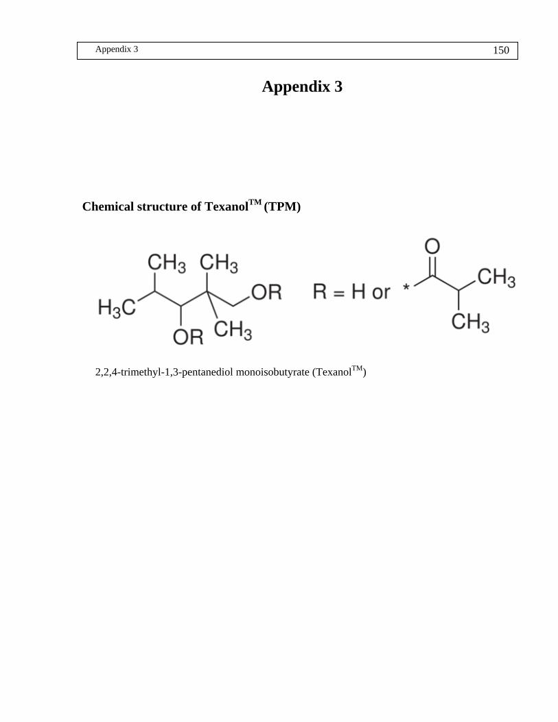
Appendix 3 150
Appendix 3
Chemical structure of TexanolTM (TPM)
2,2,4-trimethyl-1,3-pentanediol monoisobutyrate (TexanolTM)