Download - The Gravity of Experience
The Gravity of Experience
Pushan Dutt* Ana Maria Santacreu** Daniel Traca+
INSEAD INSEAD NOVA Economics and Management
March 2014
Abstract
In this paper, we establish the importance of experience in international trade for reducing trade costs and facilitating bilateral trade. Within an augmented gravity framework, we find that an additional year of experience at the country-pair level reduces trade costs by 2.0% and increases bilateral exports by 8%. The effect of experience is stronger for country-pairs that are more distant, who do not share a common border, and who lack colonial and legal ties. Further, experience raises both the extensive and the intensive margins of trade. In a dynamic trade model with heterogeneous firms and where export-experience reduces trade costs, our empirical results imply that benefits of experience are shared industry-wide and that experience lowers the variable component of trade costs. JEL Classification: F10, F14 Keywords: Gravity model; Trade costs; Experience; Extensive and intensive margin
* Corresponding author: INSEAD, 1 Ayer Rajah Avenue, Singapore 138676; Email: [email protected], Ph: + 65 6799 5498 ** INSEAD, 1 Ayer Rajah Avenue, Singapore 138676; Email: [email protected], Ph: + 65 6799 5347 + NOVA Forum Professor of Sustainable International Business, School of Economics and Management, Universidade NOVA de Lisboa, Campus de Campolide, 1099-032 LISBOA, Portugal, Email: [email protected]
1 Introduction
World trade has exploded over the last few decades, a phenomenon often associated with the decline in
trade costs. Surprisingly, according to Helpman, Melitz and Rubinstein (2008), virtually all that growth has
occurred between country-pairs that were already trading in 1970, rather than due to the emergence of trade
between new partners. Figure 1 shows that this �nding is persistent even over a longer time frame. We
use the IMF-DOTS data over the period 1948-2006 and decompose the evolution of world trade into trade
between country-pairs with strictly positive trade prior to 1950 and the emergence of trade between new
trading partners. Over the subsequent 55 years, less than 25% of the increase in world trade is attributed to
the emergence of new trading partners, and 75% to the increase in trade between partners that had strictly
positive trade prior to 1950. This despite the fact that only 31% of the possible country-pairs actually had
positive trade in 1950. The puzzle is why the decline in trade costs that contributed to the growth of trade
in established trading partners has had such a minor impact in the creation of new trade partnerships.1
At the same time, the underlying determinants of trade costs remain poorly understood (Head and Mayer,
2013a). Multiple studies have identi�ed a persistent and even rising role for gravity variables such as distance,
borders, language and colonial ties.2 Prior work, in order to reconcile these persistent e¤ects of such gravity
variables for trade, often alludes to informational costs, cultural di¤erences and the importance of business
and social networks in overcoming informal barriers to international trade (Rauch, 1999; Greif, 1994). For
instance, Grossman (1998) argues that estimated distance e¤ects are too large to be explained by shipping
costs and that cultural di¤erences and lack of familiarity account for the persistence of distance, while
Anderson and van Wincoop (2004) stress the role of information barriers, contracting costs and insecurity.
Head, Reis and Mayer (2010) attribute the decline in trade between countries that shared a colonial link
to the depreciation of trade-promoting capital embodied in institutions and networks. Head and Mayer
1We get a similar pattern even if we control for standard gravity variables such as distance and origin- and desitnation-country
size.
2 In a wide range of gravity estimates, the inhibiting in�uence of distance on bilateral trade seems to have increased since
the 1970s (Disdier and Head, 2008; Combes, Mayer, and Thisse 2006; Head and Mayer 2013), coinciding with a fall in shipping,
air cargo and communication costs and the rise of internet technologies. Borders also matter a lot - Head and Mayer (2013a)
examine 71 di¤erent estimates of the border e¤ect (based on well-speci�ed structural gravity models) and estimate that a border
is equivalent to very high tari¤s (about 43.5%) and that actual tari¤s explain a very small share of the border e¤ect. Egger
and Lassmann (2012) in their meta-analysis �nd that sharing a common language increases bilateral trade by 44%. As with
distance, they �nd not simply a persistent e¤ect but an increasing language e¤ect on trade over time. Finally, Head, Reis and
Mayer (2010) �nd that while trade declines once a colony becomes independent of the colonizer, the trade for country-pairs
that had been in a colonial relationship in the past remains 27% higher than trade of countries that were never in colonial
relationships.
1
(2013b), drawing on the analogy of dark matter, coin the term �dark trade cost�and argue that these gravity
variables capture some unmeasured and unknown sources of resistance.
Some papers attempt to directly incorporate these forces. For instance, Rauch and Trindade (2002) �nd
a substantial trade-enhancing e¤ect of Chinese networks and argue that these networks reduce information
barriers to trade.3 Anderson and Marcouiller (2002) and Berkowitz et al (2006) show that insecurity, associ-
ated both with contractual enforcement problems and opacity of regulations, lowers trade substantially. Dutt
and Traca (2010) �nd that corruption impedes trade when formal tari¤ barriers are low. Allen (2012) and
Chaney (2014) develop trade models that explicitly incorporate the search process producers use to acquire
information about market conditions and trading partners. Finally, Guiso, Sapienza and Zingales (2009)
demonstrate the importance of bilateral trust for international trade and link bilateral trust to cultural
similarities between pairs of countries.
In this paper, we take as given that there are some unmeasured trade costs, some of which are correlated
with the traditional gravity variables. Our main hypothesis is that a key factor driving the decline in such
trade costs is the cumulative experience of trade across country-pairs. When two countries start trading
with each other, a large component of trade costs is related to the novelty and uncertainty of selling in an
unfamiliar environment, identifying customer preferences, engaging with foreign shipping agents, customs
o¢ cials or consumers, and navigating an uncharted legal and regulatory context (Anderson and VanWincoop,
2004).4 Experience from repeated local interaction is e¤ective in gaining familiarity, acquiring information,
and building contacts. These in turn, contribute to dampening costs associated with the shipment, border
crossing and distribution in the destination country. Note that the e¤ects of experience may be partly
associated with the establishement of bilateral trade networks. Hence the accumulation of experience works
to overcome the informational, contractual and cultural barriers, some of which are captured by gravity
variables, suggesting that experience reduces trade costs and expands bilateral trade �ows. As a result,
countries that have a long bilateral trading relationship are likely to face lower trade costs as compared to
country-pairs that have little or no experience in trade, helping explain the dramatic growth of trade among
established country-pairs found empirically.
Our empirical speci�cation adjusts the gravity equation to account for the role of experience, which we
measure as the number of previous years of positive trade between a pair of countries. At the country-pair
3Head and Ries (1998) �nd smaller e¤ects of immigration links for Canadian bilateral trade. Bastos and Silva (2012) use
Portugese data to show that larger stocks of emigrants in a given destination, increases export participation and intensity.
4Kneller and Pisu (2011) use surveys of UK �rms and �nd that identifying contacts and building relationship with decision
makers, customers & partners are two most commonly cited export barriers.
2
level, we have su¢ cient variability in experience, both across countries and over time, that allows us to
identify the importance of experience in lowering trade costs.5 We �nd that experience has a positive and
signi�cant e¤ect on bilateral trade, a �nding that is robust to a battery of checks - di¤erent estimation
methods, accounting for endogeneity and measurement error in our experience variable, di¤erent measures
of the extensive and intensive margins, and to the use of various sub-samples or sub time-periods. For our
preferred speci�cation, our estimates imply that an additional year of experience reduces trade costs by 2%.
We also decompose the impact of experience on the extensive margin, de�ned as the number of HS-6 products
traded, and the intensive margin, de�ned as the value of exports per product. We �nd that experience has
an almost identical e¤ect on both margins of trade.
Next, we condition the role of experience on gravity variables that capture geographical, cultural, legal
and linguistic barriers, stressing their role in capturing the in�uence of informational challenges and cul-
tural di¤erences. When these barriers are high, the scope for bridging them is likely to enhance the role
of experience. On the other hand, if two countries are closer (e.g. share the same language), the e¤ect of
experience, may proceed at a faster pace, as exporters have an easier time navigating the new environment.
From this perspective, experience may facilitate trade more strongly for country-pairs where the aforemen-
tioned barriers are low. Therefore, whether experience matters more for country-pairs with higher or lower
barriers is ambiguous; an issue that we address empirically. Our results show that the e¤ect of experience
on trade �ows is stronger for country-pairs that are distant, who do not share a border, lack colonial ties
and use di¤erent legal systems. The one exception is common language, which seems to dampen the e¤ect
of experience on trade �ows, suggesting that experience does not matter in the same extent for all types
of trade barriers.6 At the same time, the interaction between experience and these gravity variables works
mainly on the extensive margin, suggesting that as country-pairs accumulate experience, trade costs become
less important for the introduction of new products, rather than for the volume of already traded products.
Our empirical results suggest that trade costs are dynamic and decline with experience. To shed light
on these �ndings, we build a dynamic version of Chaney�s (2008) model of heterogeneous �rms and �xed
costs of exports, where trade costs, both �xed and variable, decrease as experience is accumulated over time.
Further, we derive closed-form solutions for bilateral trade and extensive and intensive margins in line with
our empirical implementation. We consider two ways in which �rms can accumulate experience: �rst, we
5By contrast, �rm-level trade data is not widely available for large numbers of country-pairs and usually span short time-
series.
6This also implies that the e¤ect of gravity variables is, in fact, heterogeneous and conditional on experience. Head and
Mayer (2013b) show that the e¤ect of distance is heterogeneous with lower impact for larger trade �ows.
3
look at the case where the �rm bene�ts only from its own-experience; second, we address the case where
experience of �rms is shared across all the potential exporters. The predictions of our model for total trade
are consistent with our empirical �ndings. However, which margin of trade drives this e¤ect depends heavily
on how the �rm captures the bene�ts of experience.
When �rms bene�t only from own-experience, there is more entry in the �rst period that trade is allowed
that what the Chaney model would predict, because some less productive forward-looking �rms are willing to
make negative pro�ts in the early periods to bene�t from higher future pro�ts as they accumulate experience.
Over time, the intensive margin of trade increases, as incumbents that are accumulating experience face
lower trade costs. The extensive margin, however, does not increase over time, because non-exporters do
not bene�t from the experience of incumbents. On the other hand, when �rms bene�t from the experience
of their peers, entry in the �rst period that trade is allowed is similar to Chaney (2008), because the e¤ects
of experience are now external. Di¤erent from the previous case, the extensive margin now increases with
experience, as non-exporters see their trade costs declining from the experience of the incumbents. The
e¤ect on the intensive margin is now complex: the larger exports of incumbents (who see their variable trade
costs falling) con�ict with the entry of smaller, new exporters. Tying the model predictions to our empirical
�ndings suggests that a) experience is shared across �rms, and b) experience reduces at least the variable
costs of trade. We close with a numerical exercise where we allow for general equilibrium e¤ects.
This paper contributes to the trade costs literature in three ways. First, it highlights the role of experience
in bridging �unmeasured�trade costs associated with informational barriers and cultural di¤erences, which
provides an intuitive solution to the puzzle in Helpman, Melitz and Rubinstein (2008). Our empirical work
con�rms that these e¤ects are important and robust. Second, it develops a model where trade costs are
dynamic and evolve over time, driven by the accumulation of experience at �rm- or industry-level. Our
model introduces dynamic paths of entry into exports and of export volumes in a simple and intutive way.
Third, it leverages the predictions of the model for the extensive and intensive margin to conclude, in light
of the empirical results, that the e¤ects of experience are shared among exporters and non-exporters, which
is in line with recent literature focusing on the role of networks and search in export decisions. (Eaton et al,
2012; Chaney, 2014).
The rest of the paper is organized as follows. Section 2 augments the traditional gravity speci�cation
with experience at the bilateral level allowing for both a direct e¤ect of experience and for its e¤ect to be
moderated by traditional gravity variables; Section 3 lists the variables and data we use; Section 4 presents
our empirical �ndings; Section 5 introduces experience in a standard Chaney (2008) model to examine the
evolution of the extensive and intensive margins.
4

2 An experience-adjusted gravity equation
2.1 Trade costs and the gravity equation
Trade costs capture the extra costs that a �rm bears to sell goods in a foreign country, including (i) trans-
portation costs, enhanced by poor infrastructure and low security, (ii) border-crossing costs, associated with
tari¤s and the corruption costs and delays in institutionally weaker and highly regulated environments and
(ii) distribution costs that are heightened from dealing with distribution partners in countries where contract
enforcement is feeble and �nding the preferences of customers that are culturally and linguistically di¤erent.7
The gravity equation is the current workhorse for estimating the importance of trade costs for bilateral
trade. There are several theory frameworks supporting the gravity speci�cation, yielding the logarithm of
exports from country o (exporter/origin) to country d (importer/destination) in time t, denoted by Xod;t,
as shown below (Head and Mayer, 2013a).
lnXod;t = �o�o;t + �d�d;t � � ln �od;t + eod;t (1)
�o;t and �d;t are exporter and importer-year dummies that capture attributes of the exporting- and the
importing-country, respectively, including size and their multilateral trade resistance (Anderson and Van
Wincoop, 2003). �od;t measures bilateral trade costs, with �� as the elasticity of exports with respect to
trade costs.8 In the standard equation ln �od;t is speci�ed in terms of bilateral gravity variables, as shown
below.
ln �od;t =MXm=1
mzmod;t (2)
where zmod;t are the M gravity variables and m are parameters. Head and Mayer (2013a) perform a meta-
analysis and identify as main variables the trade and currency agreements, capturing trade policy, and
distance, contiguity, shared language, and colonial links, which measure geographic, cultural, and historical
barriers. We refer to these time-invariant gravity variables as remoteness variables.9 Substituting (2) in (1)
7Anderson and Van Wincoop (2004) estimate that trade costs are equivalent to a 170 percent ad-valorem tax equivalent for a
representative rich country, including a 21 percent for transportation costs, 44 percent for border-crossing costs and 55 percent
for distribution costs. Head and Mayer (2013) show that 72%�96% of the trade costs associated with distance and borders are
attributable to the dark sources (read unknown) sources of resistance.
8� has di¤erent interpretations depending on the micro-foundations for the gravity equation. It is the elasticity of substitution
(minus one) among varieties in Anderson and van Wincoop (2003), the parameter in the Pareto distribution of �rm productivities
in Chaney (2008) and the parameter governing the dispersion of labour requirements across goods and countries in Eaton and
Kortum (2002).
9Note that the policy variables are time-varying while the remoteness variables are time-invariant.
5

yields an estimable speci�cation.
lnXod;t = �o�o;t + �d�d;t �MXm=1
� mzmod;t + eod;t (3)
2.2 Experience and trade costs
Exporting to a new geographic market entails the discovery of (i) the cheapest, most reliable transport;
(ii) the best way to get goods through customs, (iii) the right partner for distributing and promoting the
goods locally or (iv) the preferences and dispositions of customers. Eaton et al. (2012) and Freund and
Pierola (2010) emphasize learning in a destination country, where producers need to incur costs to �nd new
buyers or new products.10 Allen (2012) models a search process to acquire market information, and, for
regional agricultural trade in the Philippines, �nds that 93% of the observed gravity relationship is related
to informational frictions rather than transport costs.
Although �rms may engage in pre-entry research, experience is a vital element of the process. The initial
contact with a new market environment unavoidably raises unexpected challenges that push the �rm to �nd
quick, imperfect solutions that imply higher trade costs. Experience with the local reality helps the �rm
gain familiarity and �nd better, cheaper solutions for future shipments, lowering trade costs. For instance,
Artopoulos, Friel and Hallak (2010) use four detailed case studies of export �rms in Argentina to show
that export success stems from a �rm�s experience in the business community of the destination country.
Similarly, Kneller and Pisu (2011) show that the best predictor of whether a particular �rm identi�es an
export barrier as relevant is explained almost exclusively by experience measured as the number of years the
�rm has been exporting. Our hypothesis is that trade costs fall when experience by exporters increases.
In addition to bene�ting the �rm, experience is also likely to be shared among networks of �rms, who
may be organized into industry associations, by worker mobility across �rms, and/or by the use of common
consultants prior to entering an export market. Clerides et al. (1998) examine the role of geographic and
sectoral spillovers on the export decision for the Colombian plants and �nd some evidence for such spillovers.
Aitken et al. (1997) examine the role of spillovers on exporting by plants in Mexico. They �nd that the
presence of multinational exporters in the same industry and state increases the probability of exporting by
Mexican �rms. This implies that experience acquired historically by some exporters contributes to increased
familiarity by fellow exporters, and even crosses over to non-exporters.11
10 In contrast, in Albornoz et al (2012) uncertainty is not destination-speci�c and �rms learn about export pro�tability as a
whole.
11Eaton et al (2012) use Colombian data to show that �rms that were initially non-exporters within a decade account for
nearly a quarter of total exports. Firms in their model learn from both own experience and the experience of rivals.
6
To the extent that the bene�ts of experience are related to the familiarity with local context it creates,
the cumulative interaction between exporters and the destination country environment is a natural measure
of (stock of) experience. Letting Eod;t denote the stock of experience in trading with destination-country d,
we capture the hypothesis that experience lowers trade costs, by de�ning the following experience-adjusted
speci�cation for trade costs
ln �od;t =MXm=1
mzmod;t � �odEod;t where �od > 0 (4)
Assuming, for now, that �od = �, 8od (constant for all origin�destination pairs), we can use this in (1) to
obtain an estimable speci�cation for the gravity equation that accounts for the e¤ect of experience.
Simpli�ed Experience-Adjusted Gravity Equation
lnXod;t = �o�o;t + �d�d;t �MXm=1
� mzmod;t + ��Eod;t + eod;t (5)
2.3 Remoteness and the impact of experience
Experience is also likely related to the informational barriers and cultural di¤erences that it helps bridge. To
the extent that these barriers are heterogenous, the impact of experience is also likely to vary across country
pairs, challenging the notion that �od in (4) is constant. As mentioned earlier, several authors have argued
that these informational and cultural barriers, while di¢ cult to measure, are strongly associated with the
subset of gravity variables that measure remoteness, at the level of the country-pair. Given the di¢ culty in
comprehensively measuring all cultural and information barriers that de�ne the scope for experience, and
to the extent that the remoteness also re�ects such trade barriers, we argue that the variation in �od across
country-pairs is associated with the subset of gravity variables measuring remoteness. Following Head and
Mayer (2013a), we stress proximity, contiguity, shared language, shared legal systems and colonial links as
the remoteness variables of interest, and express �od in terms of the these variables, as shown below
�od = �+P
m2� �m zmod > 0 (6)
where � denotes the subset of gravity variables that capture remoteness. After substituting in (4) and then
in (1), this yields:
7

Generalized Experience-Adjusted Gravity Equation
lnXod;t = �� Eod;t �Xm2�
� m zmod +Xm2�
��m zmodEod;t (7)
�X
m2Mn�
� mzmod;t + �o�o;t + �d�d;t + eod;t
Interestingly, the role of remoteness on the e¤ect of experience, depicted by the �m´s, is non-trivial. To
see this, let us take language as an example and see how it a¤ects the impact of experience on trade costs.
On one hand, in the long-term, experience is likely to have a stronger e¤ect for exporters from countries that
do not share the same language. They start with higher trade costs associated with the language di¤erence,
which are eventually brought down as the exporter learns the new language or �nds a local contact that
speaks its language, for example. From this perspective, experience should matter more when the two
countries face higher barriers in the sense that they do not share a language. On the other hand, in the
short-term, if the two countries share the same language, the process of acquiring familiarity proceeds much
faster, through conversations with locals or by reading local literature, for example. From this perspective,
experience should matter more, when the two countries face lower barriers by sharing a common language.
Generalizing to the other time-invariant gravity variables that capture remoteness, this implies an ambiguous
sign for the �m´s in (7): for a variable m in �, if �m > 0 then experience matters more for more remote
countries in facilitating trade, and if �m < 0 then experience matters more for less remote countries.
Note that, under (7), the traditional e¤ect of gravity variables capturing remoteness is conditional on
experience, i.e. for m in �, d lnXod;t=dzmod = �(� m + �mEod;t). The fact that the impact of experience
on trade �ows (�m) may increase or decrease with remoteness, implies symetrically that the e¤ect of the
traditional gravity variables on trade also varies with experience. When �m > 0, experience lowers the e¤ect
of remoteness on trade �ows. When �m < 0, experience actually increases the impact of remoteness beyond
its initial level. This means that the e¤ect of each remoteness variable is also heterogeneous and conditional
on experience. Estimating the gravity equation without accounting for experience implies capturing the
e¤ects of the gravity variables for the average level of experience for the country-pairs in the sample.
3 Data and Variables
3.1 Experience
The bene�ts of experience depend on the accumulation and intensity of interactions between exporters and
the destination country environment - e.g. the number of shipments or the number of years of exports
8

(Kneller and Pisu, 2011). An important empirical challenge is the need for precision and variability in the
variables that measure experience. Available �rm-level datasets cover relatively few exporting countries and
cover short time-spans yielding limited dispersion and potential measurement error in experience measures.
Therefore, we choose to measure experience at the country-pair level, which is also in line with standard
gravity models. In this context, experience must be seen as an aggregation of the experience of all the
exporter and importer �rms involved in trade from o to d, including bene�ts that spill over across �rms.
We proxy experience using the number of years for which the country-pair has had strictly positive
trade. We prefer this to the alternative of taking the accumulated value of exports because the latter is
in�uenced by the unit value of exports. In this case, experience would be in�uenced by changes in the
sectoral composition of country´s exports, both in terms of comparisons across countries and its evolution
in time, creating unwanted spurious variation.12
We use the International Monetary Fund�s Direction of Trade Statistics (DOTS) to construct our expe-
rience variable. This database provides data on bilateral exports from 208 exporters to 208 importers over
the time period 1948-2006. For any pair of countries o and d at time t in our sample, we calculate experience
as the number of years where o had strictly positive exports to d up until the year t � 1. Figure 2 shows
the distribution of the length of trading relationship in 2006, for all country-pairs (including those with
zero trade �ows in that year): 4.2% of the country-pairs have traded for 0 years, the median and the mean
trading relationship lasted for 14 and 21.7 years, respectively. The experience variable is right-censored for
country-pairs that had strictly positive trade in 1948: 6.8% of the country-pairs have a trading relationship
at the maximum of 58 years (2006-1948). Finally, the peak around 13 years arises from the breakup of the
Soviet Union and of Yugoslavia and Czechoslovakia in 1992.13 In robustness checks, we will account for zero
trade, for the censoring of the experience variable and for the formation of new countries in Eastern Europe
around 1992-1993.
To address the potential for measurement error, we also use an alternative dataset from the Correlates
of War (COW) Project, which tracks bilateral trade from 1870-2006 (supplementing the DOTS data with
data from Barbieri (2002) and Barbieri, Keshk and Pollins (2012). In 2006, the median trading relationship
was 23.2 years. The correlation between the COW and the DOTS measures exceeds 0.8 for each of the
12Measuring experience at the product-country-pair level is di¢ cult since much of the disaggregate data are of recent vintage.
13 In constructing the experience variable, we coded all countries that were formerly part of the Soviet Union, Czechoslovakia
and Yugoslavia as new countries and set experience to zero in their �rst year of trade after 1992. The exceptions are trade with
the Soviet Union which was merged with Russia and with West Germany which was merged with Germany. These choices,
while reasonable since exporters plausibly faced a new environment, may also create measurement error in experience.
9

years in our sample (1988-2006), rising to 0.91 in the year 2006.14 The COW data, by going further back
in time, requires fairly strong assumptions about shifts in country identities through division, uni�cation,
and emergence from colonial rule. For instance, the COW-based experience assumes trade with the Austro-
Hungarian as trade with both Austria and Hungary and assigns trade with Zanzibar as trade with Tanzania.
More importantly, COW provides trade data on former colonies in Asia, Africa and Latin America only when
they become independent. In contrast, the DOTS data captures bilateral data for these countries prior to
colonization. Finally, much of the data is missing prior to 1948. Therefore, experience constructed on the
basis of this data is also not free of measurement error. For this reason, we use the DOTS-based measure
as our main measure of experience, and use the COW-based measure to examine the impact of censoring at
58 years.
3.2 Bilateral trade and extensive and intensive margins
We follow the literature and provide a decomposition of the empirical e¤ects of experience on the extensive
and the intensive margins. Our decomposition emerges from a simpli�ed model with �rm-heterogeneity,
where bilateral exports Xod;t can be decomposed as
Xod;t = Nod;t � xod;t (8)
the product of the extensive (Nod;t), i.e. number of sectors/goods traded,and the intensive margins (xod;t),
i.e. the volume of trade per product/sector. Since the gravity speci�cation is implemented in terms of the
natural logs, the sum of the estimated coe¢ cients for the two margins equals the coe¢ cient on the standard
gravity speci�cation with total bilateral exports. Following Eaton, Kortum and Kramarz (2004), Bernard et
al. (2007), and Flam and Nordstrom (2006), the bilateral extensive margin is a count of the number of HS-6
products exported from country o to country d at time t, while the bilateral intensive margin is de�ned as
the exports per product.
The lack of disaggregated data in DOTS (used to measure experience) prevents us from constructing
the intensive and extensive margins, which we need as dependent variables, with this data. Hence we use
UNCTAD�s COMTRADE database to obtain bilateral trade �ows, and the extensive and intensive margins
of trade. COMTRADE provides data on bilateral trade between pairs of countries at the Harmonized System
6-digit (HS-6) level of disaggregation.15 We construct a database on the trade �ows and their extensive and
14We restrict our sample to 1988-2006 since we decompose total trade into an extensive and intensive margin based on
COMTRADE HS-6 data. The latter are available only from 1988 onwards.
15UNCTAD provides the HS-6 data over the period 1988-2006 for 183 importers and 248 exporters. There are 5017 product
10

intensive margins, for the period 1988-2006. For each year in our sample, our data spans more than 99% of
all world trade.
3.3 Gravity variables
Our list of trade cost determinants come from the meta-analyses of Disdier and Head (2008) and Head and
Mayer (2013a). The remoteness gravity variables include geographic distance, contiguity, common language
and colonial links. Geographic distance is measured as the logarithm of the distance (in kilometers) between
the two most populous cities. Contiguity is a dummy variable that takes the value 1 if the country-pair
shares a common border. Common language is captured by a dummy that equals 1 if the country-pair
shares a common o¢ cial language. Colonial links is measured using two variables, that take the value 1 if
a country-pair was ever in a colonial relationship (one country was the colonizer and the other colonized or
vice versa). Data on these variables are obtained from the CEPII gravity databases (www.cepii.fr). We also
create a dummy variable that captures common legal origins, from Glaeser and Shleifer (2002) (other �ner
classi�cations of civil law, Scandinavian law did not seem to matter).
As suggested in our speci�cation, we include also policy-related gravity variables, from Head and Mayer
(2013b), which we consider impervious to experience. We include one variable related to currency sharing
and three related to preferential market access: multilateral, bilateral, and unilateral. We use a dummy
variable that captures membership in a currency union. Data on currency unions are from Head, Ries and
Mayer (2010). Multilateral market access is captured by two dummy variables: one takes the value 1 if both
trading partners are members of the GATT/WTO and 0 otherwise; the other takes the value 1 if neither
countries in a country-pair are WTO members. The category where only one country in a pair is a WTO
member is the omitted category. Bilateral preferential trade arrangements are captured by a dummy variable
which takes the value 1 if both trading partners are members in a preferential trade arrangement (PTA).
Data on WTO membership and PTAs are from the CEPII gravity databases (www.cepii.fr) and updated
via the WTO website (www.wto.org). Unilateral preferential access is in terms of the Generalized System
of Preferences (GSP) where trade preferences are granted on a non-reciprocal basis by developed countries
to developing countries. We code a dummy variable as 1 if the importing county grants a GSP to exporter.
GSP data are from Andrew Rose�s website and updated from the WTO website.
categories or lines at the HS-6 level.
11

4 Empirical Findings
4.1 Simpli�ed experience-adjusted gravity
We start by examining the role of experience by estimating the simpli�ed experience-adjusted gravity in (5),
using the measure of experience outlined above. The estimation of the gravity equation has been subject
to an intense econometric debate over the last decade. In line with Head and Mayer (2013a), our baseline
results rely on least-squares estimation of the panel, using country-speci�c �xed-e¤ects and with standard
errors adjusted for clustering on country-pairs. We address also the potential for biases through a series of
robustness checks. First, we look at the potential for biases associated with our data on experience, namely
the censoring and endogeneity of the experience variable. Second, we look at biases that are pervasive
in the gravity literature, such as the presence of structural zeros and heteroskedastic errors (Santos Silva
and Tenreyro, 2006) or the omitted changes in the distribution of exporting �rms (Helpman, Melitz and
Rubinstein, 2008).
4.1.1 Baseline results
Table 1 presents our baseline estimates for (5). Columns (1)-(3) examine the impact of experience (based
on the DOTS data) on bilateral trade, extensive and intensive margins respectively. We con�rm the role
of experience on all three variables of interest - a one standard deviation increase in experience results in a
50% increase in the extensive and intensive margins and a 100% increase bilateral trade. From equation (5)
and Table 1 the coe¢ cient on experience equals �� = 0:06. If � is the Pareto shape parameter from Chaney
(2008) or the parameter governing the dispersion of labour requirements across goods and countries in Eaton
and Kortum (2002), then a reasonable value is � = �4. Our estimate in Table 1 implies that trade costs
decline by 1.5% for every year of experience.16
Con�rming the results established in the literature, the direct e¤ect of virtually all gravity variables
identify them as trade costs. Proximity, contiguity, colonial relationships, sharing of languages and similarity
of legal systems foster trade, through both the intensive and the extensive margins; with the exception of
contiguity and common language which have an insigni�cant e¤ect on the intensive margin. The estimates
of the policy variables are also in line with the literature: WTO and PTA increases trade, with e¤ect of the
WTO mainly on the extensive margin (see Dutt, Mihov and Van Zandt, 2013), while the common currency
dummy increases total export via the intensive margin.
16 If we estimate � in a cross-section for each year, instead of in a panel, it takes values ranging from 0.052 to 0.097. Moreover,
the coe¢ cient estimate is signi�cant in each year.
12

It should be noted that, if we estimate a traditional gravity equation without experience as an independent
variable we obtain coe¢ cients on the gravity variables that are signi�cantly higher in absolute terms (16%
for distance and legal system; 3% for contiguity; 6% for colonial link; and 39% for language). In other words,
accounting for experience signi�cantly reduces the magnitude of the coe¢ cients for the traditional gravity
variables.
4.1.2 Censoring and Omitted Variables
Our experience variable based on the DOTS data is right-censored at 58 years. To account for the right-
censoring, we added a dummy variable for all DOTS-based censored observations (with experience at 58).
Including this does not change either the sign, signi�cance or magnitude of the estimates.17 Next, we
sequentially dropped 14 countries that were part of the Soviet Union, the 4 countries that formerly constituted
Yugoslavia, and �nally Czech Republic and Slovakia. In all cases, we observe a marginal rise in the coe¢ cient
of experience for both overall trade and the extensive margin, but no change for the intensive margin.
As an additional check, we estimate the gravity equation using the COW dataset as a measure of expe-
rience, which has data going back to 1870. Columns (4)-(6) provide estimates, con�rming that experience
signi�cantly increases both overall trade and each of the two margins. The coe¢ cient on experience halves as
compared to the coe¢ cient when we use the DOTS-based measure of experience. Examining the distribution
of the two experience variables, we �nd that for nearly 90% of the observations, the two measures are close
to one another. Conditional on the COW experience variable exceeding the DOTS experience variable, 80%
of the COW based experience variable take a value close to twice that of DOTS based experience variable.
Given that these are observations that correspond to large trade �ows, the decline in the coe¢ cient on
experience for the COW measure is not surprising.
Another concern is that omitted variables may drive both the experience measure and trade �ows. In
particular, omission of some determinant of �od;t which may have played a role in the decision to initiate
exports from o to d, may create endogeneity bias, as experience may simply be capturing the e¤ect of this
determinant on the dependent variables. To account for this, we experimented multiple bilateral gravity
variables as additional controls. These include the share of migrants from destination in the origin country
(to capture networks,) a common religion dummy from Helpman, Melitz and Rubinstein (2008), a dummy
17Dropping the censored observations (Austin and Brunner, 2003) entails removing all country-pairs that had strictly positive
trade in 1948. Since the increase in the volume of trade since then is mainly attributed to the expansion of trade between these
pairs, rather than the emergence of new trading partnerships (Helpman, Melitz and Rubinstein, 2008), we lose 62.5% of our
observations, that accounts for a majority of world trade.
13

that takes the value 1 if both countries are democracies (positive Polity score), political ideology of the ruler
in power (coding ideology as left-wing vs. right wing from the Database of Political Institutions), a dummy
for country-pairs that were part of the same country in the past (e.g., India and Pakistan,) and further
re�nements of the colonial links and language dummies (see Dutt and Traca 2010). Our results remain
una¤ected by these permutations.
A second methodology to address the potential omitted variables bias is to add country-pair dummies
to the standard speci�cation of the trade cost �od;t. These dummies will account for all time-invariant
bilateral trade costs, including those that may be responsible for the initiation of trade and the extent of
experience. Note that, to prevent collinearity, we must remove all time-invariant bilateral variables; namely,
those capturing dimensions of remoteness. Columns (7)-(9) present the estimates. Here we �nd a stronger
role for experience - the coe¢ cient continues to be signi�cant and there is a 40% increase in the magnitude
of the e¤ects.18 Again, if we assume � = 4, our estimates imply that an additional year of experience for
a particular country-pair reduces their trade costs by 2%. Overall the results suggest that even accounting
for time-invariant variables that may have a¤ected the decision at the time that trade started and that may
continue to impact trade today, we �nd a strong role for experience.
4.1.3 Accounting for Zeros and Heteroskedasticity
Recent papers by Helpman, Melitz and Rubinstein (2008), Anderson and van Wincoop (2004), Evenett and
Venables (2002), and Haveman and Hummels (2004) all highlight the prevalence of zero bilateral trade �ows.
For the bilateral trade data over the period 1988-2006, 37% of all possible bilateral trade �ows show a zero
value. Unobserved trade costs can endogenously create zeros and taking logs removes them from the sample,
creating selection bias. In accounting for zeros, the �rst question to consider is whether they are statistical,
in the sense that they occur due to rounding or the existence of thresholds, or structural, in the sense that
unobserved trade costs of exporting may lead to zeros in the trade matrix. We address each of these in turn.
Statistical zeros can arise either when trade is reported only if it exceeds a threshold or when importers
report trade aggregated across countries. We follow the procedure of Eaton and Kortum (2001) who use a
Tobit speci�cation to account for statistical zeros.19 The e¤ect of experience, accounting for the presence
18These within-estimates imply that a one standard deviation increase in experience results in a 71% increase in the extensive
margin, a 74% increase in the intensive margin and a 145% increase in bilateral trade.
19The methodology assumes that we observe trade only if trade exceeds some threshold level a: Below this minimum level a;
zero trade is recorded. To implement this, we calculate destination-year speci�c censoring points: adt = minofXod;tg as the
minimum value of trade across all exporters to each destination each year. We then replace the observed zeros in the trade
matrix by adt and estimate this in a Tobit speci�cation with destination-year speci�c censoring points.
14

of zeros, is shown in Columns (1)-(3) of Table 2. We con�rm that experience signi�cantly in�uences both
margins of trade, with a signi�cant increase in the coe¢ cient for the intensive margin, as expected; while
the coe¢ cient remains the same for the extensive margin (because for 99.9% of the cases the censoring point
is set to 1 (0 in log terms)).
Second, Helpman, Melitz and Rubinstein (2008), henceforth HMR (2008), argue that the zeros in the
trade matrix are not statistical but structural, due to �xed costs of exporting. They show that, in this
case, �rms self-select (or not) into exporting, which causes not just a selection bias but also a heterogeneity
bias, due to changes in the composition of �rms that export. We adopt the HMR (2008) methodology to
account for these biases. In the �rst-stage, we estimate a probit that predicts the probability of having
positive trade, for each year in the panel, %od;t, using the gravity variables and country-�xed e¤ects.20 For
the exclusion restrictions, we follow HMR (2008) and use a common religion index:P
k(Rk;o�Rk;d);where
Rk;j is the share of religion k in country j (j = o; d).21 HMR (2008) show that including a polynomial in
�z�od;t = ��1�%od;t
�+ ���od;t (where � is the cdf of the unit-normal distribution and ��
�od is the inverse Mills
ratio) controls for �rm-level heterogeneity and self-selection.
The results for the second-stage regression (which also uses country-year �xed-e¤ects), including the
bias-correcting variables, are shown in Columns (4)-(6) of Table 2.22 We con�rm that experience increases
bilateral trade, on the extensive margin and the intensive margin of exports, with coe¢ cients very similar
to those in the baseline speci�cation of Table 1. The inverse Mills ratio and the polynomial in �z�od;t are
signi�cant at 1%, with signs similar to ones obtained in HMR (2008), showing the importance of correcting
for the biases associated with structural zeros.
Finally, we use the methodology of Santos Silva and Tenreyro (2006) who show that log-linear speci�-
cation of the gravity model in the presence of heteroskedasticity leads to inconsistent estimates.23 Their
methodology treats bilateral trade as a count variable and uses the Poisson Pseudo-Maximum Likelihood
(PPML) to estimate the coe¢ cients. Since the dependent variable is trade, rather than the log of trade, it
20We use the IMF�s DOTS database to code zero vs. positive exports between country-pairs, and con�rm these by cross-
checking with the COMTRADE and the World Trade Flows Database.
21The set of religions we use is more comprehensive than that of HMR (2008), including k = Bahais, Buddhist, Chinese Uni-
versist, Christianity, Confucian, Ethnoreligionist, Hinduism, Jainism, Judaism, Islam, Shinto, Sikhism, Taoists and Zoroastrian.
The data are from the Association of Religion Data Archives.
22Since some countries export to, or import from, all other countries in a particular year, �xed exporter and importer e¤ects
cannot be estimated in the probit equation, and all observations with that particular exporter or importer are dropped. As a
result, the number of observations declines to 220,366.
23 If the error term in the standard log speci�cation is heteroskedastic, its log is not orthogonal to the log of the regressors,
leading to inconsistent estimates of the gravity elasticities.
15
also accounts for zeros in the trade matrix. Since our panel data yields 5513 country-year dummies, we apply
the PPML methodology for a single year with exporter and importer �xed-e¤ects, to obtain convergence.24
The estimates for year 2004 are shown in Columns (7)-(9) of Table 2. Here the coe¢ cient on experience
for the extensive and intensive margins remains strongly signi�cant and virtually unchanged compared to
the HMR (2008) speci�cation. The coe¢ cient on experience for overall trade declines somewhat but remains
signi�cant.
4.2 Generalized experience-adjusted gravity
In this section, we allow for heterogeneity in the e¤ects of experience, examining whether the coe¢ cient on
experience, �od, varies across country-pairs according to their geographical, cultural and linguistic remote-
ness. As discussed before, in the linear speci�cation, the expected sign of the mediating e¤ects of remoteness,
�m, is ambiguous. Greater remoteness increases how much the pair can bene�t from experience, while lower
remoteness increases the speed at which the bene�ts from experience accrue.
We estimate equation (7), interacting our DOTS-based experience measure with each of the time-invariant
remoteness variables.25 The results for total exports and for the extensive and intensive margins are shown
in Table 3A. The results for the extensive margin, in Column (2), mirror the �ndings for total exports in
Column (1) while for the intensive margins, the results in Column (3) are varied.
To evaluate the moderating e¤ect of each remoteness variable of experience on total trade and the
two margins, we report in Table 3B, the (average) marginal e¤ects of experience for various values of the
remoteness variables. These are based on the coe¢ cient estimates in Table 3A. Note that the remoteness
variables, with the exception of distance, are dummies. Therefore for distance we report the marginal e¤ects
at one standard deviation above and one standard deviation below the mean. The average marginal e¤ect
of experience for total exports, evaluated at the sample mean of each remoteness variable, is 0.06: 0.029
for the extensive margin and 0.031 for the intensive margin. These are nearly identical to the estimate
obtained in Column (1) of Table 1. At the same time, experience positively a¤ects bilateral trade and the
two margins regardless of the exact value of the remoteness variable. However, the e¤ect of experience on
exports is stronger in countries that are further away, non-contiguous, have no colonial links and do not share
a common legal system. In contrast, the role of experience for exports is stronger when countries share a
24A well-known problem with the PPML estimator is that the maximum likelihood function does not converge when there
are many dummies.
25 In the empirical implementation, while distance is a direct measure of remoteness, contiguity, linguistic, colonial and legal
ties are inverse measures of remoteness.
16

common language. That is, experience matters more when a country-pair shares a common language, while
for all other remoteness variables, experience matters more when the country-pairs are more remote.
The second column shows that the e¤ect of experience on the extensive margin is moderated in exactly
the same way as that for bilateral exports. The impact of experience is stronger for those that are distant,
non-contiguous and lack colonial and legal links. However, sharing a common language strengthens the
e¤ect of experience. For the intensive margin in the third column, we �nd that the e¤ect of experience does
not depend on any of the remoteness variables, except distance and colonial ties. For countries that are
proximate and have colonial links, experience matters less for the intensive margin.
The speci�cation in Table 3A also implies that the estimates for the standard gravity variables are
conditional on experience. In Table 3C, we compute the e¤ect of each variable on bilateral exports, at
varying points of the sample distribution of experience. For comparison, the �rst two columns report the
median and mean coe¢ cient estimates from the meta-analysis of Head and Mayer (2013a).26 Geographical
proximity, a common border and legal systems and colonial links are important facilitators of trade, but
their impact diminishes with experience. In other words, while our estimates con�rm their importance for
trade �ows, the accumulation of experience by country-pairs diminishes their importance over time. This
said, our results con�rm the nature of these variables as trade costs, even for large values of experience. For
example, distance always impedes trade while sharing a border always facilitates trade, regardless of how
long the countries have been trading; only when countries have been trading close to 182 (63) years, does the
distance (contiguity) e¤ect fade to zero. The exception is common language - sharing a language enhances
trade and its e¤ect increases with experience which is in line with Egger and Lassman (2012) who �nd an
increasing e¤ect of language over time.
Overall, these results suggest that the coe¢ cient of standard gravity variables are conditional on experi-
ence, and thereby heterogeneous across country-pairs and over time. To some extent, this can account for
varying estimates of coe¢ cients of these gravity variables. Not accounting for experience means that the
coe¢ cients capture the e¤ect of these variables at some mean level of experience which depends critically on
the sample time period and the sample used to estimate these coe¢ cients.27
26Head and Mayer (2013a) in their meta-analysis of 159 papers and 2500 gravity estimates report the median and mean
estimates of commonly used gravity variables. They do not report average estimates for common law.
27Comparing our distance estimates to the meta-analysis of Head and Mayer (2013a) we see that the coe¢ cient of distance
coincides only when experience is close to 39 years. This suggests that the gravity speci�cations in their meta-analysis include
country-pairs that have been trading for around that time, on average.
17
4.2.1 Robustness Checks
We are able to replicate our results nearly exactly when we use the measure of experience based on the COW
data or when add a dummy variable for countries whose experience is censored at 58.28 These estimates
are not presented for reasons of space. We do not estimate a speci�cation with country-pair �xed-e¤ects
since these absorb all time-invariant gravity variables, rendering the interpretation of the interaction terms
di¢ cult.
Table 4 examines the robustness of our results to the presence of zeros, heterogeneity and selection bias
by using the same Tobit and HMR (2008) speci�cation as before. Overall, the impact of experience on
trade costs is nearly identical to the previous model, for total exports and the extensive margin. In the
Tobit speci�cation, the di¤erences are that sharing a common law system increases the intensive margin,
but experience moderates this e¤ect, and that sharing a common language increases the intensive margin,
an e¤ect that becomes stronger with experience. With the HMR (2008) correction, the results remain
virtually unchanged except that the impact of virtually all trade cost determinants is smaller in absolute
terms, capturing the correction of the bias associated with heterogeneity. As before, the inverse Mills ratio is
signi�cant and the polynomial terms in �z�od;t are signi�cant in all regressions, with signs similar to the ones
obtained in HMR (2008), con�rming the importance of correcting for heterogeneity bias.29 30
Next we used alternate weighted measures of the extensive and intensive margins, following Feenstra
and Kee (2008). We obtain nearly identical results with these alternate measures of the margins. We also
estimated coe¢ cients for various country sub-samples, by classifying countries as OECD vs. non-OECD. The
strongest role for experience (both direct and interacted with the gravity variables) are for the sub-sample
when both countries in a country-pair are outside the OECD, followed by when exactly one country in a
pair is in the OECD. The weakest role for experience is when both countries are OECD members.
Summing up our empirical results, we �nd fairly strong evidence for the role of experience in a¤ecting
bilateral trade, through the extensive and intensive margins of exports. The e¤ect on the extensive margin
suggests that experience in exporting a subset of HS-6 lines increases the probability of exporting other
HS-6 lines. At the same time, the coe¢ cient on the intensive margin suggests that experience matters at
28 In the latter speci�cation, we also interacted this dummy with the gravity variables.
29Since it can be argued that the common religion dummy is not a plausible exclusion restriction, especially for the extensive
margin (which is a¤ected by both �xed and variable trade costs) we tried one additional permutation. We dropped the exclusion
restriction and relied for identi�cation on the non-linearity of the inverse Mills ratio. We get nearly identical results to those
reported in Table 4.
30Convergence becomes an issue with the PPML methodology when we use multiple interaction terms. However, with one
interaction at a time, we obtain very similar results.
18
the level of increasing exports in each product line. These �ndings are robust to censoring problems and
to demanding speci�cations to account for omitted variables, which may a¤ect our experience variable. We
account also for traditional concerns in the estimation of the gravity equation such as bias due to zeros,
heteroskedasticity in a log-linear speci�cation, and changes in the composition of exporting �rms. When
looking at the role of remoteness variables as determinants of the impact of experience (captured by their
interaction), we �nd that a stronger role for experience in more remote countries. Common language is
the only exception. Symmetrically, this means that experience works to bridge these remoteness variables,
reducing their trade-inhibiting e¤ect over time.
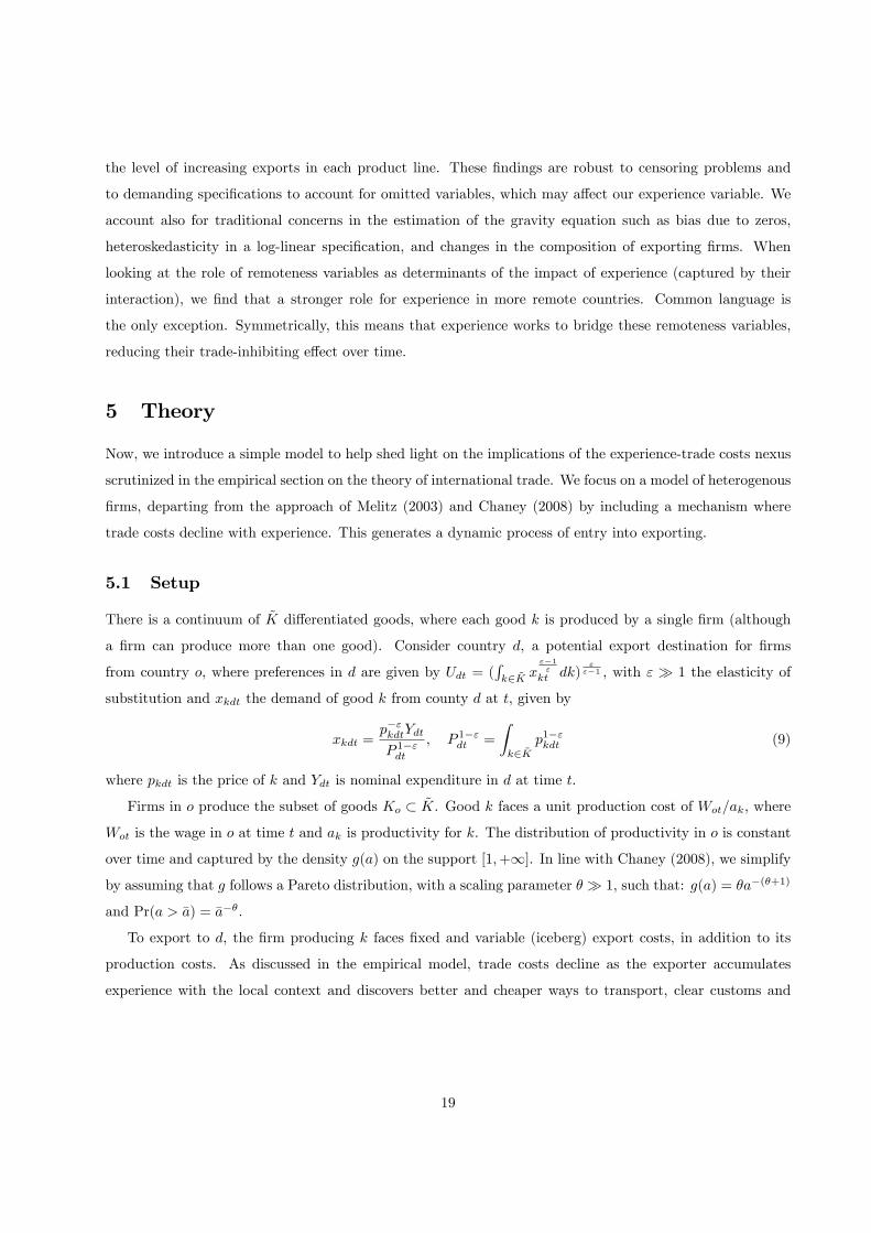
5 Theory
Now, we introduce a simple model to help shed light on the implications of the experience-trade costs nexus
scrutinized in the empirical section on the theory of international trade. We focus on a model of heterogenous
�rms, departing from the approach of Melitz (2003) and Chaney (2008) by including a mechanism where
trade costs decline with experience. This generates a dynamic process of entry into exporting.
5.1 Setup
There is a continuum of ~K di¤erentiated goods, where each good k is produced by a single �rm (although
a �rm can produce more than one good). Consider country d, a potential export destination for �rms
from country o, where preferences in d are given by Udt = (Rk2 ~K x
"�1"
kt dk)"
"�1 , with " � 1 the elasticity of
substitution and xkdt the demand of good k from county d at t, given by
xkdt =p�"kdtYdt
P 1�"dt
; P 1�"dt =
Zk2 ~K
p1�"kdt (9)
where pkdt is the price of k and Ydt is nominal expenditure in d at time t.
Firms in o produce the subset of goods Ko � ~K. Good k faces a unit production cost of Wot=ak, where
Wot is the wage in o at time t and ak is productivity for k. The distribution of productivity in o is constant
over time and captured by the density g(a) on the support [1;+1]. In line with Chaney (2008), we simplify
by assuming that g follows a Pareto distribution, with a scaling parameter � � 1, such that: g(a) = �a�(�+1)
and Pr(a > �a) = �a��.
To export to d, the �rm producing k faces �xed and variable (iceberg) export costs, in addition to its
production costs. As discussed in the empirical model, trade costs decline as the exporter accumulates
experience with the local context and discovers better and cheaper ways to transport, clear customs and
19

distribute in country j. We model this by setting the variable and �xed trade costs of k to j at t as a function
of experience, denoted by Ekdt � 0, as follows:
�kdt =
8<: ~�de$0Z���Ekdt for Ekdt � E
~�de$0Z���E for Ekodt > E
; Fkdt =
8<: ~Fde�0Z��FEkdt for Ekdt � E
~Fde�0Z��FE for Ekdt > E
; (10)
�kdt and Fkdt are the iceberg and �xed costs, respectively, to export k to d at t. Z is a vector of gravity
variables (including remoteness and policy variables), with $ � 0 and � � 0 capturing their impact on
iceberg and �xed trade costs, respectively. ~� and ~F are residuals that capture non-identi�able determinants
of trade costs and can be country-pair speci�c. We allow trade costs to decline with experience, taking �� > 0
and �F > 0 as scalars that capture the impact on iceberg and �xed costs, respectively. E is the upper bound
on experience, which yields a lower bound for trade costs given by ~�de$0Z���E � 1 and ~Fde�0Z��FE � 0.
This model reverts to Chaney (2008), when �� = �F = 0, where e$0Z~� and e�0Z ~F become trade costs.
5.2 Entry into exports
The inclusion of time requires a historical dimension for the exports from o to d. In the beginning of time
~�d and ~Fd are prohibitive ( ~Fd = ~�d = +1), such that no �rm from o ever considers exporting to d. There
is a probabilistic event that lowers ~� and ~F to a level where exports may begin. We will denote by t = 0 the
time of this event.
After that, �rms in o must decide whether and how much to export to d. Firms are forward-looking.
Assume, for now, that once a �rm starts to export, it remains an exporter forever.31 Then, the key decisions
are when to begin exporting and how much to export. The discounted value of export pro�ts at time 0 for
a �rm that begins exporting k to d at tk � 0 is given by
V (tkjak) = 0 +
Z +1
tk
e��tRktdt (11)
where Rkt =
�pkt �
�ktWt
ak
�xkt � Fkt
where we have omitted the o subscript in W and the od subscripts in x, p, � , and F (and later in P and Y ).
Rkt refers to the �rm�s pro�ts.
In accordance with our empirical approach, we capture experience using the number of years of positive
trade. Then, as the bene�ts of experience do not depend on the volume of exports, the pricing decision is
static, and the traditional CES mark-up rule, pkt = ("="� 1) �ktWt=ak, yields the value of exports to d as
xkt =
�"� 1"
ak�ktWt
�"�1Yt
P 1�"t
(12)
31This is true in equilibrium, since there are no factors that could make the �rm leave afterwards.
20
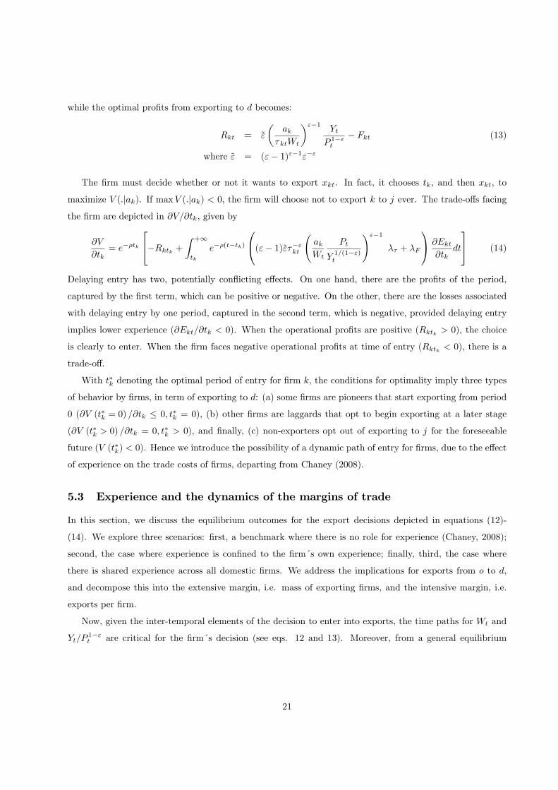
while the optimal pro�ts from exporting to d becomes:
Rkt = ~"
�ak
�ktWt
�"�1Yt
P 1�"t
� Fkt (13)
where ~" = ("� 1)"�1"�"
The �rm must decide whether or not it wants to export xkt. In fact, it chooses tk, and then xkt, to
maximize V (:jak). If maxV (:jak) < 0, the �rm will choose not to export k to j ever. The trade-o¤s facing
the �rm are depicted in @V=@tk, given by
@V
@tk= e��tk
24�Rktk + Z +1
tk
e��(t�tk)
0@("� 1)~"��"kt akWt
Pt
Y1=(1�")t
!"�1�� + �F
1A @Ekt@tk
dt
35 (14)
Delaying entry has two, potentially con�icting e¤ects. On one hand, there are the pro�ts of the period,
captured by the �rst term, which can be positive or negative. On the other, there are the losses associated
with delaying entry by one period, captured in the second term, which is negative, provided delaying entry
implies lower experience (@Ekt=@tk < 0). When the operational pro�ts are positive (Rktk > 0), the choice
is clearly to enter. When the �rm faces negative operational pro�ts at time of entry (Rktk < 0), there is a
trade-o¤.
With t�k denoting the optimal period of entry for �rm k, the conditions for optimality imply three types
of behavior by �rms, in term of exporting to d: (a) some �rms are pioneers that start exporting from period
0 (@V (t�k = 0) =@tk � 0; t�k = 0), (b) other �rms are laggards that opt to begin exporting at a later stage
(@V (t�k > 0) =@tk = 0; t�k > 0), and �nally, (c) non-exporters opt out of exporting to j for the foreseeable
future (V (t�k) < 0). Hence we introduce the possibility of a dynamic path of entry for �rms, due to the e¤ect
of experience on the trade costs of �rms, departing from Chaney (2008).
5.3 Experience and the dynamics of the margins of trade
In this section, we discuss the equilibrium outcomes for the export decisions depicted in equations (12)-
(14). We explore three scenarios: �rst, a benchmark where there is no role for experience (Chaney, 2008);
second, the case where experience is con�ned to the �rm´s own experience; �nally, third, the case where
there is shared experience across all domestic �rms. We address the implications for exports from o to d,
and decompose this into the extensive margin, i.e. mass of exporting �rms, and the intensive margin, i.e.
exports per �rm.
Now, given the inter-temporal elements of the decision to enter into exports, the time paths for Wt and
Yt=P1�"t are critical for the �rm´s decision (see eqs. 12 and 13). Moreover, from a general equilibrium
21

standpoint, the decisions by the �rms from o about exporting to d have consequences for the labor markets
in o and for good´s markets in d, which implies that Wt and Yt=P1�"t are endogenous. For simplicity, we
assume away general equilibrium considerations in this section and take these variables as constant. In the
next section, we look at the general equilibrium aspects, through a numerical exercise.
5.3.1 Benchmark (Chaney, 2008)
We begin by setting a benchmark with the standard case, where experience does not change trade costs, i.e.
�� = �F = 0, and trade costs are constant over time and identical for all goods. Under these conditions,
(14) implies
Proposition 1 When experience does not matter, all �rms with productivity above
�a � ~" 11�"
�Y
P 1�"
� 11�"
W (e$0Z~�)�e�0Z ~F
� 1"�1
(15)
earn positive pro�ts and enter into exports at t = 0 (pioneers), while the remaining �rms do not enter.
Proof If �� = �F = 0 the second term in (14) disappears, yielding @V=@tk = �e��tkRkt. Moreover,
since �kt and Fkt are constant, from (12) and (13), xkt and Rkt are also constant. So, �rms with Rkt > 0
(@V=@tk < 0;8tk;V > 0) enter at t = 0 and earn positive pro�ts, while those with Rkt < 0 (@V=@tk > 0;8tk)
never enter. Let �a denote the productivity level, such that Rkt(�a) = 0. Since Rkt is increasing in ak, all
�rms with productivity above�a enter at t = 0 and earn positive pro�ts.�
Since exporting �rms are de�ned as those with productivity above threshold, we can express the value
of their exports (X), their mass (N), i.e. the extensive margin, and (therefore) the average exports per �rm
(X=N), i.e. the intensive margin, using32
N �Zak>a
g(ak)dak = a�� (16)
X �Zak>a
�"� 1"
ak�ktW
�"�1Y
P 1�"�a�(�+1)k dak = (17)
=��"�1"
�"�1� � ("� 1)
Y
P 1�"W 1�"�1�"kt a
("�1)��
32To obtain the expression for N , we assume � > ("� 1), as usual in the literature (Melitz, 2003)
22
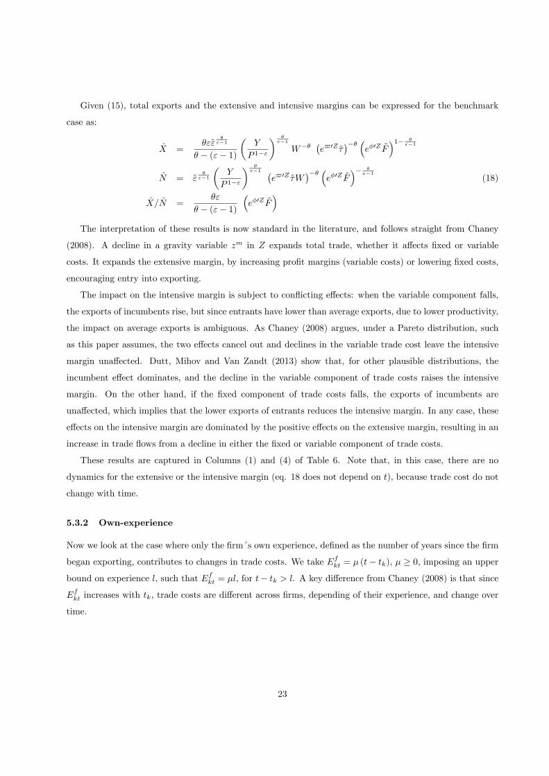
Given (15), total exports and the extensive and intensive margins can be expressed for the benchmark
case as:
�X =�"~"
�"�1
� � ("� 1)
�Y
P 1�"
� �"�1
W�� �e$0Z~���� �e�0Z ~F�1� �"�1
�N = ~"�
"�1
�Y
P 1�"
� �"�1 �
e$0Z~�W��� �
e�0Z ~F�� �
"�1(18)
�X=�N =�"
� � ("� 1)
�e�0Z ~F
�The interpretation of these results is now standard in the literature, and follows straight from Chaney
(2008). A decline in a gravity variable zm in Z expands total trade, whether it a¤ects �xed or variable
costs. It expands the extensive margin, by increasing pro�t margins (variable costs) or lowering �xed costs,
encouraging entry into exporting.
The impact on the intensive margin is subject to con�icting e¤ects: when the variable component falls,
the exports of incumbents rise, but since entrants have lower than average exports, due to lower productivity,
the impact on average exports is ambiguous. As Chaney (2008) argues, under a Pareto distribution, such
as this paper assumes, the two e¤ects cancel out and declines in the variable trade cost leave the intensive
margin una¤ected. Dutt, Mihov and Van Zandt (2013) show that, for other plausible distributions, the
incumbent e¤ect dominates, and the decline in the variable component of trade costs raises the intensive
margin. On the other hand, if the �xed component of trade costs falls, the exports of incumbents are
una¤ected, which implies that the lower exports of entrants reduces the intensive margin. In any case, these
e¤ects on the intensive margin are dominated by the positive e¤ects on the extensive margin, resulting in an
increase in trade �ows from a decline in either the �xed or variable component of trade costs.
These results are captured in Columns (1) and (4) of Table 6. Note that, in this case, there are no
dynamics for the extensive or the intensive margin (eq. 18 does not depend on t), because trade cost do not
change with time.
5.3.2 Own-experience
Now we look at the case where only the �rm´s own experience, de�ned as the number of years since the �rm
began exporting, contributes to changes in trade costs. We take Efkt = � (t� tk), � � 0, imposing an upper
bound on experience l, such that Efkt = �l, for t� tk > l. A key di¤erence from Chaney (2008) is that since
Efkt increases with tk, trade costs are di¤erent across �rms, depending of their experience, and change over
time.
23

It is natural to assume that the �rm internalizes the impact of its entry decision. In these circumstances,
we obtain
Proposition 2 When only own-experience matters, all �rms with productivity above
a � ~" 11�"
�Y
P 1�"
�� 1"�1
W�~�e$0Z
� �~Fe�0Z
� 1"�1�1� �1 + &
� 1"�1
(19)
with:
� =�F�
�F�+�
�1� e�[�F�+�]l
�and & =
("� 1)���("� 1)�����
�e[("�1)�����]l � 1
�0 < (1� �)=(1� &) < 1
enter at t = 0 (pioneers), while the remaining �rms do not enter.
Proof Under Efkt, with experience bounded at �l and @Ekt=@tk = ��, (14) yields
@V
@tk
����Ef
= e��tk��~"� ak~�e$0ZW
�"�1 Y
P 1�"(1 + &) + ~Fe�0Z(1� �)
�where & and � are given above. Note that @V=@tk � 0 implies RktjEf
kt=0� 0. Hence all �rms where
@V=@tk � 0, i.e. those with productivity higher than a, enter at t = 0, while all other �rms do not enter.�
Comparing (15) and (19) we obtain that the threshold of entry is lower when �rms bene�t from their
own-experience (a < �a). Because �rms internalize these dynamic gains, marginal �rms choose to enter as
pioneers, even if they make temporary losses. Eventually, this leads to pro�tability, as trade costs fall, and
these marginal �rms recoup the losses. Hence we can solve for total exports and its composing margins, as
follows
X =�"~"
�"�1
� � ("� 1)
Y
P 1�"j
! �"�1
W�� �~�e$0Z����t��� �1� �1 + &
~Fe�Z�1� �
"�1
N = ~"�
"�1
�Y
P 1�"
� �"�1
W�� �~�e$0Z��� �1� �1 + &
~Fe�0Z�� �
"�1
> �N (20)
X
N=
�"
� � ("� 1)
�1� �1 + &
~Fe�0Z�e����t
The impact of own-experience can be assessed from these expressions. Now, trade costs change through
time, as exporters accumulate experience, rendering the path for exports dynamic. The e¤ect of experience is
related to its impact on trade costs and the potential for anticipation by �rms. First note that, because non-
exporters fail to bene�t from the experience of incumbents, experience accumulated through the passage
of time has no e¤ect on entry, which implies that the extensive margin does not depend on t. Because
24

pro�tability is only a¤ected by presence in the market, there is no point in delaying entry. On the other
hand, the intensive margin and total exports rise with the passage of time and the accumulation of experience
by incumbents, provided experience contributed to lowering variable trade costs. These results are depicted
in Columns (2) and (5) of table 6.
5.3.3 Shared-experience
This section addresses the case where the bene�ts of experience are shared by other �rms, including non-
exporters (through networks of �rms), with spillovers from experience contributing to decline in trade costs,
even for non-incumbents. For simplicity, we take the extreme case where all �rms in o simultaneously and
identically bene�t from the experience of active exporters, and set the experience of �rm k in terms of
industry experience: Eskt = �t, � � 0, reaching an upper bound for t = n.33 Note that this measure of
experience is closer to the one captured in our empirical work, and thus more relevant to interpret our
empirical results.
In such setting, the �rm bene�ts from experience whether or not it is in the market, and trade costs does
not depend on its own actions, namely the time it enters into exports. Hence the incentives for entry of �rm
k change as industry experience evolves, yielding an interesting dynamic of entry depicted in the following
proposition
Proposition 3 When �rms discover through industry experience, all �rms with productivity above
�at � ~"1
1�"
�Y
P 1�"
�� 1"�1
W�~�e$0Z����t
� �~FeZ0���F�t
� 1"�1
(21)
are in the market at time t.
Proof Under Eskt, @Ekt=@tk = 0 and the second term in (14) disappears, yielding @V=@tk = �e��tkRktjDskt=�t
.
The interior solution yields t�(ak), the optimal time of entry for �rm k, where @t�=@ak < 0, i.e. less produc-
tive �rms enter later. Inverting to obtain a(t) we obtain �at, depicting the �rm that enters at time t. Firms
with productivity higher than �a0 enter at time 0, since @V=@tk(tk = 0) < 0.�
When experience is shared, the �rm enters when, and only if, there are non-negative pro�ts. The �rm has
no incentive to take short term losses (as in the case of own-experience), because its gains from experience
do not depend on its own entry decision (but on that of its preceding peers). Hence, at time 0, all �rms
with productivity higher than �a0 enter into exporting as pioneers. Then, the bene�ts of their experience
33Recall that t = 0 is the time when pioneers begin exporting and industry experience starts.
25
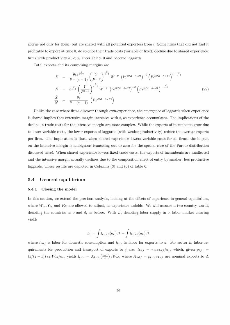
accrue not only for them, but are shared with all potential exporters from i. Some �rms that did not �nd it
pro�table to export at time 0, do so once their trade costs (variable or �xed) decline due to shared experience:
�rms with productivity �at < �a0 enter at t > 0 and become laggards.
Total exports and its composing margins are
�X =�"~"
�"�1
� � ("� 1)
�Y
P 1�"
� �"�1
W�� �~�e$0Z����t��� � ~Fe�0Z��F�t�1� �"�1
�N = ~"�
"�1
�Y
P 1�"
� �"�1
W�� �~�e$0Z����t��� � ~Fe�0Z��F�t�� �"�1
(22)
�X�N
=�"
� � ("� 1)
�~Fe�0Z��F�t
�Unlike the case where �rms discover through own-experience, the emergence of laggards when experience
is shared implies that extensive margin increases with t, as experience accumulates. The implications of the
decline in trade costs for the intensive margin are more complex. While the exports of incumbents grow due
to lower variable costs, the lower exports of laggards (with weaker productivity) reduce the average exports
per �rm. The implication is that, when shared experience lowers variable costs for all �rms, the impact
on the intensive margin is ambiguous (canceling out to zero for the special case of the Pareto distribution
discussed here). When shared experience lowers �xed trade costs, the exports of incumbents are una¤ected
and the intensive margin actually declines due to the composition e¤ect of entry by smaller, less productive
laggards. These results are depicted in Columns (3) and (6) of table 6.
5.4 General equilibrium
5.4.1 Closing the model
In this section, we extend the previous analysis, looking at the e¤ects of experience in general equilibrium,
where Wot; Ydt and Pdt are allowed to adjust, as experience unfolds. We will assume a two-country world,
denoting the countries as o and d, as before. With Lo denoting labor supply in o, labor market clearing
yields
Lo =
Zlko;tg(ak)dk +
Zlkd;tg(ak)dk
where lko;t is labor for domestic consumption and lkd;t is labor for exports to d. For sector k, labor re-
quirements for production and transport of exports to j are: lkd;t = �ktxkd;t=ak, which, given pkj;t =
("=("� 1)) �ktWot=ak, yields lkd;t = Xkd;t�"�1"
�=Wot, where Xkd;t = pkd;txkd;t are nominal exports to d.
26

For domestic production, simply take �kt = 1; to obtain lko;t = Hko;t�"�1"
�=Wot. Substituting in the labor
market clearing condition, we have
WotLo ="� 1"
�ZHko;tg(ak)dk +
ZXkd;tg(ak)dk
�="� 1"
(Dot +Xdt) (23)
where Xdt is given in (17) (and operationalized in eqs. 18, 20 and 22) and Hot is given by
Hot =��"�1"
�"�1� � ("� 1)
�1
Wot
�"�1Yot
P 1�"ot
(24)
A converse equation could be obtained for labor market clearing in d. Meanwhile, total expenditure in
o, on domestic goods and imports, is
Yot =
ZHko;tg(ak)dk +
ZMko;tg(ak)dk
where Mko;t are imports of k of o. We assume that trade is balanced every period, i.e. total imports of o are
equal to total exports to d:RMko;tg(ak)dk =
RXkd;tg(ak)dk. Hence we can express the total expenditure
as34
Yot ="
"� 1WotLo (25)
We can solve for P;X;W;D and Y in both countries, using the expression for P in (9), for X in (17), for
W in (23), for D in (24) and for Y in (25). To close the model, we take Pot = 1 as the numeraire and de�ne
Pdt as the exchange-rate. Now, we assume that countries o and d are identical and focus on the symmetric
equilibrium. Hence we obtain Pot = Pdt = 1 and all nominal aggregate variables, including the wage, denote
real variables.
5.4.2 Numerical exercise
Despite the simpli�cation of symmetry, an analytical solution to the model cannot be reached, and we move
forward with a numerical exercise. The exercise simulates the e¤ect of experience following the event that
starts trade between the two symmetric countries. It assumes that the impact of experience unfolds over 20
years after that event, with a parameter value that arises from the empirical analysis in the previous section.
Other parameter values follow standard assumptions in the literature and are presented Table 5. Without
loss of generality we normalize � = � = 1. The Pareto parameter � is set to 4, following Ghironi-Melitz
(2005), and the elasticity of substitution " is set to 2.5. The literature has found various values for this
34Note that total expenditure overestimates GDP, which must exclude payments of �xed costs.
27
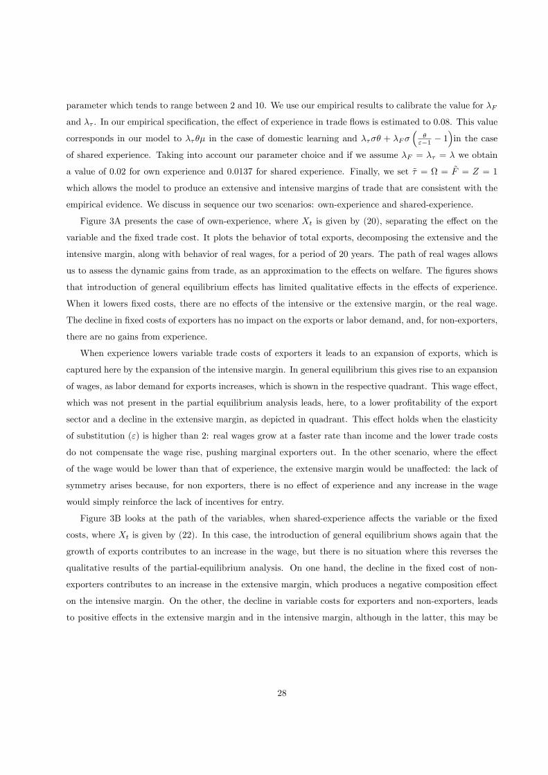
parameter which tends to range between 2 and 10. We use our empirical results to calibrate the value for �F
and �� . In our empirical speci�cation, the e¤ect of experience in trade �ows is estimated to 0.08. This value
corresponds in our model to ���� in the case of domestic learning and ���� + �F��
�"�1 � 1
�in the case
of shared experience. Taking into account our parameter choice and if we assume �F = �� = � we obtain
a value of 0.02 for own experience and 0.0137 for shared experience. Finally, we set ~� = = ~F = Z = 1
which allows the model to produce an extensive and intensive margins of trade that are consistent with the
empirical evidence. We discuss in sequence our two scenarios: own-experience and shared-experience.
Figure 3A presents the case of own-experience, where Xt is given by (20), separating the e¤ect on the
variable and the �xed trade cost. It plots the behavior of total exports, decomposing the extensive and the
intensive margin, along with behavior of real wages, for a period of 20 years. The path of real wages allows
us to assess the dynamic gains from trade, as an approximation to the e¤ects on welfare. The �gures shows
that introduction of general equilibrium e¤ects has limited qualitative e¤ects in the e¤ects of experience.
When it lowers �xed costs, there are no e¤ects of the intensive or the extensive margin, or the real wage.
The decline in �xed costs of exporters has no impact on the exports or labor demand, and, for non-exporters,
there are no gains from experience.
When experience lowers variable trade costs of exporters it leads to an expansion of exports, which is
captured here by the expansion of the intensive margin. In general equilibrium this gives rise to an expansion
of wages, as labor demand for exports increases, which is shown in the respective quadrant. This wage e¤ect,
which was not present in the partial equilibrium analysis leads, here, to a lower pro�tability of the export
sector and a decline in the extensive margin, as depicted in quadrant. This e¤ect holds when the elasticity
of substitution (") is higher than 2: real wages grow at a faster rate than income and the lower trade costs
do not compensate the wage rise, pushing marginal exporters out. In the other scenario, where the e¤ect
of the wage would be lower than that of experience, the extensive margin would be una¤ected: the lack of
symmetry arises because, for non exporters, there is no e¤ect of experience and any increase in the wage
would simply reinforce the lack of incentives for entry.
Figure 3B looks at the path of the variables, when shared-experience a¤ects the variable or the �xed
costs, where Xt is given by (22). In this case, the introduction of general equilibrium shows again that the
growth of exports contributes to an increase in the wage, but there is no situation where this reverses the
qualitative results of the partial-equilibrium analysis. On one hand, the decline in the �xed cost of non-
exporters contributes to an increase in the extensive margin, which produces a negative composition e¤ect
on the intensive margin. On the other, the decline in variable costs for exporters and non-exporters, leads
to positive e¤ects in the extensive margin and in the intensive margin, although in the latter, this may be
28

weakened by the composition e¤ect.3536
5.5 Interpreting the empirical results
Table 6 summarizes our theoretical results, separating the e¤ects of variable and �xed trade costs in each
of three scenarios discussed. The e¤ects of experience depend on whether it lowers variable or �xed trade
costs, as well as the nature of experience. The main conclusion is the con�rmation that experience works to
expand trade. Experience works to expand the extensive margin, only when it is shared by domestic �rms,
as non-exporters enter due to lower trade costs. In the case of own-experience, there is only potential for
non-positive e¤ects, through the extensive margin.
For the intensive margin, the e¤ects of experience depend on the con�icting e¤ects of growth of incumbents
and the entry of small exporters. In the case where own-experience lowers variable costs, experience generates
an unambiguous increase in the intensive margin, because there is no entry of small exporters, who fail to
bene�t from the decline in trade costs. On the other hand, when shared-experience lowers �xed costs, there
is no e¤ect on incumbents and the entry of small exporters lowers the intensive margin.
The results in Table 6 allow us to shed light on the empirical results from the previous section. Now, the
empirical results emerge from a real-life environment that features a linear combination of all the scenarios
in the model (columns in Table 6). Since the various scenarios yield di¤erent, often con�icting, predictions
for the extensive and intensive margins, depending on whether we focus on variable or �xed trade costs or on
own- or shared-experience, the implications for our empirical results on the margins are ambiguous and we
must take a conservative approach in linking empirics and theory. Having said this, we can establish some
key implications from the empirical results obtained.
First, the estimated role of experience on the extensive margin, which captures the impact of country-pair
experience for entry into new HS-6 sectors, implies that shared-experience must play an important role. If
only own-experience mattered, the extensive margin would not adjust (see Figure 3A). Hence, experience
matters not only for the sectors where trade is actually occurring, but also for sectors where trade begins
because trade costs (either �xed or variable ) fall with experience in other sectors. Second,empirically, we
35Our results would also hold in the case of a small open economy that takes prices from the rest of the world as given.
36 In our model, we do not consider multi-product �rms. Although there is a growing literature documenting the importance
of multi-product �rms in international trade, empirical studies are mainly focused on the United States and France due to data
availability. In a recent paper, Bernard et al (2013) study the e¤ect of multi-product �rms on the margin of trade for Belgium
(we should cite this paper: Multi-product exporters and the margins of trade). However, the data are not available for a large
sample of countries and time frame that we analyze in our paper, and we assume that each �rm produces only one di¤erenciated
variety.
29
see that experience expands the intensive margin. This implies that experience, whether it is shared or not,
must impact the variable costs of trade. If only own-experience mattered and it reduced only the �xed costs
of trade, then the intensive margin would not change (see Figure 3A). If shared-experience mattered and
experience reduced only the �xed costs of trade, the intensive margin would decline (Figure 3B). Therefore,
experience must reduce the variable component of trade costs. This is su¢ cient to generate an increase in
the intensive margin either from own-experience or, provided we generalize from the Pareto distribution (see
Dutt, Mihov and Van Zandt 2013), from shared-experience.
6 Conclusion
This paper has addressed the possibility that trade costs, an important determinant of international trade
�ows, may be a¤ected by the experience in exporting. We have established, in the context of the gravity
speci�cation, that experience, proxied by the number of years of positive trade for each country-pairs, works
to expand overall trade and both the intensive and extensive margins of trade. We con�rmed the robustness of
these results, not only to traditional econometric concerns of the gravity literature, but also to measurement
and omitted variables biases associated with our measure of experience. Our within-estimates imply that
one more year of experience reduces trade costs by 2.0%. The role of experience helps explain the dominance
of country-pairs that have been trading with each other for a long time in the growth of world trade, �rst
highlighted in Helpman, Melitz and Rubinstein (2008).
Motivated by the notion that the information barriers and cultural di¤erences that experience helps
bridge are correlated with traditional gravity variables, we have also shown experience�s role in reducing the
impact of traditional trade costs is magni�ed for countries that are separated by geography, lack colonial
links, and with di¤erent legal institutions. The exception is language - the role of experience in facilitating
trade is magni�ed for countries that share a common language.37 Moreover, our results also imply that the
e¤ect of traditional gravity variables, such as distance, decline with experience. This suggests that in periods
where trade emerges for many new country pairs, where bilateral experience is lower, the e¤ect of gravity
variables will be higher. This generate a composition e¤ect that biases upward the estimates of the e¤ects
of gravity variables such as distance, when experience is unaccounted for. This upward bias is a potential
explanation for the persistence of distance, which warrants further investigation.
Due to short time-span of existing �rm-level data, measuring experience accurately at the �rm-level is a
37Kneller and Pisu (2011) survery �rms and �nd something similar - trade costs relating to language di¤erences appear to
increase with the export experience of the �rm.
30
non-trivial task. Therefore, we have focused our analysis at the level of country-pairs. In this case, experience
must be seen as an aggregation of the experience of all the exporter and importer �rms involved in trade
from o to d, including bene�ts that spill over across �rms. Addressing the speci�c e¤ects of experience at the
�rm-level, and the spillovers across �rms remains a challenge for future work, as the time span of �rm-level
datasets expands.
We also addressed the impact of experience for in a dynamic model of international trade with heteroge-
nous �rms. We did this in two settings: �rst, when experience lowers only the trade costs of the exporter, and
second, when it a¤ects the trade costs of the industry. Our setup departs from traditional models, opening
the possibility that trade costs are dynamic and potentially di¤erent across �rms. Our results show that
the e¤ects on the extensive and intensive margins depend on whether experience is shared or not, whether
it a¤ects �xed or variable costs and, to a limited extent, whether we account for general equilibrium e¤ects
on wages or not. In light of the model, our empirical results con�rm that experience reduces variable costs
and is at least partially shared across �rms and industries.
The expansion of trade, due to the e¤ect of experience, implies that the gains from trade are highly
dynamic and that the e¤ect of remoteness (in its multiple dimensions) on trade costs tends to fall with
experience. Given our �nding that the bene�ts from experience tend to be shared among �rms and industries,
the presence of dynamic e¤ects opens the possibility of external e¤ects and the scope for policy: supporting
the entry of early exporters, even temporarily, may lower the trade costs for non-exporters and encourage
entry. Reassessing the role of export-promotion in this light, from the normative and positive perspectives
(e.g. in the East-Asian miracle), remains also a challenge for future research.
References
[1] Albornoz, Facundo, Héctor F. Calvo Pardo, Gregory Corcos, and Emanuel Ornelas. 2012. �Sequential
exporting.�Journal of International Economics, 88(1): 17-31.
[2] Aitken, Brian Gordon H. Hanson, Ann E. Harrison. 1997. �Spillovers, foreign investment, and export
behavior,�Journal of International Economics, 43(1�2), 103-132.
[3] Allen, Treb. 2012. �Information Frictions in Trade.�Working Paper.
[4] Anderson, James E., and Douglas Marcouiller. 2002. �Insecurity and the Pattern of Trade: An Empirical
Investigation.�The Review of Economics and Statistics, 84(2): 342-352.
31

[5] Anderson, James E., and Eric van Wincoop. 2003. �Gravity with Gravitas: A Solution to the Border
Puzzle.�American Economic Review, 93(1): 170-192.
[6] Anderson, James E., and Eric van Wincoop. 2004. �Trade Costs.� Journal of Economic Literature,
42(3): 691-751.
[7] Artopoulos, Alejandro, Daniel Friel, and Juan Carlos Hallak. 2010. �Challenges of Exporting Di¤eren-
tiated Products to Developed Countries: The Case of SME-dominated Sectors in a Semi-Industrialized
Country.�Society for Economic Dynamics 2010 Meeting Papers 1063.
[8] Austin, Peter C. and Lawrence J. Brunner. 2003. �Type I Error In�ation in the Presence of a Ceiling
E¤ect,�The American Statistician, Vol. 57, No. 2, pp. 97-104
[9] Barbieri, Katherine. 2002. The Liberal Illusion: Does Trade Promote Peace? Ann Arbor: University of
Michigan Press
[10] Barbieri, Katherine, and Omar Keshk. 2012. Correlates of War Project Trade Data Set Codebook,
Version 3.0.Online: http://correlatesofwar.org.
[11] Bastos, Paulo and Joana Silva. 2012. �Networks, Firms, and Trade,�Journal of International Economics,
87 (2), 352-364.
[12] Berkowitz, Daniel, Johannes Moenius, and Katharina Pistor. 2006. �Trade, Law, and Product Com-
plexity,�Review of Economics and Statistics, 88:2, 363-373.
[13] Bernard, A. B., Van Beveren, I. and Vandenbussche, H. 2014. �Multi-Product Exporters and the Margins
of Trade.�Japanese Economic Review, 10.1111/jere.12030.
[14] Bernard, Andrew B., J. Bradford Jensen, Stephen J. Redding and Peter K. Schott. 2007. �Firms in
International Trade.�Journal of Economic Perspectives, 21(3): 105-130.
[15] Chaney, Thomas. 2008. �Distorted Gravity: The Intensive and Extensive Margins of International
Trade.�American Economic Review, 98(4): 1707-1721.
[16] Chaney, Thomas. 2014. �The Network Structure of International Trade,�(forthcoming) American Eco-
nomic Review.
[17] Combes, P-P., Lafourcade M. and T. Mayer, 2005. �The Trade Creating E¤ects of Business and Social
Networks: Evidence from France,�Journal of International Economics, 66,1-29.
32

[18] Clerides S., Lach S., Tybout J., 1998. Is learning-by-exporting important? Micro-dynamic evidence
from Colombia, Mexico, and Morocco. Quarterly Journal of Economics 113, 903-47.
[19] Disdier, Anne-Célia, and Keith Head. 2008. �The Puzzling Persistence of the Distance E¤ect on Bilateral
Trade�The Review of Economics and Statistics, 90(1): 37-48.
[20] Dutt, Pushan, and Daniel Traca. 2010. �Corruption and Bilateral Trade Flows: Extortion or Evasion?�
The Review of Economics and Statistics, 92(4): 843-860.
[21] Dutt, Pushan, Ilian Mihov, and Timothy Van Zandt (2013). "The E¤ect of WTO on the Extensive and
Intensive Margins of Trade.�Journal of International Economics, 91(2): 204-219.
[22] Eaton, Jonathan, and Samuel Kortum. 2002. �Technology, Geography, and Trade.�Econometrica, 70(5):
1741-1779.
[23] Eaton, Jonathan, Samuel Kortum, and Francis Kramarz. 2004. �Dissecting Trade: Firms, Industries,
and Export Destinations.�American Economic Review, 94(2): 150-154.
[24] Eaton, Jonathan, Sam Kortum, Brent Neiman, and John Romalis. 2010. �Trade and the Global Reces-
sion.�National Bank of Belgium Working Paper Research 196.
[25] Eaton, J., Eslava, M., Krizan, C., Kugler, M., Tybout, J., 2012. �A search and learning model of export
dynamics,�Working paper.
[26] Egger, Peter H. and Andrea Lassmann. 2012. �The language e¤ect in international trade: A meta-
analysis,�Economics Letters, 116(2), 221-224.
[27] Evenett, Simon, and Anthony Venables. 2002. �Export Growth in Developing Countries: Market Entry
and Bilateral Trade Flows.�www.alexandria.unisg.ch/Publikationen/22177
[28] Flam, Harry, and Hakan Nordström. 2006. �Euro E¤ects on the Intensive and Extensive Margins of
Trade.�CESifo Working Paper Series 1881.
[29] Feenstra, Robert C. and Hiau Looi Kee (2008). �Export Variety and Country Productivity: Estimating
the Monopolistic Competition Model with Endogenous Productivity.� Journal of International Eco-
nomics, 74, 500�518.
[30] Freund, Caroline, and Martha Denisse Pierola. 2010. �Export Entrepreneurs: Evidence from Peru.�
The World Bank Policy Research Working Paper Series 5407.
33
[31] Ghironi, Fabio & Marc J. Melitz, 2005. "International Trade and Macroeconomic Dynamics with Het-
erogeneous Firms," The Quarterly Journal of Economics, 120(3): 865-915.
[32] Glaeser, Edward L., and Andrei Shleifer. 2002. �Legal Origins.�The Quarterly Journal of Economics,
117(4): 1193-1229.
[33] Greif, Avner, 1994. "Cultural Beliefs and the Organization of Society: A Historical and Theoretical
Re�ection on Collectivist and Individualist Societies.�Journal of Political Economy, 102(5): 912-950.
[34] Grossman, G. M., 1998. �Comment� (pp. 29�31), in J. A. Frankel (Ed.), The Regionalization of the
World Economy, Chicago: University of Chicago Press.
[35] Guiso, Luigi, Paola Sapienza, and Luigi Zingales. �Cultural biases in economic exchange?�The Quar-
terly Journal of Economics, 124(3), 1095-1131.
[36] Haveman, Jon, and David Hummels. 2004. �Alternative hypotheses and the volume of trade: the gravity
equation and the extent of specialization.�Canadian Journal of Economics, 37(1): 199-218.
[37] Head, Keith, and John Ries. 1998. �Immigration and Trade Creation: Econometric Evidence from
Canada.�Canadian Journal of Economics, 31(1): 47-62.
[38] Head, Keith, Thierry Mayer, and John Ries. 2010. �The Erosion of Colonial Trade Linkages after
Independence.�Journal of International Economics, 81(1): 1-14.
[39] Head, Keith, and Thierry Mayer. 2013. �Gravity Equations: Workhorse, Toolkit, and Cookbook.�
forthcoming in Handbook of International Economics Vol. 4 (ed. Gopinath, Helpman, and Rogo¤)
[40] Head, Keith and Thierry Mayer. 2013. �What Separates Us? Sources of Resistance to Globalization.�
Canadian Journal of Economics, 46(4): 1196-1231.
[41] Helpman, Elhanan, Marc Melitz, and Yona Rubinstein. 2008. �Estimating Trade Flows: Trading Part-
ners and Trading Volumes.�The Quarterly Journal of Economics, 123(2): 441-487.
[42] Kneller, Richard and Mauro Pisu (2011).�Barriers to Exporting: What are They and Who do They
Matter to?�The World Economy 34(6), 893-930.
[43] Melitz, Marc J. 2003. �The Impact of Trade on Intra-Industry Reallocations and Aggregate Industry
Productivity.�Econometrica, 71(6): 1695-1725.
34
[44] Rauch, James E. 1999. �Networks versus Markets in International Trade.� Journal of International
Economics, 48(1): 7-35.
[45] Rauch, James E., and Vitor Trindade. 2002. �Ethnic Chinese Networks in International Trade.�The
Review of Economics and Statistics, 84(1): 116-130.
[46] Santos Silva, J. M. C., and Silvana Tenreyro. 2006. �The Log of Gravity.�The Review of Economics
and Statistics, 88(4): 641-658.
35
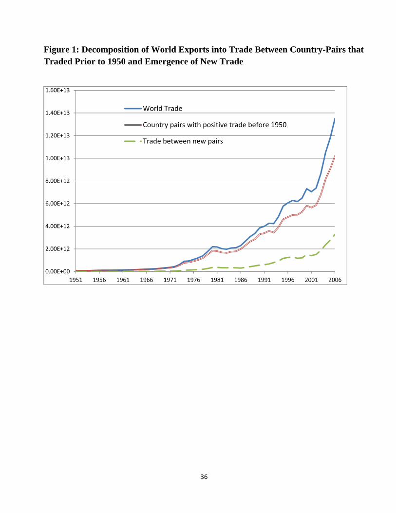
36
Figure 1: Decomposition of World Exports into Trade Between Country-Pairs that Traded Prior to 1950 and Emergence of New Trade
0.00E+00
2.00E+12
4.00E+12
6.00E+12
8.00E+12
1.00E+13
1.20E+13
1.40E+13
1.60E+13
1951 1956 1961 1966 1971 1976 1981 1986 1991 1996 2001 2006
World Trade
Country pairs with positive trade before 1950
Trade between new pairs

37
Figure 2: Distribution of Experience in 2006
0.0
2.0
4.0
6.0
8D
ensi
ty
0 20 40 60Experience

38
Figure 3: Numerical Exercise
3A. Own‐Experience
3B – Shared‐Experience

39
Table 1: Experience-Adjusted Gravity (1) (2) (3) (4) (5) (6) (7) (8) (9) Experience based on DOTS Experience based on COW Country-Pair Dummies Bilateral
exports Extensive margin
Intensive margin
Bilateral exports
Extensive margin
Intensive margin
Bilateral exports
Extensive margin
Intensive margin
Experience 0.060*** 0.029*** 0.031*** 0.032*** 0.014*** 0.018*** 0.084*** 0.041*** 0.043*** (0.001) (0.001) (0.001) (0.001) (0.001) (0.001) (0.008) (0.003) (0.006) Distance -1.217*** -0.819*** -0.398*** -1.267*** -0.870*** -0.397*** (0.018) (0.011) (0.013) (0.020) (0.012) (0.013) Contiguous 0.501*** 0.419*** 0.082 0.351*** 0.324*** 0.027 (0.083) (0.064) (0.053) (0.093) (0.071) (0.053) Colonial relationship 0.895*** 0.604*** 0.291*** 1.032*** 0.655*** 0.376*** (0.092) (0.060) (0.058) (0.103) (0.066) (0.062) Common language 0.397*** 0.455*** -0.058* 0.502*** 0.544*** -0.042 (0.039) (0.023) (0.030) (0.043) (0.025) (0.031) Common law 0.369*** 0.140*** 0.229*** 0.415*** 0.177*** 0.238*** (0.052) (0.029) (0.041) (0.056) (0.031) (0.043) Both in WTO 0.079 0.197*** -0.118*** 0.125* 0.236*** -0.111** 0.172*** 0.219*** -0.047 (0.061) (0.035) (0.044) (0.069) (0.041) (0.051) (0.056) (0.029) (0.047) PTA 0.566*** 0.371*** 0.195*** 0.756*** 0.455*** 0.301*** 0.053 -0.135*** 0.188*** (0.053) (0.033) (0.039) (0.057) (0.035) (0.039) (0.047) (0.024) (0.040) GSP 0.049 0.054** -0.005 0.528*** 0.301*** 0.227*** 0.095 -0.026 0.121 (0.048) (0.024) (0.039) (0.051) (0.026) (0.039) (0.101) (0.036) (0.089) Common currency 0.160 0.018 0.142* 0.033 -0.001 0.035 0.087* -0.083*** 0.170*** (0.120) (0.076) (0.079) (0.126) (0.083) (0.079) (0.047) (0.027) (0.044) Observations 244938 244938 244938 221891 221891 221891 244938 244938 244938 Country-pairs 26089 26089 26089 22202 22202 22202 26089 26089 26089R-squared 0.77 0.84 0.54 0.76 0.84 0.52 0.91 0.96 0.78 Country-year effects Yes Yes Yes Yes Yes Yes Yes Yes YesCountry-pair effects No No No No No No Yes Yes YesStandard errors adjusted for clustering on country-pairs in parentheses;* significant at 10%; ** significant at 5%; *** significant at 1%; All columns include a constant (not shown) .
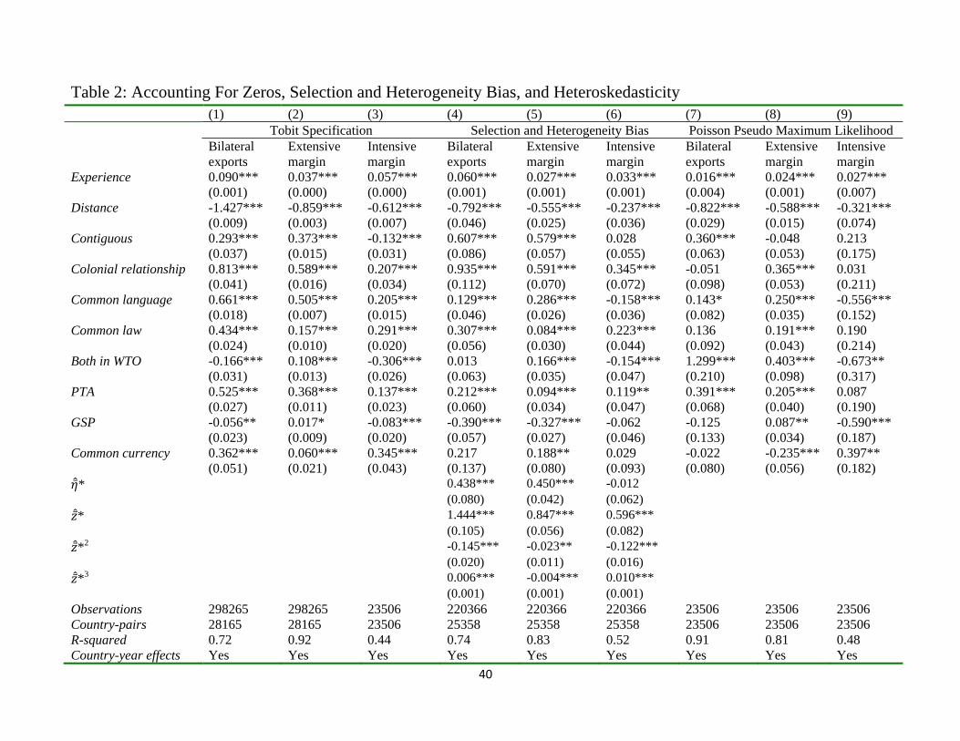
40
Table 2: Accounting For Zeros, Selection and Heterogeneity Bias, and Heteroskedasticity (1) (2) (3) (4) (5) (6) (7) (8) (9) Tobit Specification Selection and Heterogeneity Bias Poisson Pseudo Maximum Likelihood Bilateral
exports Extensive margin
Intensive margin
Bilateral exports
Extensive margin
Intensive margin
Bilateral exports
Extensive margin
Intensive margin
Experience 0.090*** 0.037*** 0.057*** 0.060*** 0.027*** 0.033*** 0.016*** 0.024*** 0.027*** (0.001) (0.000) (0.000) (0.001) (0.001) (0.001) (0.004) (0.001) (0.007) Distance -1.427*** -0.859*** -0.612*** -0.792*** -0.555*** -0.237*** -0.822*** -0.588*** -0.321*** (0.009) (0.003) (0.007) (0.046) (0.025) (0.036) (0.029) (0.015) (0.074) Contiguous 0.293*** 0.373*** -0.132*** 0.607*** 0.579*** 0.028 0.360*** -0.048 0.213 (0.037) (0.015) (0.031) (0.086) (0.057) (0.055) (0.063) (0.053) (0.175) Colonial relationship 0.813*** 0.589*** 0.207*** 0.935*** 0.591*** 0.345*** -0.051 0.365*** 0.031 (0.041) (0.016) (0.034) (0.112) (0.070) (0.072) (0.098) (0.053) (0.211) Common language 0.661*** 0.505*** 0.205*** 0.129*** 0.286*** -0.158*** 0.143* 0.250*** -0.556*** (0.018) (0.007) (0.015) (0.046) (0.026) (0.036) (0.082) (0.035) (0.152) Common law 0.434*** 0.157*** 0.291*** 0.307*** 0.084*** 0.223*** 0.136 0.191*** 0.190 (0.024) (0.010) (0.020) (0.056) (0.030) (0.044) (0.092) (0.043) (0.214) Both in WTO -0.166*** 0.108*** -0.306*** 0.013 0.166*** -0.154*** 1.299*** 0.403*** -0.673** (0.031) (0.013) (0.026) (0.063) (0.035) (0.047) (0.210) (0.098) (0.317) PTA 0.525*** 0.368*** 0.137*** 0.212*** 0.094*** 0.119** 0.391*** 0.205*** 0.087 (0.027) (0.011) (0.023) (0.060) (0.034) (0.047) (0.068) (0.040) (0.190) GSP -0.056** 0.017* -0.083*** -0.390*** -0.327*** -0.062 -0.125 0.087** -0.590*** (0.023) (0.009) (0.020) (0.057) (0.027) (0.046) (0.133) (0.034) (0.187) Common currency 0.362*** 0.060*** 0.345*** 0.217 0.188** 0.029 -0.022 -0.235*** 0.397** (0.051) (0.021) (0.043) (0.137) (0.080) (0.093) (0.080) (0.056) (0.182) * 0.438*** 0.450*** -0.012
(0.080) (0.042) (0.062) * 1.444*** 0.847*** 0.596***
(0.105) (0.056) (0.082) *2 -0.145*** -0.023** -0.122***
(0.020) (0.011) (0.016) *3 0.006*** -0.004*** 0.010***
(0.001) (0.001) (0.001) Observations 298265 298265 23506 220366 220366 220366 23506 23506 23506 Country-pairs 28165 28165 23506 25358 25358 25358 23506 23506 23506 R-squared 0.72 0.92 0.44 0.74 0.83 0.52 0.91 0.81 0.48 Country-year effects Yes Yes Yes Yes Yes Yes Yes Yes Yes

41
Standard errors in parentheses;* significant at 10%; ** significant at 5%; *** significant at 1%; All columns include a constant (not shown) .
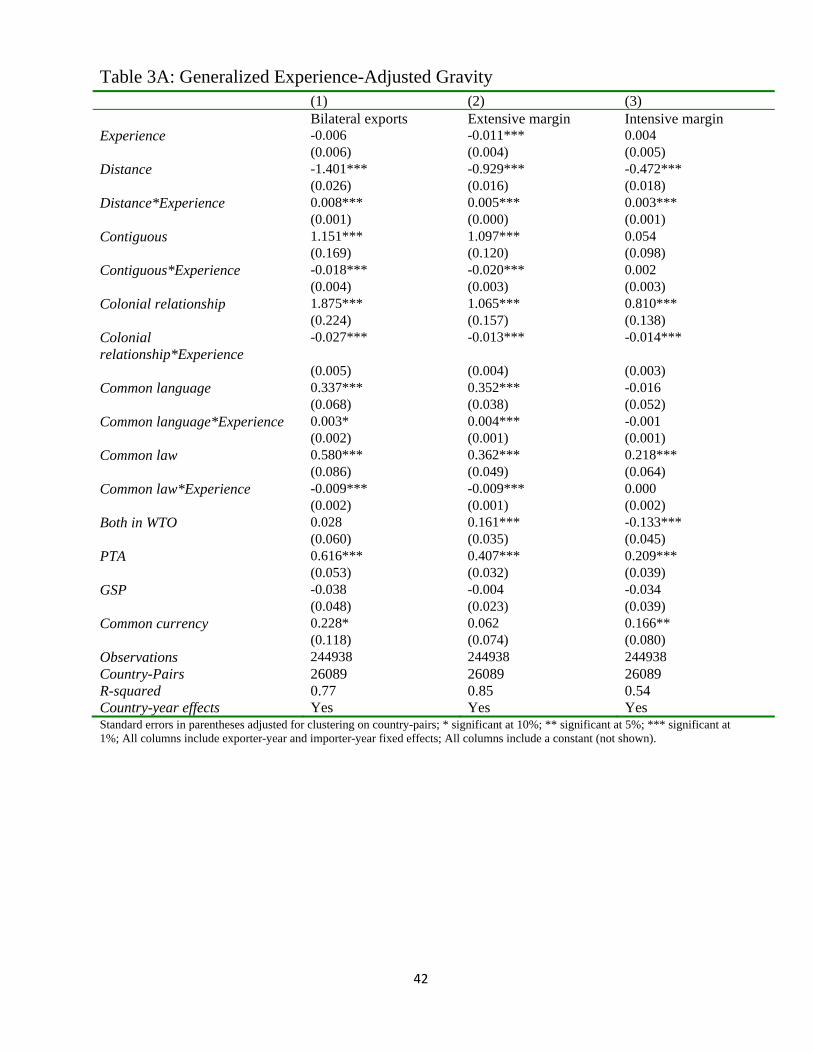
42
Table 3A: Generalized Experience-Adjusted Gravity (1) (2) (3) Bilateral exports Extensive margin Intensive margin Experience -0.006 -0.011*** 0.004 (0.006) (0.004) (0.005) Distance -1.401*** -0.929*** -0.472*** (0.026) (0.016) (0.018) Distance*Experience 0.008*** 0.005*** 0.003*** (0.001) (0.000) (0.001) Contiguous 1.151*** 1.097*** 0.054 (0.169) (0.120) (0.098) Contiguous*Experience -0.018*** -0.020*** 0.002 (0.004) (0.003) (0.003) Colonial relationship 1.875*** 1.065*** 0.810*** (0.224) (0.157) (0.138) Colonial relationship*Experience
-0.027*** -0.013*** -0.014***
(0.005) (0.004) (0.003) Common language 0.337*** 0.352*** -0.016 (0.068) (0.038) (0.052) Common language*Experience 0.003* 0.004*** -0.001 (0.002) (0.001) (0.001) Common law 0.580*** 0.362*** 0.218*** (0.086) (0.049) (0.064) Common law*Experience -0.009*** -0.009*** 0.000 (0.002) (0.001) (0.002) Both in WTO 0.028 0.161*** -0.133*** (0.060) (0.035) (0.045) PTA 0.616*** 0.407*** 0.209*** (0.053) (0.032) (0.039) GSP -0.038 -0.004 -0.034 (0.048) (0.023) (0.039) Common currency 0.228* 0.062 0.166** (0.118) (0.074) (0.080) Observations 244938 244938 244938 Country-Pairs 26089 26089 26089R-squared 0.77 0.85 0.54 Country-year effects Yes Yes Yes Standard errors in parentheses adjusted for clustering on country-pairs; * significant at 10%; ** significant at 5%; *** significant at 1%; All columns include exporter-year and importer-year fixed effects; All columns include a constant (not shown).

43
Table 3B: Marginal Effect of Experience on Bilateral Exports & Bilateral Margins
Bilateral exports Extensive margin Intensive margin Overall 0.059*** 0.029*** 0.031*** (0.001) (0.001) (0.001) Distance (Mean –1 std. dev.) 0.053*** 0.025*** 0.028*** (0.001) (0.001) (0.001) Distance (Mean +1 std. dev.) 0.066*** 0.033*** 0.033*** (0.001) (0.001) (0.001) Contiguity = 0 0.060*** 0.029*** 0.031*** (0.001) (0.001) (0.001) Contiguity = 1 0.042*** 0.010*** 0.032*** (0.004) (0.003) (0.003) Common language =0 0.059*** 0.028*** 0.031*** (0.001) (0.001) (0.001) Common language =1 0.062*** 0.033*** 0.030*** (0.002) (0.001) (0.002) Colonial link = 0 0.060*** 0.029*** 0.031*** (0.001) (0.001) (0.001) Colonial link = 1 0.033*** 0.016*** 0.017*** (0.005) (0.004) (0.003) Common law = 0 0.060*** 0.030*** 0.031*** (0.001) (0.001) (0.001) Common law = 1 0.052*** 0.021*** 0.031*** (0.003) (0.002) (0.002) Observations 244938 244938 244938
Marginal effects are based on Columns (1)-(3) in Table 3A; Standard errors in parentheses; * significant at 10%; ** significant at 5%; *** significant at 1%. Table 3C: Magnitude of Effects for Bilateral Exports
Median Effect
Mean Effect
Minimum Experience (0 years)
First Quartile (8 years)
Median Experience (22 years)
Third Quartile (39 years)
Maximum Experience (58 years)
Distance -1.14 -1.10 -1.401 -1.340 -1.231 -1.100 -0.953 Contiguity 0.52 0.66 1.151 1.005 0.750 0.440 0.093 Common language 0.33 0.39 0.337 0.363 0.409 0.465 0.528 Colonial link 0.84 0.75 1.875 1.660 1.283 0.826 0.315 Common law 0.580 0.510 0.386 0.236 0.069
Median and Mean effect are from structural gravity estimates shown in Head and Mayer (2013a); The next four columns are based on Column (1) in Table 3A

44
Table 4: Accounting for Zeros and Correction for Selection and Heterogeneity Bias (1) (2) (3) (4) (5) (6) Tobit Specification Selection and Heterogeneity Bias Bilateral
exports Extensive margin
Intensive margin
Bilateral exports
Extensive margin
Intensive margin
Experience -0.084*** -0.023*** -0.080*** 0.003 0.007 -0.004 (0.003) (0.001) (0.003) (0.007) (0.004) (0.005) Distance -1.878*** -1.014*** -0.969*** -0.962*** -0.619*** -0.343*** (0.012) (0.005) (0.010) (0.049) (0.026) (0.038) Distance*Experience 0.020*** 0.007*** 0.016*** 0.007*** 0.002*** 0.004*** (0.000) (0.000) (0.000) (0.001) (0.000) (0.001) Contiguous 1.018*** 1.080*** -0.136** 1.097*** 1.005*** 0.092 (0.076) (0.030) (0.064) (0.177) (0.119) (0.098) Contiguous*Experience -0.016*** -0.020*** 0.005*** -0.015*** -0.014*** -0.001 (0.002) (0.001) (0.002) (0.005) (0.003) (0.003) Colonial relationship 2.735*** 1.315*** 1.517*** 1.906*** 1.050*** 0.856*** (0.104) (0.042) (0.088) (0.237) (0.169) (0.143) Colonial relationship*Experience
-0.053*** -0.021*** -0.036*** -0.028*** -0.014*** -0.014***
(0.003) (0.001) (0.002) (0.006) (0.004) (0.004) Common language 0.544*** 0.394*** 0.181*** 0.098 0.180*** -0.083 (0.030) (0.012) (0.025) (0.073) (0.040) (0.057) Common language*Experience
0.007*** 0.005*** 0.002*** 0.003 0.005*** -0.002
(0.001) (0.000) (0.001) (0.002) (0.001) (0.002) Common law 0.715*** 0.350*** 0.419*** 0.452*** 0.248*** 0.204*** (0.037) (0.015) (0.031) (0.089) (0.050) (0.067) Common law*Experience -0.014*** -0.009*** -0.007*** -0.007** -0.007*** 0.000 (0.001) (0.000) (0.001) (0.003) (0.001) (0.002) Both in WTO -0.253*** 0.067*** -0.361*** -0.044 0.140*** -0.183*** (0.031) (0.013) (0.026) (0.062) (0.035) (0.047) PTA 0.660*** 0.421*** 0.235*** 0.280*** 0.127*** 0.153*** (0.027) (0.011) (0.023) (0.060) (0.034) (0.047) GSP -0.248*** -0.060*** -0.219*** -0.423*** -0.339*** -0.085* (0.023) (0.009) (0.020) (0.057) (0.027) (0.046) Common currency 0.543*** 0.125*** 0.486*** 0.222 0.186** 0.036 (0.051) (0.021) (0.043) (0.137) (0.081) (0.093) * 0.438*** 0.450*** -0.012
(0.080) (0.042) (0.062) * 1.444*** 0.847*** 0.596***
(0.105) (0.056) (0.082) *2 -0.145*** -0.023** -0.122***
(0.020) (0.011) (0.016) *3 0.006*** -0.004*** 0.010***
(0.001) (0.001) (0.001) Observations 298265 298265 298265 220366 220366 220366 Country-Pairs 28165 28165 28165 25358 25358 25358 R-squared 0.76 0.84 0.49 0.74 0.83 0.52 Country-year effects Yes Yes Yes Yes Yes YesStandard errors adjusted for clustering on country-pairs in parentheses; * significant at 10%; ** significant at 5%; *** significant at 1%; All columns include exporter-year and importer-year fixed effects; All columns include a constant (not shown).

45
Table 5: Calibrated parameters Parameters Value Definition
1 Own learning 1 Shared learning
1 Impact trade cost ω 1 Impact trade cost
[0.0137,0.02] Learning fixed cost 1 Non-identif trade cost 0.99 Discount factor 2.5 Elasticity Substitution Ω 1 Non-identif trade cost
[0.0137,0.02] Learning variable cost 4 Pareto Parameter 1 Iceberg transport cost 20 Domestic learning 30 Learning spillovers
Table 6: Summary of effects of experience ( )
A. Variable trade costs ( ) B. Fixed trade costs ( ) (1) (2) (3) (4) (5) (6)
Benchmark Own-
Experience Shared-
ExperienceBenchmark
Own-Experience
Shared-Experience
Total Exports
0 > 0 > 0 0 0 > 0
Extensive Margin
0 0 > 0 0 ** > 0
Intensive Margin
0 > 0 * 0 0 < 0
* > 0 under standard distributions (Dutt, Mihov and Van Zandt, 2013); = 0 under Pareto. ** = 0 in partial eq.; < 0 in general eq. when wage effect outweighs experience effect, for
incumbents.


