Download - CFD investigation of a fin keel

CFD investigation of a fin keel
Bachelor of Science Thesis
JAKOB HEIDE
PATRIK LANS
Department of Mechanics
Engineering Mechanics
KTH ROYAL INSITUTE OF TECHNOLOGY
Stockholm, Sweden, 2014


A thesis for the degree of Bachelor of Science
CFD investigation of a fin keel
Jakob Heide
Patrik Lans
Department of Mechanics
KTH ROYAL INSTITUTE OF TECHNOLOGY
Stockholm, Sweden, 2014

CFD investigation of a fin keel
Jakob Heide
Patrik Lans
© Jakob Heide, Patrik Lans, 2014
KTH Royal Institute of Technology
SE-100 44 Stockholm
Sweden
Telephone +46 (0)8-790 60 00
Printed by KTH
Stockholm, Sweden, 2014

iv
Abstract
This thesis aims to help sailboat owners to decide a preferable NACA profile. A CFD
comparison in terms of drag and lift coefficients between two NACA profiles have been
applied on a typical fin keel. Each profile has been computed with different angles of attack to
investigate the impact of small direction changes. ANSYS Fluent 13.0 is used to model the
flow according to RANS k-epsilon model. The conclusion is that NACA65 series gives lower
drag while NACA64 series gives higher lift.
Keywords: sailboat, keel, CFD, RANS, turbulence, NACA profile

v
Sammanfattning
Syftet med det här examensarbetet är att undersöka skillnaderna för olika NACA-kölprofiler
med avseende på tryckkoefficienter Arbetet strävar även efter att ge båtägare en tydligare bild
av en fördelaktig NACA-profil. Varje kölprofil har beräknats med olika anfallsvinklar för att
undersöka effekten av små vinkeländringar. ANSYS Fluent 13.0 har använts för att modellera
flödet enligt k-epsilon-modellen. Slutsatsen är NACA65-serien ger en lägre
motståndskoefficient medan NACA64-serien ger en högre lyftkoefficient.
Nyckelord: segelbåt, köl, CFD, RANS, turbulens, NACA profil

vi
Acknowledgements
The thesis was carried out at KTH Royal Institute of Technology in Stockholm, Sweden. We
would like to thank our supervisor PhD Mireia Altimira on the Department of Mechanics at
KTH for the support throughout the project.
Stockholm, May 2014
Jakob Heide
Patrik Lans

vii

viii
Contents
Nomenclature…………………………………………………………………………………..x
1 Introduction ........................................................................................................................ 1
1.1 Background .................................................................................................................. 1
1.2 Objective ...................................................................................................................... 2
1.3 Methodology ................................................................................................................ 2
1.4 Limitations ................................................................................................................... 2
2 Theory ................................................................................................................................ 3
2.1 Sailing .......................................................................................................................... 3
2.2 Lift and drag ................................................................................................................ 4
2.3 Navier-Stokes equations .............................................................................................. 5
2.4 Turbulence ................................................................................................................... 6
2.5 Pressure coefficient ...................................................................................................... 6
3 Modeling and methods ....................................................................................................... 7
3.1 Background .................................................................................................................. 7
3.2 Geometry ..................................................................................................................... 7
3.2.1 Choice of cases ..................................................................................................... 8
3.3 Computational fluid dynamics ..................................................................................... 9
3.3.1 RANS ................................................................................................................... 9
3.3.2 K-ε model ........................................................................................................... 10
3.3.3 Near wall treatment ............................................................................................ 11
3.4 Meshing ..................................................................................................................... 12
3.4.1 Mesh properties .................................................................................................. 12
3.4.2 Mesh quality ....................................................................................................... 13
3.4.3 Grid variation study ............................................................................................ 14
3.5 Boundary conditions .................................................................................................. 14
3.6 Solution algorithm ..................................................................................................... 16
3.7 Initialization ............................................................................................................... 16
4 Results .............................................................................................................................. 17
4.1 Pressure coefficients on keel ..................................................................................... 18
4.2 Pressure and velocity in 50 % plane .......................................................................... 21
4.3 Tip vortex and turbulent intensity ............................................................................. 25
4.4 Profile comparison ..................................................................................................... 26

ix
4.5 Reliability and validity .............................................................................................. 27
5 Discussion ........................................................................................................................ 28
6 Conclusions ...................................................................................................................... 29
7 Further work ..................................................................................................................... 30
References…………………………………………………………………………………….32
Appendix A…………………………………………………………………………………...33
Appendix B…………………………………………………………………………………...34

x
Nomenclature
Symbols
CD Drag coefficient
CL Lift coefficient
Cp Pressure coefficient
FD Drag force
FL Lift force
Fx,y,z Body force in x-, y- and z-direction
g Acceleration of gravity
k Turbulent kinetic energy
L Characteristic length scale
m Mass
n Normal vector (orthogonal to surface)
p Pressure
Rij Reynolds stress tensor
RM Righting moment
Re Reynolds number
r Refinement ratio
S Planform area
Sij Rate of strain tensor
Sw Wetted surface area
t Time
u+
Non-dimensional velocity
u Flow velocity component in x-direction
ui Instantaneous velocity component in i:th direction
uj Instantaneous velocity component in j:th direction
v Flow velocity

xi
v Flow velocity component in y-direction
V Characteristic velocity scale
w Flow velocity component in z-direction
y+ Non-dimensional wall distance
xi,j Distance in the i or j-direction
Greek symbols
δij Kronecker delta
ε Dissipation rate of turbulent kinetic energy
μ Dynamic viscosity
μt Turbulent viscosity
ν Kinematic viscosity
ρ Density
σij Stress tensor
τ Shear stress
∇ Nabla operator
Abbreviations
CAD Computer-Aided Design
CFD Computational Fluid Dynamics
EWT Enhanced Wall Treatment
FVM Finite Volume Method
ISAF International Sailing Federation
NACA National Advisory Committee for Aeronautics
RANS Reynolds-Averaged Navier-Stokes
SIMPLE Semi-Implicit Method for Pressure-Linked Equations
TKE Turbulent Kinetic Energy

1
1 Introduction
1.1 Background
The performance of sailing yachts is continuously developing. Designers constantly try to find
new strategies to improve their designs both experimentally and numerically by using scaled
models and computer software. For a typical amateur sailor with limited budget and time, the
technical approach of fluid dynamics becomes frightening. The main problem is that, due to
the competitiveness in the industry, most studies are confidential and published papers about
the topic are somewhat unknown to the public. In 2011, Axfors and Tunander investigated
four different keel designs and came up with the conclusion that a bulb integrated keel is the
most suitable for sailboats in terms of performance [1].
Ljungqvist later extended their work and did an optimization of a bulb-integrated keel [2].
Figure 1.1 Fin keel (left) and bulb integrated keel (right)
Since these modern keels are fairly new and therefore less common, it could be helpful for
boat owners to perform a study on a more classic design, i.e. the fin keel. The fin keel was
first introduced in 1891 and it is mounted on most sailboats used today. Even though the trend
for performance sailboats is to use bulb keels, fin keels are still highly competitive. Boat
owners sometimes modify the shape of their keels to increase the performance of their yacht.
This work is usually done by using a plastic filler to achieve a proper shape determined by a
specific template (see Figure 1.2).
The major advantage of the fin keel is its forgiveness in terms of stalling, a phenomenon that
occurs when the flow separates early from the foil, resulting in a reduced lift force. The lift
force is the force perpendicular to the flow direction which is essential in the concept of
sailing towards the wind (upwind). The main inconvenience of the fin design compared to the
bulb keel is that the center of gravity is located closer to the hull and therefore the righting
moment becomes smaller, which results in a lower stability and less capability of using larger
sails.

2
Figure 1.2 Keel optimization using epoxy filler
1.2 Objective
The aim of this project is to investigate how different cross sectional profiles affect the drag
and lift coefficients of a fin keel for different angles of attack. This could be helpful for boat
owners with different preferences where perhaps a highly experienced sailor would prefer
minimum drag and an amateur sailor maximum lift. To set dimensions of a typical fin keel a
competitive one design yacht will be used for this study. The keel of the X-99 sailboat was
developed by x-yachts in 1984 and has since then been produced for over 600 boats1.
The study will provide both X-99 owners and other fin keel owners some insight in how to
best optimize their keel according to NACA airfoil profiles.
1.3 Methodology
Two different NACA profiles are to be numerically examined for varying angles of attack and
the ratio between drag and lift coefficient are to be calculated and analyzed. Ansys CFD
software FLUENT 13.0 will be used for the simulations. Results are presented both in terms
of coefficients (lift and drag) and visually by analysis of the velocity and turbulent fields.
1.4 Limitations
Limitations of this thesis are mainly connected to experimental validation. Since wind and/or
water tunnel testing usually is a complement to CFD, the absence of experimental tests in this
research may decrease the validity of the results. The simulations will be run only for a
constant speed of 6 knots (3 m/s), which is a typical sailboat speed upwind. Additional tests
for other velocities would give a broader insight on the profiles performance. Also, boat
owners might not reshape their keels in perfect accordance with the profiles and a perfectly
smooth surface, which may change the performance significantly. It would also be possible to
take the research one step further using a velocity prediction program for yachts (VPP) to
estimate the practical gains in terms of speed of an optimization. VPP programs are costly and
include a lot of extra work. This thesis focuses on the simulations done by Fluent and the lift
and drag coefficients of the keel, not the actual improvements of the speed while sailing.
1 See x-yachts.com

3
2 Theory
The theory chapter focuses on the background theory of sailing and the concept of flows
around a body.
2.1 Sailing
Sailing is one of the oldest concepts of using the wind energy to create motion. The physics
behind a sailboat heading downwind (in the same direction of the wind) is easy to
comprehend. However, the theory behind a boat heading upwind (towards the wind) involves
a great amount of aerodynamic and hydrodynamic concepts. Easily explained, a sailboat has
two essential components, i.e. the keel and the sails; the former is active in the water and the
latter in the air. The combination of both creates the forward force where both components
work as “wings” creating lift due to varying pressure and velocities around the bodies.
The energy from the wind hits the sails with an angle of attack. Due to the varying
pressure/velocities around the sail, it will work as a wing generating a force perpendicular to
the sail itself (see Figure 2.1). The vector from the sails has one large component sideways
and a smaller component forward. To counteract the boat drifting too much a keel or
centerboard is needed. This wing underwater will, once it is exposed to a flow with an angle
of attack, create both a lift force and a drag force. The sum of the two is shown as Fkeel in
Figure 2.1. Obviously, a relative velocity between the boat and the water is needed for the
keel to operate properly and a small drift off from the course is essential to create the angle of
attack.
Figure 2.1 Showing the forces on a moving sailboat [3]
When course and boat speed are constant, the net lift force is in balance with the drag-force
and dependent on the velocity of the boat through the water.
The design of the keel is an important part of the design process of a sailboat. Parameters like
total weight, total wetted surface and sail area are dependent of each other and the shape of
the keel. A yacht designer looks mainly at the righting moment and the lift performance of the

4
keel. Since the correct righting moment is crucial to counteract the moment created by the
force on the sails, the yacht displacement and center of gravity must be taken into account
when designing the keel. For an amateur sailor willing to experiment with the keel shape the
drag and lift coefficients are of interest, because the displacement and center of gravity are
already fixed.
2.2 Lift and drag
A keel can be compared to a wing of an airplane as a result of the airfoil construction. There
are a lot of similarities regarding the fluid dynamics phenomena that occur. The stagnation
point is the point where the velocity of the fluid is zero, and it takes place when the
streamlines hit the keel. The flow splits at the same point, and continues on the upper
(suction) side and lower (pressure) side. At the same time a pressure difference is created due
to a velocity imbalance between the sides. Basically, this difference is caused by the angle of
attack since the hydrofoils are symmetric. There exist two important dimensionless
coefficients that describe the impact of pressure on the motion of the sailboat. The lift
coefficient expresses a ratio between the lift force and the dynamic forces. The lift force is
orthogonal to the direction of the flow.
21
2
LL
FC
v S
(2.1)
Where FL is the lift force, is the density of the fluid, v is the velocity and S is the planform
area of the object in direction of the lift force LF .
The drag coefficient describes the resistance from an object when a flow comes towards the
body. The drag force is indicated as FD.
21
2
DD
FC
v S
(2.2)
Figure 2.2 The planform area S, defined as the area perpendicular to the frontal area

5
Usually, these two coefficients are combined into a Lift-to-drag ratio, also abbreviated as L/D
– ratio. This parameter is frequently used in aerodynamics but also in hydrodynamics to
describe the efficiency of a studied object concerning its capacity to move forward. The ratio
is a fraction of the quantity of lift caused by the keel divided by the drag which is created by
displacements of the keel within the fluid, i.e. water. Generally for sailboats, a higher L/D-
ratio is preferable because it decreases the drift and induced resistance.
Figure 2.3 Definition of suction side and pressure side around a foil and the directions of the lift and
drag forces. Note: the angle of attack is in reality a lot smaller than in the picture.
2.3 Navier-Stokes equations
The Navier-Stokes equations correspond to the conservation of momentum. The equations are
initially derived from Newton’s second law. One of the main equations to describe the flow
fields is the continuity equation. Water is modelled as an incompressible fluid where the
density is constant and independent of the pressure. Furthermore, water is a Newtonian fluid
with a shear stress linearly proportional to the velocity gradient defined orthogonal from the
shear plane according to the following formula:
ji
ij
j i
uu
x x
(2.3)
where µ is a scalar constant, generally known as the dynamic viscosity. This thesis uses
Einstein notations for all equations except the Navier Stokes equations. The reason for this is
that the overview of the Navier Stokes equation becomes a lot clearer when using standard
notations.
If the fluid is incompressible, which means that the density ρ is unchanged over the entire
domain, the continuity equation can be denoted as follows, where v is the flow velocity:
0 v (2.4)
0u v w
x y z
(2.5)

6
In Cartesian coordinates the Navier-Stokes equations can be formulated as:
2 2 2
2 2 2
1 1x
u u u u p u u uu v w F
t x y z x x y z
(2.6)
2 2 2
2 2 2
1 1y
v v v v p v v vu v w F
t x y z y x y z
(2.7)
2 2 2
2 2 2
1 1z
w w w w p w w wu v w F
t x y z z x y z
(2.8)
The left hand side consists of the total acceleration in a given direction and contains the
unsteady acceleration and the convective acceleration. On the right hand side, the first two
terms describe pressure force and viscous force respectively. The final term displays the body
forces that are acting in the fluid. In the particular case under study, the only body force acting
is gravity.
2.4 Turbulence
Turbulence or turbulent flow consists of chaotic and random variations of all the flow fields.
The Reynolds number (2.9) represents the ratio between inertial forces and viscous forces. At
low Reynolds numbers the flows are laminar, and at higher values, they become turbulent.
The specific values for the change of regime depend on the particular cases.
ReVL
(2.9)
In the previous equation L and V are the characteristic length and velocity of the flow,
respectively. To handle the increasing problem concerning turbulence, the Reynolds
decomposition can be applied on the velocity field. This will be presented more thoroughly in
the next section.
2.5 Pressure coefficient
Pressure coefficients are used to scale the pressure in a domain depending on the freestream
pressure p∞, velocity V∞ and density ρ∞. The pressure coefficient Cp in incompressible flows is
defined as:
21
2
p
p pC
V
(2.10)

7
3 Modeling and methods
3.1 Background
The choice of boat to be investigated is based upon the success of the X-99 class as the
ultimate 10 meters one design keelboat and part of the International Sailing Association
Federation. The yacht X-99 was designed in 1984 by Niels Jeppesen and more than 600 boats
are sold since then. High performance boats like this require strict class rules to limit the
possibilities of modifying the boat to achieve advantages over other racers. The goal is to
create a fair fleet with equal boats and, as a result, rules are set for each component on the
yacht. Among other requirements the keel has, according to the class rules, 5 sections where a
minimum thickness and chord length are defined (see Appendix B).
3.2 Geometry
Yacht designers often use the NACA 6 series due to low drag coefficients and relatively large
lift coefficients. The profiles are obtained through NACA profiles catalogue [4]. The main
difference between NACA64 and NACA65 is the location of the maximum thickness, where
NACA64 has its maximum thickness located at 40 % of total chord length and NACA65 at
45 %. The keel displacement is the same for both designs, and therefore also representing the
same righting moment since their center of gravity will be identical.
The profiles are numerically defined by 5 digits. The first two digits indicate the series type
(e.g. 64 for NACA64). The third digit represents the lift coefficient for 0 degrees angle of
attack and is therefore a measure of the asymmetry of the profile. Since this research only
includes symmetrical sections the third digit will be 0. The last two digits indicate the
maximum thickness over chord length ratio.
Figure 3.1 An example of symmetrical NACA 64/65 profiles with a maximum of 10% thickness-cord
length ratio.

8
Figure 3.2 The different sections defined in the class rules
The investigated case is dependent on specific section requirements in terms of the class rules
for the yacht which limit the options of optimization (see Appendix B for original sketch).
These sections are shown in Figure 3.2 and each section has a minimum allowed chord length
and thickness listed in Table 3.1. The position of the thickest area is non-restricted. The
frontal area and wetted surface should be minimized hence it is beneficial to create a design
which is dimensioned after the minimum allowance of thickness and chord length [5].
Table 3.1 Requirements and parameters for the sections
Section F E D C B A
Z coordinate 0 310 660 1010 1185 1360
Min chord length 1460 1390 1280 1110 980 680
Min thickness 131 137 149 150 140 93
Ratio 0.090 0,099 0,116 0,135 0,143 0,138
Ratio % 9 9,9 11,6 13,5 14,3 13,8
Profile code -009 -010 -012 -015 -015 -015
Figure 3.3 Image of the NACA64 keel drawn in Solid Edge ST5
3.2.1 Choice of cases
The simulations include 8 different cases. Axfors and Tunander (2011) investigated 0, 2 and 4
degrees angle of attack and this thesis will use the same attack angles. Each profile will
therefore be simulated for each of these different angles of attack.

9
3.3 Computational fluid dynamics
The finite volume method, FVM, is a method based on the representation of partial
differential equations as algebraic equations. Basically, the volume integrals that contain a
divergence term in a partial differential equation are converted to surface integrals using the
divergence theorem. Then, these surface integrals are evaluated as fluxes through the surfaces
of each finite volume. The method is easily applicable to all kinds of meshed geometries.
3.3.1 RANS
The three most common approaches to the Navier-Stokes equations are Reynolds-Averaged
Navier-Stokes (RANS), Large Eddy Simulation (LES) and Direct Numerical Simulation
(DNS). While RANS is based on time-averaging all flow fields, LES defines a filter size
above which the scales are exactly resolved. LES gives more accurate results but it requires a
significant larger amount of computer power. DNS is the most accurate since it solves all the
scales of the flow fields, but it also requires the largest amount of computer performance.
Despite its limitations, RANS is still used frequently in several fields due to its competitive
accuracy related to the amount of computer performance it requires.
The Reynolds-Averaged Navier-Stokes equations are derived by first replacing the velocity
and pressure flow variables into a mean and a fluctuating component also called Reynolds
composition. Reynolds decomposition for velocity ui:
'( , , , ) ( , , ) ( , , , )i i iu x y z t u x y z u x y z t (3.1)
By inserting Reynolds decomposition into the flow fields of the Navier-Stokes equations for
an incompressible fluid and then performing time-averaging of the equations it is possible to
derive the Reynolds-Averaged Navier-Stokes equations, for full derivation see [6]:
' 'ji i
j i ij i j
j j j i
uu uu f p u u
x x x x
(3.2)
The last term of the right hand side is called apparent stress, also known as Reynolds stress.
This tensor can be estimated in three different ways, namely the linear eddy viscosity model,
the nonlinear eddy viscosity model and the Reynolds Stress Model. These models can further
be divided into subcategories depending on the model. The most commonly used model is the
linear eddy viscosity, and more specifically the two-equation model of k-epsilon.
Because of its broad usage and the limitations of mixing length model concerning flow
separations, the k-ε model has been adopted in the simulations. The one transport equation
Spallart-Alamaras might only be suitable for certain external flows; otherwise it has more
disadvantages than for the k-ε model. Furthermore, another two-equation model exists,
notably the k-ω model. In this model, ω is the specific rate of dissipation.

10
3.3.2 K-ε model
One of the most common models applied for fluid dynamics problems with turbulent behavior
is the k-ε model. The k-ε model relies on the Boussinesq eddy viscosity assumption which
determines that the Reynolds stress tensor is proportional to the mean strain rate tensor. The
constant of proportionality is called turbulent viscosity.
The eddy viscosity ratio is then defined as;
t
(3.3)
where the upper integer indicates the turbulent viscosity. The major advantage is that this ratio
directly gives a good prediction of the relationship between viscosities which could facilitate
the settings of the inlet boundaries.
This model is based on the transport of turbulent kinetic energy and its dissipation rate:
( )
div( ) div grad 2ti t ij ij
k
kku k S S
t
(3.4)
2
1 2
( )div( ) div grad 2t
i t ij iju C S S Ct k k
(3.5)
k – Turbulence kinetic energy (TKE)
ε – Dissipation rate of the turbulence kinetic energy
In words, these equations can be described as:
The equations incorporate several empirical constants that are changeable. The values of these
constants have been calculated by curve fitting from a wide range of turbulent flows and are;
Cµ = 0.09, σk = 1.00, σε = 1.30, C1ε=1.44, and C2ε = 1.92. These constants have been applied in
the simulations due to their high accuracy concerning airfoils which have been created with a
classical shape.
Finally, Boussinesq relationship is used to compute Reynolds stress:
' ' 2
23
i j t ij iju u S k (3.6)
Rate of change of k or ε + Transport of k or ε by convection = Transport of k or ε by diffusion + Rate
of production of k or ε – Rate of destruction of k or ε

11
3.3.3 Near wall treatment
Wall treatment is the approach of near-wall modelling assumptions for each turbulence
model. As the k-epsilon model is not formulated to model the near wall flow, a damping
function needs to be introduced. Three distinct regions can be defined close to the wall,
namely laminar sublayer, buffer region, and fully-turbulent outer region [7]. It is important to
understand the concept of these layers and how to approach them. There are three different
types of wall treatments available in Fluent; standard wall functions, non-equilibrium wall
functions and enhanced wall treatment (EWT) [8].
The Enhanced Wall Treatment models the velocity u+ with the linear law or the log law
depending on the y+ being above or under 11,63 where the two models meet. The enhanced
wall treatment blends the two laws using a blending function.
For example, y around 15 has a blend coefficient of 0,094 [9] which gives
0,906u u (of viscous sublayer) 0.094 u (of log law)
Where in the viscous sublayer u y and for the log law region 1
ln( )u Ey
.
Figure 3.4 Law of the wall

12
3.4 Meshing
The most appropriate type of grid is dependent on the application; hexahedral meshes are
always preferable since they present less numerical diffusivity, but complex geometries can
only be meshed with tetrahedrons. The convergence of the solution indicates if the mesh is
sufficiently appropriated for this kind of fluid dynamics problem. Due to the simplicity of
refining unstructured grids a tetrahedral mesh is used in this thesis. The mesh parameters are
set the same for all the different cases and a grid variation study is made for the most critical
case. The domain is 23 meters long, 10 meters wide and 10 meters deep. The keel is placed 3
meters from the inlet to represent the hull distance in front of the keel for the yacht.
3.4.1 Mesh properties
The mesh is constructed with a focus on generating a fine mesh around the keel. Face sizing
on the keel is set to 10-4
m with a growth rate of 1,1. Eight inflation layers are set by a first
layer thickness corresponding to a y+ around 15 on the keel. A “keel box” is defined around
the keel as shown in Figure 3.5 with a depth of 2 meters in which the maximum size of the
cells can be 0,075 m3. At the boundary between the “keel box” and the rest of the domain the
cells continue growing with 1,1 growth until they reach a maximum size of 0,5 which is the
maximum cell size.
Figure 3.5 The domain in the X-Z plane with the keel box for the case NACA65 – 4deg
Figure 3.6 The domain in the X-Y plane with the keel box for the case NACA65 – 4deg

13
Figure 3.7 The meshed domain in the X-Y plane (seen from the hull)
Figure 3.8 View of the complete domain (left) and detail of the area around the keel (right)
3.4.2 Mesh quality
There are several ways to measure the mesh quality, but the most frequently used parameters
are aspect ratio, skewness and orthogonal quality. Aspect ratio describes the stretching of the
cell and is calculated as the ratio between the longest and the shortest side of the cell. It is
therefore important to examine the aspect ratio of the cells on locations where the flow
exhibits significant changes. Cells have been plotted by aspect ratios to make sure there are no
critical cells close to the keel.
Another mesh quality parameter is skewness, which defines the asymmetry in a cell and
depends on the angles within the cell (e.g. triangular cells should have 60 degree angles). This
parameter should be below 0,95 for tetrahedral meshes. In this case a few amount of cells
exceed 0,95 and these cells are located on the trailing edge of the keel. High skewness of cells
on the trailing edge of a foil is common to occur when defining inflation layers around the
keel surface. Usually the highly skewed cells on the trailing edge will not affect the solution
but it is important to check for example mass imbalance contours close to the area where
these cells are to ensure that they do not affect the quality of the simulation. Orthogonal

14
quality is computed by the vector from the cell centroid to each of its faces, the corresponding
face area vector, and the vector from the cell centroid to the centroids of each of the adjacent
cells. Orthogonal quality ranges from 0 to 1, where 1 is the most favorable value. There
should not be any cells with an orthogonal quality below 0,01.
Table 3.2 Mesh quality parameters for case NACA65, 4 degrees angle of attack
Parameter Average Min Max
Aspect ratio 3,4128 1,1599 737,37
Skewness 0,2106 0,000021 0,9534
Orthogonal quality 0,8750 0,1063 1
3.4.3 Grid variation study
A grid variation study has been carried out by doing simulations with a coarser mesh and a
finer mesh. The most critical case of the all simulations is assumed to be the NACA65 profile
at 4 degrees angle of attack. This is due to the geometry of the NACA65 profile tends to give
a more critical laminar flow compared to the NACA64. A grid variation study is made by
both increasing and decreasing the number of cells by a factor of 4 2 which is the same as
used in the research by Ljungqvist [2].
Table 3.3 The variation of the grids for the most crucial case
Mesh NACA65_4deg coarse NACA65_4deg NACA65_4deg fine
Cells 5.8 million 6.8 million 8.3 million
Growth rate 1,13 1,1 1,08
3.5 Boundary conditions
The boundary conditions have a vast impact of getting trustworthy results. The k-ε model
affects the boundaries through the specified values of k and ε [10]. The boundary conditions
in Table 3.4 have been used in the computations. Below the following headings, the main sets
will be presented for each geometrical section.
Table 3.4 Boundary conditions in mathematical form
No-slip walls Slip walls Inlet Outlet
u 0iu 0
u
n iu onC stant
0u
n
p 0
p
n 0
p
n 0
p
n
0p
k 0
k
n 0
k
n
onsC tk tan 0
k
n
ε ( )f k 0
n
onsC tant 0
n

15
Figure 3.9 Boundaries and their named selections for both symmetrical (right, 0 degrees) and
asymmetrical (left, 2, 4 degrees) cases
Inlet
At the inlet a constant velocity is set to 6 knots, (i.e. 3 m/s), which is a common speed for
sailboats. Turbulent intensity is set as 5 % because researchers estimate that intensity in open
water [11]. The 5 % level is also generally a commonly used boundary value for open flow
simulation [7]. Turbulent viscosity ratio is set to 10.
Outlet
The outlet is set as an outflow, which means the flow velocity and pressure are not known on
the surface prior to the solution of the flow. No conditions need to be set. Some limitations
with this boundary condition are that it is only valid for incompressible flows where the inlet
is not a pressure inlet (in this case a velocity inlet is used).
Hull
The top side of the domain is the hull. The hull has a no-slip condition and is also defined as a
stationary wall to represent the hull of the sailboat and the turbulence created.
Walls
Due to the solid walls and a high Reynolds number, stationary walls with a specified shear,
known as slip walls, are used in the main calculation. In all cases the solid walls are parallel to
x-direction.
Symmetry
Symmetry planes have been used to simplify the mesh structure for an angle of attack
determined to zero. In the volume around the keel, the inflation command has been used to
increase the resolution of gradients.

16
3.6 Solution algorithm
All simulations use a SIMPLE-algorithm, an acronym for Semi-Implicit Method for Pressure-
Linked Equations, because each case is in a steady state. Approximated velocity fields are
found by the equations of momentum. The pressure gradient term is calculated by the pressure
distribution from the previous iteration. The first iteration is calculated using an initial guess
for the pressure distribution. Afterwards the pressure equation is solved to get the new
pressure distribution and the velocities are adjusted.
The algorithm starts with an initial guess and the following steps are conducted in a loop until
convergence is reached:
1. Solve discretized momentum equations
2. Solve pressure correction equation
3. Correct pressure and velocities
4. Solve all other discretized transport equations
3.7 Initialization
All simulations are initialized with standard initialization computed from the inlet. This gives
a turbulent intensity of 5 % and a turbulent viscosity ratio of 10. These settings give initial
values for k and ε as follows.
Table 3.5 Initial values of transported variables
Transported variable Initial value Unit
k 0.03375 m2/s
2
ε 10.2025 m2/s
3
Under-relaxation is chosen because it is recommended for nonlinear equations (e.g. k- ε
model). A relaxation factor for flow variables of 0.25 is chosen due to increased stability of
the iterations. The required magnitudes of the residuals need to be in accordance with Table
3.6 in order to get a fully converged solution.
Table 3.6 The required residuals calculated as normalized scalars for the simulations
Parameter Continuity k ε x-velocity y-velocity z-velocity
Required
magnitude
10-4
10-5
10-5
10-6
10-6
10-6
A planform area of 1,6623183 m2, a reference velocity of 3 m/s and a reference pressure of 0
Pa are defined for all cases in order to calculate the coefficients for lift, drag and pressure.

17
4 Results
The simulation iterates until the residuals meet the requirements as stated in Table 3.7. Small
fluctuations are noted in some cases but the solution stabilizes as the number of iterations
increase. The solution converges after 2000 iterations for all cases.
Figure 4.1 Example of residuals convergence (NACA64 – 2deg)
The results are presented both graphically and numerically. The horizontal and vertical planes
used to graphically study the flow are defined in Figure 4.2. Drag and lift coefficients are
presented in Table 4.5. Streamlines are attached in Appendix A.
Figure 4.2 Horizontal and vertical planes used in the visual presentations.

18
4.1 Pressure coefficients on keel
Pressure coefficients contours are plotted on the keel surface. For cases where an angle of
attack is defined the suction side is always shown to the left and the pressure side to the right.
0 degrees
The pressure distribution on the surface of the keel is similar for the two profiles. By studying
the graphs it is noted that the pressure coefficent on the keel surface as a function of the
distance downstream is very similar and almost the same as the plotted lines are on top of
each other.
Figure 4.3 Keel pressure coefficients NACA64 (left) and NACA65 (right)
Figure 4.4 Pressure coefficients along the keel surfaces at 25 % and 50 % section of D
Figure 4.5 Pressure coefficients along the keel surfaces at 75 % section of D

19
2 degrees
A tendency of lower pressure on the suction side is displayed for both profiles but mainly in
the lower region of the NACA64 series. By studying the graphs it can be seen that the two
different profiles work with a different range of pressure where the NACA64 series induce a
smaller pressure on both sides. The upper boundary of the graph is the pressure distribution
on the pressure side and the lower the pressure distribution on the suction side. The difference
between the pressure on the suction side and pressure side is however very similar for the two
profiles which indicates that the total lift force should be in the same range.
Figure 4.6 Keel pressure coefficients NACA64
Figure 4.7 Keel pressure coefficients NACA65
Figure 4.8 Pressure coefficients along the keel surfaces at 25 % and 50 % section of D

20
Figure 4.9 Pressure coefficients along the keel surfaces at 75 % section of D
4 degrees
The difference between the suction side and the pressure side is clearly shown as the pressure
side of the keel (the left side of the keel, the figure on the right) inherits a significantly larger
pressure. Also here it is noted that the NACA64 series gives a lower pressure on both sides.
By studying the slopes for the pressure coefficients along the keel surface it can be seen that
the pressure gradient (change of pressure) is largest at 75 % section. This could indicate that
flow separation would appear first at the lower sections of the keel as the attack angle
increases.
Figure 4.10 Keel pressure coefficients NACA64, 4 degrees angles of attack
Figure 4.11 Keel pressure coefficients NACA65, 4 degrees angles of attack

21
Figure 4.12 Pressure coefficients along the keel surfaces at 25 % and 50 % section of D
Figure 4.13 Pressure coefficients along the keel surfaces at 75 % section of D
4.2 Pressure and velocity in 50 % plane
The pressure coefficients indicate that the NACA64 series affects the flow to operate in a
lower pressure relative to the NACA65 series. As shown by the pressure coefficients plotted
on the keel surface the flow close to the keel follow the same direction. The pressure
coefficient of the flow close to the keel surface is lower for the NACA64 series relative the
NACA65 series which is in accordance to the pressure coefficients on the actual surfaces.
By studying the velocities around the keel it is noticeable that the flow on the suction side
travels faster which corresponds to the lower pressure. As the NACA64 series gives a lower
pressure range, the magnitude of the velocity is higher. This is best observed in the case of 2
degrees angle of attack. As the scales of the pressure are constant it is also notable that the
flow around the keel is largely affected by the profiles. Consider the case for 2 and 4 degrees
angle of attack where most of the contours differ even at a distance of around half the chord
length of the keel. The only location where the colors are equal is around the stagnation point
(where the velocity is zero) which is due to the constant free stream velocity defined in both
cases.
22
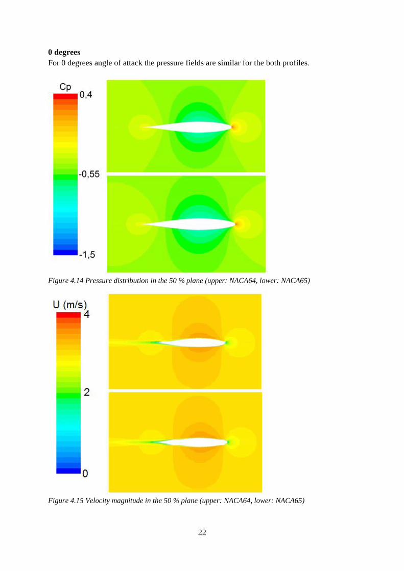
0 degrees
For 0 degrees angle of attack the pressure fields are similar for the both profiles.
Figure 4.14 Pressure distribution in the 50 % plane (upper: NACA64, lower: NACA65)
Figure 4.15 Velocity magnitude in the 50 % plane (upper: NACA64, lower: NACA65)

23
2 degrees
The pressure distribution around the keel is not very similar as the NACA64 keel induces a
lower pressure around itself than the NACA65 keel. This corresponds to the pressure
coefficients plotted on the keel surface in Figure 4.8. As for the stagnation point it is noticed
that it is slightly displaced to the side of the leading edge. As for the velocities it is noted that
the free stream velocity accelerates up to 3,7 m/s at the anterior region of the suction side of
the keel. Because no external energy is added this concludes that the pressure needs to
decrease on this side of the foil.
Figure 4.16 Pressure distribution in the 50 % plane (upper: NACA64, lower: NACA65)
Figure 4.17 Velocities in the 50 % plane (upper: NACA64, lower: NACA65)

24
4 degrees
For 4 degrees the difference in pressure and velocity between the pressure side and the suction
side becomes even more significant. Obviously, the stagnation point is even more displaced to
the side. Moreover, the pressure and velocity differences between the suction and the pressure
side even greater.
Figure 4.18 Pressure distribution in the 50 % plane (upper: NACA64, lower: NACA65)
Figure 4.19 Velocities in the 50 % plane (upper: NACA64, lower: NACA65)

25
4.3 Tip vortex and turbulent intensity
Turbulent intensity levels are plotted in planes situated 0,1, 0,3 and 0,5 meters behind the
keel. The tip vortex can be seen below the keel and it should be noted that it becomes
displaced relatively to the keel for the cases of two and four degrees angles of attack. The tip
vortex is created as spherical forms of a rotating fluid that occurs after an object has generated
lift. All images are shown for the NACA64 series.
Figure 4.20 NACA64 0 degrees, turbulent intensity behind the keel at a distance of 0,1, 0,3 and 0,5 m
Figure 4.21 NACA64 2 degrees turbulent intensity behind the keel at a distance of 0,1, 0,3 and 0,5 m

26
Figure 4.22 NACA64 4 degrees, turbulent intensity behind the keel at a distance of 0,1, 0,3 and 0,5 m
4.4 Profile comparison
The two geometries are compared in Table 4.5 where drag and lift forces are presented
together with their corresponding drag and lift coefficients. It is noted that NACA65 gives
smaller drag coefficients for 2 and 4 degrees. NACA64 gives an almost negligible smaller
drag coefficient for 0 degrees. In terms of lift the NACA64 series has a higher lift coefficient.
The lift over drag ratio is larger for the NACA65 series indicating a better performance for the
yacht.
Table 4.1 Profile comparison
Case N64_0deg N65_0deg N64_2deg N65_2deg N64_4deg N65_4deg
FL (N) 0 0 711,9 711,0 1433,6 1432,3
FD (N) 39,3 39,4 91,7 87,0 127,1 124,0
CL 0 0 0,0953 0,0952 0,1920 0,1918
CD 0,0105 0,0105 0,0123 0,0117 0,0169 0,0166
CL/CD 0 0 7,7653 8,1693 11,3724 11,5519

27
4.5 Reliability and validity
The results of the grid variation study are presented in Table 4.6 and a comparison with
experimental results from the study of Axfors and Tunander (2011) is presented in Table 4.7
[1]. The grid variation study is a mathematical verification of the solution and shows less than
1 % change for the coefficients depending on the mesh quality.
Table 4.2 Grid variation study
Case N65_4deg N65_4deg_Coarse N65_4deg_Fine
Growth rate 1,10 1,13 1,08
Million cells 6,8 5,8 8,3
CL 0,1918 0,1920 0,1917
CD 0,0166 0,01646 0,0166
CL diff % 0 0,1146 - 0,1670
CD diff % 0 0,1508 0,9823
Comparison with the experimental results of another fin keel design shows that the calculated
lift coefficients are deviating by 17 %. The fact that the geometry is slightly different
(NACA63 sections, constant chord length) and no hull is defined might have an impact on the
lift coefficients. Especially the turbulence created near the hull before the flow hits the keel
might affect the lift in the upper region of the keel. This can also be shown in the contours of
pressure coefficients on the keel surface close to the hull (smaller pressure difference between
the suction side and the pressure side).
Table 4.3 Comparison with experimental results by Axfors and Tunander. *Note: Axfors and
Tunander simulated a different geometry consisting of a NACA63 series fin keel without any hull.
Coefficient CD_0deg CD_2deg CD_4deg CL_2deg CL_4deg
Experimental * 0,0108 0,0122 0,0165 0,115 0,228
CFD (Axfors)* - - 0,0170 - 0,253
CFD (X-99) 0,0105 0,0123 0,0169 0,0953 0,1920
Diff % (Axfors)* - - 3,0 - 11,0
Diff % (X-99) -2,5 0,6 2,3 -17,1 -15,8

28
5 Discussion
Classical wing theory has been the approach for this study and the results clearly indicate that
the lift force is created by pressure forces while the drag force is created by both pressure
forces and viscous forces. While the pressure forces are calculated as the pressure integrated
over the area of a surface the viscous forces are due to shear stresses (also integrated over the
surface) close to the wall. Since the k-epsilon model is not appropriate to use for modelling
flow close to a no-slip wall, wall functions are introduced in terms of enhanced wall treatment
which blends the viscous sublayer and the turbulent layer. When the velocity is obtained it is
possible to calculate the shear stress. The results of the forces show that there is a difference
in terms of lift and drag performance between the two designs.
There are two common things which affect the entire solution, errors and uncertainties. Input
uncertainty could have a major impact on the results. The grid variation study indicates that
the lift and drag coefficients vary slightly between three different mesh qualities. The error is
below 1 % which can be seen as a proof of a mathematical verification. By studying the mass
imbalance in the area where a few cells are marginally skewed it can be concluded that these
cells do not affect the result of the simulation.
The experimental comparison for lift coefficients deviates by 17 % which might be seen as a
large error but it is important to state that the geometry differs. The experimental study was
conducted on a NACA63 profile with a constant chord length and no hull. Since the drag
coefficients only differ by 2,5 % it is possible to draw the conclusion that the reference area
used for the calculating the lift and drag coefficients must be defined in a similar manner.
Therefore the difference in terms of lift forces for this thesis and the experimental results
conducted by Axfors and Tunander (2011) could be due to the geometry as the method used is
similar (k-ε and k-ω).
The results correspond in the direction of what an article written by Vacanti says regarding lift
coefficients [12]. It states that the NACA64 series gives a higher lift coefficient at the stall
angle than the NACA65 series. But because the stall angle is at around 11 degrees for the two
profiles it does not say anything about the lift at a normal angle of attack while sailing (11
degrees is significantly higher than 2 and 4 degrees) even though one could assume that the
properties are equal over the whole attack angle range. The results showing that the NACA64
series stands for a higher drag coefficient is however in accordance with the article.
Mesh modifications have been implemented since some areas have been made improperly.
The size of the control volume has been modified during the project due to periodic problems
regarding the mesh structure near the edges. Mesh refinement was necessary along the edges
of the domain due to that the limited viscosity ratio made the solution unstable at times.
Finally, there have been some problems with the remote control function for the computer
used for the simulations. This has regularly caused interruptions and more computational
effort than predicted.

29
6 Conclusions
- The NACA65 profile has a higher lift to drag ratio but larger drag for 0 degrees angle
of attack.
- The grid variation study shows that the mesh quality affects the drag coefficient more
than the lift.
- Comparison with experimental results by Axfors and Tunander (2011) shows that the
lift force deviates more than the drag force since a hull has been meshed.
- A NACA65 series is to prefer if the lift to drag ratio is seen as a performance
parameter.

30
7 Further work
Additional ways to make a deeper study could be by running a velocity prediction program
that includes all parameters (sails, wind, waves, center of gravity, etc.). The hydrodynamic
force model consists of measurements regarding viscous drag, residuary resistance, induced
drag, heel induced drag and added resistance in waves. As a consequence, it could be directly
possible to observe performance differences.

31
References
[1] B. Axfors and H. Tunander , "Investigation of Keel Bulbs for Sailing Yachts," Chalmers
University of Technology, Göteborg, 2011.
[2] K. Ljungqvist, "Shape Optimisation of an Integrated Bulb Keel," Chalmers University of
Technology, Gothenburg, 2011.
[3] B. Anderson, "The physics of sailing," American Institute of Physics, 2008.
[4] ”Public Domain Aeronautical Software,” [Online]. Available:
http://www.pdas.com/profiles.html.
[5] E. Sponberg, ”The Design Ratios,” 2010. [Online]. Available:
http://www.sponbergyachtdesign.com/THE%20DESIGN%20RATIOS.pdf. [Använd
May 2014].
[6] O. Todd, ”A High-Order, Adaptive, Discontinuous Galerkin Finite,” 2004. [Online].
Available: http://raphael.mit.edu/darmofalpubs/Oliver_phd.pdf. [Använd May 2014].
[7] H. Versteeg and W. Malalasekera, An Introduction to computational fluid dynamics,
Second ed., Loughborough: Pearson Education Limited, 2007.
[8] "ANSYS Fluent documentation," [Online]. Available:
http://aerojet.engr.ucdavis.edu/fluenthelp/. [Accessed May 2014].
[9] T. Knopp, "Model-consistent universal wall-functions for RANS turbulence modelling,"
2006. [Online]. Available: http://num.math.uni-
goettingen.de/bail/documents/proceedings/knopp.pdf. [Accessed May 2014].
[10] A. Bakker, "Applied Computational Fluid Dynamics," 2006. [Online]. Available:
http://www.bakker.org/dartmouth06/engs150/06-bound.pdf. [Accessed 2014].
[11] A. Westerhellweg, B. Canadillas and T. Neumann, "Dewi," 2010. [Online]. Available:
http://www.dewi.de/dewi/fileadmin/pdf/publications/Publikations/P10_11.pdf. [Accessed
May 2014].
[12] D. Vacanti, ”Sponberg yacht design,” 2004. [Online]. Available:
http://www.sponbergyachtdesign.com/Keel%20and%20Rudder%20Design.pdf. [Använd
May 2014].

32
Appendix
Appendix A
Pathlines colored by velocity for NACA64 and 2 degrees angle. 50 % plane
Pathlines colored by velocity magnitude for NACA65 and 2 degrees angle. 50 % plane

33
Appendix B


