Figures, Charts, and Tables

Any charts, figures, or tables in your report, whether they are in the main body or the

appendix, must be referenced in the text! Do not put a figure in the report (even one with a

caption) and assume that the reader will be able to figure out the significance of it.

Lab Notebooks

You need to turn in copies of your lab notebook pages with your report. These should be

neatly stapled to the back of your report. See the section below on lab notebooks for the

notebook rubric.

Style

Spelling, grammar, and style are very important in scientific writing. Scientific writing

should be to the point and easy to understand. Unintelligible sentences, poor spelling, and bad

grammar make reports very difficult to read and comprehend. Potential readers will not read

your work and will not learn about any significant results you may have obtained. As such, you

will be penalized for poor spelling, grammar, and syntax. You can lose up to 15 points (25%) off

of your final grade for the following mistakes:

· Major spelling errors: 0.5 pt per error

· Subject/verb agreement issues: 0.5 pt per error

· Punctuation errors (commas, periods, apostrophes, etc.): 0.25 pts per error

· Major grammar errors (incomplete sentences, etc.): 2 pts per error

· Clarity (succinct writing, sentences that flow, proper paragraph structure, etc.): 3 pts per error

The following are some general tips about writing

Write the report in the past tense. You did it already; you are not doing it now and are

not going to do it in the future.

You may write in the first person, using I, we, etc.

Use active voice rather than passive when it makes sense to do so.

Only capitalize proper nouns. Element and chemical names are not proper nouns.

Numbers with units (5 mL, 8.72 ppm) should be written with numerals, regardless of

magnitude. There must be a space between the number and its units (e.g. 5 mL, not 5mL)

except oC and %. Integers less than one hundred or used at the beginning of a sentence

should be spelled out. Numbers that require two words (e.g. 25) have hyphens between

the words (e.g., twenty-five). Decimals should be proceeded by a 0 (e.g 0.5 not .5)

The precision of a number (i.e., significant figures) implies something about the

preparation. For example, “added 5.0 mL of acid and diluted to 100.0 mL” is very

precise – a volumetric pipette was used for the acid and the dilution was made in a

volumetric flask, so it is not necessary to explicitly describe the glassware. In the

contrasting case “added 5 mL of acid and diluted to 100 mL,” the volumes are

approximate and could have been made with graduated cylinders and beakers, and a

description of the glassware is also not required.

The first time you use an abbreviation in the body of the paper, write it out completely

and put the acronym in parenthesis. Then you may use the acronym (e.g., “High

performance liquid chromatography (HPLC) was used for analysis. The HPLC gradient

used was…”)

2

Make sure your language is appropriate to a scientific document. “We got great data” is

not acceptable, nor are terms such as “big” or “small”. If you want to use a word like

“big”, it must be in reference to something else, like “bigger than the EPA limit”, but

“greater than the EPA limit” or “exceeds the EPA limit” is much better phrasing.

PRELAB QUESTIONS

Each experiment has several prelab questions associated with it. Prelab questions are to

be completed before class and given to the TA within the first 15 minutes of class. Answers

turned in after this time will not receive credit!

SAMPLES

Some of the labs you will perform this semester will require you to bring in your own

samples for analysis. These labs are E1: Water Hardness, E5: Zinc in Pet Food, and E7:

Caffeine in Coffee. The necessary samples are a water sample (E1), dog or cat food sample

(E5), and coffee or tea containing caffeine (E7). While there will be other samples for you to

analyze, the results will be more relevant if you are working with your own samples. With the

exception of E7, you will only need to bring in one sample per group. Please coordinate with

your group members to decide who will bring in the samples. You will be docked lab

performance points if you do not collect samples ahead of time. You should document the origin

of the samples (i.e. where they came from or manufacturer) and explain your intellectual

motivation in choosing these samples (why not others?).

LABORATORY NOTEBOOKS

Keeping a good lab notebook is a skill that every scientist must master, regardless of

whether you do research or work for a company. Your lab notebook is the only way you have of

proving what you did and what results you obtained. Becoming proficient at keeping a notebook

is a skill can take a long time, but it will be invaluable in any future work. Your lab notes from

each experiment are worth 20 points apiece, for a total of 160 points (over 10% of your total

course grade).

Lab notebook guidelines

1. The minimum standard for notebooks is that someone who has never taken 4181 can read

your notebook and reproduce what you did.

2. You must write in blue or black ink. Pencil and strange colors are not acceptable. If you

make a mistake, neatly draw a single line through it. You never want to destroy the record of

any data. If you did something wrong, make a note of it and keep going. Do not cross out the

section with your mistakes.

3. You must keep an up-to-date table of contents. You will save much valuable time if you keep

accurate records of where things are.

4. Every page must have a number, the date, and your initials. The date must have the year,

month, and day. Write out the month, e.g. 7 June 2010. 6-7-10 could mean June 7, 2010 or July

3

6, 2010. At the end of the day one of the TAs must initial all the pages for the experiment.

5. You should write an outline of the experiment before you come to lab. This is not a substitute

for your procedure! If you have to perform dilutions or make standards, you should figure out

how to make them before lab. Think about the kinds of data that you are going to collect and

how best to organize it. Doing these things before lab will make the experiment go smoother and

make your notebook much neater.

6. Your lab notebook is a record of what you did, not what the lab manual told you to do.

Procedures that are simply copied from the manual are not acceptable! Recording errors will

often enable you determine why your results are unexpected. The TAs realize that everyone

makes mistakes, and you will not be docked points for making and recording errors.

7. Your procedure should be detailed enough so that someone who has never taken Chem 4181

could repeat the experiment without consulting you. Additionally, when you write your report,

you should be able to write the procedure using only your notebook. It is easy to slack off and

write a poor procedure, but doing this will make it much harder to spot mistakes.

8. You must record all relevant information about the instrument you are using in your

notebook. This includes the make and model, instrument settings, the methods that you used,

and the file names of your data.

9. Include sections for observations and recording any quantitative data.

10. Keep your notebook neat. Write as legibly as possible. If your writing is messy, write big

and skip lines. While the occasional typo or crossed out number is fine, large numbers of

crossed out tables and numbers will look unprofessional. Remember, other people need to be

able to read your lab notebook.

11. Do not leave the lab without all the information (e.g., raw data, plots of spectra etc.) that

were collected by your lab partners. You will need them to prepare your lab report.

LABORATORY NOTEBOOK GRADING RUBRIC: 20 pts total Bookkeeping: 4 pts

Is your table of contents up to date? Are you numbering, dating, and initialing every page? Do

you have a title for your experiment?

Procedure: 8 pts

Is your procedure written in your own words and not simply copied from the lab manual? Is it

detailed enough for someone who has never taken the course to replicate your work?

Data: 8 pts

Is your data reasonably well organized? Do numbers have appropriate units and labels so that an

outsider can understand what the data means?

GOOD LABORATORY TECHNIQUE

Having good laboratory technique is an essential skill for a chemist and will be

invaluable to you in graduate school and especially in industry. While a good GPA can help you

get a job, poor laboratory technique is a surefire way to be unemployed. You will be graded on

your lab performance for the first eight experiments (5 points apiece), and for the student choice

project (35 points).

4

Safety

The most important aspect of any lab is safety. Your safety and the safety of others

always come first!

Safety guidelines

1. All of the safety rules you learned in Gen. Chem. still apply. If anything, they are more

important now as the experiments deal with more dangerous chemicals.

2. You must wear goggles at all times while in the lab. This includes the instrument room!

3. It is a good idea to wear gloves while working with chemicals. While many solvents are not

acutely toxic, long-term exposure can be harmful. Wash your hands whenever you leave the lab.

4. Do not wear gloves when touching the controls of the instruments. It is very easy to

contaminate instruments this way, and decontaminating the instruments is difficult.

5. You must wear closed toed shoes and long pants. Skin-tight pants are not acceptable. Tops

must be at least short sleeved. Long hair must be tied back. If you wear contacts, you should not

wear them in lab. Goggles were designed to fit over glasses.

6. Use the hoods whenever handling volatile solvents or samples that you suspect to be toxic,

especially if the samples could generate dust or fumes. If you are using a hood, turn on the light

and pull the sash as far down as you can. The fume hood will only provide adequate ventilation

when the hood is at least two thirds of the way down.

7. The use of personal electronic devices will not be tolerated while in lab. It is important that

you pay attention to what is happening around you, and it is difficult to do this when wearing

earphones. Personal matters are best dealt with in the hallway. If you do not want to expose your

eyes and skin to dangerous chemicals you certainly should not want to expose your iPhone as

well! The exception to this rule is a personal laptop that may be used to plot data before you

leave the lab to ensure that your calibration curve is linear and that your unknowns are within the

linear region of the calibration curve.

8. Always put a label on all containers (beakers, flasks, etc.) that contains samples or chemicals.

You must include your initials, the date the solution was made, and what the solution

contains. The date must have the day, month, and year. You need to include the concentration

of all species in the container. Additionally, it is a good idea to include the pH if the solution in

particularly acidic or basic.

9. Leave your work areas in as good of or better shape than you found it. A failure to clean up

your mess is not only unsafe, but is disrespectful to the other people who work in the lab. Your

TA will dock you lab performance points for leaving your lab area and equipment that you use

(like balances!) a mess. All chemicals should be returned to where you found them, the balances

should be zeroed and the balance doors closed, and all equipment returned to its original location

and condition. Be courteous; we share the lab space with the inorganic lab and physical

chemistry lab.

Making Up Solutions

Chemists have to make up solutions constantly. Think through all the steps you are going

to do before you do them. Never assume that the numbers in the lab manual are correct. While

every effort has been made to have correct instructions for making solutions, you should always

double-check the numbers that someone else has given you. Double-check your calculations to

make sure that your numbers are correct. Pay attention to the solubility of your compound in the

5

solvent you are using. Make sure there are no hazards associated with mixing the chemicals or

take steps to reduce the hazards. To prevent the class stock material from being contaminated,

never pour excess stock material back into the original container or draw out stock using a

pipette. Always practice quantitative transfer when preparing samples and solutions. Make sure

to label any solutions made up! Include your initials, the full date, and what the solution

contains (see item 8 above). When making standards, try to avoid serial dilutions.

Running Standards and Making a Calibration Curve

When you analyze standards, start with the standard with the lowest concentration and

work up the concentration gradient. If you start with the highest concentration standard, you will

run into trouble because significant traces of the standard can remain after analysis,

contaminating more dilute solutions and skewing your results.

Once you have run all your standards, plot the data using Excel or another graphing

program. Verify that the data is linear and determine the linear range. If any points look

suspicious you should rerun them (assuming that you have enough time). Once you have a good

calibration curve (5 points in the linear range), you can run your unknown samples. Make sure

that the samples are all in the linear range and quantitatively dilute any samples that fall outside

this range. Do not dispose of your samples until you have verified that your calibration curve is

acceptable!

Using Instruments

Almost every lab in this course requires the use of instruments. You should record the

instrument manufacturer and model. Instruments made by different companies or made before a

certain date may exhibit certain quirks that may affect your data. You must also include the

instrument settings (wavelength, injection temperature, etc.) and the name and description of the

method used (if applicable). This information must be in your lab notebook!

UNITS

While molarity is the standard unit of concentration in chemistry, it is often not used in

the real world. The units of moles per liter are not intuitive for non-scientists. A more common

way of expressing how much of an analyte is present is to use a ratio of the amount of analyte to

the total amount of sample. The ratios are usually expressed in terms of “part per…” Typical

ratios are part per million (ppm, one part analyte to one million parts sample), part per billion

(ppb, one part analyte to one billion parts sample), and part per trillion (ppt). Part per hundred is

usually expressed as percent (%) and part per thousand is usually expressed as per mil (‰).

(Note: it is best to write out part per thousand to avoid confusion with part per trillion.

When you have a mass-to-mass ratio, you should add an m to the end to indicate that it is

a mass ratio. Common mass-to-mass ratios are

ppmm g component

g sampleppbm

g component

kg sample

Mass-to-mass ratios are commonly used when reporting results for the analysis of solid materials

such as soil samples.

Volume-to-volume ratios are often used by atmospheric scientists when talking about gas

mixtures. They are also used for the analysis of a liquid component in a liquid sample. For

6

instance, to express ppm in a volume-to-volume ratio, the following relationship applies:

ppmvL component

L sample

Note that when expressing volume-to-volume ratios, a "v" is included in the notation.

When dealing with solutions, the mass-to-mass ratio can be changed into a mass-to-

volume ratio by using the solvent’s density. For the preparation of a solution in which water is

the solvent, the above ppm relationship can be simplified to a mass-to-volume ratio by assuming

the density of water is equal to 1 g/mL. Therefore,

solutionL

solutegppb

solutionL

solutemgppm

This notation is commonly used for regulatory purposes.

In all three cases, you must define what the ratio is. Do not say that the analyte

concentration was 5 ppm without first defining the units of ppm. 5 ppmm is very different from

5 ppmv. Additionally, you should always express your final concentration in terms of the

concentration in the sample. For example, suppose that you extract caffeine from coffee. Your

calibration curve will give you the concentration of caffeine in your extract, but you need to

convert this concentration into the concentration of caffeine in your sample. By keeping track of

how you define your concentration ratio, this task will be much easier.

STATISTICS AND UNCERTAINTY

“There are three kinds of lies: lies, damned lies, and statistics.”

-Mark Twain

While it is true that statistics are often used incorrectly, if applied rigorously they are

invaluable to chemists. Many of the “lies” associated with statistics come from a lack of rigor or

a poor application of the tests available.

Precision and Accuracy

Never say “Bad data was obtained.” “Bad” is a vague term and conveys very little

information. “Bad” could mean that the numbers you measured were significantly different from

the known value, which indicates a lack of accuracy. “Bad” could mean that the numbers were

not consistent with each other, which indicates a lack of precision. “Bad” could also mean that

the results were neither accurate nor precise. Accuracy and precision are two very different

problems and the distinction between the two must be made clear when talking about your data.

Precision describes the reproducibility of a result. Precise measurements are clustered

closely together. Imprecise measurements are scattered. Accurate measurements are close to the

true value of something, while inaccurate measurements are far off from the correct value. It is

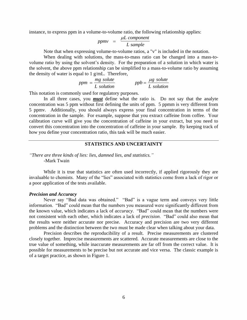
possible for measurements to be precise but not accurate and vice versa. The classic example is

of a target practice, as shown in Figure 1.

7

Figure 1: Accuracy vs. Precision

Figure 1 visually demonstrates the difference between accuracy and precision. The target on the

far right is neither accurate (arrows are not close to the bull’s eye) nor precise (they are widely

scattered) while the far left target is both accurate and precise1.

In the lab, accuracy is established through comparisons with standard reference materials (many

of which are produced by the National Institute of Standards and Technology), or through

comparisons between several methods. It is challenging to determine the accuracy of some

measurements. For example, what is the true concentration of CO in the ambient air today? In

this course, we usually assume that our data are accurate. Thus we are usually more concerned

with how precise our measurements are. The rest of the discussion of statistics and uncertainty

reflects this focus.

Theoretical vs. Experimental Error

Theoretical error is the minimum possible error. In this class, it is the error associated

only with uncertainties in glassware and scale measurements. This is the error that would result

if the lab were run by robots that were capable of measuring out exactly the same quantity every

time they performed a procedure. Experimental error is the actual error that results from doing a

lab. This includes the uncertainties in glassware and scale measurements, but also includes

random error associated with mistakes made in the laboratory (i.e. a volumetric flask filled

slightly too full, some compound dropped on the floor or bench top between when it was

weighed out and added to the flask, slight differences in how a sample was loaded into an

instrument, etc.) Experimental error is almost always much larger than theoretical error because

it includes so many more random factors. In this course, experimental error is calculated by

taking the standard deviation of your measurements and propagating the error from your

calibration curve. Theoretical error is found by propagating the error from glassware and scale

measurements. When reporting error, you must report the larger of the two errors (almost

always experimental error). See Appendix H for the tolerances on glassware and other

laboratory equipment.

Significant Figures and Uncertainty

All final numbers must be reported to the correct number of significant figures. All of

the rules that you learned in Gen. Chem. still apply. Leading zeros are not significant figures

(0.002 has one significant figure), sandwiched zeros are significant (0.00204 has three significant

figures), trailing zeros with a decimal place are significant (0.0020400 has five significant

figures, as does 20000.), and trailing zeros without a decimal place are ambiguous (2000 could

have between one and four significant figures). In addition and subtraction, the number of

significant figures is limited by the value with the least number of decimal places (2.00000 +

Accurate and

precise

Precise but

not accurate

Accurate but

not preciseNeither accurate

nor precise

8

3.00 = 5.00, two decimal places in the final answer; 7.26-6.6=0.66, which rounds to 0.7. In

multiplication and division the number of sig figs in the answer is determined by the term with

the least number of sig figs. The 10x term used in scientific notation has no effect on the number

of sig figs (2*1012

only has one sig fig). If you take the log of a number (like when calculating

the pH), only the numbers after the decimal place in the answer count as significant figures. For

example, if you take the log of 531 (3 sig figs), the answer is 2.725 (three numbers after the

decimal place).

Uncertainties are only reported to one significant figure. Suppose you calculate an

uncertainty of ± 0.54. If you are uncertain about the 5, then you are even less certain about the 4.

However, in many cases in Chem 4181, the number of significant figures will be

determined by the uncertainty associated with that number. In the number 2.34±0.03, the 0.03 is

the uncertainty in the value. The first uncertain figure in the answer (the 4) is the last significant

figure. You cannot have significant digits that are smaller than the uncertainty! While this often

makes it simple to determine the number of significant digits, it can lead to a loss of significant

figures if your error is large. For example, suppose you measure a mercury concentration of

126.1 ppmm with an uncertainty of 75 ppmm (which rounds to 80 ppmm). You can only report

your results as (1.3±0.8) 102 ppmm. Due to the large error, two of the significant figures from

the original answer were lost2.

Mean, Standard Deviation, and Standard Deviation of the Mean

The first two numbers that you should calculate with your data are the mean average and

the standard deviation. You will need at least three measurements of the same thing in order to

calculate a mean and a standard deviation. The mean of a series of measurements is the number

that is the most likely to be the true value. In statistics, this is known as the “expected value.”

The equation for the mean is:

x

x i

i1

n

n (1)

where

x is the mean value, n is the number of measurements, and xi is the ith

measurement. In

other words, to get the mean you add up all of your measurements and divide by the total number

of measurements.

The standard deviation is a measure of how closely data with a Gaussian distribution are

clustered about the mean, i.e., the spread of a set of measurements. We usually make several

measurements, assuming that these samples are representative of the total data population. If the

standard deviation is large, the data are not very closely clustered. If the standard deviation is

very small, the data are all very closely clustered about the mean. The equation for the sample

standard deviation is:

s

(x i x )2

i1

n

n 1 (2)

where s is the standard deviation. For example, the sets {1, 2, 3, 4, 5} and {2.5, 2.75, 3, 3.25,

3.5} both have the same mean of 3, but the first set has a standard deviation of 1.58 and the

second set has a standard deviation of only 0.40. The second set (with the smaller standard

deviation) is clustered much more closely around the mean of 3 than the first set.

Pro

bab

ilit

y o

f

mea

suri

ng

each

x

va

lue

9

http://www.stat.yale.edu/Courses/1997-98/101/normal.htm

Fig. 2: A Gaussian (normal) distribution with mean µ and standard deviation σ. The light grey

shaded area represents ~68% of the area under the curve, while the dark grey shaded area

represents an additional 27% of the area under the curve (i.e., the light and dark grey shaded

areas represent ~95% of the area under the curve).

When averaging data, the standard deviation often can be used as the uncertainty in the final

number3. More measurements would improve our estimate of the population mean, but also take

more time in the lab. What we really want to report is how well our sample mean estimates the

true mean. This statistic is called the standard deviation of the mean (sometimes also called the

standard error of the mean), and is calculated as

√ (3)

Thus it is better to report an average measurement as the mean ± standard deviation of the mean.

Another convention for reporting results of measurements is to report an interval within which

we are (fairly) sure that the mean exists. This “confidence level,” discussed below, is determined

after converting instrumental response to concentration units propagating the related

uncertainties (standard deviation of the means).

Error Propagation and Uncertainty

It is essential that you know how to propagate the uncertainty in your numbers. In

experimental science, almost every number must have an error associated with it. Uncertainty

for a generic function F(x,y,z,…) is calculated by:

eF F

x

2

ex

2

F

y

2

ey

2

F

z

ez

2 ... (4)

where eF is the error in function F, ex is the error associated with variable x, ey is the error

associated with variable y, and ez is the error associated with variable z.

Luckily, you do not have to use this equation every time you want to propagate error.

Formulas for specific, commonly used cases are available. The equations for propagating

uncertainty differ depending on the mathematical operation being used. There are five main

ones that you need to know. You can find these equations (and examples) in Harris and Skoog4.

10

These equations will give you the absolute error. You should also take the time to compute the

relative error, which is the absolute error divided by the value. The relative error is usually

expressed as a percent.

The formula for propagating uncertainty in addition and subtraction (

y x1 x2 or

y x1 x2)

is:

ey ex1

2 ex2

2 (5)

Note that the absolute error will also increase in this case.

The formula for propagating uncertainty in multiplication and division (

y x1 x2 or

y x1

x2

) is:

ey yex1

x1

2

ex2

x2

2

(6)

Note that here the relative error will always increase.

The formula for propagating uncertainty for exponents (

y xa) is:

ey y aex

x

(7)

There are two formulas for propagating uncertainty when taking a logarithm.

For

y ln(x),

ey ex

x, (8)

but for

y log10(x) ,

ey 1

ln(10)

ex

x (9)

When multiplying a number with uncertainty by a constant (such as molar mass), the uncertainty

is:

for

y a x ,

ey aex (10)

You will need to be very familiar with the error propagation formulas. You will have to

propagate your error in all of your lab reports. As was stated earlier, when you take the average

of a set of values, the error in that average is the standard deviation. You would then propagate

that error through your calculations.

Confidence Interval

For your final answer, you should report the error as a confidence interval. The

confidence interval for n measurements is found by

xtxn

tsx (11)

where s is the error and t is the t value for n-1 degrees of freedom at the 95% confidence limit5.

t Tests

A t test is a powerful test that can be used to determine with a specific degree of certainty

whether two values are similar or different. There are two flavors of the t test that you will use

in Chem 4181, and you should be familiar with both of them. To perform a t test, a t value is

calculated (tcalculated) and then compared to the t values listed in a table (ttable, Appendix D).

11

1. The first kind of t-test is used to determine whether a measured value is the same as a known

value. For example, if you did an experiment where you measured the molecular mass of an

element, you would use this type of t test to determine whether your measured value is

significantly different from the true value of the element’s mass. The formula for tcalculated is

tcalculated x known value

sn (12)

where s is the measured standard deviation,

x is the measured mean, and n is the number of

observations. You would then compare the value of tcalcualted to ttable value for n-1 degrees of

freedom at the desired confidence level. If tcalcualted is greater than ttable, then the results are

significantly different.

2. The second type of t test is used to compare replicate measurements. You would use this type

of t test if you measured two samples using the same method or if you measured one sample

using two different methods. For example, if you measured the concentration of ammonia in a

water sample using UV-Vis spectroscopy and with an ammonia selective electrode and you

wanted to see if the two tests gave statistically similar results, this is the t-test you would use.

The formula for tcalculated is

tcalculated x 1 x 2

spooled

n1n2

n1 n2

(13)

where the n’s are the number of measurements and the

x ’s are the measured means. The

formula for spooled is

spooled s1

2(n1 1) s2

2(n2 1)

n1 n2 2 (14)

The one tricky thing about this is that there are n1+n2-2 degrees of freedom, so you need to

compare tcalculated to the ttable value for n1+n2-2 degrees of freedom6.

Analysis of Variance (ANOVA)

An ANOVA test is a complicated version of a t-test. It is used when more than two

samples or sets of data are involved, for example if you were testing three brands of black tea to

see if they had statistically different concentrations of caffeine per serving. The ANOVA test

can tell you whether one is significantly different than the others, but it cannot tell you which one

is different. In order to do that, you must do pair-wise t-tests on the sets of data. However, it can

be a useful time saver because it can tell you that all samples are statistically the same and then

no pair-wise t-tests are required. Excel is capable of performing ANOVA tests7.

Q Test

Sometimes a data point is inconsistent with other data that have been collected. For

example, if you take five readings on the same sample from an instrument, and one is

significantly higher or lower than the other four, you might wish to discard the point. To do this,

you use the Q test. To perform a Q test, arrange the data in order from lowest to highest value

and calculate the gap (the difference between the suspect value and its closest neighboring

value). Then calculate the range (the difference between the highest value and the lowest value,

including the suspect point). Then calculate Qcalculated:

Qcalculated gap

range (15)

12

If Qcalculated is greater than Qtable, then the datum may be discarded. If not, it must be kept. If you

reject a data point, you must include the Q test calculations to justify your decision.

Note: the Q test as described here can only be performed on one-dimensional data; that is you

CANNOT use it to remove a point on a graph which is two-dimensional (contains an x-value and

a y-value). A method for analyzing a suspect point on a calibration curve by performing a Q test

on the residuals is discussed in the section on “Important Terms and Concepts” below8.

How to use Statistics

The following is an example of how you would use the various statistical tests described

above. The first thing that you would do is to make up your standards and then run them on the

instrument. You would then plot the instrument response versus the concentration of the

standards. A quick visual check would be used to check for the linear dynamic range, and then a

line of best fit would be calculated using the points in the LDR. You would then calculate the R2

value for the fit and the residuals. By looking at the R2 value and doing a Q test on the residuals

you can check for anomalous points on the calibration curve and check to see that what you

thought the LDR was is actually the LDR. Once you are satisfied with your calibration curve

you would move on to your samples.

After the sample prep (digestion, filtration, etc.), you would run the samples on the

instrument and obtain the response. You would check the individual responses for each sample

to see if you need to run a Q test to remove bad data. If you have a known value or you ran

several replicates of the same sample you would perform a t test to determine whether the means

are statistically different. You would then average the measurements from a single sample and

run that value through the calibration curve, propagating the error from your measurements and

from the calibration curve through to the end. You would then convert the concentration in the

sample analyzed to the actual sample concentration (if needed)

Important Note: If you do not get high (greater than 0.99) values for R2, do not claim that you

did not get good data, and most importantly, DO NOT PANIC! In many of the experiments, you

will only have a small number of points (around 5) on your calibration curve due to time

restrictions. Additionally, making good calibration standards is an acquired skill, one hopefully

you will have mastered by the end of this course. Remember, a low R2 value or large residuals

do not automatically mean you have bad data. Use the values as a guide to decide whether you

need to remake some of your standards or whether you should include certain points in your

analysis. Finally, the easiest way to get good calibration data is to take the time to make sure

you made everything correctly. If you take the extra time to be careful and make sure that you

have accurate volumes and concentrations, you will find that your data will be significantly

better than if you try to rush through the prep work.

References:

1. Skoog, D. A., Holler, F. J., and Crouch, S. R.

Principles of Instrumental Analysis, Sixth Edition;

Thomson Brooks/Cole: Belmont, CA, 2007, page

967; Harris, D. C. Quantitative Chemical

Analysis, Sixth Edition; W. H. Freeman and

Company: New York, 2003, pages 43-44, 84.

2. Skoog, page 982; Harris, pages 40-42.

3. Skoog, pages 971-973.

4. Skoog, pages 980-982; Harris, pages 44-49.

5. Skoog, page 979; Harris, pages 57-59.

6. Skoog, pages 983-985; Harris, pages 59-62.

7. Skoog, page 985.

8. Harris, page 65.

9. Kirkup, Les. Data Analysis with Excel®;

University Press: Cambridge, 2002, pages 247-

248.

10. Harris, page 83.

11. Kirkup, pages 252-253.

12. http://www.chem.utoronto.ca/coursenotes/analsci/

13

stats/Outliers.html

14

IMPORTANT TERMS AND CONCEPTS

Dark Reading

There is often a small amount of noise associated with the detector that will be present

even when the instrument is not taking any measurements. The easiest way to remove this noise

is to take a dark reading. The detector is isolated from the light source, and the response when

no light hits the detector is measured and subtracted from all subsequent measurements1.

Background

An ideal cell for spectroscopy would be completely transparent at the wavelengths being

used, but this is not always the case. The attenuation due to the cell is measured by inserting an

empty cell into the instrument and taking a reading. Ideally, every cell being used would give

the same response. This is usually the case, but it is something that you may want to check,

especially if the cells are old, were made by different companies, or are made of different

materials. Additionally, the instrument’s wavelength range may be larger than the wavelength

range over which the cell is transparent. The response from the cell is usually very low

compared to the other responses, so you usually do not need to measure it.

Instrument Blank

An instrument blank is used to zero the instrument and is often a cell filled with pure

solvent. This can be used instead of a background1,2

.

Method Blank

An ideal method blank is identical to the sample but is missing the analyte. The method

blank is analyzed in exactly the same way as the samples. The instrument response (not the

concentration!) of the method blank is subtracted from the response of each sample before the

sample concentration is calculated.

The differences between the four types of backgrounds can be easily demonstrated in a

simple UV-Vis experiment. A solid block is inserted into the cuvette holder to take the dark

reading. An empty cuvette is inserted to measure the background. A water-filled cuvette is

inserted to record the instrument blank. Finally, a cuvette filled with all the solution except the

sample is inserted to determine the method blank. In practice you would not have to do all four

of these. You always will need to do at least one of these measurements.

It can be very tempting to skip the blank and simply add a point to the calibration curve at

(0,0). However, you always need to take the time to make a blank. It is difficult to know ahead

of time whether or not there will be signal from the blank, and that signal can impact your

results. In addition, there are several valuable numbers that require a blank to be calculated.

Limit of Detection

The limit of detection (LOD) is the smallest quantity of analyte that gives a response

"significantly different" than the blank. "Significantly different" can be interpreted in many

ways and thus there are many methods used to calculate the limit of detection. A standard way

of determining the LOD is to obtain the instrument response to several (3) blank measurements

and then calculate the average and standard deviation. The LOD is the average blank value plus

15

three times the standard deviation of the blank, as shown in equation 15.

LOD x b 3sb (15)

x b is the average blank reading and sb is the blank standard deviation. Because there are several

other ways of calculating an LOD, you should always specify which one you used and show the

sample calculations. Once you have calculated the LOD, you must convert it to units of

concentration!

If the signal response to a particular sample is below the LOD, you cannot say that

something is there — what appears to be signal may be noise from the background3.

Limit of Quantitation

The limit of quantitation (LOQ) is equal to the average of the blanks plus 10 standard

deviations. This is the point at which signal is strong enough to be measured accurately. If the

response of an unknown is between the LOD and the LOQ, you can say that enough is there to

be detected but not enough to be quantified, i.e. that trace amounts are present3.

Calibration Curve

Calibration curves are one of the most important concepts you will learn about in Chem

4181. Calibration curves are constructed by measuring the response from a number of standards

(5) of known concentrations. The response is then plotted as a function of concentration. If the

data is linear, a line of best fit can be calculated. The equation from the fit allows for the

calculation of the concentration of an unknown. When calculating the line of best fit, you should

never force the line through zero, especially if you have a non-zero value for the blank!

Figure 3: Sample calibration curve.

There are several limitations to calibration curves. First the data must be linear (you can

do non-linear calibration curves but they are hard to use and analyze). Typically, the response

Calibration Curve for X

y = 0.5304x - 0.0002

R2 = 0.9986

0

0.05

0.1

0.15

0.2

0.25

0.3

0.35

0.4

0 0.1 0.2 0.3 0.4 0.5 0.6 0.7 0.8 0.9

Concentration (M)

Resp

on

se (

AU

)

Limit of the LDR

16

will fall off for the higher concentration standards. In solution, this is because the concentration

of analyte molecules is so high that they are interacting with each other instead of with the light.

Below a certain concentration, the response will again often fall off, giving a response of zero for

a range of concentrations. This occurs because there are so few molecules in the solution that

statistically there are not enough in the light path to interact with the light and give a signal. The

range of concentration that follows a straight line is termed the linear dynamic range (LDR)4.

You cannot use points outside of the linear dynamic range when constructing a calibration curve!

The calibration curve is only valid over a given concentration range.

Determining which points should be included in the LDR can be challenging. In the

sample calibration curve shown in Figure 3, there are six points (not counting the blank) on the

line. It is questionable whether the seventh point at 0.7 M is part of the LDR. We describe three

ways to evaluate the line of best fit, and then discuss whether the seventh point on this curve

should be included in the LDR.

There are three ways to verify that the calculated line of best fit is valid, and which points

to include in the LDR. The easiest (but least rigorous) way is to simply look at the data. If you

notice points that are significantly above or below the line or that there is a trend in the data

points (e.g. the first half of the points are above the line and the second half are below the line)

that could indicate that the fit is not very good. It is also easiest to determine the linear dynamic

range using this method. Also, your intercept (after correcting for the blank) should be very

close to zero.

The second way to check your data is to use a quantity called the least-squares parameter

(R2), which a measure of the goodness of the linear fit. The R

2 value is based on the correlation

between x and y and the correlation between y and x. If the correlation is perfect (i.e., all the

points in the calibration curve lie exactly on the line of best fit), the R2 value is 1.000. If the

correlation is less than perfect, the R2 value is lower. Typically, an R

2 value that is close to 1.0 is

interpreted as meaning that the fit to the data is good. However, it is very easy to get a high R2

value for data that does not have a linear relationship. It is even possible to get a high R2 value

for data that is totally random, especially if you do not have many points on your calibration

curve5. In the “real world,” a good R

2 (and thus a good fit) must have a minimum of three 9s.

Thus an R2 of 0.9995 is a good R

2, but an R

2 of 0.991 is not

6. However, obtaining high R

2 values

requires a fair amount of practice with both the instrument and the preparation steps in the

method. In this class you are not going to be expected to obtain perfect values for R2. You will

see R2

values less than 0.9, but do not panic! As long as you can see an apparent trend, the

values are within the linear range, and you calculate the error in your trendline, you can obtain

reasonable results. You do need to be aware of the limitations of R2 and the other ways that you

can validate your results.

A better way of determining goodness of fit is by looking at the residuals. Residuals are

the actual y-value of the data point minus the y-value calculated from the line of best fit at that

particular x-value (i.e., the vertical distance from the point to the line, not the perpendicular

distance). Another way to look at residuals is to look at the standard residuals, where the

residual values have been normalized by the standard deviation of those residuals, so that their

standard deviation is 1. If you plot the residuals versus the x-values, the distribution of the

residuals about zero should be random. If there is a pattern to the residuals, it can indicate that

you do not have a good fit. For example, if the residuals are negative for the first half of your

points and positive for the second half then the data is not linear (it is some form of a quadratic

or exponential).

17

In this class, you will usually be in the linear range, but a case you may encounter is one

where all the residuals save one are negative (or vice versa), or one residual is very large

compared to the others. This case may indicate that you have a bad point on your calibration

curve (which you may have already figured out from looking at the plot). In this case, you have

two options. If the standard residual is greater than 2, it is likely that the point is suspect7. Also,

you may use a Q-test to try to test out that residual and then remove the data point from the

graph8. If you determine that a particular point is bad, you should rerun the sample on the

instrument (assuming that you have time). Even if a suspect point passes the Q test, it is

probably a good idea to rerun that point.

For the calibration curve shown in Figure 3, the line appears to be acceptable as drawn,

but whether the point at 0.7 M should be included in the LDR is questionable. To determine

whether this point is in the linear range, calculate the line of best fit with and without this point.

The quick way to check the point is to compare the R2 values and use the line that gives you the

best R2. The calibration curve in Figure 3 has an R

2 of 0.9986 without the point at 0.7 M and an

R2 of 0.9954 with the point at 0.7 M, indicating that you get a better fit by not including the point

at 0.7 M. A better way to analyze a suspect point is to look at the residuals. If the residual for

the suspect point is the largest residual, then that point is most likely outside of the LDR. In the

end, the determination of which points to include in the LDR is often made operationally, that is,

by looking at the data and making a decision. As much as possible, that decision should be made

on the basis of statistics, but sometimes the choice also depends on intuition.

Let’s continue with our example calibration curve from Figure 3. The residuals for the

seven point calibration curve (which is shown in triangles and does not include the point at 0.7

M) and the eight point calibration curve (which is shown in circles and does include the point at

0.7 M) are shown in Figure 4.

Figure 4: Residuals for the 7 and 8 point calibration curves

If the point at 0.7 M is included in the calibration curve, the magnitude of the residual at

that point (-0.015) is larger than any of the other residuals (the largest residual in the seven point

calibration curve is 0.008), indicating that the point is suspect. Additionally, removing the point

at 0.7 M decreases the residual at 0.6 M from 0.009 to 0.00096. Most of the other residuals in

the seven point curve are also less than the corresponding residuals in the eight point calibration

curve, also indicating that the point at 0.7 M is suspect. Though the residual for the eight fails a

Q test, implying that it should be included in the calibration curve, we would suggest removing

this point. If you have extra time, you should run a standard that is halfway between the last

good point and the suspect point (in this case at 0.65 M). It would also be a good idea to remake

X Variable Residual Plot

-0.016

-0.006

0.004

0.014

0 0.1 0.2 0.3 0.4 0.5 0.6 0.7Res

idu

als

8 point

7 point

18

the standard at 0.4 M and rerun it given that the point at 0.4 M is high for both the seven and

eight point calibration curves.

As a final note on determining the LDR, we present the following text from a “Field

Application Report” for an atomic absorbance spectrometer made by PerkinElmer9:

In section 9.2.2 of the [EPA] method, a procedure for determining the linear

dynamic range (LDR) is described. [The method states, “The LDR should be

determined by analyzing succeedingly higher standard concentrations of the

analyte until the observed analyte concentration is no more than 10% below the

stated concentration of the standard.” In other words, until the observed signal is

10% below the line of best fit.] Standards of 1, 5, 10, 50, 75, 100, 150 and 200

µg/L were analyzed to determine the linear range. Using the lower four standards,

the 100 µg/L standard was within 0.5% of its true value. The 150 µg/L standard

was at -4.7% and the 200 µg/L standard was 9% low. While the 200 µg/L

standard was considered linear by the method (within ±10%), it was found that, if

it or the 150 µg/L standard were included in the calibration, there would be a

large bias effect on the intercept of the calibration curve. Thus, to maintain

accuracy at low levels, the 100 µg/L standard should be considered the upper

linear range. For this study, the sample concentrations were expected to be low

and the calibration consisted of four standards at 1, 5, 10 and 50 µg/L.

In this study, several points were rejected from the LDR because they pulled too hard on

the fit line and caused the intercept to be too large. The best practice for determining the

LDR is to consider carefully the points that might be included in the LDR, find the line of

best fit when including and excluding these points, weigh all of the evidence, and explain

how you made your determination in your report.

Tips for Making and Using a Calibration Curve

When using the calibration curve, it is a good idea to have standards with concentrations

close to those expected for the samples, especially if the samples are at a very low concentration.

Because the leveling off effect discussed above, it can be tricky to determine the concentration of

a sample that gives a low response.

The spacing between the standards should be roughly constant (for example, standards

with concentration of 1 M, 3 M, and 7 M are fine, but standards with concentrations of 0.5 M, 5

M, and 50 M are not).

Samples that give a response greater than the highest point in the linear range must be

diluted and measured again! While calibration curves are useful for analyzing large numbers of

samples, they can fail due to matrix effects (discussed further below).

If you are measuring the concentration of several different analytes in a sample, you will

need separate calibration curves for each sample. Additionally, each analyte will have a different

LOD and LDR. When you report an LOD, LOQ, or LDR, you must specify which analyte and

which instrument you are talking about.

You should be familiar with Excel. A basic tutorial on the features of Excel relevant to

this course is in the appendices of this manual (for both old and new versions of Microsoft

Office), and also at http://www.chem.utoronto.ca/coursenotes/analsci/StatsTutorial/ExcelBasics.html

19

Standard Addition

A matrix effect is a change in the analytical signal due to something other than the

analyte. Matrix effects are often not known before hand, and can be overcome by using a

standard addition calibration curve. A standard addition analysis is performed by measuring the

response of the sample and then adding small amounts of standard to the sample and measuring

the new response. This process is then repeated for each sample. Because the actual sample is

used in all the measurements, any matrix effects that are present will be taken into account. This

technique is very useful because almost every real world sample will have some sort of matrix.

There are two ways of performing standard addition. If your analysis technique does not

consume any sample, then you can perform a standard addition analysis using only one flask.

You begin with a flask containing a known volume of your sample. After you measure the

response, you then spike in a known amount of standard and measure the new response. This

procedure is repeated until you have at least five points. This version of standard addition is not

frequently used because most sampling techniques use up sample and the volume changes (for

example, the atomic absorbance sucks about 5 mL of solution into the instrument per sample and

filling cuvettes for UV-Vis or fluorescence requires several mL per sample). This version could

be used if you make up a 10 mL sample volume and use a 10 µL sample for HPLC; however the

known amount of standard spiked in must also be on the order of microliters so that to first order

it does not affect the volume.

The other way of doing standard addition is more time consuming but is necessary if your

analysis technique uses up some of the sample. This is the version you are most likely to use in

this class. First, a fixed volume of unknown is added to each flask (eg, 5 mL of unknown is

added to each of eight 100 mL volumetric flasks). Then increasing quantities of standard are

added to each flask, as if you were making up regular standards (for example, 0 mL of standard

is added to flask 1, 5 mL is added to flask 2, 10 mL is added to flask 3, etc). Flasks are then

diluted to volume. The result is a series of standards of increasing concentration, but each with a

fixed volume of the unknown. The samples are then analyzed individually10

.

In order to determine the concentration of your unknown, you can plot either response

versus the volume of standard added (the method used in Skoog) or response versus the

concentration of standard added (the method used in Harris) and then find the line of best fit

using the same rules as for a regular calibration curve (samples that are outside the linear range

often cannot be used because it is difficult to dilute them). The method for calculating the

concentration of the unknown is slightly different for each method of graphing, so make sure

your calculations are correct for the type of plot you chose to do!

The concentration of the unknown when using a response versus volume plot is

cx bcs

mVx

(16)

where m and b are the slope and intercept of the linear fit, cs is the concentration of the standard

spiked in, and Vx is the volume of the unknown. The concentration you find with this method is

the actual concentration of your sample11

.

If you use a response versus concentration plot, the concentration of your unknown is

given by

cx b

m (17)

where m and b are, respectively, the slope and intercept of the linear fit. Graphically, this is the

negative of the x-intercept of the linear fit. This concentration is the final concentration of the

20

unknown after it has been diluted. You will need to convert this concentration back to the

original concentration10

.

Unfortunately, when performing a standard addition analysis, each sample must be

analyzed individually. This means you must make and analyze a new set of standards for every

one of your samples, which will be very time-consuming. The great advantage of a normal

calibration curve (i.e. not doing standard addition) is that once the curve has been made, a large

number of samples can be analyzed using that curve. When choosing between using a

calibration curve and doing standard addition, you must decide whether the advantage of

reducing matrix effects outweighs the increased analysis time.

Using Spikes to Determine Efficiency

Another approach to analyzing samples that involve extractions of an analyte is to

calculate the efficiency (sometimes called the percent recovery), which describes how well a

technique measures the analyte. Efficiency is defined as the measured value divided by the

actual (or sometimes theoretical) concentration (Eq. 18).

Efficiency [Measured]

[Actual] (18)

If a technique is 100% efficient, then the final concentration that is calculated will be equal to the

actual concentration in the sample. A technique that is only 50% efficient will give a

concentration that is a factor of two smaller than the actual concentration. An efficiency greater

than 100% is generally considered bad.

To determine the efficiency, a known amount of analyte (the “actual” concentration) is

added (‘spiked’) into a sample (either a blank or a real sample), and then the sample is analyzed.

The measured concentration is the difference between the measured spiked sample concentration

and the unspiked sample concentration. In this course, we will use two techniques in order to

calculate efficiencies: matrix spikes and blank spikes.

When performing a matrix spike, an actual sample is spiked with analyte. The

concentration of the matrix spike is equal to the concentration of the spike plus the concentration

of the sample (Eq. 19).

[Matrix Spike] [Sample] [Spike] (19)

The difference between the measured matrix spike concentration and the sample concentration

will give the measured spike concentration, which is then divided by the calculated

(‘theoretical’) concentration of the spike (the mass of analyte added divided by the total volume

of the matrix spike) as shown in Eq. 20.

][

][] [

Spike

SampleSpikeMatrixEfficiency SpikeMatrix

Where

spikematrixofvolume

volumespikesolutionSpikeSpike

*][][ (20)

Care must be taken when using a matrix spike. The spike concentration should be

roughly equal to the unknown concentration so that the signal from the spike does not drown out

the unknown signal, or vice versa. Additionally, the matrix spike will need to be in the linear

range of the calibration curve in order to use it. Often this means that you must first determine

21

the approximate concentration of the sample and then determine an appropriate spike

concentration.

Despite these challenges, matrix spikes are useful because it is often difficult to replicate

the matrix, and the matrix effects of the sample will be taken into account when using a matrix

spike12

.

Blank spikes are basically a special case of matrix spikes. Blank spikes are made by

taking a method blank and spiking it with a solution containing a known concentration of the

analyte. The blank spike is then run through the same analysis as the other samples. After

calculating the measured concentration, you can obtain the efficiency by dividing the difference

between the measured concentrations of the blank spike and the blank by the calculated spike

concentration, as seen in Eq. 21.

][

][] [

Spike

BlankSpikeBlankEfficiency SpikeBlank

(21)

The spike concentration is the amount of analyte that you spiked into the sample, and the

measured concentration is the concentration obtained from the calibration curve. Blank spikes

are a special case of matrix spikes where the sample concentration is equal to zero.

When calculating efficiencies, the matrix spike cannot be calculated from the instrument

response data or the calculated concentrations of the diluted samples. Instead, you must use the

concentrations of the original samples. In other words, if you had to dilute your matrix spike and

sample, you need to use the calibration curve to calculate the matrix spike and sample

concentrations, account for the dilution, and then use the concentrations of the original sampels

to calculate your efficiencies. You will need to “back track” all the concentrations in order to

account for differences in initial samples.

Once you have your efficiency, you would divide your measured concentration by the

efficiency to obtain the true concentration. When reporting a concentration you should also

report the efficiency. An abnormally low or high efficiency often indicates that you have

interferences present in your sample.

Interferences

Interferences are caused by the presence of other chemical species that either increase or

decrease the signal from the analyte of interest. An abnormally high or low efficiency could

indicate the presence of an interfering species. When interferences are present, you need to

determine a way of the removing the undesired species or switch to a different method.

Positive Interference

A positive interference increases the response of the instrument to a particular

concentration of analyte. For example, the glass membrane for an H+ electrode (such as are

found in pH meters) is also sensitive to Na+ ions. If the pH of a solution is very high (there are

very few H+ ions in the solution) and there is a high concentration of Na

+ ions, the instrument

will read a pH that is too low (it thinks there are more H+ ions in solution than there actually are)

because of the Na+ ions

13.

Negative Interference

A negative interference decreases the response of the instrument to a particular

concentration of analyte. For example, SO4-2

and PO4-3

both create negative interferences with

22

the atomic absorption of Ca+2

, possibly by forming non-volatile salts. Thus if your sample

contains 100 ppm Ca+2

, but also sulfate and phosphate, the response of the AA instrument will be

to report a concentration of Ca+2

of less than 100 ppm14

.

References:

1. Skoog, D. A., Holler, F. J., and Crouch, S. R.

Principles of Instrumental Analysis, Sixth Edition;

Thomson Brooks/Cole: Belmont, CA, 2007, page

159.

2. Harris, D. C. Quantitative Chemical Analysis,

Sixth Edition; W. H. Freeman and Company: New

York, 2003, page 80.

3. Harris, 84-87.

4. Harris, pages 69-71.

5. Kirkup, Les. Data Analysis with Excel®;

University Press: Cambridge, 2002, pages 247-248.

6. Harris, page 83.

7. Kirkup, pages 252-253.

8. http://www.chem.utoronto.ca/coursenotes/analsci/

stats/Outliers.html

9. Hergenreder, R.L. Determination of Arsenic in

Drinking Water by EPA Method 200.9 Using THGA

Graphite Furnace Atomic Absorption, PerkinElmer,

2005, pg. 2, http://www.perkinelmer.com/

CMSResources/Image/44-74357FAR_USEPA2009

ArsenicInDrinkingWater.pdf, accessed 3 Jan. 2012.

10. Harris, pages 87-90.

11. Skoog, pages 13-17.

12. Harris, page 80.

13. Harris, page 312.

14. Harris, page 467

23

WASTE

Learning how to properly manage and dispose of waste is an essential skill for chemists.

Disposing of hazardous waste can cost a significant amount of money and so every effort should

be made to minimize the amount of waste generated. For most of the semester, the TAs will

provide the waste containers for each experiment. However, you will be responsible for all of the

waste generated by your student choice experiment.

How to get rid of waste

1. Select an appropriate waste container. The container material should be compatible with the

chemicals being put into it (for example, do not put bases in glass containers!). For most

purposes a plastic container is fine. The container volume should be at least 10% greater than

the expected waste volume. Every hazardous waste container must be labeled with a hazardous

waste label. Instructions are included in the back of the lab manual. Even though the tag does

not include a space for the date, you should record the date chemicals were first added to the

container. Write the date on a piece of labeling tape or directly on the container. In many places

you can only keep waste for a certain time before it must be disposed of.

2. Separate compounds by class. Keep halogenated and non-halogenated organics separate.

Keep waste contaminated with mercury, lead, or other metals separate from other waste. It is

better to have several small waste containers, each containing a different class of waste, than one

giant waste container with several different kinds of waste. Keep hazardous waste separate from

non-hazardous materials. Solid waste must be kept separate from liquid waste.

3. ALL waste containers must be stored in a secondary waste container. This is usually a large

plastic bin. This is to prevent contamination of the surrounding area in case of leaks. Solid

waste should be double bagged in addition to being placed in a secondary waste container.

HOW TO CONDUCT A GOOD CHEMICAL ANALYSIS EXPERIMENT

In order to conduct an experiment that will yield meaningful results, the first step is to

clearly identify the question or questions that need to be answered. For example, let’s say that

your grandmother lives near an oil refinery in Montana and she tells you that her well water

tastes funny these days. She says, “Since you’re getting a degree in chemistry, can you figure

out why the water tastes funny?” What is the question? You may first formulate a hypothesis:

perhaps run-off from the oil refinery is contaminating the ground water. The question then is

“Are there chemical indicators of the oil refining process within the ground water?” The

question indicates a qualitative chemical analysis problem – “Are there hydrocarbons in ground

water at a detectable level?” If we had asked the question “What is the concentration of benzene

in the ground water?” we would be dealing with a quantitative chemical analysis problem. It is

very important to distinguish between these two types of chemical analyses.

The second step is to consider the best way to acquire a representative sample. In the

above example, you could collect a sample of water from a river that runs through the oil

24

refinery but that wouldn’t necessarily be representative of the well water at your grandmother’s

home. Sample handling is also an important issue since the sample can change as a function of

time after collection.

The next step is to determine the most appropriate technique or techniques required

to address the question. As you will see during this course, some techniques provide a great deal

of qualitative information but are not particularly quantitative. Other techniques are very

quantitative, but do not provide qualitative information. For example, infrared spectroscopy

provides vibrational information about functional groups in a molecule and can sometimes

provide sufficient information for identification of a pure compound. However, it is difficult to

quantify the concentration of a compound within a mixture using infrared absorbance. Another

important issue to address when deciding which technique to use is “Will it be necessary to

separate the analyte from the matrix?” If separation is required, what form would be best?

There is a wide range of separation techniques, including extraction, liquid chromatography, and

gas chromatography. Once the separation technique is chosen, the most appropriate detection

system must be chosen. For example, for liquid chromatography the two most common

detectors are UV-Vis absorbance and fluorescence, each having their own strengths and

weaknesses. Issues such as the required limit of detection, the required linear dynamic range,

sensitivity, and selectivity must be addressed in order to choose the most appropriate detection

system.

Now, what procedure or method will you follow? Is there a standard method (from, say,

the Environmental Protection Agency) that is used to analyze for hydrocarbons? If so, do you

have the necessary equipment or will you have to modify the procedure? If you are not able to

find a standard procedure, you’ll have to develop one. The critical issues are 1) does the sample

need to be “pre-treated” (e.g., extracted, digested, or diluted), 2) what is the possible range of

concentrations, 3) how can standards be prepared to best mimic the sample, 4) calibration of the

instrument, 5) necessary control experiments, and 6) reproducibility. Control experiments

typically include analysis of a “blank”, which is generally comprised of the matrix components

but does not contain the analyte, and analysis of standards from which the signal for a known

concentration is obtained. For quantitative analysis, matrix effects are often addressed by

“spiking” the sample with a known amount of a standard. A spike added to the blank can be

used to determine the extraction efficiency, that is, the fraction of analyte that was removed from

the matrix during sample preparation.

The first eight laboratory experiments in this manual are designed to help you develop the

skills necessary to perform a good chemical analysis experiment. The analytical questions and

techniques have already been chosen and you will be following standard procedures. By paying

attention to how each procedure deals will the six critical issues mentioned above you will

learn to design your own experiment.