field evaluation of center pivot sprinkler irrigation system · center pivot sprinkler irrigation...

1

Final Draft

Field Evaluation of Center Pivot Sprinkler Irrigation Systems

In Michigan

Report Prepared by:

Sabah Almasraf, Jennifer Jury and Steve Miller

Department of Biosystems and Agricultural Engineering

Michigan State University

March 2011

2

Table of Contents

Introduction ..................................................................................................................................... 5

Background and Recent Research ................................................................................................... 7

Objectives ........................................................................................................................................ 8

Study Area and Systems Description ............................................................................................... 8

Methodology and Equations ........................................................................................................... 9

Results and Discussions ................................................................................................................. 12

Fertigation based on Uniformity ................................................................................................... 18

Recommendations......................................................................................................................... 18

Acknowledgements ....................................................................................................................... 23

References ..................................................................................................................................... 24

Appendix A .................................................................................................................................... 25

Appendix B..................................................................................................................................... 30

Appendix C ..................................................................................................................................... 36

3

List of Tables

Table 1. Specifications for the selected field tests. 11

Table 2. Summary of the CU and DU for each test. 13 Table 3. Comparison of Uniformity Coefficients. 15 Table 4. Comparison of water volume applied. 16

Table 5. Potential Application Efficiency (PELQ) 17

Table 6. Number of acres that receive different amounts of Nitrogen in Test 4. 21 Table 7. Soil type analysis for each evaluation field 36

List of Figures

Figure 1. Area covered by each sprinkler increases as the distance from the pivot center

increases. ............................................................................................................................. 6

Figure 2. Map of Tekonsha, Marshall, and Constantine MI. where evaluations tests were

conducted. ........................................................................................................................... 9

Figure 3. Uniformity Coefficient and Distribution Uniformity for all evaluation tests.... 14 Figure 4. Nitrogen distribution based on water applied and sprinkler system uniformity in

test 4. ................................................................................................................................. 19

Figure 5. Nitrogen distribution in test 4 assuming 65 lbs/acre applied over the season by

fertigation in test 4. ........................................................................................................... 20

Figure 6. Graph based on 200 lbs nitrogen application over a season via fertigation in test

4......................................................................................................................................... 20 Figure 7. Nitrogen application was calculated on test 2 with the greatest uniformity rating

(89%) assuming all nitrogen is applied via fertigation (200 lbs. over the season). .......... 21

Figure 8. Rotating Sprays mounted on the lateral of the center pivot. ............................. 25 Figure 9. Catch cups lined up along the edge of the corn crop. ........................................ 25 Figure 10. Measuring water volume from catch cup. ....................................................... 26

Figure 11. Row of cups before irrigation line has passed over. ........................................ 26 Figure 12. Using the Ultra-sonic flow meter to measure flow rate through the system. .. 27 Figure 13. Center pivot with end gun on. ......................................................................... 27

Figure 14. Water leaking from the lateral joint on the center pivot line. .......................... 28 Figure 15. Center pivot irrigation operating. .................................................................... 28 Figure 16. Rotating sprays suspended from the lateral of the center pivot. ...................... 29 Figure 17. End Gun off during the evaluation test............................................................ 29 Figure 18. Water distribution of Test 1. ............................................................................ 30

Figure 19. Water distribution of Test 2. ............................................................................ 30

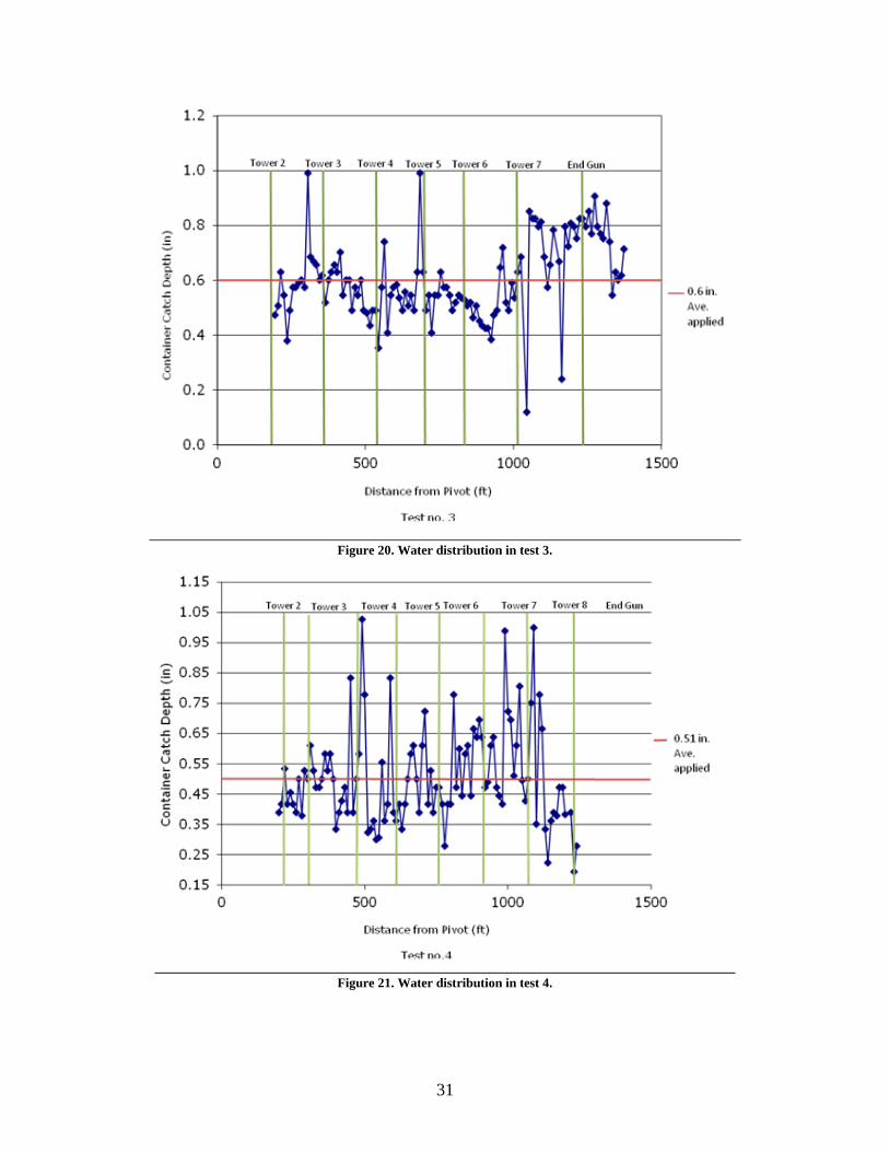
Figure 20. Water distribution in test 3. ............................................................................. 31

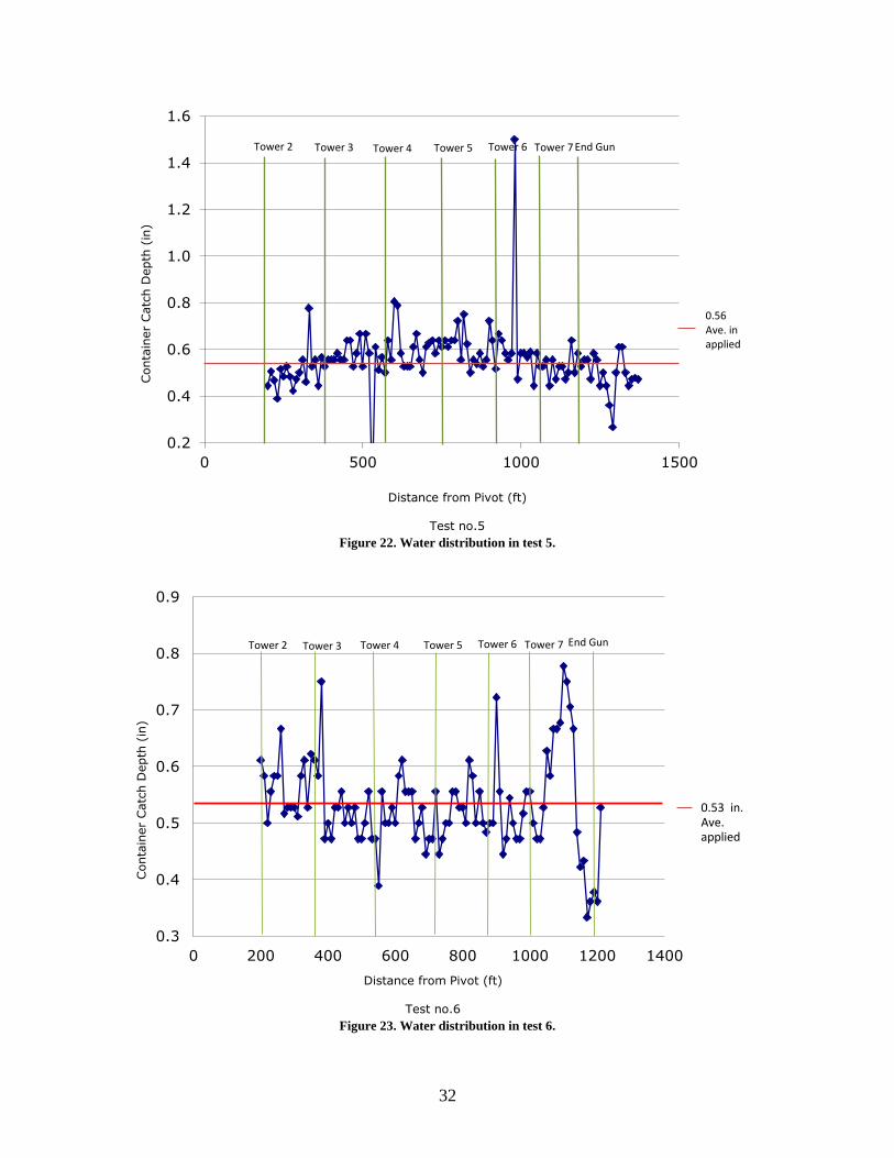
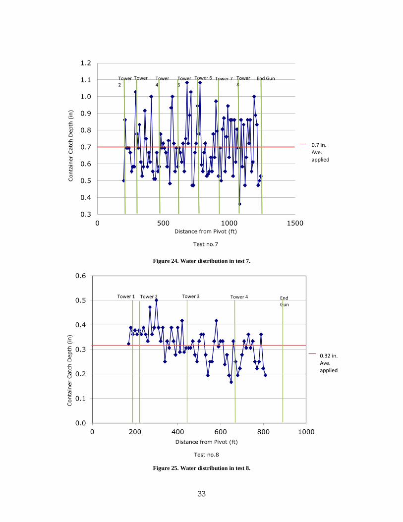
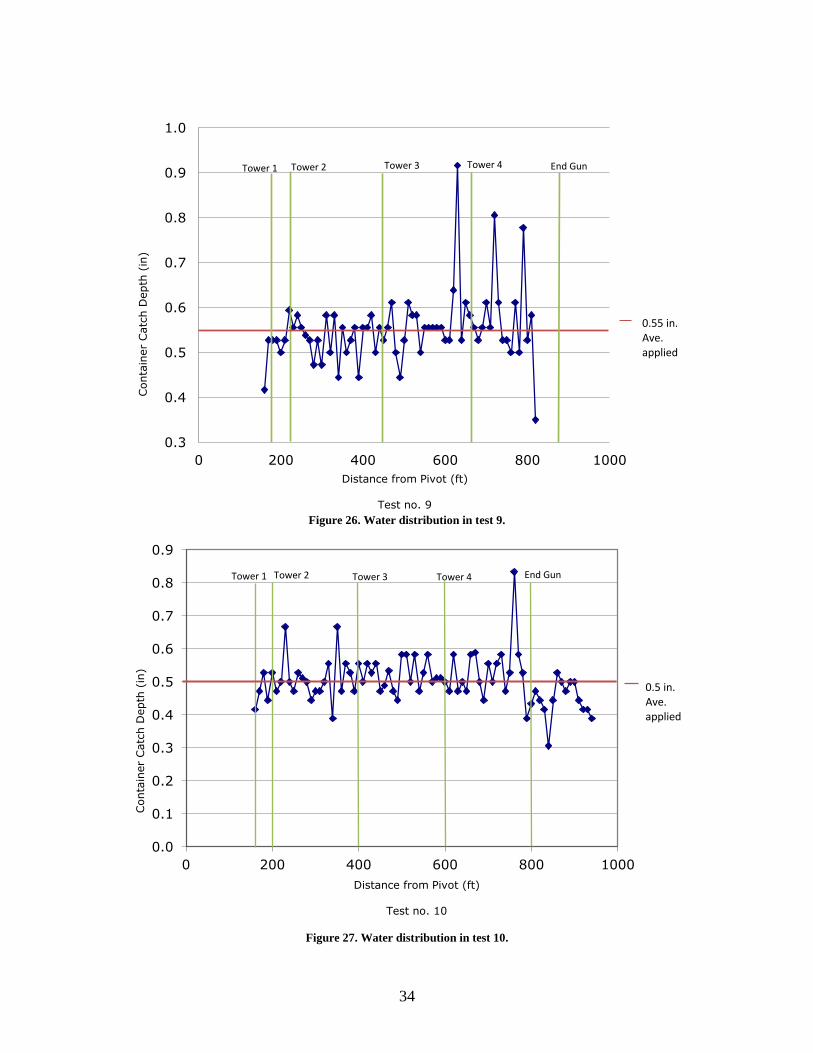
Figure 21. Water distribution in test 4. ............................................................................. 31 Figure 22. Water distribution in test 5. ............................................................................. 32 Figure 23. Water distribution in test 6. ............................................................................. 32 Figure 24. Water distribution in test 7. ............................................................................. 33 Figure 25. Water distribution in test 8. ............................................................................. 33 Figure 26. Water distribution in test 9. ............................................................................. 34 Figure 27. Water distribution in test 10. ........................................................................... 34

4

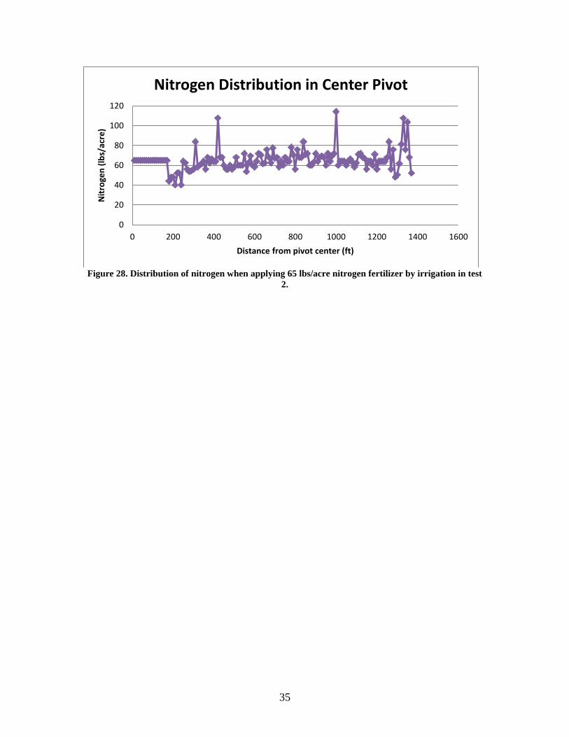
Figure 28. Distribution of nitrogen when applying 65 lbs/acre nitrogen fertilizer by

irrigation in test 2. ............................................................................................................. 35 Figure 29. Soil texture identification triangle. .................................................................. 36

5

Introduction Center pivot irrigation systems are invented over 60 years ago to reduce labor

requirements, enhance agricultural production, and optimize water use. According to

USDA Farm and Ranch Irrigation Survey in 2008 (2), center pivot irrigation are used on

the majority of sprinkler-irrigated land in United States and represent 83% from all types

of sprinkler systems.

A center pivot consists of a lateral circulating around a fixed pivot point. The lateral is

supported above the field by a series of A-frame towers, each tower having two driven

wheels at the base.

Water is discharged under pressure from sprinklers or sprayers mounted on the laterals as

it sweeps across the field or suspended by flexible hose over the crops. The lateral line is

rotated slowly around a pivot point at the center of the field by electric motors at each

tower.

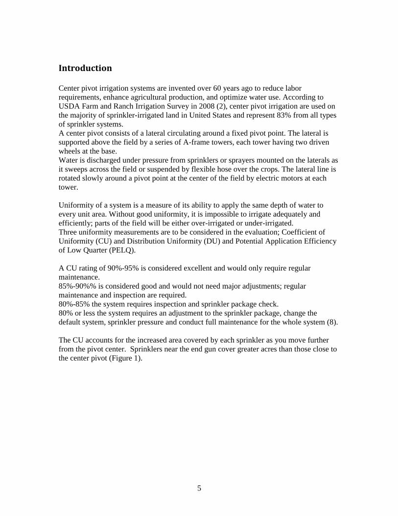
Uniformity of a system is a measure of its ability to apply the same depth of water to

every unit area. Without good uniformity, it is impossible to irrigate adequately and

efficiently; parts of the field will be either over-irrigated or under-irrigated.

Three uniformity measurements are to be considered in the evaluation; Coefficient of

Uniformity (CU) and Distribution Uniformity (DU) and Potential Application Efficiency

of Low Quarter (PELQ).

A CU rating of 90%-95% is considered excellent and would only require regular

maintenance.

85%-90%% is considered good and would not need major adjustments; regular

maintenance and inspection are required.

80%-85% the system requires inspection and sprinkler package check.

80% or less the system requires an adjustment to the sprinkler package, change the

default system, sprinkler pressure and conduct full maintenance for the whole system (8).

The CU accounts for the increased area covered by each sprinkler as you move further

from the pivot center. Sprinklers near the end gun cover greater acres than those close to

the center pivot (Figure 1).

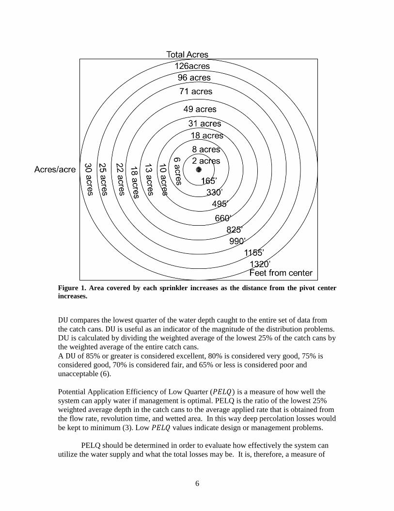
6

Figure 1. Area covered by each sprinkler increases as the distance from the pivot center

increases.

compares the lowest quarter of the water depth caught to the entire set of data from

the catch cans. is useful as an indicator of the magnitude of the distribution problems.

DU is calculated by dividing the weighted average of the lowest 25% of the catch cans by

the weighted average of the entire catch cans.

A of 85% or greater is considered excellent, 80% is considered very good, 75% is

considered good, 70% is considered fair, and 65% or less is considered poor and

unacceptable (6).

Potential Application Efficiency of Low Quarter ( is a measure of how well the

system can apply water if management is optimal. PELQ is the ratio of the lowest 25%

weighted average depth in the catch cans to the average applied rate that is obtained from

the flow rate, revolution time, and wetted area. In this way deep percolation losses would

be kept to minimum (3). Low values indicate design or management problems.

PELQ should be determined in order to evaluate how effectively the system can

utilize the water supply and what the total losses may be. It is, therefore, a measure of

7

the best management practice and should bet thought of as the full potential of the

system.

Background and Recent Research

6.4% of agriculture in Michigan irrigates crops at one point throughout the growing

season according to the United States Department of Agriculture (USDA). Michigan

uses 81 billion gallons of water to irrigate field crops annually extracting it from

groundwater, surface water, and the Great Lakes combined (5). When using this much

water for irrigation in Michigan alone, and fresh water being a scarce resource in many

parts of the world, it is important to make irrigation systems as efficient as possible with

minimal losses involved.

Most irrigation equipment in Michigan has not been evaluated for system uniformity.

Systems can be new to over 25 years old or older. Older systems can have greater water

losses due to leaking joints, clogged sprinklers, rusted equipment, etc.

Knowledge of changes in the magnitude water applied over time is important to

determine the causes of deficiencies in application rates and uniformities. Non-uniform

water application leads to over or under irrigation in various parts of the field which can

result in wasted water and energy and the potential for nitrogen leaching. This

information is needed to efficiently and effectively manage irrigation.

Water is pumped from a well or nearby water source to the center of the pivot where it is

distributed along the lateral pipe. Water is applied through sprinklers on that can be

attached directly to the pipe or hang down on hoses called drop nozzles.

Many recent developments have focused on improved control of center pivot irrigation

systems and incorporation of GPS equipment to all application of varying depths of water

to different field sectors. Manufactures and researchers are also working to integrate soil

water and plant sensors into center –pivot control. This enhanced monitoring promises to

optimize water use but at a high price for the time being (2).

For more improvement to the system performance, center pivot may be provided with

self-powered infrared thermometers and a GPS receiver on a center pivot lateral,

additional with remote spatial and temporal crop monitoring is accomplished by locating

sensors within a field. The resulting is automatic irrigation scheduling without using any

traditional tools for soil water content sensing and without using the traditional irrigation

scheduling (2).

8

Objectives

The objectives for this study are:

1) Evaluate the Uniformity of Coefficient, Distribution Uniformity and Potential

Application Efficiency through the season of crop growing and under field

conditions providing necessary information for more effective water management.

2) Use the Fluxus F601ultra-sonic flow meter device for measuring the accurate

flow system, and compare the volume of water applied to the irrigation area by

the system with the volume of water caught by catch cups.

3) Compare between different types of the center pivot sprinkler systems.

4) Recommend improvements for the performance operation of the center pivot

systems.

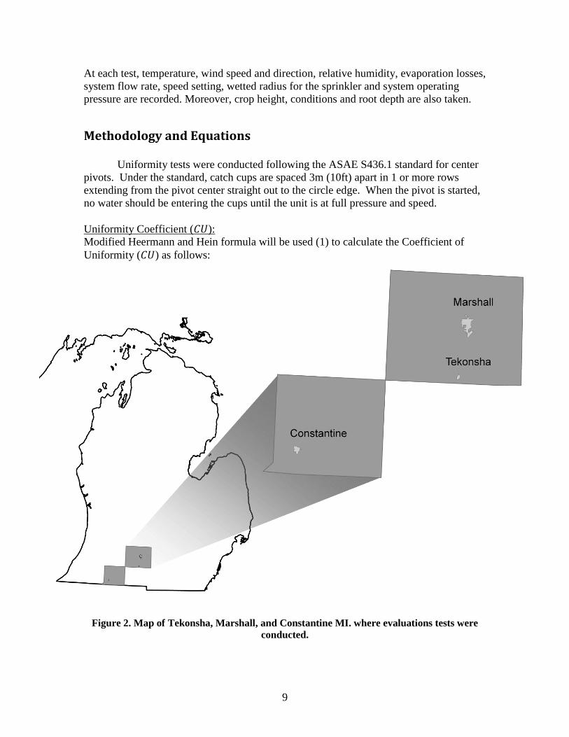
Study Area and Systems Description

Center pivot sprinkler irrigation systems are used in the Marshall, Tekonsha and

Constantine areas in Calhoun County and St. Joseph County of Michigan State (Figure

1), to irrigate corn, seed corn and soybeans. The evaluations took place during and end of

the 2011 irrigation season (June, July, August, September and October). Five farms were

selected using different crops and systems manufactures for the evaluation test. Ten

evaluation tests were done on these farms under varying weather conditions.

Center pivot systems in Tekonsha and Marshall consist of 7 and 8 towers plus end gun

tower respectively. Rotating sprays are used in Tekonsha field and fixed sprays in

Marshal. The field in Constantine consists of 4 tower plus an end gun with rotating sprays

suspended from the lateral.

Lengths of the towers and numbers of sprinklers are different from one system to the

other.

Sources of irrigation water are ground water, local rivers, and ponds.

Fields in Marshall and Constantine are flat; the field in Tekonsha has a gently rolling

topography.

The evaluation test method and procedure are performed based on the ASAE standard

S436.1 (1), and Merriam and Keller (6).

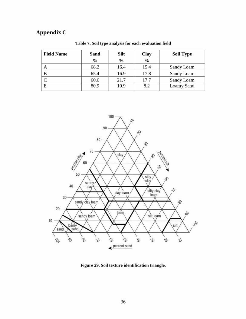
Soil samples were taken from each evaluation field before the irrigation system was

turned on. Soil type and moisture content was determined at MSU soil laboratories. All

fields’ soil is Sandy Loam except the field in Constantine town was Loamy Sand. Soil

analysis tests are shown in Table 6 (Appendix C).

9

At each test, temperature, wind speed and direction, relative humidity, evaporation losses,

system flow rate, speed setting, wetted radius for the sprinkler and system operating

pressure are recorded. Moreover, crop height, conditions and root depth are also taken.

Methodology and Equations Uniformity tests were conducted following the ASAE S436.1 standard for center

pivots. Under the standard, catch cups are spaced 3m (10ft) apart in 1 or more rows

extending from the pivot center straight out to the circle edge. When the pivot is started,

no water should be entering the cups until the unit is at full pressure and speed.

Uniformity Coefficient ( ):

Modified Heermann and Hein formula will be used (1) to calculate the Coefficient of

Uniformity ( ) as follows:

Figure 2. Map of Tekonsha, Marshall, and Constantine MI. where evaluations tests were

conducted.

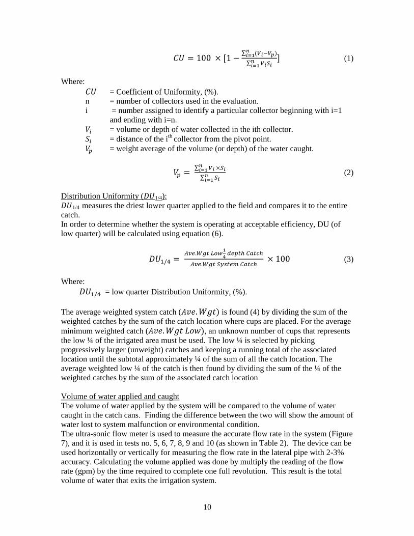
10

∑

∑

(1)

Where:

= Coefficient of Uniformity, (%).

n = number of collectors used in the evaluation.

i = number assigned to identify a particular collector beginning with i=1

and ending with i=n.

= volume or depth of water collected in the ith collector.

= distance of the ith

collector from the pivot point.

= weight average of the volume (or depth) of the water caught.

∑

∑

(2)

Distribution Uniformity ( 1/4):

1/4 measures the driest lower quarter applied to the field and compares it to the entire

catch.

In order to determine whether the system is operating at acceptable efficiency, DU (of

low quarter) will be calculated using equation (6).

(3)

Where:

= low quarter Distribution Uniformity, (%).

The average weighted system catch ( is found (4) by dividing the sum of the

weighted catches by the sum of the catch location where cups are placed. For the average

minimum weighted catch ( , an unknown number of cups that represents

the low ¼ of the irrigated area must be used. The low ¼ is selected by picking

progressively larger (unweight) catches and keeping a running total of the associated

location until the subtotal approximately ¼ of the sum of all the catch location. The

average weighted low ¼ of the catch is then found by dividing the sum of the ¼ of the

weighted catches by the sum of the associated catch location

Volume of water applied and caught

The volume of water applied by the system will be compared to the volume of water

caught in the catch cans. Finding the difference between the two will show the amount of

water lost to system malfunction or environmental condition.

The ultra-sonic flow meter is used to measure the accurate flow rate in the system (Figure

7), and it is used in tests no. 5, 6, 7, 8, 9 and 10 (as shown in Table 2). The device can be

used horizontally or vertically for measuring the flow rate in the lateral pipe with 2-3%

accuracy. Calculating the volume applied was done by multiply the reading of the flow

rate (gpm) by the time required to complete one full revolution. This result is the total

volume of water that exits the irrigation system.

11

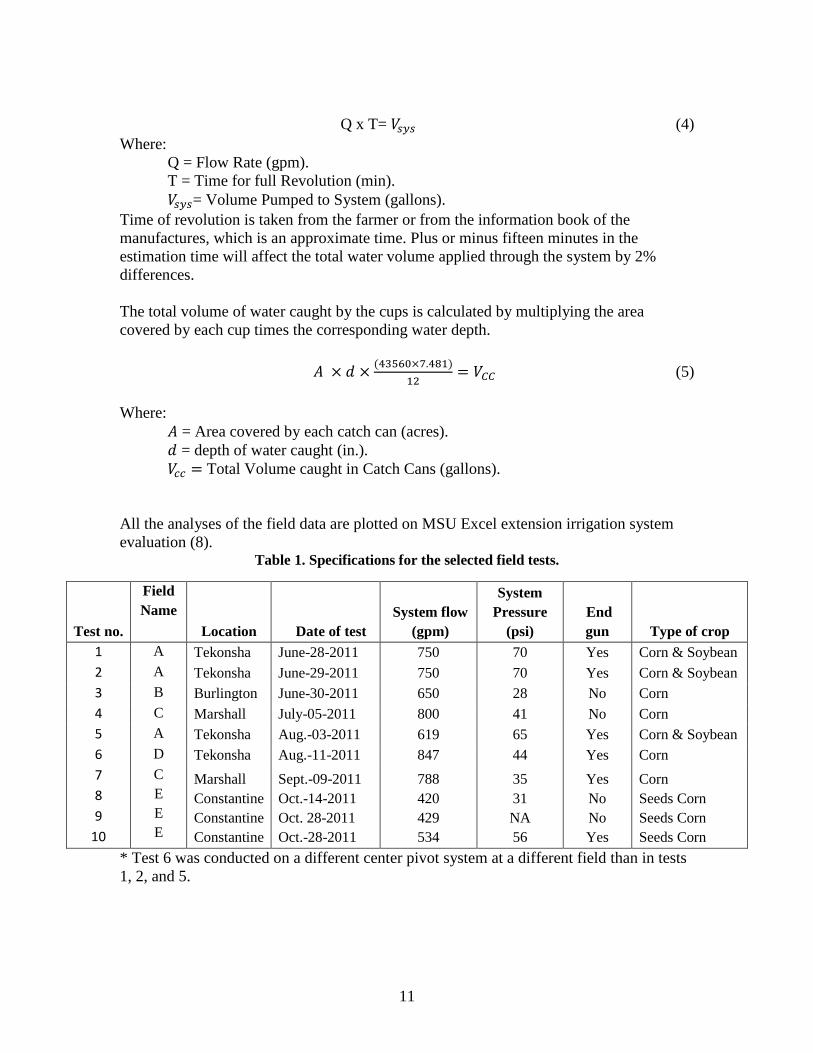
Q x T= (4)

Where:

Q = Flow Rate (gpm).

T = Time for full Revolution (min).

= Volume Pumped to System (gallons).

Time of revolution is taken from the farmer or from the information book of the

manufactures, which is an approximate time. Plus or minus fifteen minutes in the

estimation time will affect the total water volume applied through the system by 2%

differences.

The total volume of water caught by the cups is calculated by multiplying the area

covered by each cup times the corresponding water depth.

(5)

Where:

= Area covered by each catch can (acres).

= depth of water caught (in.).

Total Volume caught in Catch Cans (gallons).

All the analyses of the field data are plotted on MSU Excel extension irrigation system

evaluation (8). Table 1. Specifications for the selected field tests.

Test no.

Field

Name

Location Date of test

System flow

(gpm)

System

Pressure

(psi)

End

gun Type of crop

1 A Tekonsha June-28-2011 750 70 Yes Corn & Soybean

2 A Tekonsha June-29-2011 750 70 Yes Corn & Soybean

3 B Burlington June-30-2011 650 28 No Corn

4 C Marshall July-05-2011 800 41 No Corn

5 A Tekonsha Aug.-03-2011 619 65 Yes Corn & Soybean

6 D Tekonsha Aug.-11-2011 847 44 Yes Corn

7

8

9

10

C

E

E

E

Marshall

Constantine

Constantine

Constantine

Sept.-09-2011

Oct.-14-2011

Oct. 28-2011

Oct.-28-2011

788

420

429

534

35

31

NA

56

Yes

No

No

Yes

Corn

Seeds Corn

Seeds Corn

Seeds Corn

* Test 6 was conducted on a different center pivot system at a different field than in tests

1, 2, and 5.

12

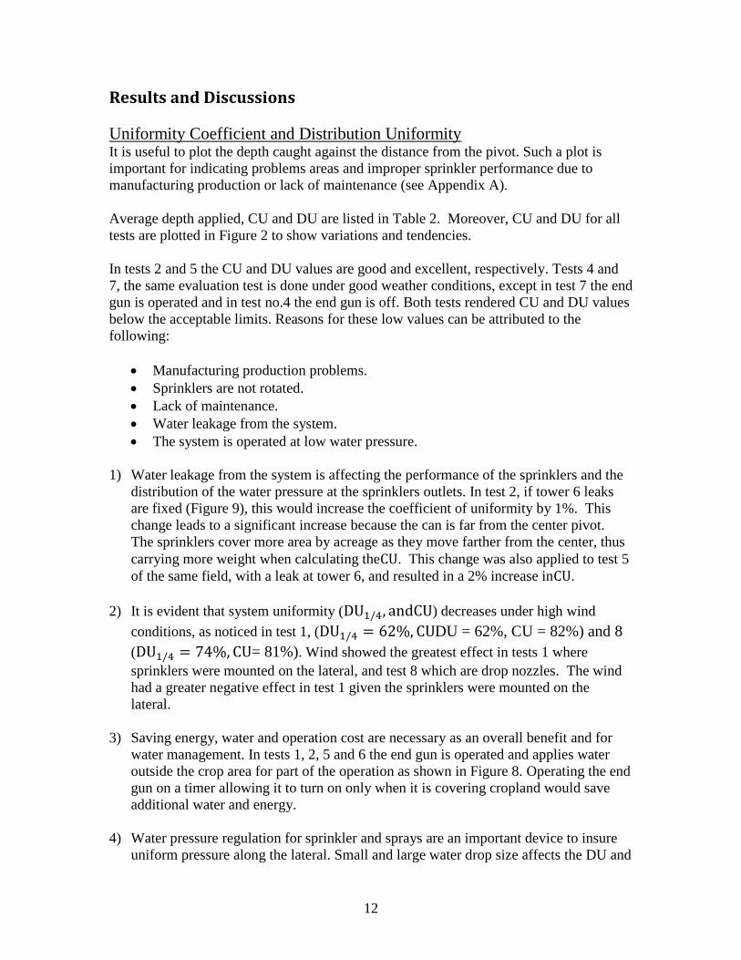
Results and Discussions

Uniformity Coefficient and Distribution Uniformity It is useful to plot the depth caught against the distance from the pivot. Such a plot is

important for indicating problems areas and improper sprinkler performance due to

manufacturing production or lack of maintenance (see Appendix A).

Average depth applied, CU and DU are listed in Table 2. Moreover, CU and DU for all

tests are plotted in Figure 2 to show variations and tendencies.

In tests 2 and 5 the CU and DU values are good and excellent, respectively. Tests 4 and

7, the same evaluation test is done under good weather conditions, except in test 7 the end

gun is operated and in test no.4 the end gun is off. Both tests rendered CU and DU values

below the acceptable limits. Reasons for these low values can be attributed to the

following:

Manufacturing production problems.

Sprinklers are not rotated.

Lack of maintenance.

Water leakage from the system.

The system is operated at low water pressure.

1) Water leakage from the system is affecting the performance of the sprinklers and the

distribution of the water pressure at the sprinklers outlets. In test 2, if tower 6 leaks

are fixed (Figure 9), this would increase the coefficient of uniformity by 1%. This

change leads to a significant increase because the can is far from the center pivot.

The sprinklers cover more area by acreage as they move farther from the center, thus

carrying more weight when calculating the . This change was also applied to test 5

of the same field, with a leak at tower 6, and resulted in a 2% increase in .

2) It is evident that system uniformity ( ) decreases under high wind

conditions, as noticed in test 1, ( DU = 62%, CU = 82%) and 8

( = 81%). Wind showed the greatest effect in tests 1 where

sprinklers were mounted on the lateral, and test 8 which are drop nozzles. The wind

had a greater negative effect in test 1 given the sprinklers were mounted on the

lateral.

3) Saving energy, water and operation cost are necessary as an overall benefit and for

water management. In tests 1, 2, 5 and 6 the end gun is operated and applies water

outside the crop area for part of the operation as shown in Figure 8. Operating the end

gun on a timer allowing it to turn on only when it is covering cropland would save

additional water and energy.

4) Water pressure regulation for sprinkler and sprays are an important device to insure

uniform pressure along the lateral. Small and large water drop size affects the DU and

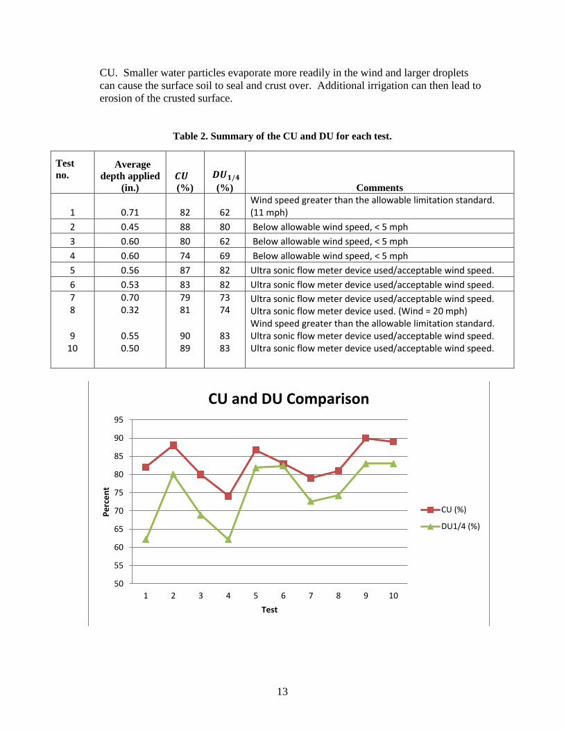
13

CU. Smaller water particles evaporate more readily in the wind and larger droplets

can cause the surface soil to seal and crust over. Additional irrigation can then lead to

erosion of the crusted surface.

Table 2. Summary of the CU and DU for each test.

Test

no.

Average

depth applied

(in.)

(%)

(%) Comments

1 0.71 82 62 Wind speed greater than the allowable limitation standard. (11 mph)

2 0.45 88 80 Below allowable wind speed, < 5 mph



5 0.56 87 82 Ultra sonic flow meter device used/acceptable wind speed.

6 0.53 83 82 Ultra sonic flow meter device used/acceptable wind speed. 7 8

9 10

0.70 0.32

0.55 0.50

79 81

90 89

73 74

83 83

Ultra sonic flow meter device used/acceptable wind speed. Ultra sonic flow meter device used. (Wind = 20 mph) Wind speed greater than the allowable limitation standard. Ultra sonic flow meter device used/acceptable wind speed. Ultra sonic flow meter device used/acceptable wind speed.

50

55

60

65

70

75

80

85

90

95

1 2 3 4 5 6 7 8 9 10

Pe

rce

nt

Test

CU and DU Comparison

CU (%)

DU1/4 (%)

14

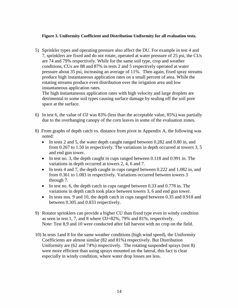
Figure 3. Uniformity Coefficient and Distribution Uniformity for all evaluation tests.

5) Sprinkler types and operating pressure also affect the DU. For example in test 4 and

7, sprinklers are fixed and do not rotate, operated at water pressure of 25 psi, the CUs

are 74 and 79% respectively. While for the same soil type, crop and weather

conditions, CUs are 88 and 87% in tests 2 and 5 respectively operated at water

pressure about 35 psi, increasing an average of 11%. Then again, fixed spray streams

produce high instantaneous application rates on a small percent of area. While the

rotating streams produce even distribution over the irrigation area and low

instantaneous application rates.

The high instantaneous application rates with high velocity and large droplets are

detrimental to some soil types causing surface damage by sealing off the soil pore

space at the surface.

6) In test 6, the value of was 83% (less than the acceptable value, 85%) was partially

due to the overhanging canopy of the corn leaves in some of the evaluation zones.

8) From graphs of depth catch vs. distance from pivot in Appendix A, the following was

noted:

In tests 2 and 5, the water depth caught ranged between 0.282 and 0.80 in, and

from 0.267 to 1.50 in respectively. The variations in depth occurred at towers 3, 5

and end gun tower.

In test no. 3, the depth caught in cups ranged between 0.118 and 0.991 in. The

variations in depth occurred at towers 2, 4, 6 and 7.

In tests 4 and 7, the depth caught in cups ranged between 0.222 and 1.082 in, and

from 0.361 to 1.083 in respectively. Variations occurred between towers 3

through 7.

In test no. 6, the depth catch in cups ranged between 0.33 and 0.778 in. The

variations in depth catch took place between towers 3, 6 and end gun tower.

In tests nos. 9 and 10, the depth catch in cups ranged between 0.35 and 0.918 and

between 0.305 and 0.833 respectively.

9) Rotator sprinklers can provide a higher CU than fixed type even in windy condition

as seen in test 1, 7, and 8 where =82%, 79% and 81%, respectively.

Note: Test 8,9 and 10 were conducted after fall harvest with no crop on the field.

10) In tests 1and 8 for the same weather conditions (high wind speed), the Uniformity

Coefficients are almost similar (82 and 81%) respectively. But Distribution

Uniformity are (62 and 74%) respectively. The rotating suspended sprays (test 8)

were more efficient than using sprays mounted on the lateral, this fact is clear

especially in windy condition, where water drop losses are less.

15

11) Systems with rotating drop nozzles had greater Uniformity Coefficient and

Distribution Uniformity than the rotating sprays mounted on the lateral by about 2%

as an average value. Likewise, the drop downs had better uniformity than the fixed

sprays mounted on the lateral by about 14% as an average value.

12) In tests 8, 9, and 10, water pressure from sprays in tower no. 1 are less than other

sprays. This is due to the pressure regulation device default.

13) and DU can be expressed in terms of coefficient of variation, if a normal

distribution is assumed for the distribution of water. Equation (6) gives the

statistically derived estimate for the uniformity when >70%. is approximately

related:

(6)

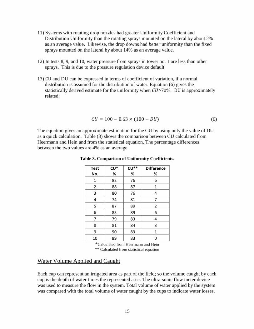
The equation gives an approximate estimation for the CU by using only the value of DU

as a quick calculation. Table (3) shows the comparison between CU calculated from

Heermann and Hein and from the statistical equation. The percentage differences

between the two values are 4% as an average.

Table 3. Comparison of Uniformity Coefficients.

Test No.

CU* %

CU** %

Difference %

1 82 76 6

2 88 87 1

3 80 76 4

4 74 81 7

5 87 89 2

6 83 89 6

7 79 83 4

8 81 84 3

9 90 83 1

10 89 83 0 *Calculated from Heermann and Hein

** Calculated from statistical equation

Water Volume Applied and Caught

Each cup can represent an irrigated area as part of the field; so the volume caught by each

cup is the depth of water times the represented area. The ultra-sonic flow meter device

was used to measure the flow in the system. Total volume of water applied by the system

was compared with the total volume of water caught by the cups to indicate water losses.

16

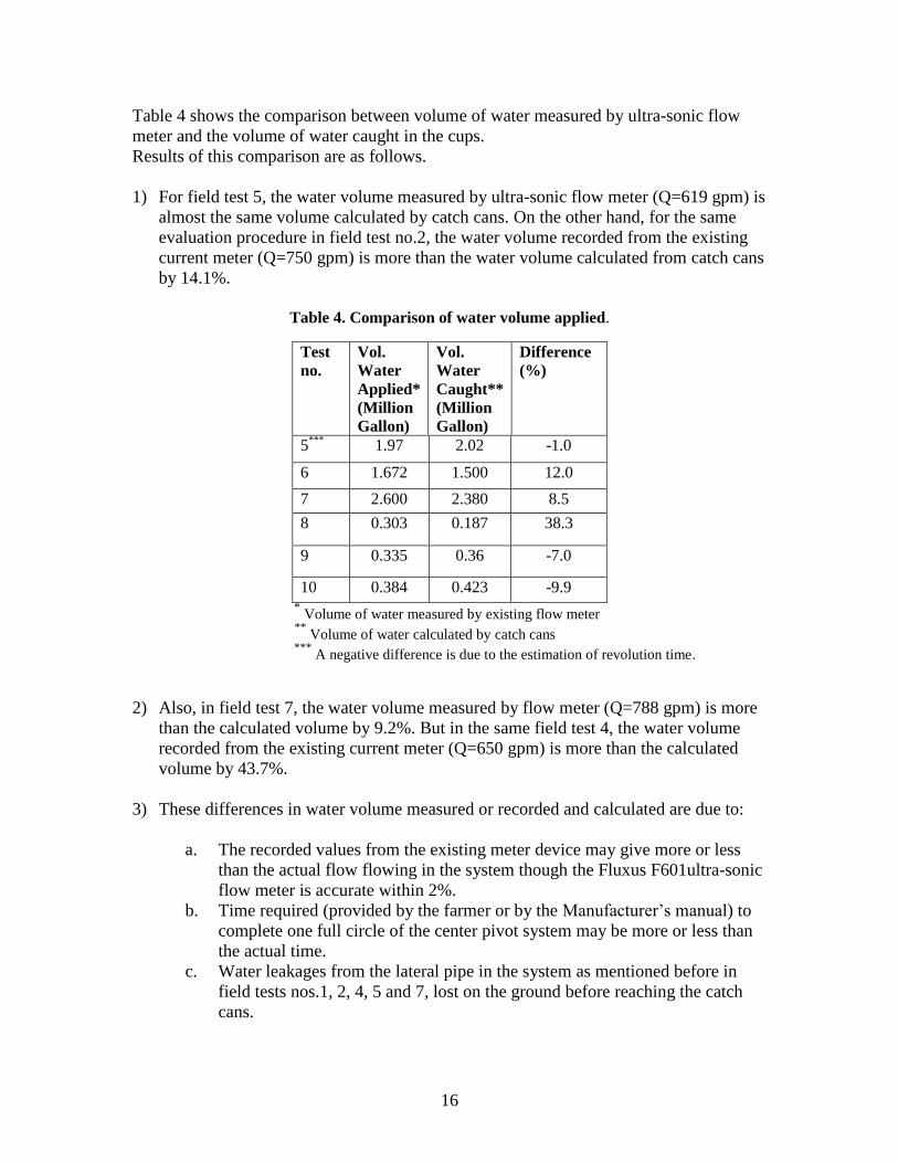
Table 4 shows the comparison between volume of water measured by ultra-sonic flow

meter and the volume of water caught in the cups.

Results of this comparison are as follows.

1) For field test 5, the water volume measured by ultra-sonic flow meter (Q=619 gpm) is

almost the same volume calculated by catch cans. On the other hand, for the same

evaluation procedure in field test no.2, the water volume recorded from the existing

current meter (Q=750 gpm) is more than the water volume calculated from catch cans

by 14.1%.

Table 4. Comparison of water volume applied.

Test

no.

Vol.

Water

Applied*

(Million

Gallon)

Vol.

Water

Caught**

(Million

Gallon)

Difference (%)

5***

1.97 2.02 -1.0

6

1.672 1.500 12.0

7 2.600 2.380 8.5

8

0.303 0.187 38.3

9 0.335 0.36 -7.0

10 0.384 0.423 -9.9 *

Volume of water measured by existing flow meter **

Volume of water calculated by catch cans

***

A negative difference is due to the estimation of revolution time.

2) Also, in field test 7, the water volume measured by flow meter (Q=788 gpm) is more

than the calculated volume by 9.2%. But in the same field test 4, the water volume

recorded from the existing current meter (Q=650 gpm) is more than the calculated

volume by 43.7%.

3) These differences in water volume measured or recorded and calculated are due to:

a. The recorded values from the existing meter device may give more or less

than the actual flow flowing in the system though the Fluxus F601ultra-sonic

flow meter is accurate within 2%.

b. Time required (provided by the farmer or by the Manufacturer’s manual) to

complete one full circle of the center pivot system may be more or less than

the actual time.

c. Water leakages from the lateral pipe in the system as mentioned before in

field tests nos.1, 2, 4, 5 and 7, lost on the ground before reaching the catch

cans.

17

d. The canopy of the crop plant, especially corn, may also affect the volume of

water caught by the cups in the evaluation test if the cups are too close to the

crop line (test no.6).

4) The volume of water applied to the irrigation area can also be found from multiplying

the average depth applied by the irrigated area. The difference between the calculated

volumes from the average depth and the volume calculated from each cup caught by

is about 2.7%.

5) The big difference between water volumes applied and volume caught by cups in test

8 comparing with tests nos. 9 and 10 is due to the high wind speed.

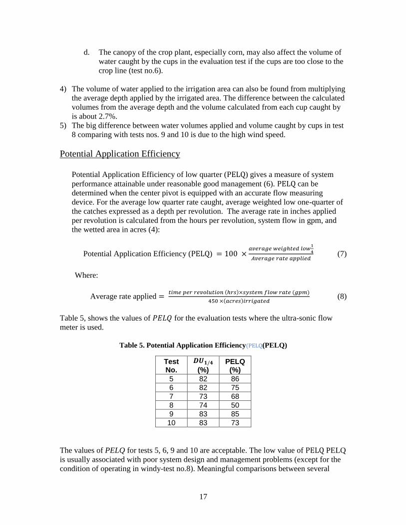
Potential Application Efficiency

Potential Application Efficiency of low quarter ( ) gives a measure of system

performance attainable under reasonable good management (6). can be

determined when the center pivot is equipped with an accurate flow measuring

device. For the average low quarter rate caught, average weighted low one-quarter of

the catches expressed as a depth per revolution. The average rate in inches applied

per revolution is calculated from the hours per revolution, system flow in gpm, and

the wetted area in acres (4):

Potential Application Efficiency ( )

(7)

Where:

Average rate applied

(8)

Table 5, shows the values of for the evaluation tests where the ultra-sonic flow

meter is used.

Table 5. Potential Application Efficiency (PELQ)

Test No.

(%) PELQ

(%)

5 82 86

6 82 75

7 73 68

8 74 50

9 83 85

10 83 73

The values of PELQ for tests 5, 6, 9 and 10 are acceptable. The low value of PELQ

is usually associated with poor system design and management problems (except for the

condition of operating in windy-test no.8). Meaningful comparisons between several

18

systems modifications or methods can be made by comparing values of PELQ. For

a proper system operation, PELQ should be similar to the value of DU.

Fertigation based on Uniformity

Liquid urea-ammonium nitrate (UAN) is the most common source of nitrogen

injected into irrigation water. It maintains a constant concentration without agitation, is

easy to transport and store. This practice of application of nitrogen is called nitrogen

fertigation.

Applying a portion of a crop’s nitrogen (N) requirement with irrigation water is a

recognized best management practice to reduce nitrate leaching losses for some crops

grown on coarse textured soils. For example, if the application rate of the irrigation

system is exceeding the soil intake rate, this will not provide adequate N distribution, and

some N will either leach into the ground in the areas where the water ponds or move into

surface water via runoff.

The potential for nitrate leaching loss from irrigated sandy soil is greater than for

finer texture, however, careful management of water and nitrogen can help limit loss.

Apply nitrogen with irrigation water only with systems that can provide a uniform water

application over entire field and at an application rate that does not exceed the infiltration

rate of the soil. Distribution of N through an irrigation system is no better than the same

system’s distribution of water. Center pivot irrigation systems can provide a very

uniform distribution of water and N if the sprinkler package is properly selected and

maintained. (10)

Calculations

Nitrogen applications in this study were calculated on a seasonal basis with

assuming rates of 65 and 200 lbs per acre. Using 200 lbs/ac was intended to show the

total amount of nitrogen applied to a field by fertigation only. This was then multiplied

by the acres covered by each sprinkler to give a total amount of nitrogen applied per

catch can over the season.

100% Uniformity TN = R x A (9)

Where,

TN = Total N (lbs) applied under perfect uniformity

A = Area covered per catch can (acre)

R = Application rate over a season (lbs/acre)

Actual Applied Nitrogen

AN = D x TN (10)

Where,

AN = Actual N (lbs)

D = Percent applied of average

The actual nitrogen applied was based on the amount of water that each catch can

received as compared to the average depth caught. For example, if a catch can received

0.4 in. water and the average was 0.45 in. the percent applied would be 89%. This value

19

was then multiplied by the pounds of N that would have been applied if the system

operated at 100% uniformity.

In order to rate the distribution uniformity of nitrogen, the average deviation was

calculated. At every catch can, the depth of water was translated to an applied rate of

nitrogen in lbs/acre. This was then compared to the average application rate (65 or 200

lbs/ac) and then divided by the total number of catch cans giving the deviation of the the

whole data set from the average intended application. Results follow.

Results and Analysis

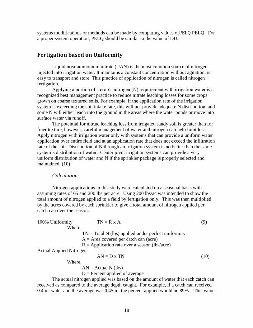
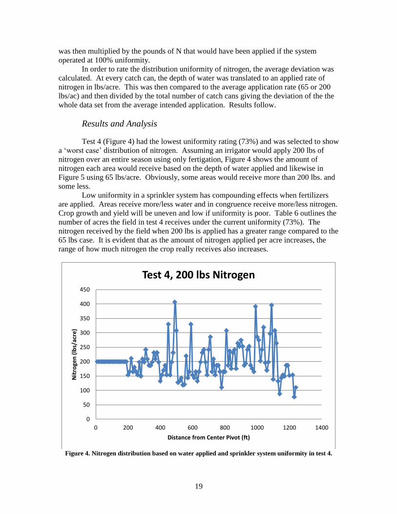
Test 4 (Figure 4) had the lowest uniformity rating (73%) and was selected to show

a ‘worst case’ distribution of nitrogen. Assuming an irrigator would apply 200 lbs of

nitrogen over an entire season using only fertigation, Figure 4 shows the amount of

nitrogen each area would receive based on the depth of water applied and likewise in

Figure 5 using 65 lbs/acre. Obviously, some areas would receive more than 200 lbs. and

some less.

Low uniformity in a sprinkler system has compounding effects when fertilizers

are applied. Areas receive more/less water and in congruence receive more/less nitrogen.

Crop growth and yield will be uneven and low if uniformity is poor. Table 6 outlines the

number of acres the field in test 4 receives under the current uniformity (73%). The

nitrogen received by the field when 200 lbs is applied has a greater range compared to the

65 lbs case. It is evident that as the amount of nitrogen applied per acre increases, the

range of how much nitrogen the crop really receives also increases.

Figure 4. Nitrogen distribution based on water applied and sprinkler system uniformity in test 4.

0

50

100

150

200

250

300

350

400

450

0 200 400 600 800 1000 1200 1400

Nit

roge

n (

lbs/

acre

)

Distance from Center Pivot (ft)

Test 4, 200 lbs Nitrogen

20

Figure 5. Nitrogen distribution in test 4 assuming 65 lbs/acre applied over the season by fertigation in

test 4.

Figure 6. Graph based on 200 lbs nitrogen application over a season via fertigation in test 4.

0

20

40

60

80

100

120

140

0 200 400 600 800 1000 1200 1400

Nit

roge

n (

lbs/

acre

)

Distance from Pivot Center (ft)


0

50

100

150

200

250

0 200 400 600 800 1000 1200 1400

Nit

roge

n A

pp

lied

(lb

s)


Actual Nitrogen Applied compared to 100% Uniformity

73% Uniformity100% Uniformity

21

Table 6. Number of acres that receive different amounts of Nitrogen in Test 4.

65 lbs 200 lbs

Nitrogen (lbs)

Number of

Acres Number of Acres

0-50 22

51-100 78 3

101-150 10 17

151-200 46

201-250 19

251-300 14

300+ 10

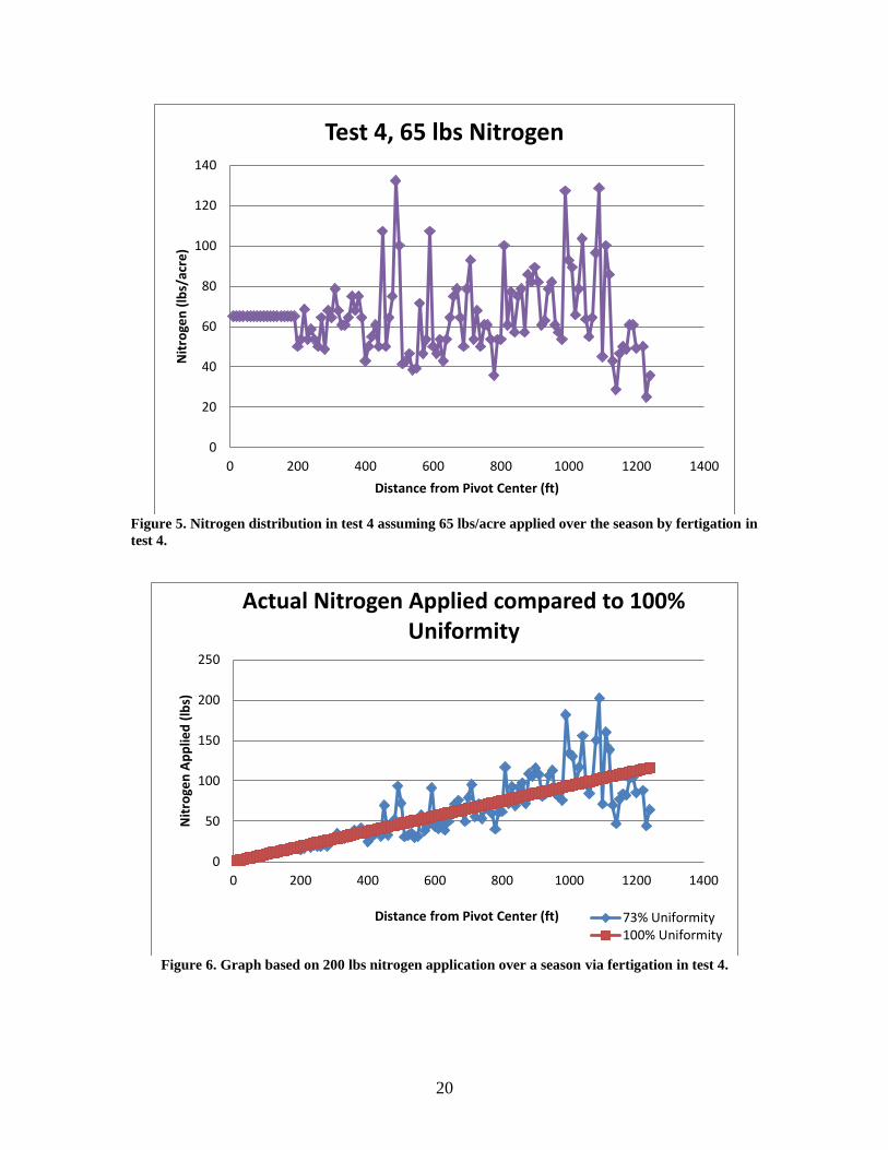
Figure 6 shows how the center pivot applies nitrogen (blue) based on water collected

from the cans. The red line indicates the amount of water applied if uniformity were at

100%.

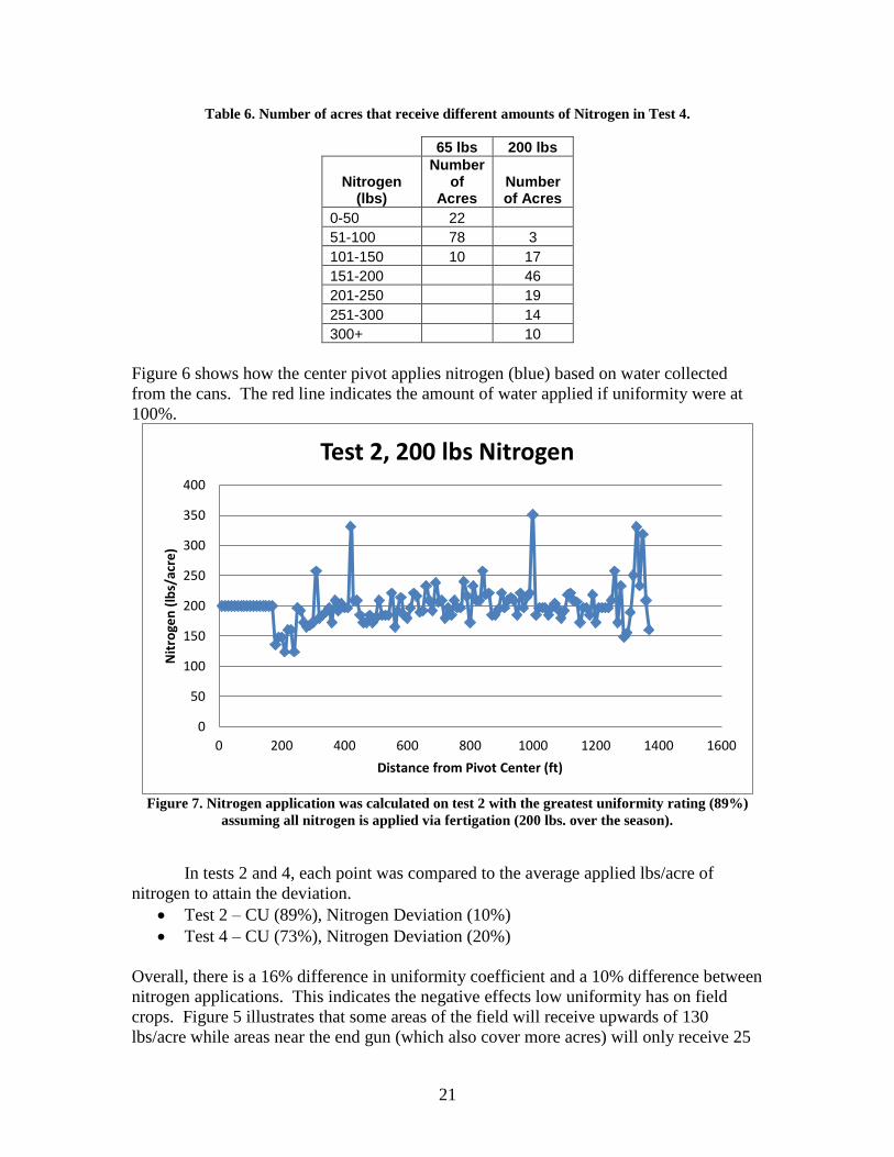
Figure 7. Nitrogen application was calculated on test 2 with the greatest uniformity rating (89%)

assuming all nitrogen is applied via fertigation (200 lbs. over the season).

In tests 2 and 4, each point was compared to the average applied lbs/acre of

nitrogen to attain the deviation.

Test 2 – CU (89%), Nitrogen Deviation (10%)

Test 4 – CU (73%), Nitrogen Deviation (20%)

Overall, there is a 16% difference in uniformity coefficient and a 10% difference between

nitrogen applications. This indicates the negative effects low uniformity has on field

crops. Figure 5 illustrates that some areas of the field will receive upwards of 130

lbs/acre while areas near the end gun (which also cover more acres) will only receive 25

0

50

100

150

200

250

300

350

400

0 200 400 600 800 1000 1200 1400 1600

Nit

roge

n (

lbs/

acre

)



22

lbs/acre. Add in a sloping topography and actual nitrogen distribution will decrease

significantly. Thus, it is crucial to regularly maintain a system and perform a type of

uniformity test or check to assure appropriate applications.

Similar to the water distribution graphs, there are certain areas where leaks

(Figure 7 at 420 and 1,000 ft) or irregular watering patterns occur. The higher

application rate in these sections could leach into the ground water and be lost to the plant

or collect in runoff. Runoff, which would take nitrogen away from the higher elevations,

would then pond and could percolate out past the plant roots making it unavailable.

Uniformity therefore has the potential to cost the farmer several times over when

fertigation is used in a system with poor uniformity.

Recommendations

Distribution Evaluations 1) Evaluation test should always be done in open area and catch cans should be far from

the canopy of the crop as shown in Figures 4 and 6.

2) Following ASAE S436.1standard it is suggested to run systems when winds are low,

preferably less than 5 mph and no greater than 11 mph.

3) Regular system maintenance is necessary including repair, adjustment or modification

to keep the system operated efficiently. If CUs are periodically measured (at least

annually) system repairs and adjustments can be scheduled when coefficients fall

below the desired values. This will save operation costs and conserve water.

4) Water pressure should be tested at the sprinkler outlet to ensure that each sprinkler

operates at the design pressure especially sprinkler(s) which give low or high volume

caught in catch cups, which affects the overall DU and CU.

5) Low uniformities in the center pivot system have compounding negative effects when

nitrogen is applied. Therefore, any major leaks and poor end gun performance need

to be fixed or adjusted to insure the highest uniformity possible.

System Improvement for a Uniform Distribution 6) Location of the pivot according to the field topography and time of operating end gun

should be considered.

7) The depth applied, timer setting and time of revolution should be set according to the

manufacturer information book, otherwise consultation from the manufacturer is

necessary.

8) Regular measuring system flow rate by accurate and modern flow meter is advised.

As a water management tool this helps reduce water costs, prevent over irrigation and

reduces leaching of chemicals and fertilizers into the ground.

9) Using available new technology can improve system performance.

10) Using rotating spray sprinklers is advised. Rotating spray types provides the widest

throw distance, is closest to matching infiltration rates of the soil and reduces water

surface runoff.

11) Drop down nozzles proved to distribute water evenly. This type of sprays would be

recommended where the nozzles do not enter the crop canopy because water

distribution is severely decreased once this occurs.

23

12) Operating of the pressure regulation for all sprays should be checked and replaced

when needed.

Acknowledgements

The authors want to thank Lyndon Kelley for his generous contribution.

This work is supported by Biosystems and Agricultural Engineering Department.

The writers thank Mark Sackrider, Ed Groholske , Ryan Groholske and Sally and

Dale Stuby for their coorporation performing evaluation tests in their field.

The writer thanks the staff in the research shop /Department of Biosystems and

Agricultural Engineering for their help with supporting the team work with tools.

Finally the writer thanks Daniel Morgan for his support doing fields tests and Sean

Woznicki for preparing the maps.

24

References

1- ANSI/ASAE S436.1, “Test Procedure for Determining the Uniformity of Water

Distribution of Center Pivot and Lateral Move Irrigation Machines Equipped with

Spray or Sprinkler Nozzles”, Jun1996 (R2007).

2- ASABE, Resouce, Engineering and Technology for a Sustainable World, Vol.18,

No. 5, September/October, 2011.

3- GW Asough and GA Kiker “The Effect of Irrigation Uniformmity on Irrigation

water Requirements” Water SA Vol. 28, No.2, April 2002.

4- Jack Keller and Bleisner RD “Sprinkler and Trickle Irrigation”, Van Nostrand

Reinhold, New York, 1990.

5- MAD Estimated Water Withdrawals for Irrigated Crops

in Michigan, by Crop Type, 2006.

6- Merriam, John L., and Jack Keller, “Irrigation System Evaluation and

Improvement” Utah State University, Logan , Utah, 1973.

7- Michael D. Dukes and Calvin Perry “Uniformity testing of variable-rate cenetr

pivot irrigation control systems” Precision Agric. Vol.7, pp205-218, 2006.

8- MSU Excell spreadsheet for the evaluation test, prepare by London Kelley.

9- Nelson irrigation Corporation “ water application solutions for Ccenter pivot

irrigation” 2004.

10- 10- Jerry Wright and et al “Nitrogen Application with irrigation water-

Chemigation”, University of Minnesota/Extension, clean water series, 2002.

25

Appendix A

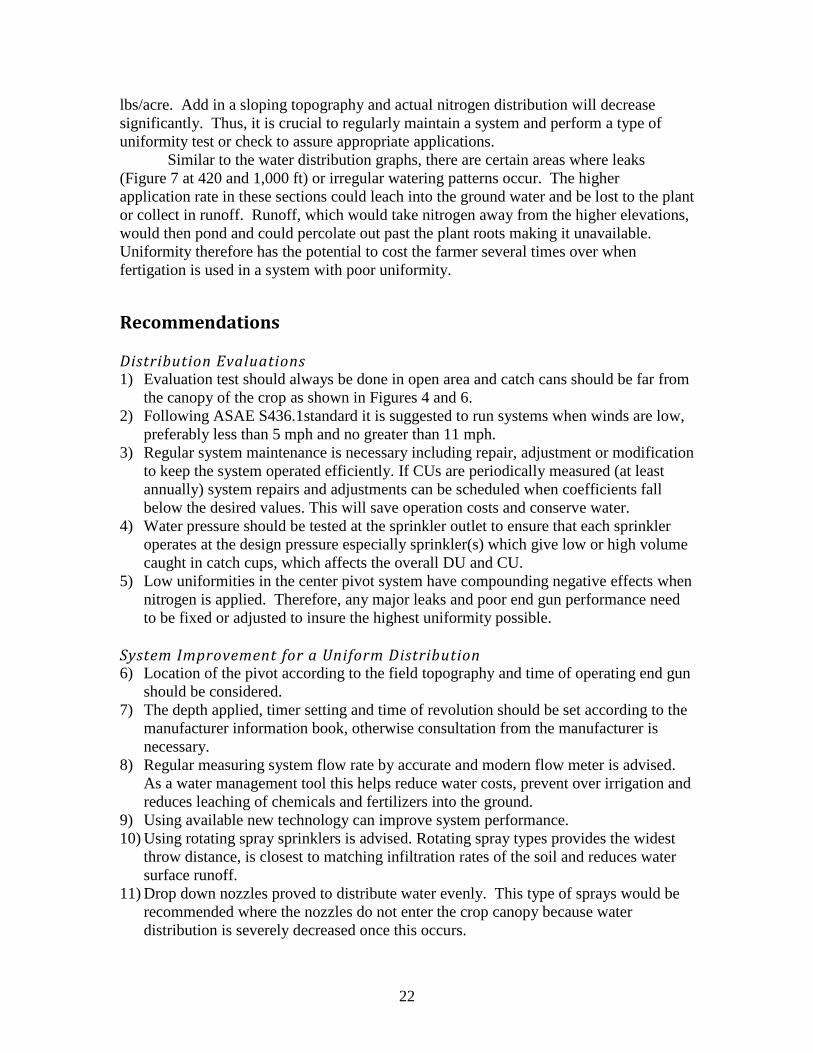
Figure 8. Rotating Sprays mounted on the lateral of the center pivot.

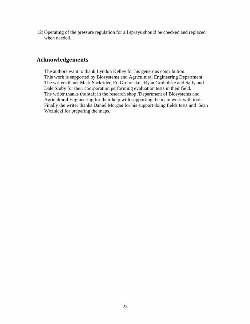
Figure 9. Catch cups lined up along the edge of the corn crop.

26

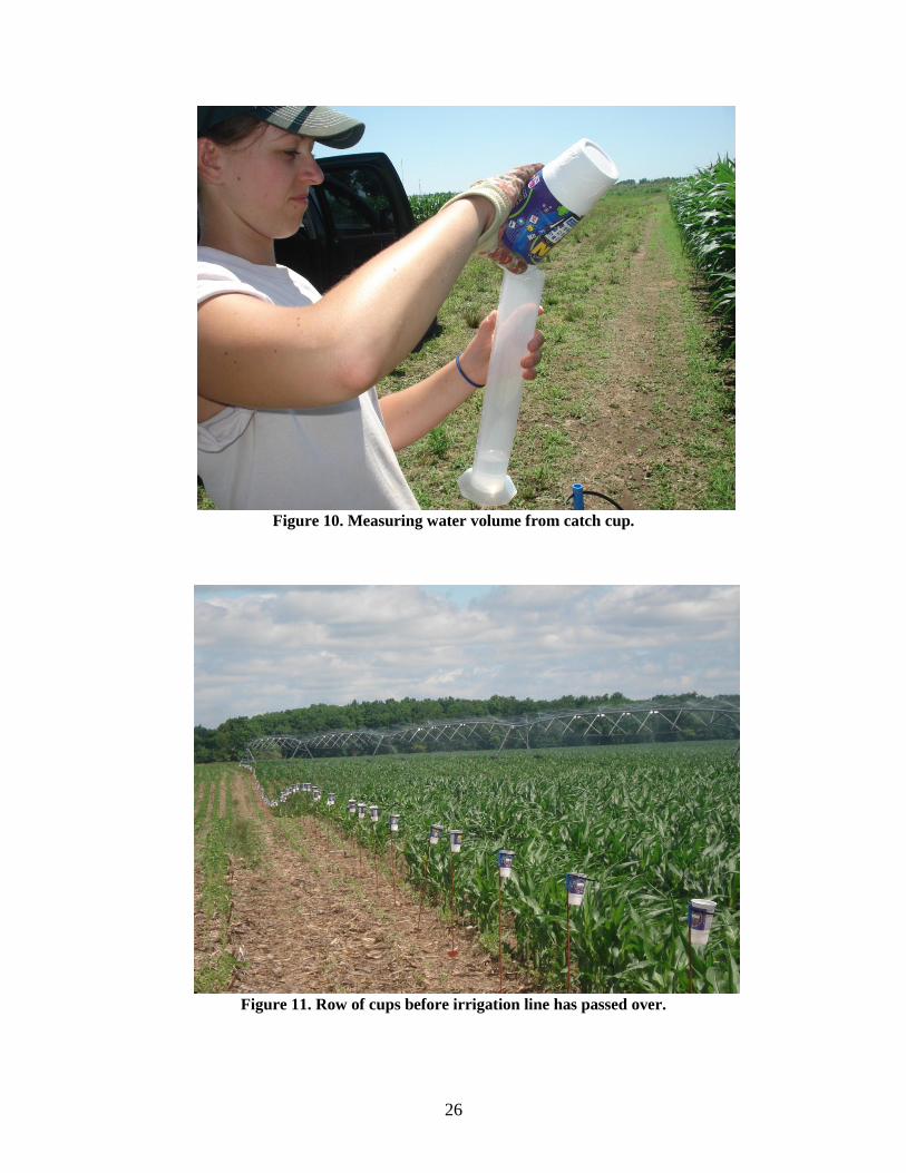
Figure 10. Measuring water volume from catch cup.

Figure 11. Row of cups before irrigation line has passed over.

27

Figure 12. Using the Ultra-sonic flow meter to measure flow rate through the

system.

Figure 13. Center pivot with end gun on.

28

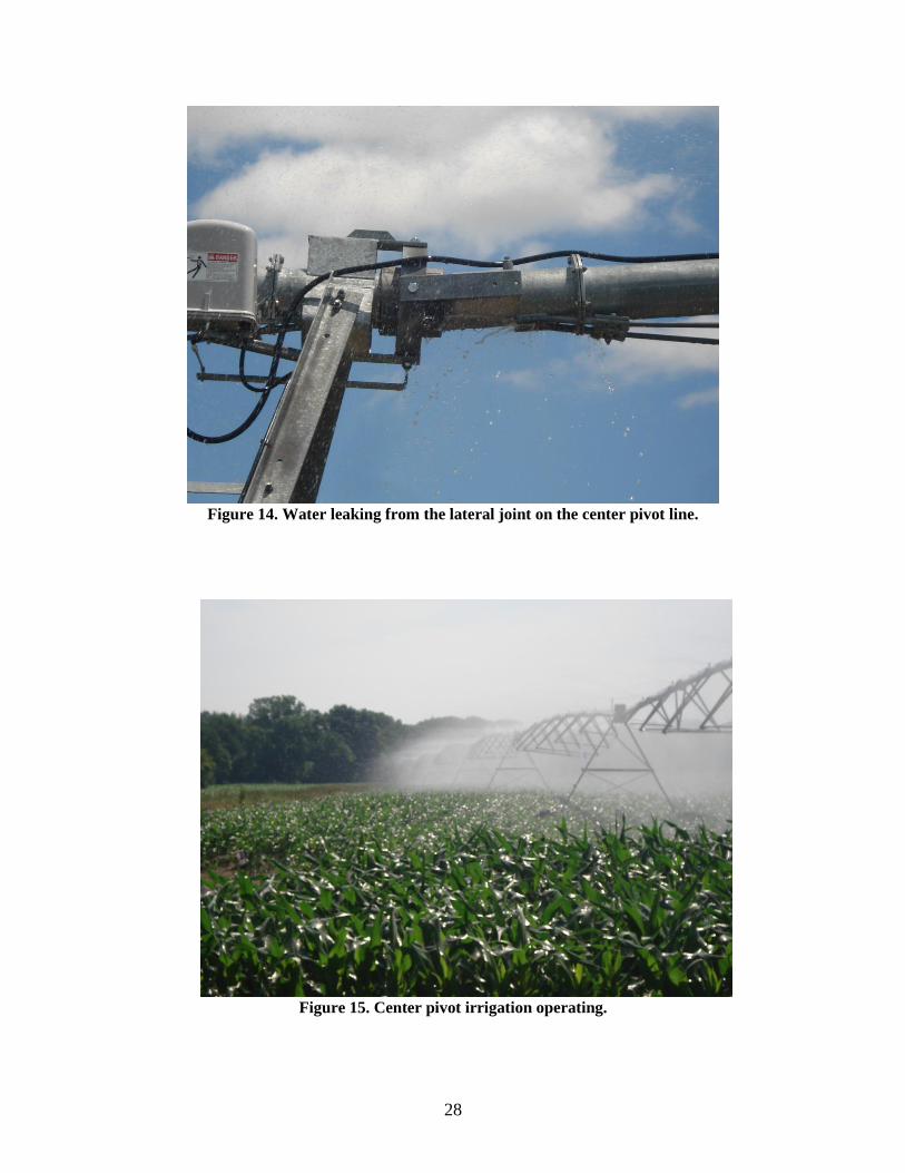
Figure 14. Water leaking from the lateral joint on the center pivot line.

Figure 15. Center pivot irrigation operating.

29

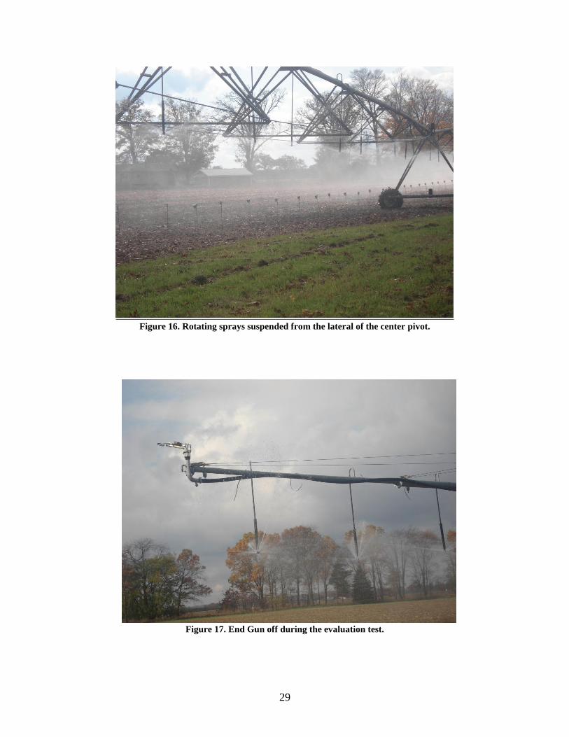
Figure 16. Rotating sprays suspended from the lateral of the center pivot.

Figure 17. End Gun off during the evaluation test.

30

Appendix B

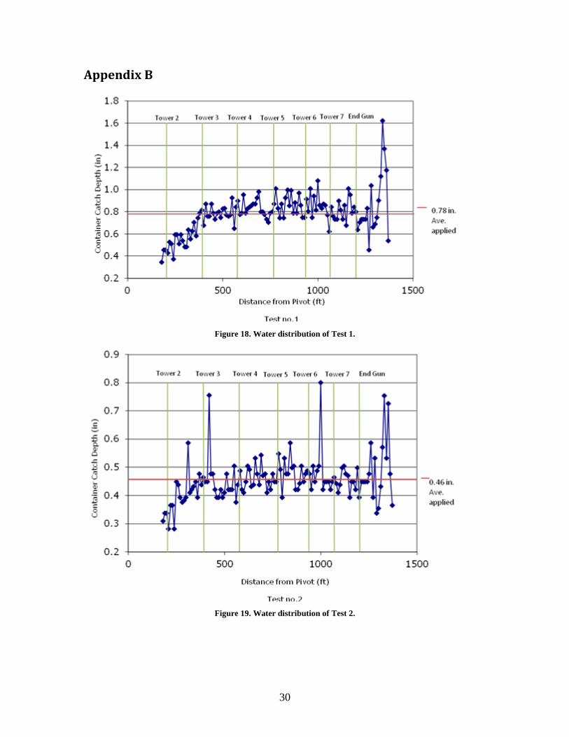
Figure 18. Water distribution of Test 1.

Figure 19. Water distribution of Test 2.

31

Figure 20. Water distribution in test 3.


32



0.2

0.4

0.6

0.8

1.0

1.2

1.4

1.6

0 500 1000 1500

Conta

iner

Catc

h D

epth

(in

)

Distance from Pivot (ft)

Test no.5

Tower 2 Tower 3 Tower 4 Tower 5 Tower 6 Tower 7 End Gun

0.56 Ave. in applied

0.3

0.4

0.5

0.6

0.7

0.8

0.9

0 200 400 600 800 1000 1200 1400

Conta

iner

Catc

h D

epth

(in

)


Test no.6

Tower 3 Tower 4 Tower 5 Tower 6 Tower 7 Tower 2 End Gun

0.53 in. Ave. applied

33



0.3

0.4

0.5

0.6

0.7

0.8

0.9

1.0

1.1

1.2

0 500 1000 1500

Conta

iner

Catc

h D

epth

(in

)


Test no.7

Tower Tower 4

Tower 5

Tower 6 Tower 7 Tower 2

End Gun Tower 8


0.0

0.1

0.2

0.3

0.4

0.5

0.6

0 200 400 600 800 1000

Conta

iner

Catc

h D

epth

(in

)


Test no.8

Tower 1 Tower 2 Tower 3 Tower 4 End Gun


34



0.3

0.4

0.5

0.6

0.7

0.8

0.9

1.0

0 200 400 600 800 1000

Conta

iner

Catc

h D

epth

(in

)


Test no. 9

Tower 3 Tower 4 Tower 2 End Gun


Tower 1

0.0

0.1

0.2

0.3

0.4

0.5

0.6

0.7

0.8

0.9

0 200 400 600 800 1000

Conta

iner

Catc

h D

epth

(in

)


Test no. 10

Tower 1 Tower 2 Tower 3 Tower 4 End Gun


35

Figure 28. Distribution of nitrogen when applying 65 lbs/acre nitrogen fertilizer by irrigation in test

2.

0

20

40

60

80

100

120

0 200 400 600 800 1000 1200 1400 1600

Nit

roge

n (

lbs/

acre

)

Distance from pivot center (ft)

Nitrogen Distribution in Center Pivot

36

Appendix C

Table 7. Soil type analysis for each evaluation field

Field Name Sand Silt Clay Soil Type

% % %

A 68.2 16.4 15.4 Sandy Loam

B 65.4 16.9 17.8 Sandy Loam

C 60.6 21.7 17.7 Sandy Loam

E 80.9 10.9 8.2 Loamy Sand

Figure 29. Soil texture identification triangle.

field evaluation of center pivot sprinkler irrigation system · center pivot sprinkler irrigation...

Documents