Psychiatric Measures of Gambling Problems

in the General Population: A Reconsideration

by

Glenn W. Harrison, Morten Lau and Don Ross†

December 2016

ABSTRACT.

Gambling behavior is pervasive, apparently growing, and of methodological and substantive interestto economists. We examine the manner in which the population prevalence of disordered gamblinghas been estimated. General population surveys have deepened our knowledge of the populationprevalence of gambling disorders, as well as the manner in which gambling disorder is associatedwith other mental health problems. However, we identify a fundamental bias in the manner in whichthese surveys have been used to draw inferences about the general population prevalence ofgambling problems, due to a behavioral response to seemingly innocuous “trigger,” “gateway” or“diagnostic stem” questions in the design of surveys. Formal modeling of the latent sample selectionbehavior generated by these trigger questions leads to dramatically different inferences aboutpopulation prevalence and comorbidities with other psychiatric disorders. The populationprevalence of problem or pathological gambling in the United States is inferred to be 7.7% ratherthan 1.3% when this behavioral response is ignored. Comorbidities are inferred to be much smallerthan the received wisdom, particularly when considering the marginal association with other mentalhealth problems rather than the total association. The issues identified here apply, in principle, toevery psychiatric disorder covered by these surveys, and not just gambling disorder. We discuss waysin which these behavioral biases can be mitigated in future surveys.

† Department of Risk Management & Insurance and Center for the Economic Analysis of Risk,Robinson College of Business, Georgia State University, USA (Harrison); Copenhagen BusinessSchool, Denmark (Lau); and School of Philosophy and Sociology, University College Cork, Ireland;School of Economics, University of Cape Town, South Africa; and Center for the EconomicAnalysis of Risk, Robinson College of Business, Georgia State University, USA (Ross). Harrison isaffiliated with the School of Economics, University of Cape Town, and Lau is affiliated withDurham University. E-mail contacts: gharrison@gsu.edu, mla.eco@cbs.dk and don.ross@uct.ac.za.We are grateful to the U.S. National Institute on Alcohol Abuse and Alcoholism, the BritishGambling Commission, the Victorian Responsible Gambling Foundation, the Victorian Departmentof Justice and Regulation and Statistics Canada for providing access to survey data, and to theDanish Social Science Research Council (Project #12-130950) for financial support.

Table of Contents

1. Estimates for the United States from NESARC . . . . . . . . . . . . . . . . . . . . . . . . . . . . . . . . . . . . . . -8-A. Comorbidities . . . . . . . . . . . . . . . . . . . . . . . . . . . . . . . . . . . . . . . . . . . . . . . . . . . . . . . . . . -8-B. Sample Selection . . . . . . . . . . . . . . . . . . . . . . . . . . . . . . . . . . . . . . . . . . . . . . . . . . . . . . . -10-C. The Hierarchy of Gambling Disorders . . . . . . . . . . . . . . . . . . . . . . . . . . . . . . . . . . . . . . -14-

2. Sample Selection Bias and Gambling Survey Screens . . . . . . . . . . . . . . . . . . . . . . . . . . . . . . . . . -19-A. The Evolution of Trigger Questions . . . . . . . . . . . . . . . . . . . . . . . . . . . . . . . . . . . . . . . -19-B. Mitigating the Effects of Trigger Questions . . . . . . . . . . . . . . . . . . . . . . . . . . . . . . . . . . -24-

3. Conclusions . . . . . . . . . . . . . . . . . . . . . . . . . . . . . . . . . . . . . . . . . . . . . . . . . . . . . . . . . . . . . . . . . . -28-

References . . . . . . . . . . . . . . . . . . . . . . . . . . . . . . . . . . . . . . . . . . . . . . . . . . . . . . . . . . . . . . . . . . . . . -42-

Appendix A: Classifying Pathological Gamblers in NESARC (NOT FOR PUBLICATION) . . -A1-

Appendix B: Additional Documentation of Results (NOT FOR PUBLICATION) . . . . . . . . . -A10-

Gambling behavior is pervasive across human history and cultures, is increasingly widespread

after a wave of regulatory liberalization in the last 20th century, and is of methodological and

substantive interest to economists. We question the measurement of the prevalence of gambling

problems in the general population, concluding that it appears to be significantly larger than claimed.

In the United States, commercial casino revenue has steadily increased, from $27.1 billion in

2001 to $40.2 billion in 2015 (Shwartz [2016]). State and local lottery revenue has increased from $770

million in 1977 to $23.7 billion in 2013 (Tax Policy Center [2016]). Scholarly research consistently

finds high shares of commercial gambling revenue to be derived from proportions of populations that

are much smaller that the large proportion who occasionally or frequently gamble. For the United

States 15% of revenue derives from 0.5% of the population, for Canada 23% derives from 4.2% of

the population, for Australia 33% derives from 2.1% of the population, and for New Zealand 19%

derives from just 1.3% of the population.1 It is primarily among the ranks of these high-spending

gamblers that one finds those who currently have, or are at greatest risk for having, clinically

diagnosable gambling problems.2 And the largest share of casino gambling floor revenue now derives

from electronic slot and poker machines, which are strikingly characterized as constituting an Addiction

by Design by Schüll [2012].

The popularity of gambling, given the near certainty of monetary loss that attends any

significant level of indulgence in it by a consumer, has long presented a puzzle for economists, and its

classic rationalization by Friedman and Savage [1948] is among the core foundation models in the

economics of risk. Addictive gambling, like addiction more generally, presents a particularly acute

1 See Goldstein et al. [1999], Williams and Wood [2004], Australian Productivity Commission [1999]and Abbott and Volberg [2000], respectively. Definitions of those most at risk of gambling-control problemsvary across studies, for reasons we discuss in detail, but all are conventional in the extant literature.

2 Of course, welfare losses from gambling are not confined to the clinically diagnosable. But giventhat gambling also produces welfare gains in the form of hard-to-measure entertainment value, multipliers oncorporate profits, tax revenues, and offset contributions to public infrastructure in exchange for licenses,estimation of net costs and benefits is a complex exercise. Walker [2013] provides a recent attempt.

-1-

methodological challenge to economists who rely on axioms that posit consistent preference, because

most gambling addicts simultaneously spend money and also expend resources trying to gamble less

(Ross et al. [2008]). There is still no consensus solution to this challenge, of a kind that could turn

welfare assessments of gambling regulation and public health interventions aimed at reducing

gambling addiction into mainly technical, as opposed to partly philosophical, exercises. Clearly, one

crucial prerequisite for building a successful model for such welfare estimations is accurate estimation

of the prevalence of current gambling problems, and of the frequency and determinants of

vulnerability to such problems. There have been numerous surveys of disordered gambling prevalence

conducted around the world, but these have not generally benefitted from participation in their design

or interpretation by economists.

We step back and examine in detail the manner in which the population prevalence of

disordered gambling has been estimated by psychologists and psychiatric researchers. Surveys of

disordered gambling have been traditionally used screens designed to detect individuals who engage in

gambling activity that might lead them to clinically “present” and meet criteria for diagnosis of a

psychiatric disorder. This is a valid scientific goal for the design, calibration and application of such

surveys, although it is not the only possible goal or the most interesting for broader public health

assessments.3 We reconsider the manner in which inferences about gambling problems in the general

population are made based on these surveys. We suggest that there are different kinds of inferences

possible than have traditionally been emphasized, and that there is a recurring, major sample selection

bias that has not been accounted for. When that bias is corrected we infer significantly greater

prevalence of gambling disorders, and notably fewer comorbidities with other mental health problems.

Thus we contribute to isolating gambling disorder as a partly discrete public health problem to which

3 Kessler and Pennell [2015; p. 144ff.] provide a valuable review of the historical evolution of surveyresearch on mental disorders.

-2-

policies can be specifically targeted and their efficiency evaluated.

Most of the inferences that have been drawn based on analysis of these surveys have

concerned general population prevalence, socio-demographic correlates, and comorbidities. They have

typically focused on the binary classification of individuals as “disordered,” “pathological” or

“problem” gamblers, or not, where these terms are defined either directly or approximately in terms of

DSM-IV (American Psychiatric Association [1994]) clinical criteria.4

The term “pathological gambler” was introduced in DSM-III (American Psychiatric

Association [1980]). There, and in DSM-IV, Pathological Gambling was classified among “Impulse

Control Disorders Not Elsewhere Classified.” Other disorders in this category were Compulsive Hair

Pulling (Trichotillomania), Intermittent Explosive Disorder, Kleptomania, and Pyromania. By the time

of DSM 5 (American Psychiatric Association [2013]), growing evidence of behavioral, etiological, and

clinical response similarities between pathological gambling and addictive substance dependencies had

been documented in the scientific literature; Ross et al. [2008; Chapter 5] survey this evidence.

Consequently the disorder that had been referred to as pathological gambling was reclassified in DSM

5 among “Substance-Related and Addictive Disorders.” All other disorders in that category are

dependencies on addictive substances. At the same time, pathological gambling was re-named

“Gambling Disorder.”

The standard scoring rule for classification was not amended: pre-2013 “Pathological

Gamblers” and current “Disordered Gamblers” are people who report 5 or more of 10 DSM criteria

over a reference frame of the past 12 months. Thus the clinical conception of the disorder has not

changed, notwithstanding revision in the underlying theory of its etiology and relationship to other

mental disorders. The new terminology was partly motivated by this reconceptualization, and partly by

4 The DSM is the Diagnostic and Statistical Manual of Mental Disorders, published by the AmericanPsychiatric Association.

-3-

historical inconsistency in use of the term “pathological gambling” as sometimes contrasted with, and

sometimes used as synonymous with, “problem gambling” (confusion flagged as unfortunate by the

Committee on the Social and Economic Impact of Pathological Gambling [1999]).

A number of researchers, such as Petry et al. [2014; p.494], also argued that “pathological

gambling” should be retired from professional use because it is associated with social stigmatization.

However, the implication of this motivation, that “gambling disorder” should replace “pathological”

gambling, and perhaps also “problem gambling,” has not become consensus practice among

researchers or clinicians. Some recent research, following a sub-tradition of using “problem gambling”

to refer to the presence of “pathological gambling” at pre-clinical levels, and as denoting an early or

risk-indicating possible precursor stage to full-blown “pathological gambling,” have explicitly applied

“pathological gambling” to the most severe manifestation of “gambling disorder” and applied

“problem gambling” to less acute cases of “gambling disorder” (Pietrzak et al. [2007], Algeria et al.

[2009] and Nower et al. [2013]). These researchers have applied a scoring rule to the DSM criteria due

to Fisher [2000], according to which a sub-clinical “problem gambler” is someone who records

between one and four positive responses with at least one of these being to one of the final three

DSM-IV criteria,5 thus leaving all three phrases in play, and using “gambling disorder” to denote a

larger class of people than the DSM 5 does. Finally, the most commonly used measurement screen at

present, the Problem Gambling Severity Index (PGSI) of Ferris and Wynne [2001], uses the term

“problem gambling” to group together all gamblers within the highest severity category; in effect the

PGSI uses “problem gambling” as a synonym for the category “gambling disorder” in DSM 5. Thus

PGSI-designated “problem gamblers” and “problem gamblers” in the usage of Pietrzak et al. [2007],

Algeria et al. [2009] and Nower et al. [2013] are, at least in intention, disjoint sets!

5 These are: (8) Have you been forced to go beyond what is strictly legal, in order to finance gamblingor to pay gambling debts?; (9) Have you risked or lost a significant relationship, job, educational or careeropportunity because of gambling?; (10) Have you sought help from others to provide money to relieve adesperate financial situation caused by gambling?

-4-

In light of this semantic chaos, researchers must stipulate terminological policies. Henceforth,

where we refer to the clinical phenomenon ex cathedra we will follow DSM 5 and use “gambling

disorder” (GD). We will refer to a representative person who has acquired the condition as a

“disordered gambler” (DG). Where we refer to previous work set in clinical contexts that used either

“pathological” or “problem” gambling without distinguishing them, or intending that they be

distinguished (for example, in work applying the PGSI), we will anachronistically use the terms

“gambling disorder” and “disordered gambler.” Where we are referring to a context in which

“problem gambling” and “pathological gambling” are distinguished, with the former denoting a

pre-clinical or warning state for the latter, we retain the distinction and use these older terms. Thus, in

our usage, “pathological gambler” will always be intended to pick out the people classified as

“disordered gamblers” by DSM-IV and DSM 5. Finally, when we talk about harmful consequences of

gambling outside the clinical context we use “gambling problems” as a non-technical term of everyday

English.

An original goal of DSM 5 was to shift focus away from categorical classifications emphasized

in DSM–III and DSM–IV (e.g., “pathological/non-pathological”) to continuous measures, understood

as probing continua between normal and disordered functioning. However, the APA ultimately

decided to defer this ambition, and GD continues to be clinically regarded as a pathology from which

a person either suffers or does not. We implicitly consider that classification, but expand the analysis

to include the range of gambling problems as an ordered hierarchy. Our interest is in the latent

continuum of gambling problems, as a complement to studying binary classifications with thresholds.6

This interest corresponds to our ultimate focus, as economists concerned with the general impact on

welfare of gambling and public health policy, on evaluating the severity of all problems associated with

6 Examples of the many studies of the continuum of gambling disorders include Toce-Gerstein,Gerstein and Volberg [2003] and Blanco, Hasin, Petry, Stinson and Grant [2006].

-5-

gambling, which include but are not limited to the form of addiction that DSM 5 labels as GD.7

In Section 1 we reconsider inferences from the National Epidemiologic Survey on Alcohol and

Related Conditions (NESARC) in the United States. The first wave of NESARC was conducted in 2000

and 2001, and had a sample of 43,093 individuals.8 The instrument for measuring gambling problems

was based on the DSM-IV criteria, and DSM-IV criteria were likewise used for the instruments

measuring other major psychiatric disorders.9

The most significant statistical issues arise from the difficulty of drawing inferences about GD

prevalence and comorbidity when one attempts to account for the sample selection bias of “trigger,”

“gateway” or “diagnostic stem” questions. Such questions ask whether a respondent has ever gambled

more frequently than some threshold rate or number of occasions, and/or whether they have ever

gambled away more than some threshold amount of money on any single occasion. Only respondents

who report meeting the relevant thresholds are asked the remaining gambling screen questions. A

main motivation for use of trigger questions is not to irritate respondents by asking them about

gambling problems after they have effectively said that they are not regular gamblers, or perhaps not

gamblers at all. This motivation is particularly easy to appreciate in the case of surveys such as the

NESARC, which address multiple potential disorders; the surveyor does not want to risk reduced

7 Harrison and Ng [2016] is an example of our general approach, applied to the problems of makingdecisions over an insurance product to evaluate the welfare cost to the individual of observed choices. Thatcost is measured by the foregone income-equivalent of the observed choice compared to what a latentstructural theory predicts that the individual should have made. Calculating this income cost, which in the caseof insurance arguably maps relatively straightforwardly onto welfare costs, requires a different set of dataabout the individual than one finds in surveys, but the end result is more usefully compared to non-binarymeasures of the severity of behavior.

8 The second wave of the NESARC was conducted in 2004/5, and was a longitudinal panel of 34,653re-interviews from the first wave. The third wave was conducted in 2012/13, with a fresh sample of 36,309individuals. Gambling prevalence questions were removed from waves 2 and 3 of the NESARC. Our analysiswas prepared using a limited access data set obtained from the National Institute on Alcohol Abuse andAlcoholism (NIAA) and does not reflect the opinions or views of NIAAA or the U.S. Government.

9 A comparable national survey that could also be evaluated in the same manner is the NationalComorbidity Survey Replication conducted in the United States between 2001 and 2003 with a primary sample of9,282 individuals. We discuss the Canadian Community Health Survey of Mental Health and Well-Being of 2002 andthe British Gambling Prevalence Survey of 2010 below.

-6-

cooperation on other survey modules by annoying respondents about gambling problems they

(apparently) manifestly do not have.

The potential for sample selection bias arises when there is some systematic factor explaining

why someone might not want to participate in the full set of questions, and therefore deliberately or

subconsciously selects out of that full set by answering a certain way in response to the trigger

question.10 Sometimes this potential leads to no difference in inferences from the observed sample: for

instance, if respondents want to spend more time in a face-to-face interview with more attractive

interviewers, and the attractiveness level of interviewers is random, there will be no a priori reason to

expect an effect on inferences about gambling risks. On the other hand, if someone wants to hide

their gambling problems, they might reasonably choose to lie in response to the trigger question.

Indeed, hiding gambling problems is explicit in one of the criteria used in the full set of questions for

determining the extent to which someone is at risk for GD or should be classified as a DG! There are

no perfect statistical methods to correct for this bias, but the bias appears to be significant in the case

of one major, influential survey of gambling problems that used trigger questions. We therefore take

some time in section 2 to review the rationale for these trigger questions, and note with some surprise

the “aggressive” rhetoric sometimes used to defend them. We suspect that the strength of these

defenses is thought to be justified by an expectation that they have no effect on inference, and the

efficiency gains in the time needed to conduct surveys that are apparent from their use. Section 3

draws some conclusions, including recommendations for future survey design and analysis.

10 Hernán, Hernández-Diaz and Robins [2004] survey the many types of selection bias considered inepidemiology, and provide a general causal framework. The selection bias of concern here is a mixture ofwhat they call “nonresponse bias/missing data bias,” “volunteer bias/self-selection bias,” and “health workerbias” (p. 618). Various statistical correction methods are discussed in major epidemiology texts, such asRothman, Greenland and Lash [2012; ch. 19]. To our knowledge, there are no applications of epidemiologicalcorrections for these biases to general population surveys with trigger questions.

-7-

1. Estimates for the United States from NESARC

A. Comorbidities

The prevailing view is that GD typically co-occurs with a variety of other mental disorders.

Petry et al. [2005; p.564] evaluated this using NESARC data and concluded that GD is “highly

comorbid with substance use, mood, anxiety, and personality disorders, suggesting that treatment for

one condition should involve assessment and possible concomitant treatment for comorbid

conditions.” Panel A of Table 1 replicates their methods and essentially obtains the same results, using

a logistic specification.11 All calculations with the NESARC correct for the complex sampling design.12

In each row the independent binary variable is whether the respondent is defined as having the

indicated psychiatric disorder or not.13 Petry et al. [2005] examine the risk of being what we would

now call a DG, and this is the sole risk level used in Table 1. Each of the odds ratio (OR) estimates in

Panel A are much greater than 1, and statistically significantly greater than 1: the lower bound of the

95% confidence interval is well above 1.

These analyses of comorbidities examine “total effects” rather than “marginal effects.” We say

that one has measured the total effect of some secondary psychiatric disorder X on the focus disorder

Y when there are no controls for the presence of other psychiatric disorders A, B, C … etc. The

11 Their analysis, and most of those using the NESARC to study DG, suffers from an unfortunatecoding error explained in Appendix A. There are in fact 207 respondents that meet the DSM-IV criteria, notthe 195 used in most studies. The incorrectly coded classification had 21 respondents that should have beenclassified as DGs, and 9 that should not have been so classified. The effect is to change estimates slightly. Weonly use the correct DSM-IV classification of pathological gambling from the NESARC. None of ourqualitative conclusions are affected by using the incorrect classification.

12 The NESARC used a three-stage sampling design, with a sampling frame of adults aged 18 andover in non-institutionalized settings. Stage 1 was primary sampling unit (PSU) selection using the PSUs fromthe Census 2000/2001 Supplementary Survey, a national survey of 78,300 households per month. Stage 2 washousehold selection from the sampled PSUs. Finally, in stage 3, one sample person was selected at randomfrom each household. In stage 1 there were 401 PSUs that were so large that they were designated “selfrepresenting,” meaning that they were selected with certainty; another 254 PSUs were selected in proportionto 1996 population estimates for each of 9 strata within a state (so there are 10 strata, including the state).Self-representing PSUs within a state are correctly treated as being selected with certainty, and hencecontributing nothing to the estimated standard error as a PSU.

13 A constant term is always employed as well. This is what Petry et al. [2005] refer to as “model 1,”where there are no additional covariates added.

-8-

marginal effect of psychiatric disorder X is measured when one controls for the presence of other

psychiatric disorders. Both types of effects can be of interest for public health and clinical purposes,

and answer different questions. The total effect answers a question along these lines: “If all I know

about a group of people is that they abuse alcohol, how likely is it that they are also DGs?” Another

total effect question might be, “If all I know about a group of people is that they are chronically

depressed, how likely is it that they are also DGs?” Assume, as is the case, that both total effects are

positive and statistically significant. The marginal effect answers a different question, of the following

kind: “If I know that people abuse alcohol and/or are chronically depressed, what is the incremental

correlation of each disorder with their also suffering from GD?” It could be that the incremental

correlation of alcohol abuse is low or non-existent and the incremental correlation of chronic

depression is high. These particular correlations suggest, but of course do not prove, that there is

causality from chronic depression to alcohol abuse, and then from alcohol abuse to GD.14 If this

suggestion is correct, it has direct implications for treatment. We would argue that marginal effects are

closer to what we want to learn about from evaluation of general population surveys, at least for

purposes of designing and choosing public health interventions, than total effects.

Panel B of Table 1 shows the estimates of comorbidities, focusing on marginal effects and the

implied OR. We use the same econometric specification as Panel A, for comparability. The point

estimates are much closer to 1 than the total effects, as are the lower bounds of the 95% confidence

intervals. In one case, the comorbidity of anxiety and GD, the OR is not statistically significantly

different from 1. The upper bound of the 95% confidence interval of marginal effects in Panel B are all

14 We know well the dangers of inferring causality from correlations, and indeed this concern is whymany modern surveys of mental health take time to ask additional questions about “age of onset.” Thisinformation is particularly important when asking about incidence over lifetime frames, since the correlationmight have any one of three temporal sequences (prior, simultaneous, and posterior). This is also why one-shot general population surveys are not the same as clinical evaluations that occur over several meetings,despite the attempt to ask questions about the clinical significance of symptoms. Moreover, it becomesdifficult in general surveys to ask enough about the history of an individual to establish if a disorder is“substance-induced,” which is one exclusion criteria used for mood disorders, for example.

-9-

well below the lower bound of the 95% confidence interval of total effects in Panel A.

Panels C and D of Table 1 show comparable estimates of total and marginal effects if one

includes a long list of socio-economic and socio-demographic covariates. This is “model 3" of Petry et

al. [2005]. There is a slight lowering of most of the OR compared to Panels A and B, respectively, but

no significant change from the conclusions drawn from Panels A and B.

B. Sample Selection

Panel E of Table 1 lists additional covariates from the logistic model estimated to obtain the

marginal effects in Panels C and D. To informally motivate the concern with sample selection bias,

focus on the OR ratios in Panel E in bold. Imagine we encounter men, Blacks, those separated by

divorce or death, people living in the West, those without a college or graduate degree, and those with

a personal income over $70k at the time of the survey. The value of these OR estimates, and their

statistical significance, tell us that respondents with these characteristics are more likely to be DGs. So

suppoe we encounter respondents with these characteristics who happened not to respond

affirmatively to the trigger question? Without knowing their responses to the trigger question we

would be inclined to suspect them of some greater-than-baseline risk of GD, ceteris paribus. The only

reason they are not so classified is that their response to the trigger question led to them being assumed

to have no current or past gambling problems and, therefore, no risk of GD. This involves two

fallacious inferences: first, that no one who says “no” to the trigger question has any current or past

gambling problems, and, second, that there are no other potential indicators of risk. We can easily

imagine some degree of sample selection bias if the responses to the trigger question are correlated

with the characteristics that constitute these additional indicators.15 This is loose and informal, since it

15 This example also points to the logic of the correction for sample selection discussed below. Ifthere is a correlation between the unobserved characteristics that affect one’s selection into the sample andthe unobserved characteristics that affect one’s chance of being at risk for gambling problems, then theresiduals from equations measuring these two behavioral responses (to the trigger question, and then to the full

-10-

is based on a “chicken and egg” fallacy – we are looking at estimates that ignore this sample selection

correction to motivate the possibility of sample selection bias. But as long as we check this with

appropriate methods, this motivation is acceptable.

The sample selection models developed by Heckman [1976][1979] meet this need. They

require the researcher to specify a sample selection process, characterizing which respondents appear

in the main survey and which do not. Typically this is a simple binary matter, so one can specify this

process with a probit model. In our case the sample selection consists of some trigger questions we

examine in a moment; if the respondent passes these, they are admitted to the main survey and asked

the DSM criteria questions. The Heckman approach also requires a model of the data generation

process in the main survey. In our case this might consist of a binary choice statistical model

explaining whether someone meets the DSM threshold for being potentially classified as a DG.

In the original setting studied by Heckman [1976][1979] the main data generating process of

interest, and potentially subject to sample selection bias, had a dependent variable that was continuous,

and the specification was Ordinary Least Squares. In our case, at least initially, the main data

generating process underlying the classification as a DG is binary, and the same ideas carry over: Van

de Ven and Van Praag [1981] is the first application of sample selection to a probit specification of the

behavior of interest, and Lee [1983] and Maddala [1983] provide general expositions.

One important assumption in the standard sample selection model is to specify some structure

for the errors of the two equations, the sample selection equation and the main survey question. If

both equations are modeled with probit specifications, for example, the natural first assumption is that

the errors are bivariate normal.16 We assume instead a flexible semi-nonparametric (SNP) approach

set of questions) will also be correlated. This correlation of the residuals, or covariance, is used to infer whatthe responses would have been to the full set of equations if there had not been this systematic selection intothe sample responding to the full set of questions. Note that we stress the idea of a “systematic” selectionbias, with no presumption that it is a deliberate choice to lie in response to the trigger question.

16 The methods we use are full maximum likelihood. The “limited information” estimator ofHeckman [1976][1979] did not require all of the properties of the bivariate normal distribution. All that was

-11-

due to Gallant and Nychka [1987], applied to the sample selection model by De Luca and Perotti

[2011]. This SNP approach approximates the bivariate density function of the errors by a Hermite

polynomial expansion.17

In addition, another important assumption in the sample selection model, said to be “good for

identification,” is to find variables that explain sample selection but that a priori do not explain the

main outcome. In many expositions one sees the comment that in the absence of these “exclusion

restrictions” the sample selection model is “problematic.” Often this is a major empirical challenge,

since it can be hard to exclude something from potentially affecting the main variable of interest, but

to include it as likely to affect sample selection. In epidemiology, for instance, a spirited defence18 of

the use of sample selection corrections to estimates of HIV prevalence in Bärnighausen et al. [2011a]

came from Bärnighausen et al. [2011b] on the grounds that they had access to ideal exclusionary

restrictions: the identity of the survey interviewer. We agree that this exclusion restriction is an

attractive and reasonably general one, but it is not universally applicable.

What is particularly “problematic” in the absence of a priori convincing exclusion restrictions is

that one must rely on having the right econometric specification if the sample selection model is to

correct for sample selection bias. This specification in turn refers to the specification of the two

equations as probit models, and specifically to the assumed bivariate normality of errors.19 But we

required was that there be a linear relationship between the errors of the two equations, and that the error ofthe sample selection equation be marginally normal (so that one could calculate the inverse Mills ratio).

17 This SNP approach is computationally less intensive than comparable approaches based on theestimation of kernel densities. There is some evidence from Stewart [2005] and De Luca [2008] that this SNPapproach has good finite sample performance when compared to conventional parametric alternatives andother SNP estimators. Stewart [2004; §3] provides an excellent discussion of the mild regularity conditionsrequired for the SNP approximation to be valid, and the manner in which it is implemented so as to ensurethat a special case is the parametric (ordered) probit specification.

18 Criticisms were raised by Geneletti, Mason and Best [2011] in response to epidemiologicalapplications of corrections for sample selection by Chaix et al. [2011] and Bärnighausen et al. [2011a].

19 Thus one finds comments such as: “Theoretically, we do not need such identifying variables, butwithout them, we depend on functional form to identify the model. It would be difficult for anyone to takesuch results seriously because the functional form assumptions have no firm basis in theory.” (StataCorp[2013; p. 782]). A similar comment from Bärnighausen et al. [2011b; p. 446] in an epidemiological setting is

-12-

stress that the importance of having the right specification of the error distribution also applies even

when one does have exclusion restrictions.

As it happens, there are ways to construct exclusion restrictions in NESARC that have some a

priori credibility. For instance, we know the day of the week that the interview was conducted on, and

can condition on Friday, Saturday or Sunday interviews as generating differential response. We also

know how many trigger questions for other disorders a subject had answered affirmatively by the time

the gambling trigger questions were asked, as one measure of how much time had been taken by that

stage of the interview. Additional characteristics of the individual are available from baseline questions,

and can be used to identify the sample selection equation. But such exclusion restrictions do not

always arise in other surveys of gambling, even major epidemiological surveys. In general we will

suggest survey methods that do not require these sorts of tradeoffs (between finding attractive

exclusion restrictions and reliance on the assumed stochastic structure for identification), but with

existing surveys some tradeoffs are often needed.

To set the stage for the evaluation of sample selection corrections, Table 2 and Figure 1 show

the estimated OR between GD and other psychiatric disorders when using the SNP approach rather

than the parametric logistic specification. The total comorbidity estimates in Panel A of Table 2 are

comparable to those in Panel C of Table 1; similarly, the marginal comorbidity estimates in Panel B of

Table 1 are comparable to those in Panel D of Table 1. With the SNP approach, however, the

marginal comorbidities are not quite as close to 1 as with the parametric model. However, the same

that the “... performance of a Heckman-type model depends critically on the use of valid exclusionrestrictions....” It is agreed that the functional form assumptions, including the bivariate normal errorassumptions, have no firm basis in theory, but we make such assumptions all the time in other settings. If wecan indeed test them, that would be ideal, but it is not clear why we should in this instance not use them if wehave to. Our view is that these models should be viewed as statistical “canaries in the cave,” in the sense ofpointing to potentially disastrous conditions that warrant immediate investigation. In other words, and to putthe inferential shoe on the other foot, if some estimates show great sensitivity to sample selection correctionswith these assumptions, and some decent effort to find good specifications, then one should not ignore thatevidence because some of the parametric assumptions are untestable.

-13-

qualitative conclusions about the relationship of total and marginal comorbidity still apply.

Figure 2 shows marginal effects of comorbidities when one undertakes sample selection

corrections.20 The covariates used for this exercise are the same full set used in “model 3” of Petry et

al. [2005], and are used for both equations.21 In addition, for the sample selection equation, we used a

set of 29 variables reflecting recent events in the life of the respondent (e.g., family deaths or illness,

job layoff, change in job, problems with neighbors or friends, criminal problems), height and weight,

days of the week for the interview, and the number of previous trigger questions answered

affirmatively. The variables reflecting life events only referred to the last year or last few months prior

to the interview, and we are examining GD incidence across the lifetime frame. Table 3 presents

detailed estimates: for now, focus on Panel C, which shows OR with respect to the GD risk level. The

effect of sample selection corrections is clear: the OR estimates are generally much lower. The

estimated correlation between the two equations in the selection model, a measure of the importance

of sample selection corrections, is -0.19.

C. The Hierarchy of Gambling Disorders

We turn to the hierarchy of gambling disorders, and inferences about general population

prevalence. For example, the PGSI classifies samples into the categories “Non-Gambler,” “Low Risk

for Problem Gambling,” “Moderate Risk for Problem Gambling,” and “Problem Gambler.”22

Previous statistical evaluations of these hierarchies have not, to our knowledge, formally recognized

the ordered nature of the categories used in standard survey screens, which are derived directly from

20 We undertake sample selection corrections for GD, but not for the other psychiatric conditions.Instead we use the NESARC determinations of diagnosis. An important extension of our approach would beto simultaneously undertake sample selection corrections for all conditions and then assess comorbidity withrespect to the corrected diagnoses for all conditions.

21 Appendix B documents these covariates.22 The intended interpretation of risk here is not prospective (the probability of developing GD at

some point in the future). Rather, it is intended as the risk that the respondent would currently be diagnosedas a DG if he or she participated in a full clinical interview with more reliable discrimination.

-14-

clinical screens. When several categories are ordered there are appropriate estimation procedures that

use this information. The most popular are ordered probit models in which a latent index is estimated

with “cut points” to identify the categories. We employ a SNP version of this type of ordered

response model, developed by Stewart [2004] and extended by De Luca and Perotti [2011] to allow for

sample selection corrections. We classify respondents into 4 categories: Non-Indicated individuals

have no DSM-IV criteria or were not asked about them; Weakly Indicated individuals meeting 1 or 2

DSM-IV criteria; Moderately Indicated individuals meeting 3 or 4 DSM-IV criteria.23 We retain the

terminology used in the NESARC, and refer to individuals who meet 5 or more DSM-IV criteria as

Pathological Gamblers.24

Figures 3 and 4 report estimates from a SNP ordered response model that ignores sample

selection and estimates that correct for it. We use the estimates from these models to predict the

fraction of the population in each of our four categories above. As a control, it is useful to note that

the fractions of the population from the raw data found in each DSM-IV response number “bin” are

23 Most of the DSM criteria include the requirement that the symptoms be “clinically significant.”This is normally identified by questions asking if the symptom(s) led to any contacts with medicalprofessionals, use of medication more than once, or led to interference with “life or activities.” For reasons ofsurvey efficiency, these questions are normally asked only if the respondent meets some threshold level ofsymptoms. Hence one must be careful to recognize that anyone that has met fewer than the threshold level ofsymptoms will not have been asked about clinical significance (and, more generally, that these thresholds canbe applied differently across general surveys, leading to apparent discrepancies in prevalence estimates, asstressed by Narrow, Rae, Robins and Reiger [2002]). There are no such criteria for GD evaluation in DSM 5since the symptoms themselves are viewed as evidence of “clinically significant impairment or distress”(American Psychiatric Association [2013; p. 585]). However, DSM-III, DSM-IV and DSM 5 all containexceptions for anyone whose gambling behavior is not “better explained” by a manic episode. This exclusioncriteria is also only asked in surveys if someone met the threshold level of symptoms. For NESARC there areonly 25 (7) out of 68 respondents to this question that said that any (all) of the times they gambled happened“during a period when they felt extremely excited, extremely irritable or easily annoyed.” These respondentsconstitute only 0.042 (0.016) of a percentage point of the population. For consistency of interpretation across thehierarchy, we do not apply this exception.

24 Alternative criteria have been proposed. Fisher [2000] prefers the term “problem” to“pathological” outside of a shared, clinical diagnosis, and then (p. 33) defines problem gamblers using either 5or more “yes” responses to the DSM-IV criteria or 3 or 4 “yes” responses that include at least one from items8, 9 or 10 of the criteria. These last three refer to the adverse consequences of gambling. She also used amodification of the DSM-IV questions that allow multiple responses rather than blunt agreement ordisagreement, but explains how these multiple responses are coded in a binary fashion.

-15-

recovered by the estimated ordered response model when we do not correct for sample selection:

94.6% Non-Indicated, 4.0% Weakly Indicated, 0.9% Moderately Indicated, and 0.4% Pathological

Gamblers. Hence we know that the base statistical model we have estimated is not biased relative to

the raw data, as we have binned it. These base predictions are referred to as the Uncorrected

predictions in Figures 3 and 4. We therefore find a common result, that the prevalence of GD is

around 0.4%. To the extent that our “Moderately Indicated” individuals are taken to approximately

correspond to what some researchers (e.g., Pietrzak et al. [2007], Algeria et al. [2009] and Nower et al.

[2013]) categorize as sub-clinical “Problem Gamblers,” the sum of the two most troubled categories

produces a range figure, familiar from the GD prevalence literature, of 1.3%. The Corrected

predictions, allowing for sample selection biases, are again dramatic. The fraction of Weakly Indicated

increases from 4.0% to 8.3%, the fraction of Moderately Indicated increases from 0.9% to 3.9%, and

the fraction of Pathological Gamblers increases from 0.4% to 3.8%. Hence prevalence of Pathological

Gamblers plus Moderately Indicated is 7.7% when sample selection bias is corrected, compared to

1.3% when no correction is applied.

It is worth stressing that this result is not simply because the sample selection model predicts

that more people will get through the gateway of the trigger question, although it does predict that.

The observed fraction being selected by their responses to that question is 27%, and the predicted

fraction from the sample selection model who would have been selected if they answered the trigger

question accurately (according to the empirical specification) is 58%.25 The issue is also a matter of

25 Because the predicted fraction to be selected exceeds the observed fraction, one might just assumethat the selection equation is mis-specified, and this is the simple explanation for our findings of a higherprevalence of individuals at risk. However, the predicted probability of being selected in the sample selectionmodel is the predicted sample conditional on covariates plus an error term for that selection equation. In theusual parametric sample selection specification this error term is assumed to be zero, so these observed andpredicted fractions should be more or less the same. However, the semi-nonparametric specification does notassume this error term to be zero, as emphasized by DeLuca and Perotti [2011; p.218]. Hence the predictedfraction could be larger or smaller than the observed fraction. This point further illustrates how the sampleselection model benefits from not having to impose a parametric stochastic structure.

-16-

which profile of subjects is predicted to be selected. The sample selection model predicts more of the

types of people predicted to flag more DSM criteria, and fewer of the type of people predicted to flag

fewer DSM criteria. Thus sample selection is, as emphasized by Heckman [1976][1979], fundamentally

an issue about allowing for unobserved heterogeneity.26

Figure 4 displays the distribution of predictions, with and without sample selection

corrections, as well as indicators of the statistical significance of the effect of sample selection.

Consider the top left panel in Figure 4, for the “Non-Indicated” category of gambling risk. The

Uncorrected distribution of predictions reflects the results of simulating 100 random draws for each

NESARC respondent from the predicted marginal probability of Non-Indicated, using the estimated

SNP ordered probit model. Each random draw is from a normal distribution whose mean is the point

estimate of the marginal probability for that subject, and whose standard deviation is the standard

error of that point estimate, again for that subject. Thus the 100 random draws for each subject reflect

individual-specific predictions, taking into account the statistical uncertainty of the prediction. The

Corrected distribution of predictions is generated similarly, using the estimated SNP ordered probit

model allowing for sample selection. Since there are 43,093 respondents to NESARC, each of the

kernel densities in Figure 4 reflect 4,309,300 predictions.

These densities in Figure 4 allow one to see the average effects shown in Figure 3, the decrease

in predicted Non-Indicated respondents from 0.946 to 0.839, but also to visualize the precision of this

difference. A t-test for each NESARC respondent generates a p-value for the hypothesis that the

26 The survey of gambling disorders in the Canadian Community Health Survey (CCHS) of MentalHealth and Well-Being of 2002 illustrates this point perfectly. Their gateway questions resulted in only 1,754of 36,884 subjects being asked the full set of questions from the Canadian Problem Gambling Index (CPGI),the full clinical assessment protocol from which the PGSI short field screen derived. In the raw data oneobserves 2.8%, 1.5% and 0.5% classified as Low Risk, Moderate Risk and Problem Gambler, respectively,using the categories defined by Statistics Canada for the CCHS. Thus 4.8% are classified as “at risk.” Aftersample selection corrections these become 0.6%, 1.7% and 2.3%, respectively, or 4.6% in total. So virtuallythe same fraction are classified as “at risk,” but the composition is more heavily weighted toward those atgreatest risk of a gambling disorder.

-17-

predicted marginal probability is the same with and without sample selection corrections. The 90th, 95th

and 99th percentiles of this distribution of 43,093 p-values are tabulated in the top-left panel of Figure

4. We find that the predicted decrease in No Risk is statistically significant, in the sense that the 99th

percentile of these p-values is 0.0001 or lower.27 Similarly, the average predicted increases in the Weakly

Indicated, Moderately Indicated and Pathological Gambler categories (Figure 3) are also statistically

significant, with the 99th percentile of p-values again being 0.001 lower in each case (Figure 4).

Figure 5 shows a decomposition of the processes underlying the sample selection correction,

to better understand the logic. For each category of gambling problem or risk, it displays the conditional

probability of being classified in that category depending on whether the subject is predicted to be

“selected out” or “selected in” by the trigger question. For instance, if someone is predicted not to be

selected in, the probability of them being classified as Weakly Indicated is 0.142; if that person is

predicted to be selected in, the probability of them being classified as Weakly Indicated is 0.040. Since

the predicted probability of being selected in is 0.580, this implies that the weighted probability of

being in the Weakly Indicated bin is [0.580 × 0.040] + [(1-0.580) × 0.142] = 0.083, which is the value

shown in Figure 4 for being Weakly Indicated with sample selection correction.

Table 3 shows the predicted OR with respect to other psychiatric disorders for each category

of the gambling hierarchy model with and without sample selection corrections. For each category of

gambling problem or risk the OR for each disorder is much smaller when corrections are made for

sample selection. Again, the upper bound of the 95% confidence interval with sample selection

corrections is always below the lower bound of the same confidence interval without sample selection

corrections.

27 The percentile value is purely descriptive, as a summary statistic for 43,093 p-values. The p-value isthe inferential statistic.

-18-

2. Sample Selection Bias and Gambling Survey Screens

Survey screens have been traditionally designed to provisionally identify individuals who are

likely to meet clinical criteria for GD. This has various implications for the design and format of the

survey questions, which have evolved over time. Here we evaluate some of the issues that flow from

that design objective as those relate to the use of trigger questions, ending with some constructive

suggestions to mitigate the sample selection biases such questions generate.

A. The Evolution of Trigger Questions

The history of the South Oaks Gambling Screen (SOGS) provides an important exemplar of

these origins and concerns. The initial stages of the development of the instrument involved South

Oaks Hospital patients already admitted for some alcohol or drug dependancy, and was prompted by

knowledge from previous clinical treatment of the correlations between these addictions and gambling

problems (Lesieur, Blume and Zoppa [1986]). In the initial pilots of screen designs, if “the patient

denied any gambling, he or she was not interviewed further” (Lesieur and Blume [1987; p. 1185]). On

the other hand, later care and conversations might reveal that some deception had occurred, in which

case the patient was re-interviewed (ibid.). The pilot questions, and the subsequent finalized SOGS,

were directly motivated by the criteria stipulated in DSM-III (American Psychiatric Association [1987]),

albeit with modifications to focus less on late stage, “desperation phase,” symptoms.28

The final instrument, presented in Lesieur and Blume [1987; Appendix 1], was cross-validated

by being given to 213 members of Gamblers Anonymous, 384 university students, and 152 hospital

employees. The logic of this cross-validation was that the first group are self-identified as having

gambling problems, while the last two groups were presumptively expected not to be DGs. Hence the

28 The original DSM-III criteria stressed disruption of personal, family and employment activities. Therevised criteria in DSM-III-R added physiological symptoms such as withdrawal problems.

-19-

detection of GD propensities of 98%, 5% and 1.3%, respectively, by the SOGS response scores was

viewed as providing evidence of 2% false negatives, 5% tentative false positives, and 1.3% tentative false

positives, respectively.

The clinical origins of SOGS did not mean that it automatically translated into an ideal

epidemiological instrument, and indeed it was subsequently largely supplanted from that use by other

instruments, such as the PGSI, thought to be more accurate. An important early warning was raised by

one of the SOGS authors, Lesieur [1994], who carefully noted how seemingly minor changes in

sampling procedures and question wording might completely change the interpretation, and claims of

validity, of the instrument.

An important exception to the emphasis on clinical objectives for GD survey instruments is

offered by Currie, Miller, Hodgins and Wang [2009], who argue that many gamblers who report no

occurrent or historical gambling problem might be “at risk” in a broader public health sense. That is,

someone identified in a survey as having no gambling problems might have a heightened propensity to

engage in other behaviors that predict vulnerability to GD, and for that reason might be of interest to

public health forecasting.

There is no mention of a trigger question in the first epidemiological applications of SOGS in

the United States reported by Volberg and Steadman [1988][1989], or in the revised SOGS surveys for

New Zealand reported by Abbot and Volberg [1996]. One of the first surveys to have used a trigger

question appears to be Dickerson, Baron, Hong and Cottrell [1996]. Since then, the use of trigger

questions has become standard, particularly in large-scale epidemiological surveys, as the review of

national prevalence studies by Williams, Volberg and Stevens [2012] shows. There are continuing

debates about the nature of those trigger questions, but they generally concern whether participants

should be asked about whether their gambling over lifetime or only past-year frames. There is also

critical discussion about whether monetary loss thresholds should figure in questions. Stone et al.

-20-

[2015] emphasize these issues, while also signaling awareness of potential sample selection bias

introduced by use of trigger questions, but do not address measures to explicitly correct for it.

A somewhat aggressive defense of trigger questions is provided by the Australian Productivity

Commission [1999; volume 3, page F14]:

The [Australian] National Gambling Survey did not administer the SOGS to all respondents – indeedthere are good reasons why gambling surveys do not ask the problem gambling screen of allparticipants:

• questions about what people do when they gamble are clearly of no relevance to nongamblers. In the National Gambling Survey, respondents were classified as a non gambleronly after they had answered ‘no’ to thirteen separate questions about whether theyhad participated in any of twelve specified gambling activities and an ‘any other’gambling category. Hence, this detail of questioning should reliably identify a genuinenon gambler.

• a problem gambling screen is of little or no relevance to infrequent gamblers because theirgambling is very unlikely to be associated with problematic behaviour; but

• it is most appropriate to administer a problem gambling screen to those respondentswhose gambling has a greater likelihood of giving rise to problems.

Indeed, as the NORC [National Opinion Research Center] study (Gerstein et al. 1999) noted:We chose to use these “filter” questions in the national survey after our pretestingindicated that nongamblers and very infrequent gamblers grew impatient with repeatedquestions about gambling-related problems (p. 19).

For these reasons, the problem gambling instrument was administered only to that subset of gamblersconsidered most likely to experience problems related to their gambling – all ‘regular’ gamblers asdefined by filter 2 and ‘big spending’ and other non-regular gamblers captured by filter 3.

We would rephrase the last sentence as follows: for these reasons, the GD screen used by Gerstein et

al. [1999] was administered only to that subset of gamblers considered most likely on the basis of ex

ante theory to experience gambling problems. As we discuss below, best-practice survey design should

bring prior theory to bear, but for the purpose of gathering data that contributes to modeling sample

exclusions, rather than as a basis for filtering out some information altogether.

The form of the trigger question is raised as an issue by Volberg and Williams [2012; p. 9] as

follows:

A final important methodological variation that is known to have a significant impacton problem gambling prevalence rates concerns the threshold for administeringproblem gambling questions. Engaging in any gambling in the past year is a commoncriterion used to administer questions about problem gambling. However, Williamsand Volberg [2009][2010] found that this criterion results in too many false positives

-21-

on problem gambling screening instruments (as assessed by subsequent clinicalassessment). These false positives can be significantly reduced by (a) using a higherthreshold for the designation of problem gambling (i.e., CPGI29 5+ versus CPGI 3+);and/or (b) requiring a minimal frequency of gambling in the past year (i.e., at least 10times on some format) before administering problem gambling screens; and/or (c)resolving these cases of inconsistent gambling behaviour by automatically askingpeople to explain the discrepancy between their problem gambling classification in theabsence of significant gambling behaviour, or intensive gambling involvement in theabsence of reports of problems.

Indeed, Williams and Volberg [2009] conducted a careful evaluation of three survey administration

features, and report disturbing effects on inferred GD prevalence:

• they found that just referring in the introduction to a “gambling survey” rather than a “health

and recreation survey” caused a 133% increase in estimated GD prevalence;

• using face-to-face interviews rather than telephone interviews led to a 55% increase; and

• using a trigger question with a cutoff of C$300 in annual gambling losses, compared to the

trigger of ay gambling in the past year, would have implied a 42% decrease.

The conjectured rationale for the first effect is that gamblers like taking gambling surveys, which

economists regard as a classic sample selection effect. The second effect is simply demographic, and

would be easy to correct with the right sample weights in the population: men respond more to one

mode of interview than women, and men gamble much more than women. No explanation for the

final effect is offered, although Williams and Volberg [2009; p.112] note that one of their subjects who

was in this category revealed an interesting issue:

There was one individual with a CPGI score of 12 despite not reporting any past yeargambling. It is interesting to note that this person reported having a history of problemgambling prior to the past 12 months, which may have influenced his responses to theCPGI past year questions.

This subject, it seems, had gambling under control in the year before the survey, but based on earlier

history might be conjectured to still be vulnerable to GD under certain conditions. Such a fact might

29 The citation, strictly speaking, refers to the PGSI, the short scored field screen of the CPGI.

-22-

not be clinically important at point of presentation, but should be relevant to public health forecasting,

or to regulatory officials deciding whether to license new gaming facilities.

Possible ambiguity of some threshold questions also raises sampling concerns. Blaszczynski,

Dumlao and Lange [1997] cite evidence suggesting ambiguity in interpreting the question “How much

money do you spend on gambling?” Over five case study vignettes considered by their subjects the

most popular interpretation was the net amount of money spent in a session. But other subjects

interpreted the same vignette in terms of initial stake, turnover, or even just losses, as well as some

random responses disconnected to the information. Blaszczynski et al. [1997; p. 249ff.] suggest

that the most relevant estimate of gambling expenditure is net expenditure. [...] It isrecommended that future prevalence studies provide adequate instructions on how tocalculate the net expenditure by drawing subjects’ attention to the difference betweenamounts invested and the residual at the conclusion of each session. It is suggestedthat wins reinvested during particular individual sessions should be ignored.

A similar issue was examined by Wood and Williams [2007], who evaluated 12 different ways of asking

this question, and concluded (p. 72) that, “In general, retrospective estimates of gambling expenditures

appear unreliable.” To be sure, some ways of asking the question elicited more reliable responses, by

some sensible metrics. And it does not follow that other forms of detecting a gambling threshold

suffer the same ambiguities. For instance, asking if someone has gambled five times in the past year

may be easier than asking them to tell you how much they spent on gambling in the past year, or even

if they recall losing a certain amount of money in any one day in the past year.

There is widespread recognition of the difficulty of asking “how much money have you lost”

questions. Some DGs erase prior losses within a gambling session from cognitive book-keeping as

soon as they win; Rachlin [1990][2000] and Rachlin et al. [2015] argue that this is one of the

characteristics that distinguishes DGs from self-controlled gamblers. Concern with this issue led Sharp

et al. [2012], in a South African prevalence study, to pose the question as follows:

Thinking about the last time you participated in [ASK FOR EACH GAME EVERPLAYED, FROM A PREVIOUS QUESTION], approximately how much money

-23-

would you say you staked on that occasion – that is the total amount in rands you putdown to bet on that activity during that whole evening or day, not the amount youwon and not the amount you ended up with at the end? Please take your time to thinkcarefully about this.

They found that subjects identified as DGs based on their PGSI scores tended to take significantly

longer to answer this question than people who reported regular gambling but did not score in the

GD range.30

B. Mitigating the Effects of Trigger Questions

How might one mitigate some of the effects on prevalence estimates of survey screens that use

trigger questions, whatever the form of the question?

First, if possible one could design surveys that do not naively assume that trigger questions

lead to no sample selection bias, and indeed we have done that in Denmark as a result of the concerns

identified here (see Harrison, Jessen, Lau and Ross [2016]). In this study, questions based on two

different loss threshold quanta were asked of respondents at the end of the survey that was

administered to all participants. This allowed analysis to compare the actual estimation of GD

prevalence, across all levels in the hierarchy of risk, with the hypothetical estimates that would have

been generated had those who failed to meet one threshold or the other been assigned to a

“Non-Gambler” or “No Risk” category due to being excluded from further screening. We recognize

that this can only be done if a few specific psychiatric disorders are the focus of the survey, given

limitations on time needed for subject responses.

Several surveys have come close to this ideal, by employing extremely “light” trigger questions

30 Sharp et al. [2012] further tried to encourage accurate responses by asking this question separatelyfor each game the respondent reports playing. Since they know mean general house advantages for gametypes as set by South African regulations, this allows them to compute expected losses to the extent thatsubjects reported expenditures in the strict sense of that word. Of course this approach was profligate withsubjects’ time, which can cause them to become impatient and consequently respond less accurately toquestions in general.

-24-

that only exclude from the sample those that have never engaged in any gambling over some period,

including the mere purchase of a lottery ticket. One example is the British Gambling Prevalence Survey

(BGPS) of 2010, which asked PGSI and DSM-IV questions for 73% of their entire sample of 7,756:

see Wardle et al. [2011]. Figure 6 shows that although there are differences in prevalence when

correcting for sample selection bias using the DSM-IV-based screen, they are not statistically

significant or even quantitatively significant for policy purposes.31 The analysis of the BGPS also

demonstrates that the sample selection correction does not always increase the fraction of the

population predicted to be at risk: in this case that fraction drops from 5.0% to 4.8% with correction.

Another example of the value of asking an extremely light trigger question is the first wave of

the Victorian Gambling Survey (VGS) of 2008, which asked PGSI questions for 75% of their entire

sample of 15,000: see Billi et al. [2014][2015] and Stone et al. [2015].32 Again, Figure 7 shows that

although there are economically significant differences in prevalence overall when correcting for

sample selection bias using the PGSI, the differences for the most important categories of Moderately

Indicated and Pathological Gambler33 are not statistically significant34 or quantitatively significant for

policy purposes. Of course, if the policy objective is to identify demographic slices that might be at

risk, one would need to go beneath these aggregate population prevalence estimates to know if there is

a sample selection bias.

31 The U.K. National Centre for Social Research, the Gambling Commission, and the UK DataArchive bear no responsibility for our analysis or interpretation of the BGPS. Figure B1 in Appendix Bdocuments the claim about statistical insignificance of the differences.

32 Stone et al. [2015] also present results from the Swedish Longitudinal Gambling Survey. The data fromthat study are not available for replication or review (Ulla Romild, Public Health Agency of Sweden; personalcommunication, October 23, 2016).

33 For consistency we repeat the categories of gambling problems and risk used in the NESARC dataanalysis (Figures 3, 4 and 5) rather than the categories reported by the original BGPS and VGS reports fromthe DSM-IV, PGSI, and NODS screens. In Figure 6 the original category is “Problem Gambling,” with aDSM-IV score of 3 or more. In Figure 7 the original categories are “Low Risk,” “Moderate Risk,” and“Problem Gambler,” respectively; as noted earlier, the PGSI uses “Problem Gambler” as synonymous withthe DSM-IV’s “Pathological Gambler” (and, therefore, the DSM 5’s “Disordered Gambler.” In Figure 8 theoriginal categories are “At Risk,” “Problem Gambler,” and “Pathological Gambler,” respectively.

34 Figure B2 in Appendix B documents the claim about statistical insignificance of the differences.

-25-

On the other hand, the same VGS illustrates the risks of using additional threshold questions in

order to reduce respondent time during the interview.35 Starting with the 75% of the sample that had

gambled at all in the last 12 months, these surveyors added 1,057 individuals who had gambled before

then, to arrive at a lifetime sample of gamblers of 81%. But they then employed an additional pre-

screening procedure when applying the National Opinion Research Center DSM (NODS) screen of

Gerstein et al. [1999] to measure lifetime gambling prevalence. This procedure asks 5 questions about

gambling behavior, and only follows up with the additional questions of the full NODS instrument if

someone responds affirmatively to one of those 5 pre-screening questions. This procedure drops the

VGS sample by 11,075, so that we end up with only 8.5% of the full sample being evaluated with the

NODS instrument. Unfortunately, this procedure is not statistically innocent: as Figure 8 shows, it

leads to a statistically and quantitatively significant sample selection bias when inferring lifetime

prevalence.36 The fraction of the Victorian adult population that is indicated as being at risk of GD

jumps from 5.6% to 10.5% after correcting for sample selection bias, and the fraction of DGs

increases from 0.9% to 2.3%.

Second, one can design surveys that use criteria for GD that do not rely on historical gambling

experience to measure whether someone is at risk, as is the focus of virtually every trigger question we

find in the literature. To the extent that one has a theoretically motivated structural model of the nexus

of causal factors for GD, some of which may be present in the absence of gambling opportunities in a

person’s environment, one can gain information about a respondent’s risk for developing GD that is

35 Another example of additional threshold questions being used is the Canadian Community HealthSurvey of Mental Health and Well-Being of 2002. Of the sample of 36,984, 24.6% said that they had notengaged in any of 13 gambling activities in the past year. Then 46.3% of the total sample was not asked thefull set of CPGI questions because they had only gambled between 1 and 5 times, at most, for each of the 13activities. And then 24.0% of the sample was not asked the full set of CPGI questions because they said thatthey were a non-gambler on the first CPGI question. There were 98 subjects that refused to answer the initialquestions about gambling activity, resulting in only 1,759 being asked the full set of questions and having anychance of being scored as “at risk.” These deviations from the CPGI screen, and the PGSI index derivedfrom it, were “approved by the authors of the scale” (Statistics Canada [2004; p.19]).

36 Figure B3 in Appendix B documents the claim about statistical significance of the differences.

-26-

independent of any historical gambling behavior meeting a threshold of frequency or financial loss.

Note that in such modeling, the sense of “risk” is prospective, in contrast to the current risk of

misdiagnosis that is operationalized in the PGSI and in DSM-based screens. The Focal Adult

Gambling Screen (FLAGS) designed by Schellinck et al. [2015a][2015b] is an instance of such a screen,

which has been used by industry analysts around the world, but has been deployed by no prevalence

study prior to the use of it by Harrison, Jessen, Lau and Ross [2016]) in Denmark. The value of

prospective risk forecasting for policy around gambling facility licensing should be obvious, and this

policy goal naturally complements the point we are making about using trigger questions that are not

reliant on past gambling experience. When considering jurisdictions that have had bans on certain

forms of gambling, or where the transactions costs of engaging in gambling have changed, it is quite

possible that someone exhibits traits that would lead them to be at risk of gambling problems in

different circumstances than they have experienced.37 Mitigation of sample selection bias and

enhanced policy guidance might thus be achieved by the same research design strategy.

Third, where there is a need for some sort of trigger question or questions to avoid taking too

much time in surveys, one can build in random treatments to make it easier to identify sample

selection bias. These treatments would be conditions that affect the likelihood of someone

participating in a full survey, or engaging in deception due to sensitivity around a question. An

example of the former would be financial incentives for participating in surveys, of the kind employed

in some surveys and experiments.38 An example of the latter would be any one of a myriad of survey

37 To take a stark example, assume that gambling is illegal until one reaches a certain age of consent.Surveys of individuals who have just reached that age would show nobody at risk, but of course that saysnothing about the future propensity of the individual to have gambling problems.

38 For an example from surveys, consider the follow-up to the longitudinal Movement toOpportunity (MTO) field experiment, in which 30% of the sample was randomly assigned to more intensivefollow-up; see Orr et al. [2003; Exhibit B, §B1.3] and DiNardo, McCrary and Sanbonmatsu [2006]. Thisrandomized follow-up was in addition to the primary randomization to treatment: (i) a housing voucher withsome strings attached and some counseling, (ii) a housing voucher with no strings attached and no counseling,and (iii) a control group. This additional randomization to more intensive follow-up had virtually no effect onresults, since the effective response rates for the long-term MTO follow-up were around 90%, and similar

-27-

techniques for using “randomized response” methods to ensure that subjects are not revealing with

certainty some sensitive information in response to a question.39

Fourth, one could recruit subjects from an Administrative Registry, so that one can again

better control for sample selection biases by knowing characteristics of all of those recruited, whether

or not they agree to participate. This is not a general option, since few non-Scandinavian countries

have general registries, although recruiting from a Census may suffice if access to characteristics of the

individuals recruited is possible.

3. Conclusions

Measurement of the population prevalence of gambling problems, and the psychiatric

disorders with which they are correlated, play critical roles in public health policy and policy around

the licensing of casinos and other gambling facilities. It should make a substantive difference to policy

assessment and forecasts of consequence whether the fraction “at risk” of being current DGs is 1.3%

or 7.7%, and that is the pure effect of allowing for sample selection bias in the application of a major,

widely-cited, and conventional survey of the U.S. population. In fact, one conjecture as to why

investigation of GD prevalence was dropped from follow-up waves of the NESARC in the United

States and from the Canadian Community Health Survey Mental Health module is that the uncorrected

population prevalence was too low to justify resources and interview time asking the questions. Hence

it becomes “settled” belief that the prevalence of GD is tiny, and no data are ever then collected to

question that belief. It would represent a shameful failure of linkage between best research practice

across primary treatments. This methodological step was striking, since it provided some controlled basis forinferring sample attrition, which is formally identical to sample selection, albeit in the opposite direction(selecting out of the longitudinal sample). For an example from field experiments, see Harrison and Lau[2014], where subjects were offered different non-risky incentives to participate and effects on measured riskaversion assessed after correcting for sample selection.

39 See Warner [1965] for the original idea, and Blair, Imai and Zhou [2015] for a recent review andapplication of variants. There are other non-randomized survey methods for encouraging truthful responsesto sensitive questions.

-28-

and best policy design if these statistical biases in measurement of population prevalence drove

substantive decisions concerning the regulation of gambling or the allocation of resources toward the

treatment of GD.

One immediate substantive implication of our findings is to ask if comparable biases distort

inferences about other psychiatric disorders, since prevalence surveys for every major psychiatric

disorder typically use comparable trigger questions. Although it is conceivable that the distortion could

be in any direction, our prior expectation would be that the distortions lead to understatements of

prevalence across the board, given the sensitive nature of the trigger questions.

-29-

Table 1: Logistic Odds Ratio Calculations for Pathological Gambling

OddsRatio

StandardError

t forH0: OR = 1 p-value

95% ConfidenceInterval

A. Total Effects with Logistic Model and No Covariates

Alcohol 6.1 0.52 21.1 < 0.001 5.1 7.2

Drug 5.2 0.61 14.3 < 0.001 4.2 6.6

Nicotine 7.0 0.62 22.0 < 0.001 5.8 8.3

Mood 4.8 0.44 17.3 < 0.001 4.0 5.8

Anxiety 3.4 0.32 13.1 < 0.001 2.8 4.1

Personality 9.0 0.81 24.2 < 0.001 7.4 10.7

B. Marginal Effects with Logistic Model and No Covariates

Alcohol 2.6 0.19 13.1 < 0.001 2.2 3.0

Drug 1.3 0.14 2.2 0.03 1.0 1.6

Nicotine 2.7 0.21 13.2 < 0.001 2.4 3.2

Mood 1.7 0.21 4.2 < 0.001 1.3 2.1

Anxiety 1.1 0.13 0.9 0.39 0.9 1.4

Personality 4.1 0.65 8.8 < 0.001 2.9 5.6

C. Total Effects with Logistic Model and Covariates

Alcohol 5.2 0.48 17.8 < 0.001 4.3 6.2

Drug 3.9 0.45 11.9 < 0.001 3.1 4.9

Nicotine 6.1 0.51 21.4 < 0.001 5.1 7.2

Mood 5.1 0.52 16.3 < 0.001 4.2 6.3

Anxiety 3.8 0.35 14.5 < 0.001 3.2 4.6

Personality 7.8 0.68 23.6 < 0.001 6.6 9.3

-30-

D. Marginal Effects with Logistic Model and Covariates

Alcohol 2.2 0.18 9.4 < 0.001 1.8 2.6

Drug 1.1 0.13 1.2 0.24 0.9 1.4

Nicotine 2.8 0.22 13.5 < 0.001 2.4 3.3

Mood 1.9 0.26 5.0 < 0.001 1.5 2.5

Anxiety 1.3 0.15 2.1 0.04 1.0 1.6

Personality 3.7 0.58 8.4 < 0.001 2.7 5.1

E. Marginal Odds Ratios for Demographic Covariates with Logistic Model

Female 0.4 0.04 -9.3 < 0.001 0.3 0.5

Black 3.1 0.25 14.1 < 0.001 2.7 3.7

Hispanic 0.9 0.11 -1.2 0.24 0.7 1.1

Age 30-44 0.9 0.17 -0.3 0.77 0.7 1.4

Age 45-64 1.3 0.22 1.7 0.09 0.9 1.8

Age 65+ 1.1 0.18 0.7 0.51 0.8 1.5

Separated 1.5 0.15 4.3 < 0.001 1.2 1.8

Midwest 1.1 0.14 0.8 0.45 0.8 1.4

South 0.9 0.10 -0.9 0.35 0.7 1.1

West 1.7 0.22 4.0 < 0.001 1.3 2.2

High School 0.9 0.13 -0.1 0.91 0.7 1.3

Some College 1.0 0.08 -0.3 0.78 0.8 1.1

College 0.5 0.07 -5.3 < 0.001 0.4 0.6

Graduate 0.7 0.13 -2.2 0.03 0.4 0.9

Income 2 0.9 0.12 -0.4 0.72 0.7 1.2

Income 3 0.6 0.06 -5.3 < 0.001 0.5 0.7

Income 4 1.5 0.17 3.3 0.002 1.2 1.9

-31-

Table 2: Semi-Nonparametric Odds Ratio Calculations for Pathological Gambling

Odds Ratio Standard Error 95% Confidence Interval

A. Total Effects with No Covariates

Alcohol 6.0 < 0.001 6.0 6.0

Drug 6.2 < 0.001 6.2 6.2

Nicotine 6.7 < 0.001 6.7 6.7

Mood 4.8 < 0.001 4.8 4.8

Anxiety 4.2 < 0.001 4.2 4.2

Personality 8.2 < 0.001 8.2 8.2

B. Marginal Effects with No Covariates

Alcohol 4.2 0.004 4.2 4.3

Drug 1.6 0.001 1.6 1.6

Nicotine 3.3 0.003 3.3 3.3

Mood 2.4 0.002 2.4 2.4

Anxiety 2.3 0.001 2.3 2.3

Personality 4.6 0.005 4.6 4.7

-32-

-33-

-34-

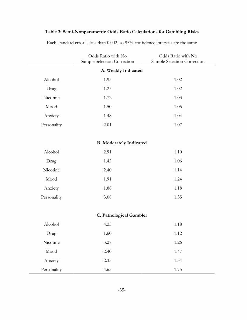
Table 3: Semi-Nonparametric Odds Ratio Calculations for Gambling Risks

Each standard error is less than 0.002, so 95% confidence intervals are the same

Odds Ratio with NoSample Selection Correction

Odds Ratio with NoSample Selection Correction

A. Weakly Indicated

Alcohol 1.95 1.02

Drug 1.25 1.02

Nicotine 1.72 1.03

Mood 1.50 1.05

Anxiety 1.48 1.04

Personality 2.01 1.07

B. Moderately Indicated

Alcohol 2.91 1.10

Drug 1.42 1.06

Nicotine 2.40 1.14

Mood 1.91 1.24

Anxiety 1.88 1.18

Personality 3.08 1.35

C. Pathological Gambler

Alcohol 4.25 1.18

Drug 1.60 1.12

Nicotine 3.27 1.26

Mood 2.40 1.47

Anxiety 2.35 1.34

Personality 4.65 1.75

-35-

-36-

-37-

-38-

-39-

-40-

-41-

References

Abbott, Max W., and Volberg, Rachel, A., Taking the Pulse on Gambling and Problem Gambling in NewZealand: A Report on Phase ONE of the 1999 National Prevalence Survey. New Zealand: Departmentof Internal Affairs, Government of New Zealand, 2000.

Algeria, Analucia A.; Petry, Nancy M.; Hasin, Deborah S.; Liu, Shang-Min; Grant, Bridget F., andBlanco, Carlos, “Disordered Gambling Among Racial and Ethnic Groups in the US: Resultsfrom the National Epidemiologic Survey on Alcohol and Related Conditions,” CNS Spectrums14, 2009, 132-142.

American Psychiatric Association, Diagnostic and Statistical Manual of Mental Disorders III (DSM-III)Washington DC: APA Press, 1980.

American Psychiatric Association, Diagnostic and Statistical Manual of Mental Disorders III Revision(DSM-III-R) Washington DC: APA Press, 1987.

American Psychiatric Association, Diagnostic and Statistical Manual of Mental Disorders IV (DSM-IV)Washington DC: APA Press, 1994.

American Psychiatric Association, Diagnostic and Statistical Manual of Mental Disorders 5 (DSM 5)Washington DC: APA Press, 2013.

Australian Productivity Commission, Australia’s Gambling Industries: Inquiry Report (Canberra: AustralianGovernment Productivity Commission, November 1999).

Bärnighausen, Till; Bor, Jacob; Wandira-Kazibwe, Speciosa, and Canning, David, “Correcting HIVPrevalence Estimates for Survey Nonparticipation Using Heckman-Type Selection Models,”Epidemiology, 22(1), January 2011a, 27-35.

Bärnighausen, Till; Bor, Jacob; Wandira-Kazibwe, Speciosa, and Canning, David, “Interviewer Identityas Exclusion Restriction in Epidemiology,” Epidemiology, 22(3), May 2011b, 446.

Billi, Rosa; Stone, Christine A.; Abbott, Max, and Yeung, Kristal, “The Victorian Gambling Study(VGS): A Longitudinal Study of Gambling and Health in Victoria, 2008–2012: Design andMethods,” International Journal of Mental Health and Addiction, 13, 2015, 274-296.

Billi, Rosa; Stone, Christine A.; Marden, P., and Yeung, Kristal, The Victorian Gambling Study: ALongitudinal Study of Gambling and Health in Victoria, 2008–2012 (Victoria, Australia: VictorianResponsible Gambling Foundation, 2014).

Blaire, Grame; Imai, Kosuke, and Zhou, Yang-Yang, “Design and Analysis of the RandomizedResponse Technique,” Journal of the American Statistical Association, 110(511), September 2015,1304-1319.

Blanco, Carlos; Hasin, Deborah S.; Petry, Nancy; Stinson, Frederick S., and Grant, Bridget F., “Sex

Differences in Subclinical and DSM-IV Pathological Gambling: Results from the NationalEpidemiologic Survey on Alcohol and Related Conditions,” Psychological Medicine, 36, 2006, 943-953.

-42-

Blaszczynski, A.; Dumlao, V., and Lange, M., “‘How Much Do You Spend on Gambling?’ Ambiguitiesin Survey Questionnaire Form,” Journal of Gambling Studies, 13(3), Fall 1977, 237-252.

Chaix, Basile; Bilaudeau, Nathalie; Thomas, Frédérique; Havard, Sabrina; Evans, David; Kestens, Yan,and Bean, Kathy, “Neighborhood Effects on Health: Correcting Bias From NeighborhoodEffects on Participation,” Epidemiology, 22(1), January 2011, 18-26.

Committee on the Social and Economic Impact of Pathological Gambling, Pathological Gambling: ACritical Review Washington: National Academy Press, 1999.

Currie, Shawn R.; Miller, Natalie; Hodgins, David C., and Wang, Jian Li, “Defining a Threshold ofHarm from Gambling for Population Health Surveillance Research,” International GamblingStudies, 9(1), April 2009, 19-38.

De Luca, Giuseppe, “SNP and SML Estimation of Univeriate and Bivariate Binary-Choice Models,”Stata Journal, 8(2), 2008, 190-220.

De Luca, Giuseppe, and Perotti, Valeria, “Estimation of Ordered Response Models with SampleSelection,” Stata Journal, 11(2), 2011, 213-239.

DiNardo, John; McCrary, Justin, and Sanbonmatsu, Lisa, “Constructive Proposals for Dealing withAttrition: An Empirical Example,” NBER Working Paper, July 2006.

Ferris, Jackie, and Wynne, Harold, The Canadian Problem Gambling Index Final Report (Ottawa: CanadianCenter on Substance Abuse, 2001); at www.ccsa.ca/pdf/ccsa-008805-2001.pdf.

Fisher, Susan, “Measuring the Prevalence of Sector-Specific Problem Gambling: A Study of CasinoPatrons,” Journal of Gambling Studies, 16(1), 2000, 25-51.

Friedman, Milton, and Savage, Leonard, “Utility Analysis of Choices Involving Risk,” Journal of PoliticalEconomy, 56(4), 1948, 279-304.

Gainsbury, Sally M.; Russell, Alex, and Blaszczynski, Alex, “Are Psychology University StudentGamblers Representative of Non-university Students and General Gamblers? A ComparativeAnalysis,” Journal of Gambling Studies, 30, 2014, 11-25.

Gallant, A. Ronald, and Douglas W. Nychka, “Semi-Nonparametric Maximum Likelihood Estimation,”Econometrica, 55(2), March 1987, 363–390.

Geneletti, Sara; Mason, Alexina, and Best, Nicky, “Commentary: Adjusting for Selection Effects inEpidemiologic Studies: Why Sensitivity Analysis is the Only ‘Solution’,” Epidemiology, 22(1),January 2011, 36-39.

Genius, Margarita, and Strazzera, Elisabetta, “Applying the Copula Approach to Sample SelectionModelling,” Applied Economics, 40(11), 2008, 1443-1455.

Gerstein, Dean; Hoffman, John; Larison, Cindy; Engelman, Laszlo; Murphy, Sally; Palmer, Amanda;Chucro, Lucian; Tace, Marianna; Johnson, Robert; Buie, Tracy; Hill, Mary Ann; Volberg, Rachel;Harwood, Henrick; Tucker, Adam; Christiansen, Eugene; Cummings, Will, and Sinclair,Sebastian, Gambling Impact and Behavior Study: Report to the National Gambling Impact Study Commission

-43-

(Chicago: National Opinion Research Center at the University of Chicago, 1999).

Harrison, Glenn W.; Jessen, Lasse J.; Lau, Morten, and Ross, Don, “Disordered Gambling Prevalence:Methodological Innovations in a General Danish Population Survey,” CEAR Working Paper2016-04, Center for the Economic Analysis of Risk, Robinson College of Business, GeorgiaState University, 2016.

Harrison, Glenn W., and Lau, Morten, “Risk Attitudes, Sample Selection and Attrition in a LongitudinalField Experiment,” CEAR Working Paper 2014-04, Center for the Economic Analysis of Risk,Robinson College of Business, Georgia State University, 2014.

Harrison, Glenn W., and Ng, Jia Min, “Evaluating the Expected Welfare Gain from Insurance,” Journalof Risk and Insurance, 83(1), 2016, 91-120.

Heckman, James J., “The Common Structure of Statistical Models of Truncation, Sample Selection andLimited Dependent Variables and a Simple Estimator for Such Models,” Annals of Economic andSocial Measurement, 1976, 5, 475–492.

Heckman, James J., “Sample Selection Bias as a Specification Error,” Econometrica, 47(1), January 1979,153-162.

Hernán, Miguel A.; Hernández-Diaz, Sonia, and Robins, James M., “A Structural Approach to SelectionBias,” Epidemiology, 15(5), September 2004, 615-625.

Kessler, Ronald C; Abelson, Jamie; Demler, Olga; Escobar, Javier I.; Gibbon, Miriam; Guyer, MargaretE.; Howes, Mary J.; Jin, Robert; Vega, William A.; Walters, Ellen E.; Wang, Phillip; Zaslavsky,Alan, and Zheng, Hui, “Clinical calibration of DSM-IV diagnoses in the World Mental Health(WMH) version of the World Health Organization (WHO) Composite International DiagnosticInterview (WMH-CIDI),” International Journal of Methods in Psychiatric Research, 13(2), 2004, 122-139.

Kessler, R.C.; Hwang, I.; LaBrie, R.; Petukhova, M.; Sampson, N.A.; Winters, K.C., and Shaffer, H.J.,“DSM-IV Pathological Gambling in the National Comorbidity Survey Replication,” PsychologicalMedicine, 38, 2008, 1351-1360.

Kessler, Ronald C., and Pennell, Beth-Ellen, “Developing and Selecting Mental Health Measures,” inT.P. Johnson (ed.), Handbook of Health Survey Methods (New York: Wiley, 2015).

Lee, Lung-Fei, “Generalized Econometric Models with Selectivity,” Econometrica, 51, 1983, 507-512.

Lesieur, Henry R., “Epidemiological Surveys of Pathological Gambling: Critique and Suggestions forModification,” Journal of Gambling Studies, 10(4), 1994, 385-398.

Lesieur, Henry R., and Blume, Sheila B., “The South Oaks Gambling Screen (SOGS): A NewInstrument for the Identification of Pathological Gamblers,” American Journal of Psychiatry, 144(9),September 1987, 1184-1188.

Lesieur, Henry R.; Blume, Sheila B., and Zoppa, Richard M., “Alcoholism, Drug Abuse, and Gambling,”Alcoholism: Clinical and Experimental Research, 10(1), January 1986, 33-38.

-44-

Maddala, G. S., Limited-Dependent and Qualitative Variables in Econometrics (New York: CambridgeUniversity Press, 1983).

Narrow, William E.; Rae, Donald S.; Robins, Lee N, and Reiger, Darrel A., “Revised PrevalenceEstimates of Mental Disorders in the United States: Using a Clinical Significance Criterion toReconcile 2 Surveys’ Estimates,” Archives of General Psychiatry, 59, 2002, 115-123.

Nower, Lia; Martins, Silvia; Lin, Keng-Han, and Blanco, Carlos, “Subtypes of Disordered Gamblers:

Results from the National Epidemiologic Survey on Alcohol and Related Conditions,” Addiction108(4), 2013, 789-798.

Omnifacts Research, “An Examination of the Prevalence of Gambling in Nova Scotia,” Report #93090,Nova Scotia Department of Health, May 1993; available athttp://dspace.ucalgary.ca/jspui/handle/1880/48485

Orr, Larry; Feins, Judith D. Feins; Jacob, Robin; Beecroft, Erik; Sanbonmatsu, Lisa; Katz, Lawrence F.;Liebman, Jeffrey B., and Kling, Jeffrey R., “Moving to Opportunity Interim ImpactsEvaluation,” Final Report, U.S. Department of Housing and Urban Development, 2003.

Petry, Nancy; Blanco, Carlos; Jin, Chelsea, and Grant, Bridget F., “Concordance Between GamblingDisorder Diagnoses in the DSM-IV and DSM-5: Results from the National EpidemiologicSurvey on Alcohol and Related Disorders [sic],” Psychology of Addictive Behaviors, 28(2), 2014, 586-591.

Pietrzak, Robert H.; Morasco, Banjamin J.; Blanco, Carlos; Grant, Bridget F., and Petry, Nancy M.,“Gambling Level and Psychiatric and Medical Disorders in Older Adults: Results from theNational Epidemiologic Survey on Alcohol and Related Conditions,” American Journal of GeriatricPsychiatry 15, 2007, 301-313.

Rachlin, Howard, “Why Do People Gamble and Keep Gambling Despite Heavy Losses?” PsychologicalScience, 1, 1990, 294-297.

Rachlin, Howard, The Science of Self-Control (Cambridge, MA: Harvard University Press, 2000).

Rachlin, Howard; Safin Vasiliy; Arfer, Kodi B., and Yen, Ming, “The Attraction of Gambling,” Journal ofthe Experimental Analysis of Behavior, 103(1), January 2015, 260-266.

Ross, Don; Sharp, Carla; Vuchinich, Rudy, and Spurrett, David, Midbrain Mutiny: The Picoeconomics andNeuroeconomics of Disordered Gambling (Cambridge, MA: MIT Press, 2008).

Rothman, Kenneth J.; Greenland, Sander, and Lash, Timothy, L., Modern Epidemiology (New York:Lippincott, Williams & Wilkin, 3rd Edition, 2012).

Schellinck, Tony; Schrans, Tracy; Bliemel, Michael, and Schellinck, Heather, “Construct Developmentfor the FocaL Adult Gambling Screen (FLAGS): A Risk Measurement for Gambling Harm andProblem Gambling Associated with Electronic Gambling Machines,” Journal of Gambling Issues,2015a, 140-173.

Schellinck, Tony; Schrans, Tracy; Bliemel, Michael, and Schellinck, Heather, “Instrument Developmentfor the FocaL Adult Gambling Screen (FLAGS-EGM): A Measurement of Risk and Problem

-45-

Gambling Associated with Electronic Gambling Machines,” Journal of Gambling Issues, 2015b,174-200.

Schwartz, David G., United States Commercial Casino Revenues Las Vegas: Center for Gaming Research,University Libraries, University of Nevada Las Vegas, 2016.

Schüll, Natasha Dow, Addiction By Design: Machine Gambling in Las Vegas (Princeton: Princeton UniversityPress, 2012).

Sharp, Carla; Steinberg, Lynne; Yaroslavsky, Ilya; Hofmeyr, Andre; Dellis, Andrew; Ross, Don, and

Kincaid, Harold, “An Item Response Theory Analysis of the Problem Gambling SeverityIndex,” Assessment, 19(2), 2012, 167-175.

Smith, Murray D., “Modelling Sample Selection Using Archimedian Copulas,” The Econometrics Journal,6(1), 2003, 99-123.

StataCorp, Stata Base Reference Manual: Version 13 (College Station, TX: StataCorp LP, 2013).

Statistics Canada, Health Statistics Division, Canadian Community Health Survey. Cycle 1.2: Mental Health andWell-Being (Ottawa: Statistics Canada, September 2004, Catalogue #82M0021GPE).

Stewart, Mark B., “Semi-nonparametric Estimation of Extended Ordered Probit Models,” Stata Journal,

4(1), 2004, 27-39.

Stewart, Mark B., “A Comparison of Semiparametric Estimators for the Ordered Response Model,”Computational Statistics & Data Analysis, 49, 2005, 555-573.

Stone, Christine; Romild, Ulla; Abbott, Max; Young, Kristal; Billi, Rosa, and Volberg, Rachel, “Effectsof Different Screening and Scoring Thresholds on PGSI Gambling Risk Segments,” InternationalJournal of Mental Health and Addiction 13, 2015, 82-102.

Tax Policy Center, State & Local Government Finance Data Query System The Urban Institute-BrookingsInstitution Tax Policy Center; http://slfdqs.taxpolicycenter.org/pages.cfm; date of Access: June20, 2016.

Toce-Gerstein, Marianna; Gerstein, Dean, and Volberg, Rachel, “A Hierarchy of Gambling Disorders inthe Community,” Addiction, 98, 2003, 1661-1672.

van Hasselt, Martijn, “Bayesian Inference in a Sample Selection Model,” Journal of Econometrics, 165, 1011,221-232.

Van de Ven, Wynand P.M.M., and Van Praag, Bernard M.S., “The Demand for Deductibles in Private

Health Insurance: A Probit Model with Sample Selection,” Journal of Econometrics, 17, 1981, 229-252.

Volberg, Rachel A., “Prevalence Studies of Problem Gambling in the United States,” Journal of GamblingStudies, 12(2), Summer 1996, 111-128.

Volberg, Rachel A., and Steadman, Henry J., “Refining Prevalence Estimates of PathologicalGambling,” American Journal of Psychiatry, 145(4), April 1988, 502-505.

-46-

Volberg, Rachel A., and Steadman, Henry J., “Prevalence Estimates of Pathological Gambling in NewJersey and Maryland,” American Journal of Psychiatry, 146(12), December 1989, 1618-1619.

Volberg, Rachel A., and Williams, Robert J., “Developing a Short Form of the PGSI,” Report to theGambling Commission (Northampton, MA: Gemini Research, January 2012); available athttp://www.gamblingcommission.gov.uk/pdf/Developing a Short Form of the PGSI.pdf.

Walker, Douglas, Casinonomics (Berlin: Springer, 2013).

Walker, Michael B., and Dickerson, Mark G., “The Prevalence of Problem and Pathological Gambling:A Critical Analysis,” Journal of Gambling Studies, 12(2), 1996, 233-249.

Wardle, Heather; Moody, Alison; Spence, Suzanne; Orford, Jim; Volberg, Rachel; Jotangia, Dhriti;Griffiths, Mark; Hussey, David, and Dobbie, Fiona, British Gambling Prevalence Survey 2010(London, UK: National Centre for Social Research, 2011).

Warner, Stanley L., “Randomized Response: A Survey Technique for Eliminating Evasive Answer Bias,”Journal of the American Statistical Association, 60(309), March 1965, 63-69.

Williams, Robert J., and Volberg, Rachel, “Impact of survey description, administration format, andexclusionary criteria on population prevalence rates of problem gambling,” International GamblingStudies, 9(2), 2009, 101-117.

Williams, Robert J., and Volberg, Rachel A., “Best practices in the population assessment of problemgambling,” Report (Guelph: Ontario Problem Gambling Research Centre, March 2010); availableat https://www.uleth.ca/dspace/handle/10133/1259.

Williams, Robert J.; Volberg, Rachel A., and Stevens, Rhys M.G., “The Population Prevalence ofProblem Gambling: Methodological Influences, Standardized Rates, Jurisdictional Differences,and Worldwide Trends,” Report Prepared for the Ontario Problem Gambling Research Centre & theOntario Ministry of Health and Long Term Care, May 2012; available atwww.gamblingresearch.org/applydownload.php?docid=12579?.

Williams, Robert J., and Wood, Robert T., “The Proportion of Gambling Revenue Derived fromProblem Gamblers: Examining the Issues in a Canadian Context,” Analyses of Social Issues andPublic Policy, 4(1), 2004, 33-45.

Wood, Robert T., and Williams, Robert J., “‘How Much Money Do You Spend on Gambling?’ The

Comparative Validity of Question Wordings Used to Assess Gambling Expenditure,”International Journal of Social Research Methodology, 10(1), February 2007, 63-77.

Zuehlke, Thomas W., and Zeman, Allen R., “A Comparison of Two-Stage Estimators of CensoredRegression Models,” Review of Economics & Statistics, 73(1), February 1991, 185-188.

-47-

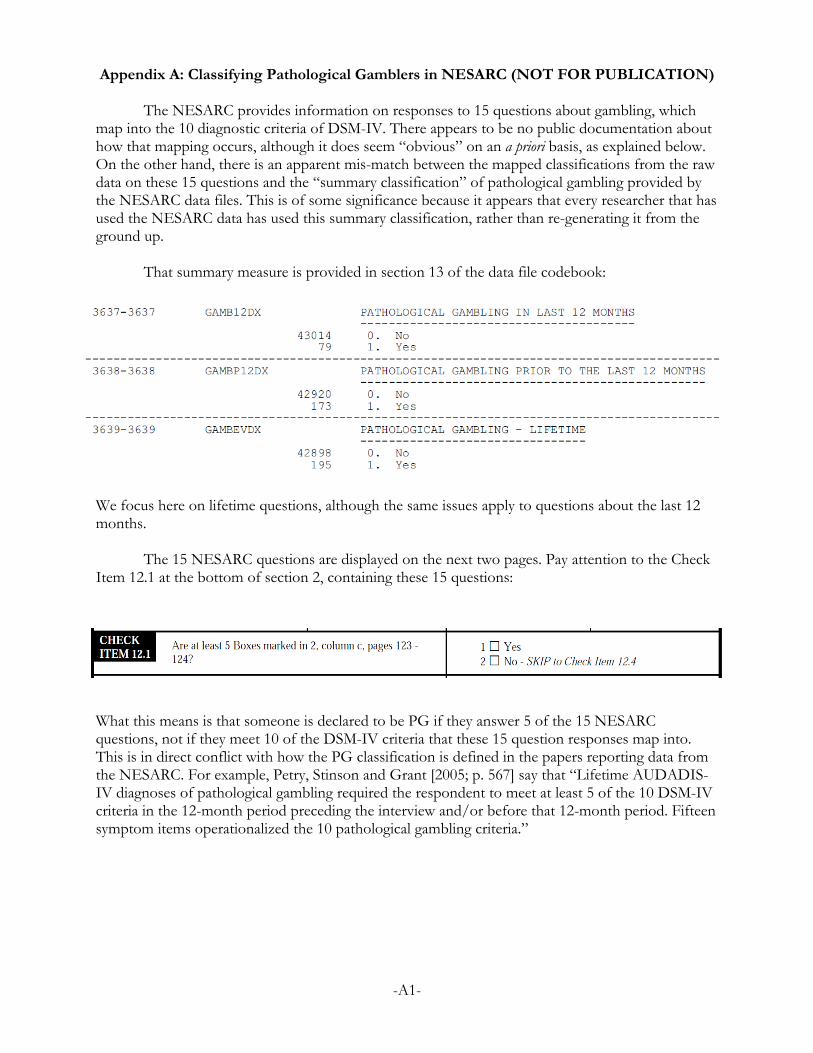
Appendix A: Classifying Pathological Gamblers in NESARC (NOT FOR PUBLICATION)

The NESARC provides information on responses to 15 questions about gambling, whichmap into the 10 diagnostic criteria of DSM-IV. There appears to be no public documentation abouthow that mapping occurs, although it does seem “obvious” on an a priori basis, as explained below.On the other hand, there is an apparent mis-match between the mapped classifications from the rawdata on these 15 questions and the “summary classification” of pathological gambling provided bythe NESARC data files. This is of some significance because it appears that every researcher that hasused the NESARC data has used this summary classification, rather than re-generating it from theground up.

That summary measure is provided in section 13 of the data file codebook:

We focus here on lifetime questions, although the same issues apply to questions about the last 12months.

The 15 NESARC questions are displayed on the next two pages. Pay attention to the CheckItem 12.1 at the bottom of section 2, containing these 15 questions:

What this means is that someone is declared to be PG if they answer 5 of the 15 NESARCquestions, not if they meet 10 of the DSM-IV criteria that these 15 question responses map into.This is in direct conflict with how the PG classification is defined in the papers reporting data fromthe NESARC. For example, Petry, Stinson and Grant [2005; p. 567] say that “Lifetime AUDADIS-IV diagnoses of pathological gambling required the respondent to meet at least 5 of the 10 DSM-IVcriteria in the 12-month period preceding the interview and/or before that 12-month period. Fifteensymptom items operationalized the 10 pathological gambling criteria.”

-A1-

-A2-

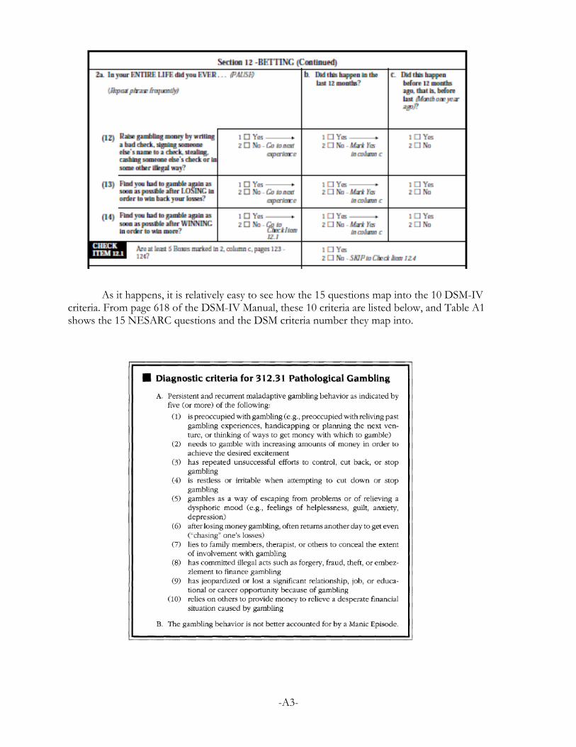
As it happens, it is relatively easy to see how the 15 questions map into the 10 DSM-IVcriteria. From page 618 of the DSM-IV Manual, these 10 criteria are listed below, and Table A1shows the 15 NESARC questions and the DSM criteria number they map into.

-A3-

Table A1: Mapping from 15 NESARC Gambling Criteria to 10 DSM-IV Criteria

NESARC Gambling Questions DSM Criteria

(1) Gamble to get out of a bad mood – like feeling nervous, sad or down? 5

(2) Gamble to forget your problems? 5

(3) More than once try to quit or cut down on your gambling, but foundyou couldn’t do it?

3

(4) Find that you had to increase the amount of money you would gambleto keep it exciting?

2

(5) Spend a lot of time gambling, planning your bets or studying theodds?

1

(6) Spend a lot of time thinking about ways to get money together so youcould gamble?

1

(7) Spend a lot of time thinking about the times when you won or lost? 1

(8) Have job or school trouble because of your gambling – like missingtoo much work, being demoted at work, losing your job ordropping out of school?

9

(8a) Break up or come close to breaking up with anyone who wasimportant to you because of your gambling?

9

(9) Try to keep your family or friends from knowing how much yougamble?

7

(10) Have such financial trouble as a result of your gambling that you hadto get help with living expenses from family, friends or welfare?

10

(11) Find that you become restless, irritable or anxious when trying toquit or cut down in your gambling?

4

(12) Raise gambling money by writing a bad check, signing someoneelse’s name to a check, stealing, cashing someone else’s check orin some other illegal way?

8

(13) Find that you had to gamble again as soon as possible after LOSINGin order to win back your losses?

6

(14) Find that you had to gamble again as soon as possible afterWINNING in order to win more?

2

-A4-

If one undertakes this mapping for each individual in the survey, there are actually 207 PGsubjects in these data, not 195 as tabulated in section 14 of the data. Here is a tabulation:

Number of | PG DSM-IV | criteria | pg_lifetime met | 0 Yes | Total-----------+----------------------+---------- 0 | 40,814 0 | 40,814 1 | 1,251 0 | 1,251 2 | 448 0 | 448 3 | 257 0 | 257 4 | 107 9 | 116 5 | 19 59 | 78 6 | 1 42 | 43 7 | 1 39 | 40 8 | 0 28 | 28 9 | 0 13 | 13 10 | 0 5 | 5 -----------+----------------------+---------- Total | 42,898 195 | 43,093

We see that 9 individuals were incorrectly defined to be PG when they only met 4 of the DSM-IVcriteria, but that 21 individuals were defined as not being PG when they did indeed meet 5 or moreof the DSM-IV. We do not know that all of these 21 were incorrectly defined, since we need to decidewhether or not to check the DSM-IV exclusionary criterion, that they did not suffer from ManicEpisodes.

As it happens, the NESARC has information on that criteria, and 3 of these 21 did exhibitsuch Manic Episodes if we choose to implement this exclusionary criteria using these NESARCdata. We do not rule out cases associated with recent illness or bereavement. If we drop anyone withsuch episodes, we see something more problematic:

. tab pg_dsm_count pg_lifetime if manic_episodes==0, missing

Number of | PG DSM-IV | criteria | pg_lifetime met | 0 Yes | Total-----------+----------------------+---------- 0 | 39,515 0 | 39,515 1 | 1,159 0 | 1,159 2 | 401 0 | 401 3 | 218 0 | 218 4 | 92 5 | 97 5 | 16 45 | 61 6 | 1 33 | 34 7 | 1 29 | 30 8 | 0 19 | 19 9 | 0 9 | 9 10 | 0 2 | 2 -----------+----------------------+---------- Total | 41,403 142 | 41,545

-A5-

In other words, many of the 195 originally classified as PG should have been excluded. Specifically,53 subjects:

. tab pg_lifetime manic_episodes, missing

pg_lifetim | manic_episodes e | 0 1 | Total-----------+----------------------+---------- 0 | 41,403 1,495 | 42,898 Yes | 142 53 | 195 -----------+----------------------+---------- Total | 41,545 1,548 | 43,093

We do not endorse this way of implementing the DSM-IV exclusionary criteria, but simply note herethe consequences for sample size.

The hypothesis about what was done to generate the summary measure of PG that appearsto have been used by all researchers using NESERC is confirmed if one does a “count” of thenumber of NESARC questions answered affirmatively:

. tab pg_count pg_lifetime, missing

Number of | PG NESARC | criteria | pg_lifetime met | 0 Yes | Total-----------+----------------------+---------- 0 | 40,814 0 | 40,814 1 | 1,066 0 | 1,066 2 | 486 0 | 486 3 | 257 0 | 257 4 | 133 0 | 133 5 | 77 12 | 89 6 | 46 29 | 75 7 | 13 35 | 48 8 | 5 30 | 35 9 | 1 27 | 28 10 | 0 18 | 18 11 | 0 21 | 21 12 | 0 12 | 12 13 | 0 5 | 5 14 | 0 3 | 3 15 | 0 3 | 3 -----------+----------------------+---------- Total | 42,898 195 | 43,093

So we see that an individual was only classified as being PG in the summary measure if they had 5 ofthe 15 NESARC criteria. The fact that researchers used this summary measure is apparent frominspection of the reported sample size of 195 PG (e.g., Petry et al. [2005; Table 1, p. 568] or Blancoet al. [2006; Table 1, p.947]).

On the other hand, the above tabulation poses a puzzle, since there are many individualswith 5 or more of the 15 NESARC criteria that are not classified as PG. In fact, there are77+46+13+5+1 = 142 such individuals. It is not as if these 142 individuals met some of theNESARC criteria that do not map into DSM criteria, since the NESARC criteria that they meet spanall 15 NESARC questions. There appears to have been some algorithm used to defined PG in thesummary measure that is not documented. For this reason we prefer to re-generate our ownmeasure of PG using the DSM-IV criteria.

There are 207 correct DSM-IV based PG individuals in the NESARC:

-A6-

. tab pg_dsm_correct pg_lifetime, missing

Correct | DSM-IV | criteria |applied to | NESARC | data for | pg_lifetime lifetime | 0 Yes | Total-----------+----------------------+---------- 0 | 42,877 9 | 42,886 1 | 21 186 | 207 -----------+----------------------+---------- Total | 42,898 195 | 43,093

There have been some variants of the DSM-IV threshold criteria applied in some research.For instance, as noted in the text, Fisher [2000] prefers the term “problem” to “pathological”outside of a shared, clinical diagnosis, and then (p. 33) defines problem gamblers using either 5 ormore “yes” responses to the DSM-IV criteria or 3 or 4 “yes” responses that include at least one fromitems 8, 9 or 10 of the criteria. These last three refer to the adverse consequences of gambling. Thisdefinition can only logically increase the number of “classified” gamblers compared to the use of 5or more “yes” responses. In fact, for the NESARC data this results in 256 “classified” gamblerscompared to the 207 correct DSM-IV PG individuals:

. tab pg_dsm_correct_extra, missing

pg_dsm_corr | ect_extra | Freq. Percent Cum.------------+----------------------------------- 0 | 42,837 99.41 99.41 1 | 256 0.59 100.00------------+----------------------------------- Total | 43,093 100.00

. tab pg_dsm_correct_extra pg_dsm_correct, missing

| Correct DSM-IV | criteria applied to | NESARC data forpg_dsm_cor | lifetimerect_extra | 0 1 | Total-----------+----------------------+---------- 0 | 42,837 0 | 42,837 1 | 49 207 | 256 -----------+----------------------+---------- Total | 42,886 207 | 43,093

It is also worthwhile doing the correct analysis using the DSM-V criteria. The new criteriadrop the “illegal acts” question, and require that only 4 criteria be met. In this respect we mimic theapproach of Petryy, Blanco, Jon and Grant [2014] to “re-cycling” the NESARC data in this manner:

. tab pg_dsm5_correct pg_lifetime, missing

Correct | DSM-V | criteria |applied to | NESARC | pg_lifetime data | 0 Yes | Total-----------+----------------------+---------- 0 | 42,772 0 | 42,772 1 | 126 195 | 321 -----------+----------------------+----------

-A7-

Total | 42,898 195 | 43,093

So we now have 321 individuals with PG, using the DSM-V criteria.

We contacted researchers that have used NESARC to find out if there is some simpleexplanation for our finding of an error in the coding of PG. We keep their identity anonymous, forreasons that will become apparent.

One responded:

Yes, NESARC is not easy to navigate. There are some sort of weights you need toadd to the calculations, to weight by baseline characteristics because some subgroupswere oversampled for the survey. I have not done this in many years, and no longerhave the syntax. I believe they are described in many of the NESARC papers, aseverybody appears to use these weights. My guess is that is what is incorrect, ratherthan how you’re coding the DSM criteria, which is more straightforward. In any case,I’m certain the numbers reported in the 2005 paper are correct, because manysubsequent papers have been written about the PGs in that dataset, and no one’sreported difficulty replicating the n’s or analyses. I am not a statistician, but there area lot of statisticians who are experienced at NESARC analyses and could probablyhelp.

In fact, we find NESARC relatively straightforward to navigate, and it is well documented apartfrom this apparent coding error. The use of survey weights, which we are aware of and use forappropriate tabulations (e.g., prevalence and odd ratio estimation), is not the issue since this refers tothe raw sample count reported in published papers. The final point, that we should trust thateveryone else that has used the data has checked this, is not germane to a scholarly evaluation ofthese data. There is a simple error or there is not.

A second researcher, a statistician and experienced at NESARC analysis, then responded:

I have read your attachment and have 2 initial comments that might help resolve thisissue. First the skip item is only used during the interview to decide whether to askadditional pg questions and does not come into play with regard to creatingdiagnoses. Second we never use the ever columns to determine diagnoses. We usethe 12 month and prior to the 12 month columns only and if positive for any ofthose 2 time frames we declare a lifetime diagnosis. If this does not resolve yourissues please let me know so I can examine them more closely.

The first point, about the skip question, is irrelevant to the issue. The second point is worthchecking, and would arise from some inconsistency between reports made by the same individualabout the same NESARC criteria. In fact, however, if one reviews the earlier extract from thequestions involved, it is apparent that consistency here is enforced if the interviewer followed the logicof the skip pattern correctly.40 There are 4 such inconsistencies. In 3 of these 4 there was a positive

40 NESARC criteria #1 is asked on a lifetime basis. If the response is NO then the 12-month andbefore 12-month responses are left missing, which consistently implies a NO for lifetime. If the response tothe direct lifetime question is YES then the “last 12 months” question is asked. If there is a YES to the “last12 months” question then the “before 12 months” question is asked, and whatever the response to thatquestion we have consistency. If there is a NO to the “last 12 months” question then the “before 12 months”

-A8-

responses to the direct lifetime question, but both the “last 12 months” and “before the last 12months” are left blank; perhaps the respondent said that they could not be bothered with the follow-up. In 1 of these 4 the “last 12 months” was left blank but the “before 12 months” was marked NO.This cannot be the cause of the discrepancy we are pointing out.

question is automatically filled in as a YES to ensure consistency.

-A9-

Appendix B: Additional Documentation of Results (NOT FOR PUBLICATION)

All variables are defined from the original data files of wave 1 of the NESARC, and Statacode explaining the detailed definitions is available on request. The variables are as follows:

variable name variable label-----------------------------------------------------------------------------------pg_dsm_correct Correct DSM-IV criteria applied to NESARC data for lifetime

alcohol Any lifetime alcohol disorderdrug Any lifetime drug use disordernicotine Any lifetime nicotine disordermood Any mood disorderanxiety Any anxiety disorderpersonality Any personality disorder

female Femaleblack Black or Afro-Americanhispanic Hispanicage30_44 Aged between 30 and 44age45_64 Aged between 45 and 64age65plus Aged 65 and overseparated Separated by being widowed, divorced or separatedmidwest Midwest regionsouth South regionwest West regionhigh_school Completed High School or GEDsome_college Completed some collegecollege Completed a college degreegraduate Completed a graduate degreeincome2 Personal income between $20,000 and $35,000income3 Personal income between $35,000 and $70,000income4 Personal income of $70,000 or more

height Height in feetweigh Weight in stones

friday Interview conducted on a Fridaysaturday Interview conducted on a Saturdaysunday Interview conducted on a Sunday

pg_Ntriggers Number of triggers activated when pg trigger question asked

personality_battery1 Responses to questions on usual feelings and actionspersonality_battery2 Responses to questions on effects of feelings and actions

ss_1 Sample Selection variable 1 from Screening Question #18 Part 1ss_2 Sample Selection variable 2 from Screening Question #18 Part 2ss_3 Sample Selection variable 3 from Screening Question #19 Part 1ss_4 Sample Selection variable 4 from Screening Question #19 Part 2ss_5 Sample Selection variable 5 from Screening Question #20ss_6 Sample Selection variable 6 from Screening Question #21 Part 1ss_7 Sample Selection variable 7 from Screening Question #21 Part 2ss_8 Sample Selection variable 8 from Screening Question #21 Part 3ss_9 Sample Selection variable 9 from Screening Question #22ss_10 Sample Selection variable 10 from Screening Question #23 Part 1ss_11 Sample Selection variable 11 from Screening Question #23 Part 2ss_12 Sample Selection variable 12 from Screening Question #23 Part 3ss_13 Sample Selection variable 13 from Screening Question #23 Part 4ss_14 Sample Selection variable 14 from Screening Question #23 Part 5ss_15 Sample Selection variable 15 from Screening Question #23 Part 6ss_16 Sample Selection variable 16 from Screening Question #23 Part 7ss_17 Sample Selection variable 17 from Screening Question #23 Part 8ss_18 Sample Selection variable 18 from Screening Question #23 Part 9

-A10-

ss_19 Sample Selection variable 19 from Screening Question #23 Part 10ss_20 Sample Selection variable 20 from Screening Question #23 Part 11ss_21 Sample Selection variable 21 from Screening Question #23 Part 12

-----------------------------------------------------------------------------------

Summary statistics are as follows:

Variable | Obs Mean Std. Dev. Min Max-------------+---------------------------------------------------------pg_dsm_cor~t | 43,093 .0046875 .0683057 0 1-------------+--------------------------------------------------------- alcohol | 43,093 .2748242 .4464308 0 1 drug | 43,093 .0944005 .2923885 0 1 nicotine | 43,093 .1609774 .3675144 0 1 mood | 43,093 .2111944 .4081607 0 1 anxiety | 43,093 .1732764 .3784904 0 1 personality | 43,093 .1460794 .3531899 0 1-------------+--------------------------------------------------------- female | 43,093 .5702782 .4950421 0 1 black | 43,093 .1995684 .3996806 0 1 hispanic | 43,093 .1927923 .394496 0 1 age30_44 | 43,093 .3105377 .4627191 0 1 age45_64 | 43,093 .2979602 .4573672 0 1 age65plus | 43,093 .1904022 .3926229 0 1 separated | 43,093 .2579769 .4375263 0 1 midwest | 43,093 .2086418 .4063425 0 1 south | 43,093 .3749101 .4841053 0 1 west | 43,093 .2259532 .4182133 0 1 high_school | 43,093 .291161 .4543028 0 1some_college | 43,093 .2063212 .4046685 0 1 college | 43,093 .2093844 .4068739 0 1 graduate | 43,093 .1109925 .3141265 0 1 income2 | 43,093 .2314761 .4217808 0 1 income3 | 43,093 .2095236 .4069733 0 1 income4 | 43,093 .2906969 .4540892 0 1-------------+--------------------------------------------------------- height | 43,093 5.549293 .3356052 4 7 weigh | 43,093 12.17406 2.914927 4.428571 35.71429 friday | 43,093 .1413919 .3484294 0 1 saturday | 43,093 .1438981 .3509904 0 1 sunday | 43,093 .0768106 .2662938 0 1-------------+---------------------------------------------------------pg_Ntriggers | 43,093 .1886385 .7641052 0 7-------------+---------------------------------------------------------personalit~1 | 43,093 3.466642 4.772873 0 55personalit~2 | 43,093 3.443552 4.769596 0 55-------------+--------------------------------------------------------- ss_1 | 43,093 .348154 .4763907 0 1 ss_2 | 43,093 .3008841 .4586477 0 1 ss_3 | 43,093 .2764718 .4472581 0 1 ss_4 | 43,093 .2422435 .4284459 0 1 ss_5 | 43,093 .3640963 .4811814 0 1 ss_6 | 43,093 .76256 .425519 0 1 ss_7 | 43,093 .7989697 .4007753 0 1 ss_8 | 43,093 .4865291 .4998243 0 1 ss_9 | 43,093 .2665166 .4421426 0 1 ss_10 | 43,093 .3197503 .4663851 0 1 ss_11 | 43,093 .3476435 .4762276 0 1 ss_12 | 43,093 .1458938 .3530038 0 1 ss_13 | 43,093 .0624463 .2419673 0 1 ss_14 | 43,093 .0896897 .2857401 0 1 ss_15 | 43,093 .079224 .2700912 0 1 ss_16 | 43,093 .2083633 .4061427 0 1 ss_17 | 43,093 .0647437 .2460759 0 1

-A11-

ss_18 | 43,093 .0561576 .2302285 0 1 ss_19 | 43,093 .1168867 .321289 0 1 ss_20 | 43,093 .0552526 .2284753 0 1 ss_21 | 43,093 .0641636 .2450469 0 1-------------+---------------------------------------------------------

The sample selection screening questions come from the “Background Information” sectionof the NESARC questionnaire, reproduced below.

-A12-

-A13-

Figures B1, B2 and B3 show distributions of the predicted marginal probabilities of eachgambling disorder category for the DSM-IV screen from the British Gambling Prevalence Survey of2010, the PGSI screen of the Victorian Gambling Survey of 2008, and the NODS screen of theVictorian Gambling Survey of 2008. In some cases the horizontal axes include labels forprobabilities below 0 or above 1: this is an artefact of the kernel density procedure used to displaydistributions as well as the use of the “delta method” to approximate non-linear combinations ofestimated parameters. These are of no substantive or statistical significance for our purposes.

-A14-

-A15-

-A16-

-A17-