fault diagnosis for satellite sensors and actuators using
TRANSCRIPT

General rights Copyright and moral rights for the publications made accessible in the public portal are retained by the authors and/or other copyright owners and it is a condition of accessing publications that users recognise and abide by the legal requirements associated with these rights.
Users may download and print one copy of any publication from the public portal for the purpose of private study or research.
You may not further distribute the material or use it for any profit-making activity or commercial gain
You may freely distribute the URL identifying the publication in the public portal If you believe that this document breaches copyright please contact us providing details, and we will remove access to the work immediately and investigate your claim.
Downloaded from orbit.dtu.dk on: Mar 23, 2022
Fault Diagnosis for Satellite Sensors and Actuators using Nonlinear GeometricApproach and Adaptive Observers
Baldi, P.; Blanke, Mogens; Castaldi, P.; Mimmo, N.; Simani, S.
Published in:International Journal of Robust and Nonlinear Control
Link to article, DOI:10.1002/rnc.4083
Publication date:2018
Document VersionPeer reviewed version
Link back to DTU Orbit
Citation (APA):Baldi, P., Blanke, M., Castaldi, P., Mimmo, N., & Simani, S. (2018). Fault Diagnosis for Satellite Sensors andActuators using Nonlinear Geometric Approach and Adaptive Observers. International Journal of Robust andNonlinear Control, 5429–5455. https://doi.org/10.1002/rnc.4083

Fault Diagnosis for Satellite Sensors and Actuators usingNonlinear Geometric Approach and Adaptive Observers
P. Baldi1∗, M. Blanke2, P. Castaldi1, N. Mimmo1 and S. Simani3
1Dipartimento di Ingegneria dell’Energia Elettrica e dell’Informazione, Universita di Bologna, Facolta di IngegneriaAerospaziale. 47100 Forlı(FC), Italy.
2Department of Electrical Engineering, Technical University of Denmark, 2800 Kgs. Lyngby, Denmark.3Dipartimento di Ingegneria, Universita di Ferrara. 44123 Ferrara (FE), Italy.
SUMMARY
This paper presents a novel scheme for diagnosis of faults affecting sensors that measure the satellite attitude,body angular velocity, flywheel spin rates, and defects in control torques from reaction wheel motors. Theproposed methodology uses adaptive observers to provide fault estimates that aid detection, isolation andestimation of possible actuator and sensor faults. The adaptive observers do not need a-priori informationabout fault internal models. A nonlinear geometric approach is used to avoid that aerodynamic disturbancetorques have unwanted influence on the fault estimates. An augmented high fidelity spacecraft model isexploited during design and validation to replicate faults. This simulation model includes disturbance torquesas experienced in low Earth orbits. The paper includes an analysis to assess robustness properties of themethod with respect to parameter uncertainties and disturbances. The results document the efficacy of thesuggested methodology.
Received . . .
KEY WORDS: fault diagnosis; nonlinear geometric approach; adaptive observer; structural analysis;actuators and sensors.
1. INTRODUCTION
The increasing operational requirements for onboard autonomy in satellite control systems implyan inherent need for structural methods that support the design of complete and reliable supervisorysystems. It is necessary to design supervision schemes that are capable of realising accuratediagnosis of potential faults, in order to allow subsequent fault accommodation actions to improvesystem reliability and availability, while maintaining desirable performances. In this context, FaultDetection and Diagnosis (FDD) systems provide fundamental information about the health status ofthe system jointly with the estimation of any faults.Significant research in FDD has been done in last three decades [1, 2] and numerous model-basedmethods have been proposed [3, 4]. For a nonlinear spacecraft, linear models fall short, so nonlinearapproaches are needed [5, 6]. The NonLinear Geometric Approach (NLGA) [7] was inspired by theFault Detection and Isolation (FDI) problem for spacecraft. Later research [8, 9, 10] investigatedFDI and FDD methods for spacecraft, and some included supervisory actions to mitigate faults.Specificly, [11] considered faults in reaction wheel control torque and in wheel spin rate sensors,and [12] mapped physical faults to models that were affine with respect to actuator and sensorfaults. The FDI task was carried out, in [11, 13], through cross–checking of residual signals andactuator and sensor fault estimates were provided by dedicated estimation filters using Radial Basis
∗Correspondence to: Dipartimento di Ingegneria dell’Energia Elettrica e dell’Informazione, Universita di Bologna,Facolta di Ingegneria Aerospaziale. 47100 Forlı(FC), Italy. E-mail: [email protected]

2 P. BALDI ET AL.
Function Neural Networks (RBF NN). This approach was quite complex and robustness propertieswere not investigated. The majority of results in spacecraft FDD literature focus on occurrence ofeither actuator or sensor defects separately (se e.g. [14, 15, 16]) or take into account the possibleoccurrence of a more limited number of actuator and sensor faults at the same time, a more holisticview is needed on diagnosis and operability of the entire ADCS.This paper aims to assess the health condition and proper functioning of all essential sensors andactuators used in a spacecraft Attitude Determination and Control System (ADCS). In particular,the sensors measuring the satellite attitude, body angular velocity and flywheel spin rates areconsidered, whereas the actuators are the reaction wheel motors. This work represents a substantialimprovement over previous works of the authors [11, 13]. Reduction in complexity is achieved bya structure where fault estimates from Adaptive Observers (AO) are used as diagnostic signals forall of the fault detection, isolation and estimation tasks. Step-stones in the design are based on thegeneral works [17, 18]. One is to augment models for the design of adaptive observers for sensorfault estimation, such that actual output sensor faults are represented as input signals [19]. Thesecond is the design of adaptive observers for actuator and sensor fault estimation. A third is toemploy the NLGA [7] to obtain diagnostic signals that are independent of the knowledge of theaerodynamic disturbance parameters and decoupled from different subsets of faults. The fourth isto achieve fault isolation through the use of a cross–check of the diagnostic signals and a properdecision logic.Albeit being based on existing theoretical approaches, this paper describes a novel applicationscheme with significant benefits. The joint use of the NLGA and adaptive observers allows totake advantage of the benefits of both of them. The use of adaptive observers allows to designgeneralised fault estimation filters which do not need a priori information about the type of fault.The FDD adaptive observers can accurately estimate a generic fault without needing to define anyspecific fault internal model. The NLGA allows to obtain better FDI performances and accuratefault estimates, independent of the knowledge of the aerodynamic disturbance parameters, andthus without any isolation and estimation error due to aerodynamic parameter uncertainties. TheStructural Analysis (SA) method, which is illustrated in [1] and already suggested for satelliteapplications for example in [20, 21], is exploited to qualitatively assess detectability and isolabilityof faults related to the satellite attitude control system. This satellite–wide analysis of the ADCS willshow that a second physical attitude sensor is required to achieve a complete isolation of possibleattitude and angular velocity sensor faults.The proposed scheme relies on general satellite and reaction wheel dynamic models and a verylimited sensor hardware redundancy, and exploits only sensors and models that are fundamentalfor the ADCS. No additional subsystem models or embedded measurement sensors, e.g. current orvoltage sensors, are required to achieve a complete FDD. Moreover, in practice, it is normal andusually required for safety and reliability reasons to have hardware redundancy available for bothfor satellite actuators and sensor systems.The paper evaluates the performance of the proposed FDD system using a detailed nonlinear satellitesimulator with detailed flywheel modeling [24], measurement noise and exogenous disturbancesignals. In particular, the exogenous disturbance terms are represented by aerodynamic andgravitational disturbance torques. Simulation results show various fault cases. An extensive Monte–Carlo analysis is conducted to assess the robustness and reliability of the proposed diagnosis schemewith respect to parametric uncertainties.The paper is organised as follows. Section 2 describes the overall spacecraft and reaction wheelmodels. Section 3 illustrates the structural analysis of the actuator and sensor fault detectability andisolability. Section 4 illustrates the augmented spacecraft model. Section 5 illustrates the designof the FDD system, which is based on NLGA and adaptive observers. Section 6 illustrates theproposed procedure for the cross-checking of the diagnostic signals and the detection and isolationof the actuator or sensor faults. Section 7 provides simulation results. Concluding remarks are finallydrawn in Section 8.
Manuscript accepted by Int. J. Robust. Nonlinear Control (2018)
SATELLITE FAULT DIAGNOSIS 3
2. SPACECRAFT AND ACTUATOR MODELS
2.1. Dynamic and Kinematic Equations
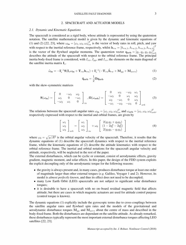
The spacecraft is considered as a rigid body, whose attitude is represented by using the quaternionnotation. The satellite mathematical model is given by the dynamic and kinematic equations of(1) and (2) [22, 23], where ωin = [ω1, ω2, ω3]
Tin is the vector of body rates in roll, pitch, and yaw
with respect to the inertial reference frame, respectively, whilst hrw = [hrw,1, hrw,2, hrw,3, hrw,4]T
is the vector of the flywheel angular momenta. The quaternion vector qorb = [q1, q2, q3, q4]Torb
describes the attitude of the spacecraft with respect to the orbital reference frame. The principalinertia body-fixed frame is considered, with Ixx, Iyy, and Izz , the elements on the main diagonal ofthe satellite inertia matrix Is.
ωin = −I−1s S(Isωin + Trwhrw) + I−1
s (−Trwhrw + Mgg + Maero) (1)
qorb =1
2Ωqorb (2)
with the skew-symmetric matrices
S(ωin) =
0 −ω3 ω2
ω3 0 −ω1
−ω2 ω1 0
in
,Ω(ωorb) =
0 ω3 −ω2 ω1
−ω3 0 ω1 ω2
ω2 −ω1 0 ω3
−ω1 −ω2 −ω3 0
orb
(3)
The relations between the spacecraft angular rates ωin = [ω1, ω2, ω3]Tin and ωorb = [ω1, ω2, ω3]
Torb,
respectively expressed with respect to the inertial and orbital frames, are given by ω1
ω2
ω3
orb
=
ω1
ω2
ω3
in
+ ω0
2(q1q2 + q3q4)(1− 2q2
1 − 2q23)
2(q2q3 − q1q4)
(4)
where ω0 =√µ/R3 is the orbital angular velocity of the spacecraft. Therefore, it results that the
dynamic equations of (1) describe the spacecraft dynamics with respect to the inertial referenceframe, whilst the kinematic equations of (2) describe the attitude kinematics with respect to theorbital reference frame. The inertial and orbital notations for the spacecraft angular velocity andattitude, respectively, will be neglected in the rest of the paper.The external disturbances, which can be cyclic or constant, consist of aerodynamic effects, gravitygradient, magnetic moment, and solar effects. In this paper, the design of the FDD system exploitsthe explicit decoupling only of the aerodynamic torque for the following reasons:
• the gravity is always present and, in many cases, produces disturbance torque at least one orderof magnitude larger than other external torques (e.g. Galileo, Voyager 1 and 2). However, itsmodel is almost perfectly known, and thus its effect does not need to be decoupled;
• many Low Earth Orbit (LEO) spacecrafts are not subject to significant solar disturbancetorques;
• it is desirable to have a spacecraft with no on–board residual magnetic field that affectsattitude; but there are cases in which magnetic actuators are used for attitude control purpose(control torque is known).
The dynamic equations (1) explicitly include the gyroscopic terms due to cross-couplings betweenthe satellite angular rates and flywheel spin rates and the models of the gravitational andaerodynamic disturbance torques Mgg and Maero about the centre of mass and described in thebody-fixed frame. Both the disturbances are dependant on the satellite attitude. As already remarked,these disturbances typically represent the most important external disturbance torques affecting LEOsatellites [22, 23].
Manuscript accepted by Int. J. Robust. Nonlinear Control (2018)
4 P. BALDI ET AL.
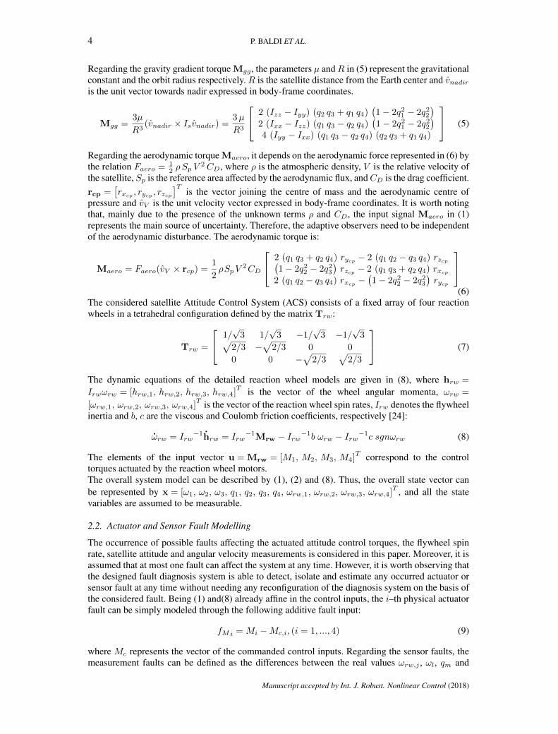
Regarding the gravity gradient torque Mgg, the parameters µ andR in (5) represent the gravitationalconstant and the orbit radius respectively. R is the satellite distance from the Earth center and vnadiris the unit vector towards nadir expressed in body-frame coordinates.
Mgg =3µ
R3(vnadir × Isvnadir) =
3µ
R3
2 (Izz − Iyy) (q2 q3 + q1 q4)(1− 2q2
1 − 2q22
)2 (Ixx − Izz) (q1 q3 − q2 q4)
(1− 2q2
1 − 2q22
)4 (Iyy − Ixx) (q1 q3 − q2 q4) (q2 q3 + q1 q4)
(5)
Regarding the aerodynamic torque Maero, it depends on the aerodynamic force represented in (6) bythe relation Faero = 1
2 ρSp V2 CD, where ρ is the atmospheric density, V is the relative velocity of
the satellite, Sp is the reference area affected by the aerodynamic flux, andCD is the drag coefficient.rcp =
[rxcp
, rycp , rzcp]T
is the vector joining the centre of mass and the aerodynamic centre ofpressure and vV is the unit velocity vector expressed in body-frame coordinates. It is worth notingthat, mainly due to the presence of the unknown terms ρ and CD, the input signal Maero in (1)represents the main source of uncertainty. Therefore, the adaptive observers need to be independentof the aerodynamic disturbance. The aerodynamic torque is:
Maero = Faero(vV × rcp) =1
2ρSpV
2CD
2 (q1 q3 + q2 q4) rycp − 2 (q1 q2 − q3 q4) rzcp(1− 2q2
2 − 2q23
)rzcp − 2 (q1 q3 + q2 q4) rxcp
2 (q1 q2 − q3 q4) rxcp −(1− 2q2
2 − 2q23
)rycp
(6)
The considered satellite Attitude Control System (ACS) consists of a fixed array of four reactionwheels in a tetrahedral configuration defined by the matrix Trw:
Trw =
1/√
3 1/√
3 −1/√
3 −1/√
3√2/3 −
√2/3 0 0
0 0 −√
2/3√
2/3
(7)
The dynamic equations of the detailed reaction wheel models are given in (8), where hrw =
Irwωrw = [hrw,1, hrw,2, hrw,3, hrw,4]T is the vector of the wheel angular momenta, ωrw =
[ωrw,1, ωrw,2, ωrw,3, ωrw,4]T is the vector of the reaction wheel spin rates, Irw denotes the flywheel
inertia and b, c are the viscous and Coulomb friction coefficients, respectively [24]:
ωrw = Irw−1hrw = Irw
−1Mrw − Irw−1b ωrw − Irw−1c sgnωrw (8)
The elements of the input vector u = Mrw = [M1, M2, M3, M4]T correspond to the control
torques actuated by the reaction wheel motors.The overall system model can be described by (1), (2) and (8). Thus, the overall state vector canbe represented by x = [ω1, ω2, ω3, q1, q2, q3, q4, ωrw,1, ωrw,2, ωrw,3, ωrw,4]
T , and all the statevariables are assumed to be measurable.
2.2. Actuator and Sensor Fault Modelling
The occurrence of possible faults affecting the actuated attitude control torques, the flywheel spinrate, satellite attitude and angular velocity measurements is considered in this paper. Moreover, it isassumed that at most one fault can affect the system at any time. However, it is worth observing thatthe designed fault diagnosis system is able to detect, isolate and estimate any occurred actuator orsensor fault at any time without needing any reconfiguration of the diagnosis system on the basis ofthe considered fault. Being (1) and(8) already affine in the control inputs, the i–th physical actuatorfault can be simply modeled through the following additive fault input:
fMi = Mi −Mc,i, (i = 1, ..., 4) (9)
where Mc represents the vector of the commanded control inputs. Regarding the sensor faults, themeasurement faults can be defined as the differences between the real values ωrw,j , ωl, qm and
Manuscript accepted by Int. J. Robust. Nonlinear Control (2018)
SATELLITE FAULT DIAGNOSIS 5
measured values ωrwy,j, ωy,l, qy,m of the j–th flywheel spin rate, l–th satellite angular velocity and
m–th quaternion component, respectively:
fωrw,j = ωrwy,j − ωrw,j (j = 1, ..., 4)fωl
= ωy,l − ωl (l = 1, ..., 3)fqm = qy,m − qm (m = 1, ..., 4)
(10)
It is worth noting that physical attitude sensor faults generally can have an effect on all thecomponents of the provided quaternion vectors simultaneously, thus each physical attitude sensorfault is actually considered as a single additive fault vector fq = [fq1 , fq2 , fq3 , fq4 ]
T affecting themeasurement of the quaternion vector q in the rest of the paper.The presence of fault terms in the output equations of the system does not allow the directexploitation of the NLGA as described in [7]. However, the exploitation of an augmented model, asdescribed in [17] and in the following Section 4, allows to represent the actual output sensor faultsas input faults in the augmented model, and subsequently makes the system model suitable for theexploitation of the NLGA.It is worth noting that in this paper, only additive fault representations are considered, due to therequirement of nonlinear system models affine both in the inputs and faults for the exploitation ofthe Nonlinear Geometric Approach (NLGA). The multiplicative model is, usually, a natural way tomodel a wide variety of sensor and actuator faults, but cannot be used to represent more generalcomponent faults [25]. On the other hand, the additive faults representation is more general than themultiplicative one and can be used to model a wide class of faults, including sensor, actuator, andcomponent faults [25]. In addition, the additive faults representation is more suitable for the designof FDI/FDD schemes because the faults are represented by one signal rather than by changes inthe dynamic model of the system, as is the case with the multiplicative representation. Finally, foractuator faults, the equivalent multiplicative fault magnitude is needed for controller redesign, andthis involves that actuator command is available. However, for actuator fault mitigation, we oftenchoose to disregard actuators with faults and mitigate using remaining healthy actuators. The latterapproach is fully supported by the diagnosis presented in this paper. Multiplicative faults can alwaysbe modelled in an equivalent but additive form. Both additive and multiplicative fault representationscan be equivalently exploited to model a wide variety of abrupt, incipient, intermittent actuator andsensor faults due to different causes (e.g. mechanical, electrical, thermal, magnetic causes, etc.).
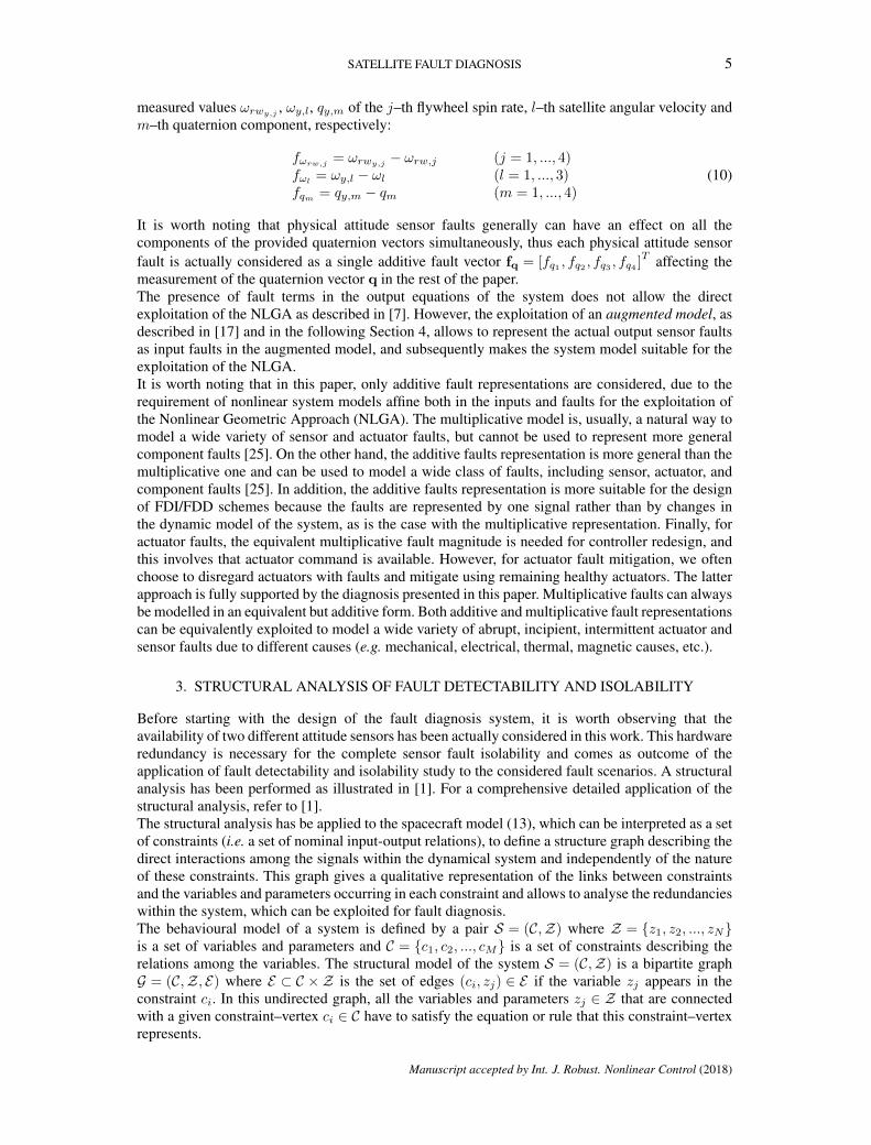
3. STRUCTURAL ANALYSIS OF FAULT DETECTABILITY AND ISOLABILITY
Before starting with the design of the fault diagnosis system, it is worth observing that theavailability of two different attitude sensors has been actually considered in this work. This hardwareredundancy is necessary for the complete sensor fault isolability and comes as outcome of theapplication of fault detectability and isolability study to the considered fault scenarios. A structuralanalysis has been performed as illustrated in [1]. For a comprehensive detailed application of thestructural analysis, refer to [1].The structural analysis has be applied to the spacecraft model (13), which can be interpreted as a setof constraints (i.e. a set of nominal input-output relations), to define a structure graph describing thedirect interactions among the signals within the dynamical system and independently of the natureof these constraints. This graph gives a qualitative representation of the links between constraintsand the variables and parameters occurring in each constraint and allows to analyse the redundancieswithin the system, which can be exploited for fault diagnosis.The behavioural model of a system is defined by a pair S = (C,Z) where Z = z1, z2, ..., zNis a set of variables and parameters and C = c1, c2, ..., cM is a set of constraints describing therelations among the variables. The structural model of the system S = (C,Z) is a bipartite graphG = (C,Z, E) where E ⊂ C × Z is the set of edges (ci, zj) ∈ E if the variable zj appears in theconstraint ci. In this undirected graph, all the variables and parameters zj ∈ Z that are connectedwith a given constraint–vertex ci ∈ C have to satisfy the equation or rule that this constraint–vertexrepresents.
Manuscript accepted by Int. J. Robust. Nonlinear Control (2018)
6 P. BALDI ET AL.
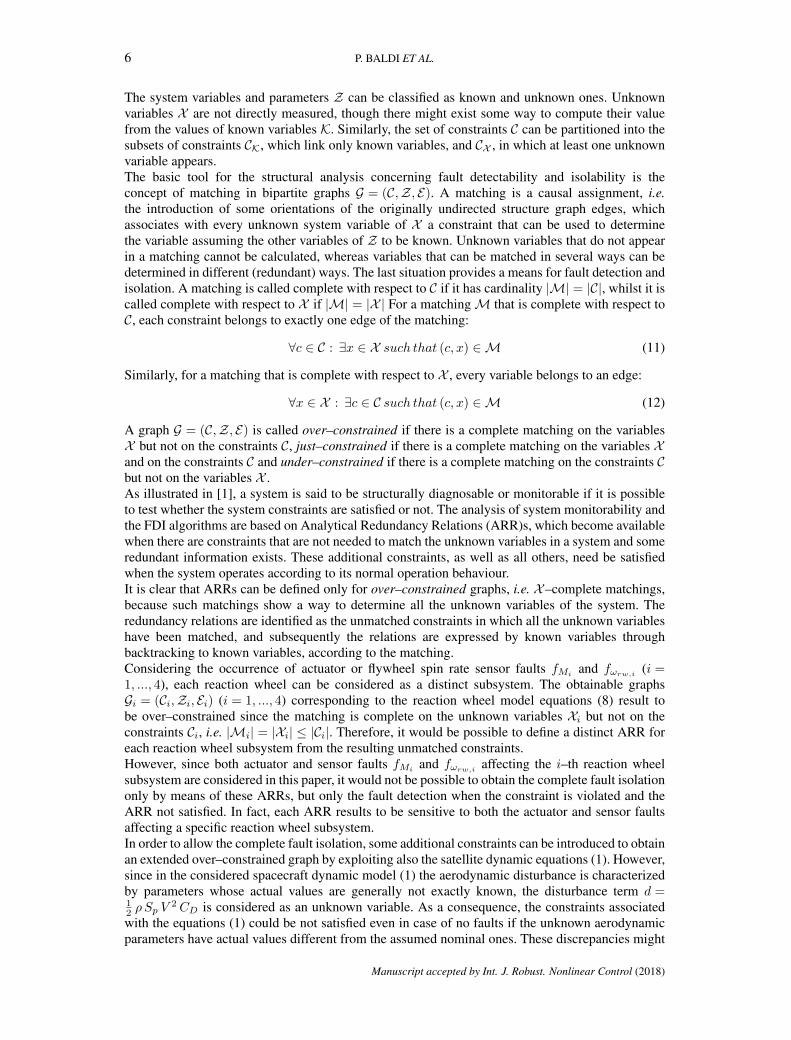
The system variables and parameters Z can be classified as known and unknown ones. Unknownvariables X are not directly measured, though there might exist some way to compute their valuefrom the values of known variables K. Similarly, the set of constraints C can be partitioned into thesubsets of constraints CK, which link only known variables, and CX , in which at least one unknownvariable appears.The basic tool for the structural analysis concerning fault detectability and isolability is theconcept of matching in bipartite graphs G = (C,Z, E). A matching is a causal assignment, i.e.the introduction of some orientations of the originally undirected structure graph edges, whichassociates with every unknown system variable of X a constraint that can be used to determinethe variable assuming the other variables of Z to be known. Unknown variables that do not appearin a matching cannot be calculated, whereas variables that can be matched in several ways can bedetermined in different (redundant) ways. The last situation provides a means for fault detection andisolation. A matching is called complete with respect to C if it has cardinality |M| = |C|, whilst it iscalled complete with respect to X if |M| = |X | For a matchingM that is complete with respect toC, each constraint belongs to exactly one edge of the matching:
∀c ∈ C : ∃x ∈ X such that (c, x) ∈M (11)
Similarly, for a matching that is complete with respect to X , every variable belongs to an edge:
∀x ∈ X : ∃c ∈ C such that (c, x) ∈M (12)
A graph G = (C,Z, E) is called over–constrained if there is a complete matching on the variablesX but not on the constraints C, just–constrained if there is a complete matching on the variables Xand on the constraints C and under–constrained if there is a complete matching on the constraints Cbut not on the variables X .As illustrated in [1], a system is said to be structurally diagnosable or monitorable if it is possibleto test whether the system constraints are satisfied or not. The analysis of system monitorability andthe FDI algorithms are based on Analytical Redundancy Relations (ARR)s, which become availablewhen there are constraints that are not needed to match the unknown variables in a system and someredundant information exists. These additional constraints, as well as all others, need be satisfiedwhen the system operates according to its normal operation behaviour.It is clear that ARRs can be defined only for over–constrained graphs, i.e. X–complete matchings,because such matchings show a way to determine all the unknown variables of the system. Theredundancy relations are identified as the unmatched constraints in which all the unknown variableshave been matched, and subsequently the relations are expressed by known variables throughbacktracking to known variables, according to the matching.Considering the occurrence of actuator or flywheel spin rate sensor faults fMi
and fωrw,i(i =
1, ..., 4), each reaction wheel can be considered as a distinct subsystem. The obtainable graphsGi = (Ci,Zi, Ei) (i = 1, ..., 4) corresponding to the reaction wheel model equations (8) result tobe over–constrained since the matching is complete on the unknown variables Xi but not on theconstraints Ci, i.e. |Mi| = |Xi| ≤ |Ci|. Therefore, it would be possible to define a distinct ARR foreach reaction wheel subsystem from the resulting unmatched constraints.However, since both actuator and sensor faults fMi
and fωrw,iaffecting the i–th reaction wheel
subsystem are considered in this paper, it would not be possible to obtain the complete fault isolationonly by means of these ARRs, but only the fault detection when the constraint is violated and theARR not satisfied. In fact, each ARR results to be sensitive to both the actuator and sensor faultsaffecting a specific reaction wheel subsystem.In order to allow the complete fault isolation, some additional constraints can be introduced to obtainan extended over–constrained graph by exploiting also the satellite dynamic equations (1). However,since in the considered spacecraft dynamic model (1) the aerodynamic disturbance is characterizedby parameters whose actual values are generally not exactly known, the disturbance term d =12 ρSp V
2 CD is considered as an unknown variable. As a consequence, the constraints associatedwith the equations (1) could be not satisfied even in case of no faults if the unknown aerodynamicparameters have actual values different from the assumed nominal ones. These discrepancies might
Manuscript accepted by Int. J. Robust. Nonlinear Control (2018)

SATELLITE FAULT DIAGNOSIS 7
lead to false alarms in the fault detection procedure. Therefore, the ARRs determined on the basisof these constraints would be not robust to aerodynamic parameter uncertainties.As it will be shown in Section 5.4, the exploitation of the NLGA allows to define an additional math-ematical variable xadd, whose dynamic equation xadd = f(ω1, ω2, ω3,q, ωrw,1, ωrw,2, ωrw,3, ωrw,4)is exactly decoupled from the aerodynamic disturbance and any actuator fault fMi
(i = 1, ..., 4),and generally sensitive to all the sensor faults, including any sensor fault fωrw,i
(i = 1, ..., 4). yaddrepresents the corresponding output variable. The constraints associated with this new variableand its dynamic and output equations allow to determine an additional ARR that is robust to theaerodynamic parameter uncertainties and exploitable for the complete isolation of faults fMi orfωrw,i
(i = 1, ..., 4) affecting any reaction wheel subsystem. Since the NLGA variable xadd actuallyis not sensitive to any actuator fault and sensitive to any flywheel spin rate sensor fault, only theoccurrence of any actual fault fωrw,i
(i = 1, ..., 4) results in a violation of the constraints linkedto xadd. The new graph is still over–constrained. Therefore, it would be possible to define fivestructured ARRs from the resulting unmatched constraints, which allow the complete detection andisolation of any actuator or flywheel spin rate sensor fault, without the risk of false alarms due tothe aerodynamic parameter uncertainties.On the other hand, considering the occurrence of satellite attitude and angular velocity sensor faultsfωl
(l = 1, ..., 3) and fq and the presence of a single attitude sensor, the kinematic equations (2) of thesatellite attitude can be considered in the structural analysis. In this case, the corresponding graphG = (C,Z, E) results to be again over–constrained since the matching is complete on the unknownvariables X but not on the constraints C, i.e. |M| = |X | ≤ |C|. Therefore, it would be possible todefine an ARR from the resulting unmatched constraint.However, since the occurrence of both satellite attitude and angular velocity sensor faults fωl
(l = 1, ..., 3) and fq is now considered, it would not be possible to obtain the fault isolation onlyby means of a single ARR, but only the fault detection when the constraint is violated and theARR is not satisfied. In fact, this ARR results to be sensitive to all the satellite attitude and angularvelocity sensor faults fωl
(l = 1, ..., 3) and fq.In order to allow the complete fault isolation, some additional constraints need again to beintroduced. In this case, the equations describing the behaviour of the reaction wheel subsystemscan not be exploited since they are functions only of the satellite attitude and angular velocities,and thus they are not sensitive to any fault affecting the satellite attitude or angular velocity sensors.Moreover, the NLGA variable xadd previously introduced for the detection and isolation of actuatorand flywheel spin rate sensor faults can not be effectively exploited since it leads to an additionalARR that is actually not satisfied when any sensor fault occurs. Hence, another way to determineadditional ARRs to be exploited for the fault isolation task is necessary.In order to determine structured ARRs exploitable for the complete isolation of attitude and angularvelocity sensor faults, a two–steps procedure can be used. Firstly, the NLGA can be exploitedto determine nine new mathematical variables xadd,i (i = 1, ..., 9), whose each dynamic equationxadd,i = f(ω,q) (i = 1, ..., 9) actually results to be decoupled from a specific angular velocitysensor fault fωl
(l = 1, ..., 3) and sensitive to the couple of remaining angular velocity sensor faultsand to the attitude sensor fault fq. yadd,i represent the corresponding output variables. Further detailsabout these NLGA variables are given in Section 5.5. The constraints associated with these newvariables and their dynamic and output equations allow to determine ARRs that are structured withrespect to the angular velocity sensor faults fωl
(l = 1, ..., 3), thought they are still all sensitive to theattitude sensor fault fq. Hence, in case of any angular velocity sensor fault, only a subset of ARRsis not satisfied, thus allowing to recognize the occurred angular velocity sensor fault. However,an additional ARR is still required in order to recognize if an attitude sensor fault or any angularvelocity sensor fault actually occurred, and thus obtain the complete fault isolation.Actually, the only practical way to determine this last ARR consists in the exploitation of somehardware sensor redundancy, which leads to the introduction of additional constraints on theunknown variables. In this paper, the presence of a redundant attitude sensor is then considered. Theattitude measurements of these redundant sensors are represented in the following by means of twodifferent quaternion vectors qy,k (k = 1, 2), which are calculated on the basis of the information
Manuscript accepted by Int. J. Robust. Nonlinear Control (2018)

8 P. BALDI ET AL.
provided by two physical attitude sensors (e.g. star trackers). As a consequence, these attitudemeasurements can be affected by the corresponding sensor faults fq,k (k = 1, 2).Again, the corresponding graph G = (C,Z, E) results to be over–constrained since the matching iscomplete on the unknown variables X but not on the constraints C, i.e. |M| = |X | ≤ |C|. Therefore,exploiting both the NLGA and an additional hardware attitude sensor redundancy, it is possibleto define a sufficient number of ARRs from the resulting unmatched constraints, which allow thedetection and complete isolation of any possible attitude sensor fault fq,k (k = 1, 2) affecting one ofthe two redundant sensors or any angular velocity sensor fault fωl
(l = 1, ..., 3).
4. AUGMENTED NONLINEAR MODEL
The overall nonlinear spacecraft model can be briefly written in the following form:x = n(x) + g(x)u+ `a(x) fa + p(x) dy = h(x) + `s(x) fs
(13)
in which the state vector is x(t) ∈ X (an open subset ofRn), u(t) ∈ Rm is the nominal control inputvector, fa(t) ∈ Rh and fs(t) ∈ Rq are the actuator and sensor fault vectors, respectively, whilstd(t) ∈ Rr is the disturbance vector, and y ∈ Rp is the output vector. n(x), the columns of `a(x),`s(x), g(x) and p(x) are smooth vector fields, and h(x) is a smooth map. In particular, for thecomplete spacecraft model, embedding also the reaction wheel models, the following vectors aredefined:
x = [ω1, ω2, ω3, q, ωrw,1, ωrw,2, ωrw,3, ωrw,4]T
u = [Mc,1, Mc,2, Mc,3, Mc,4]T
d = Faero = 12 ρSp V
2 CDfa = [fM 1, fM 2, fM 3, fM 4]
T
fs =[fω1
, fω2, fω3
, fq,1, fq,2, fωrw,1, fωrw,2
, fωrw,3, fωrw,4
]Ty = [ωy,1, ωy,2, ωy,3, qy,1, qy,2, ωrw,1, ωrw,2, ωrw,3, ωrw,4]
T
(14)
with all the state variables assumed to be measurable,
h(x) = `s(x) =
I3 0 00 I4 00 I4 00 0 I4
(15)
due to the considered attitude sensor redundancy and the terms n(x), g(x), `a(x) and p(x) derivedfrom the equations of (1), (2) and (8).Considering the approach proposed in [17] for the diagnosis of sensor faults, the spacecraft modelcan be augmented by adding new state variables z =
∫ t0y(τ)dτ corresponding to the integrated
output variables, so that z(t) = h(x) + `s(x)fs. The augmented system model with the new statevariables z and the corresponding new output variables w is therefore given as x = n(x) + g(x)u+ `a(x) fa + p(x) d
z = h(x) + `s(x) fsw = z
(16)
or more synthetically as ˙x = f(x) + g(x)u+ ¯(x) f + p(x) dy = w = h(x)
(17)
where, for the considered spacecraft model, it results
x =[xT , zT
]Tz =
[zω1
, zω2, zω3
, zq1 , zq2 , zωrw,1, zωrw,2
, zωrw,3, zωrw,4
]Tf =
[faT , fs
T]T (18)
Manuscript accepted by Int. J. Robust. Nonlinear Control (2018)

SATELLITE FAULT DIAGNOSIS 9
f(x) =
[n(x)h(x)
], g(x) =
[g(x)
0
], h(x) =
[0 I15
](19)
¯(x) =
`a(x) 0
0 `s(x)
, p(x) =
[p(x)
0
](20)
where zωl(l = 1, ..., 3), the vectors zqk
(k = 1, 2), zωrw,j (j = 1, ..., 4) correspond to the integratedoutput variables
∫ t0ωy,l(τ)dτ ,
∫ t0
qy,k(τ)dτ ,∫ t
0ωrwy,j
(τ)dτ of the l–th satellite angular velocitymeasurement, k–th quaternion vector measurement and j–th flywheel spin rate measurement,respectively. It can be seen that the augmented model (17) of the spacecraft now results to be affinein all the control inputs and both actuator and sensor fault inputs. Thus, the NLGA can be exploitedto design aerodynamic and fault decoupled adaptive observers also for the sensor fault diagnosis, asdescribed in Section 5.
5. FAULT DIAGNOSIS
5.1. Nonlinear Geometric Approach
The NonLinear Geometric Approach was formally developed in [7], and it relies on a coordinatechange in the state and output spaces providing an observable subsystem which, if it exists, isaffected by the fault, but unaffected by disturbances and the other faults to be decoupled. TheNLGA estimation filters for FDD are designed by exploiting the properties of this subsystem. For acomprehensive detailed application of the NLGA, refer to [7].In particular, the approach consider a generic nonlinear system model in the form
x = n(x) + g(x)u+ `(x) f + p(x) dy = h(x)
(21)
in which the state vector x ∈ X (an open subset of R`n), u(t) ∈ R`u is the nominal control inputvector, f(t) ∈ R is the fault, d(t) ∈ R`d the disturbance vector (including also the faults to bedecoupled), and y ∈ R`m the output vector. n(x), `(x), the columns of g(x) and p(x) are smoothvector fields, and h(x) is a smooth map. Therefore, if P represents the distribution spanned by thecolumn of p(x), the NLGA method can be devised as follows [7]:
1. determine the minimal conditioned invariant distribution containing P (denoted with∑
P∗ );
2. by using (∑
P∗ )⊥ (i.e. the maximal conditioned invariant codistribution contained in P⊥),
determine the largest observability codistribution contained in P⊥ (denoted with Ω∗);3. if `(x) /∈ (Ω∗)
⊥, the design procedure can continue, otherwise the fault is not detectable;4. whenever the previous condition is satisfied, it can be found a surjection Ψ1 and a function
Φ1 fulfilling Ω∗ ∩ spandh = spand(Ψ1 h) and Ω∗ = spand(Φ1), respectively.
The functions Ψ(y) and Φ(x) defined as
Ψ(y) =
(y1
y2
)=
(Ψ1(y)H2y
),Φ(x) =
x1
x2
x3
=
Φ1(x)H2h(x)Φ3(x)
(22)
are (local) diffeomorphisms, where H2 is a selection matrix (i.e. a matrix in which any row has all0 entries but one, which is equal to 1). x1 = Φ1(x) represents the measured part of the state whichis affected by f and not affected by d, whilst x2 and x3 represent the measured and not measuredpart of the state, which are affected by f and d. In many cases x3 it is not present. In the new (local)
Manuscript accepted by Int. J. Robust. Nonlinear Control (2018)
10 P. BALDI ET AL.
coordinate defined previously, the system is described by the relations:
˙x1 = n1(x1, x2) + g1(x1, x2)u+ `1(x1, x2, x3) f˙x2 = n2(x1, x2, x3) + g2(x1, x2, x3)u+
+`2(x1, x2, x3) f + p2(x1, x2, x3) d˙x3 = n3(x1, x2, x3) + g3(x1, x2, x3)u+
+`3(x1, x2, x3) f + p3(x1, x2, x3) dy1 = h(x1)y2 = x2
(23)
with `1(x1, x2, x3) 6= 0 not identically zero. Denoting x2 with y2 and considering it as anindependent input, the x1–subsystem, which is affected by the single fault fu and decoupled fromthe disturbance vector d (embedding also the other faults to be decoupled), can be defined as follows:
˙x1 = n1(x1, y2) + g1(x1, y2)u+ `1(x1, y2, x3) fy1 = h(x1)
(24)
with `1(x1, y2, x3) 6= 0 not identically zero. This subsystem is exploited for the design of theadaptive observers and residual filters for fault diagnosis purpose.
5.2. Generic Adaptive Input Fault Estimation Filter
An adaptive observer can be designed for state observation and estimation of generic faults on thebasis of the work presented in [17]. Consider a generic nonlinear system described by
˙x(t) = Ax(t) + W f(x(t), t) + Bu(t) + Dfa(t)y(t) = Cx(t)
(25)
where x ∈ Rn, u ∈ Rm and y ∈ Rp denotes, respectively, the vector of state variables, inputs andoutputs, fa ∈ Rq is a not measurable vector which is considered as an additive term resultingfrom generic input faults. The nonlinear continuous term f(x(t), t) ∈ Rj is assumed to be known.A ∈ Rn×n, B ∈ Rn×m, C ∈ Rp×n, D ∈ Rp×q (p ≥ q), and W ∈ Rn×j are known constant matriceswith C and D being of full rank. The following assumptions are made:
Assumption 1. For every complex number s with nonnegative real part,
rank
[sIn − A
C
]= n (26)
Assumption 2. The nonlinear term f(x(t), t) is assumed to be known and Lipschitz about xuniformly, i.e. ∀x, ˆx ∈ Rn, ∥∥f(x(t), t)− f(ˆx(t), t)
∥∥ ≤ Lf ∥∥x(t)− ˆx(t)∥∥ (27)
where Lf is the Lipschitz constant and assumed to be unknown.
Assumption 3. The fault vector fa and its derivative fa satisfy the following norm boundedconstraints:
‖fa‖ ≤ ρa,∥∥fa∥∥ ≤ ρaa (28)
where ρa and ρaa are known positive constants.
Lemma 1. The pair (A, C) is observable if Assumption 1 holds.
This Lemma is directly derived from the Popov-Belevitch-Hautus (PBH) observability criterion.It follows from Lemma 1 that there exists a matrix L ∈ Rn×p such that A− LC is stable, and thusfor any Q > 0, the Lyapunov equation
(A− LC)TP + P (A− LC) = −Q (29)
has a unique solution P = PT > 0, where P ∈ Rn×n is a symmetric positive definite matrix andQ ∈ Rn×n.
Manuscript accepted by Int. J. Robust. Nonlinear Control (2018)
SATELLITE FAULT DIAGNOSIS 11
Remark 1. It follows from Assumption 1 that the pair (A, C) is observable, which provides thenecessary and sufficient condition for the existence of an observer for system (25). Assumption 2states that the considered nonlinear system is Lipschitz. Many practical systems satisfy the Lipschitzcondition, at least locally. In Assumption 2 the generic input fault fa is assumed to be nonzero anddifferentiable after its occurrence. This assumption is quite general either for constant faults andtime–varying faults at limited rates.
Assumption 4. There exists an arbitrary matrix F ∈ Rh×p such that
DTP = FC (30)
For system (25) an adaptive observer is proposed in the following form:˙x(t) = Aˆx(t) + W f(ˆx, t) + Bu(t) + L(y − ˆy) + 1
2 kWH(y − ˆy) + Dfaˆy = C ˆx
(31)
where the observer gain L ∈ Rn×p, H ∈ Rj×p is a matrix to be determined and k satisfies thefollowing adaptation law:
˙k = lk
∥∥H(y − ˆy)∥∥2
(32)
where lk is a positive constant.The term fa represents the estimated fault and its dynamics is defined as:
˙fa = ΓF (y − ˆy)− εΓfa (33)
where Γ ∈ Rh×h is a symmetric positive definite matrix representing the learning rate, F ∈ Rh×p isa matrix to be determined and ε is a positive scalar.Denote ex = x− ˆx, ey = y − ˆy and ef = fa − fa. Then, after the occurrence of the fault, thedynamics of the state estimation error is obtained from
ex = (A− LC)ex + W (f(x, t)− f(ˆx, t)) + Def (34)
The following regions can be defined:
Ω1 =
(ey, fa)|λmin(P )
‖C‖2 ‖ey‖2
+ λmin(Γ−1)2
∥∥∥fa∥∥∥2
≤ λmin(Γ−1)ρ2a + µ3
µ6
Ω2 =
(ey, fa)|λmin(P )
‖C‖2 ‖ey‖2
+ λmin(Γ−1)2
∥∥∥fa∥∥∥2
> λmin(Γ−1)ρ2a + µ3
µ6
µ1 = λmin(−(A− LC)TP − P (A− LC)− 2In) > 0µ2 = λmin(εI −G) > 0µ3 = ρ2
aaλmax(Γ−1G−1Γ−1) + ερ2a
µ4 = min(µ1, µ2)µ5 = max(λmax(P ), λmax(Γ−1))µ6 = µ4/µ5
(35)
where G ∈ Rq×q, P = PT ∈ Rn×n are symmetric positive definite matrices and λmin and λmax arethe smallest and largest eigenvalues, respectively.
Theorem 1. Given system (25) with Assumptions 1, 2 and 3, if there exist matrices L, F , H andP = PT > 0 such that
DTP = FC (36)
WTP = HC (37)
−Q+ 2In < 0 (38)
where −Q = (A− LC)TP + P (A− LC) ∈ Rn×n, then for a given matrix Γ and a positive scalarε, the error dynamics (34) is uniformly bounded and (ey, fa) converges to Ω1 at a rate greater thane−µ6t [17].
Manuscript accepted by Int. J. Robust. Nonlinear Control (2018)
12 P. BALDI ET AL.
ProofConsider the Lyapunov function as
V = eTxPex + l−1k e2
k/2 + eTf Γ−1ef (39)
where ek = k − k, k is a constant which is defined as k = L2f . The time derivative of V can be
shown to be
V ≤ −eTxQex + ‖ex‖2 + (L2f − k)‖HCex‖2 − ek
∥∥HCex∥∥2+ 2eTf Γ−1fa + 2εeTf fa − 2εeTf ef
≤ eTx (−Q+ 2I)ex + 2eTf Γ−1fa + 2εeTf fa − 2εeTf ef(40)
Since 2XTY ≤ 1αX
TGX + αY TG−1Y holds for any scalar α > 0 and symmetric positive definitematrix G, therefore
2eTf Γ−1fa ≤ eTf Gef + fTa Γ−1G−1Γ−1fa ≤ eTf Gef + ρaaλmax(Γ−1G−1Γ−1) (41)
Moreover2εeTf fa ≤ ε‖ef‖
2+ ερ2
a (42)
Substituting (41) and (42) in (40) gives
V ≤ −eTx (Q− 2I)ex + eTf (G− εI)ef + ρaaλmax(Γ−1G−1Γ−1) + ερ2a
≤ −µ1‖ex‖2 − µ2‖ef‖2 + µ3
≤ −µ4(‖ex‖2 + ‖ef‖2) + µ3
(43)
Moreover, from (39)
V ≤ λmax(P )‖ex‖2 + λmax(Γ−1)‖ef‖2
≤ max(λmax(P ), λmax(Γ−1))(‖ex‖2 + ‖ef‖2)
= µ5(‖ex‖2 + ‖ef‖2)
(44)
ThenV ≤ −µ6V + µ3 (45)
For any real constant p and q ∈ R, it results that
(p− q)2 ≥ p2
2− q2 (46)
Therefore
V ≥ λmin(P )‖ex‖2 + λmin(Γ−1)‖ef‖2 ≥λmin(P )
‖C‖2‖ey‖2 + λmin(Γ−1)
∥∥∥fa∥∥∥2
2− ρ2
a
(47)
If (ey, fa) ∈ Ω2, then V > µ3/µ6 and consequently V < 0. Therefore, it can be concluded that(ey, fa) is uniformly bounded and converges to Ω1 exponentially at a rate greater than e−µ6t.
Remark 2. The problem of finding matrices P = PT , L, H and F to simultaneously satisfy theinequality (38) and equalities (36) and (37) can be transformed into the following LMI optimizationproblem:
minimize γ1 + γ2 subject to P > 0 and
PA+ ATP − Y C − CTY T + 2In < 0[γ1Iq DTP − FC
(DTP − FC)T
γ1In
]> 0,
[γ2Ij WTP −HC
(WTP −HC)T
γ2In
]> 0
(48)
where Y = PL.
Manuscript accepted by Int. J. Robust. Nonlinear Control (2018)
SATELLITE FAULT DIAGNOSIS 13
5.3. Adaptation of the Generic Adaptive Estimator Filter in case of Output Sensor Faults
In a similar way, an adaptive observer can be designed for state observation and estimation ofgeneric sensor faults on the basis of the work presented in [17]. Consider a generic nonlinear systemdescribed by
x(t) = Ax(t) +Wf(x, t) +Bu(t)y(t) = Cx(t) +Dfs(t)
(49)
where x ∈ Rn, u ∈ Rm and y ∈ Rp denotes, respectively, the vector of state variables, inputs andoutputs, fs ∈ Rq is a not measurable vector which is considered as an additive term resultingfrom output sensor faults. The nonlinear continuous term f(x, t) ∈ Rj is assumed to be known.A ∈ Rn×n,B ∈ Rn×m,C ∈ Rp×n,D ∈ Rp×q (p ≥ q), andW ∈ Rn×j are known constant matriceswith D being of full column rank. The following assumptions are made:
Assumption 5. The nonlinear term f(x, t) is assumed to be known and Lipschitz about x uniformly,i.e. ∀x, x ∈ Rn,
‖f(x(t), t)− f(x(t), t)‖ ≤ Lf ‖x(t)− x(t)‖ (50)
where Lf is the Lipschitz constant and assumed to be unknown.
Assumption 6. The output sensor fault vector fs and its derivative fs satisfy the following normbounded constraints:
‖fs‖ ≤ ρs,∥∥fs∥∥ ≤ ρss (51)
where ρs and ρss are known positive constants.
As described in [17], for system (49) a new state variable z =∫ t
0y(τ)dτ can be defined so that
z(t) = Cx(t) +Dfo(t). An augmented system with the new state z and output w is therefore givenas x(t) = Ax(t) +Wf(x, t) +Bu(t)
z(t) = Cx(t) +Dfo(t)w(t) = z(t)
(52)
or in matricial form as[xz
]=
[A 0C 0
] [xz
]+
[Wf(x, t)
0
]+
[B0
]u+
[0D
]fs (53)
This system can further be rewritten in a more compact form as˙x(t) = Ax(t) + Wf(x, t) + Bu(t) + Dfo(t)y(t) = w(t) = Cx(t)
(54)
where x ∈ Rn+p, y = w ∈ Rp, A =
[A 0C 0
]∈ R(n+p)×(n+p), B =
[B0
]∈ R(n+p)×m, D =[
0D
]∈ R(n+p)×q, C =
[0 Ip
]∈ Rp×(n+p), W =
[W0
]∈ R(n+p)×m. It can be noted that
the original sensor fault affecting the system output is now modelled as an input fault in theaugmented system 54. Therefore, the same filter design procedure described in Section 5.2 forgeneric input faults fu can be adapted and exploited in order to design an adaptive filter for theestimation of a generic output sensor fault fo, where n = n+ p, p = p, m = m, q = q and j = j.
5.4. Design of Adaptive Filters for the Estimation of Reaction Wheel Actuator Faults and FlywheelSpin Rate Sensor Faults
The NLGA FDD system is designed on the basis of a input affine nonlinear model structure (21)as described in [7]. With the assumption of a single actuator or sensor fault occurring at any time,it is possible to design distinct adaptive observers, which are specifically designed to accuratelyestimate a particular actuator or sensor fault. The provided fault estimates can be directly exploited
Manuscript accepted by Int. J. Robust. Nonlinear Control (2018)
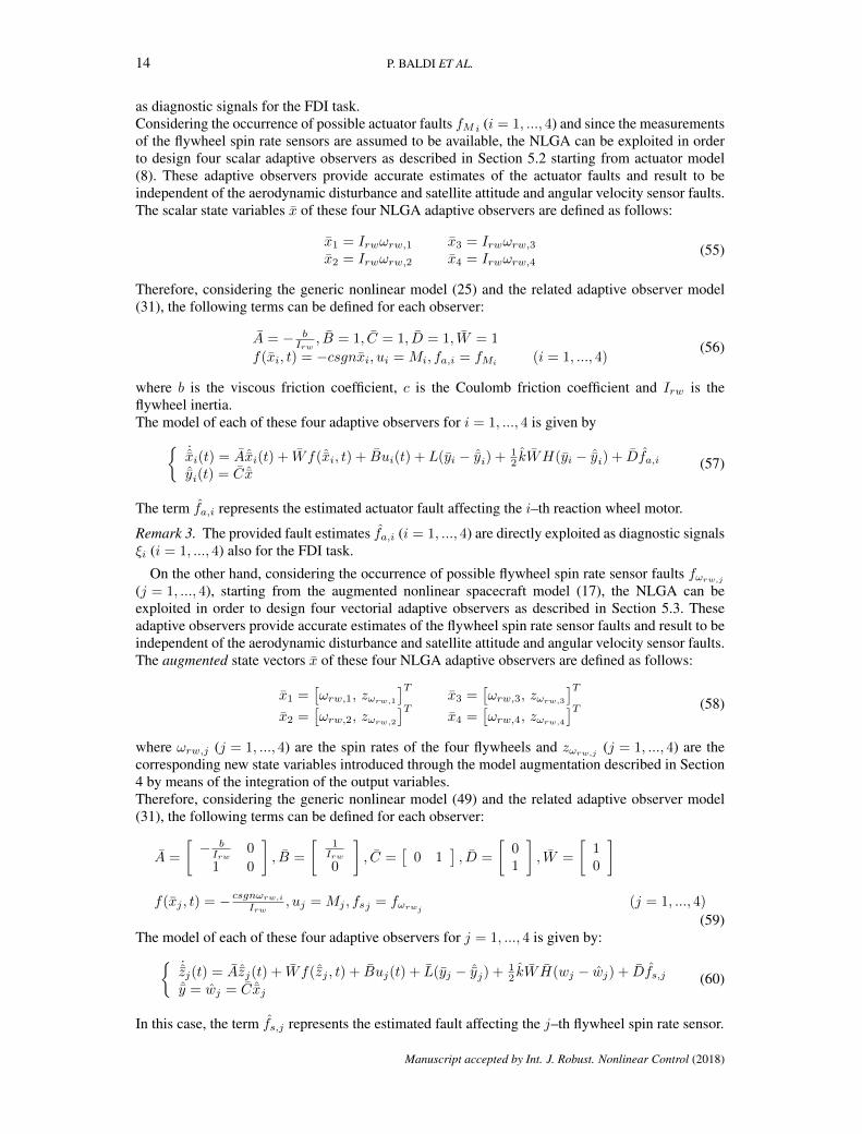
14 P. BALDI ET AL.
as diagnostic signals for the FDI task.Considering the occurrence of possible actuator faults fMi (i = 1, ..., 4) and since the measurementsof the flywheel spin rate sensors are assumed to be available, the NLGA can be exploited in orderto design four scalar adaptive observers as described in Section 5.2 starting from actuator model(8). These adaptive observers provide accurate estimates of the actuator faults and result to beindependent of the aerodynamic disturbance and satellite attitude and angular velocity sensor faults.The scalar state variables x of these four NLGA adaptive observers are defined as follows:
x1 = Irwωrw,1 x3 = Irwωrw,3x2 = Irwωrw,2 x4 = Irwωrw,4
(55)
Therefore, considering the generic nonlinear model (25) and the related adaptive observer model(31), the following terms can be defined for each observer:
A = − bIrw
, B = 1, C = 1, D = 1, W = 1
f(xi, t) = −csgnxi, ui = Mi, fa,i = fMi(i = 1, ..., 4)
(56)
where b is the viscous friction coefficient, c is the Coulomb friction coefficient and Irw is theflywheel inertia.The model of each of these four adaptive observers for i = 1, ..., 4 is given by
˙xi(t) = Aˆxi(t) + Wf(ˆxi, t) + Bui(t) + L(yi − ˆyi) + 12 kWH(yi − ˆyi) + Dfa,i
ˆyi(t) = C ˆx(57)
The term fa,i represents the estimated actuator fault affecting the i–th reaction wheel motor.
Remark 3. The provided fault estimates fa,i (i = 1, ..., 4) are directly exploited as diagnostic signalsξi (i = 1, ..., 4) also for the FDI task.
On the other hand, considering the occurrence of possible flywheel spin rate sensor faults fωrw,j
(j = 1, ..., 4), starting from the augmented nonlinear spacecraft model (17), the NLGA can beexploited in order to design four vectorial adaptive observers as described in Section 5.3. Theseadaptive observers provide accurate estimates of the flywheel spin rate sensor faults and result to beindependent of the aerodynamic disturbance and satellite attitude and angular velocity sensor faults.The augmented state vectors x of these four NLGA adaptive observers are defined as follows:
x1 =[ωrw,1, zωrw,1
]Tx3 =
[ωrw,3, zωrw,3
]Tx2 =
[ωrw,2, zωrw,2
]Tx4 =
[ωrw,4, zωrw,4
]T (58)
where ωrw,j (j = 1, ..., 4) are the spin rates of the four flywheels and zωrw,j(j = 1, ..., 4) are the
corresponding new state variables introduced through the model augmentation described in Section4 by means of the integration of the output variables.Therefore, considering the generic nonlinear model (49) and the related adaptive observer model(31), the following terms can be defined for each observer:
A =
[− bIrw
0
1 0
], B =
[1Irw0
], C =
[0 1
], D =
[01
], W =
[10
]f(xj , t) = − csgnωrw,i
Irw, uj = Mj , fsj = fωrwj
(j = 1, ..., 4)
(59)The model of each of these four adaptive observers for j = 1, ..., 4 is given by:
˙zj(t) = Aˆzj(t) + Wf(ˆzj , t) + Buj(t) + L(yj − ˆyj) + 12 kW H(wj − wj) + Dfs,j
ˆy = wj = C ˆxj(60)
In this case, the term fs,j represents the estimated fault affecting the j–th flywheel spin rate sensor.
Manuscript accepted by Int. J. Robust. Nonlinear Control (2018)

SATELLITE FAULT DIAGNOSIS 15
Remark 4. The provided fault estimates fs,j (j = 1, ..., 4) are directly exploited as diagnostic signalsξi (i = 5, ..., 8) for the FDI task.
Remark 5. It is worth noting that, actually, each of the eight NLGA adaptive observers describedabove results to be sensitive to the couple of faults fMi
, fωrw,j(i = j), i.e. the actuator and flywheel
spin rate sensor faults related to the same i–th reaction wheel, respectively.
In fact, the flywheel spin rate sensor fault fωrw,jdirectly affects the residual signal yi −ˆyi driving
the actuator fault estimate of the adaptive filters relying on the variables (55). On the other hand,the actuator fault fMi
still indirectly affects, through the integration of the measured sensor outputs,the residual signal yj −ˆyj driving the sensor fault estimate of the adaptive filters relying on thevariables (58).However, since each of these eight adaptive estimation filters is designed to provide accurateestimates with respect to the occurrence of a specific actuator or flywheel spin rate sensor fault,the provided signals fa,i (i = 1, ..., 4) result to be correct fault estimates only in case of actuatorfaults fMi
, whilst they do not represent estimates of the actual faults in case of flywheel spin ratesensor faults fωrw,j . Analogously, the provided signals fs,j (j = 1, ..., 4) result to be correct faultestimates only in case of sensor faults fωrw,j
, whilst they do not represent estimates of the actualfaults in case of actuator faults fMi
.Therefore, in general, these estimates allow for the isolation of the reaction wheel subsystemaffected by a possible actuator or sensor fault, but it could not be possible to achieve an exact andcomplete fault isolation by exploiting only these signals. This can be achieved, thanks to the NLGA,by designing and exploiting an additional residual filter in order to precisely classify a detected faultas an actuator or sensor fault with the assumption of a single actuator or sensor fault occurring atany time. The use of the NLGA results to be fundamental to design an additional residual filter thatresults to be decoupled from the aerodynamic disturbance in order to obtain a diagnostic signal notsubject to detection errors due to parametric uncertainties of the aerodynamic disturbance model.This NLGA residual filter exploits also satellite attitude and angular speed measurements in additionto the flywheel spin rate measurements. The dynamic equation determined through the NLGAresults to be insensitive to any possible actuator fault and sensitive to a mathematical combinationof all the spacecraft sensor faults, and thus also to the flywheel spin rate sensor faults.Starting from (24), a generic residual generator in filter form is modelled as follows:
ξ = n1(y1, y2) + g1(y1, y2)uc + L(y1 − ξ)ε = y1 − ξ
(61)
where L > 0 is the gain of the asymptotically stable residual filter and ε is the generated diagnosticsignal. The state vector x of this additional residual generator, obtained by means of the NLGA onthe basis of (13), is defined as follows:
x =[rxcp(Ixxω1 + T1Irwωrw) + rycp(Iyyω2 + T2Irwωrw) + rzcp(Izzω3 + T3Irwωrw)
](62)
where T1, T2 and T3 are the rows of the matrix Trw, zωl(l = 1, ..., 3).
Remark 6. The provided residual signal ε is exploited as additional diagnostic signal ξ9 to preciselyclassify a detected fault as an actuator or flywheel spin rate sensor fault for the complete isolation.After the correct isolation of the occurred actuator or sensor fault, the corresponding accurateestimate is selected among the diagnostic signals ξ1, ..., ξ8.
5.5. Design of Adaptive Filters for the Estimation of Satellite Attitude and Angular Velocity SensorFaults
Considering the occurrence of possible faults fq,k (k = 1, 2) affecting the two considered attitudesensors, starting from the augmented nonlinear spacecraft model (17), the NLGA can be exploitedin order to design two adaptive observers as described in Section 5.3. These adaptive observersprovide accurate estimates of the attitude sensor fault vectors and result to be independent of theaerodynamic disturbance and actuator and sensor faults affecting the reaction wheel subsystems.
Manuscript accepted by Int. J. Robust. Nonlinear Control (2018)
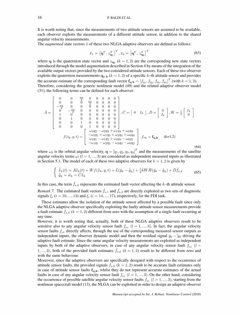
16 P. BALDI ET AL.
It is worth noting that, since the measurements of two attitude sensors are assumed to be available,each observer exploits the measurements of a different attitude sensor, in addition to the sharedangular velocity measurements.The augmented state vectors x of these two NLGA adaptive observers are defined as follows:
x1 =[qT , zTq1
]T, x2 =
[qT , zTq2
]T (63)
where q is the quaternion state vector and zqk(k = 1, 2) are the corresponding new state vectors
introduced through the model augmentation described in Section 4 by means of the integration of theavailable output vectors provided by the two considered attitude sensors. Each of these two observerexploits the quaternion measurements qy,k (k = 1, 2) of a specific k–th attitude sensor and providesthe accurate estimate of the corresponding fault vector fq,k = [fq1 , fq2 , fq3 , fq4 ]
T (with k = 1, 2).Therefore, considering the generic nonlinear model (49) and the related adaptive observer model(31), the following terms can be defined for each observer:
A =
0 0 ω02 0 0 0 0 0
0 0 0 ω02 0 0 0 0
−ω02 0 0 0 0 0 0 0
0 −ω02 0 0 0 0 0 0
1 0 0 0 0 0 0 00 1 0 0 0 0 0 00 0 1 0 0 0 0 00 0 0 1 0 0 0 0
, C =
[0 I4
], D =
[0I4
], W = 1
2
[I40
]
f(zk, y, t) =
ω3q2 − ω2q3 + ω1q4 + ω0q3−ω3q1 + ω1q3 + ω2q4 + ω0q4ω2q1 − ω1q2 + ω3q4 − ω0q1−ω1q1 − ω2q2 − ω3q3 − ω0q2
, fsk = fq,k (k=1,2)
(64)where ω0 is the orbital angular velocity, q = [q1, q2, q3, q4]
T and the measurements of the satelliteangular velocity terms ωl (l = 1, ..., 3) are considered as independent measured inputs as illustratedin Section 5.1. The model of each of these two adaptive observers for k = 1, 2 is given by
˙xk(t) = Aˆxk(t) + Wf(ˆxk, y, t) + L(yk − ˆyk) + 12 kW H(yk − ˆyk) + Dfs,k
ˆyk = wk = C ˆxk(65)
In this case, the term fs,k represents the estimated fault vector affecting the k–th attitude sensor.
Remark 7. The estimated fault vectors fs,1 and fs,2 are directly exploited as two sets of diagnosticsignals ξi (i = 10, ..., 13) and ξi (i = 14, ..., 17), respectively, for the FDI task.
These estimates allow the isolation of the attitude sensor affected by a possible fault since onlythe NLGA adaptive observer specifically exploiting the faulty attitude sensor measurements providea fault estimate fs,k (k = 1, 2) different from zero with the assumption of a single fault occurring atany time.However, it is worth noting that, actually, both of these NLGA adaptive observers result to besensitive also to any angular velocity sensor fault fωl
(l = 1, ..., 3). In fact, the angular velocitysensor faults fωl
directly affects, through the use of the corresponding measured sensor outputs asindependent inputs, the observer dynamic model and then the residual signal yk −ˆyk driving theadaptive fault estimate. Since the same angular velocity measurements are exploited as independentinputs by both of the adaptive observers, in case of any angular velocity sensor fault fωl
(l =
1, ..., 3), both of the provided fault estimates fs,k (k = 1, 2) result to be different from zero andwith the same behaviour.Moreover, since the adaptive observers are specifically designed with respect to the occurrence ofattitude sensor faults, the provided signals fs,k (k = 1, 2) result to be accurate fault estimates onlyin case of attitude sensor faults fq,k, whilst they do not represent accurate estimates of the actualfaults in case of any angular velocity sensor fault fωl
(l = 1, ..., 3). On the other hand, consideringthe occurrence of possible satellite angular velocity sensor faults fωl
(l = 1, ..., 3), starting from thenonlinear spacecraft model (13), the NLGA can be exploited in order to design an adaptive observer
Manuscript accepted by Int. J. Robust. Nonlinear Control (2018)

SATELLITE FAULT DIAGNOSIS 17
as described in Section 5.2. In particular, this adaptive observer provide accurate estimates of theangular velocity faults and results to be independent of the aerodynamic disturbance and actuatorand sensor faults affecting the reaction wheel subsystems.The state vector x of this NLGA adaptive observer is defined as follows:
x =
(q21 − q2
2 − q23 + q2
4)(−q2
1 + q22 − q2
3 + q24)
(−q21 − q2
2 + q23 + q2
4)2(q1q2 + q3q4)2(q1q3 + q2q4)2(q1q4 + q2q3)2(q1q2 − q3q4)2(q1q3 − q2q4)2(q2q3 − q1q4)
(66)
Therefore, considering the generic nonlinear model (25) and the related adaptive observer model(31), the following terms can be defined for this observer:
A =
0 0 0 0 0 0 0 ω0 00 0 0 0 0 0 0 0 00 0 0 0 −ω0 0 0 0 00 0 0 0 0 0 0 0 00 0 ω0 0 0 0 0 0 00 0 0 0 0 0 −ω0 0 00 0 0 0 0 ω0 0 0 0−ω0 0 0 0 0 0 0 0 0
0 0 0 0 0 0 0 0 0
, C = I9, D = I9, W = I9
f(x, y, t) =
−2ω2(q1q3 + q2q4) + 2ω3(q1q2 − q3q4)2ω1(q2q3 − q1q4)− 2ω3(q1q2 + q3q4)−2ω1(q1q4 + q2q3) + 2ω2(q1q3 − q2q4)
−2ω2(q2q3 − q1q4) + ω3(−q21 + q2
2 − q23 + q2
4)−2ω1(q1q2 − q3q4) + ω2(q2
1 − q22 − q2
3 + q24)
ω1(−q21 − q2
2 + q23 + q2
4)− 2ω3(q1q3 − q2q4)2ω1(q1q3 + q2q4)− ω3(q2
1 − q22 − q2
3 + q24)
2ω3(q1q4 + q2q3)− ω2(−q21 − q2
2 + q23 + q2
4)2ω2(q1q2 + q3q4)− ω1(−q2
1 + q22 − q2
3 + q24)
fa =
−2fω2(q1q3 + q2q4) + 2fω3
(q1q2 − q3q4)2fω1
(q2q3 − q1q4)− 2fω3(q1q2 + q3q4)
−2fω1(q1q4 + q2q3) + 2fω2(q1q3 − q2q4)−2fω2(q2q3 − q1q4) + fω3(−q2
1 + q22 − q2
3 + q24)
−2fω1(q1q2 − q3q4) + fω2
(q21 − q2
2 − q23 + q2
4)fω1
(−q21 − q2
2 + q23 + q2
4)− 2fω3(q1q3 − q2q4)
2fω1(q1q3 + q2q4)− fω3
(q21 − q2
2 − q23 + q2
4)2fω3(q1q4 + q2q3)− fω2(−q2
1 − q22 + q2
3 + q24)
2fω2(q1q2 + q3q4)− fω1(−q21 + q2
2 − q23 + q2
4)
(67)
where the elements of the additive fault vector fa that is actually estimated by the adaptive observerare functions of the observer state vector x and actual satellite angular velocity sensor faults fωl
(l = 1, ..., 3). In the same way, considering the satellite angular velocity terms ωl (l = 1, ..., 3)as independent measured inputs as illustrated in Section 5.1, the nonlinear terms of the adaptiveobserver are functions of the observer state vector x and satellite angular velocities ωl (l = 1, ..., 3).Therefore, the model of this adaptive observer is given by:
˙x(t) = Aˆx(t) + Wf(ˆx, y, t) + L(y − ˆy) + Dfaˆy = C ˆx
(68)
Manuscript accepted by Int. J. Robust. Nonlinear Control (2018)
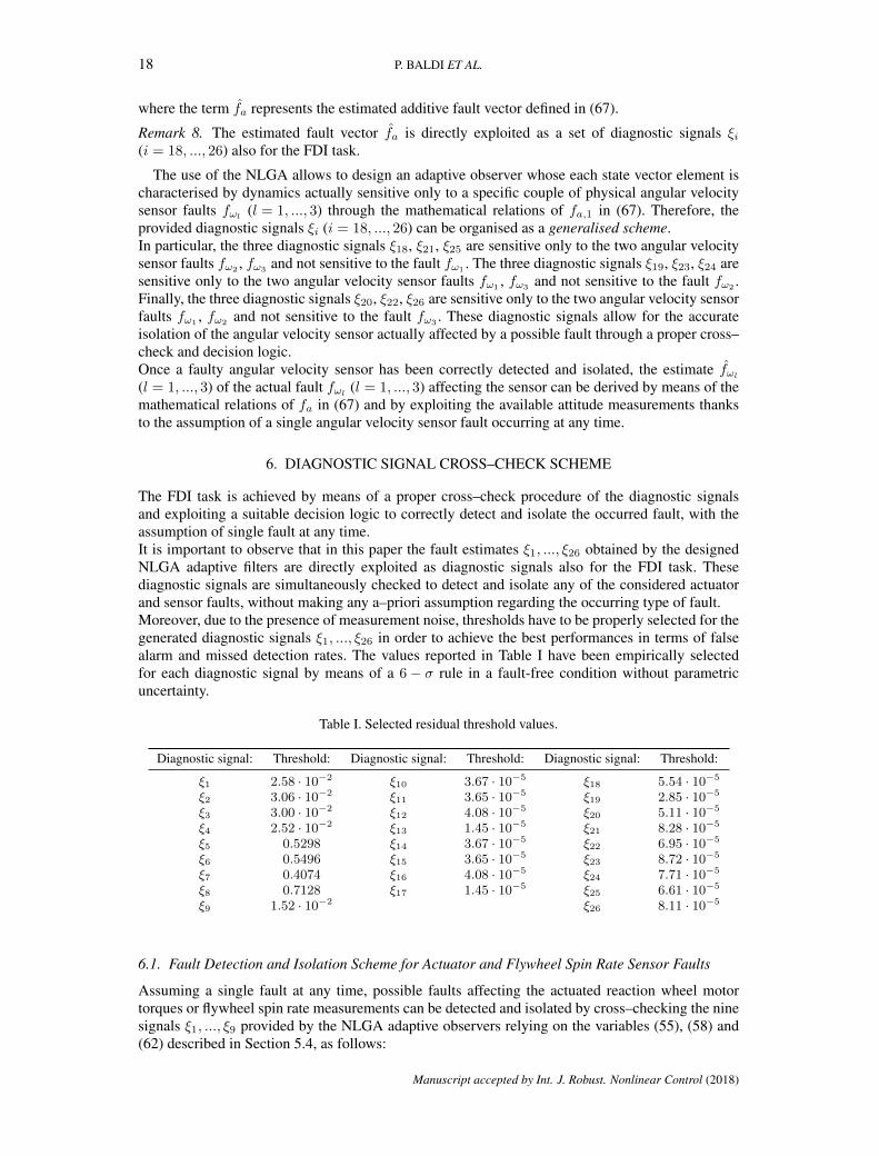
18 P. BALDI ET AL.
where the term fa represents the estimated additive fault vector defined in (67).
Remark 8. The estimated fault vector fa is directly exploited as a set of diagnostic signals ξi(i = 18, ..., 26) also for the FDI task.
The use of the NLGA allows to design an adaptive observer whose each state vector element ischaracterised by dynamics actually sensitive only to a specific couple of physical angular velocitysensor faults fωl
(l = 1, ..., 3) through the mathematical relations of fa,1 in (67). Therefore, theprovided diagnostic signals ξi (i = 18, ..., 26) can be organised as a generalised scheme.In particular, the three diagnostic signals ξ18, ξ21, ξ25 are sensitive only to the two angular velocitysensor faults fω2 , fω3 and not sensitive to the fault fω1 . The three diagnostic signals ξ19, ξ23, ξ24 aresensitive only to the two angular velocity sensor faults fω1 , fω3 and not sensitive to the fault fω2 .Finally, the three diagnostic signals ξ20, ξ22, ξ26 are sensitive only to the two angular velocity sensorfaults fω1
, fω2and not sensitive to the fault fω3
. These diagnostic signals allow for the accurateisolation of the angular velocity sensor actually affected by a possible fault through a proper cross–check and decision logic.Once a faulty angular velocity sensor has been correctly detected and isolated, the estimate fωl
(l = 1, ..., 3) of the actual fault fωl(l = 1, ..., 3) affecting the sensor can be derived by means of the
mathematical relations of fa in (67) and by exploiting the available attitude measurements thanksto the assumption of a single angular velocity sensor fault occurring at any time.
6. DIAGNOSTIC SIGNAL CROSS–CHECK SCHEME
The FDI task is achieved by means of a proper cross–check procedure of the diagnostic signalsand exploiting a suitable decision logic to correctly detect and isolate the occurred fault, with theassumption of single fault at any time.It is important to observe that in this paper the fault estimates ξ1, ..., ξ26 obtained by the designedNLGA adaptive filters are directly exploited as diagnostic signals also for the FDI task. Thesediagnostic signals are simultaneously checked to detect and isolate any of the considered actuatorand sensor faults, without making any a–priori assumption regarding the occurring type of fault.Moreover, due to the presence of measurement noise, thresholds have to be properly selected for thegenerated diagnostic signals ξ1, ..., ξ26 in order to achieve the best performances in terms of falsealarm and missed detection rates. The values reported in Table I have been empirically selectedfor each diagnostic signal by means of a 6− σ rule in a fault-free condition without parametricuncertainty.
Table I. Selected residual threshold values.
Diagnostic signal: Threshold: Diagnostic signal: Threshold: Diagnostic signal: Threshold:
ξ1 2.58 · 10−2 ξ10 3.67 · 10−5 ξ18 5.54 · 10−5
ξ2 3.06 · 10−2 ξ11 3.65 · 10−5 ξ19 2.85 · 10−5
ξ3 3.00 · 10−2 ξ12 4.08 · 10−5 ξ20 5.11 · 10−5
ξ4 2.52 · 10−2 ξ13 1.45 · 10−5 ξ21 8.28 · 10−5
ξ5 0.5298 ξ14 3.67 · 10−5 ξ22 6.95 · 10−5
ξ6 0.5496 ξ15 3.65 · 10−5 ξ23 8.72 · 10−5
ξ7 0.4074 ξ16 4.08 · 10−5 ξ24 7.71 · 10−5
ξ8 0.7128 ξ17 1.45 · 10−5 ξ25 6.61 · 10−5
ξ9 1.52 · 10−2 ξ26 8.11 · 10−5
6.1. Fault Detection and Isolation Scheme for Actuator and Flywheel Spin Rate Sensor Faults
Assuming a single fault at any time, possible faults affecting the actuated reaction wheel motortorques or flywheel spin rate measurements can be detected and isolated by cross–checking the ninesignals ξ1, ..., ξ9 provided by the NLGA adaptive observers relying on the variables (55), (58) and(62) described in Section 5.4, as follows:
Manuscript accepted by Int. J. Robust. Nonlinear Control (2018)
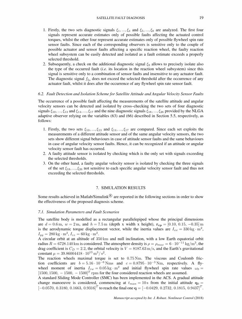
SATELLITE FAULT DIAGNOSIS 19
1. Firstly, the two sets diagnostic signals ξ1, ..., ξ4 and ξ5, ..., ξ8 are analyzed. The first foursignals represent accurate estimates only of possible faults affecting the actuated controltorques, whilst the other four represent accurate estimates only of possible flywheel spin ratesensor faults. Since each of the corresponding observers is sensitive only to the couple ofpossible actuator and sensor faults affecting a specific reaction wheel, the faulty reactionwheel subsystem can be easily detected and isolated as a fault estimate exceeds a properlyselected threshold.
2. Subsequently, a check on the additional diagnostic signal ξ9 allows to precisely isolate alsothe type of the occurred fault (i.e. its location in the reaction wheel subsystem) since thissignal is sensitive only to a combination of sensor faults and insensitive to any actuator fault.The diagnostic signal fξ9 does not exceed the selected threshold after the occurrence of anyactuator fault, whilst it does after the occurrence of any flywheel spin rate sensor fault.
6.2. Fault Detection and Isolation Scheme for Satellite Attitude and Angular Velocity Sensor Faults
The occurrence of a possible fault affecting the measurements of the satellite attitude and angularvelocity sensors can be detected and isolated by cross–checking the two sets of four diagnosticsignals ξ10, ..., ξ13 and ξ14, ..., ξ17 and the nine diagnostic signals ξ18, ..., ξ26 provided by the NLGAadaptive observer relying on the variables (63) and (66) described in Section 5.5, respectively, asfollows:
1. Firstly, the two sets ξ10, ..., ξ13 and ξ14, ..., ξ17 are compared. Since each set exploits themeasurements of a different attitude sensor and of the same angular velocity sensors, the twosets show different signal behaviours in case of attitude sensor faults and the same behavioursin case of angular velocity sensor faults. Hence, it can be recognized if an attitude or angularvelocity sensor fault has occurred.
2. A faulty attitude sensor is isolated by checking which is the only set with signals exceedingthe selected thresholds.
3. On the other hand, a faulty angular velocity sensor is isolated by checking the three signalsof the set ξ18, ..., ξ26 not sensitive to each specific angular velocity sensor fault and thus notexceeding the selected thresholds.
7. SIMULATION RESULTS
Some results achieved in Matlab/Simulink R© are reported in the following sections in order to showthe effectiveness of the proposed diagnosis scheme.
7.1. Simulation Parameters and Fault Scenarios
The satellite body is modelled as a rectangular parallelepiped whose the principal dimensionsare d = 0.6 m, w = 2 m, and h = 7.5 m (depth x width x height), rcp = [0.10, 0.15, −0.35] mis the aerodynamic torque displacement vector, while the inertia values are Ixx = 330 kg ·m2,Iyy = 280 kg ·m2, Izz = 60 kg ·m2.A circular orbit at an altitude of 350 km and null inclination, with a low Earth equatorial orbitradiusR = 6728.140 km is considered. The atmosphere density is ρ = ρmax = 6 · 10−11 kg/m3, thedrag coefficient is CD = 2.2, the orbital velocity is V = 8187.63 m/s, and the Earth’s gravitationalconstant µ = 39.86004418 · 1013 m3/ s2.The reaction wheels maximal torque is set to 0.75 Nm. The viscous and Coulomb fric-tion coefficients are b = 5.16 · 10−6 Nms and c = 0.8795 · 10−3 Nm, respectively. A fly-wheel moment of inertia Irw = 0.05 kg ·m2 and initial flywheel spin rate values ω0 =[1500, 1500, − 1500, − 1500]T rpm for the four considered reaction wheels are assumed.A standard Sliding Mode Controller (SMC) has been implemented in the ACS. A gradual attitudechange manoeuvre is considered, commencing at tman = 10 s from the initial attitude q0 =
[−0.0570, 0.3180, 0.1663, 0.9316]T to reach the final one q = [−0.0429, 0.2732, 0.1815, 0.9437]
T .
Manuscript accepted by Int. J. Robust. Nonlinear Control (2018)
20 P. BALDI ET AL.
These quaternion vectors correspond to [φ0, θ0, ψ0, ]T
= [−15, 35, 25]T deg and [φ, θ, ψ, ]
T=
[−12, 30, 25]T deg for the attitude in Euler angles (i.e. roll, pitch and yaw angles), respectively.
Assuming a single fault at any time, four additive fault scenarios commencing at tfault = 20 s areconsidered:
1. Actuator fault: fM2= −aM ωrw2
− bM with aM linearly passing from zero at t = 20 s to0.003 Nms at t = 30 s and bM = 0.05 Nm;
2. Flywheel sensor fault: fωrw,2= −aωrw
with aωrwlinearly passing from zero at t = 20 s to
−0.5235 rad/s = −100 rpm at t = 45 s and then changing from −0.5235 rad/s = −100 rpmat t = 50 s to −0.2618 rad/s = −50 rpm at t = 55 s;
3. Attitude sensor fault: fq,1 additive on the first quaternion measurement, corresponding to aconstant bias of 8.7266 · 10−4 rad = 0.05 deg on the roll angle measurements;
4. Angular velocity sensor fault: fω3= −aω sin(bωt) with aω linearly passing from zero at
t = 20 s to 6.9808 · 10−4 rad/s at t = 40 s and bω = 0.05π rad/s = 0.025 Hz.
It is noted that the proposed diagnosis scheme does not assume any a–priori hypothesis regardingthe fault type and that the diagnosis system takes into account the possible occurrence of faultsaffecting any actuator or sensor of the satellite ADCS. Moreover, the generic additive faults canbe used to represent different fault causes (e.g. mechanical, electrical, thermal, magnetic damagesand malfunctions, parameter variations, etc.), and behaviours (e.g. lock–in–place, failure, loss ofeffectiveness, drift, bias, etc.). Sensor noises are modelled by Gaussian processes with zero mean.Standard deviations equal to 3 arcsec, 3 arcsec/s and 1 rpm are assumed for the attitude measured inEuler angles, satellite angular speed and flywheel spin rate measurements, respectively. A simulationtime of 60 s with a sampling time of 0.025 s is considered.
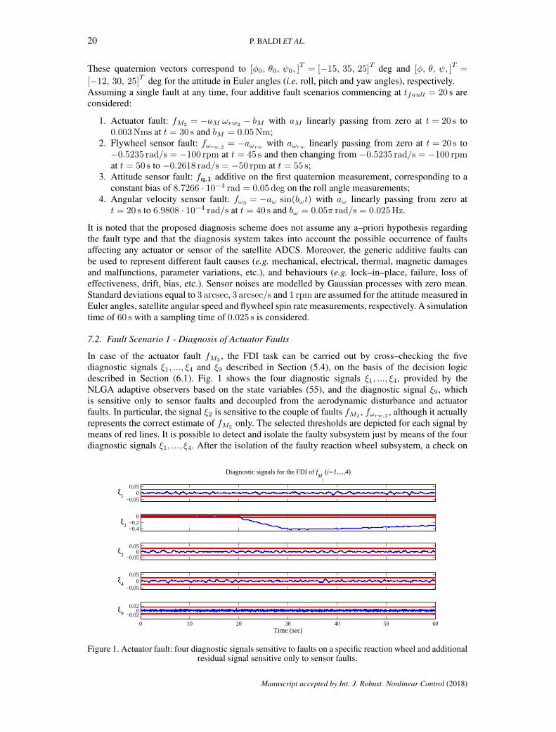
7.2. Fault Scenario 1 - Diagnosis of Actuator Faults
In case of the actuator fault fM2 , the FDI task can be carried out by cross–checking the fivediagnostic signals ξ1, ..., ξ4 and ξ9 described in Section (5.4), on the basis of the decision logicdescribed in Section (6.1). Fig. 1 shows the four diagnostic signals ξ1, ..., ξ4, provided by theNLGA adaptive observers based on the state variables (55), and the diagnostic signal ξ9, whichis sensitive only to sensor faults and decoupled from the aerodynamic disturbance and actuatorfaults. In particular, the signal ξ2 is sensitive to the couple of faults fM2 , fωrw,2 , although it actuallyrepresents the correct estimate of fM2
only. The selected thresholds are depicted for each signal bymeans of red lines. It is possible to detect and isolate the faulty subsystem just by means of the fourdiagnostic signals ξ1, ..., ξ4. After the isolation of the faulty reaction wheel subsystem, a check on
−0.050
0.05ξ
1
Diagnostic signals for the FDI of fM
i
(i=1,...,4)
−0.4−0.2
0ξ
2
−0.050
0.05ξ
3
−0.050
0.05ξ
4
0 10 20 30 40 50 60
−0.020
0.02ξ9
Time (sec)
Figure 1. Actuator fault: four diagnostic signals sensitive to faults on a specific reaction wheel and additionalresidual signal sensitive only to sensor faults.
Manuscript accepted by Int. J. Robust. Nonlinear Control (2018)

SATELLITE FAULT DIAGNOSIS 21
0 10 20 30 40 50 60
−0.4
−0.3
−0.2
−0.1
0
f M2 [N
m]
True and estimated actuator fault fM
2
Time (sec)
Fault Estimate True Fault
Figure 2. Estimate of the actuator fault fM2.
the signal ξ9 allows to precisely isolate also the type of the occurred fault (i.e. its location) since thisresidual is sensitive only to sensor faults and insensitive to actuator faults. It does not exceed theselected threshold in case of actuator faults.Once an actuator fault fMi (i = 1, ..., 4) has been detected and isolated, the corresponding estimateis directly given by the related diagnostic signal fMi
= ξi (i = 1, ..., 4), which has been exploitedalso for the FDI task. Fig. 2 shows the estimate fM2
of the actuator fault fM2provided by the
corresponding NLGA adaptive observer. It can be seen that the adaptive observer provides anaccurate estimate of the occurred fault, even in case of a generic fault function.
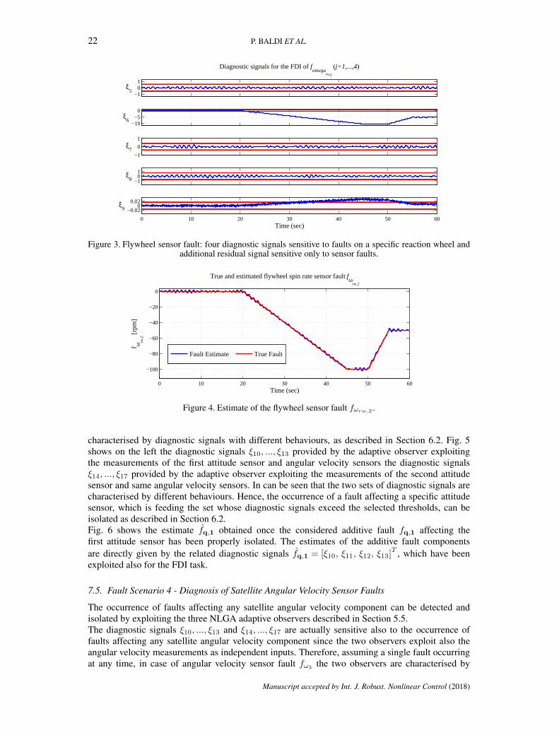
7.3. Fault Scenario 2 - Diagnosis of Flywheel Spin Rate Sensor Faults
On the other hand, in case of the flywheel spin rate sensor fault fωrw,2 , the FDI task can be carriedout by cross–checking the five diagnostic signals ξ5, ..., ξ9 described in Sections (5.4), on the basisof the decision logic described in Section (6.1). Fig. 3 shows the four diagnostic signals ξ5, ..., ξ8provided by the NLGA adaptive observers based on the variables (58). In particular, the signal ξ6 issensitive to the couple of faults fM2 , fωrw,2 , although it actually represents the correct estimate offωrw,2 only. As already described, the diagnostic signal ξ9 is sensitive only to flywheel sensor faultsand decoupled from the aerodynamic disturbance and actuator faults and allows to precisely isolatealso the type (i.e. its location) of the occurred fault since this residual is sensitive only to sensorfaults and insensitive to actuator faults. In this case, it does exceed the selected threshold after thesensor fault occurrence. Hence, the occurred flywheel sensor fault can be correctly isolated thanksto the different behaviour of this additional diagnostic signal. Once a flywheel spin rate sensor faultfωrw,j (j = 1, ..., 4) has been detected and isolated, the corresponding estimate is directly given bythe related diagnostic signal fωrw,j = ξi (i = 6, ..., 9), which has been exploited also for the FDItask. Fig. 4 shows the estimate fωrw,2
of the sensor fault fωrw,2.
Remark 9. It is worth noting that, even if there are detection delays to exceed thresholds, the faultestimates do not suffer from delay since these signals coincide with the diagnostic signals exploitedalso by the FDI system, which are available in real time, and there are no estimation filters to beactivated and initialized after the fault isolation.
7.4. Fault Scenario 3 - Diagnosis of Satellite Attitude Sensor Faults
The occurrence of faults affecting one of the two considered attitude sensors can be detected andisolated by exploiting the first two NLGA adaptive observers described in Section 5.5.The diagnostic signals ξ10, ..., ξ13 and ξ14, ..., ξ17 obtained by means of the corresponding twoadaptive observers represent the correct estimates of the components of possible attitude sensorfaults fq,1 and fq,2 affecting the first and second attitude sensor, respectively. Therefore, assuming asingle fault occurring at any time, in case of attitude sensor fault the two observers, each providingthe estimate of a possible additive fault fq,k (k = 1, 2) affecting a specific attitude sensor, are
Manuscript accepted by Int. J. Robust. Nonlinear Control (2018)
22 P. BALDI ET AL.
−101
ξ5
Diagnostic signals for the FDI of fomega
rw,j
(j=1,...,4)
−10−5
0ξ
6
−1
0
1ξ
7
−101ξ
8
0 10 20 30 40 50 60
−0.020
0.02ξ9
Time (sec)
Figure 3. Flywheel sensor fault: four diagnostic signals sensitive to faults on a specific reaction wheel andadditional residual signal sensitive only to sensor faults.
0 10 20 30 40 50 60
−100
−80
−60
−40
−20
0
f ωrw
,2
[rpm
]
True and estimated flywheel spin rate sensor fault fω
rw,2
Time (sec)
Fault Estimate True Fault
Figure 4. Estimate of the flywheel sensor fault fωrw,2 .
characterised by diagnostic signals with different behaviours, as described in Section 6.2. Fig. 5shows on the left the diagnostic signals ξ10, ..., ξ13 provided by the adaptive observer exploitingthe measurements of the first attitude sensor and angular velocity sensors the diagnostic signalsξ14, ..., ξ17 provided by the adaptive observer exploiting the measurements of the second attitudesensor and same angular velocity sensors. In can be seen that the two sets of diagnostic signals arecharacterised by different behaviours. Hence, the occurrence of a fault affecting a specific attitudesensor, which is feeding the set whose diagnostic signals exceed the selected thresholds, can beisolated as described in Section 6.2.Fig. 6 shows the estimate fq,1 obtained once the considered additive fault fq,1 affecting thefirst attitude sensor has been properly isolated. The estimates of the additive fault componentsare directly given by the related diagnostic signals fq,1 = [ξ10, ξ11, ξ12, ξ13]
T , which have beenexploited also for the FDI task.
7.5. Fault Scenario 4 - Diagnosis of Satellite Angular Velocity Sensor Faults
The occurrence of faults affecting any satellite angular velocity component can be detected andisolated by exploiting the three NLGA adaptive observers described in Section 5.5.The diagnostic signals ξ10, ..., ξ13 and ξ14, ..., ξ17 are actually sensitive also to the occurrence offaults affecting any satellite angular velocity component since the two observers exploit also theangular velocity measurements as independent inputs. Therefore, assuming a single fault occurringat any time, in case of angular velocity sensor fault fω3
the two observers are characterised by
Manuscript accepted by Int. J. Robust. Nonlinear Control (2018)

SATELLITE FAULT DIAGNOSIS 23
0246
x 10−4
ξ10
Diagnostic signals for the FDI of fomega
l
(l=1,...,3) and fq,1
−10−5
05
x 10−5
ξ11
0
10
20
x 10−5
ξ12
0 10 20 30 40 50 60−2
024
x 10−5
ξ13
Time (sec)
−5
0
5x 10
−5
ξ14
Diagnostic signals for the FDI of fomega
l
(l=1,...,3) and fq,2
−5
0
5x 10
−5
ξ15
−5
0
5x 10
−5
ξ16
0 10 20 30 40 50 60−2
0
2x 10
−5
ξ17
Time (sec)
Figure 5. Attitude sensor fault: two sets of diagnostic signals provided by the adaptive observer exploitingthe measurements of the first (left) and second (right) attitude sensor, respectively.
0
5
10x 10
−4
f q 1
True and estimated quaternion fault vector fq,1
−15−10−5
05
x 10−5
f q 2
0123
x 10−4
f q 3
0 10 20 30 40 50 60
02468
x 10−5
f q 4
Time (sec)
Fault Estimate True Fault
Figure 6. Estimate of the additive quaternion fault vector fq,1 associated to the physical attitude sensor fault.
diagnostic signals with the same behaviours and exceeding the selected thresholds, since they exploitthe same angular velocity measurements, as described in Section 6.2. However, it is not yet possibleto isolate the specific faulty angular velocity sensor on the basis of these diagnostic signals only.Therefore, once a fault affecting a generic angular velocity sensor has been detected, the ninediagnostic signals ξ18, ..., ξ26 have to be exploited in order to accurately isolate the specific faultyangular velocity sensor. In particular, Fig. 7 shows the three diagnostic signals ξ18, ξ21, ξ25 thatare sensitive only to the two angular velocity sensor faults fω2
, fω3and not sensitive to the fault
fω1. Fig. 8 shows the three diagnostic signals ξ19, ξ23, ξ24 that are sensitive only to the two angular
velocity sensor faults fω1 , fω3 and not sensitive to the fault fω2 . Finally, Fig. 9 shows the threediagnostic signals ξ20, ξ22, ξ26 that are sensitive only to the two angular velocity sensor faults fω1 ,fω2
and not sensitive to the fault fω3. In this case, in Fig. 9 the last three signals ξ20, ξ22, ξ26 ,
which results to be decoupled from possible faults affecting the third angular velocity sensor, do notexceed the selected thresholds. On the contrary, the other six signals generally result to be sensitiveto the occurred angular velocity sensor fault.Finally, Fig. 10 shows the estimate fω3 obtained once the fault fω3 has been properly isolated. Theestimate of the actual fault is mathematically derived directly from the diagnostic signals ξ18, ..., ξ26,which have been exploited to complete the fault isolation task.
Manuscript accepted by Int. J. Robust. Nonlinear Control (2018)
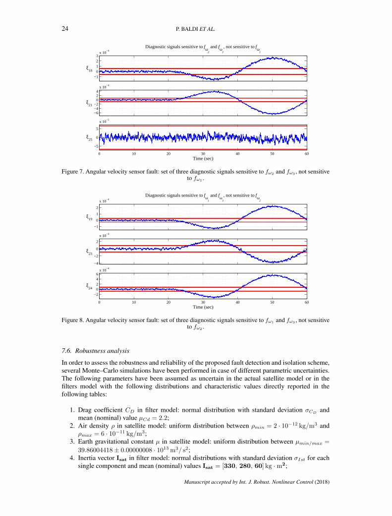
24 P. BALDI ET AL.
−10123
x 10−4
ξ18
Diagnostic signals sensitive to fω
2
and fω
3
, not sensitive to fω
1
−6−4−2
024
x 10−4
ξ21
0 10 20 30 40 50 60
−5
0
5
x 10−5
ξ25
Time (sec)
Figure 7. Angular velocity sensor fault: set of three diagnostic signals sensitive to fω2 and fω3 , not sensitiveto fω1 .
−1
0
1
2
x 10−4
ξ19
Diagnostic signals sensitive to fω
1
and fω
3
, not sensitive to fω
2
−4
−2
0
2
x 10−4
ξ23
0 10 20 30 40 50 60
−20246
x 10−4
ξ24
Time (sec)
Figure 8. Angular velocity sensor fault: set of three diagnostic signals sensitive to fω1 and fω3 , not sensitiveto fω2 .
7.6. Robustness analysis
In order to assess the robustness and reliability of the proposed fault detection and isolation scheme,several Monte–Carlo simulations have been performed in case of different parametric uncertainties.The following parameters have been assumed as uncertain in the actual satellite model or in thefilters model with the following distributions and characteristic values directly reported in thefollowing tables:
1. Drag coefficient CD in filter model: normal distribution with standard deviation σCDand
mean (nominal) value µCd = 2.2;2. Air density ρ in satellite model: uniform distribution between ρmin = 2 · 10−12 kg/m3 andρmax = 6 · 10−11 kg/m3;
3. Earth gravitational constant µ in satellite model: uniform distribution between µmin/max =
39.86004418± 0.00000008 · 1013 m3/ s2;4. Inertia vector Isat in filter model: normal distributions with standard deviation σIst for each
single component and mean (nominal) values Isat = [330, 280, 60] kg ·m2;
Manuscript accepted by Int. J. Robust. Nonlinear Control (2018)

SATELLITE FAULT DIAGNOSIS 25
−5
0
5
x 10−5
ξ20
Diagnostic signals sensitive to fω
1
and fω
2
, not sensitive to fω
3
−1
0
1x 10
−4
ξ22
0 10 20 30 40 50 60
−1
0
1x 10
−4
ξ26
Time (sec)
Figure 9. Angular velocity sensor fault: set of three diagnostic signals sensitive to fω1 and fω2 , not sensitiveto fω3 .
0 10 20 30 40 50 60
−4
−2
0
2
4
6
8
x 10−4
f ω3 [r
ad/s
]
True and estimated angular velocity sensor fault fω
3
Time (sec)
Fault Estimate True Fault
Figure 10. Estimate of the angular velocity sensor fault fω3 .
5. Aerodynamic displacement vector rcp in filter model: normal distributions withstandard deviation σr for each single component and mean (nominal) value rcp =[0.10, 0.15, −0.35] m;
Remark 10. No uncertainties affecting the flywheel moments of inertia or reaction wheel frictionparameters have been considered in this analysis, since the flywheel moments can be easily andaccurately verified by means of laboratory tests during the satellite design phase, whilst any possiblevariation or uncertainty of the friction parameters with respect to the nominal values has beenconsidered as actually due to mechanical actuator faults to be detected, isolated and estimated (e.g.due to loss of lubrication, mechanical bearing damages, etc.). Moreover, the accurate knowledge ofthe flywheel moment of inertia in the reaction wheel model allows to obtain accurate estimates ofthe actuator and flywheel spin rate sensor faults exploiting the proposed adaptive observers.
For performance analysis of the proposed fault detection and isolation scheme, Sensitivity (Sens),Specificity (Spec), and Accuracy (Accu) performance metrics are calculated as follows [26]:
Sens = TP(TP+FN) Spec = TN
(TP+FN) Accu = TN+TP(TN+TP+FN+FP ) (69)
where true positive (TP ) represents the number of trials during which the fault is correctly detectedand isolated over the whole number of trials of each Monte–Carlo trials run (correct detection), truenegative (TN ) represents the number of trials which are correctly recognized as normal operatingconditions, false positive (FP ) denotes the number of trials during which actual faulty operatingconditions are incorrectly recognized as normal ones (missed detection or incorrect isolation), and
Manuscript accepted by Int. J. Robust. Nonlinear Control (2018)

26 P. BALDI ET AL.
false negative (FN ) represents to the number of actual normal conditions which are incorrectlyrecognized as faulty ones (false alarm). In particular, the accuracy performance index is equal to1.00 in the best situation (100% of correct fault isolations or rejections) and lower in case of somemissed isolations or false alarms.Each table reports the FDI performance results regarding a specific actual fault condition, i.e.actuator fault fM2
(Tables II and III), sensor fault fωrw,2(Table IV) or fault–free condition (Table
V). Different standard deviation values have been implemented for the normal distributions of theparameters. Moreover, the number of trials for each test configuration and the numbers of TP, TN,FP and FN are reported along with the sensitivity, specificity and accuracy parameters.For each performance index and counter, two different values are given in each table and uncertaintycondition: the first one regards the number of TP, TN, FP or FN and the resulting Sens, Specand Accu obtained taking into exam the diagnostic signals for the detection and isolation of ahypothetical fault fM2
, the second one regards the signals taken into exam for the detection andisolation of a hypothetical fault fωrw,2 .
Remark 11. The robustness analysis has been performed only for actuator faults fMi (i=1,...,4) andflywheel spin rate sensor faults fωrw,j (j=1,...,4). In fact, it is worth noting that the models of theadaptive observers exploited for the FDD of satellite angular velocity and attitude sensor faults fq,k(k=1,2) and fωl
(l=1,...,3) are actually functions only of the state variables and no other uncertain ortime–varying parameters are involved. Therefore, these adaptive observers and the diagnosis of therelated faults are automatically robust to any parameter uncertainty.
As it can be seen from the Tables II–V, both in stationary attitude and manouvre conditions,the proposed detection and isolation scheme results to be robust to several parameter uncertaintiesalso in case of quite high uncertainty standard deviations. In particular, since the aerodynamicdisturbance is analytically decoupled in the observer and filter models, the corresponding diagnosticsignals result to be completely independent from any uncertainty affecting the drag coefficientand air density values. Moreover, the effect of the uncertainty affecting the gravitational constant,with the considered bound limits based on realistic values related to the Earth gravitational field,results to be actually negligible. The considered realistic and very narrow experimental boundsof the gravitational parameter confirm the assumption of a gravitational disturbance model almostperfectly known.Finally, the proposed scheme results to be generally robust also to uncertainties affecting theknowledge of the satellite moments of inertia and aerodynamic displacement vector rcp. Just in caseof actual actuator fault and in the manouvre condition, it can be seen that some missed detectionsand isolations or false alarms can occur due to the presence uncertainty affecting the knowledgeof the satellite moments of inertia, mainly due to the modulation and amplification of the modelerror related to the parametric uncertainty by the satellite angular velocity values associated to themanoeuvre. In this situation, the uncertainty leads to a misleading recognition of the occurred faulttype on the basis of the obtained additional diagnostic signal ξ9 given by the additional NLGAresidual filter.Therefore, the accurate knowledge of the satellite moments of inertia results to be the most criticalaspect regarding the robustness and reliability of the proposed fault detection and isolation schemein case of actual actuator faults. However, it can be seen that the obtained isolation error consistsessentially in the wrong classification of the actual type of an occurring actual fault, due to thestructure of the exploited decision logic scheme. In the absence of any actuator or sensor fault, orin case of flywheel spin rate sensor faults, the proposed scheme allows to obtain the correct faultrejection or isolation even in case of manouvre and inertial parameter uncertainties.
8. CONCLUSION
This paper presented a novel practical scheme for diagnosis of actuator and sensor faults thataffect the attitude determination and control system (ADCS) of a low Earth orbit satellite. Astructural analysis was exploited to qualitatively assess the detectability and isolability of defectsin the ADCS. This analysis showed that partial hardware sensor redundancy is required in order
Manuscript accepted by Int. J. Robust. Nonlinear Control (2018)

SATELLITE FAULT DIAGNOSIS 27
Table II. Robustness analysis for the FDI of hypothetical faults fM2, fωrw,2 in case of actual fault fM2
w.r.t. parametric uncertainties (percent standard deviations w.r.t. nominal values) without attitude changemanouvre.
fM2Trials TPM2 TNM2 FPM2 FNM2 SensM2 SpecM2 AccuM2 TPω2 TNω2 FPω2 FNω2 Sensω2 Specω2 Accuω2
µ 100 100 0 0 0 1.00 — 1.00 0 100 0 0 — 1.00 1.00ρ 100 100 0 0 0 1.00 — 1.00 0 100 0 0 — 1.00 1.00
CD : σ = 2% 100 100 0 0 0 1.00 — 1.00 0 100 0 0 — 1.00 1.00CD : σ = 5% 100 100 0 0 0 1.00 — 1.00 0 100 0 0 — 1.00 1.00CD : σ = 10% 100 100 0 0 0 1.00 — 1.00 0 100 0 0 — 1.00 1.00rcp : σ = 3% 100 100 0 0 0 1.00 — 1.00 0 100 0 0 — 1.00 1.00rcp : σ = 5% 100 100 0 0 0 1.00 — 1.00 0 100 0 0 — 1.00 1.00rcp : σ = 10% 100 100 0 0 0 1.00 — 1.00 0 100 0 0 — 1.00 1.00Isat : σ = 1% 100 100 0 0 0 1.00 — 1.00 0 100 0 0 — 1.00 1.00Isat : σ = 2% 100 100 0 0 0 1.00 — 1.00 0 100 0 0 — 1.00 1.00Isat : σ = 5% 100 100 0 0 0 1.00 — 1.00 0 100 0 0 — 1.00 1.00
Table III. Robustness analysis for the FDI of hypothetical faults fM2, fωrw,2 in case of actual fault fM2
w.r.t.parametric uncertainties (percent standard deviations w.r.t. nominal values) with attitude change manouvre.
fM2Trials TPM2 TNM2 FPM2 FNM2 SensM2 SpecM2 AccuM2 TPω2 TNω2 FPω2 FNω2 Sensω2 Specω2 Accuω2
Isat : σ = 1% 100 100 0 0 0 1.00 — 1.00 0 100 0 0 — 1.00 1.00Isat : σ = 2% 100 98 0 2 0 1.00 0.00 0.98 0 98 0 2 0.00 1.00 0.98Isat : σ = 5% 100 56 0 44 0 1.00 0.00 0.56 0 56 0 44 0.00 1.00 0.56
Table IV. Robustness analysis for the FDI of hypothetical faults fM2, fωrw,2 in case of actual fault fωrw,2
w.r.t. parametric uncertainties, both with and without attitude change manouvre.
fωrw,2Trials TPM2 TNM2 FPM2 FNM2 SensM2 SpecM2 AccuM2 TPω2 TNω2 FPω2 FNω2 Sensω2 Specω2 Accuω2
µ 100 0 100 0 0 — 1.00 1.00 100 0 0 0 1.00 — 1.00ρ 100 0 100 0 0 — 1.00 1.00 100 0 0 0 1.00 — 1.00
CD : σ = 2% 100 0 100 0 0 — 1.00 1.00 100 0 0 0 1.00 — 1.00CD : σ = 5% 100 0 100 0 0 — 1.00 1.00 100 0 0 0 1.00 — 1.00CD : σ = 10% 100 0 100 0 0 — 1.00 1.00 100 0 0 0 1.00 — 1.00rcp : σ = 3% 100 0 100 0 0 — 1.00 1.00 100 0 0 0 1.00 — 1.00rcp : σ = 5% 100 0 100 0 0 — 1.00 1.00 100 0 0 0 1.00 — 1.00rcp : σ = 10% 100 0 100 0 0 — 1.00 1.00 100 0 0 0 1.00 — 1.00Isat : σ = 1% 100 0 100 0 0 — 1.00 1.00 100 0 0 0 1.00 — 1.00Isat : σ = 2% 100 0 100 0 0 — 1.00 1.00 100 0 0 0 1.00 — 1.00Isat : σ = 5% 100 0 100 0 0 — 1.00 1.00 100 0 0 0 1.00 — 1.00
Table V. Robustness analysis for the FDI of hypothetical faults fM2, fωrw,2 in case of actual fault–free
condition w.r.t. parametric uncertainties, both with and without attitude change manouvre.
Fault–free Trials TPM2 TNM2 FPM2 FNM2 SensM2 SpecM2 AccuM2 TPω2 TNω2 FPω2 FNω2 Sensω2 Specω2 Accuω2
µ 100 0 100 0 0 — 1.00 1.00 0 100 0 0 — 1.00 1.00
ρ 100 0 100 0 0 — 1.00 1.00 0 100 0 0 — 1.00 1.00CD : σ = 2% 100 0 100 0 0 — 1.00 1.00 0 100 0 0 — 1.00 1.00CD : σ = 5% 100 0 100 0 0 — 1.00 1.00 0 100 0 0 — 1.00 1.00CD : σ = 10% 100 0 100 0 0 — 1.00 1.00 0 100 0 0 — 1.00 1.00rcp : σ = 3% 100 0 100 0 0 — 1.00 1.00 0 100 0 0 — 1.00 1.00rcp : σ = 5% 100 0 100 0 0 — 1.00 1.00 0 100 0 0 — 1.00 1.00rcp : σ = 10% 100 0 100 0 0 — 1.00 1.00 0 100 0 0 — 1.00 1.00Isat : σ = 1% 100 0 100 0 0 — 1.00 1.00 0 100 0 0 — 1.00 1.00Isat : σ = 2% 100 0 100 0 0 — 1.00 1.00 0 100 0 0 — 1.00 1.00Isat : σ = 5% 100 0 100 0 0 — 1.00 1.00 0 100 0 0 — 1.00 1.00
to achieve complete isolation of all possible sensor faults. The proposed diagnosis algorithmexploited fault estimates provided by adaptive observers as diagnostic signals, and a generalisedestimation filter design was obtained using an approach based on an augmented spacecraft.Aerodynamic disturbance decoupling was achieved using the nonlinear geometric approach.The use of adaptive fault estimation filters allowed to estimate generic fault functions withoutneeding any a-priori information about fault internal models. Simulation results served to assess theeffectiveness of the proposed diagnosis scheme and verified that the method is able to achieve quickand correct fault detection and isolation and also provide accurate fault estimates. A robustnessand reliability analysis with respect to system parameter uncertainties and disturbances verifiedvery satisfactory performances of the proposed fault diagnosis scheme. Further developmentscould concern the integration of the proposed scheme in an active fault-tolerant control system.
Manuscript accepted by Int. J. Robust. Nonlinear Control (2018)
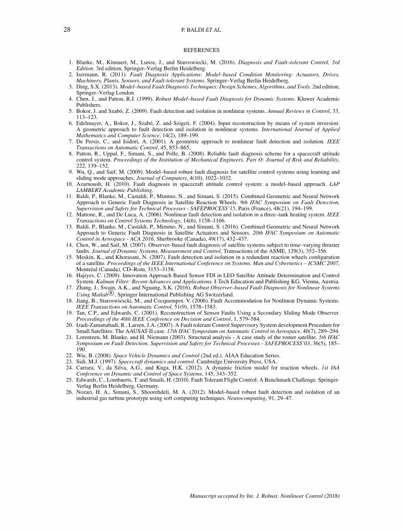
28 P. BALDI ET AL.
REFERENCES
1. Blanke, M., Kinnaert, M., Lunze, J., and Staroswiecki, M. (2016). Diagnosis and Fault–tolerant Control, 3rdEdition. 3rd edition, Springer–Verlag Berlin Heidelberg.
2. Isermann, R. (2011). Fault Diagnosis Applications: Model–based Condition Monitoring: Actuators, Drives,Machinery, Plants, Sensors, and Fault-tolerant Systems. Springer–Verlag Berlin Heidelberg.
3. Ding, S.X. (2013). Model–based Fault Diagnosis Techniques: Design Schemes, Algorithms, and Tools. 2nd edition,Springer–Verlag London.
4. Chen, J., and Patton, R.J. (1999). Robust Model–based Fault Diagnosis for Dynamic Systems. Kluwer AcademicPublishers.
5. Bokor, J. and Szabo, Z. (2009). Fault detection and isolation in nonlinear systems. Annual Reviews in Control, 33,113–123.
6. Edelmayer, A., Bokor, J., Szabo, Z. and Szigeti, F. (2004). Input reconstruction by means of system inversion:A geometric approach to fault detection and isolation in nonlinear systems. International Journal of AppliedMathematics and Computer Science, 14(2), 189–199.
7. De Persis, C., and Isidori, A. (2001). A geometric approach to nonlinear fault detection and isolation. IEEETransactions on Automatic Control, 45, 853–865.
8. Patton, R., Uppal, F., Simani, S., and Polle, B. (2008). Reliable fault diagnosis scheme for a spacecraft attitudecontrol system. Proceedings of the Institution of Mechanical Engineers, Part O: Journal of Risk and Reliability,222, 139–152.
9. Wu, Q., and Saif, M. (2009). Model–based robust fault diagnosis for satellite control systems using learning andsliding mode approaches. Journal of Computers, 4(10), 1022–1032.
10. Azarnoush, H. (2010). Fault diagnosis in spacecraft attitude control system: a model–based approach. LAPLAMBERT Academic Publishing.
11. Baldi, P., Blanke, M., Castaldi, P., Mimmo, N., and Simani, S. (2015). Combined Geometric and Neural NetworkApproach to Generic Fault Diagnosis in Satellite Reaction Wheels. 9th IFAC Symposium on Fault Detection,Supervision and Safety for Technical Processes - SAFEPROCESS’15, Paris (France), 48(21), 194–199.
12. Mattone, R., and De Luca, A. (2006). Nonlinear fault detection and isolation in a three–tank heating system. IEEETransactions on Control Systems Technology, 14(6), 1158–1166.
13. Baldi, P., Blanke, M., Castaldi, P., Mimmo, N., and Simani, S. (2016). Combined Geometric and Neural NetworkApproach to Generic Fault Diagnosis in Satellite Actuators and Sensors. 20th IFAC Symposium on AutomaticControl in Aerospace - ACA 2016, Sherbrooke (Canada), 49(17), 432–437.
14. Chen, W., and Saif, M. (2007). Observer–based fault diagnosis of satellite systems subject to time–varying thrusterfaults. Journal of Dynamic Systems, Measurement and Control, Transactions of the ASME, 129(3), 352–356.
15. Meskin, K., and Khorasani, N. (2007). Fault detection and isolation in a redundant reaction wheels configurationof a satellite. Proceedings of the IEEE International Conference on Systems, Man and Cybernetics – ICSMC 2007,Montreal (Canada), CD–Rom, 3153–3158.
16. Hajiyev, C. (2009). Innovation Approach Based Sensor FDI in LEO Satellite Attitude Determination and ControlSystem. Kalman Filter: Recent Advances and Applications. I-Tech Education and Publishing KG, Vienna, Austria.
17. Zhang, J., Swain, A.K., and Nguang, S.K. (2016). Robust Observer–based Fault Diagnosis for Nonlinear SystemsUsing Matlab R©, Springer International Publishing AG Switzerland.
18. Jiang, B., Staroswiescki, M., and Cocquempot, V. (2006). Fault Accommodation for Nonlinear Dynamic Systems.IEEE Transactions on Automatic Control, 51(9), 1578–1583.
19. Tan, C.P., and Edwards, C. (2001). Reconstruction of Sensor Faults Using a Secondary Sliding Mode Observer.Proceedings of the 40th IEEE Conference on Decision and Control, 1, 579–584.
20. Izadi-Zamanabadi, R., Larsen, J.A. (2007). A Fault tolerant Control Supervisory System development Procedure forSmall Satellites: The AAUSAT-II case. 17th IFAC Symposium on Automatic Control in Aerospace, 40(7), 289–294.
21. Lorentzen, M. Blanke, and H. Niemann (2003). Structural analysis - A case study of the romer satellite. 5th IFACSymposium on Fault Detection, Supervision and Safety for Technical Processes - SAFEPROCESS’03, 36(5), 185–190.
22. Wie, B. (2008). Space Vehicle Dynamics and Control (2nd ed.). AIAA Education Series.23. Sidi, M.J. (1997). Spacecraft dynamics and control. Cambridge University Press, USA.24. Carrara, V., da Silva, A.G., and Kuga, H.K. (2012). A dynamic friction model for reaction wheels. 1st IAA
Conference on Dynamic and Control of Space Systems, 145, 343–352.25. Edwards, C., Lombaerts, T. and Smaili, H. (2010). Fault Tolerant Flight Control: A Benchmark Challenge. Springer-
Verlag Berlin Heidelberg, Germany.26. Nozari, H. A., Simani, S., Shoorehdeli, M. A. (2012). Model–based robust fault detection and isolation of an
industrial gas turbine prototype using soft computing techniques. Neurocomputing, 91, 29–47.
Manuscript accepted by Int. J. Robust. Nonlinear Control (2018)