fast performance uncertainty estimation via...

EARTHQUAKE ENGINEERING AND STRUCTURAL DYNAMICSEarthquake Engng Struct. Dyn. 2009; 00:1–16 Prepared using eqeauth.cls [Version: 2002/11/11 v1.00]

Fast Performance Uncertainty Estimationvia Pushover and Approximate IDA‡

Michalis Fragiadakis1,∗,†, Dimitrios Vamvatsikos2

1 School of Civil Engineering, National Technical University of Athens, GreeceDepartment of Civil Engineering, University of Thessaly, Volos, Greece

2 Department of Civil and Environmental Engineering, Univerisity of Cyprus, Nicosia 1678, Cyprus

SUMMARY

Approximate methods based on the static pushover are introduced to estimate the seismic performanceuncertainty of structures having non-deterministic modeling parameters. At their basis lies the useof static pushover analysis to approximate Incremental Dynamic Analysis (IDA) and estimate thedemand and capacity epistemic uncertainty. As a testbed we use a nine-storey steel frame havingbeam hinges with uncertain moment-rotation relationships. Their properties are fully described bysix, randomly distributed, parameters. Using Monte Carlo simulation with latin hypercube sampling,a characteristic ensemble of structures is created. The Static Pushover to IDA (SPO2IDA) softwareis used to approximate the IDA capacity curve from the appropriately post-processed results of thestatic pushover. The approximate IDAs allow the evaluation of the seismic demand and capacity forthe full range of limit-states, even close to global dynamic instability. Moment estimating techniquessuch as Rosenblackth’s point estimating method and the first-order, second-moment (FOSM) methodare adopted as simple alternatives to obtain performance statistics with only a few simulations. Thepushover is shown to be a tool that combined with SPO2IDA and moment estimating techniques cansupply the uncertainty in the seismic performance of first-mode dominated buildings for the full rangeof limit-states, thus replacing semi-empirical or code tabulated values (e.g. FEMA-350), often adoptedin performance-based earthquake engineering. Copyright c© 2009 John Wiley & Sons, Ltd.

key words: Epistemic Uncertainty; Static Pushover Analysis; Incremental Dynamic Analysis;

Simulation; Moment estimating methods; performance-based earthquake engineering.

1. INTRODUCTION

Structural analysis is plagued by both aleatory randomness, e.g. natural ground motionrecord variability, and epistemic uncertainty, stemming from modeling assumptions or errors.Design codes recognize the importance of uncertainty in the process of seismic design by

∗Correspondence to: Michalis Fragiadakis, Iroon Polutexneiou St., Zografou 15780, Athens, Greece.†E-mail: [email protected]‡Based on a short paper presented at the 14th World Conference on Earthquake Engineering, Beijing, China,2008.

Copyright c© 2009 John Wiley & Sons, Ltd.

2 M. FRAGIADAKIS & D. VAMVATSIKOS

implicitly including generic safety factors in the model, the material properties and the loads.Unfortunately little data is available on the seismic demand and capacity epistemic uncertainty,an issue that is ultimately dealt with tabulated values. Epistemic uncertainty usually receiveslittle attention due to the inherent difficulties and the computational cost in estimating it.Since both randomness and uncertainty are important factors in performance-based earthquakeengineering, efficient estimation methods are always desirable.

Perhaps the first guideline that explicitly treats uncertainty in seismic design is FEMA-350 (SAC/FEMA 2000 [1]). The SAC/FEMA project caused the widespread adoption of thenotion of uncertainty in earthquake engineering applications, and became a major motivationto study rational ways to include the uncertainty in performance estimation. Cornell et al.[2] formed the background of the SAC/FEMA approach for the probabilistic assessment ofsteel frames which allows the inclusion of epistemic uncertainties simply by considering thedispersion they cause on the median demand and capacity. Such concepts have been furtheradvanced by Baker and Cornell [3] who build upon the framework of the Pacific EarthquakeEngineering Research (PEER) Center to propagate the uncertainty from the model to thedecision variables (e.g., losses) using FOSM methods. Other efforts extend the SAC/FEMAapproach to the assessment of reinforced concrete buildings [4] or the development of decision-making tools for the conceptual design of engineering facilites [5].

Although structural reliability analysis methods have considerably evolved during the lastfew years (e.g., [6]) the need for new approaches to estimate uncertainty for complex nonlinearstructures still exists. Monte Carlo simulation methods are powerful tools that can handlealmost any problem, but they always come at the expense of a large number of computationally-intensive nonlinear response history analyses. Other approximating methods such as first andsecond-order reliability methods (FORM, SORM) have been successfully implemented for thecalculation of safety factors in most recent design code procedures, but for structures subjectedto large nonlinear deformations and transient actions, such methods are plagued by the needfor a failure function [6, 7].

For earthquake engineering applications, one method to handle the aleatory uncertaintyintroduced by seismic loading is the Incremental Dynamic Analysis (IDA) [8]. IDA essentiallyrequires multiple nonlinear response history analyses with a suite of ground motion records toprovide a full-range performance assessment, from the early elastic limit-states to the onsetof collapse. To account for other sources of uncertainty, the IDA approach can be combinedwith reliability analysis methods such as Monte Carlo simulation. Such methods have beenpioneered by Dolsek [9] who proposed using Monte Carlo simulation with efficient LatinHypercube Sampling (LHS) on IDA and Liel et al. [10] that used IDA and Monte Carlo orFOSM with a response surface approximating method to study parameter uncertainty. Morerecently, Vamvatsikos and Fragiadakis [11] have also discussed an IDA-based approach and thepossibility of reducing the computational effort by adopting approximate, moment-estimatingmethods. Although such IDA-based methods are powerful, they necessitate the execution ofa large number of nonlinear response history analyses and therefore are beyond the scope ofmany practical applications. While the above publications propose alternative approaches anddiscuss either implicitly or explicitly the issue of computing cost, they all use nonlinear responsehistory analysis under multiple ground motion records. Clearly this may not be feasible at thepresent time for practical, non-academic, applications. Simpler analysis methods are neededthat can provide estimates of the response statistics with minimum computing resources.

Given the computational obstacles, the usual practice to circumvent this problem is by

Copyright c© 2009 John Wiley & Sons, Ltd. Earthquake Engng Struct. Dyn. 2009; 00:1–16Prepared using eqeauth.cls

PERFORMANCE UNCERTAINTY ESTIMATION USING STATIC PUSHOVER METHODS 3

assuming ad hoc values for the dispersions caused by uncertainties, e.g. in the model properties,and either implicitly taking them into account or explicitly including them in the guidelines,as in FEMA-350. For example, Yun et al. [12] discuss the rationale behind the tabulatedvalues of the FEMA-350 [1] guidelines. Evidently, the proposed parameters are semi-empiricallyderived from a limited number of benchmark structures. These values can be seen as reasonableplaceholders that, unfortunately, in the absence of more rational and proven values, tend tobecome the de facto standard.

In search for a compromise, we propose a novel methodology for estimating responsestatistics using static pushover analysis. During the past few years, static pushover methods(SPO) have become common in the earthquake engineering practice [13, 14] and thereforethis analysis approach lies in the core of the methods we are proposing. Furthermore,a single static pushover requires considerably less computational resources compared tothe hundreds response history analyses of an actual multi-record IDA that are practicallybeyond the scope of most projects. Similarly to IDA, our method maintains a full-rangeperformance evaluation capability using as link between SPO and IDA an R − µ − T (forcereduction factor - ductility - period) relationship, known as Static Pushover to IncrementalDynamic Analysis (SPO2IDA)[15, 16]. SPO2IDA is an R − µ − T relationship that offersaccurate prediction capabilities even close to collapse using, instead of bilinear elastoplastic, amultilinear approximation of the static pushover envelope. Having such a tool at our disposalwe can quickly perform all the necessary simulations and obtain an estimate of the effectof uncertainty on the demand and capacity of structures. Using a nine-storey steel frameas a reference structure we will employ Monte Carlo simulation and moment-estimationtechniques together with static pushover and SPO2IDA to achieve rapid evaluation of theseismic performance variability due to epistemic uncertainty in our model parameters.

2. STRUCTURAL MODELS

The structure considered is a nine-storey steel moment-resisting frame with a singe-storeybasement, shown in Figure 1. The frame has been designed according to 1997 NEHRP(National Earthquake Hazard Reduction Program) provisions for a Los Angeles site. We use acenterline model with nonlinear connections created at the OpenSees [17] platform. The beamsare modelled with lumped-plasticity elements, thus allowing the formation of plastic hingesat the two beam ends. The columns are considered elastic, consistent with a strong-column,weak-beam design. Preliminary testing has shown that cases where column yielding occursare isolated and therefore this choice has a negligible effect on the accuracy of model while itconsiderably reduces its complexity. Geometric nonlinearities have been incorporated in theform of P−∆ effects, while the internal gravity frames have been explicitly modeled (Figure 1).In effect, this is a first-mode dominated structure with a fundamental period of T1 = 2.35sand a modal mass equal to 84% of the total mass that still allows for a significant sensitivityto higher modes.

The connections are modeled using the “Hysteretic material” of the OpenSees library[17]. This is a uniaxial moment-rotation relationship that allows modelling the fracturingconnections with rotational springs having moderately pinching hysteresis and a quadrilinearbackbone, shown in normalised coordinates in Figure 2 (see also reference [18]). The randomparameters considered refer to the properties of the quadrilinear backbone curve, which initially



Figure 1. The LA9 steel moment-resisting frame.

Table I. Random parameters and their statistics.

Mean c.o.v Lower Upperbound bound

aMy 1.0 0.20 0.70 1.30ah 0.1 0.40 0.04 0.16µc 3.0 0.40 1.20 4.80ac -0.5 0.40 -0.80 -0.20r 0.5 0.40 0.20 0.80µu 6.0 0.40 2.40 9.60

allows for elastic behavior up to aMy times the nominal yield moment My, then hardens at anon-negative normalised slope of ah and terminates at a rotational ductility µc. Beyond thispoint, a negative stiffness segment starts having a normalised slope ac. The residual plateauappears at a normalised height r, delaying the failure of the connection until the ultimaterotational ductility µu. Thus to completely describe the backbone of the monotonic envelopeof the hinge moment-rotation relationship, six parameters are necessary: aMy, ah, µc, ac, rand µu, assuming similar behavior for both positive and negative moments. This is essentiallya complex backbone that is versatile enough to simulate the behavior of numerous moment-connections. Other sources of epistemic uncertainty (e.g. stiffness and/or mass uncertainty)are not examined here, although our methodology can be easily extended to those parametersalso.

The backbone properties of the plastic hinges are considered as random variables and hence



are the only source of epistemic uncertainty. The parameters are modeled to be independentlynormally distributed with mean and coefficient of variation (c.o.v) as shown in Table I. Themean values represent best estimates of the backbone parameters, while the c.o.v values wereassumed, since for most parameters there is no explicit guidance in the literature. Thus we useda c.o.v equal to 40% for all the parameters except for the yield moment where 20% was usedinstead. To avoid assigning the random parameters with values with no physical meaning, e.g.ah > 1, or r < 0, their distribution is appropriately truncated within 1.5 standard deviationsas shown in Table I. All distributions were appropriately rescaled to avoid the concentrationof high probabilities at the cutoff points. The resulting connection model is flexible enoughto range from fully-ductile, nearly elastoplastic connections (e.g. r = 0.80, µu = 9) down tooutright brittle cases that suddenly fracture at low ductilities (e.g. µu = 2.4).

To account for parameter uncertainty stemming from the properties of the connectionsof a steel moment frame, the plastic hinge properties can be varied simultaneously for thewhole structure, or individually, by applying local changes to several connections. In thelater case the precise locations of the connections are randomly assigned thus assessing theglobal performance when the capacity of a number of connections is uncertain e.g. due topoor manufacturing or localised phenomena. Luco and Cornell [19] studied the response ofmoment-resisting frames with random fracturing connections typical to those of pre- and post-Northridge steel buildings. On the other end, varying together the properties of every frameconnection, i.e. assuming that all have the same normalised properties, is expected to have amore pronounced effect on the response, pinpointing the influence of each of the six parameterson the global capacity. This scenario is the one we are going to adopt as it is consistent withthe case where the engineer does not have sufficient data for the individual moment-rotationbackbones and their spatial correlation, thus his/her model relies on empirical values andjudgment.

3. PERFORMANCE EVALUATION WITH THE STATIC PUSHOVER TOINCREMENTAL DYNAMIC ANALYSIS TOOL

3.1. Incremental Dynamic Analysis

Incremental Dynamic Analysis (IDA) is a powerful analysis method that offers thoroughseismic demand and capacity prediction capability [8]. It involves performing a series ofnonlinear response history analyses under a multiply scaled suite of ground motion records.By selecting proper Engineering Demand Parameters (EDPs) to characterise the structuralresponse and choosing an Intensity Measure (IM), e.g. the 5%-damped, first-mode spectralacceleration Sa(T1, 5%), to represent the seismic intensity, we can generate the IDA curves ofEDP versus IM for every record and then estimate the 16%, 50% and 84% summarised curves.The EDP typically adopted is the maximum interstorey drift, θmax, that previous researchhas shown that is a good measure of structural damage, while other EDPs can be adopted asin cases where non-structural acceleration-sensitive damage is of interest. On the IDA curvesthe desired limit-states (e.g., immediate occupancy or collapse prevention according to [1]) canbe defined by setting appropriate limits on the EDPs and then estimating the correspondingcapacities and their probabilistic distributions. Such results combined with probabilistic seismichazard analysis [8] allow the estimation of mean annual frequencies (MAFs) of exceeding the



0 10

1

normalized rotation, ! / !yield

norm

aliz

ed m

omen

t, M

/ M

yiel

d

µc(3) µu(6)

ah(10%) ac(−50%)

r (50%)

Figure 2. The moment-rotation relationship of the beam point-hinge in normalised coordinates.

limit-states (e.g. reference [20]) thus offering a direct characterization of seismic performance.Even for simple structures, IDA comes at a considerable cost, since it requires the use ofmultiple nonlinear response history analyses that are usually beyond the abilities and thecomputational resources of the average practicing engineer. Therefore, a simpler and fasteralternative is always desirable.

Figure 3a shows thirty single-record IDA curves for the LA9 steel frame. Each curve has beenobtained from fourteen response history analyses using the hunt-and-fill algorithm and theninterpolating with appropriate splines [20]. The table of the ground motion records used forthis analysis is given in reference [11]. In Figure 3a, the collapse limit-state appears at a θmaxvalue approximately equal to 0.1, signifying the initiation of the flatline branch. The thirtysingle-record IDAs are summarised to produce the median and the 16%, 84% percentile curvesof Figure 3b. The median, or 50% fractile, provides a ‘central’ capacity curve, while the 16%,84% percentiles give a measure of the dispersion around the median. The fractile capacitiescan be summarised either in terms of Sa(T1, 5%) with respect to θmax, i.e. Sa(T1, 5%)|θmax, orin terms of θmax given the spectral acceleration Sa(T1, 5%), i.e. θmax|Sa(T1, 5%). In practice[20] and provided that a reasonably large number of records is used, both approaches areexpected to yield equivalent results (Figure 3b) and therefore the final choice of the post-processing method depends on the problem at hand. In the remainder of the paper we mainlyconcentrate on the Sa-capacity given θmax statistics, but this does not restrict our methodologysince our results can be easily translated to θmax-demand given the IM statistics.

3.2. Static Pushover to Incremental Dynamic Analysis (SPO2IDA)

IDA is a comprehensive, yet computer-intensive method. It is possible to approximate theresults of IDA both for single and for multi-degree-of-freedom systems utilising informationfrom the force-deformation envelope (or backbone) of the static pushover to generate thesummarised 16%, 50% and 84% IDA curves [15, 16]. The prediction is based on the study ofnumerous SDOF systems having a wide range of periods, moderately pinching hysteresis and5% viscous damping, while they feature backbones ranging from simple bilinear to complexquadrilinear, as shown in Figure 2. Having compiled the results into the SPO2IDA tool,



available online [21] we can get an approximate estimate of the performance of virtually anyoscillator without having to perform the costly analyses, and quickly recreate the fractile IDAs.SPO2IDA is in essence an R − µ − T relationship that will provide not only central values(mean or median) but also the dispersion, due to record-to-record aleatory randomness, usingonly a multilinear approximation of the static pushover curve.

For SDOF structures, IDA curves can be appropriately represented in normalizedcoordinates of the strength reduction factor R, versus the ductility µ. The strength reductionfactor R is defined as the ratio Sa(T1, 5%)/Syielda (T1, 5%), where Syielda (T1, 5%) is theSa(T1, 5%) value to cause first yield, while the ductility, µ, is the oscillator’s displacement,δ, normalised by the yield displacement, δyield. Thus once the period and the properties of theforce-deformation relationship are known for the SDOF system, SPO2IDA directly providesits median and the 16, 84% fractile demand and capacity in normalised R, µ coordinates.

0 0.05 0.1 0.15 0.20

0.2

0.4

0.6

0.8

1

1.2

1.4

1.6

1.8

maximum interstorey drift ratio, !max

"firs

t−m

ode"

spe

ctra

l acc

eler

atio

n S a(T

1,5%

) (g)

(a)

0 0.05 0.1 0.15 0.20

0.2

0.4

0.6

0.8

1

1.2

1.4

1.6

1.8


"firs

t−m

ode"

spe

ctra

l acc

eler

atio

n S a(T

1,5%

) (g)

16% demand / 84% capacity



fractiles of !max given Safractiles of Sa given !max

(b)

Figure 3. Incremental Dynamic Analysis (IDA) curves for the LA9 steel structure: (a) thirty single-record IDAs, and (b) summarisation of the thirty IDA curves into their fractile curves of θmax given

Sa(T1, 5%), or Sa(T1, 5%) given θmax.

3.3. SPO2IDA for multi-degree of freedom systems (MDOF)

The SPO2IDA tool has been extended to first-mode dominated MDOF structures [16], enablingan accurate estimation of the fractile IDA curves even close to collapse without the need of anynonlinear response history analysis. In addition, it has been shown to only slightly increasethe error in our estimation, resulting to an accuracy that can be compared to that of theactual IDA using a smaller number, e.g. ten, ordinary ground motion records. Thus SPO2IDAcan approximate the summarized IDA results, offering an efficient and simple method forestimating the uncertainty associated with the limit-state capacities, given the variability inthe backbone parameters of the beam plastic hinges. In the following paragraphs we explain indetail its application on our testbed structure and we propose a simplified method (comparedto reference [16]) that can be used for epistemic uncertainty estimations within Monte Carlo.

The application of the SPO2IDA tool on the base-case, mean-parameter model of the LA9



0 0.01 0.02 0.03 0.04 0.05 0.06 0.070

2000

4000

6000

8000

10000

12000

roof drift ratio, !roof

base

she

ar (k

N)

trilinear modelquadrilinear modelSPO

(a)

0 1 2 3 4 5 6 7 80

0.5

1

1.5

2

2.5

3

3.5

4

4.5

5

ductility, µ=!/!yield

stre

ngth

redu

ctio

n fa

ctor

, R=S

a/Sayie

ld

FEMA−440SPOSPO2IDA (trinlinear)SPO2IDA (quadrilinear)

(b)

Figure 4. (a) The SPO curve for a nine-storey steel structure and its approximation with differentmultilinear models, (b) SPO2IDA predictions for the trilinear and the quadrilinear approximations of

the SPO in R,µ coordinates.

moment-resisting steel structure is schematically shown in Figure 4. The process involvesapproximating the static pushover curve with a multilinear envelope to allow extractingthe properties of the backbone curve (Figure 4a). The complete theoretical justification anddiscussion on the application of SPO2IDA on MDOF structures can be found in [16]. Typicallyfor first-mode dominated structures, SPO2IDA allows the use of a bilinear, trilinear or fullquadrilinear approximation of the structure’s pushover curve. While the accuracy of theapproximation rises accordingly, so does the complexity of the automated fitting algorithmto estimate the appropriate parameters, an issue that we discuss in the section that follows.For the sake of comparison, we will attempt both a trilinear and a quadrilinear fit as shown,e.g. in Figure 4a.

The choice of the lateral load pattern has a significant effect on the SPO envelope andtherefore Vamvatsikos and Cornell [16] report that the proper application of SPO2IDA onMDOF structures entails the identification of the most-damaging lateral load pattern. Forthis realisation of the LA9 steel frame it was found that a triangular or a first-mode patternwill provide sufficiently accurate results, close to the worst-case scenario. Thus we are sparedthe need to search for the most damaging pattern for every realisation of the structure inthe Monte Carlo simulation. In the general case, alternative lateral load patterns have to betested for every frame realisation to find the one that seems to be the most damaging. For themethodology discussed here, this has to be performed only for the base-case, mean parameterstructure.

Moreover, although SPO2IDA provides all three 16,50,84% fractile curves, we may simplifyits application by using only the 50% curve together with the typical first-order assumption [22],where the base-case mean parameter model is assumed to provide the overall mean/medianresponse and the parameter uncertainty is only considered to add variability around thismean/median. This was shown by Vamvatsikos and Fragiadakis [11] to be a viable assumptionfor this structure, thus, in the interest of simplicity, this will be our main proposal. Nevertheless,



the ability to compute the 16 and 84% fractiles allows the application of this method in a moregeneral sense.

Having approximated the SPO curve, the backbone parameters can be easily extracted.Following the terminology of SPO2IDA (for a backbone description similar to that of Figure 2)the extracted parameters will be: FSPOy (instead of My in Figure 2), aSPOh , µSPOc , aSPOc . For

the trilinear approximation rSPO is set equal to zero and µSPOu is defined as the intersectionof the horizontal axis with the descending branch, while for the quadrilinear model they areextracted from the SPO as the remaining parameters. The six parameters are then given asinput to SPO2IDA to produce the median capacities shown in Figure 4b.

Figure 4b shows in R− µ coordinates the SPO2IDA-produced capacities together with thecorresponding SPO. The difference between the trilinear and the quadrilinear approximationis the truncation of the tail of the SPO (Figure 4a) which results to a slight underestimation ofthe R capacity when the trilinear model is adopted. Figure 4b also shows the capacity predictedwith a simpler code-prescribed R−µ−T relationship, such as that of the FEMA-440 guidelines[14]. For medium to long periods (typically T1 ≥ 1) almost every such relationship follows theequal-displacement rule and thus the ratio of R over µ is equal to one. FEMA-440 also setsan upper limit on the maximum R-value considerable, Rmax, which adopting the notation ofthis paper is calculated as follows:

Rmax = µSPOh +(αSPOc )−t

4(1)

where t = 1 + 0.15 ln(T1). FEMA-440 uses this limit to introduce the physical bounds ofthe R − µ − T relationship indicating that when Rmax is exceeded more elaborate methodsof analysis need to be considered. This relationship can be considered as an alternative toSPO2IDA that can be implemented at a 30-40% underestimation in the near collapse region(Figure 4b.)

Since the capacities of SPO2IDA are in dimensionless R − µ coordinates, they need to bescaled to another pair of IM, EDP coordinates, more appropriate for MDOF systems, suchas the Sa(T1, 5%) and the maximum interstorey drift ratio θmax. The scaling from R − µ toSa(T1, 5%)− θmax is performed with simple algebraic calculations:

Sa(T1, 5%) = R · Syielda (T1, 5%) (2)

θroof = µ · θyieldroof (3)

where the bold font denotes a vector. Once θroof is known, θmax can be extracted from theresults of the SPO, since for every load increment the correspondence between the two EDPsis always available.

Prior to applying Equations 2 and 3 we have to determine the values of Sa(T1, 5%) andθroof at yield. This task is trivial for SDOF systems, but it is not straightforward for MDOFstructures mainly due to the effect of higher modes. Some records will force the structure toyield earlier and others later, thus yielding will always occur at different levels of Sa(T1, 5%) andθroof. Driven by our approximation to the SPO curve, we let the yield roof drift, θroof, be definedas the apparent yield point of the multilinear approximation. This assumption is not strictlytrue for MDOF structures and it becomes highly accurate only if the first mode is dominant,but it is sufficient for our purpose. Therefore, the accurate estimation of Syielda (T1, 5%) comesdown to approximating the elastic “slopes” of the median IDA curves plotted with θroof as the



0 0.05 0.1 0.15 0.20

0.2

0.4

0.6

0.8

1

1.2


"firs

t−m

ode"

spe

ctra

l acc

eler

atio

n S a(T

1,5%

) (g)

50% IDAFEMA−440SPO2IDA trilinear fitSPO2IDA quadrilinear fit

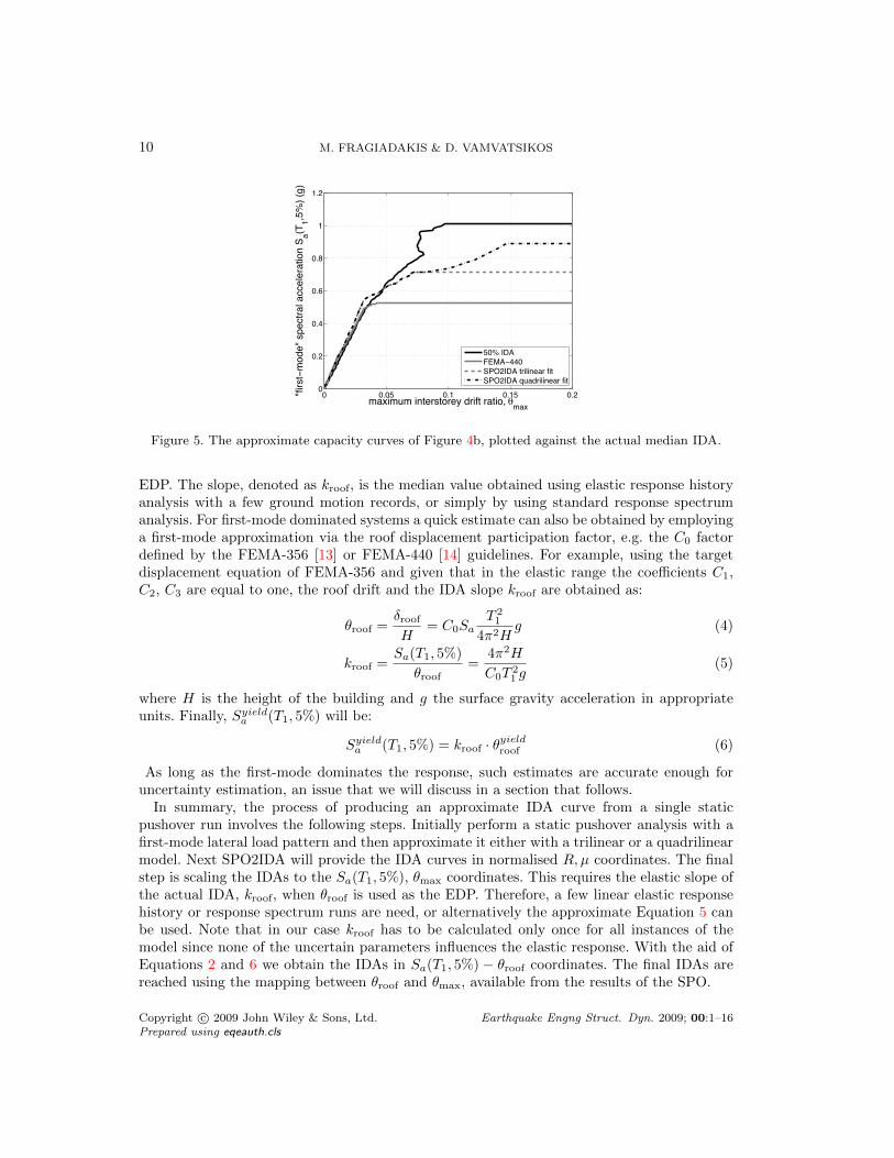
Figure 5. The approximate capacity curves of Figure 4b, plotted against the actual median IDA.

EDP. The slope, denoted as kroof, is the median value obtained using elastic response historyanalysis with a few ground motion records, or simply by using standard response spectrumanalysis. For first-mode dominated systems a quick estimate can also be obtained by employinga first-mode approximation via the roof displacement participation factor, e.g. the C0 factordefined by the FEMA-356 [13] or FEMA-440 [14] guidelines. For example, using the targetdisplacement equation of FEMA-356 and given that in the elastic range the coefficients C1,C2, C3 are equal to one, the roof drift and the IDA slope kroof are obtained as:

θroof =δroof

H= C0Sa

T 21

4π2Hg (4)

kroof =Sa(T1, 5%)

θroof=

4π2H

C0T 21 g

(5)

where H is the height of the building and g the surface gravity acceleration in appropriateunits. Finally, Syielda (T1, 5%) will be:

Syielda (T1, 5%) = kroof · θyieldroof (6)

As long as the first-mode dominates the response, such estimates are accurate enough foruncertainty estimation, an issue that we will discuss in a section that follows.

In summary, the process of producing an approximate IDA curve from a single staticpushover run involves the following steps. Initially perform a static pushover analysis with afirst-mode lateral load pattern and then approximate it either with a trilinear or a quadrilinearmodel. Next SPO2IDA will provide the IDA curves in normalised R,µ coordinates. The finalstep is scaling the IDAs to the Sa(T1, 5%), θmax coordinates. This requires the elastic slope ofthe actual IDA, kroof, when θroof is used as the EDP. Therefore, a few linear elastic responsehistory or response spectrum runs are need, or alternatively the approximate Equation 5 canbe used. Note that in our case kroof has to be calculated only once for all instances of themodel since none of the uncertain parameters influences the elastic response. With the aid ofEquations 2 and 6 we obtain the IDAs in Sa(T1, 5%) − θroof coordinates. The final IDAs arereached using the mapping between θroof and θmax, available from the results of the SPO.



0 0.02 0.04 0.06 0.080

2000

4000

6000

8000

10000

12000

14000

base

she

ar (k

N)

roof drift ratio, !roof0 0.02 0.04 0.06 0.08

0

2000

4000

6000

8000

10000

12000

14000

roof drift ratio, !roof0 0.02 0.04 0.06 0.08

0

2000

4000

6000

8000

10000

12000

14000


SPOtrilinear modelquadrilinear model

Figure 6. Different SPO curves and their multilinear approximation.

For the SPO curve of Figure 4, the median IDA obtained with SPO2IDA and the actual IDAcurve using thirty ordinary ground motion records [11] are shown in Figure 5. For our model,the error in the procedure is typically 10–20%, while the computing time comes down from 2–3hours required for a single IDA to just a couple of minutes for SPO2IDA, approximately twoorders of magnitude less. It is worthwhile to note that compared to the quadrilinear pushoverapproximation, the trilinear curve slightly biases our IDA results towards lower Sa-capacities,the reason being our truncating of the tail of the pushover as shown in Figure 4a. The FEMA-440 relationship is accurate enough only for low elastic and nearly-elastic Sa(T1, 5%) intensitiesthus leaving more elaborate relationships, such as SPO2IDA, to be the only alternative whenapproximate capacity estimations are sought for high intensity, near-collapse levels. The smalldiscrepancies in the elastic range that appear between the four curves of Figure 5 are actually adirect by-product of the elastic IDA-slope determination process. While the FEMA-440 curveseems to be more accurate, there are always small implementation details that can swing theseminor differences either way.

3.4. Fitting the SPO curves

The fitting of a multilinear model on the SPO is not a trivial issue, especially when it has tobe performed without supervision within a Monte Carlo scheme. This issue has already receiveattention as it is discussed in the guidelines [13, 14] to serve purposes seemingly different tothose of our study. For example the FEMA-356 [13] guidelines propose the fitting of a bilinearcurve on the force-displacement relationship to assist calculating the effective stiffness and theyield strength of the whole structure. The effective stiffness is taken as the secant stiffnesscalculated at a base shear equal to 60% of the effective yield strength, while the slope of thepost-elastic segment is chosen so that balance is achieved between the areas above and belowthe SPO data. The FEMA-440 [14] guidelines discuss the fitting of the strength degradingsegment with a line of negative slope αc. It is suggested to separate the effect of P − ∆phenomena by repeating the analysis with and without including them and performing thefitting for each case to obtain the slopes αP−∆, αw/o,P−∆. Then the final slope is calculatedas the weighted sum: αc = αP−∆ + λ(αw/o,P−∆ − αP−∆), where λ is taken 0.2 for a near-field site or 0.8 otherwise. It is evident that the above fitting approaches require engineeringjudgment and are sensitive to non-objective decisions. To serve our purposes the fitting has tobe performed within a software tool and thus we need to develop a generally-applicable androbust algorithm that can fit a multilinear curve on the SPO curve.



The fitting of a trilinear or a quadrilinear model on the SPO depends primarily on theproperties of the SPO curve. Figure 6 shows three different SPO curves that the fittingalgorithm should be able to handle. The plot in the left is the most common where bothtrilinear and quadrilinear models can be fitted, contrary to the case in the middle where theoriginal SPO does not have a residual plateau and therefore only a trilinear curve can be fitted.Finally, the right plot shows a case where the SPO is abruptly terminated due to numericalnon-convergence, signifying a very brittle structure (assuming the analysis has been carefullyperformed). All such cases need to be handled efficiently.

In our implementation, the fitting of the SPO is performed in two distinct phases. The firstphase refers to fitting the elastic and the post-elastic segment until the point where ‘capping’occurs, i.e. the point where the negative segment is initiated. In the second phase we fit the‘post-capping’ segment with slope αc and the residual strength plateau with ordinate r (Figure2). Previous research [11, 16] has revealed that the yield strength and the post elastic stiffness,αhKel, seem to have a significant effect at the SPO-level, but when IDA is performed thesensitivity is small. Therefore the fitting process is simple in this phase and can be done byobtaining the slopes αel and αh of the elastic and the post-elastic segment, respectively, anddefine the yield point as the intersection of the two lines. Alternatively the yielding point canbe defined as the point where the tangent slope reaches for the first time a given percentage(say 50%) of the initial elastic. In our study, both approximations will yield almost equivalentSPO2IDA results.

The post-capping stiffness, αc, and the height of the residual plateau, r, are more difficultto capture, while our results are more sensitive to those parameters. Again two alternativestrategies have been tested. In the first alternative we perform least-square fitting on thepoints between the capping point and the first point of the SPO with base shear lower thanan reasonably-chosen value, say 30%, of the yield strength. Care needs to be taken to scalethe coordinates of the SPO so that the least-square line passes through the capping point.In other words, if V c and θcroof are the coordinates of the capping point and Kel the initialelastic stiffness, the fitted line can be expressed as (V − V c) = ac Kel (θroof − θcroof ). Theresidual strength, r, is obtained by finding the horizontal line that balances the areas betweenthe branch with negative slope ac and the remaining points of the SPO. For a quadrilinearapproximation a second alternative is also available. In this case an iterative process thatpasses through every point of the SPO that lies beyond the capping point is initiated. Trial acand r values are defined by the coordinates of the trial point and the areas above and belowthe approximating lines are calculated. The point where best balance is achieved defines theintersection point of the descending and the horizontal branch. Note that when this processis followed, the abscissas and the ordinates of the SPO need to normalised by their maximumvalues to achieve efficient fitting. In our case, both procedures were found equally efficient,while for our implementation we have adopted the first option. Contrary to FEMA-440 wefound that there is no need to separate the loss in strength caused by P − ∆ effects andthe component in-cycle strength degradation, since our SPO2IDA tool treats both sources ofnonlinearity equally.



4. METHODOLOGY

In order to accurately calculate the performance statistics of a structure using static pushovermethods, we will employ an approach based on the Monte Carlo (MC) simulation with LatinHypercube Sampling (LHS), conceptually following the idea proposed by Dolsek [9]. As simplerand less resource-demanding alternatives we propose methods that rely on moment-estimatingtechniques such as Rosenblackth’s 2K+1 point estimate method (PEM) [?] and the first-order,second-moment method (FOSM) [6, 7].

4.1. Monte Carlo Simulation with Latin Hypercube Sampling (LHS)

Using the Monte Carlo (MC) simulation on top of SPO2IDA we are able to quickly obtain asufficient sample of IDA curves which can be post-processed to provide the required responsestatistics. Since we are interested primarily in the mean and the dispersion of the capacity,the MC method can be combined with the Latin Hypercube Sampling (LHS) method [24] toensure improved accuracy with only a few simulations compared to classic random sampling.As previously discussed, the random variables are the six parameters that fully describe thebackbone of the plastic hinge moment-rotation relationship (Figure 2) and they are variedconcurrently throughout the structure. Using their distribution properties (Table I) we obtainNLHS samples with the aid of the algorithm of Iman and Conover [25] to ensure zero correlationamong the six variables. Each of the NLHS realizations of the LA9 frame is subjected to apushover analysis and then the SPO2IDA tool is utilised to finally obtain NLHS median IDArealizations, as discussed in the previous section.

According to Iman [26], if n3 simulations are required to estimate the variation of a linearfunction with a given level of confidence using Monte Carlo with random sampling, then MonteCarlo with LHS sampling will achieve an equivalent estimate with the same confidence afteronly n simulations. For nonlinear functions, there are no closed-form relationships, but stillLHS would normally require less simulations than random sampling, as long as the sample sizen is large compared to the number of variables K. When the response statistics of buildingssubjected to seismic actions are sought, the accuracy of LHS for our nonlinear structure isexpected to be close to that of a linear system, since the localized nature of nonlinearity(beam-hinging) reduces changes in the stiffness matrix to a minimum. Therefore, the degree ofnonlinearity of the problem is actually quite small. In any case, as discussed in [11] a samplesize of NLHS = 200 Monte Carlo simulations with latin hypercube sampling is expected toprovide a close estimate of the response statistics of the problem considered here, althoughsmaller sample sizes may have been also adequate [9]. A parametric investigation of the requirednumber of Monte Carlo simulations, NLHS, is presented in the last section of the paper.

In our development we are interested in estimating a central value and a dispersion for theSa-values of capacity for a given limit-state defined at a specific value of θmax. As a centralvalue we use the median of the Sa(T1, 5%)-capacities given θmax, ∆Sa|θmax

, while the dispersioncaused by the uncertainty in the median capacity will be characterised by its β-value, [2] , i.e.the standard deviation of the natural logarithm of the median Sa-capacities conditioned onθmax: βU = σlnSa|θmax

. In terms of the work of Jalayer [22] we essentially adopt the IM-basedmethod of estimating the mean annual frequency of limit-state exceedance.

Thus, if lnS ja,50%, j = 1, . . . , NLHS, are the median Sa-capacities for a given value of θmax

and lnSa,50% is the mean of their natural logarithm, we can obtain the overall median and



dispersion, βU , as:

∆Sa =medj

(S ja,50%

)(7)

βU =

√√√√∑j

(lnSja,50% − lnSa,50%

)2

NLHS − 1(8)

where “medj” is the median operator over all indices j.According to the work of Cornell et al. [2], such an estimate of the response dispersion due

to epistemic uncertainty can be combined with the dispersion due to record-to-record aleatoryrandomness with a square-root-sum-of-squares (SRSS) rule to provide the total variability:

βRU =√β2R + β2

U (9)

This assumption has seen much use and it has been shown to work reasonably well for thisstructure [11]. Alternatively, one could take advantage of SPO2IDA’s ability to provide boththe central value and the dispersion of demand and capacity due to aleatory randomnessto allow a more precise estimation of the overall variablity βRU . By assuming a lognormaldistribution of capacity Sa given θmax, the 50% IDA will provide the median while the 16 and84 fractile IDAs allow us the estimation of its dispersion, for every sample and every value ofθmax. Thus, for every sample structure we can draw 30 (or more) random IDA curves accordingto the distribution properties prescribed by the 16, 50 and 84% percentiles. Then we can pooltogether the results from all NLHS = 200 samples and compute the overall median and βRUfrom the 30 × 200 = 6000 single-record Sa|θmax IDA curves, much in the way that was doneby Vamvatsikos and Fragiadakis [11] for the actual IDA runs. As the results will show, thislevel of sophistication is not necessary for our case-study.

4.2. Approximate Moment Estimation

A simpler alternative to performing Monte Carlo simulation is the use of moment-estimatingmethods to approximate the variability in the IDA results. Such methods are typically based ona small number of runs for appropriately perturbed versions of the structural model obtainedwith the mean parameter values. Using functional approximations or moment-matching, suchschemes manage to propagate uncertainty from the parameters to the final results using onlya few IDA runs. Specifically in this study we investigate the point estimate method (PEM) ofRosenlueth [?] and the first-order, second-moment method (FOSM) [7, 6]. Other methods thatprobably could be adopted, but have not been examined here, are response surface methods(e.g. [10]), or moment matching [27]. For uncorrelated and unskewed random variables, bothPEM and FOSM need only two IDA evaluations per parameter, spaced one standard deviationaway from the base-case mean structural model obtained using the mean parameter values.Thus to calculate ∆Sa

and βU conditional on θmax we need only 2K + 1 = 13 simulations fora problem with K = 6 random variables.

While both methods are geared towards estimating the mean and the standard deviationof a function, they can be made to produce median and β-dispersion estimates. We only needto apply them to the lnSa(T1, 5%) values rather than Sa(T1, 5%). Then PEM and FOSM willprovide the mean of the natural logarithm of Sa(T1, 5%) and its standard deviation. The latteris exactly the definition of βU while if we take the exponential (exp) of the former and assuming



that lognormality holds, we will get an approximation of the median Sa(T1, 5%). Although thedescription of both methods can be found in standard textbooks the reader is advised to followthe implementation described in Reference [11], as there may be several misunderstandings orerrors when such methods are adopted in a lognormal setting.

5. NUMERICAL RESULTS

To test the validity of the approximating procedures we first applied Monte Carlo simulationusing an actual multi-record IDA with thirty ordinary records on the nine-storey, steel moment-resisting frame of Figure 1. Therefore, we have obtained the exact seismic performance metricsin IDA-terms of NLHS = 200 realizations of the nine-storey frame. The response statisticsobtained with the actual IDA are considered as a reference solution that our approximateSPO-based estimations have to comply with. The Table of ground motion records adopted canbe found in Reference [11].

Figure 7a shows the NLHS =200 static pushover curves for the different realizations of thesteel frame. The ultimate capacity varies between 7000 and 15000kN and yielding practicallyoccurs for θroof values between 0.01 and 0.02. Significant scatter seems to exist in the initiationof the negative branch, while the negative slope itself does not seem to vary considerably. Basedon the established connection between pushover and IDA, these observations lead us to expecta significant post-yield scatter of the IDA results.

Figure 7b shows the median IDAs that compare to the approximate IDAs generated withthe SPO2IDA tool and are shown in Figure 8. Similarly to the median curves of Figure 5,the SPO2IDA curves are smoother than the actual IDA because of the simple backbones andthe smooth parametric equations used in the SPO2IDA tool for both the trilinear and thequadrilinear approximations of Figure 8. For both SPO2IDA approximations the horizontalflatline branch of the ultimate Sa-capacities varies similarly between 0.4g and 1.2g and ispractically always initiated beyond θmax = 0.07. On average, yielding takes place for θmax

values between 0.03 and 0.08, both for the IDA and the SPO2IDA results. While the scatteris similar between IDA and SPO2IDA, the central Sa values are somewhat higher for IDA, anobservation that seems to be slightly demoted when the quadrilinear approximation is used.Furthermore, compared to the trilinear model the IDAs of the quadrilinear approximationshow a slower transition from the initial linear elastic slope to the ultimate capacity flatline.

The IDA and SPO2IDA curves of the Monte Carlo simulation are post-processed to providethe overall median ∆Sa

, and the βU -dispersion conditional on θmax. Figure 9 shows the medianSa-capacities conditional on the limit-state, θmax, where the black lines correspond to thecapacities obtained using Monte Carlo simulation and the gray lines were derived with theapproximating PEM and FOSM methods. Figure 9a corresponds to the median obtained withthe trilinear model and Figure 9b to the quadrilinear approximation. When Monte Carlosimulation is used on top of SPO2IDA (MCSPO2IDA) the conditional median, ∆Sa

, is veryclose to that of the actual IDA for the every limit-state, until θmax = 0.09, while for higherθmax values the agreement is still quite satisfactory for both models. Approaching the collapselimit-states (large θmax values), the error on ∆Sa|θmax

remains constant and approximatelyequal to 16% for the trilinear model, while the quadrilinear model slightly overestimates thecapacity by 6%. For the early and intermediate limit-states (small and intermediate θmax

values), combining PEM and FOSM with SPO2IDA seems to provide a prediction for the



0 0.01 0.02 0.03 0.04 0.05 0.06 0.070

2000

4000

6000

8000

10000

12000

14000

16000


base

she

ar (k

N)

(a)

0 0.05 0.1 0.15 0.20

0.2

0.4

0.6

0.8

1

1.2

1.4


"firs

t−m

ode"

spe

ctra

l acc

eler

atio

n S a(T

1,5%

) (g)

(b)

Figure 7. (a) NLHS=200 static pushover curves for the LA9 nine-storey steel frame, (b) NLHS=200median response curves obtained through IDA.

0 0.05 0.1 0.15 0.20

0.2

0.4

0.6

0.8

1

1.2

1.4


"firs

t−m

ode"

spe

ctra

l acc

eler

atio

n S a(T

1,5%

) (g)

(a)

0 0.05 0.1 0.15 0.20

0.2

0.4

0.6

0.8

1

1.2

1.4


"firs

t−m

ode"

spe

ctra

l acc

eler

atio

n S a(T

1,5%

) (g)

(b)

Figure 8. NLHS=200 IDA curves obtained through SPO2IDA using: (a) a trilinear model, and (b) aquadrilinear model.

median capacities practically identical to that of MCIDA and MCSPO2IDA. However, for limit-states with θmax ≥ 0.1, the prediction of the trilinear approximation with PEM and FOSMslightly biases the median to smaller capacities, while the quadrilinear model underestimatesthe median as approaching collapse. For both models, the moment-estimating methods seemto slightly fluctuate, e.g. the trilinear for θmax values in the 0.04–0.08 range, implying that theestimations of the PEM and the FOSM are less numerically stable compared to those of theMonte Carlo. This numerical behaviour also seems to explain of the error of the quadrilinearmodel for θmax ≥ 0.1. However, for several applications, moment-estimating methods require asmaller number of simulations, thus often justifying their use over the Monte Carlo approach.



0 0.05 0.1 0.15 0.20

0.2

0.4

0.6

0.8

1

1.2


med

ian

S a(T1,5

%), "

S a

MCIDAMCSPO2IDAPEMFOSM

(a)

0 0.05 0.1 0.15 0.20

0.2

0.4

0.6

0.8

1

1.2


med

ian

S a(T1,5

%), "

S a


(b)

Figure 9. Conditional median of Sa given θmax estimated by Monte Carlo on IDA and SPO2IDAversus PEM and FOSM using: (a) a trilinear and (b) a quadrilinear approximation of the SPO.

Figures 10(a-d) show the dispersion βU of the Sa(T1, 5%)-capacities conditioned on θmax

for the two approximating models. As in the case of the medians, the moment-estimatingmethods also exhibit some numerical problems (Figures 10a,b). Since for the β-dispersion thiseffect is more pronounced, we chose to smoothen those curves (Figures 10c,d) using a non-parametric locally weighted regression (LOESS) technique with a coarse span for the movingaverage [28], as also discussed in [11]. Within many practical applications the agreement ofthe methods proposed is quite satisfactory for the whole range of θmax values even whenapproaching collapse, regardless of the approximation of the SPO. More specifically, for thetrilinear model the dispersion at collapse was found close to 0.24 with the MCSPO2IDA approachand 0.29 with the actual IDA, thus resulting to a 17% error, while for the quadrilinear modelthe dispersion was found equal to 0.26, at an error of only 10%. Both figures show that theMCSPO2IDA slightly overestimates βU for θmax lower than 0.07, and underestimates it beyond0.1. PEM and FOSM for θmax values beyond 0.7 provide β-dispersion estimates similar tothat of MCSPO2IDA, underestimating the MCIDA by almost 15% for the trilinear model, whilethe quadrilinear model achieved a close estimation near collapse and an accuracy similar tothe previous methods for θmax between 0.08 and 0.12. Both moment-matching methods canbe seen as approximations to the MCSPO2IDA curve, rather than the MCIDA. Therefore, theunsmoothed data of Figures 10a,b correctly oscillate around the MCSPO2IDA curve for theθmax values less than 0.07, while the smoothed data appear to be closer to the MCIDA, butthis is only due to the coarse span of the LOESS filter.

The accuracy observed in Figure 10 can be partially explained by the small error on theprediction of the median ∆Sa

curves (Figures 5,9), which practically remains constant forevery simulation and was found to be of the order of 10–20%. Since the error in the predictionof the median IDA is relatively consistent from sample to sample, the methods proposed areparticularly suitable for calculating the dispersion due to epistemic uncertainty, βU , whichnormally necessitates more simulations than those required for the median. For example, theelastic slope of the base-case IDA, kroof, (Equation 2) was found approximately equal to 20g



0 0.05 0.1 0.15 0.20

0.05

0.1

0.15

0.2

0.25

0.3


disp

ersio

n, "

U


(a)

0 0.05 0.1 0.15 0.20

0.05

0.1

0.15

0.2

0.25

0.3


disp

ersio

n, "

U


(b)

0 0.05 0.1 0.15 0.20

0.05

0.1

0.15

0.2

0.25

0.3


disp

ersio

n, "

U


(c)

0 0.05 0.1 0.15 0.20

0.05

0.1

0.15

0.2

0.25

0.3


disp

ersio

n, "

U


(d)

Figure 10. Conditional β-dispersion of Sa given θmax estimated with Monte Carlo on IDA andSPO2IDA versus PEM and FOSM using: (a) trilinear model, unsmoothed, (b) quadrilinear model,unsmoothed, (c) trilinear model, smoothed, (d) quadrilinear model, smoothed. The smoothening is

applied only to the PEM and the FOSM methods.

using elastic response history analysis, while the slope calculated with the aid of Equation 4is equal to 25g. While in this simplification there is an obvious bias that seriously affectsthe median (Figure 11a), its consistency over all samples conceals itself on the estimate of thedispersion (Figure 11b). Thus, adopting the first-mode approximate value and a trilinear modelwill result to overestimating the median Sa-capacities for the whole range of θmax values, whilethe estimation of the β-dispersion values is practically unaffected. The findings were similarwhen the quadrilinear model was adopted instead.

Another issue addressed here is the number of latin hypercube samples required for theMonte Carlo method to estimate the median ∆Sa

and the βU -dispersion. We use our trilinearSPO2IDA approximation and with the aid of the Iman and Conover algorithm [25] we generatethree different samples with NLHS=200, 50 and 12. Figure 12 shows the estimations obtained



0 0.05 0.1 0.15 0.20

0.2

0.4

0.6

0.8

1

1.2


med

ian

S a(T1,5

%), "

S a


(a)

0 0.05 0.1 0.15 0.20

0.05

0.1

0.15

0.2

0.25

0.3


disp

ersio

n, "

U


(b)

Figure 11. (a) Conditional median and (b) conditional β-dispersion values using the first-mode estimateof Equation 4 for kroof. Compared to Figure 9 the mean is overestimated, while the estimate of the

dispersion is not affected.

for the different sample sizes. It seems that all three samples provide sufficient estimationsfor the median, while for the βU -dispersion the 200 samples give a slightly better prediction.Therefore, Figure 12 indicates that 12 samples will yield accuracy close to that of the 200samples, and therefore the benefit of NLHS=200 is rather small. If this observation holdsfor any NLHS=12 sample, there would be no need for any moment estimating method sinceMCSPO2IDA is more stable and requires the same number of simulations. To investigate if thisis indeed the case, we generated 50 alternative suites of each of the three NLHS sample sizesand we calculated the 90% confidence intervals for the prediction of the conditional median∆Sa

and the βU -dispersion, using the empirical distribution of the data. Figure 13 shows the90% confidence intervals for the median ∆Sa

and β-dispersion when different sample sizes areadopted. For the median, the 12 samples seem to be sufficient, but certainly the prediction isnot as stable as that of the 200 samples. However, for the βU -dispersion it is clear that the12 simulations are not sufficient and thus the successful prediction of Figure 12b was merelya coincidence.

6. CONCLUSIONS

An innovative approach has been presented to propagate the epistemic uncertainty from themodel parameters to the actual seismic performance of a structure, providing inexpensiveestimates of the response parameters of the limit-state capacities. The methodology proposedhas been applied on a nine-storey, steel moment-resisting frame with beam-column connectionshaving quadrilinear backbones that are fully described by six non-deterministic parameters.Monte Carlo simulation with latin hypercube sampling and moment-estimating techniquesare adopted on top of the Static Pushover to Incremental Dynamic Analysis (SPO2IDA)tool. SPO2IDA provides computationally inexpensive full-range performance estimations,



0 0.05 0.1 0.15 0.20

0.2

0.4

0.6

0.8

1

1.2


med

ian

S a(T1,5

%), "

S a

IDASPO2IDA, NLHS=200SPO2IDA, NLHS=50SPO2IDA, NLHS=12

(a)

0 0.05 0.1 0.15 0.20

0.05

0.1

0.15

0.2

0.25

0.3


disp

ersio

n, "

U

IDASPO2IDA, NLHS=200SPO2IDA, NLHS=50SPO2IDA, NLHS=12

(b)

Figure 12. (a) Conditional median and (b) conditional β-dispersion values using different LHS samplesizes.

0 0.05 0.1 0.15 0.20

0.1

0.2

0.3

0.4

0.5

0.6

0.7

0.8

0.9

1


med

ian

S a(T1,5

%), "

S a

NLHS=200NLHS=50NLHS=12

(a)

0 0.05 0.1 0.15 0.20

0.05

0.1

0.15

0.2

0.25

0.3

0.35


disp

ersio

n, "

U

NLHS=200NLHS=50NLHS=12

(b)

Figure 13. 90% confidence intervals for: (a) conditional median and the (b) conditional β-dispersionvalues using different LHS sample sizes.

approximating the time-consuming IDA. The main findings of the study are:

• The SPO2IDA tool exploits the information contained in a static pushover capacity curveand provides a reliable link between SPO and IDA that can be exploited to obtain usefulresponse statistics for systems with uncertain parameters.

• Moment-estimating techniques require a minimum number of simulations, perturbingeach random variable above and below its mean. Although the Monte Carlo simulationis combined with latin hypercube sampling to ensure good accuracy within a fewsimulations, the number of simulations required is considerably larger compared to that ofmoment-estimating methods. Still, the computing cost of MC on SPO2IDA is affordable



almost for every practical application, since each simulation corresponds to a single staticpushover run.

• Combing Monte Carlo simulation and latin hypercube sampling with SPO2IDA yieldsclose estimates for the median ∆Sa

capacities, only slightly under- or over- estimatingthem when approaching the collapse limit-states. The β-dispersion values of the Sa-capacities are also successfully approximated with only a small error for the higher limit-states.

• Moment-estimating techniques, such as PEM and FOSM, yield equivalent estimationsto those of Monte Carlo on SPO2IDA, the PEM being only marginally more accurate.Compared to the Monte Carlo method they provide similar estimations for both themedian ∆Sa

and the β-dispersion at the expense of only a few static pushover runs. Still,they are prone to numerical difficulties, in our case necessitating the use of smoothingto stabilise their results.

• For the multilinear approximation of the SPO either a trilinear or a quadrilinear modelcan be adopted. Both models will yield practically equivalent results, in our case theformer being more stable but having the tendency to bias the predictions to lowercapacities or smaller β-dispersion values.

• The number of latin hypercube samples NLHS required to obtain the response statisticswith sufficient confidence, depends on the problem at hand. Still, even for our simplecase study with 6 random variables, only relatively large sample sizes, e.g. NLHS ≥ 50,can safeguard the accuracy of Monte Carlo.

The above findings may differ for problems with different building properties, uncertainparameters, or EDPs. However, the methodology discussed is general in scope and whenadjusted to the problem at hand is able to provide results comparable to those of the MonteCarlo on actual IDA, at only a fraction of the cost. All in all, the proposed tool is an excellentresource for approximate estimation of the seismic performance of structures having uncertainsystem properties, for the first time providing specific results for each limit-state that can beused in the place of the generic, code-prescribed values.

REFERENCES

1. FEMA-350. Recommended Seismic Design Criteria for New Steel Moment-Frame Buildings. FederalEmergency Management Agency, Washington DC 2000.

2. Cornell C, Jalayer F, Hamburger R, Foutch D. Probabilistic basis for 2000 SAC/FEMA steel momentframe guidelines. Journal of Structural Engineering 2002; 128(4):526–533.

3. Baker J, Cornell C. Uncertainty propagation in probabilistic seismic loss estimation. Structural Safety2008; 30(3):236–253.

4. Lupoi G, Lupoi A, Pinto P. Seismic risk assessment of RC structures with the ”2000 SAC/FEMA” method.Journal of Earthquake Engineering 2002; 6(4):499–512.

5. Krawinkler H, Zareian F, Medina R, Ibarra L. Decision support for conceptual performance-based design.Earthquake Engineering and Structural Dynamics 2006; 35(1):115–133.

6. Pinto P, Giannini R, Franchin P. Seismic Reliability Analysis of Structures. IUSS Press: Pavia-Italy, 2004.7. Melchers R. Structural Reliability Analysis and Prediction. John Willey, 2002.8. Vamvatsikos D, Cornell C. Incremental dynamic analysis. Earthquake Engineering & Structural Dynamics

2002; 31(3):491–514.9. Dolsek M. Incremental dynamic analysis with consideration of modeling uncertainties. Earthquake

Engineering and Structural Dynamics 2008; doi:10.1002/eqe.869.10. Liel A, Haselton C, Deierlein G, Baker J. Incorporating modeling uncertainties in the assessment of seismic

collapse risk of buildings. Structural Safety 2009; 31(2):197–211.



11. Vamvatsikos D, Fragiadakis M. Incremental Dynamic Analysis for seismic performance uncertaintyestimation. Earthquake Engineering and Structural Dynamics 2009; doi:10.1002/eqe.935.

12. Yun SY, Hamburger R, Cornell C, Foutch D. Seismic performance evaluation for steel moment frames.Journal of Structural Engineering 2002; 128(4):534–545.

13. FEMA-356. Prestandard and commentary for the seismic rehabilitation of buildings. Federal EmergencyManagement Agency, Washington DC 2000.

14. FEMA-440. Improvement of Nonlinear Static Seismic Analysis Procedures. Federal EmergencyManagement Agency, Washington DC 2005.

15. Vamvatsikos D, Cornell C. Direct estimation of the seismic demand and capacity of oscillators with multi-linear static pushovers through Incremental Dynamic Analysis. Earthquake Engineering and StructuralDynamics 2006; 35(9):1097–1117.

16. Vamvatsikos D, Cornell C. Direct estimation of seismic demand and capacity of multidegree-of-freedomsystems through incremental dynamic analysis of single degree of freedom approximation. Journal ofStructural Engineering 2005; 131(4):589–599.

17. McKenna F, Fenves G. The OpenSees Command Language Manual. 1.2. edn. 2001.18. Ibarra L, Medina R, Krawinkler H. Hysteretic models that incorporate strength and stiffness deterioration.

Earthquake Engineering and Structural Dynamics 2005; 34(12):1489–1511.19. Luco N, Cornell C. Effects of connection fractures on SMRF seismic drift demands. Journal of structural

engineering New York, N.Y. 2000; 126(1):127–136.20. Vamvatsikos D, Cornell C. Applied Incremental Dynamic Analysis. Earthquake Spectra 2004; 20(2):523–

553.21. Vamvatsikos D. SPO2IDA software for short, moderate and long periods 2002. URL http://blume.

stanford.edu/pdffiles/Tech%20Reports/TR151_spo2ida-allt.xls, [Jan 2007].22. Jalayer F. Direct probabilistic seismic analysis: Implementing non-linear dynamic assessments. PhD

Dissertation, Department of Civil and Environmental Engineering, Stanford University, Stanford, CA2003. URL http://www.stanford.edu/group/rms/Thesis/FatemehJalayer.pdf, [Oct 2008].

23. Rosenblueth E. Point estimates for probability. Applied Mathematical Modelling 1981; 5:329–335.24. McKay M, Conover W, Beckman R. A comparison of three methods for selecting values of input variables

in the analysis of output from a computer code. Technometrics 1979; 21(2):239–245.25. Iman R, Conover W. A distribution-free approach to inducing rank correlation among input variables.

Communication in Statistics Part B: Simulation and Computation 1982; 11(3):311–1334.26. Iman R. Latin Hypercube Sampling. In: Encyclopedia of Statistical Sciences, Wiley: New York, 1999. DOI:

10.1002/0471667196.ess1084.pub2.27. Ching J, Porter K, Beck J. Propagating uncertainties for loss estimation in performance-based earthquake

engineering using moment matching. Structure and Infrastructure Engineering 2009; 5(3):245–262.28. Cleveland WS. Robust locally weighted regression and smoothing scatterplots. Journal of the American

Statistical Association 1979; 74:829–836.


http://blume.stanford.edu/pdffiles/Tech%20Reports/TR151_spo2ida-allt.xls

http://blume.stanford.edu/pdffiles/Tech%20Reports/TR151_spo2ida-allt.xls

http://www.stanford.edu/group/rms/Thesis/FatemehJalayer.pdf

fast performance uncertainty estimation via...

Documents