Fast Cylinder and Plane Extraction from Depth Cameras for VisualOdometry

Pedro F. Proença1 and Yang Gao1

Abstract— This paper presents CAPE, a method to extractplanes and cylinder segments from organized point clouds,which processes 640×480 depth images on a single CPU coreat an average of 300 Hz, by operating on a grid of planar cells.While, compared to state-of-the-art plane extraction, the latencyof CAPE is more consistent and 4-10 times faster, dependingon the scene, we also demonstrate empirically that applyingCAPE to visual odometry can improve trajectory estimation onscenes made of cylindrical surfaces (e.g. tunnels), whereas usinga plane extraction approach that is not curve-aware deterioratesperformance on these scenes.

To use these geometric primitives in visual odometry, wepropose extending a probabilistic RGB-D odometry frameworkbased on points, lines and planes to cylinder primitives.Following this framework, CAPE runs on fused depth mapsand the parameters of cylinders are modelled probabilisticallyto account for uncertainty and weight accordingly the poseoptimization residuals.

I. INTRODUCTION

Man-made environments are predominantly made of pla-nar surfaces, thus a recent trend in SLAM [1–5] for struc-tured environments is to exploit plane primitives to reducedrift, reconstruct compact maps, and improve the robustnessof visual odometry (VO). Such systems that are based onRGB-D cameras start typically by extracting plane segmentsfrom the depth map, by employing plane segmentationalgorithms such as the one shown in Fig. 1. This method [6]achieves good accuracy in most environments while beingsignificantly faster than other alternatives [7, 8], which isa requirement for real-time applications. However, it fitsincorrectly plane segments to smooth curved surfaces byusing a greedy clustering algorithm. Such plane segments areunstable and can thus deteriorate the performance of camerapose estimation. This issue is more severe in industrial andunderground environments as these tend to be made ofcylindrical surfaces.

To address these environments, we first propose a cylin-der1 and plane extraction method, named CAPE, whichoperates efficiently on a grid of planar cells by performingcell-wise region growing guided by a histogram of cellnormals, and then using a model fitting scheme that classifiesthe shape of segments based on principal component analysis(PCA) and uses a direct solution based on linear leastsquares to cylinder fitting, embedded in sequential RANSAC.Moreover, the boundary of segments is refined approximatelyby again exploiting the cell grid. We believe that in this kind

1The authors are with the Surrey Space Centre, Faculty of Engineeringand Physical Sciences, University of Surrey, GU2 7XH Guildford, U.K.{p.f.proenca, yang.gao}@surrey.ac.uk

1Cylinder is defined as an infinite surface instead of a solid.

PEAC [6] CAPE (this work)

Fig. 1: Ouput of our method and state-of-the-art planeextraction method PEAC on cylindrical surfaces. While ourmethod can capture adequately these primitives, the planesfitted on these surfaces by PEAC are unstable and can hencedegrade camera pose estimation as shown in this paper. Bothmethods were used with a patch size of 20 × 20 pixels. Avideo of sequences processed by these methods is availableat: https://youtu.be/FPFPVwm_yq0.

of applications, guaranteeing low latency is more importantthan obtaining precisely the exact segment boundaries.

Secondly, we propose to use the cylinders primitives,given by CAPE, along with other features, for camera poseestimation by extending a probabilistic RGB-D Odometryframework [5] that already uses points, lines and planes.Following this framework, cylinder parameters are modelledprobabilistically to account for uncertainty and pose is esti-mated by aligning cylinder axes. Experiments were carriedout both on RGB-D sequences captured in environmentswith cylinder surfaces (e.g. tunnel) and without them. Ourresults show that applying the cylinders, extracted by CAPE,to VO improves performance on scenes made of cylindricalsurfaces whereas using just the planes given by PEAC [6]deteriorates the performance of baseline on these scenes.Furthermore, CAPE is on average 4-10 times faster thanPEAC, depending on the scene and has a more consistentlatency, around 3 ms. The source code of CAPE is availableat: https://github.com/pedropro/CAPE.

arX

iv:1

803.

0238

0v3

[cs

.CV

] 5

Jul

201

8

Planar Cell Fitting

Build

Histogram

Cell Region Growing

Plane &

Cylinder

Fitting

Plane

Region

Merging

Boundary RefinementOrganized Point Cloud

Fig. 2: Overview of CAPE main processes. Normals of planar cells are color-coded on the second image. On the last imagethe refined segments are overlaid on the respective RGB image.

II. RELATED WORK

Three techniques are often used in shape primitive ex-traction from point clouds: RANSAC, Hough transform andRegion Growing. RANSAC has been widely used for planeextraction [2, 9, 10] and it was further used in [11] forextracting spheres, cylinders, cones and tori. However, theRANSAC algorithm does not exploit spatial (i.e. connectiv-ity) information thus these approaches enforce locality byconstraining the sampling area. Hough transform, originallyproposed for 2D line detection, was applied to plane andcylinder extraction in [12, 13] by using a Gauss map. A moreefficient Hough transform voting scheme was proposed, in[14], whereby votes are cast by planar clusters given by anoctree.

In contrast to these approaches, region growing exploitsthe connectivity information. For example, in [15], planesegments are grown point-wise by recursively adding ateach iteration a neighbouring point, fitting a new plane andchecking if the respective mean square error (MSE) is lowenough to accept the point. Effort was made to implementthis efficiently, e.g., using a priority search queue, howeverthe merging attempts are still costly for the amount needed asthey involve an eigen decomposition for plane fitting besidesthe nearest neighbour search. To reduce this merging attemptcost, [7] instead suggests updating the plane parametersapproximately by just averaging the point normals. Thisrequires point normal computation, which is known to becostly, however, for organized point clouds, [16] proposed anefficient solution by exploiting the image structure. This wasused in [8] with a connected component labelling for planesegmentation and to achieve real-time performance (30 Hz)the normal estimation and plane segmentation are processedin parallel. The computational cost of these methods can besignificantly reduced by operating on point (pixel) clustersinstead of point-wise operations: A real-time solution isproposed in [6], referred to as PEAC, which achieves state-of-the art segmentation results by operating on a graph ofimage patches. Plane segments formed of patches are grownusing a hierarchical agglomerative clustering method andthen these are refined using pixel-wise region growing. Ourmethod follows this approach by operating on a grid of planarcells, but achieves higher efficiency by avoiding pixel-wiseregion growing and the clustering algorithm. A limitation ofthis clustering approach and [15] is that planes are greedily fitto any smooth curved surfaces, whereas for example, in [8],segments are discarded by analyzing the segment covariance.

Several SLAM systems using plane primitives have

emerged recently [1–5]. While, [1] showed how to compressdense reconstructed models by using plane segments, driftis reduced in [3, 4] by using plane landmarks in a mapoptimization framework. Recently, we also demonstrated in[5] that combining planes with other geometric entities (i.e.points and lines) improves the robustness of VO particularlyto low-textured surfaces. That work [5] introduced a feature-based RGB-D Odometry framework that uses probabilisticmodel fitting and depth fusion to derive and model uncer-tainty for frame-to-frame pose estimation. This work extendsthat probabilistic framework to cylinders.

Although semantic SLAM methods [17, 18] use high-level features (e.g. chairs, doors ) as landmarks in mapoptimization, exploiting explicitly the geometry of cylindermodels for VO or SLAM remains unexplored, with theexception of the fisheye-monocular VO and mapping in [19]which incorporate pipes as geometric constraints into SparseBundle Adjustment.

III. CAPE: CYLINDER AND PLANE EXTRACTION

The workflow of our method is illustrated in Fig. 2. Givena point cloud organized in image format, i.e., depth map plusback-projected X and Y coordinates, our method starts bytrying to fit planes to pixel patches (grid cells), distributedaccording to a specified grid resolution. Smooth surfaces arethen found by performing region growing on these planarcells, where seeds are selected according to an histogram ofnormals, built a-priori. Each resulting segment, with enoughcells, is then processed by a model fitting algorithm with acascade scheme for plane and cylinder models. During thisprocess, segments can be split since physically connectedprimitives can be merged by region growing. On the otherhand, plane segments can be merged afterwards if they sharesimilar model parameters and have connected cells. Finally,the boundaries of the segments are refined pixel-wise withincells selected through morphological operations. Details ofthese modules are given in the following sections.

A. Planar Cell Fitting

This step is also performed by the first stage of the graphinitialization in [6]. Given a uniform grid of non-overlappingpatches, we assess the planarity of each patch. First, cellswith significant missing points or discontinuous depth arepromptly classified as non-planar (seen as black cells in Fig.2) as planar fitting on these can yield small plane residuals,particularly with small patches. Specifically, we check if thefraction of missing points is more than a certain tolerance,while discontinuity is only checked for depth pixels along a

Z

�

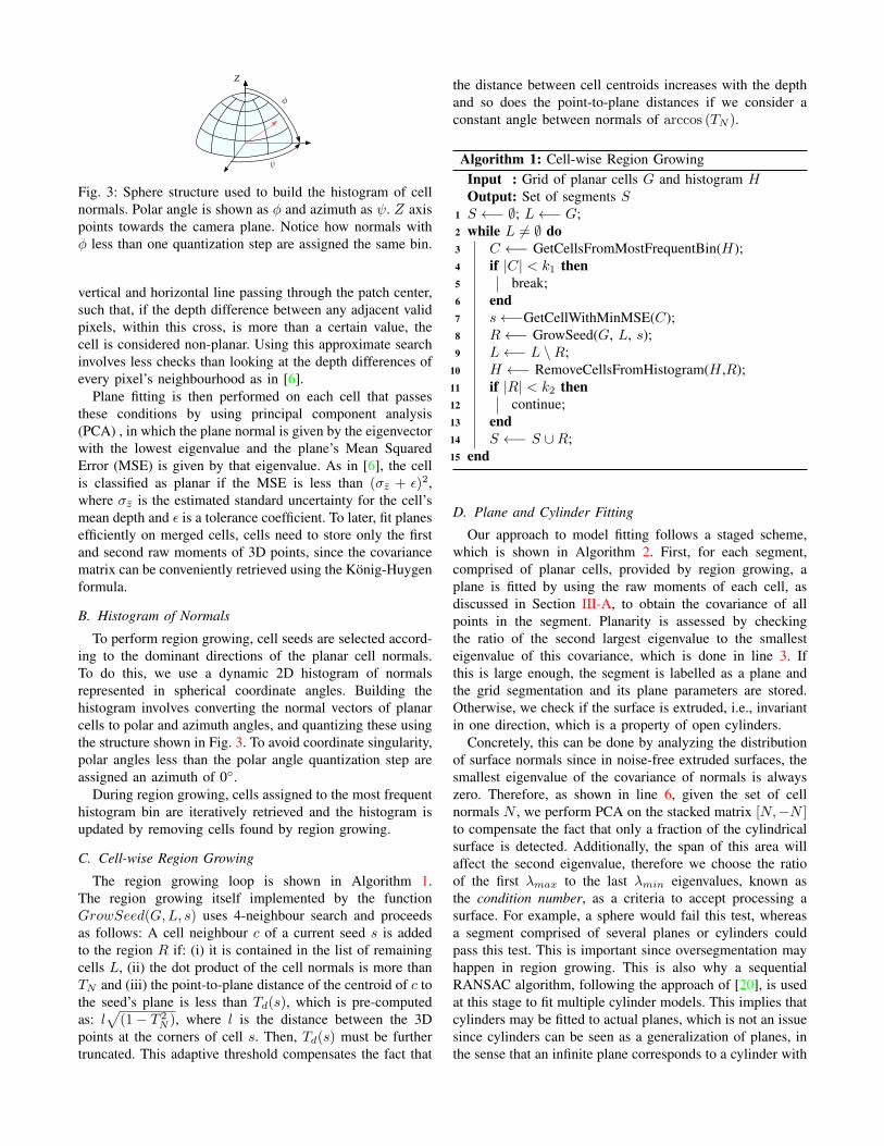
Fig. 3: Sphere structure used to build the histogram of cellnormals. Polar angle is shown as φ and azimuth as ψ. Z axispoints towards the camera plane. Notice how normals withφ less than one quantization step are assigned the same bin.

vertical and horizontal line passing through the patch center,such that, if the depth difference between any adjacent validpixels, within this cross, is more than a certain value, thecell is considered non-planar. Using this approximate searchinvolves less checks than looking at the depth differences ofevery pixel’s neighbourhood as in [6].

Plane fitting is then performed on each cell that passesthese conditions by using principal component analysis(PCA) , in which the plane normal is given by the eigenvectorwith the lowest eigenvalue and the plane’s Mean SquaredError (MSE) is given by that eigenvalue. As in [6], the cellis classified as planar if the MSE is less than (σz + ε)2,where σz is the estimated standard uncertainty for the cell’smean depth and ε is a tolerance coefficient. To later, fit planesefficiently on merged cells, cells need to store only the firstand second raw moments of 3D points, since the covariancematrix can be conveniently retrieved using the König-Huygenformula.

B. Histogram of Normals

To perform region growing, cell seeds are selected accord-ing to the dominant directions of the planar cell normals.To do this, we use a dynamic 2D histogram of normalsrepresented in spherical coordinate angles. Building thehistogram involves converting the normal vectors of planarcells to polar and azimuth angles, and quantizing these usingthe structure shown in Fig. 3. To avoid coordinate singularity,polar angles less than the polar angle quantization step areassigned an azimuth of 0◦.

During region growing, cells assigned to the most frequenthistogram bin are iteratively retrieved and the histogram isupdated by removing cells found by region growing.

C. Cell-wise Region Growing

The region growing loop is shown in Algorithm 1.The region growing itself implemented by the functionGrowSeed(G,L, s) uses 4-neighbour search and proceedsas follows: A cell neighbour c of a current seed s is addedto the region R if: (i) it is contained in the list of remainingcells L, (ii) the dot product of the cell normals is more thanTN and (iii) the point-to-plane distance of the centroid of c tothe seed’s plane is less than Td(s), which is pre-computedas: l

√(1− T 2

N ), where l is the distance between the 3Dpoints at the corners of cell s. Then, Td(s) must be furthertruncated. This adaptive threshold compensates the fact that

the distance between cell centroids increases with the depthand so does the point-to-plane distances if we consider aconstant angle between normals of arccos (TN ).

Algorithm 1: Cell-wise Region GrowingInput : Grid of planar cells G and histogram HOutput: Set of segments S

1 S ←− ∅; L←− G;2 while L 6= ∅ do3 C ←− GetCellsFromMostFrequentBin(H);4 if |C| < k1 then5 break;6 end7 s←−GetCellWithMinMSE(C);8 R←− GrowSeed(G, L, s);9 L←− L \R;

10 H ←− RemoveCellsFromHistogram(H ,R);11 if |R| < k2 then12 continue;13 end14 S ←− S ∪R;15 end

D. Plane and Cylinder Fitting

Our approach to model fitting follows a staged scheme,which is shown in Algorithm 2. First, for each segment,comprised of planar cells, provided by region growing, aplane is fitted by using the raw moments of each cell, asdiscussed in Section III-A, to obtain the covariance of allpoints in the segment. Planarity is assessed by checkingthe ratio of the second largest eigenvalue to the smallesteigenvalue of this covariance, which is done in line 3. Ifthis is large enough, the segment is labelled as a plane andthe grid segmentation and its plane parameters are stored.Otherwise, we check if the surface is extruded, i.e., invariantin one direction, which is a property of open cylinders.

Concretely, this can be done by analyzing the distributionof surface normals since in noise-free extruded surfaces, thesmallest eigenvalue of the covariance of normals is alwayszero. Therefore, as shown in line 6, given the set of cellnormals N , we perform PCA on the stacked matrix [N,−N ]to compensate the fact that only a fraction of the cylindricalsurface is detected. Additionally, the span of this area willaffect the second eigenvalue, therefore we choose the ratioof the first λmax to the last λmin eigenvalues, known asthe condition number, as a criteria to accept processing asurface. For example, a sphere would fail this test, whereasa segment comprised of several planes or cylinders couldpass this test. This is important since oversegmentation mayhappen in region growing. This is also why a sequentialRANSAC algorithm, following the approach of [20], is usedat this stage to fit multiple cylinder models. This implies thatcylinders may be fitted to actual planes, which is not an issuesince cylinders can be seen as a generalization of planes, inthe sense that an infinite plane corresponds to a cylinder with

Fig. 4: Direct cylinder fitting solution based on cell normalsfor a convex cylinder. First, cell centroids and normals areprojected onto a plane according to the cylinder axis. Second,an analytical circle fitting solution is used to estimate theradius and center.

infinite radius. After obtaining one or multiple subsegmentsof R from the RANSAC process, to find if they belong toeither planes or cylinders, a plane is fitted to each subsegmentand the respective MSE is compared against the MSE ofthe cylinder, which is given by point-to-axis distances. Interms of RANSAC implementation, each iteration selectsthree cells, although two is the minimal case, and uses thesolution explained below to find cylinder parameters.

Our proposed solution to cylinder fitting based on normalsis depicted in Fig. 4. It exploits the fact that surface nor-mals should intersect orthogonally the cylinder axis. Let thecolumn vectors Pi and Ni be respectively the centroid andthe plane normal of one cell among the n cells containedin a segment. Then, first, the cylinder axis v is foundthrough the PCA on the normal vectors described above,where v corresponds to the eigenvector with the smallesteigenvalue. To simplify the problem as a circle fitting one,the cell centroids and normals are projected on the planeperpendicular to v passing through the origin of the referenceframe. Concretely, a projected point is given by:

P ′i = Pi − v(v · Pi) (1)

whereas projected normals N ′ are obtained the same waybut then normalized. We can now cast the circle fitting as a1D linear least squares problem by minimizing:

E =

m∑i

(P ′i − rN ′i − C)2

2(2)

where C is the circle center and r is the radius. If we set thederivative of (2) wrt. r equal to zero, we arrive at the radiussolution:

r =(

1− 1

m

m∑i

N ′>i N ′)−1( 1

m

m∑i

N ′>i (P ′i − P ′))

(3)

where N ′ and P ′ represent the respective means. Then, giventhis estimated radius, the circle center is

C =1

m

m∑i

(P ′i − rN ′i) (4)

This solution is valid only when the normals point outwards.Otherwise, the radius is negative, thus we take its absolutevalue.

To apply this method to RANSAC, inliers are detected byusing the residual in (2) divided by the estimated radius,since (2) increases with the radius, given noisy normals.Inliers are selected if this relative error is less than 15%and the MSAC criteria [21] is used to score each modelhypothesis. We have tried alternatively using the point-to-circle distance but we found this was not as discriminative,as it fits a cylinder to several planar surfaces. Finally, themodel is refined with all the inliers in (3) and (4).

Algorithm 2: Plane and Cylinder fittingInput : Segment R and its cell normals N and

centroids POutput: Set of planes M and set of cylinders C

1 M←− ∅; C ←− ∅;2 plane_score ←− FitPlane(R);3 if plane_score > plane_min_score then4 M←−M∪R;5 else6 {v, λmax, λmin} ←− PCA(−N ∪N );7 if λmax/λmin > extrusion_min_score then8 {P ′, N ′} ←− ProjectToPlane(P,N, v);9 {I} ←− FitCylinderWithSeqRANSAC(P ′, N ′);

10 foreach subsegment Ii ∈ I do11 FitPlane(Ii);12 if MSEplane(Ii) ≤ MSEcylinder(Ii) then13 M←−M∪ Ii;14 else15 C ←− C ∪ Ii;16 end17 end18 end19 end

E. Model Segment Refinement

The grid segments seen in Fig. 2 are quite coarse, thus theirboundaries are refined. In PEAC, these are refined by usingpixel-wise region growing. Unfortunately, as revealed in thetiming results in [6], this step is computationally expensiveand moreover it does not guarantee accurate results, asshown in Fig 1, top-left image, as segments can growunbounded beyond their surface since pixel normals are notconsidered. Therefore, we propose a cell-bounded searchbased on morphological operations on the cell grid: First,each grid segment is eroded using a 3×3 kernel (searchingelement) to remove the boundary cells. This first step is alsoperformed by the refinement algorithm in [6]. In this work,we discard segments that are completely eroded, and use a 4-neighbour erosion kernel which is less destructive than the 8-neighbour kernel. Then, the original segment is dilated withan 8-neighbour 3×3 kernel to possibly expand our segment.The cells valid for refinement are given by the difference

CAPE

Depth Map

Probabilistic

Cylinder Fitting

Probabilistic

Plane Fitting

Cylinder

Matching

Plane

Matching

Pose Estimation

Depth Fusion

Fig. 5: Pipeline of VO in [5] extended by this work. Exten-sions are colored in red.

between the dilated segment and the eroded segment. Theseare shown as white cells in Fig. 2. The distance betweenthe segment model and each point within these cells iscalculated, so that each pixel is assigned to the model if itssquare distance is less than the model MSE times a constant(k = 9 in this work) and if it is the minimum distance toany model sharing the refinement cell. Thus, distances needto be stored while the segments are refined.

IV. CYLINDERS FOR RGB-D ODOMETRY

To exploit both the extracted planes and cylinder primitivesfor VO, we extended the RGB-D odometry frameworkmethod in [5] to cylinders. The original system alreadyallows the use of points, lines and plane features withina probabilistic framework that models and propagates theuncertainty of depth and the feature parameters. How-ever, contrary to full SLAM systems and sophisticated VOmethods, the pose estimation uses a basic frame-to-framescheme, which is known to be prone to drift. To addressthe sensor depth noise, the framework also incorporates aprobabilistic depth filter for spatio-temporal depth fusionbased on Mixture of Gaussians that models explicitly thedepth uncertainty. Fig. 5 highlights the extensions madeby this paper to this framework , while a more detailedmodel with points, line segments can be found at [5]. Afterextracting plane and cylinder segments and their parameters,probabilistic model fitting solutions are used to refine theparameters and derive their uncertainty, then cylinders andplanes are matched heuristically between last and currentframe and these matches are then aligned by a joint poseoptimization module based on iteratively reweighted leastsquares. Temporal depth fusion is then performed giventhe estimated pose, but unfortunately, as one can see inthis diagram, to exploit the benefits of depth fusion in thisframework, CAPE has to run twice per frame, pushing evenfurther the speed requirements of feature extraction. Thesenovel modules for cylinder primitives are detailed below.

A

B

Pi

Fig. 6: Iterative cylinder fitting solution. Planes represent thegauge constraint.

A. Probabilistic Cylinder Fitting

To refine the parameters of the final cylinder segmentsby taking into account the segment pixels (instead of cells)and their depth uncertainties, we propose here an iterativeprobabilistic cylinder fitting based on non-linear weightedleast squares, which is illustrated in Fig. 6.

Here, a cylinder is represented by two points along theaxis {A,B} and the radius r. For estimating these, a minimalparameterization is possible by fixing one dimension for thetwo points. These are initialized using the center and theaxis given by the solution in Section III-D, and then we fixthe 3D coordinate which has the largest range. As a result,the parameter vector has 5 dimensions in total, which areestimated by minimizing the sum of point to cylinder surfacedistances given by:

E =

m∑i

wi

(‖(B −A)× (A− Pi)‖‖B −A‖

− r)2

(5)

Ideally, the weights wi should be the inverse uncertaintyof the residuals, however for simplicity and efficiency inthis work we used the inverse of the depth uncertainties,as in [5]. The uncertainty of the parameters is then finallybackpropagated using the Hessian approximation:

Σξ = (J>r Σ−1r Jr)

−1 (6)

where Jr is the Jacobian matrix of the residuals wrt. theestimated parameters ξ, evaluated at the solution, and Σr is adiagonal matrix containing the uncertainties of the residuals,which are found by first order propagation of the 3D pointuncertainties through (5). It is worth noting that due to thecoordinate constraint, the obtained uncertainties for the twopoints are flat as shown in Fig. 6.

In practice, the number of points per segment is too high,thus we subsample these using a grid with step size of 5pixels. Although, significantly slower than the direct solutionin Section III-D, this solution takes around 4 iterationsto converge using analytical Jacobians and a Levenberg-Marquardt solver, whereas with numerical Jacobian compu-tation it takes around 50 iterations.

B. Cylinder Matching

For matching two cylinders between successive frames,we first check if the minimal angle formed by the two

cylinder axis is less than a specified threshold (30◦) and ifthe Mahalanobis distance between the radii: (r1−r2)2

σ2r1

+σ2r2

is lessthan a maximum value, heuristically set to 2000. The radiusuncertainties are extracted from (6). If a match passes theseconditions, we then check if their image segment overlapis more than half of the size of the smallest segment, asproposed in [5] for plane segments.

C. Pose Estimation based on Cylinders

To estimate the relative camera pose: {R, t | R ∈SO(3), t ∈ R3}, given a match between a cylinder with pointparameters {A,B} and a cylinder represented by {A′, B′},we express their error in the vector form as:

rc =

[(B −A)× (A−RA′ − t)(B −A)× (A−RB′ − t)

](7)

Effectively, this reflects the alignment between cylinder axes.For two plane matches with equations {N, d} and {N ′, d′},we make use of the plane-to-plane distance, described in [5],such that, the residual can be derived, in the vector form, as:

rp = N ′>R(N ′>t+ d′)− dN> (8)

Let the set of plane matches be P and the set of cylindermatches be C, then pose can be estimated by minimizing:

E = αplane

∑p∈P

rpWpr>p + αcylinder

∑c∈C

r>c Wcrc (9)

where αplane and αcylinder are two fixed scaling factors con-trolling the impact of the feature-types and Wp and Wc arediagonal weight matrices that are computed in every iterationas the inverse of the uncertainties of the residuals (7) and(8), which are obtained through first order error propagationof the feature parameter uncertainties, given by probabilisticmodel fitting, that is (6) for cylinders. For robustness, wecombine (9) with reprojection errors of points and lines asin [5].

V. EXPERIMENTS

We have conducted experiments on scenes with and with-out cylindrical surfaces. For non-cylindrical surfaces, weevaluate performance on a few sequences from the TUMRGB-D dataset [23] captured by structured-light Kinect andthe synthetic ICL-NUIM dataset [22], whereas to capturecylindrical surfaces, we have collected 3 sequences withan Occipital Structure sensor, shown in Fig. 7 and thesupplementary video (see Fig. 1). A markerboard was used tomeasure the pose ground truth. While the shorter yoga_matsequence contains ground truth for many frames, the othertwo only contain ground truth in the beginning and end ofthe trajectory as theses were captured in a close-loop. Timingresults for the feature extraction are reported in the SectionV-B and the performance of VO is evaluated in Section V-C

yoga mat spiral stairway tunnel

Fig. 7: Frames from the dataset collected in this work,processed by CAPE.

A. Implementation Details

All results were obtained on a PC with Intel i5-5257UCPU, using a single core. Depth maps were processed inVGA resolution. Both CAPE and PEAC were used with apatch size of 20×20 pixels. The remaining parameters forPEAC were left as default values, whereas CAPE parameterswere sensibly set to: TN = cos(π/12), plane_min_score =100, extrusion_min_score = 100, k1 = 5, k2 = 5 and thehistogram has 400 bins. In terms of VO, we used depth fusionwith a maximum sliding window of 5 frames and combinedfeature points with the features given by CAPE or PEAC,except where noted. The scaling factors in (9) are fine-tunedin Section V-C.

B. Processing Time

The feature extraction timings are shown in Fig. 8 for threesequences from three different datasets. CAPE performsconsistently across the sequences taking on average 3 ms andthe spiral_stairway sequence shows a negligible overheadintroduced by cylinder segments. By contrast, PEAC, besidesbeing 4-10 times slower on average, it exhibits a largevariance and a heavy-tail. Interestingly, PEAC is significantlyslower in the living room sequence and one can also see a bi-modal distribution. On close inspection, we observed that thelarge variances are due to the clustering and refinement stepsand that clustering gets slower when the camera faces closelyone wall, which increases the number of merging attemptsby the clustering algorithm. Following this observation, wetimed both CAPE and PEAC on a synthetic noise-free walland obtain respectively: 2.6 and 34 ms with a 20×20 patchand 5.8 and 300 ms with 10×10 patch.

C. Visual Odometry Performance

First, the trajectory estimation error of VO is summarizedin Fig. 9 for the yoga mat sequence while the impact ofplanes and cylinders on pose estimation, i.e., the feature-types weights in (9), are changed based on grid search.This is demonstrated as the absolute trajectory error (ATE)given the trajectory ground truth shown in Fig. 10. Settingall factors to zero means that the VO only uses pointfeatures. Up to αplane = 0.05, the performance of usingplanes extracted by PEAC is improved, but after that, theperformance is severely degraded. By the contrary, CAPEwith only planes fails to improve the performance as thisdiscards the cylinder surface. This suggests that it is betterto model this surface as a plane that not modelling at all.However, as we introduce cylinders extracted by CAPE,

Fig. 8: Timing results as violin plots for three sequences.The sequence desk corresponds to the fr1_desk of [23] andthe sequence living room corresponds to the lr kt0 in [22].

Fig. 9: Impact of the joint pose estimation residual weightson the ATE as RMSE in mm.

the error is consistently decreased for all plane weights,outperforming PEAC significantly. Based on Fig. 9 andperformance on other sequences, we fix αplane = 0.01 andαcylinder = 0.1 for the remaining experiments.

The trajectories estimated for the other two sequences areshown in Fig. 11 and the respective final errors are reportedin Table I. We have found that combining just feature pointswith the planes and cylinders performed poorly on theseenvironments as these are dominated by uniform surfaces,thus, here, we employed line segments as in the originalsystem. While using PEAC, degrades the performance of thebaseline, CAPE with cylinder primitives is able to improvethe performance particularly on the spiral_stairway, wherethe user walked up and down the same stairs, thus trajectoryshould be two closely aligned lines in Fig. 11.

Seq. (distance) Points &Lines

Points &Lines & PEAC

Points &Lines & CAPE

Tunnel (44 m) 2.3 m23 deg

4.9 m32 deg

1.8 m19 deg

Spiral stairway (51 m) 3.0 m6 deg

4.2 m25 deg

0.7 m6 deg

TABLE I: Final trajectory errors for the RGB-D sequencescollected in this work.

Results on cylinder-free scenes are reported in TableII. Although, performance is similar for several sequences,we can see in fr1_360 that PEAC can outperform CAPE.

0 5 10 15-1

0

1

P (

m)

x

x gt

0 5 10 15-1.0

-0.5

0

P (

m)

y

y gt

0 5 10 15

Time (s)

0

0.5

1.0

1.5

P (

m)

z

z gt

0 5 10 15-100

0

100

Angle

(deg

)

roll

roll gt

0 5 10 15-100

0

100

Ang

le (

deg

)

yaw

yaw gt

0 5 10 15

Time (s)

50

100

150

Ang

le (

deg

)

pitch

pitch gt

Fig. 10: Ground truth trajectory of the yoga_mat sequencealong with the path estimated by VO using CAPE.

-2 0 2 4 6 8 10

X (m)

-6

-4

-2

0

2

4

6

Y (

m)

Points + Lines

Points + Lines + PEAC

Points + Lines + CAPE

2

-5

1

-4

-2

-1

0

-3

Z (

m)

10 8 6X (m)4 2 0

Y (

m)

10

5

0

-5

X (m)5 0 -5 -10 -15 -20 -25

Points + Lines

Points + Lines + PEAC

Points + Lines + CAPE

Z (

m)

6

4

2

0

-25

-2

-20-15X (m)

-4

-10-50

-6

5

Points + Lines

Points + Lines + PEAC

Points + Lines + CAPE

Fig. 11: Trajectories estimated on two sequences: Top rowcorresponds to the spiral_stairway. Bottom row correspondsto the tunnel. Left column is the top view and right columnis a side view. End of the trajectories are marked by a circle.The black one is the ground truth final position.

We have noted that, with the specified parameters, PEACcan extract more planes far away from the camera thanthe selective CAPE, which can be advantageous for poseestimation when the number of features is critically low, asindicated by Fig. 9.

VI. CONCLUSIONS AND LIMITATIONS

We demonstrated a consistently fast plane and cylinderextraction method that improves VO performance on scenesmade of cylindrical surfaces. We believe this contributioncan be further beneficial for full SLAM and model trackingsystems. Operating on image cells instead of points, is keyfor efficiency and to deal with sensor noise, however thissacrifices resolution in the sense that surfaces smaller thanthe patch size are filtered out. Although this is not severein VO as we are more concerned about large stable surfaces

Seq. Points & PEAC Points & CAPEfr1_desk 62 mm / 25 mm / 1.8 deg 49 mm / 25 mm / 1.8 degfr1_360 117 mm / 68 mm / 3.3 deg 131 mm / 73 mm / 3.3 degfr3_struct_ntxt_far 80 mm / 36 mm / 0.9 deg 80 mm / 35 mm / 0.9 degor kt0 w/ noise 209 mm / 7 mm / 0.5 deg 160 mm / 7 mm / 0.5 deg

TABLE II: Performance on non-cylindrical scenes frompublic datasets, in terms of RMSE, shown in the followingorder: ATE / relative translational error / relative angularerror of trajectory.

than smaller objects, which can be captured using featurepoints, this can be an issue for robotic grasping applications.Thus the parameters used here need further fine-tuning forother applications. Yet a more promising idea is to implementa multi-scale search. Another limitation, is that segmentsgiven by region growing that form more complex shapes (i.e.not extruded), are also removed. Therefore, incorporatingother primitives such as spheres and cones remains as aworthwhile future direction.

REFERENCES[1] R. F. Salas-Moreno, B. Glocken, P. H. Kelly, and A. J. Davison,

“Dense planar slam,” in IEEE International Symposium on Mixed andAugmented Reality (ISMAR), pp. 157–164, 2014.

[2] Y. Taguchi, Y.-D. Jian, S. Ramalingam, and C. Feng, “Point-planeslam for hand-held 3d sensors,” in IEEE International Conference onRobotics and Automation (ICRA), pp. 5182–5189, 2013.

[3] M. Hsiao, E. Westman, G. Zhang, and M. Kaess, “Keyframe-baseddense planar slam,” in IEEE International Conference on Roboticsand Automation (ICRA), IEEE, 2017.

[4] L. Ma, C. Kerl, J. Stückler, and D. Cremers, “Cpa-slam: Consistentplane-model alignment for direct rgb-d slam,” in IEEE InternationalConference on Robotics and Automation (ICRA), pp. 1285–1291,IEEE, 2016.

[5] P. F. Proença and Y. Gao, “Probabilistic rgb-d odometry based onpoints, lines and planes under depth uncertainty,” Robotics and Au-tonomous Systems. In press, arXiv preprint: arXiv:1706.04034v3.

[6] C. Feng, Y. Taguchi, and V. R. Kamat, “Fast plane extraction inorganized point clouds using agglomerative hierarchical clustering,” inIEEE International Conference on Robotics and Automation (ICRA),pp. 6218–6225, 2014.

[7] D. Holz and S. Behnke, “Fast range image segmentation and smooth-ing using approximate surface reconstruction and region growing,” inIntelligent autonomous systems 12, pp. 61–73, Springer, 2013.

[8] A. J. Trevor, S. Gedikli, R. B. Rusu, and H. I. Christensen, “Efficientorganized point cloud segmentation with connected components,”Semantic Perception Mapping and Exploration (SPME), 2013.

[9] M. Y. Yang and W. Förstner, “Plane detection in point cloud data,” inProceedings of the 2nd int conf on machine control guidance, Bonn,vol. 1, pp. 95–104, 2010.

[10] J. Biswas and M. Veloso, “Depth camera based indoor mobile robotlocalization and navigation,” in IEEE International Conference onRobotics and Automation (ICRA), pp. 1697–1702, 2012.

[11] R. Schnabel, R. Wahl, and R. Klein, “Efficient ransac for point-cloudshape detection,” in Computer graphics forum, vol. 26, pp. 214–226,Wiley Online Library, 2007.

[12] G. Vosselman, B. G. Gorte, G. Sithole, and T. Rabbani, “Recognisingstructure in laser scanner point clouds,” International archives ofphotogrammetry, remote sensing and spatial information sciences,vol. 46, no. 8, pp. 33–38, 2004.

[13] T. Rabbani and F. Van Den Heuvel, “Efficient hough transform forautomatic detection of cylinders in point clouds,” ISPRS WG III/3,III/4, vol. 3, pp. 60–65, 2005.

[14] F. A. Limberger and M. M. Oliveira, “Real-time detection of planarregions in unorganized point clouds,” Pattern Recognition, vol. 48,no. 6, pp. 2043–2053, 2015.

[15] J. Poppinga, N. Vaskevicius, A. Birk, and K. Pathak, “Fast plane detec-tion and polygonalization in noisy 3d range images,” in InternationalConference on Intelligent Robots and Systems (IROS), pp. 3378–3383,IEEE, 2008.

[16] D. Holz, S. Holzer, R. B. Rusu, and S. Behnke, “Real-time planesegmentation using rgb-d cameras,” in Robot Soccer World Cup,pp. 306–317, Springer, 2011.

[17] R. F. Salas-Moreno, R. A. Newcombe, H. Strasdat, P. H. Kelly, andA. J. Davison, “Slam++: Simultaneous localisation and mapping at thelevel of objects,” in Computer Vision and Pattern Recognition (CVPR),2013 IEEE Conference on, pp. 1352–1359, IEEE, 2013.

[18] S. L. Bowman, N. Atanasov, K. Daniilidis, and G. J. Pappas, “Proba-bilistic data association for semantic slam,” in Robotics and Automa-tion (ICRA), 2017 IEEE International Conference on, pp. 1722–1729,IEEE, 2017.

[19] P. Hansen, H. Alismail, P. Rander, and B. Browning, “Pipe mappingwith monocular fisheye imagery,” in Intelligent Robots and Systems(IROS), 2013 IEEE/RSJ International Conference on, pp. 5180–5185,IEEE, 2013.

[20] M. Zuliani, C. S. Kenney, and B. Manjunath, “The multiransacalgorithm and its application to detect planar homographies,” in ImageProcessing, 2005. ICIP 2005. IEEE International Conference on,vol. 3, pp. III–153, IEEE, 2005.

[21] P. H. Torr and A. Zisserman, “Mlesac: A new robust estimator withapplication to estimating image geometry,” Computer vision and imageunderstanding, vol. 78, no. 1, pp. 138–156, 2000.

[22] A. Handa, T. Whelan, J. McDonald, and A. Davison, “A benchmarkfor RGB-D visual odometry, 3D reconstruction and SLAM,” in IEEEInternational Conference on Robotics and Automation (ICRA), IEEE,2014.

[23] J. Sturm, N. Engelhard, F. Endres, W. Burgard, and D. Cremers, “Abenchmark for the evaluation of rgb-d slam systems,” in InternationalConference on Intelligent Robots and Systems (IROS), IEEE, 2012.