fairness and redistribution - le
TRANSCRIPT

Fairness and redistribution
9 December 2007
Abstract
The median voter model (direct democracy) has wide applicability, but it is based
on sel�sh voters. i.e., voters who derive utility solely from �own�payo¤. A growing
and already large literature has pointed to fairness and concern for others as basic
human motivations that explain a range of economic phenomena. We examine the
implications of introducing fair voters who have a preference for fairness as in Fehr
and Schmidt (1999). Within a simple general equilibrium model, we demonstrate
the existence of a Condorcet winner for fair voters using the single-crossing property
of voters�preferences. In a fair-voter model, unlike a sel�sh-voter model, poverty
can lead to increased redistribution. Mean preserving spreads of income increase
equilibrium redistribution. Greater fairness leads to greater redistribution. An em-
pirical exercise using OECD data illustrates the potential importance of fairness in
explaining redistribution.
Keywords: Redistribution, other-regarding preferences, single-crossing property,
income inequality, American Exceptionalism.
JEL Classi�cation: D64 (Altruism); D72 (Economic Models of Political Processes:
Rent-Seeking, Elections, Legislatures, and Voting Behavior); D78 (Positive Analysis
of Policy-Making and Implementation).
1. Introduction
All societies face the issue of aggregating individual preferences into social outcomes. Inactual practice, such policies are chosen through the institution of representative democracyi.e. by the elected representatives of the citizens. Thus, the political process is complicatedby issues of political agency, information asymmetries, and legislative logrolling etc.; see,for instance, Persson and Tabellini (2000). However, in a range of applications in politicaleconomy, one often needs to abstract away from some of these issues. Indeed, there is a richliterature in public economics that relies on political choice through the institution of directdemocracy in which, a median voter directly chooses the social outcome. The pioneeringwork on redistribution within a direct democracy framework was done by Romer (1975),Roberts (1977), Meltzer and Richard (1981).1 The, commonly used, collective name forthis class of models is the �RRMR�model.Recent experience in Western democracies suggests that direct democracy is more than
a useful benchmark. Figures given in Matsusaka (2005a) (who terms the increasing trendin direct democracy as the �storm in ballot box lawmaking�) are instructive. In the US, 70percent of the population lives in a state or city where the apparatus of direct democracy isavailable. There have been at least 360 citizen initiated measures in the last 10 years in theUS and at least 29 referenda on monetary and market integration in Europe have alreadybeen held. Matsusaka (2005b) argues that there is a fundamental shift in how policydecisions are made. The implications of direct democracy for representative democracy areprofound2.
1.1. The RRMR model in brief
Since voters in the RRMR model care only about their narrow self-interest, we call it thesel�sh-voter model. In the basic model, the problem is to choose a linear progressive in-come tax rate that accomplishes redistribution in the sense that the post-tax distributionof income re�ects relatively greater equality. Romer (1975) laid out the conditions forsingle-peaked preferences when labor supply is endogenous. Roberts (1977) weakened the
1The existence of a Condorcet winner in a unidimensional policy space was �rst shown by Black (1948).2Direct citizen initiatives and referenda can override broken campaign promises and reduce the likeli-
hood that elected representatives choose policies that the majority will not desire. This mitigates agencyproblems to an extent. When information is dispersed among the electorate, a referendum can elicit suchinformation better, hence, direct democracy improves the quality of information. If legislatures bundlecontentious issues together, the possibility of referenda can force them to be unbundled. The same appliesto the attempts of politicians to bundle multiple issues. Thus, direct democracy induces greater trans-parency of issues. Limited information on the part of voters might not be a serious hindrance. Votersmight use information cues that permit a fairly informed decision. For instance, voters voting on theenvironment might just mimic the stance taken by Greenpeace or by Ralph Nader. For these and otherissues see Matsusaka (2005a).
1

single-peakedness condition to hierarchical-adherence. Gans and Smart (1996) proposedthe single-crossing property as an alternative method of determining a Condorcet win-ner and demonstrated that hierarchical adherence and single crossing are equivalent in aredistributive context.Meltzer and Richard (1981) derived the testable prediction that the extent of redis-
tribution directly depends on the ratio between mean and median income. The intuitionis that as inequality increases, the median voter is relatively poorer and, hence, choosesgreater redistribution.3 The evidence on the relation between inequality and redistributionis mixed, however. Positive support is found by Meltzer and Richard (1981), Easterly andRebelo (1993), Alesina and Rodrick (1994), Persson and Tabellini (1994), and Milanovic(2000). However, Lindert (1996), Perotti (1996) do not �nd any support.The RRMR framework treats only a speci�c kind of transfer, namely, the intra-
generational transfers of income. In actual practice, the growth of government transfersin recent decades has been driven by a range of other considerations. For instance, theincreased (inter-generational) transfers to the old could possibly re�ect their growing po-litical clout in Western democracies. Regional transfers could arise from special interestgroup considerations. Unemployment and health insurance can only be understood withinthe model insofar as these entail intra-generational transfers. These issues are possiblybetter analyzed within a dynamic model4.
1.2. Why fairness?
Traditional economic theory relies on the twin assumptions of rationality and self-interestedbehavior. The latter is generally taken to imply that individuals are interested primarilyin their own pecuniary payo¤s (sel�sh preferences). This view is not always in conformitywith the evidence. The purely sel�sh individual model is unable to explain a range ofphenomena frommany diverse areas such as collective action, contract theory, the structureof incentives, political economy and the results of several experimental games.Individuals are often found to be motivated by the pecuniary and non-pecuniary pay-
o¤s of others. A substantial fraction of individuals exhibit social preferences, i.e., theycare about the consumption and well being of others. Evidence from a range of experi-mental games, such as the ultimatum game, the gift exchange game, the public good gamewith punishment etc. can easily be reconciled if we assume individuals to have social
3It is not commonly realized that this follows from the special case of quasi-linear preferences withquadratic disutility from labour.
4Alesina and Rodrik (1994) discuss issues of growth and redistribution. Persson and Tabellini (1994)deal with a model of reputation in which the device of inter-generational punishment can sustain redis-tribution to the old. Tabellini (1991) shows how altruism among the young can sustain transfers to theold. Galasso and Conde Ruiz (2005) consider two policy tools: intra-generational and inter-generationaltransfers. Several models of unemployment insurance are surveyed in Persson and Tabellini (2000).
2

preferences.5
It may seem obvious to many that issues of fairness and regard for others (or socialpreferences) motivative the human desire to redistribute. The experimental results ofAckert et al. (2007), Tyran and Sausgruber (2006) and Bolton and Ockenfels (2002) arestrongly supportive of the importance of social preferences in the domain of voting models.Tyran and Sausgruber (2006) examine pure transfers of income from the rich to the poor
that do not a¤ect the middle income voter. Some rich voters, on account of their fairness,vote for transfers to the poor in circumstances where a rich, but sel�sh, voter would havevoted otherwise. Hence, a majority of the fair voters might vote for redistribution while,under identical circumstances, a sel�sh voter model would predict no redistribution.Bolton and Ockenfels (2002) examine the preference for equity versus e¢ ciency in a
voting game. Groups of three subjects are formed and are presented with two alternativepolicies: one that promotes equity while the other promotes e¢ ciency. The �nal outcomeis chosen by a majority vote. About twice as many experimental subjects preferred equityas compared to e¢ ciency. Furthermore, even those willing to change the status-quo fore¢ ciency are willing to pay, on average, less than half relative to those who wish to alterthe status-quo for equity.Our innovation is to replace the sel�sh voters in the RRMR sel�sh-voter model by fair
voters: this we will call the fair-voter model.
1.3. Which model of fairness?
There are several models of fairness. We choose to use the Fehr-Schmidt (1999) (hence-forth, FS) approach to fairness6. In this approach, voters care not only about their ownpayo¤s (as in the sel�sh voter model) but their payo¤s relative to those of others. Iftheir payo¤ is greater than other voters then they su¤er from advantageous inequity (aris-ing from, say, altruism) and if their payo¤ is lower than other voters they su¤er fromdisadvantageous inequity (arising from, say, envy).Several reasons motivate our choice of the FS model. The FS model is tractable and
explains the experimental results arising from several games where the prediction of thestandard game theory model with sel�sh agents yields results that are not consistent withthe experimental evidence. These games include the ultimatum game, the gift exchangegame, the dictator game as well as the public good game with punishment7.
5The references are too numerous to list here. A good place to start is the book by Camerer (2003)and the survey article by Fehr and Fischbacher (2002). The neuroeconomic foundations of reciprocity aresurveyed in Fehr et al. (2005).
6Bolton and Ockenfels (2000) provide yet another approach of inequity averse economic agents, but itcannot explain the outcome of the public good game with punishment, which is a fairly robust experimental�nding (see below).
7In the �rst three of these games, experimental subjects o¤er more to the other party relative to the
3

The FS model focusses on the role of inequity aversion. However, a possible objectionis that it ignores the role played by intentions that have been shown to be important inexperimental results (Falk et al. (2002)) and treated explicitly in theoretical work (Rabin(1993), Falk and Fischbacher (2006)). However, experimental results on the importanceof intentions come largely from bilateral interactions. Economy-wide voting, on the otherhand, is impersonal and anonymous, thereby ruling out any important role for intentions.Tyran and Sausgruber (2006) explicitly test for the importance of the FS framework
in the context of direct voting. They conclude that the FS model predicts much betterthan the standard sel�sh voter model. In addition, the FS model provides, in their words,�strikingly accurate predictions for individual voting in all three income classes.� Theeconometric results of Ackert et al. (2007), based on their experimental data, lend furthersupport to the FS model in the context of redistributive taxation. The estimated coe¢ -cients of altruism and envy in the FS model are statistically signi�cant and, as expected,negative in sign. Social preferences are found to in�uence participant�s vote over alter-native taxes. They �nd evidence that some participants are willing to reduce their ownpayo¤s in order to support taxes that reduce advantageous or disadvantageous inequity.
1.4. A critique of the literature on voting and fairness
There is a relatively small theoretical literature that considers fair voters. We concen-trate below on the papers that are directly relevant to our work. Tyran and Sausgruber(2006), reviewed above, do not analyze the relation between inequality and redistributivetaxes which is important in the RRMR framework (and ours�). Their�s is not a generalequilibrium model, does not analyze the e¢ ciency costs of redistribution and, probablymost importantly, does not provide existence results for there to be a decisive medianvoter. Furthermore, they consider a more restricted tax policy choice than us. While weconsider changes in a linear progressive income tax that a¤ect all taxpayers they focusattention only on redistributions from the rich to the poor that leave the middle incomevoters una¤ected8.Galasso (2003) modi�es the RRMR model to allow for fairness concerns. However,
his notion of fairness is not only one-sided but it is of a very speci�c form; it is notfully consistent with any of the accepted models of fairness. In particular, he assumesthat fair voters su¤er disutility through a term that is linear in their payo¤s relative to
predictions of the Nash outcome. In the public good game with punishment, the possibility of ex-postpunishment dramatically reduces the extent of free riding in voluntary giving towards a public good. Inthe standard theory with sel�sh agents, bygones are bygones, so there is no ex-post incentive for thecontributors to punish the free-riders. Foreseeing this outcome, free riders are not deterred, which is indisagreement with the evidence. Such behavior can be easily explained within the FS framework.
8They do introduce a cost of such redistribution to the middle income voters, but it is not an integralpart of the redistributive �scal package considered.
4

the worse o¤ voter in society.9 Since this concern for fairness arises from a linear term,preferences continue to be strictly concave and a median voter equilibrium exits. Withinthis framework there is greater redistribution when there is a mean preserving spread ininequality. However, this leaves open the question of whether a median voter equilibriumwill exist in a standard model of fairness, such as the FS model, and what the propertiesof the resulting equilibrium will be?
1.5. European versus American redistribution: A Case Study
Europe, where (disposable income) inequality is lower, undertakes greater redistributionthan America, where such inequality is higher. This would seem to contradict the RRMRmodel. Alesina and Angeletos (2003) have a novel explanation. The key to understandingtheir model is the individual beliefs on the source of poverty (or a uence). It is claimedthat more Americans than Europeans believe that poverty (or a uence) is caused byindividual e¤ort than luck. A crucial assumption of the model is that voters expect thereto be greater public redistribution if income outcomes are governed by luck rather thane¤ort. Hence, in the European equilibrium, more people believe that income is causedby luck, so put in less e¤ort and, hence, actual outcomes are indeed governed more byluck rather than e¤ort. Given the assumption on public redistribution, there is greaterredistribution in equilibrium. The American, high e¤ort - low redistribution equilibriumcan be understood analogously.Benabou (2000) develops a stochastic growth model with incomplete asset markets
and heterogeneous agents who vote over redistributive policies. He shows that multipleequilibria can exist, some featuring low inequality and high redistribution, while othersexhibit high inequality and low redistribution. Thus countries with similar preferences,technologies and political systems can feature very di¤erent levels of inequality and redis-tribution.Economic theory is very explicit about the inequality variable required: it should be
pre-tax/transfer distribution of income i.e. the factor income distribution. Theory doesnot necessarily predict any relation between disposable income distribution and the extentof redistribution. However, despite this important restriction, most empirical work on therelation between inequality and redistribution uses disposable income data. Factor incomedata has recently been made available in Milanovic (2000). The results in Milanovic (2000)
9The latter term captures some notion of social justice. Others have included such a term to incorporatesocial justice e.g. Charness and Rabin (2002). However, they posit preferences, di¤erent from Galasso(2003), that are a convex combination of the total payo¤ of the group (this subsumes sel�shness, in sofar as one�s own payo¤ is part of the total, and altruism) and a Rawlsian social welfare function. Thesesorts of models are able to explain positive levels of giving in dictator games, and reciprocity in trust andgift exchange games. However, they are not able to explain situations where an individual tries to punishothers in the group at some personal cost, for instance, punishment in public good games.
5

1
FII
920.6Swe/US
MultiAid/GDPSS/GDPDII
1
FII
920.6Swe/US
MultiAid/GDPSS/GDPDII
Figure 1.1: An illustrative comparison beween Sweden and the US
show that almost a third of factor income inequality is removed by government tax andtransfer programs. As an illustrative example, consider a relative comparison of Swedenand the US in Figure 1.1. DII denotes disposable income inequality, SS/GDP denotes theratio of social spending to gross domestic product, FII denotes factor income inequalityand Multi-Aid/GDP is multilateral aid to the GDP ratio. Swe/US gives the Swedish toUS ratio for the relevant variables.Disposable income inequality in Sweden is about 60 percent that of the US. The Swedish
social spending to GDP ratio is about twice that of the US. This raises the followingproblems for the classical theory which posits that �greater inequality creates greaterredistribution�; see for instance Meltzer and Richard (1981).
1. If one uses disposable income inequality (DII), which is the norm in applied work,then the US should undertake greater redistribution that Sweden, but we observethe exact opposite.
2. What if we were to use the variable suggested by theory i.e. factor income inequality?Factor income inequality (FII) is almost identical in the two countries. Theory wouldthen predict identical redistribution, which is not the case.
We provide an alternative explanation for greater European redistribution relative toAmerica by using the argument that Europeans are relatively more inequity averse (or fairin the Fehr-Schmidt sense) on average and that there is basis for �American Exceptional-ism�10. Measuring fairness presents a challenging, and understandably contentious, set ofissues. We now turn to these.One could possibly use charitable giving per capita as an indicator of fairness. How-
ever, charitable contributions are endogenous in a model with fair voters. So, for instance,if government redistribution is perceived to be inadequate, citizens might attempt to com-pensate by donating more to charity. For that reason we do not believe that the relatively
10A good summary of American Exceptionalism is provided in Glaeser (2005); the reasons includeproportional versus majoritarian representation, greater ethnic heterogeneity in America, and the UStradition of federalism that gives redistributive powers to the individual States, among others.
6

greater per capita giving of Americans necessarily indicates that they are more inequityaverse than Europeans.A better measure of fairness/inequity aversion seems to be �aid given to other countries�,
particularly, developing countries. As in the case of charitable contributions, aid given by acountry to any particular developing country could well re�ect the low volume of aggregategiving to that country in the �rst place. However, crucially, this applies equally to all givingcountries. Hence, relative giving of countries potentially re�ects relative fairness/ inequityaversion. This is the measure that we will use. We will use those measures of aid thatremove the e¤ects of strategic political considerations and other such confounding factors.The US is the single largest contributor to development aid. However, in per capita
terms its contribution is lower than most European countries. According to OECD �gures,the US contributed only 0.15 percent of its GDP to development assistance, placing it lastin a list of 21 western (mostly European) countries. The Center for Global Developmentestimated that US development assistance per capita is one eighth that of Norway, onesixth that of Denmark and close to half of the average contributions of Belgium, France,Finland and Britain.In terms of our Swedish versus US comparison in Figure 1.1, our proxy for inequity
aversion, multilateral aid to GDP ratio (this corrects for strategic giving), for Swedenis about 9 times that of the US. We argue that this reveals greater inequity aversionof the Swedes relative to the US and potentially helps to explain the di¤erences in thesocial spending to GDP ratios between the two countries; a di¤erence that factor incomeinequality is unable to explain.
1.6. Results and plan of the paper
Our main theoretical results are as follows. First, we demonstrate the existence of a Con-dorcet winner for voters who have the FS preferences for fairness. Insofar as one believesthat issue of fairness and concern for others underpin the human tendency to redistribute,this result opens the way for modelling such concerns in the context of direct democracy.Second, we �nd that if voters are fair, then increased poverty can lead to increased redis-tribution and the ratio of social spending to GDP would move countercyclically, which isat variance with the sel�sh voter model, but in agreement with the evidence.Due to the paucity of data on factor incomes, we claim to provide no more than an
illustrative empirical exercise that provides empirical support to the idea that fairness isan important determinant of redistribution. Conditional on the limitations of our exercise,our regression results, based on data from 20 OECD economies, can be summarized as fol-lows. First, factor income inequality leads to a better speci�cation than disposable incomeinequality. Second, the results support the idea of �American Exceptionalism�relative to
7

Europe. Third, our fairness variable is a signi�cant determinant of redistribution, whileincome inequality is not signi�cant.The plan of the paper is as follows. Section 2 describes the theoretical model and derives
some preliminary results. Section 3 establishes the existence of a Condorcet winner for fairvoters. Comparative static results along with some calibration exercises are derived anddiscussed in Section 4. Section 5 considers the relationship between income distributionand the tax rate using a discrete analogue of second order stochastic dominance. Section6 presents our illustrative empirical exercise. Finally, section 7 concludes. The results ofregression analysis are presented in Appendix 1. Proofs are relegated to Appendix 2.
2. Model
We consider a general equilibrium model as in Meltzer and Richard (1981). Let there ben = 2m � 1 � 3 voters, where m is the median voter. Let the skill level of voter i be si,where
0 < si < sj < 1, for i < j, (2.1)
and s = (s1; s2; :::; sn). Each voter has a �xed time endowment of one unit and supplies liunits of labor and so enjoys Li = 1� li units of leisure, where
0 � li � 1. (2.2)
Labour markets are competitive and each �rm has access to a linear production technol-ogy such that production equals sili. Hence, the wage rate o¤ered to each worker-votercoincides with the marginal product, i.e., the skill level, si. Thus, the before-tax incomeof a voter is given by
yi = sili. (2.3)
Note that �skill�here need not represent any intrinsic talent, just ability to translate laboure¤ort into income11. Let the average before-tax income be
y =1
n�ni=1yi. (2.4)
We make the empirically plausible assumption that the income of the median voter, ym,is less than the average income,
ym < y. (2.5)
11For example, a highly talented classical musician may be able to earn only a modest income, whilea merely competent �pop�musician may earn millions. In our model, the former would be classi�ed ashaving a low s while the latter would be classi�ed as having a high s. Similarly, in recent years, therehas been a record level of skilled (in the ordinary sense of the word) migration into Britain from EasternEurope. However, since they are predominantly accepting low pay work, they would be classi�ed in ourmodel as having low s.
8

The government operates a linear progressive income tax that is characterized by aconstant marginal tax rate, t,
t 2 [0; 1] , (2.6)
and a uniform transfer, b, to each voter that equals the average tax proceeds,
b = ty =t
n�ni=1yi =
t
n�ni=1sili � 0. (2.7)
Thus, the tax rate is also the ratio of social spending to aggregate income,
t =nb
�ni=1yi. (2.8)
Remark 1 : From (2.8), changes in the tax rate can equivalently be viewed as changesin the ratio of social spending to aggregate income.
The budget constraint of voter i is given by
0 � ci � (1� t) yi + b. (2.9)
In view of (2.3), the budget constraint (2.9) can be written as
0 � ci � (1� t) sili + b. (2.10)
2.1. Preferences, labour supply and indirect utility of a sel�sh voter
Voter i (whether sel�sh or fair) has a utility function, u(ci; 1� li), over own consumption,ci, and own leisure, 1� li. In common with the literature, we assume that all voters havethe same utility function. Hence, voters di¤er only in that they are endowed with di¤erentskill levels, si. We assume that the utility function is quasi-linear, with constant elasticityof labour supply, which is the most commonly used functional form in various applicationsof the median voter theorems.
u(c; 1� l) = c� �
1 + �l1+�� , (2.11)
where � is a constant satisfying0 < � � 1. (2.12)
The case � = 1 has special signi�cance in the literature. In this case,
u(c; 1� l) = c� 12l2 (2.13)
Meltzer and Richard (1981) use (2.13) to derive the celebrated result that the extent ofredistribution varies directly with the ratio of the mean to median income. Piketty (1995)
9
restricts preferences to the quasi-linear case with disutility of labour given by the quadraticform, (2.13). Benabou and Ok (2001) do not actually consider a production side and theirmodel has exogenously given endowments which evolve stochastically. Benabou (2000)considers the additively separable case with log consumption and disutility of labor givenby the constant elasticity case, (2.11).Since @u
@ci> 0, the budget constraint (2.10) holds with equality. Substituting ci =
(1� t) sili + b in the utility function of voter i, we get
U (li; t; b; si) = (1� t) sili + b��
1 + �l1+��
i . (2.14)
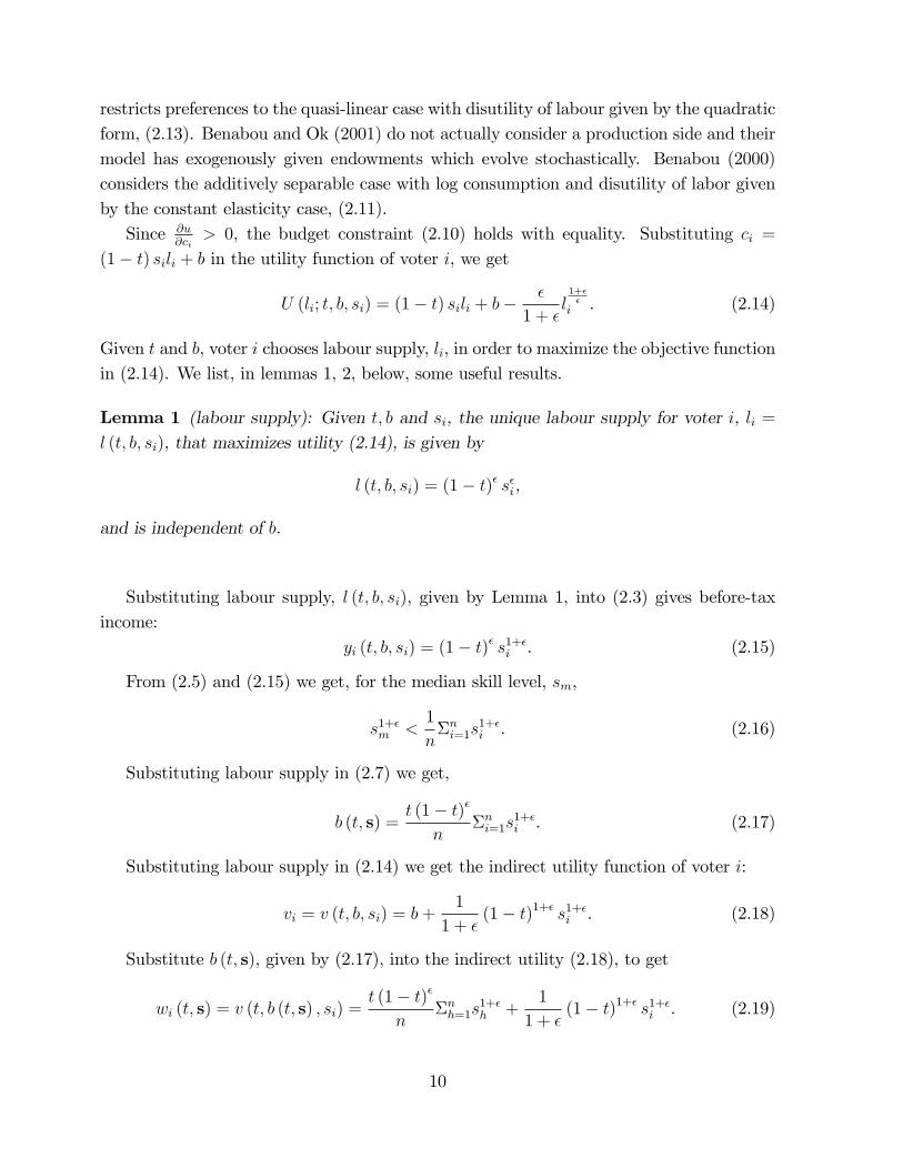
Given t and b, voter i chooses labour supply, li, in order to maximize the objective functionin (2.14). We list, in lemmas 1, 2, below, some useful results.
Lemma 1 (labour supply): Given t; b and si, the unique labour supply for voter i, li =l (t; b; si), that maximizes utility (2.14), is given by
l (t; b; si) = (1� t)� s�i ,
and is independent of b.
Substituting labour supply, l (t; b; si), given by Lemma 1, into (2.3) gives before-taxincome:
yi (t; b; si) = (1� t)� s1+�i . (2.15)
From (2.5) and (2.15) we get, for the median skill level, sm,
s1+�m <1
n�ni=1s
1+�i . (2.16)
Substituting labour supply in (2.7) we get,
b (t; s) =t (1� t)�
n�ni=1s
1+�i . (2.17)
Substituting labour supply in (2.14) we get the indirect utility function of voter i:
vi = v (t; b; si) = b+1
1 + �(1� t)1+� s1+�i . (2.18)
Substitute b (t; s), given by (2.17), into the indirect utility (2.18), to get
wi (t; s) = v (t; b (t; s) ; si) =t (1� t)�
n�nh=1s
1+�h +
1
1 + �(1� t)1+� s1+�i . (2.19)
10

Lemma 2 (properties of the indirect utility function): (a) @v@b= 1,
(b) @v@s= (1� t)1+� s�. Hence,
�@v@s
�t=1= 0 and t 2 [0; 1)) @v
@s> 0,
(c) @v@t= � (1� t)� s1+�. Hence,
�@v@t
�t=1= 0 and t 2 [0; 1)) @v
@t< 0,
(d) @@s
�@v@b
�= 0,
(e) @@s
�@v@t
�= � (1 + �) (1� t)� s�. Hence,
�@@s
�@v@t
��t=1= 0 and t 2 [0; 1)) @
@s
�@v@t
�< 0.
From Lemma 2(a), @v@b> 0. Thus, we can interpret @
@s
�@v@b
�� 0 as saying that the
marginal utility of an extra pound of bene�t for a rich person is never greater than thatfor a poor person. From Lemma 2(c), t 2 [0; 1) ) @v
@t< 0. Hence, @
@s
�@v@t
�< 0 can be
interpreted as saying that an extra 1% on the tax rate hurts a rich person more than apoor person. Thus, roughly speaking, bene�ts help the poor more than the rich whiletaxes hurt the rich more than the poor. This is the basic foundation of the modern welfarestate.
2.2. Preferences of fair voters
Fair voters have other-regarding preferences as in Fehr-Schmidt (1999). These preferencesare as follows
Vj (t; b; �; �; s) = v (t; b; sj)��
n� 1Pk 6=jmax f0; v (t; b; sk)� v (t; b; sj)g (2.20)
� �
n� 1Pi6=jmax f0; v (t; b; sj)� v (t; b; si)g ,
wherefor sel�sh voters � = � = 0, (2.21)
for fair voters 0 < � < 1; � < �. (2.22)
From (2.20), the fair voter cares about own payo¤(�rst term), payo¤relative to those whereinequality is disadvantageous (second term) and payo¤ relative to those where inequalityis advantageous (third term). The second and third terms which capture respectively, envyand altruism, are normalized by the term n � 1 where n is the number of voters. Noticethat in FS preferences, inequality is self-centered, i.e., the individual uses her own payo¤asa reference point with which everyone else is compared to. Also, while the Fehr-Schmidtspeci�cation is directly in terms of monetary payo¤s, it is also consistent with comparisonof payo¤s in utility terms. These and related issues are more fully discussed in Fehr andSchmidt (1999). From (2.22), � is bounded below by 0 and above by 1 and �. On theother hand, there is no upper bound on �.12
12� � 1 would imply that individuals could increase utility by simply giving away all their wealth; thisis counterfactual. The restriction � < � is based on experimental evidence. Finally the lack of an upperlimit on � implies that �envy�is unbounded.
11

In the light of Lemma 2(b), (2.20) becomes
Vj = v (t; b; sj)��
n� 1Pk>j
[v (t; b; sk)� v (t; b; sj)]��
n� 1Pi<j
[v (t; b; sj)� v (t; b; si)] ,
(2.23)or, equivalently,
Vj =�
n� 1Pi<j
v (t; b; si) +
�1� (j � 1) �
n� 1 +(n� j)�n� 1
�v (t; b; sj)�
�
n� 1Pk>j
v (t; b; sk) .
(2.24)Let
Wj (t; �; �; s) = Vj (t; b (t; s) ; �; �; s) ; (2.25)
where b (t; s) is given by (2.17). Then (2.19), (2.23), (2.24) and (2.25) give
Wj = wj (t; s)��
n� 1Pk>j
[wk (t; s)� wj (t; s)]��
n� 1Pi<j
[wj (t; s)� wi (t; s)] . (2.26)
and, equivalently,
Wj =�
n� 1Pi<j
wi (t; s) +
�1� (j � 1) �
n� 1 +(n� j)�n� 1
�wj (t; s)�
�
n� 1Pk>j
wk (t; s) .
(2.27)
Lemma 3 (Existence of a maximum): Given �; � and s,Wj (t; �; �; s) attains a maximumat some tj 2 [0; 1].
Remark 2 (Weighted utilitarian preferences): Note that the preferences of the fair voterin (2.27) can be rewritten in the following weighted utilitarian form
Wj (t; �; �; s) =nPi=1
!ijwi (t; s) , (2.28)
where
i < j ) !ij =�
n� 1 > 0, !jj = 1�(j � 1) �n� 1 +
(n� j)�n� 1 > 0, i > j ) !ij = �
�
n� 1 < 0,nPi=1
!ij = 1: (2.29)
12

2.3. Sequence of moves
We consider a two-stage game. In the �rst stage, voters choose a tax rate, t, anticipatingthe outcome of the second stage. Consumer j exhibits fairness by voting for the tax rate,
t, that would maximize social welfare,Wj (t; �; �; s) =nPi=1
!ijwi (t; s), as seen from her own
perspective (see Remark 2). In the second stage, consumer j chooses own labour supply,lj, so as to sel�shly maximize own utility, U (lj; t; b; sj), given t; b; sj. This determineslabour supplies, li = l (t; b; si), and indirect utilities, vi = v (t; b; si) = U (l (t; b; si) ; t; b; si),i = 1; 2; :::; n.
Remark 3 : One might wonder, why should the consumer not exhibit fairness in thesecond stage (when choosing own labour supply) as well as the �rst stage (when choosingthe tax rate)? However, it would make no di¤erence. To see this, suppose that in the second
stage consumer j chooses lj so as to maximizenPi=1
!ijU (li; t; b; si) = !jjU (lj; t; b; sj) +
nPi6=j!ijU (li; t; b; si) given t; b; sj and given si, li for all i 6= j. Then, since in the Fehr-Schmidt
theory, U (li; t; b; si), i 6= j, enter additively, and !jj > 0, it follows that maximizingnPi=1
!ijU (li; t; b; si) is equivalent to maximizing U (lj; t; b; sj).
3. Existence of a Condorcet winner
We now ask if a median voter equilibrium exists in a model with fair voters? As expected,single-peakedness of preferences turns out to be a very strong restriction. We instead usethe single-crossing property of Gans and Smart (1996).
De�nition 1 : (Gans and Smart, 1996) The �single-crossing�property holds if for taxrates t; T and voters j; J ,t < T , j < J , Wj (t; �; �; s) > Wj (T; �; �; s)) WJ (t; �; �; s) > WJ (T; �; �; s).13
Lemma 4 : (Gans and Smart, 1996) The �single-crossing�property holds if �@Vj@t=@Vj@bis
an increasing function of j.
Lemma 5 : (Gans and Smart, 1996) If the �single-crossing� property holds, then themedian voter is decisive, i.e., a majority chooses the tax rate that is optimal for themedian voter.13Here we use �<�to denote the usual ordering of real numbers. In the more general setting of Gans
and Smart (1996), �<�is used to denote several (possibly di¤erent) abstract orderings. In particular, aliteral translation of Gants and Smart (1996) would give: T < t, j < J , Wj (t; �; �; s) > Wj (T; �; �; s))WJ (t; �; �; s) > WJ (T; �; �; s), where �j < J �has the usual meaning �j is less than J �but �T < t �means �t is less than T �.
13

B
b'B
ptrtt
rI
rI
pI
pI
Figure 3.1: Illustration of the Gans-Smart single crossing property.
The proofs of lemmas 4, 5 can be found in Gans and Smart (1996). The intuition behindthese lemmas is straightforward to illustrate in the following diagram in (b; t) space. InFigure 3.1, the aggregate budget constraint of the economy, given in (2.7), is shown bythe straight upward sloping line, BB0, that has slope y. We show two indi¤erence curvesbelonging to a poor (IpIp) and a rich (IrIr) voter respectively. Lemma 4 requires that�@Vj
@t=@Vj@bbe an increasing function of j i.e. IpIp is relatively �atter (we show this in
section 3.1 below). The most preferred tax rate of the poor, tp, is greater than the mostpreferred tax rate of the rich, tr. Hence, the preferred tax rates can be uniquely orderedfrom the rich to the poor. This monotonicity property gives rise to the result in Lemma5.
3.1. Existence of a Condorcet winner
Proposition 1 : A majority prefers the tax rate that is optimal for the median-voter.
In light of the emerging evidence, it increasingly appears that issues of fairness and con-cern for others are important human motivations that play a signi�cant part in the actualdesign of redistributive tax policies. Insofar as actual applications of a direct democracyframework largely use quasi-linear preferences and constant elasticity of labour supply,Proposition 1 establishes the existence of a Condorcet winner. Hence, the result in Propo-sition 1 is potentially of fundamental importance for political economy models that seek
14
to incorporate social preferences.
4. Comparative static results
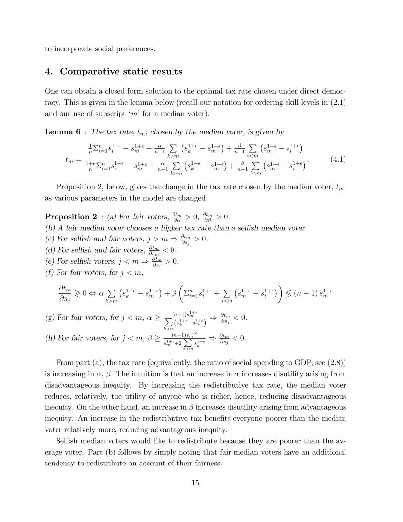
One can obtain a closed form solution to the optimal tax rate chosen under direct democ-racy. This is given in the lemma below (recall our notation for ordering skill levels in (2.1)and our use of subscript �m�for a median voter).
Lemma 6 : The tax rate, tm, chosen by the median voter, is given by
tm =
1n�ni=1s
1+�i � s1+�m + �
n�1Pk>m
�s1+�k � s1+�m
�+ �
n�1Pi<m
�s1+�m � s1+�i
�1+�n�ni=1s
1+�i � s1+�m + �
n�1Pk>m
�s1+�k � s1+�m
�+ �
n�1Pi<m
�s1+�m � s1+�i
� . (4.1)
Proposition 2, below, gives the change in the tax rate chosen by the median voter, tm,as various parameters in the model are changed.
Proposition 2 : (a) For fair voters, @tm@�> 0, @tm
@�> 0.
(b) A fair median voter chooses a higher tax rate than a sel�sh median voter.(c) For sel�sh and fair voters, j > m) @tm
@sj> 0.
(d) For sel�sh and fair voters, @tm@sm
< 0.(e) For sel�sh voters, j < m) @tm
@sj> 0.
(f) For fair voters, for j < m,
@tm@sj
? 0, �Pk>m
�s1+�k � s1+�m
�+ �
��ni=1s
1+�i +
Pi<m
�s1+�m � s1+�i
��7 (n� 1) s1+�m
(g) For fair voters, for j < m, � � (n�1)s1+�mPk>m(s1+�k �s1+�m )
) @tm@sj
< 0.
(h) For fair voters, for j < m, � � (n�1)s1+�m
s1+�m +2Pk>m
s1+�k
) @tm@sj
< 0.
From part (a), the tax rate (equivalently, the ratio of social spending to GDP, see (2.8))is increasing in �, �. The intuition is that an increase in � increases disutility arising fromdisadvantageous inequity. By increasing the redistributive tax rate, the median voterreduces, relatively, the utility of anyone who is richer, hence, reducing disadvantageousinequity. On the other hand, an increase in � increases disutility arising from advantageousinequity. An increase in the redistributive tax bene�ts everyone poorer than the medianvoter relatively more, reducing advantageous inequity.Sel�sh median voters would like to redistribute because they are poorer than the av-
erage voter. Part (b) follows by simply noting that fair median voters have an additionaltendency to redistribute on account of their fairness.
15
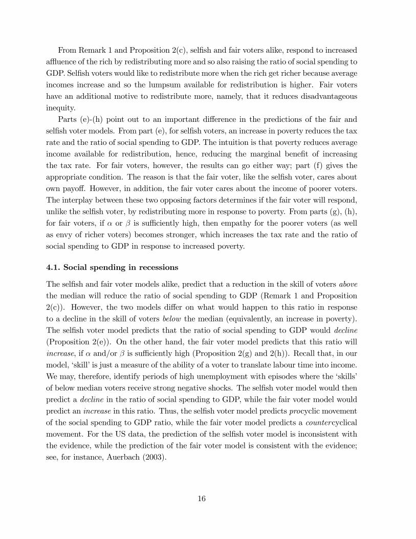
From Remark 1 and Proposition 2(c), sel�sh and fair voters alike, respond to increaseda uence of the rich by redistributing more and so also raising the ratio of social spending toGDP. Sel�sh voters would like to redistribute more when the rich get richer because averageincomes increase and so the lumpsum available for redistribution is higher. Fair votershave an additional motive to redistribute more, namely, that it reduces disadvantageousinequity.Parts (e)-(h) point out to an important di¤erence in the predictions of the fair and
sel�sh voter models. From part (e), for sel�sh voters, an increase in poverty reduces the taxrate and the ratio of social spending to GDP. The intuition is that poverty reduces averageincome available for redistribution, hence, reducing the marginal bene�t of increasingthe tax rate. For fair voters, however, the results can go either way; part (f) gives theappropriate condition. The reason is that the fair voter, like the sel�sh voter, cares aboutown payo¤. However, in addition, the fair voter cares about the income of poorer voters.The interplay between these two opposing factors determines if the fair voter will respond,unlike the sel�sh voter, by redistributing more in response to poverty. From parts (g), (h),for fair voters, if � or � is su¢ ciently high, then empathy for the poorer voters (as wellas envy of richer voters) becomes stronger, which increases the tax rate and the ratio ofsocial spending to GDP in response to increased poverty.
4.1. Social spending in recessions
The sel�sh and fair voter models alike, predict that a reduction in the skill of voters abovethe median will reduce the ratio of social spending to GDP (Remark 1 and Proposition2(c)). However, the two models di¤er on what would happen to this ratio in responseto a decline in the skill of voters below the median (equivalently, an increase in poverty).The sel�sh voter model predicts that the ratio of social spending to GDP would decline(Proposition 2(e)). On the other hand, the fair voter model predicts that this ratio willincrease, if � and/or � is su¢ ciently high (Proposition 2(g) and 2(h)). Recall that, in ourmodel, �skill�is just a measure of the ability of a voter to translate labour time into income.We may, therefore, identify periods of high unemployment with episodes where the �skills�of below median voters receive strong negative shocks. The sel�sh voter model would thenpredict a decline in the ratio of social spending to GDP, while the fair voter model wouldpredict an increase in this ratio. Thus, the sel�sh voter model predicts procyclic movementof the social spending to GDP ratio, while the fair voter model predicts a countercyclicalmovement. For the US data, the prediction of the sel�sh voter model is inconsistent withthe evidence, while the prediction of the fair voter model is consistent with the evidence;see, for instance, Auerbach (2003).
16

5. Income distribution and the tax rate
In section 4 we have already seen the redistributive e¤ect of changes in skill levels of votersabove and below the median voter. We are now interested in the redistributive outcome ofa change in the entire discrete distribution of skills (the analogue of second order stochasticdominance when skills are continuous). There are a large number of measures of incomeinequality. For discussions of these see, for example, Atkinson (1970), Marshall and Olkin(1979), Preston (1990, 2006) and Zheng (2007). Here we shall consider two such measures.
De�nition 2 : Consider the set of income vectors
I =
�x : 0 < x1 � x2 � ::: � xn and
1
n�ni=1xi = �
�:
(a) If �ji=1xi � �ji=1yi, j = 1; 2; ::: ; n � 1, we say that x Lorenz-dominates y. If one ofthese inequalities is strict, we say x strictly Lorenz- dominates y. (Atkinson, 1970).(b) If i < j ) xj � xi � yj � yi, i; j = 1; 2; :::; n, we say that x di¤erence-dominates y. Ifone of these inequalities is strict, we say x strictly di¤erence-dominates y. (Marshall andOlkin, 1979).(c) Let v be a strictly increasing (indirect utility) function. If i < j ) v (xj) � v (xi) �v (yj) � v (yi), i; j = 1; 2; :::; n, we say that x di¤erence-dominates y. If one of these in-equalities is strict, we say x strictly di¤erence-dominates y, relative to v. (Zheng, 2007).
Remark 4 : It is easy to see that x di¤erence-dominates y if, and only if, xi � yi isnon-increasing in i. Marshall and Olkin (1979) showed that di¤erence dominance impliesLorenz dominance, but not the reverse.
Lemma 7 : For our model, the two inequality measures, di¤erence-dominance (Marshalland Olkin, 1979) and utility-gap dominance (Zheng, 2007), coincide.
Proposition 3 : For sel�sh and fair voters, if the vector of incomes x 2 I (strictly)di¤erence-dominates the vector of incomes y 2 I, then the tax rate associated with y is(strictly) higher than the tax rate associated with x.
For the sel�sh and fair voter models alike, an increase in inequality, as measured byan increase in (before-tax) income di¤erences, will increase the tax rate (De�nition 2,Remark 4 and Proposition 3). For the fair voter model, there is another possible cause foran increase in the tax rate, namely, an increase in �fairness�as measured by an increase in� and/or � (see Proposition 2(a), 2(g), 2(h)).
17

8 10
Inequality12112 91
0.045 3
Fariness
Tax Rate
0.2
0.4
0.6
Figure 5.1: The relation between redistribution, fairness and inequality
The existing literature ignores issues of fairness. To illustrate the pitfalls that this couldlead to, we plot in Figure 5.1, the choice of the optimal tax rate chosen by the medianvoter (vertical axis) against both, fairness and inequality. In actual practice, empiricalresearchers could be picking up any sequence of points along the surface in Figure 5.1.This practice is likely to lead to mixed and possible contradictory results. As the �gureclearly shows, low inequality-high fairness countries have the same redistribution as highinequality-low fairness countries. Not controlling for fairness would then lead to absurdresults. However, controlling for fairness, a prediction of the model is that one should havegreater redistribution where inequality is higher14. To the best of our knowledge this testhas not been carried out. This issue, we believe, could have seriously contaminated theexisting literature�s attempt at �nding an empirical relation between inequality and theextent of redistribution.
6. An illustrative empirical exercise
In this section we test if redistribution is a¤ected by (1) fairness, and (2) inequality.While earlier empirical studies have also looked at the e¤ect of income inequality onredistribution, the novelty of our empirical exercise is twofold. First, we test for the e¤ectof fairness on redistribution. Second, we use factor incomes rather than disposable incomes
14Because the results are sensitive with respect to the de�nition of inequality, we remind the readerthat in this exercise an increase in inequality arises from the rich getting richer which gives the samecomparative static results in the fair and the sel�sh voter models.
18

to generate the inequity measure.The empirical exercise is only of an illustrative nature because data on factor incomes,
which is crucial to testing the theory, is available only over a very short duration. Thisprevents one from conducting a more satisfactory econometric exercise that would, forinstance, control extensively for country-speci�c e¤ects. Nevertheless, the exercise is highlysuggestive of the important role played by fairness.
6.1. Description of the data
We use cross-country data for OECD economies for 200315. The list of variables and theirexplanation is as follows.Dependent Variables: The dependent variable, denoted by SS=GDP , is social spend-
ing as a percentage of GDP at current prices taken from Lindert (2003)16. We have alsotried as our dependent variable, tax revenues as a percentage of GDP, TR=GDP .Fairness Variables: We use three possible measures in this regard. These are moti-
vated by considerations laid out in the introduction. The �rst, denoted by ODA=GDP ,is the ratio of �O¢ cial development assistance�to GDP for each country. However, suchassistance might also re�ect motives other than fairness such as �strategic giving�, moti-vated by political considerations. For that reason we use a second measure of aid, namely,�multilateral aid as a percentage of GDP; this is denoted by MA=GDP . Data on theseis available through OECD statistics17. Our third measure, denoted by QAA=GDP is�quality adjusted aid�to GDP ratio drawn from an index compiled by Roodman (2005).18
Inequality Variables: We have noted above the argument against using disposableor post-tax incomes to construct inequality measures. However, factor income data is verydi¢ cult to obtain and till recently has been unavailable. Hence, most existing empiricalwork has used data from disposable income to measure inequality. There have been twomain sources of data for measures of inequality, based on disposable income. The mainsource is the �Luxembourg Income Study�(LIS), which collates micro-data from variousOECD countries based on survey information.19 The second main source of data is from
15The list of 20 countries that we use is as follows. Australia, Austria, Belgium, Canada, Denmark,Finland, France, Germany, Greece, Ireland, Italy, Japan, Netherlands, Norway, Portugal, Spain, Sweden,Switzerland, United Kingdom and the United States.16The underlying source is OECD, Social Expenditure Database 1980-1996.17Our source is �OECD in Figures: Statistics on the Member Countries�, 2004 edition.18Aid is adjusted for quality in that it takes account, among other things, of (1) the recipients of aid
(relatively prosperous eastern European countries or abysmally poor sub-saharan African countries) (2)tied versus untied aid (3) whether cancelled interest payments are counted as aid (4) quality of governance.19The information is not contemporaneous. So, for instance, while the data for the Scandinavian
countries, United Kingdom and Italy dates from 1995, that for Germany and France dates from 1994. Seefor instance, Figure 1 in Smeeding (2002). However, this is not a particularly serious problem becauseincome inequality moves relatively slowly.
19

the World Bank (e.g. the 2005 World Development Indicators, Table 2.7). We indicatethe Gini coe¢ cients obtained from these two data sources, respectively, by Gini(LIS) andGini(World Bank). Disaggregated data is also available. LIS provides data on income bypercentiles and the World Bank breaks down the income distribution into 5 parts. Usingeach of these more disaggregated data has its problems20.Our point of departure from the existing literature in the use of inequality variables
is to rely instead on the newly created dataset on factor incomes that has been madeavailable in Milanovic (2000). Denote the Gini calculated on the basis of factor incomesas Gini(Factor Income). We shall compare alternative regression speci�cations based onthe various Gini coe¢ cients.Control Variables: We use two control variables. In line with several other empirical
studies, our �rst variable is the proportion of population aged 65 or over, denoted byPop65. This takes account of transfers to the old. The second variable, denoted by DUS,is a dummy variable that takes a value 1 for United States and zero for all other countriesin the sample. The reasons for including a US dummy (relative to Europe) is on accountof �American Exceptionalism�; for instance, Glaeser (2005).
6.2. Results
Tables I, II in Appendix 1 report the regression results. There are 20 observations and wereport the results of robust OLS estimation in Stata21. The Akaike information criteria,AIC, and the Schwarz Bayesian information criteria, BIC, are used as speci�cation tests(lower values of these two indicators re�ect a better speci�cation).Table-I reports the relation between inequality and redistribution in the absence of
fairness concerns. The three columns for results in the table correspond respectively tothe use of Gini (LIS), Gini (World Bank) and Gini (Factor income) as alternativeproxies for income inequality. It is clear that the AIC and the BIC unambiguously pickthe regression with Gini (Factor income) as the best speci�ed. In this regression (the
20LIS provides data on the ratio of 90th percentile to the median percentile and the 10th percentileto the median percentile. However, each of these variables are highly correlated (the correlation is about-0.85) hence they cannot be used simultaneously. The World Bank provides disaggregated information onthe bottom 10% , top 10%, bottom 20%, next 20% and so on. However, where does the median voter lieamong these? What would be an objective agglomeration of these �gures when one imagines society ascomprised of three broad groups: poor, middle class and rich? To us, the answer to these questions is notclear. Hence, we focus only on the Gini coe¢ cients. This might not be a bad approximation because theGini is very highly correlated with the ratio of 90th percentile to the median percentile and with the 10thpercentile to the median percentile.21The Stata regress command includes a robust option for estimating the standard errors using the
Huber-White sandwich estimators. This allows one to deal with problems about normality, heteroscedas-ticity, or some observations that exhibit large residuals. With the robust option, the point estimates ofthe coe¢ cients are exactly the same as in ordinary OLS, but the standard errors take into account theissues mentioned above.
20
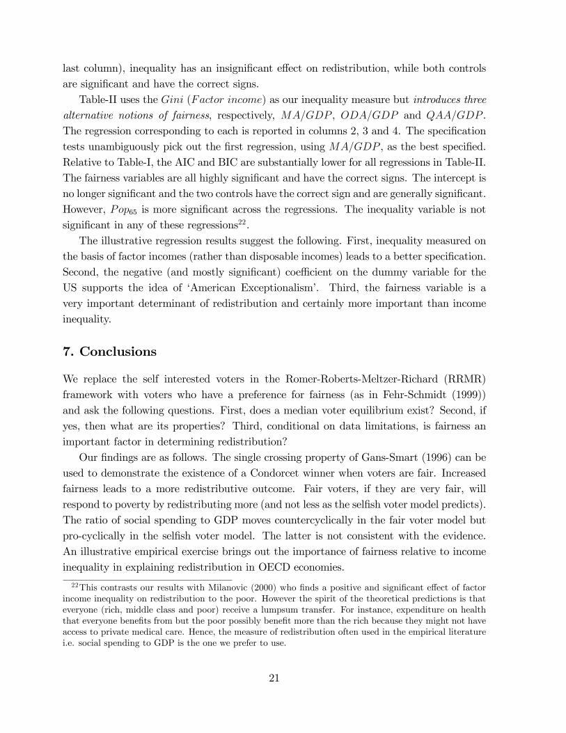
last column), inequality has an insigni�cant e¤ect on redistribution, while both controlsare signi�cant and have the correct signs.Table-II uses the Gini (Factor income) as our inequality measure but introduces three
alternative notions of fairness, respectively, MA=GDP , ODA=GDP and QAA=GDP .The regression corresponding to each is reported in columns 2, 3 and 4. The speci�cationtests unambiguously pick out the �rst regression, using MA=GDP , as the best speci�ed.Relative to Table-I, the AIC and BIC are substantially lower for all regressions in Table-II.The fairness variables are all highly signi�cant and have the correct signs. The intercept isno longer signi�cant and the two controls have the correct sign and are generally signi�cant.However, Pop65 is more signi�cant across the regressions. The inequality variable is notsigni�cant in any of these regressions22.The illustrative regression results suggest the following. First, inequality measured on
the basis of factor incomes (rather than disposable incomes) leads to a better speci�cation.Second, the negative (and mostly signi�cant) coe¢ cient on the dummy variable for theUS supports the idea of �American Exceptionalism�. Third, the fairness variable is avery important determinant of redistribution and certainly more important than incomeinequality.
7. Conclusions
We replace the self interested voters in the Romer-Roberts-Meltzer-Richard (RRMR)framework with voters who have a preference for fairness (as in Fehr-Schmidt (1999))and ask the following questions. First, does a median voter equilibrium exist? Second, ifyes, then what are its properties? Third, conditional on data limitations, is fairness animportant factor in determining redistribution?Our �ndings are as follows. The single crossing property of Gans-Smart (1996) can be
used to demonstrate the existence of a Condorcet winner when voters are fair. Increasedfairness leads to a more redistributive outcome. Fair voters, if they are very fair, willrespond to poverty by redistributing more (and not less as the sel�sh voter model predicts).The ratio of social spending to GDP moves countercyclically in the fair voter model butpro-cyclically in the sel�sh voter model. The latter is not consistent with the evidence.An illustrative empirical exercise brings out the importance of fairness relative to incomeinequality in explaining redistribution in OECD economies.
22This contrasts our results with Milanovic (2000) who �nds a positive and signi�cant e¤ect of factorincome inequality on redistribution to the poor. However the spirit of the theoretical predictions is thateveryone (rich, middle class and poor) receive a lumpsum transfer. For instance, expenditure on healththat everyone bene�ts from but the poor possibly bene�t more than the rich because they might not haveaccess to private medical care. Hence, the measure of redistribution often used in the empirical literaturei.e. social spending to GDP is the one we prefer to use.
21

8. Appendix 1: Fairness, Inequality and Redistribution
Table-I: Inequality and Redistribution1 2 3
Constant35:96���
2:8724:791:29
13:220:74
Gini (LIS)�110:21����4:43 - -
Gini (World Bank) -�0:63��1:80 -
Gini (Factor Income) - -�0:34�1:13
DUS3:031:28
�0:14�0:06
�5:47����3:87
Pop651:23��
2:371:19�
1:961:91���
3:78R2 0:72 0:48 0:59F 95:33 31:85 37:32AIC 110:19 122:39 92:76BIC 113:18 125:37 95:08n 20 20 16
Note: t�values in parentheses. Superscript �, ��, � � � denotes signi�cance at the 10%,5% and 1% level respectively.
Table-II: Fairness, Inequality and Redistribution1 (MA/GDP) 2 (ODA/GDP) 3 (QAA/GDP)
Constant7:540:40
4:700:21
6:000:30
Fairness37:58���
3:349:4�
2:1020:59���
2:85
Gini (Factor Income)�0:15�0:42
�0:18�0:45
�0:19�0:51
DUS�2:90�1:75
�3:61���2:73
�3:85����3:33
Pop651:23���
4:821:63���
5:791:58���
6:03R2 0:80 0:72 0:71F 92:41 65:20 0:55AIC 85:20 88:93 89:10BIC 89:06 92:01 92:19n 16 16 16
Note: t�values in parentheses. Superscript �, ��, � � � denotes signi�cance at the 10%,5% and 1% level respectively.
22

9. Appendix 2: Proofs
9.1. Proof of Lemma 1
From (2.14) we see that, given t; b and si, U (li; t; b; si) is a continuous function of li on thenon-empty compact set [0; 1]. Hence, a maximum exists. Since u is thrice di¤erentiable,so is U and, from (2.14), we get
@U
@li(li; t; b; si) = (1� t) si � l
1�i , (9.1)
@U
@li(0; t; b; si) = (1� t) si, (9.2)
@U
@li(1; t; b; si) = (1� t) si � 1, (9.3)
@2U
@l2i(li; t; b; si) = �1
�l1���
i . (9.4)
First, consider the case t = 1. From (2.14), or (9.1), we see that U (li; 1; b; si) is a strictlydecreasing function of li for li > 0. Hence, the optimum must be
li = 0 at t = 1: (9.5)
Now, suppose t 2 [0; 1). From (2.1), (2.2), (2.6), (9.2) and (9.3) we get that @U@li(0; t; b; si) >
0 and @U@li(1; t; b; si) < 0. Hence an optimal value for li must lie in (0; 1) and, hence, must
satisfy @U@li(li; t; b; si) = 0. From (9.1) we then get
li = (1� t)� s�i , (9.6)
which, therefore, must be the unique optimal labour supply (this also follows from (9.4)).For t = 1, (9.6) is consistent with (9.5). Hence, for each consumer, i, (9.6) gives theoptimal labour supply for each t 2 [0; 1]. �
9.2. Proof of Lemma 2
The proof follows from (2.18) by direct calculation. �
9.3. Proof of Lemma 3
(Existence of a maximum): From (2.19), we see that wi (t; s) is a continuous function oft 2 [0; 1], for i = 1; 2; :::; n. Hence, from (2.26), (2.27) or (2.28), we see that Wj (t; �; �; s)
is also a continuous function of t 2 [0; 1]. Hence, Wj (t; �; �; s) attains a maximum atsome tj 2 [0; 1]. �
23

9.4. Proof of Proposition 1
From (2.24) and Lemma 2(c) it follows for j = 1; ::; n� 1;
@Vj+1@t
� @Vj@t
= � (1� t)��1� j�
n� 1 +(n� j)�n� 1
��s1+�j+1 � s1+�j
�, (9.7)
From (2.1), (2.21), (2.22) and (9.7), it follows that
@Vj+1@t
� @Vj@t
< 0, t 2 [0; 1), j = 1; 2; :::; n� 1. (9.8)
From (2.23)
@Vj@b
=@v (t; b; sj)
@b� �
n� 1Pk>j
�@v (t; b; sk)
@b� @v (t; b; sj)
@b
�� �
n� 1Pi<j
�@v (t; b; sj)
@b� @v (t; b; si)
@b
�(9.9)
From Lemma 2(a) and (9.9)@Vj@b
= 1. (9.10)
From (9.8) and (9.10) we get
�@Vj@t=@Vj@b
is strictly increasing in j: (9.11)
From Lemmas 4 and (9.11) we get that �single-crossing�holds. Hence, from 5, we get thatthe median-voter is decisive, i.e., a majority chooses the tax rate that is optimal for themedian-voter. �
9.5. Proof of Lemma 6
From (2.1), (2.6), (2.19), (2.21), (2.22), (2.26) and (2.12), we get:
@wj@t
= � (1� t)� s1+�j +(1� t)�
n�ni=1s
1+�i � �t (1� t)
��1
n�ni=1s
1+�i , for t < 1, (9.12)
@wm@t
= � (1� t)� s1+�m +(1� t)�
n�ni=1s
1+�i � �t (1� t)
��1
n�ni=1s
1+�i , for t < 1, (9.13)
@wm@t
� @wi@t
= � (1� t)��s1+�m � s1+�i
�, for t < 1, (9.14)
@wk@t
� @wm@t
= � (1� t)��s1+�k � s1+�m
�, for t < 1, (9.15)
24

@2wj@t2
= � (1� t)��1 s1+�j � � (1� t)��1
n�ni=1s
1+�i � � (1� t)
��1
n�ni=1s
1+�i
�� (1� �) t (1� t)��2
n�ni=1s
1+�i , for t < 1, (9.16)
@2wm@t2
= � (1� t)��1 s1+�m � � (1� t)��1
n�ni=1s
1+�i � � (1� t)
��1
n�ni=1s
1+�i
�� (1� �) t (1� t)��2
n�ni=1s
1+�i , for t < 1, (9.17)
@2wm@t2
= �� (1� t)��1�1
n�ni=1s
1+�i � s1+�m
�� � (1� t)
��1
n�ni=1s
1+�i
�� (1� �) t (1� t)��2
n�ni=1s
1+�i < 0, for t < 1, (9.18)
@2wm@t2
� @2wi@t2
= � (1� t)��1�s1+�m � s1+�i
�> 0, for i < m, for t < 1, (9.19)
@2wk@t2
� @2wm@t2
= � (1� t)��1�s1+�k � s1+�m
�> 0, for k > m, for t < 1, (9.20)
Wm = t (1� t)�1
n�ni=1s
1+�i + (1� t)1+�
�s1+�m � �
1 + �s1+�m
�� (1� t)1+�
�
n� 11
1 + �
Pk>m
�s1+�k � s1+�m
�+
�
n� 11
1 + �
Pj<m
�s1+�m � s1+�j
�!. (9.21)
@Wm
@t= (1� t)�
�1
n�ni=1s
1+�i � s1+�m � t�
1� t1
n�ni=1s
1+�i
�+
(1� t)���
n� 1Pk>m
�s1+�k � s1+�m
�+
�
n� 1Pi<m
�s1+�m � s1+�i
��, for t < 1, (9.22)
@2Wm
@t2=@2wm (t; s)
@t2� �
n� 1Pk>j
�@2wk@t2
� @2wm@t2
�� �
n� 1Pi<j
�@2wm@t2
� @2wi@t2
�< 0, for t < 1. (9.23)
Set @Wm
@t= 0 in (9.22) and solve to get
tm =
1n�ni=1s
1+�i � s1+�m + �
n�1Pk>m
�s1+�k � s1+�m
�+ �
n�1Pi<m
�s1+�m � s1+�i
�1+�n�ni=1s
1+�i � s1+�m + �
n�1Pk>m
�s1+�k � s1+�m
�+ �
n�1Pi<m
�s1+�m � s1+�i
� . (9.24)
25

Hence, clearly,0 < tm < 1. (9.25)
In the light of (9.23), Wm (t; �; �; s) attains a unique global maximum on (0; 1) at t = tm.We shall show that this is also the unique global maximum on [0; 1]. From (2.1), (2.12),(2.16), (2.21), (2.22) and (9.22) we get�@Wm
@t
�t=0
=1
n�ni=1s
1+�i � s1+�m +
�
n� 1Pk>m
�s1+�k � s1+�m
�+
�
n� 1Pi<m
�s1+�m � s1+�i
�> 0
(9.26)Hence, t = tm is the unique global maximum of Wm (t; �; �; s) on [0; 1). Next, from (9.21),we get
Wm (1; �; �; s) = 0, (9.27)
and, from (2.1), (2.12), (2.16), (2.21), (2.22), (9.21) and (9.24),
Wm (tm; �; �; s) =
1
1 + �
"1
�
�1
n�ni=1s
1+�i � s1+�m
�+
�
n� 1Pk>m
�s1+�k � s1+�m
�+
�
n� 1Pj<m
�s1+�m � s1+�j
�#
�
264 �n�ni=1s
1+�i
�n�ni=1s
1+�i + 1
n�ni=1s
1+�i � s1+�m + �
n�1Pk>m
�s1+�k � s1+�m
�+ �
n�1Pi<m
�s1+�m � s1+�i
�3751+�
> 0.
(9.28)
From (9.27) and (9.28), we see that t = tm is the unique global maximum ofWm (t; �; �; s)
on [0; 1]. �
9.6. Proof of Proposition 2
Let
x =1
n�ni=1s
1+�i � s1+�m +
�
n� 1Pk>m
�s1+�k � s1+�m
�+
�
n� 1Pi<m
�s1+�m � s1+�i
�: (9.29)
From Lemma 6 and (9.29), we get
tm =1
1 + �nx�ni=1s
1+�i
, where x > 0 and�
n�ni=1s
1+�i > 0. (9.30)
It follows that an increase in x will increase tm. In particular, an increase in � or anincrease in � (or both) will increase tm. This establishes part (a). It also follows that afair median voter (� > 0; � > 0) will vote for a higher tax rate than a sel�sh median voter
26

(� = � = 0). This establishes part (b).
For j > m,@tm@sj
=
� (1 + �) s�j
��1 + �
n�1 +���2
�s1+�m + �+�
n�1Pi<m
s1+�i
�n
�1+�n�ni=1s
1+�i � s1+�m + �
n�1Pk>m
�s1+�k � s1+�m
�+ �
n�1Pi<m
�s1+�m � s1+�i
��2 > 0. (9.31)
Hence, an increase in the skill of voter-workers above the median will increase the tax rate,whether the median voter is sel�sh or fair. This establishes part (c).
@tm@sm
= (9.32)
�� (1 + �) s�m
�s1+�m +
�1 + ���
2
��ni=1s
1+�i + �
n�1Pk>m
�s1+�k � s1+�m
�+ �
n�1Pi<m
�s1+�m � s1+�i
��n
�1+�n�ni=1s
1+�i � s1+�m + �
n�1Pk>m
�s1+�k � s1+�m
�+ �
n�1Pi<m
�s1+�m � s1+�i
��2 < 0,
Hence, for sel�sh and fair voters alike, a reduction of the skill of the median voter withincrease the tax rate. Conversely, an increase in the skill of the median voter will reducethe tax rate. This establishes part (d).
For j < m,@tm@tj
=
� (1 + �) s�j
�s1+�m � �
n�1Pk>m
�s1+�k � s1+�m
�� �
n�1
��ni=1s
1+�i +
Pi<m
�s1+�m � s1+�i
���n
�1+�n�ni=1s
1+�i � s1+�m + �
n�1Pk>m
�s1+�k � s1+�m
�+ �
n�1Pi<m
�s1+�m � s1+�i
��2 , (9.33)
Part (f) follows from (9.33) since the coe¢ cients of � and � in the numerator are positive.Set � = � = 0 in (9.33) to get, for a sel�sh median voter,
� = � = 0) for j < m,@tm@tj
=� (1 + �) s�js
1+�m
n�1+�n�ni=1s
1+�i � s1+�m
�2 > 0, (9.34)
Thus, a sel�sh median voter responds to a reduction in the skill of consumers below themedian by reducing the tax rate. This establishes part (e). Recall, from Remark 1, thatthe tax rate in our model equals the ratio of social spending to aggregate income. Hence, tothe extent that low skill workers are more adversely a¤ected in a recession, the sel�sh votermodel predicts pro-cyclic movement of the ratio of social spending to aggregate income.Also, from (9.33), it follows that
for j < m,@tm@tj
< 0, if � or � is su¢ ciently large. (9.35)
27
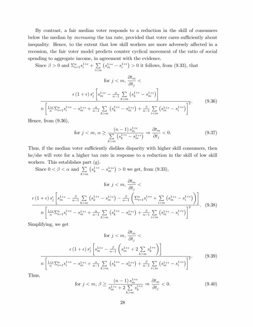
By contrast, a fair median voter responds to a reduction in the skill of consumersbelow the median by increasing the tax rate, provided that voter cares su¢ ciently aboutinequality. Hence, to the extent that low skill workers are more adversely a¤ected in arecession, the fair voter model predicts counter cyclical movement of the ratio of socialspending to aggregate income, in agreement with the evidence.Since � > 0 and �ni=1s
1+�i +
Pi<m
�s1+�m � s1+�i
�> 0 it follows, from (9.33), that
for j < m,@tm@tj
<
� (1 + �) s�j
�s1+�m � �
n�1Pk>m
�s1+�k � s1+�m
��n
�1+�n�ni=1s
1+�i � s1+�m + �
n�1Pk>m
�s1+�k � s1+�m
�+ �
n�1Pi<m
�s1+�m � s1+�i
��2 . (9.36)
Hence, from (9.36),
for j < m, � � (n� 1) s1+�mPk>m
�s1+�k � s1+�m
� ) @tm@tj
< 0. (9.37)
Thus, if the median voter su¢ ciently dislikes disparity with higher skill consumers, thenhe/she will vote for a higher tax rate in response to a reduction in the skill of low skillworkers. This establishes part (g).Since 0 < � < � and
Pk>m
�s1+�k � s1+�m
�> 0 we get, from (9.33),
for j < m,@tm@tj
<
� (1 + �) s�j
�s1+�m � �
n�1Pk>m
�s1+�k � s1+�m
�� �
n�1
��ni=1s
1+�i +
Pi<m
�s1+�m � s1+�i
���n
�1+�n�ni=1s
1+�i � s1+�m + �
n�1Pk>m
�s1+�k � s1+�m
�+ �
n�1Pi<m
�s1+�m � s1+�i
��2 . (9.38)
Simplifying, we get
for j < m,@tm@tj
<
� (1 + �) s�j
�s1+�m � �
n�1
�s1+�m + 2
Pk>m
s1+�k
��n
�1+�n�ni=1s
1+�i � s1+�m + �
n�1Pk>m
�s1+�k � s1+�m
�+ �
n�1Pi<m
�s1+�m � s1+�i
��2 . (9.39)
Thus,
for j < m, � � (n� 1) s1+�m
s1+�m + 2Pk>m
s1+�k
) @tm@tj
< 0. (9.40)
28

Hence, provided the median voter cares su¢ ciently about consumers with lower skill,he/she will vote for a higher tax rate in response to a reduction in the skill of low skillworkers. However, we need to check that the lower bound on � in (9.40) is feasible, i.e.,is consistent with � < 1. That this is the case, is established by (9.41), below, using (2.1)and the fact that n = 2m� 1.
(n� 1) s1+�m
s1+�m + 2Pk>m
s1+�k
<2 (m� 1)
1 + 2 (m� 1) < 1 (9.41)
This completes the proof of part (h). �
9.7. Proof of Lemma 7
From (2.15) and (2.18), the indirect utility corresponding to pretax income can be writtenas 1�t
1+�yi + b. Hence, for our model, the two inequality measures, di¤erence-dominance
(Marshall and Olkin, 1979) and utility-gap dominance (Zheng, 2007), coincide. �
9.8. Proof of Proposition 3
Proof : Let tm and Tm be the tax rates corresponding to pretax income vectors x 2 I andy 2 I, respectively. Then, from (2.15) and Lemma 6
tm =
1n�ni=1xi � xm + �
n�1Pk>m
(xk � xm) + �n�1
Pi<m
(xm � xi)
1+�n�ni=1xi � xm + �
n�1Pk>m
(xk � xm) + �n�1
Pi<m
(xm � xi), (9.42)
Tm =
1n�ni=1yi � ym + �
n�1Pk>m
(yk � ym) + �n�1
Pi<m
(ym � yi)
1+�n�ni=1yi � ym + �
n�1Pk>m
(yk � ym) + �n�1
Pi<m
(ym � yi). (9.43)
Let x and y be de�ned by:
x =1
n�ni=1xi � xm +
�
n� 1Pk>m
(xk � xm) +�
n� 1Pi<m
(xm � xi) , (9.44)
y =1
n�ni=1yi � ym +
�
n� 1Pk>m
(yk � ym) +�
n� 1Pi<m
(ym � yi) , (9.45)
thentm =
x
x+ �n�ni=1xi
=1
1 + �nx�ni=1xi
, (9.46)
Tm =y
y + �n�ni=1yi
=1
1 + �ny�ni=1yi
. (9.47)
If x di¤erence dominates y (De�nition 2), then 0 < x � y. Hence, tm � Tm. If x strictlydi¤erence dominates y, then 0 < x < y. Hence, tm < Tm. �
29

References
[1] Ackert, L. F., J. Martinez-Vazquez, M. Rider (2004). Tax policy design in the presenceof social preferences: Some experimental evidence. Georgia State University Interna-tional Studies Program. Working Paper No. 04-25.
[2] Alesina, A. and G-M. Angeletos (2003). Fairness and Redistribution, mimeo. HarvardUniversity.
[3] Alesina, A. and D. Rodrik (1994). Distributive politics and economic growth. Quar-terly Journal of Economics, 109, 465-490.
[4] Atkinson A (1970) On the measurement of inequality. Journal of Economic Theory2:244-263.
[5] Auerbach, A. (2003). Is there a role for discretionary �scal policy? University ofMichigan Law School, mimeo.
[6] Benabou R. (2000) Unequal societies: Income distribution and the social contract.The American Economic Review, vol.90, no.1, 96-129.
[7] Benabou R. and E A Ok (2001) Social mobility and the demand for redistribution:The POUM hypothesis. The Quarterly Journal of Economics, May, 447-487.
[8] Black, D. (1948). On the rationale of group decision making. Journal of PoliticalEconomy 56: 23-34.
[9] Bolton, E. B. and A. Ockenfels (2000). ERC: A theory of equity, reciprocity, andcompetition. American Economic Review, 90, 166-193.
[10] Camerer, C. (2003). Behavioral Game Theory. Russell Sage Foundation.
[11] Dhami, S. and al-Nowaihi (2007). Fairness and direct democracy. University of Leices-ter Discussion Paper in Economics 06/11.
[12] Easterly, W. and S. Rebelo (1993). Fiscal policy and economic growth: An empiricalinvestigation. Journal of Monetary Economics, 32: 417-58.
[13] Fehr, E. and K. M. Schmidt (1999). A theory of fairness, competition and cooperation.Quarterly Journal of Economics, 114, 817-868.
[14] Galasso, V. (2003). Redistribution and fairness: a note. European Journal of PoliticalEconomy, 19 (4), 885-892.
30

[15] Galasso, V. and J. I. Conde Ruiz (2005). Positive Arithmetic of the Welfare State.Journal of Public Economics 89: 933-955.
[16] Gans, J. S. and M. Smart (1996). Majority voting with single-crossing preferences.Journal of Public Economics, 59, 219-237.
[17] Glaeser, E. L. (2005). Inequality. NBER working paper no. 11511.
[18] Lindert, P. H. (2003). Whence the welfare state. Paper presented at the December2003 conference on political institutions and economic policy, Harvard University.
[19] Lindert, P. H. (1996). What limits social spending? Explorations in Economic History,33, 1-34.
[20] Marshall A, Olkin I (1979) Inequalities: theory of majorization and its applications.Academic, New York.
[21] Matsusaka, J. G. (2005a). Direct democracy works. Journal of Economic Perspectives.19, 185-206.
[22] Matsusaka, J. G. (2005b). The eclipse of legislatures: Direct democracy in the 21stcentury. Public Choice, 124, 157-178.
[23] Meltzer, A. H. and S. F. Richard (1981). A rational theory of the size of government.Journal of Political Economy, 89, 914-927.
[24] Milanovic, B. (2000). The median voter hypothesis, income inequality, and incomeredistribution: an empirical test with the required data. European Journal of PoliticalEconomy, 16, 367-410.
[25] OECD Social expenditure database 1980-1996.
[26] OECD in �gures: statistics on the member countries, 2004 edition.
[27] Perotti, E. C. (1996). Growth, income distribution and democracy: What the datasay. Journal of Economic Growth, 1, 149-188.
[28] Persson, T. and G. Tabellini (1994). Is inequality harmful for growth? AmericanEconomic Review, 84, 600-621.
[29] Persson, T. and G. Tabellini (2000). Political Economics. Cambridge, MA: MIT Press.
[30] Piketty, T. (1995). Social mobility and redistributive politics. Quarterly Journal ofEconomics, 110, 551-584.
31
[31] Preston, I. (1990) Ratios, di¤erences and inequality indices. Mimeo., Nu¢ eld College,Oxford.
[32] Preston, I. (2006) Inequality and Income gaps. Institute of Fiscal Studies WorkingPaper No. 06/25.
[33] Rabin, M. (1993). Incorporating fairness into game theory and economics. AmericanEconomic Review, 83, 1281-1302.
[34] Roberts, K. W. (1977). Voting over income tax schedules. Journal of Public Eco-nomics, 8, 329-340.
[35] Romer, T. (1975). Individual welfare, majority voting, and the properties of a linearincome tax. Journal of Public Economics, 4, 163-185.
[36] Roodman, D. (2005). An index of donor performance. Centre for Global DevelopmentWorking paper No. 67.
[37] Smeeding, T. (2002). Globalization, inequality and the rich countries of the G-20: Evi-dence from the Luxembourg income study (LIS). Luxembourg Income Study WorkingPaper No. 320.
[38] Tabellini, G. (1991). The politics of intergradational redistribution. Journal of Polit-ical Economy 99: 335-57.
[39] Tyran, J-R. and R. Sausgruber (2006). A little fairness may induce a lot of redistrib-ution in a democracy. European Economic Review, 50, 469-85.
[40] Zheng, B. (2007) Utility-gap dominances and inequality orderings. Social Choice andWelfare, 28, 255-280.
32