Facies Modeling Accounting for the Precision and Scale ofSeismic Data: Application to Albacora Field

G. Schwedersky-Neto, Marcella Maria de Melo Cortez, and Marcos Fetter LopesPetrobras CENPES Research Center

C. V. Deutsch,Department of Civil & Environmental Engineering, University of Alberta

Abstract

Seismic impedance provides information on the relative proportion of different facies types.It is important to integrate such seismic data in the construction of detailed 3-D faciesmodels, which are used for reservoir management. Two critical challenges faced in theintegration of seismic impedance data: (1) the seismic data is at a larger scale than thewell data / geological modeling cells, and (2) the seismic data provides soft (imprecise)information on the facies proportions within that large volume.

A novel block cokriging approach was developed and implemented. This method wasadapted for use in sequential indicator simulation to explicitly account for the large scalesoft seismic data. Conventional sequential indicator simulation and a popular alternative,SIS with Bayesian updating, were considered for comparison purposes.

The key challenge in applying stochastic simulation with block cokriging is the construc-tion of a licit model of coregionalization between the “hard” well data and the “soft” seismicdata. A hybrid procedure is presented that can be applied in the common case of limited welldata.

The Albacora field offshore Brazil consists of deep water turbidite sands, shales, andcemented sands. Good quality seismic data and significant variations in facies proportionsmake this an excellent example to illustrate the benefit of integrating seismic data in highresolution 3-D facies modeling.

KEYWORDS: geostatistical simulation, stochastic modeling, reservoir characterization,Bayesian updating, block cokriging

Introduction

One goal of reservoir modeling teams is to build high resolution predictive reservoir modelsof facies, porosity, and permeability that, by construction, honor all available reservoir data.These numerical models provide reliable predictions of future reservoir performance at allstages of the reservoir life cycle. The unavoidable uncertainty in reservoir performanceforecasting will be measured and minimized by such reliable numerical reservoir models.

1

The available data includes, but is not limited to, conceptual geological models, seismicdata, core data, well log data, DST/RFT data, well test data, and historical productiondata. Each source of data carries information, at different scales and with varying levelsof precision, related to the true distribution of petrophysical and fluid properties in thereservoir. Integrating all available data by construction in numerical geological models willmake it possible for reservoir management teams to quickly consider numerous scenarios tooptimize each reservoir management plan.

Observations and interpretations related to seismic data are particularly difficult tobuild into predictive reservoir models. This paper addresses this challenging aspect ofdata integration. Seismic data is important because it provides information in the vastinterwell region; most other data provides information only within small localized volumes.The challenge is to build high resolution models that account for the large scale impreciseseismic data [3, 6, 8, 10].

Seismic-derived acoustic impedance data provides information on facies types and poros-ity. The emphasis of this paper is modeling facies types; the facies types are, in general,more important since they constrain the allowable range of porosity, permeability, and rel-ative permeability. There are two different approaches to facies modeling (1) cell-basedfacies modeling where the spatial distribution of the facies types is statistically constrainedwith n-point statistics such as variograms and transition probabilities, and (2) object-basedfacies modeling where the spatial distribution of facies types is created with geologicallyrealistic objects embedded within a matrix facies type. The choice of the most appropriatemethod depends on the depositional environment, the relative proportions of the differentfacies types, and the presence of diagenetic overprint.

Both approaches have their place; however, a cell-based approach is considered mostappropriate for the Albacora reservoir, which was the focus of the case study. The mainreason for this choice is the diagenetic cements, which defy simple object parameterization.

There are a number of different cell-based facies modeling techniques. Indicator sim-ulation provides great flexibility, particularly for the integration of seismic data, and wasused in this study. A common alternative cell-based approach is based on truncating con-tinuous Gaussian fields [14]. This approach was not used because of the implicit nesting ofthe variables and the inflexibility or only one varigoram. It is worth noting, however, thatthe “variogram downscaling” procedures developed below could be applied for truncatedGaussian simulation.

At the heart of indicator simulation is the use of kriging (spatial regression) to determinethe conditional probability of each facies type. In presence of seismic data the krigingequations must be modified to weight the seismic data, a procedure called cokriging. Suchcokriging requires a model for the spatial correlation of the facies types, the seismic data,and the cross correlation between facies types and seismic data. Inference of these modelsof spatial correlation is the critical problem. In addition to the mathematical constraintson such “models of coregionalization,” a confounding factor is that the seismic data is at asignificantly larger scale that the well-derived indicator data. The requirement is a smallscale model of coregionalization; otherwise, the cross correlation depends not only on thedistance h between the seismic and well data but on the relative position of the well datawithin the larger seismic data volume. One procedure for inference of the required modelof coregionalization will be developed below [5].

2

The conventional sequential indicator simulation (SIS) procedure is modified to performcokriging with large scale seismic data and small scale well data. This modified procedureexplicitly accounts for the scale and precision of the seismic data. An alternative to thissomewhat complex procedure is the “Bayesian updating” approach [8], which requires onlythe correlation (variogram) of the well data. This simpler procedure will also be consideredin the case study.

The Albacora reservoir is an offshore Brazilian reservoir consisting of deepwater tur-bidite sands and shale. The four facies of interest are (1) clean turbidite sandstone witha minor fraction of concretions, (2) sandstone with a significant proportion of concretions,(3) sandstone with significant concretions mixed with shale, and (4) clearly non-reservoirfacies consisting of shale and entirely cemented sandstone. The spatial distribution of thesefacies types has an overwhelming effect on fluid flow. A reservoir characterization study wasundertaken to model the facies distribution. Good quality 3-D seismic data are availableover the study area; the inverted impedance values are sensitive to the amount of reservoir/ non-reservoir, thus is importance to include in the reservoir characterization study. Thefinal facies models will be used for reservoir management decision making. The focus of thispaper is on methods to construct facies models consistent with the well and seismic data.

Methodology

There are k = 1, . . . ,K facies types with overall average proportions of pk, k = 1, . . . ,Kwhere

∑Kk=1 pk = 1. Local well data at location u are represented as a series of K indicator

data defined as:

i(u; k) =

{

1, if facies k prevails at location u

0, otherwisek = 1, . . . ,K (1)

The expected values (averages) of the indicator data correspond to the global proportionspk, k = 1, . . . ,K.

The notation p(uβ ; k), k = 1, . . . ,K will be used for the seismic-derived probability offacies k at block location uβ. The modeling scale (associated to the hard well data scale)will be denoted with a v and the seismic scale will be denoted with a V . The notation |v|or |V | refers to the measure or dimension of the well and seismic data, respectively. Thismeasure depends on direction. For example, the seismic data V is larger than the well datav in the vertical direction whereas it may coincide, or even be smaller than, the modelingcell size v in the horizontal direction.

Sequential Indicator Simulation

The sequential indicator simulation (SIS) approach provides flexibility to integrate soft dataand unique patterns of spatial correlation. An object-based approach would be difficult toapply given the lack of clear object geometries; the shales and diagenetic cements do notfollow any obvious object parameterization. The SIS methodology:

1. Loop over all cells in the 3-D model in random order.

2. At each cell location:

3

(a) Find nearby data: (1) well data, (2) cells that have already been informed earlierin the path, and (3) seismic data

(b) Estimate the probability of each facies, k = 1, . . . ,K (where K=4 in our case)by kriging:

i∗(u; k) =nw∑

α=1

λα · i(uα; k) +ns∑

β=1

λ′

β · p(uβ ; k) (2)

where i∗(u; k), k = 1, . . . ,K are the probabilities of facies k = 1, . . . ,K to bepresent at location u, nw is the number of nearby well data and previouslyinformed cells, λα, α = 1, . . . , nw are the weights they receive, i(uα; k) is theprobability that location uα is in facies k (0 or 1 for these hard data), ns is thenumber of nearby seismic data, λ′

β, β = 1, . . . , ns are the weights they receive,and p(uβ; k) is the probability that location uβ is in facies k (between 0 to 1depending on the acoustic impedance and the calibration with well data).

A common assumption is to take the single collocated seismic value and builda model of coregionalization that depends solely on the collocated correlationcoefficient [2, 3, 15]. A number of studies have considered the impact ot thisassumption [6].

(c) Assemble the estimated probabilities into a cumulative distribution. The order-ing does not matter as long as the random number (next step) is not correlatedwith the ordering.

(d) Draw a random number between 0 and 1 and read the corresponding facies codek′ from cumulative distribution.

(e) Assign the facies code k′ to the location u.

3. Return to 2 until every cell in the model has been assigned a facies code

4. Repeat with different random number seeds for multiple equally probably realizations.

This procedure is classical [1]. The key step for our purposes is how to establish the “correct”weights to give to the well data and the seismic data. There are three variants of SIS that wewill consider (1) well data alone, (2) the Bayesian updating approach for simply integratingseismic data, and (3) a block cokriging approach for rigorous integration. The followingsteps are required to implement SIS.

Seismic-Derived Probabilities

The seismic attribute(s) or acoustic impedance (AI) must be calibrated with the faciesproportions. We should note that cokriging does not require this calibration; the originalAI units could be retained and the calibration could enter through the cross variogrambetween the hard “i” data and soft “AI” data. Notwithstanding the flexibility of cokrigingto handle untransformed AI units, we prefer the calibrated p(u;k) values for a number ofreasons (1) the cross variogram may be poorly informed with limited well data, and (2)the proportion / probability data are easier to interpret; they are in units we understand.There are alternative approaches to seismic calibration including [11].

4

ai-class p(uβ; k = 1, ai) p(uβ; k = 2, ai) p(uβ ; k = 3, ai) p(uβ; k = 4, ai)

−∞ - ai1ai1 - ai2ai2 - ai3

. . .ai9 - ∞

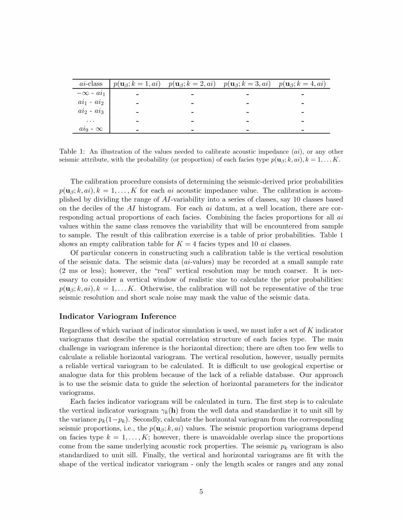
Table 1: An illustration of the values needed to calibrate acoustic impedance (ai), or any otherseismic attribute, with the probability (or proportion) of each facies type p(uβ; k, ai), k = 1, . . .K.

The calibration procedure consists of determining the seismic-derived prior probabilitiesp(uβ; k, ai), k = 1, . . . ,K for each ai acoustic impedance value. The calibration is accom-plished by dividing the range of AI-variability into a series of classes, say 10 classes basedon the deciles of the AI histogram. For each ai datum, at a well location, there are cor-responding actual proportions of each facies. Combining the facies proportions for all aivalues within the same class removes the variability that will be encountered from sampleto sample. The result of this calibration exercise is a table of prior probabilities. Table 1shows an empty calibration table for K = 4 facies types and 10 ai classes.

Of particular concern in constructing such a calibration table is the vertical resolutionof the seismic data. The seismic data (ai-values) may be recorded at a small sample rate(2 ms or less); however, the “real” vertical resolution may be much coarser. It is nec-essary to consider a vertical window of realistic size to calculate the prior probabilities:p(uβ; k, ai), k = 1, . . . K. Otherwise, the calibration will not be representative of the trueseismic resolution and short scale noise may mask the value of the seismic data.

Indicator Variogram Inference

Regardless of which variant of indicator simulation is used, we must infer a set of K indicatorvariograms that descibe the spatial correlation structure of each facies type. The mainchallenge in variogram inference is the horizontal direction; there are often too few wells tocalculate a reliable horizontal variogram. The vertical resolution, however, usually permitsa reliable vertical variogram to be calculated. It is difficult to use geological expertise oranalogue data for this problem because of the lack of a reliable database. Our approachis to use the seismic data to guide the selection of horizontal parameters for the indicatorvariograms.

Each facies indicator variogram will be calculated in turn. The first step is to calculatethe vertical indicator variogram γk(h) from the well data and standardize it to unit sill bythe variance pk(1−pk). Secondly, calculate the horizontal variogram from the correspondingseismic proportions, i.e., the p(uβ ; k, ai) values. The seismic proportion variograms dependon facies type k = 1, . . . ,K; however, there is unavoidable overlap since the proportionscome from the same underlying acoustic rock properties. The seismic pk variogram is alsostandardized to unit sill. Finally, the vertical and horizontal variograms are fit with theshape of the vertical indicator variogram - only the length scales or ranges and any zonal

5

anisotropy is taken from the seismic proportion variogram.There are a number of assumptions in this hybrid approach to determine indicator

variograms. The most important assumption is that the pk variogram provides a reasonableapproximation to the horizontal indicator i range. This is reasonable if the seismic iswell correlated to the facies proportions and if the vertical averaging of the seismic is nottoo pronounced. A second constraint is that we cannot identify zonal anisotropy becausewe have no consistent 3-D dataset for variogram calculation. This is probably incorrect;however, no other data is available to assist us with inference. Notwithstanding theselimiting assumptions, there is little alternative in presence of limited “hard” well data. Ofcourse, experience from other better-drilled reservoirs in the same basin could be used.

An example of the steps in this procedure is presented later with the case study.

The Bayesian Updating Approach

No further inference is required to apply the Bayesian Updating Approach to integrate theseismic data in SIS; the indicator variograms and calibration are sufficient. This method isgaining in popularity because of its simplicity and ease with which seismic is accounted for[7, 8, 9].

At each location along the random path (recall procedure described above), indicatorkriging is used to estimate the i∗(u; k), k = 1, . . . ,K values from hard i data alone, thenthe probabilities are modified (updated) as follows:

i∗∗(u; k) = i∗(u; k) ·p(uβ ; k, ai)

pk

· C k = 1, . . . ,K (3)

where i∗∗(u; k) are the updated probabilities for simulation, p(uβ ; k, ai) is the seismic-derived probability of facies k at location u being considered, pk is the overall proportion offacies k, and C is a normalization constant to ensure that the sum of the final probabilitiesis 1.0. The factor p(uβ; k, ai)/pk operates to increase or decrease the probability dependingon the difference of the calibrated facies proportion from the global proportion.

The simplicity and utility of this approach is appealing. There are two implicit assump-tions behind Bayesian updating that may be important (1) the collocated seismic dataperfectly screens nearby seismic data - a Markov type model of coregionalization or crossvariability between seismic and facies indicator, and (2) the scale of the seismic is implicitlyassumed to be the same as the geological cell size. The block cokriging approach is theo-retically more rigorous and can be consdered for comparison purposes. The first step in thecokriging process is to infer a licit model of coregionalization.

Cross/Seismic Variogram Inference

The premise of this paper is that rigorous accounting of the scale and precision of seismicdata leads to better reservoir models. As stated above, this calls for a seismic variogramand a cross well-seismic variogram at a small scale. The inference of such variogram modelsis critical to the proposed method.

Cokriging requires i, i − p, and p variograms at a small scale for all facies types, k =1, . . . ,K. At this point we only have the i variograms that have been defined from both well

6

data and seismic data. Cokriging requires a positive definite model of coregionalization.In particular, the linear model of coregionalization (LMC) is used almost exclusively ingeostatistics [12]. For each facies k = 1, . . . ,K the LMC model would take the form:

γi,i(h) = C1

i,i + C2

i,i · Γ2(h) + C3

i,i · Γ3(h) . . .

γi,p(h) = C1

i,p + C2

i,p · Γ2(h) + C3

i,p · Γ3(h) . . . (4)

γp,p(h) = C1

p,p + C2

p,p · Γ2(h) + C3

p,p · Γ3(h) . . .

where Γj , j = 1, . . . , ns are common variogram models of specified type (spherical, expo-nential, Gaussian, . . . ), range, and anisotropy. Only the sill C parameters are allowed tovary between the three variogram models. Moreover the C values must satisfy the followingconstraints:

Cii,i > 0 ∀ i

Cip,p > 0 ∀ i (5)

Cii,i · C

ip,p > Ci

i,p · Cii,p ∀ i

the underlying hypothesis is that the i and p variables are linear combinations of a commonpool of random variables.

In the present context we have the basic nested structures from our i variogram models.The essential step now is to link the large V scale seismic p, p variogram and the large Vscale cross i, p variogram to small v scale models that can be fit with the linear model ofcoregionalization described above. For illustration, the basic relations to “downscale” a p, pvariogram will be described below, see also [13, 5]. The same procedure may be applied tothe cross variogram.

1. The nugget effect decreases as a variable is averaged to larger scale; the nugget ishigher for small scale data. Since the nugget variance is, by definition, random, thescaling relation is as follows:

[

C0

p

]

v= C0

p ·|V |

|v|(6)

where the v subscript denotes the geological modeling scale, |V | is the size of seismicvolume, and |v| is the size of the geological modeling cells.

2. The ranges of the basic structures are reduced by the size of the averaging volume

av = aV − (|V | − |v|) (7)

where the notation |V | and |v| are used here to denote the dimension of the averagingvolume in different directions. For example, if V and v are the same size in oneparticular direction (say, horizontally) then the range does not change. Of course,the vertical range would almost certainly be different since the V -scale is 10-50 timeslarger than the geological modeling scale.

7

3. The sill of each basic structure is increased for smaller scales. In this case (as comparedto the nugget effect discussed above) we need to account for the specific nature of thevariogram. The scaling relationship:

[

Cjp

]

v= Cj

p ·1 − Γ

j(v, v)

1 − Γj(V, V )

(8)

where the average variogram Γj(v, v) and Γ

j(V, V ) values are the classical “gamma-

bar” values calculated using the point range.

The variance of the small scale p values is the sum of the downscaled C values, that is,[

σ2

p

]

v=

∑

j

[

Cjp

]

v(9)

Where the small scale variance is always greater than the large scale variance; the variancealways decreases when a variable is averaged to a larger scale. Note that we can applythese same relations with the cross variogram. The variance in equation 9 would be a crosscovariance. These relations can be applied directly to “downscale” the sill parameters ofthe seismic pk variograms. The difficulty is inference of the cross i − p variogram, sincethere are too few well data to reliably inform an experimental cross variogram (even in thevertical direction after averaging to the V -scale). We will make two key assumptions toestablish the cross variogram parameters: (1) the sill of the cross variogram is the smallscale cross covariance, and (2) the shape of the cross variogram is the same as the shapeof the direct i, i variogram. These are justifiable since the sill of the cross variogram is thecross covariance unless there is zonal anisotropy and the shape of the direct i, i variogramis certainly related to the cross variogram. Moreover, the LMC requires the same nestedvariogram structures. Therefore, the cross variogram parameters are given by:

Cji,p = Cj

i · [ρi,p]v , j = 0, 1, . . . (10)

where [ρi,p]v is the correlation between the small scale indicator data and seismic data. Acorrelation coefficient has been used rather than a covariance because it is more intuitive tomost people (which makes it easier to check the model parameters before using them). Asa consequence, the sill parameters for the small scale indicator variogram γi,i(h) and thesmall scale seismic variogram γp,p(h) must be normalized to sum to 1.

The small scale correlation coefficient [ρi,p]v can be determined from the large scalecorrelation coefficient [ρi,p]V , which can be calculated from the calibration data. That is,[ρi,p]V is calculated by cross plotting the actual proportion of facies at the well locationsagainst the seismic predictions. The downscaling equations given above are used to calculatethe small scale correlation coefficient. The procedure can be automated and requires nointerpretation, hence it can be left to computer code. The small scale correlation coefficient[ρi,p]v is calculated from the small scale sill / variance values:

[ρi,p]v =

[

σ2

i,p

]

v√

[

σ2

i

]

v

[

σ2p

]

v

(11)

8

where the variance values are given by:

[

σ2

i

]

v=

∑ji

[

Cji

]

v· fj

∑

j

[

Cji

]

v

and[

σ2

p

]

v=

∑jp

[

Cjp

]

v· fj

∑

j

[

Cjp

]

v

(12)

note that the fj values are the scaling factors in downscaling equations 6 and 8.Application of this procedure leads to a complete LMC model of coregionalization that

can be used for block cokriging with the seismic data and well data. Of course, the modelmust be checked to ensure positive definiteness (see 5) and adjusted if necessary.

Block Cokriging

Block cokriging accounts for the scale of the seismic data and the calibration from acousticimpedance to facies proportions. The cokriging formalism is classical; however, most geo-statistical modeling applications consider the different data types to be at the same spatialscale. Once a small scale LMC model of coregionalization has been established, spatialaverages of the variogram (γ or gamma-bar values) are used in the cokriging equations.

Solution of the cokriging system of equations leads to the weights needed by equation(2), that is, the λα and λ′

β weights applied to the hard and soft data. We should commentthat implementation of block cokriging in a conventional SIS program (such as sisim inGSLIB [4]) is straightforward.

Application to Albacora

The offshore Albacora field consists of deep water turbidite sands, shales, and cementedsands. The important upper portion of the reservoir was modeled with seven verticalwells and two horizontal wells. The model was constructed with constant thickness (2.5m) cells conforming to the reservoir top. Based on prior geological work, four facies wereconsidered in the sequential indicator simulation: (1) types 1 & 2.1 (clean sandstone with upto about 15% concretions), (2) type 2.2 (up to 30% concretions), (3) type 3 (about one half acombination of concretions and shale), and (4) types 4 & 5 (non-reservoir). The distinctionbetween facies types 2 and 3 is that 3 has a slightly greater amount of non-reservoir rock andit contains shales that have greater lateral continuity than the concretions. The laterallycontinuous shales of facies type 3 may lead to a reduced vertical permeability.

Figure 1 shows a base map with the seven well locations. A cross section through fourwells showing interpreted geologic correlation is shown on Figure 2. The model describedhere goes from the top of the reservoir to the “B” horizon. The “C” horizon marked on theFigure 2 is largely cemented and is added deterministically after modeling the other faciesstochastically.

Acoustic impedance from the wells and seismic has a strong negative correlation withthe porosity. The porosity distributions within each of the four facies types described aboveare quite different; therefore, it will be possible to use the seismic data to constrain the3-D distribution of facies. The facies were assigned to 2.5 m thick cells. Although thewell log data provide greater resolution, 2.5 m cells are suitable because (1) the originalfacies are defined by observing the concretions, shale, and sand over 1-3 m of core, and

9

(2) the 0.2 m sampling resolution of the well logs is due to the frequent sampling of thetool responses and is not representative of the true volume measured by the well logs. Theacoustic impedance AI is available at an interval of 2 ms. Of course, the resolution is notthat good (2 ms is approximately 4 meters). Each AI datum represents a vertical averageof 4- 8 ms (considered to be about 15 m for this study). This averaging will be consideredin modeling facies through the “block cokriging” approach.

An initial assessment of the value of seismic data is shown on Figure 3, which showsa cross plot of seismic impedance (Y axis) versus the proportion of facies 1 (X axis). Thecorrelation of impedance with the proportions of facies 2, 3, and 4 is not as good (see later).

A horizontal slice through impedance cube is shown on Figure 4. A cross section throughimpedance cube is shown on Figure 5. These slices show significant areal and vertical vari-ations in impedance that, in turn, constrain proportons of facies. Note the low impedanceto the northwest and the high impedance to the south. The vertical variations are quitesmooth.

The seismic impedance was calibrated to facies proportions and four arrays of propor-tions were generated. Figure 6 shows a cross plot of the seismic derived proportion of facies1 (X axis) versus the actual proportion of facies 1 (Y axis). The correlation coefficient hereis 0.61, which is used to establish the linear model of coregionalization described above. Thecorrelation coefficients for the other facies are 0.30, 0.64, and 0.39, respectively for facies 2,3, and 4.

The vertical indicator variogram for facies 1 is shown on Figure 7. Correspondinghorizontal varigorams through cube of seismic derived proportions of facies 1 is shown onFigure 8. A 3-D variogram model can be put together from these 3 directional variograms.A short FORTRAN program was written to take the indicator variograms (the variogramwas different for each of the facies) and perform the downscaling operations presented above.This program also ensures that the result is positive definite.

The indicator variograms could be used directly (before downscaling) to perform se-quential indicator simulation without regard for the seismic data. A horizontal slice andcross section of the sequential indicator simulation model (without using the seismic data)are shown on Figures 9 and reffasimxz. Close examination of the model reveals that thewell data and variograms are honored; of course, the trends revealed in the seismic data arenot honored.

Adding the seismic data with the Bayesian updating approach leads to models that honorthe seismic data (once again the indicator variograms are used directly). A horizontal sliceand cross section of the sequential indicator simulation model with the Bayesian updatingoption are shown on Figures 11 and reffasimbaxz.

The full indicator variogram models can be used to build an indicator simulation modelwith block cokriging. A horizontal slice and cross section of the sequential indicator simu-lation model with block cokriging are shown on Figures 13 and reffasimbcxz.

The Bayesian updating and the block cokriging models both honor the seismic andappear similar. There is no question that application of Bayesian updating is similar. It isleft to future work to perform a rigorous cross validation study to determine the value ofthe more complete block cokriging approach.

10

Conclusions

Reservoir modeling proceeds sequentially. One reservoir model is built at a time to createa family of multiple equiprobable stochastic reservoir models. Each major reservoir layerbounded by chronostratigraphic surfaces is modeled independently and then combined ina final reservoir model. Within a layer, the distribution of facies types is constructed tohonor all available well and seismic data. Finally, within each facies type, porosity andpermeability can be modeled.

The rigorous approach of block cokriging has been developed for estimation of the re-quired probabilities for sequential indicator simulation. A case study with the Albacorafield illustrates the practical applicability of the method. The key to application of blockcokriging is the inference of a licit model of coregionalization between the well-based “hard”indicator data and the seismic-derived “soft” indicator data.

Variogram Inference is difficult in practice because of (1) sparse well data, which makeshorizontal variogram inference difficult, and (2) the vertical averaging of the seismic data,which makes it difficult to fit the required model of coregionalization at a small scale.These problems were addressed by a hybrid approach to variogram inference and the use ofclassical equations for variogram averaging.

A number of assumptions have been documented throughout this paper. One aspect offuture work is to consider if these assumptions can be relaxed and to document situationswhere they are inappropriate. A second aspect of future work is to consider further casestudies.

References

[1] F. G. Alabert. Stochastic imaging of spatial distributions using hard and soft informa-tion. Master’s thesis, Stanford University, Stanford, CA, 1987.

[2] A. S. D. Almeida. Joint Simulation of Multiple Variables With A Markov-Type Core-gionalization Model. PhD thesis, Stanford University, Stanford, CA, 1993.

[3] R. A. Behrens, M. K. MacLeod, and T. T. Tran. Incorporating seismic attribute mapsin 3d reservoir models. In 1996 SPE Annual Technical Conference and ExhibitionFormation Evaluation and Reservoir Geology, pages 31–36, Denver, CO, October 1996.Society of Petroleum Engineers. SPE Paper Number 36499.

[4] C. V. Deutsch and A. G. Journel. GSLIB: Geostatistical Software Library and User’sGuide. Oxford University Press, New York, 2nd edition, 1998.

[5] C. V. Deutsch and H. Kupfersberger. Geostatistical simulation with large-scale softdata. In V. Pawlowsky-Glahn, editor, Proceedings of IAMG’97, volume 1, pages 73–87.CIMNE, 1993.

[6] C. V. Deutsch, S. Srinivasan, and Y. Mo. Geostatistical reservoir modeling accountingfor the scale and precision of seismic data. In 1996 SPE Annual Technical Conferenceand Exhibition Formation Evaluation and Reservoir Geology, pages 9–19, Denver, CO,October 1996. Society of Petroleum Engineers. SPE Paper Number 36497.

11

[7] P. M. Doyen, L. D. den Boer, and W. R. Pillet. Seismic porosity mapping in theekofisk field using a new form of collocated cokriging. In 1996 SPE Annual TechnicalConference and Exhibition Formation Evaluation and Reservoir Geology, pages 21–30,Denver, CO, October 1996. Society of Petroleum Engineers. SPE Paper Number 36498.

[8] P. M. Doyen, D. E. Psaila, and L. D. den Boer. Reconciling data at seismic andwell log scales in 3-d earth modelling. In 1997 SPE Annual Technical Conference andExhibition Formation Evaluation and Reservoir Geology, pages 465–474, San Antonio,TX, October 1997. Society of Petroleum Engineers. SPE Paper # 38698.

[9] P. M. Doyen, D. E. Psaila, and S. Strandenes. Bayesian sequential indicator simulationof channel sands from 3-d seismic data in the oseberg field, norwegian north sea. In69th Annual Technical Conference and Exhibition, pages 197–211, New Orleans, LA,September 1994. Society of Petroleum Engineers. SPE paper # 28382.

[10] F. Fournier. Integration of 3d seismic data in reservoir stochastic simulations. In 1995SPE Annual Technical Conference and Exhibition Formation Evaluation and ReservoirGeology, pages 22–25, Dallas, TX, October 1995. Society of Petroleum Engineers. SPEpaper # 30564.

[11] F. Fournier and J.-F. Derain. A statistical methodology for deriving reservoir propertiesfrom seismic data. Geophysics, pages 1437–1450, September-October 1995.

[12] P. Goovaerts. Geostatistics for Natural Resources Evaluation. Oxford University Press,New York, 1997.

[13] A. G. Journel and C. J. Huijbregts. Mining Geostatistics. Academic Press, New York,1978.

[14] G. Matheron, H. Beucher, H. de Fouquet, A. Galli, D. Guerillot, and C. Ravenne.Conditional simulation of the geometry of fluvio-deltaic reservoirs. SPE paper # 16753,1987.

[15] W. Xu, T. T. Tran, R. M. Srivastava, and A. G. Journel. Integrating seismic datain reservoir modeling: the collocated cokriging alternative. In 67th Annual TechnicalConference and Exhibition, pages 833–842, Washington, DC, October 1992. Society ofPetroleum Engineers. SPE paper # 24742.

12

Figure 1: Base map showing the well locations and areal extent of reservoir being modeled.

13

Figure 2: Cross section through three wells showing interpreted geologic correlation.

14

Figure 3: Cross plot of seismic impedance (Y axis) versus the proportion of facies 1 (X axis). Notethe good correlation.

15

Figure 4: Horizontal slice through impedance cube.

16

Figure 5: Cross section through impedance cube.

Figure 6: Cross plot of seismic derived proportion (X axis) versus the actual proportion of facies 1(Y axis).

17

Figure 7: Vertical indicator variogram for facies 1.

Figure 8: Directional horizontal variograms through cube of seismic derived proportions of facies1.

18

Figure 10: Cross section through facies model generated by sequential indicator simulation (noseismic data).

20

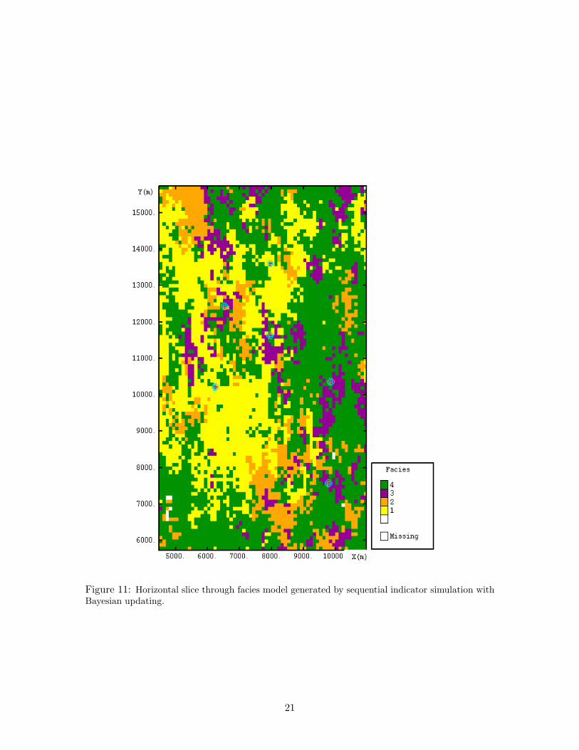
Figure 11: Horizontal slice through facies model generated by sequential indicator simulation withBayesian updating.

21

Figure 12: Cross section through facies model generated by sequential indicator simulation withBayesian updating.

22

Figure 13: Horizontal slice through facies model generated by sequential indicator simulation withBlock cokriging.

23

Figure 14: Cross section through facies model generated by sequential indicator simulation withBlock cokriging.

24