1

CS 188: Artificial Intelligence

Fall 2010

Lecture 21: Speech / ML

11/9/2010

Dan Klein – UC Berkeley

Announcements

� Assignments:

� Project 2: In glookup

� Project 4: Due 11/17

� Written 3: Out later this week

� Contest out now!

� Reminder: surveys (results next lecture)

2

Contest!

3

Today

� HMMs: Most likely explanation queries

� Speech recognition

� A massive HMM!

� Details of this section not required

� Start machine learning

4

Speech and Language

� Speech technologies� Automatic speech recognition (ASR)

� Text-to-speech synthesis (TTS)

� Dialog systems

� Language processing technologies� Machine translation

� Information extraction

� Web search, question answering

� Text classification, spam filtering, etc<

HMMs: MLE Queries

� HMMs defined by� States X

� Observations E

� Initial distr:

� Transitions:

� Emissions:

� Query: most likely explanation:

XX2

E1

X1 X3 X4

E2 E3 E4 E

6

2

State Path Trellis

� State trellis: graph of states and transitions over time

� Each arc represents some transition

� Each arc has weight

� Each path is a sequence of states

� The product of weights on a path is the seq’s probability

� Can think of the Forward (and now Viterbi) algorithms as

computing sums of all paths (best paths) in this graph

sun

rain

sun

rain

sun

rain

sun

rain

7

Viterbi Algorithm

sun

rain

sun

rain

sun

rain

sun

rain

8

Digitizing Speech

9

Speech in an Hour

� Speech input is an acoustic wave form

s p ee ch l a b

Graphs from Simon Arnfield’s web tutorial on speech, Sheffield:

http://www.psyc.leeds.ac.uk/research/cogn/speech/tutorial/

“l” to “a”

transition:

10

� Frequency gives pitch; amplitude gives volume

� sampling at ~8 kHz phone, ~16 kHz mic (kHz=1000 cycles/sec)

� Fourier transform of wave displayed as a spectrogram

� darkness indicates energy at each frequency

s p ee ch l a b

Spectral Analysis

11

Part of [ae] from “lab”

� Complex wave repeating nine times� Plus smaller wave that repeats 4x for every large cycle

� Large wave: freq of 250 Hz (9 times in .036 seconds)

� Small wave roughly 4 times this, or roughly 1000 Hz

12

[ demo ]

3

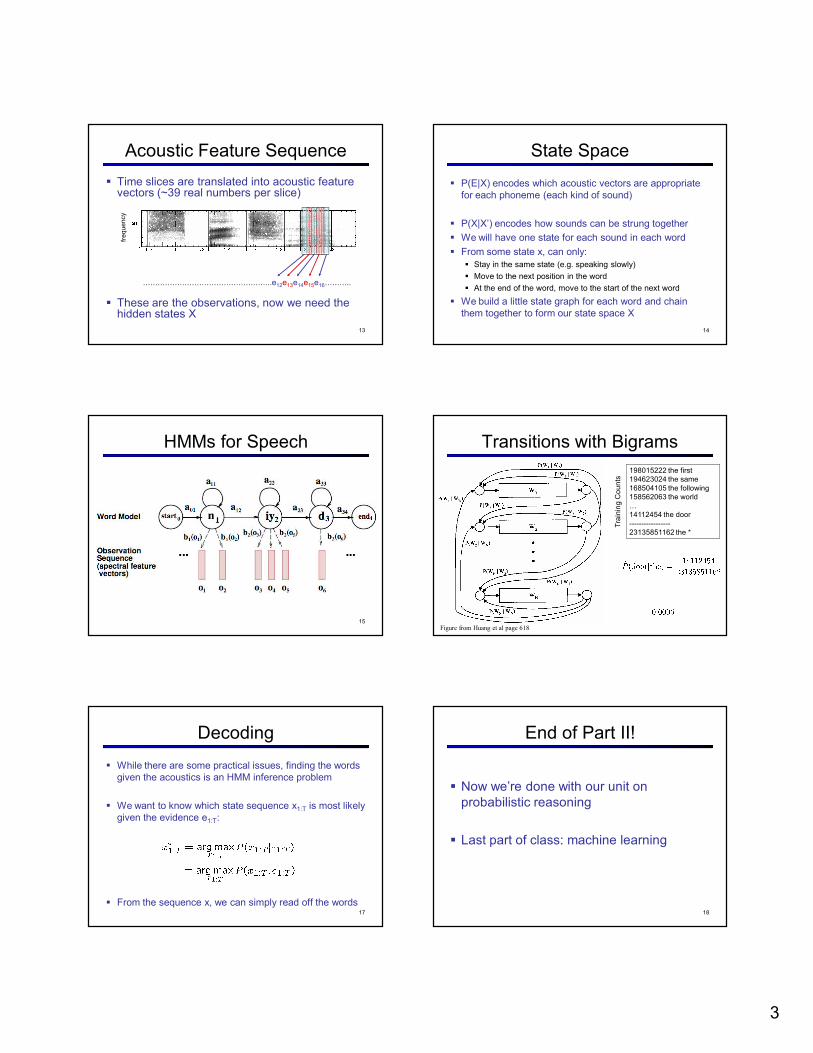
Acoustic Feature Sequence

� Time slices are translated into acoustic feature vectors (~39 real numbers per slice)

� These are the observations, now we need the hidden states X

<<<<<<<<<<<<<<<<<..e12e13e14e15e16<<<..

13

State Space

� P(E|X) encodes which acoustic vectors are appropriate

for each phoneme (each kind of sound)

� P(X|X’) encodes how sounds can be strung together

� We will have one state for each sound in each word

� From some state x, can only:

� Stay in the same state (e.g. speaking slowly)

� Move to the next position in the word

� At the end of the word, move to the start of the next word

� We build a little state graph for each word and chain

them together to form our state space X

14

HMMs for Speech

15

Transitions with Bigrams

Figure from Huang et al page 618

198015222 the first

194623024 the same

168504105 the following

158562063 the world

<

14112454 the door

-----------------

23135851162 the *

Tra

inin

g C

ou

nts

Decoding

� While there are some practical issues, finding the words

given the acoustics is an HMM inference problem

� We want to know which state sequence x1:T is most likely

given the evidence e1:T:

� From the sequence x, we can simply read off the words17

End of Part II!

� Now we’re done with our unit on

probabilistic reasoning

� Last part of class: machine learning

18

4

Machine Learning

� Up until now: how to reason in a model

and how to make optimal decisions

� Machine learning: how to acquire a model

on the basis of data / experience

� Learning parameters (e.g. probabilities)

� Learning structure (e.g. BN graphs)

� Learning hidden concepts (e.g. clustering)

Parameter Estimation

� Estimating the distribution of a random variable

� Elicitation: ask a human (why is this hard?)

� Empirically: use training data (learning!)� E.g.: for each outcome x, look at the empirical rate of that value:

� This is the estimate that maximizes the likelihood of the data

r g g

r g g

r gg

rg

g

r gg

r

g

g

Estimation: Smoothing

� Relative frequencies are the maximum likelihood estimates

� In Bayesian statistics, we think of the parameters as just another random variable, with its own distribution

????

Estimation: Laplace Smoothing

� Laplace’s estimate:

� Pretend you saw every outcome

once more than you actually did

� Can derive this as a MAP

estimate with Dirichlet priors (see

cs281a)

H H T

Estimation: Laplace Smoothing

� Laplace’s estimate (extended):� Pretend you saw every outcome

k extra times

� What’s Laplace with k = 0?

� k is the strength of the prior

� Laplace for conditionals:� Smooth each condition

independently:

H H T