External reference pricing policies, price controls, andinternational patent protection

Difei Geng∗ and Kamal Saggi†

Department of EconomicsVanderbilt University

September 2015

Abstract

We develop a two-country model to analyze how a country’s external referencepricing (ERP) policy affects the international availability and pricing of a patentedproduct sold by a local firm. In equilibrium, the country permits a level of interna-tional price discrimination that is just necessary to induce its firm to export and thispolicy maximizes joint welfare. By raising the minimum price above which the firmprefers to export, the ERP policy undermines the foreign price control (PC). Thereexist circumstances where tightening the PC is Pareto-improving. International co-operation is necessary to ensure that instituting patent protection abroad increaseswelfare.

Keywords: External reference pricing policies, price controls, exporting, tradebarriers, patent protection, imitation, welfare. JEL Classifications: F10, F12, O34,D42.

∗E-mail: difei.geng.1@vanderbilt.edu.†E-mail: k.saggi@Vanderbilt.Edu.

1

1 Introduction

Governments across the world utilize a variety of policies to combat the market power

of firms selling patented pharmaceutical products. Two such commonly used policies are

external reference pricing (ERP) and price controls. Under a typical ERP policy, the price

that a country permits the seller of a patented product to charge in its market depends upon

its prices in a well-defined set of foreign countries, commonly called its reference basket.

For example, Canada’s ERP reference basket includes France, Germany, Italy, Sweden,

Switzerland, the UK and the USA while that of France includes Germany, Italy, Spain,

and the UK. Furthermore, while some countries — such as France and Spain —permit a

seller to charge only the lowest price in its reference basket, others —such as Canada and

Netherlands —are willing to accept either the average or the median price in their reference

baskets. In a recent report, the World Health Organization (WHO) notes that 24 of 30

OECD countries and approximately 20 of 27 European Union countries use ERP, with the

use being mostly restricted to on-patent medicines (WHO, 2013).

Price controls on pharmaceuticals come in various shapes and forms: for example, gov-

ernments may control the ex-manufacturer price, the wholesale markup, the pharmacy

margin, the retail price, or use some combination of these measures. While few, if any,

countries use all such measures, many use at least some of them. For example, Kyle (2007)

notes that price controls in the pharmaceutical market are common in most major Euro-

pean countries where governments are fairly involved in the health-care sector. Similarly,

many developing countries have a long history of imposing price controls on patented phar-

maceuticals, many of which tend to be supplied by foreign multinationals. For example,

India has been imposing price controls on pharmaceuticals since 1962 and, despite the

existence of a robust domestic pharmaceutical industry, it recently chose to significantly

expand the list of drugs subject to price controls.1

This paper addresses several inter-related questions pertaining to ERP policies: What

are the underlying economic determinants of such policies? What type of international

spillovers do they generate? What are their overall welfare effects? Does their use by one

country reduce or increase the effectiveness of price controls in other countries? How does

the degree of patent protection in foreign markets affect a country’s ERP policy? What

are the effects of strengthening patent protection when both types of price regulations are

1See “India Widens Price Control over Medicines”in Wall Street Journal, May 17, 2013 and “Govern-ment Notifies New Drug Price Control Order”in the Indian Express, May 17, 2013.

2

endogenously determined?

We address these questions in a simple model with two countries (home and foreign)

where a single home firm produces a patented good, that it potentially sells in both markets.

The firm enjoys monopoly status at home by virtue of its patent; whether or not it faces

competition abroad depends upon the patent protection policy of the foreign country. The

home market is assumed to have more consumers and a greater willingness to pay for the

patented product, which in turn creates an incentive for the firm to price discriminate in

favor of foreign consumers. The home government sets its ERP policy —defined as the ratio

of the firm’s domestic price to its foreign price — in order to maximize national welfare,

which equals the sum of the firm’s global profit and domestic consumer surplus.

From the firm’s perspective, home’s ERP policy is a constraint on the degree of in-

ternational price discrimination that it is allowed to practice while from the domestic

government’s perspective it is a tool for lowering the price at home (while simultaneously

raising it abroad).2 While the home government internalizes the effects of its ERP policy

on local consumers and the firm, it does not take into account the negative effect on foreign

consumers. Since the domestic market is more lucrative for the firm, too tight an ERP

policy at home creates an incentive for the firm to not sell abroad so that it can sustain

its optimal monopoly price in the home market. This is an important mechanism in our

model and there is substantial empirical support for the idea that the use of ERP policies

on the part of rich countries can deter firms from serving low-price markets. For example,

using data from drug launches in 68 countries between 1982 and 2002, Lanjouw (2005)

shows that price regulations and the use of ERP by industrialized countries contributes

to launch delay in developing countries. Similarly, in their analysis of drug launches in

15 European countries over 12 different therapeutic classes during 1992-2003, Danzon and

Epstein (2008) find that the delay effect of a prior launch in a high-price EU country on a

subsequent launch in a low-price EU country is stronger than the corresponding effect of a

prior launch in a low-price EU country.3

In our two-country framework, while the firm only cares about its total global profit,

2In this sense, ERP policies are related to exhaustion policies that determine whether holders of IPRsare subject to competition from parallel imports or not. Unlike ERP policies. the economics of exhaustionpolicies has been investigated widely in the literature: see Malueg and Schwarz (1994), Richardson (2002),Li and Maskus (2006), Valletti (2006), Grossman and Lai (2008), and Roy and Saggi (2012).

3Further evidence consistent with launch delay spurred by the presence of price regulations is providedby Kyle (2007) who uses data on 1444 drugs produced by 278 firms in 134 therapeutic classes from 1980-1999 to study the pattern of drug launches in 21 countries.

3

home welfare also depends on the source of those profits, i.e., it matters whether profits

come at the expense of domestic or foreign consumers. We find that in equilibrium, the

home government sets its ERP policy at a level at which the firm is just willing to export.

Furthermore, the more asymmetric is demand across countries or the higher are foreign

trade barriers, the more lax is home’s ERP policy.

Since home’s ERP policy tends to induce the firm to raise its foreign price, we extend the

core model to allow the foreign government to impose a price control in order to curtail the

international spillover caused by home’s ERP policy. An important result of this analysis

is that home’s ERP policy undermines the foreign price control since the minimum price

at which the home firm is willing to sell abroad is higher when home has an ERP policy in

place relative to when it does not.

If the two countries simultaneously choose their respective policies, there exist a contin-

uum of equilibria: essentially any pair of policies that makes the firm indifferent between

selling only at home and selling in both markets constitutes a Nash equilibrium. For ex-

ample, a scenario where home allows unrestricted international price discrimination (i.e.

uses no ERP policy at all) and foreign sets its price control equal to marginal cost is an

equilibrium. But so is an outcome where home sets its ERP policy at a level that is op-

timal in the absence of a price control abroad and, in equilibrium, foreign refrains from

imposing any price control. An interesting point is that even if the foreign price control is

set exactly at the firm’s optimal monopoly price p∗F for that market, home’s equilibrium

ERP policy ends up being more lax relative to the case where the foreign price control is

completely absent. The intuition for this result is that when there exists no price control

abroad, home’s optimal ERP policy actually causes the equilibrium foreign price (p∗c) to

exceed the firm’s optimal monopoly price p∗F for that market (i.e. p∗c > p∗F ). As a result,

in the presence of an endogenously chosen ERP policy at home, a price control set at p∗Factually binds for the firm.4

A rather surprising insight of our model is that a tightening of the foreign price control

can raise welfare in both countries. The intuition for this result is as follows. Whenever

p∗c > p∗F a reduction in the foreign price (i.e. a tightening of the price control) increases

the firm’s foreign profit even as it reduces its domestic profit due to the foreign price

control spilling over to the home country via its ERP policy. For price controls in the

range [p∗F , p∗C ], if the foreign country tightens its price control only a moderate adjustment

4This result supports Goldberg’s (2010) intuitive argument that the use of ERP policies on the part ofdeveloped countries has the potential to generate significant negative spillovers for developing countries.

4

in home’s ERP policy is required to ensure that the firm continues to export since foreign

profits actually increase when the foreign price declines. Thus, due to home’s ERP policy,

not only does the foreign price control generate an international spillover, the nature of

the spillover generated is such that a tightening of the foreign price control can even make

both countries better off.

Price controls are not the only means for combating the market power of foreign firms

selling patented and/or branded pharmaceuticals: to some extent governments can also

lower local prices by weakening patent protection and promoting local generic production.

However, there are several problems with this strategy. First, the quality of generic pro-

duction can be subpar, especially in developing countries. Second, if a country encourages

generic production by allowing imitation of a pharmaceutical product that is under patent

in other countries, it can run afoul of existing multilateral rules and disciplines pertaining

to the protection of intellectual property specified in the Agreement on Trade Related As-

pects of Intellectual Property (TRIPS) that was ratified by the World Trade Organization

(WTO) in 1995 and is binding upon all existing WTO members. Indeed, international

frictions over widespread imitation of patented pharmaceuticals and various copyrighted

products by firms in many developing countries were a major driver of TRIPS. Accordingly,

we examine the implications of the degree of patent protection available to the firm abroad

and show that the lack of such protection induces the home country to loosen its ERP pol-

icy. This result fits well with the observation that when choosing the reference basket for

their ERP policies, most EU countries tend to include other EU countries that have similar

levels of patent protection. Finally, we show that some degree of international cooperation

—over either home’s ERP policy or over foreign’s price control or both —is necessary for

ensuring that joint welfare increases due to the strengthening of foreign patent protection.

By explicitly bringing in international pricing considerations and policy interaction

between national governments, our paper contributes to the rapidly developing literature

on the economics of internal reference pricing policies, i.e. policies under which drugs

are clustered according to some equivalence criteria (such as chemical, pharmacological, or

therapeutic) and a reference price within the same market is established for each cluster.

Brekke et. al. (2007) analyze three different types of internal reference pricing in a model

of horizontal differentiation where two firms sell brand-name drugs while the third firm sells

a generic version, that like in our model, is perceived to be of lower quality.5 They compare

5See Gislandi (2011) for an analysis where insured consumers pay the difference between the price ofa drug and the reference price R set by the regulator and generic producers can potentially collude to

5

generic and therapeutic reference pricing —with each other and with the complete lack of

reference pricing —and show that the latter type of reference pricing generates stronger

competition and lower prices. In similar spirit, Miraldo (2009) compares two different

reference pricing policies in a two-period model of horizontal differentiation: one where

reference price is the minimum of the observed prices in the market and another where it

is a linear combination of those prices. In the model, the reference pricing policy of the

regulator responds to the first period prices set by firms (which, in turn, the firms take

into account while setting their prices). The key result is that consumer surplus and firm

profits are lower under the "linear policy" since the first period price competition between

firms is less aggressive under this policy.

Bardey et. a. (2010) analyze a model in which firms choose to invest in research and

development (R&D) prior to negotiating prices with a regulator. In their model, reference

pricing affects the bargaining game between an innovator that brings a new drug to the

market and the regulator in the following way: if there are two drugs in a therapeutic class

then consumers (i.e. patients) are reimbursed only the lower price in that class.6 They

show that the presence of reference pricing dampens R&D incentives.

Motivated by the Norwegian experience, Brekke et. al. (2011) provide a comparison

of domestic price caps and reference pricing on competition and welfare and show that

whether or not reference pricing is endogenous —in the sense of being based on market prices

as opposed to an exogenous benchmark price —matters a great deal since the behavior of

generic producers is markedly different in the two scenarios; in particular, generic producers

have an incentive to lower their prices when facing an endogenous reference pricing policy

in order to lower the reference price, which in turn makes the policy preferable from the

viewpoint of consumers.7 Using a panel data set covering the 24 most selling off-patent

molecules, they also empirically examine the consequences of a 2003 policy experiment

where a sub-sample of off-patent molecules was subjected to reference pricing, with the

rest remaining under price caps. They find that prices of both brand names and generics

fell due to the introduction of reference pricing while the market shares of generics increased.

determine the level of R.6As an extension of our core analysis, in section 5 of the paper we derive the home country’s optimal

ERP policy when the firm’s foreign price is determined by Nash bargaining between the firm and theforeign government.

7The price cap regulation Norway is an ERP policy where the reference basket is the following set of‘comparable’countries: Austria, Belgium, Denmark, Finland, Germany, Ireland, the Netherlands, Sweden,and the UK. Unlike us, Brekke et. al. (2011) focus on the domestic market and take foreign prices to beexogenously determined.

6

The rest of this paper is structured as follows. We first introduce our two-country

framework and analyze the optimal ERP policy of the home country as well as its welfare

implications. Next, in section 3, we allow the foreign country to impose a price control

and study interaction between home’s ERP policy and the foreign price control. In section

4, we consider the interaction between these policies under a scenario where the foreign

country does not offer patent protection so that the home firm faces competition from

generic producers in (only) the foreign market. Here, we also examine the consequences of

forcing the foreign country to offer patent protection to the home firm. In section 5, we

extend the model to a scenario where the foreign price is determined by bargaining between

the firm and the foreign government. Section 6 concludes while section 7 constitutes the

appendix.

2 A benchmark model of ERP

We consider a world comprised of two countries: home (H) and foreign (F ). There is a

single home firm who sells a product (x) with a quality level s. The product is patented

in both markets. Consumer in country i (i = H,F ) buys at most 1 unit of the good at

local price pi. The number of consumers in country i equals ni. If a consumer buys the

good, her utility is given by ui = st−pi, where t measures the consumer’s taste for quality.Utility under no purchase equals zero and the quality parameter s is normalized to 1. For

simplicity, t is assumed to be uniformly distributed over the interval [0, µi] where µi ≥ 1.From the firm’s viewpoint, the two markets differ due to three underlying reasons.8

First, home consumers value quality relatively more, that is, µH = µ ≥ 1 = µF . Second,

the home market is larger: nH = n ≥ 1 = nF . Third, trade is subject to barriers/transport

costs where 0 ≤ b < 1 denotes the ad-valorem foreign trade barrier facing the firm’s exports.

As one might expect, given these conditions, the firm has an incentive to price discriminate

internationally.

The home government sets an external reference pricing (ERP) policy that stipulates

the maximum price ratio that its firm can set across countries. In particular, let pH and

pF be prices in the home and foreign markets respectively given that the firm sells in both

countries. Then, home’s ERP policy requires that the firm’s pricing abide by the following

8We later extend the model to allow for a foreign price control and for the imperfect protection ofintellectual property abroad. Both of these features are highly relevant in the context of the pharmaceuticalindustry, which is where ERP policies occur most commonly.

7

constraint:

pH ≤ δpF

where δ ≥ 1 reflects the rigor of home’s ERP policy. A more stringent ERP policy corre-sponds to a lower δ which gives the firm less room for international price discrimination.

Due to the assumed structure of demand in the two countries, the firm would never want

to discriminate in favor of home consumers so there is no loss of generality in assuming

δ ≥ 1. Note also that when δ = 1 the firm does not have any room to price discriminate

across markets.

2.1 Pricing under the ERP constraint

If the ERP constraint is absent altogether, the firm necessarily sells in both markets since

doing so yields higher total profit than selling only at home. In particular, when the firm

can freely chooses prices across countries, it sets a market specific price in each country to

maximize its global profit as follows

maxpH , pF

π(pH , pF ) ≡n

µpH(µ− pH) +

pFτ(1− pF ) (1)

where τ = 1/(1−b) > 1. It is straightforward to show that the firm’s optimal market specificprices are given by p∗H = µ/2 and p∗F = 1/2. The associated sales in each market equal

x∗H = n/2 and x∗F = 1/2. Global sales under price discrimination equal x∗ = x∗H + x∗F =

(n+ 1)/2. Observe that

p∗H/p∗F = µ ≥ 1

i.e. from the firm’s viewpoint, the optimal degree of international price discrimination

equals µ. Let the firm’s global profit under optimal monopoly prices be denoted by π∗ ≡π(p∗H , p

∗F ).

Now consider the firm’s pricing problem when facing the ERP constraint pH ≤ δpF .

Since µ is the maximum price differential the firm charges across markets, in the core model

we can restrict attention to δ ≤ µ without loss of generality.9 Of course, we implicitly

assume that the government has the ability to sustain whatever degree of international

price discrimination that it chooses to permit (i.e. any price differentials that arise cannot

be undercut via arbitrage by third parties).

9It is worth pointing out here that our model embeds two frequently utilized market structures ininternational trade, i.e. those of perfect market integration and segmentation, with the former scenariocorresponding to δ = 1 and the latter to δ = µ.

8

When faced with the ERP constraint, the firm can either choose to sell only at home

and thereby free itself of the ERP constraint or sell in both markets and abide by it, in

which case it solves:10

maxπ(pH , pF ) subject to pH ≤ δpF

Given a binding ERP constraint, the firm’s optimal prices when it sells in both markets

are

pδH =µδ(nτδ + 1)

2(nτδ2 + µ)and pδF = pδH/δ (2)

The sales associated with these prices can be recovered from the respective demand curves

in the two markets and these equal

xδH =δ2 + (2µ− δ)n2(δ2 + µn)

and xδF =n(2δ2 + (n− δ)µ2(δ2 + µn)

Global sales under the ERP constraint equal xδ = xδH + xδF . Using the above formulae,

it is straightforward to show the following:

Lemma 1: Provided the firm sells in both markets, its global sales when facing an ERP

policy at home exceed those under unrestricted international price discrimination:

xδ − x∗ = n(δ − 1)(µ− δ)2(nδ2 + µ)

≥ 0.

Observe from lemma 1 that when the firm is allowed no room to price discriminate (i.e.

δ = 1) then total sales under the ERP constraint are the same as those under price dis-

crimination, i.e. xδ = x∗. As we will see below, Lemma 1 has important implications for

the global welfare effects of home’s ERP policy.

Using the prices pδH and pδF , the firm’s global profit πδ = π(pδH , p

δF ) when facing the

ERP constraint is easily calculated

πδ = π(pδH , pδF ) =

µ(nτδ + 1)2

4τ(nτδ2 + µ)(3)

As one might expect,∂πδ

∂δ> 0

for 1 ≤ δ ≤ µ, that is, the firm’s global profit increases as home’s ERP policy becomes

looser.10Within the context of our model, any foreign price that exceeds the choke off price abroad (i.e. pF ≥ 1)

is tantamount to the firm not exporting since no foreign consumers are willing to buy the good if pF ≥ 1.

9

Of course, the firms always has the option to escape the ERP constraint by eschewing

exports altogether. If it does so, it collects the optimal monopoly profit π∗H in the home

market where

π∗H =n

µp∗H(µ− p∗H) = nµ/4 (4)

Since (i) ∂πδ/∂δ > 0; (ii) πδ∣∣δ≥µ = π∗ > π∗H ; and (iii) π

∗H is independent of δ, we can solve

for the critical ERP policy above which the firm prefers to sell in both markets relative to

selling only at home. We have:

πδ ≥ π∗H ⇐⇒ δ ≥ δ∗ where δ∗ ≡ 12

[µ− 1

nτ

](5)

We refer to δ∗ as the export inducing ERP policy. The first main result can now be

stated:

Proposition 1: When facing the ERP constraint pH ≤ δpF the firm exports if and only

if the ERP policy is less stringent than the export inducing ERP policy δ∗ (i.e. δ ≥ δ∗).

Given that the firm exports (i.e. δ ≥ δ∗), the following hold:

(i) home’s ERP policy reduces the local price relative to the optimal monopoly price

whereas it raises the foreign price: pδH ≤ p∗H and pδF ≥ p∗F ;

(ii) the home price decreases in the stringency of home’s ERP policy (i.e. ∂pδH/∂δ > 0

for 1 ≤ δ ≤ µ) whereas the foreign price increases in it: ∂pδF/∂δ < 0;

(iii) prices in both markets increase if foreign trade barriers increase (i.e. ∂pδi/∂τ > 0),

the home market gets larger (i.e. ∂pδi/∂n > 0), or if home consumers start to value the

product more (i.e. ∂pδi/∂µ > 0).

Proof : see appendix.

Part (i) says that the introduction of an ERP policy at home makes domestic consumers

better off at the expense of foreign consumers. It is worth noting that home’s ERP policy

induces the firm to raise its price above its optimal monopoly price p∗F in the foreign market

since it wants to avoid lowering the price in the more lucrative domestic market too much.

Along the same lines, given that an ERP policy is in place at home and the firm exports,

a decrease in the stringency of this policy (i.e. an increase in δ) makes foreign consumers

better off. Thus, the use of an ERP policy by the home country generates a negative

international spillover for foreign consumers, a theme to which we return below when

analyzing the optimal ERP policy from a joint welfare perspective.

Observe that the export inducing ERP policy δ∗ is increasing in all three basic para-

meters of the model (i.e. µ, n, and τ) since an increase in any of these parameters makes

10

the home market relatively more profitable for the firm thereby making it more reluctant

to export under the ERP constraint. As a result, the more lucrative the home market, the

greater the room to price discriminate that the firm requires in order to prefer selling in

both markets to selling only at home.

2.2 Optimal ERP policy

Having understood the firm’s pricing and export behavior, we are now in a position to

derive the home country’s optimal ERP policy. To do so, we assume that the objective

of the home country is to maximize its national welfare, i.e., the sum of local consumer

surplus and total profit of the firm:

wH(pH , pF ) = csH(pH) + π(pH , pF ) (6)

where csH(pH) denotes consumer surplus in the home market and it equals

csH(pH) =n

µ

µ∫pH

(t− pH)dt

An ERP policy is attractive for the home country since it can help reduce the deadweight

loss associated with monopoly pricing (see part (i) of Proposition 1). On the other hand,

too strict a ERP policy can induce the firm to eschew exports altogether, an outcome

under which home consumers fare the same as they do in the complete absence of an ERP

policy whereas the firm fares strictly worse (since it makes no export profit). Thus, for any

ERP policy for which the firm does not export, the home country is strictly better off not

imposing any ERP constraint on the firm. On the other hand, provided the firm exports,

home welfare increases with a decline in domestic price which calls for a tighter ERP policy.

We can directly state the main result:

Proposition 2: Let µ∗ ≡ 2+1/nτ . The optimal ERP policy of the home country is δe

where

δe =

{1 if µ ≤ µ∗

δ∗ otherwise

Observe that for µ > µ∗, home’s optimal ERP policy permits some degree of interna-

tional price discrimination (i.e. δe = δ∗ > 1) whereas for µ ≤ µ∗ it calls for the firm to

set a common international price (i.e. δe = 1).11 The logic behind this result is simple. In

11It is worth noting here that Proposition 2 continues to describe the Nash equilibrium if the homecountry and the firm were to make their decisions simultaneously.

11

terms of home welfare, discouraging the firm from exporting is even worse than not having

an ERP policy whatsoever, as in both cases the firm makes monopoly profit π∗H in the

home market, but only in the latter case does the firm export and also collect monopoly

profit π∗F in the foreign market. In general, the firm cares only about its total profit and

not where it comes from. By contrast, the home government also cares about the source of

that profit so that the firm’s export incentive is too weak relative to what is domestically

optimal. The optimal ERP policy of the home government ensures that the firm does not

refrain from exporting just so that it can charge its optimal monopoly price at home.

While our model abstracts from any fixed cost of exporting, it is worth noting that

Proposition 2 continues to even hold if the firm must bear a fixed cost ϕ prior to exporting.

Then, given the home country’s ERP policy, the firm exports iff

πδ − ϕ ≥ π∗H ⇐⇒ ϕ ≤ ϕ∗(δ) ≡ πδ − π∗H =µ(2nδ + 1− nµ)4(δ2n+ µ)

where ϕ∗(δ = δ∗) = 0 and ϕ∗(δ = µ) = π∗F . Observe that if ϕ > π∗F , the firm does not

export even if it can perfectly price discriminate across countries. Since ∂ϕ∗(δ)/∂δ > 0 for

all δ ≤ µ the function ϕ∗(δ) can be inverted to obtain the minimum value of δ, denoted

by δe(ϕ), above which the firm is willing to export. Given this, for ϕ ∈ [0, π∗F ] the homecountry’s optimal ERP policy is once again to allow just enough price discrimination to

induce the firm to export, i.e., δ∗(ϕ) = δe(ϕ), where δe(ϕ = 0) = δ∗ and ∂δe(ϕ)/∂ϕ > 0.12

The logic is same as before: setting a policy more lax than δe(ϕ) lowers domestic welfare

because it increases the firm’s total profit at the expense of domestic consumers while

setting a policy more stringent than δe(ϕ) leads the firm to not sell abroad.

Proposition 2 has substantial empirical support. When defining the set of foreign coun-

tries whose prices are used to determine the local price that a firm is allowed to charge,

countries typically tend to include foreign countries with similar market sizes and per capita

incomes.13 In particular, we do not observe EU countries setting ERP policies on the basis

of prices in low income developing countries. If lowering local prices were the sole moti-

vation of ERP policies, European governments would have an incentive to use the lowest

available foreign prices while setting their ERP policies. The insight provided by our model

12For ϕ > π∗F , home country’s ERP policy is irrelevant since the firm does not export for any ERPpolicy.13Observe also that home’s optimal ERP policy becomes less stringent as foreign trade barriers increase.

Once again, this result corresponds quite well with the nature of ERP policies observed in the real world.For example, the set of countries that inform the ERP policies of a typical EU country tend to be otherEU countries and trade within the EU is essentially subject to no policy barriers.

12

is that they do not do so because casting too wide a net while setting ERP policies can

backfire by causing local firms to forsake foreign markets just so that they can sustain high

prices in their domestic markets. In our model, demand size considerations are captured by

parameters n and µ and home’s optimal ERP policy becomes more lax with an increase in

either of these parameters. Setting the ERP policy in this fashion is necessary for ensuring

that the firm chooses to sell in both markets as opposed to selling only in its domestic

market (at the monopoly price p∗H).

Given that home’s ERP policy affects the firm’s export incentive as well as the price it

sets abroad, we now investigate the properties of the jointly optimal ERP policy.

2.3 Joint welfare

Let joint welfare be defined by:

w(pH , pF ) ≡ wH(pH , pF ) + csF (pF ) where csF =

1∫pF

(t− pF )dt

The jointly optimal ERP policy maximizes

maxδ

w(pH , pF ) subject to pH ≤ δpF

We first state the result and then explain its logic:

Proposition 3: Home’s nationally optimal ERP policy δe also maximizes joint welfare.

Proposition 3 is rather surprising since it argues that home’s (subgame perfect) Nash

equilibrium ERP policy is effi cient in the sense of maximizing aggregate welfare even though

home chooses its policy without taking into account its effects on foreign consumers. We

now explain the logic behind this result.

An effi cient ERP policy has to balance two objectives. One, it has to lower the interna-

tional price differential as much as possible since the existence of such a differential implies

that the marginal consumer in the high-price country values the last unit sold more than

the marginal consumer in the low-price country so reallocating sales towards the high-price

country raises welfare. Two, the ERP policy must ensure that foreign consumers have

access to the good. For µ ≤ µ∗, the firm exports even when it must charge the same price

in both markets so that it is optimal to fully eliminate the international price differential

(i.e. set δ = 1). For µ > µ∗, incentivizing the firm to export requires that it be given some

leeway to price discriminate internationally.

13

To see why δ∗ maximizes joint welfare when µ > µ∗, simply note that starting at δ∗

lowering δ (i.e. making the ERP policy more stringent) reduces foreign welfare to zero

since the firm does not export while it also reduces home welfare since domestic price

increases from pδH to p∗H while the firm’s profit remains unchanged (i.e. it equals π∗H).

Thus, implementing an ERP policy that is more stringent than δ∗ results in a Pareto-

inferior outcome relative to δ∗.

Now consider increasing δ above δ∗. At δ = δ∗ if the home’s ERP policy is relaxed (i.e.

δ is raised) the firm continues to export but increases its price at home while lowering it

abroad. Thus, starting at δ∗, an increase in δ makes the foreign country better off while

making the home country worse off. Indeed, from the foreign country’s viewpoint it would

be optimal to eliminate the ERP constraint since that yields the lowest possible price in its

market (i.e. p∗F ). However, since the international price differential increases with δ (i.e.

pδH/pδF = δ), joint welfare declines in δ for all δ > δ∗. In fact, given that the firm sells in

both markets, we can show directly that

∂w

∂δ=nµ(δ − µ)(nδ + 1)4(nδ2 + µ)2

< 0 for δ < µ.

Thus, it is jointly optimal to lower the international price differential as much as possible

while simultaneously ensuring that foreign consumers do not lose access to the patented

product. This is exactly what the home country’s Nash equilibrium ERP policy δe accom-

plishes.

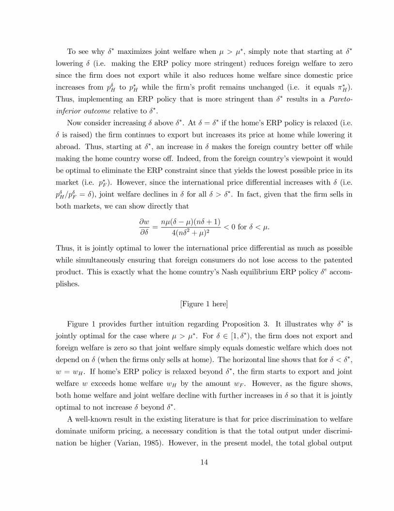
[Figure 1 here]

Figure 1 provides further intuition regarding Proposition 3. It illustrates why δ∗ is

jointly optimal for the case where µ > µ∗. For δ ∈ [1, δ∗), the firm does not export and

foreign welfare is zero so that joint welfare simply equals domestic welfare which does not

depend on δ (when the firms only sells at home). The horizontal line shows that for δ < δ∗,

w = wH . If home’s ERP policy is relaxed beyond δ∗, the firm starts to export and joint

welfare w exceeds home welfare wH by the amount wF . However, as the figure shows,

both home welfare and joint welfare decline with further increases in δ so that it is jointly

optimal to not increase δ beyond δ∗.

A well-known result in the existing literature is that for price discrimination to welfare

dominate uniform pricing, a necessary condition is that the total output under discrimi-

nation be higher (Varian, 1985). However, in the present model, the total global output

14

of the firm under price discrimination is actually lower than that which it produces when

facing an ERP constraint (Lemma 1). As a result, it is jointly optimal to restrain price

discrimination to the lowest level that is necessary for ensuring that foreign consumers do

not go unserved.

In our benchmark model, the foreign country’s government plays no role. In the real

world, governments frequently impose price controls on patented pharmaceuticals in order

to improve consumer access. Furthermore, in the context of our model, the use of an ERP

policy generates a negative price spillover for the foreign country and therefore creates a

natural incentive for a price control. We now allow the foreign country to directly control

the price in its market in order to study interaction between home country’s ERP policy

and the foreign country’s price control. Through-out the rest of the paper, we assume that

there is suffi cient asymmetry between markets that the home’s optimal ERP policy allows

some degree of discrimination (i.e. µ > µ∗ so that δe = δ∗).

3 ERP policy with a foreign price control

While price controls can take various forms, we model the foreign price control in the

simplest possible manner: the foreign country directly sets the patented product’s price

(pc) in its market. For expositional ease, through-out the rest of the paper we set τ = 1

(i.e. no trade barriers). Since the foreign country is a pure consumer of the patented good,

its objective is to secure access to the good at the lowest possible price. If home does not

impose an ERP policy, it is optimal for the foreign country to set the price control equal to

the firm’s marginal cost (i.e. pc = 0). In the absence of an ERP policy at home, the firm is

willing to export for any foreign price greater than or equal to its marginal cost, and this

allows the foreign country to impose its most desirable price control. It follows then that

since the existence of an ERP policy at home causes the foreign price control to partly spill

over to the home market thereby making the firm more reluctant to export, home’s ERP

policy undermines the effectiveness of the foreign price control.

3.1 Policy interaction and the firm’s decision

To fully explore the nature of interaction between home’s ERP policy and the foreign

country’s price control, we now analyze the following two-stage game:

Stage 1: home country chooses its ERP policy δ while the foreign country simultane-

15

ously sets its local price control pc.

Stage 2: firm chooses its domestic price pH .

If the firm chooses to export, it sets pH to maximize aggregate profit while being subject

to an ERP policy at home and a price control abroad:

maxpH ≤ δpc

n

µpH(µ− pH) + pc(1− pc) where pc ∈ [0, 1] (7)

Assuming that the ERP constraint pH ≤ δpc binds, the solution to the above problem

requires the firm to set pH = δpc so that its total profit equals:14

πδ(pc) =n

µ

δpcµ(µ− δpc) + pc(1− pc) (8)

In other words, when the firm faces an ERP policy at home and a price control abroad,

it essentially has no freedom to choose prices if it opts to export: it charges pc abroad and

δpc at home. If the firm chooses not to export, it charges its optimal monopoly price at

home and earns π∗H . Thus, when facing a price control abroad and an ERP policy at home,

the firm exports iff

πδ(pc) ≥ π∗H (9)

This inequality yields the export inducing ERP policy as a function of the foreign price

control:15

δ(pc) =µ

2pc−√ηµpc(1− pc)2ηpc

(10)

Note that in the complete absence of policy intervention, the firm would charge its

monopoly price p∗F in the foreign market, which serves as the natural upper bound for pc in

the absence of an ERP policy at home. However, when an ERP policy is in place at home

and it binds, the foreign price exceeds the monopoly level (i.e. pδF ≥ p∗F ). Thus, in the

presence of an ERP policy at home, the natural upper bound for the foreign price control

is the choke-off price pc = 1.

Lemma 2: (i) ∂δ(pc)/∂pc < 0 for 0 < pc < p∗c where p∗c ≡ pδF (δ

∗) = nµ/(1 + nµ) and

limpc→0

δ(pc) =∞.

14It will turn out that in any Nash equilibrium of the policy game, the ERP constraint necessarily binds.15Observe that the ERP constraint necessarily binds so long as p∗H ≥ δpc which is the same as δ ≤

δb(pc) ≡ p∗H/pc. Now observe that the ERP policy that induces exporting can be written as δ(pc) =p∗H/pc −α(pc) where α(pc) ≡

√ηµpc(1− pc)/(2ηpc) ≥ 0. Therefore, δ(pc) ≤ δb(pc) which implies that the

export inducing ERP policy binds.

16

(ii) ∂δ(pc)/∂pc ≥ 0 for p∗c ≤ pc ≤ 1 with ∂δ(pc)/∂pc = 0 for pc = p∗c .

(iii) ∂2δ(pc)/∂p2c ≥ 0 for 0 ≤ pc ≤ 1.(iv) δ(p∗F ) > δ∗.

Proof : see appendix.

The first part of Lemma 2 says that if the foreign price control lies in the interval

0 ≤ pc < p∗c a tightening of the price control requires the home country to relax its ERP

policy if the firm is to continue to export. When pc < p∗c , the foreign price control is below

the firm’s optimal price pδF (δ∗) for the foreign market. A tighter price control lowers the

firm’s global profit under exporting, so the home’s ERP policy has to be relaxed to offset

the negative effect on the firm’s incentive to export.

This result is noteworthy since it shows that, over the range 0 ≤ pc < p∗c , the foreign

price control generates an international spillover by undermining the home country’s ability

to implement its most desirable ERP policy. Indeed, δ(pc) tends to infinity as pc falls to

zero: an extremely stringent price control (pc ≈ 0) translates into a zero home price for anyfinite δ, so that there exists no ERP policy that can provide the firm suffi cient incentive to

export.

The second part of Lemma 2 highlights a region (i.e. p∗c ≤ pc ≤ 1) where home’s

ERP policy actually becomes tighter as the foreign price control becomes more stringent.

When pc ≥ p∗c , the foreign price control is above the firm’s optimal price for the foreign

market.16 Thus, a tightening of the price control actually increases the firm’s incentive

to export which in turn allows the home country to tighten its ERP policy. Thus, when

p∗c ≤ pc ≤ 1, prices in both countries fall if the foreign price control becomes tighter. Sincethe firm’s total profit remains unchanged (i.e. continues to equal π∗H) while consumers in

both countries gain from a reduction in pc, it is Pareto improving to lower pc as long as

p∗c ≤ pc. Finally, the third inequality of Lemma 2 says that δ(pc) is convex in pc, indicating

that the home’s ERP policy must adjust to a larger extent as the price control abroad

becomes stricter. This property of δ(pc) plays an important role in determining the jointly

optimal pair of policies, an issue that we address in section 2.1 below.

Part (iv) of Lemma 2 points out that even if the foreign price control is set at the firm’s

optimal monopoly price (i.e. pc = p∗F ) for that market, the home country’s ERP policy is

more lax than the export inducing policy in the absence of a price control. The intuition

for this is that in the absence of a foreign price control, the home country’s optimal ERP

16We show below that such a price control can indeed arise in Nash equilibrium.

17

policy actually causes the foreign price to exceed the firm’s optimal monopoly price (i.e.

pδF (δ∗) > p∗F ) for that market so that, in the presence of an endogenous ERP policy in the

home country, a foreign price control set at p∗F actually binds for the firm.

3.2 Equilibrium

It is clear that, given pc, the optimal ERP for the home country is the export inducing policy

δ(pc). We now characterize the foreign country’s optimal price control given a certain ERP

policy in the home country. If the firm does not export, the foreign country has no access to

the good and its welfare equals zero. Moreover, conditional on the firm exporting, a more

lax price control policy is counter-productive as it simply raises the local price. Hence,

for a given ERP policy, the foreign country picks the lowest possible price control that

just induces the firm to export. For pc ∈ [0, p∗c ] since the δ(pc) function is monotonicallydecreasing in pc, its inverse pc(δ) yields the best response of the foreign country to a given

ERP policy of the home country. For pc ∈ [p∗c , 1] since the δ(pc) function is increasing inpc, there exist two possible price controls that yield the firm the same level of global profit

for any given ERP policy. However, since it is optimal for the foreign country to pick the

lower of these two price controls, the best response of the foreign country can never exceed

p∗c . Thus, pc(δ) is strictly decreasing in δ so that foreign’s best response curve coincides

with the downward sloping part of the δ(pc) curve. This implies that all points to left of

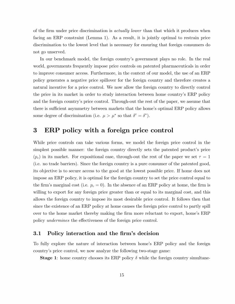
p∗c on the δ(pc) curve (plotted in Figure 2) constitute a Nash equilibrium.

[Figure 2 here]

We can state the following:

Proposition 4: Any pair of export inducing policies {pc, δ} where pc ≤ p∗c and δ ≥ δ∗

constitutes a Nash equilibrium. In all Nash equilibria, the firm’s global profit equals π∗H .

For Nash equilibria in which pc ∈ [0, p∗F ], the home price declines in the foreign price control(i.e. ∂pδH(pc)/∂pc = ∂[δ(pc)pc]/∂pc < 0) whereas for Nash equilibria in which pc ∈ [p∗F , p∗c ],it increases with it (i.e. ∂pδH(pc)/∂pc ≥ 0).17 Furthermore, pδH(pc → 0) = p∗H .

18

17It is worth noting that there also exist Nash equilibria where the foreign country’s equilibrium pricecontrol lies above the optimal monopoly price for its market. Obviously, this happens when the home setsa very stringent ERP policy so that a high price in the foreign market is necessary to induce the firm toexport.18As pc → 0 the home price converges to the monopoly price p∗H because the home country is forced to

completely drop its ERP policy (i.e. δ∗(pc) tends to +∞) when pc → 0.

18

Proposition 4 says that when the foreign price control is lax (i.e. p∗F < pc ≤ p∗c), a

tightening of the foreign price control (i.e. a reduction in pc) lowers the home price through

the adjustment of home’s ERP policy whereas when the price control is relatively stringent

(pc ≤ p∗F ), a further decline in pc raises the home price. The response of home’s ERP

policy to changes in the foreign price control (described in Proposition 4) is crucial to

understanding the non-monotonicity of pδH(pc). To see why, note that

∂pδH(pc)

∂pc= δ(pc) + pc

∂δ(pc)

∂pc(11)

so that if ∂δ(pc)/∂pc ≥ 0 then the home price would necessarily increase with the foreignprice control since δ(pc) > 0. However, as Lemma 2 notes ∂δ(pc)/∂pc < 0 whenever

0 < pc < p∗c , i.e., for this range of the foreign price control, the home country tightens its

ERP policy as the foreign price control relaxes. This adjustment in the home’s ERP policy

tends to reduce the home price pδH . Next, note that since ∂2δ(pc)/∂p

2c ≥ 0, the home’s ERP

policy adjusts to a larger extent when the foreign price control is stricter. Indeed, we can

see this more directly by considering the elasticity of home’s ERP policy with respect to

the foreign price control, which is defined as

εδ ≡ −∂δ(pc)

∂pc

pcδ

Observe that∂pδH(pc)

∂pc≤ 0⇐⇒ εδ ≥ 1 (12)

It is straightforward to show that

εδ ≥ 1 iff pc ≤ p∗F (13)

As a result, the home price declines in pc for all pc ∈ (0, p∗F ] whereas it increases with it forpc ∈ (p∗F , p∗c).We have shown that policy interaction between the two countries leads to multiple Nash

equilibria that lie along the downward sloping part of the δ(pc) curve. We now show that

these equilibria have different welfare properties.

3.3 Welfare

Recall that the firm’s total profit does not play a role in the welfare analysis, since in any

Nash equilibrium the firm’s profit equals its monopoly profit under no exporting (π∗H), i.e.,

19

the firm is indifferent between selling only at home and selling in both markets. This is

a convenient property which allows us to focus on each country’s consumer surplus when

discussing welfare. We directly state the main result and then explain its logic:

Proposition 5:

(i) For all Nash equilibria in which pc ∈ (p∗F , p∗C ] tightening the foreign price control(i.e. reducing pc) makes both countries better off.

(ii) For pc ∈ (0, p∗F ], reductions in pc make the foreign country better off at the expenseof the home country.

(iii) There exists a unique pair of policies {δw, pwc } that maximizes joint welfare, where

pwc < p∗F and δw > δ∗.

Figure 2 is useful for explaining the logic of Proposition 5. This figure plots the δ(pc)

curve in (pc, δ) space. The equilibrium in the absence of a foreign price control is given

by point A1 in Figure 2 the coordinates of which are (p∗c , δ). To understand the intuition

behind Proposition 5 first consider the case where pc ∈ (p∗F , p∗c ]. Over this range, a reductionin the foreign price requires the home country to make its ERP policy less stringent (∂δ(pc)

∂pc<

0) to ensure that the firm’s export incentive is preserved. But since δ(pc)∂pc

is relatively small

in magnitude in this region, the direct decline in pc dominates the increase in δ(pc) so that

pδH(pc) = δ(pc)pc declines as pc falls. Thus, both countries gain from a tighter foreign price

control when pc ∈ (p∗F , p∗c ].When pc ∈ (0, p∗F ], any further reductions in the foreign price control require a sharp

increase in the home’s ERP policy in order to preserve the firm’s export incentive. Here, a

tightening of the foreign price control increases the home price (due to the sharp adjustment

in its ERP policy) so that the home country loses while the foreign country gains from

reducing pc.

It is clear that a jointly optimal pair of policies must lie on the δ(pc) curve in Figure

2. Any combination of policies above this curve lowers welfare by creating an international

price differential while any policy pair below the curve has the same effect by inducing the

firm to not export. Furthermore, from the above discussion it is also clear that any jointly

optimal price control has to lie in the range (0, p∗F ]. The jointly optimal pair of policies

solves the following problem

maxδ, pc

w(δpc, pc) (14)

Substituting δ(pc) into (14) and maximizing over pc yields the jointly optimal price

20

control:19

pwc = p∗F [1− θ(n, µ)] (15)

where

θ(n, µ) =1√

1 + nµ(16)

Observe thatp∗F − pwcp∗F

= θ(n, µ) (17)

Since 0 < θ(n, µ) ≤ 1, the jointly optimal price control is strictly smaller than the firm’smonopoly price for the foreign market (i.e. pwc < p∗F ). Indeed, θ(n, µ) measures the per-

centage reduction in the firm’s monopoly price abroad that is jointly optimal to impose.

Since θ(n, µ) is decreasing in n as well as µ, the more lucrative the firm’s domestic market

(i.e. the higher are n or µ), the less binding is the foreign price control. When either n or

µ become arbitrarily large, θ(n, µ) approaches 0 so that it becomes jointly optimal to let

the firm charge its monopoly price in the foreign market. The jointly optimal ERP policy

δw can be recovered by substituting pwc = pwc in equation (10). Since p∗c < p∗F we must

have δw > δ∗, i.e., the jointly optimal ERP policy in the presence of an optimally chosen

foreign price control is more lax than when the foreign price control is absent. Thus, the

foreign price control allows the home country to also implement a more desirable ERP

policy provided the two countries coordinate their policies.

3.4 Discussion: timing of moves

Since the time horizon for the implementation and adjustment of an ERP policy may not

be same as that for a price control, in this section we discuss alternative timing scenarios

where one of the countries moves first.

Suppose home can commit to an ERP policy before foreign chooses its price control.

It is clear that if home has the first move then it will choose its most preferred point on

the δ(pc) curve in Figure 2. From Proposition 5, this point is given by (p∗F , δ(p∗F )) and it is

denoted by pointH on Figure 2, which lies Southeast of the welfare maximizing policy pair

(pw, δw) denoted as pointW. The reason point H is home’s most preferred policy pair is

that home price pδH(pc) = δ(pc)pc declines in pc when pc ∈ (0, p∗F ] whereas it increases withit for pc ∈ (p∗F , p∗c) so that, subject to the firm exporting, home price is minimized at point19It is easy to verify that the second-order condition holds at p∗c .

21

H. Intuitively, since the firm has the strongest incentive to export when its foreign price

equals the optimal monopoly price p∗F , by choosing to implement the policy δ(p∗F ) home can

induce foreign to pick the price control p∗F . In the absence of a foreign price control, point

H is unattainable for home since if it were to announce the policy δ(p∗F ) the firm would

export and its price abroad would equal pδF (δ = δ(p∗F )) > p∗F and its total profit would

exceed π∗H . But when the foreign price control exists and responds endogenously to home’s

ERP policy, home can implement δ(p∗F ) knowing that foreign will impose the lowest price

consistent with the firm exporting, which equals p∗F . Thus, when it moves first, home is

able to utilize the foreign price control to obtain a level of welfare that cannot be achieved

in its absence.

Since the foreign price equals p∗F , from the viewpoint of foreign consumers the outcome

when home moves first coincides with that which obtains when the firm is completely free to

set its optimal prices in both markets. Even though the firm charges its optimal monopoly

price p∗F abroad when home implements δ(p∗F ), the ability of home to commit to an ERP

policy also makes foreign consumers better off relative to the case where there is no price

control because the foreign price under δ∗ is strictly higher than that under δ(p∗F ) (i.e.

p∗c > p∗F ).

Further note that δ(p∗F ) > δ∗: i.e. when it moves first, home’s most preferred ERP

policy in the presence of a foreign price control is more lax than its ERP policy when

there is no price control abroad. The intuition for this result is clear: absent the foreign

price control, the firm raises its price abroad to p∗c (which exceeds p∗F ) forcing home to set

a stricter ERP policy to keep the domestic price low while preserving the firm’s export

incentive.

Finally, observe that δ(p∗F ) < δw so that when moving first home selects an ERP policy

that is more stringent than the welfare maximizing policy δw because it ignores the effect

of its decision on foreign consumers.

Now suppose foreign selects the price control before home chooses its ERP policy. In

such a scenario, foreign would set its price control equal to the marginal cost of production

(i.e. pc ' 0) knowing that home will then impose no ERP policy on the firm in order to

induce it to export. Price at home would then equal the optimal monopoly price p∗F . Thus,

the outcome when foreign chooses the price before home chooses its ERP policy coincides

with that which obtains when home has no ERP policy in place at all.

22

4 Lack of patent protection abroad

We now extend the model to a scenario where the home firm’s patent is not protected

abroad. As in Saggi (2013), the lack of foreign patent protection is assumed to result in

the establishment of a competitive generic industry that produces a product whose quality

equals γ where γ ∈ [0, 1]. The larger is γ, the closer is the perceived quality of the genericto that of the patented good so that γ captures the intensity of generic competition faced

by the firm. Since the generic industry is competitive in nature, the price of the generic

equals its marginal cost of production (which equals zero). Note, however, that since the

firm’s patent is protected at home, generic sales are limited to the foreign market.

4.1 Foreign patent protection and home’s ERP policy

Given a price p for the firm’s patented product, foreign consumers can be partitioned into

two groups: those in the range [0, th(p; γ)] buy the low quality whereas those in [th(p; γ), 1]

buy the high quality where th(p; γ) = p/(1 − γ) defines the marginal consumer who is

indifferent between the patented good and the generic. If not constrained by government

policies, the patent-holder chooses its price p to maximize

maxπI(p; γ) = p[1− th(p; γ)]

which yields the firm’s profit maximizing price when facing generic competition as

p∗F (γ) = (1− γ)/2 = (1− γ)p∗F

We first investigate how the home country’s optimal ERP policy changes due to the

lack of patent protection abroad. When facing the ERP policy constraint pH ≤ δpF (γ), if

the firm sells in both markets it solves

maxpH , pF

π(pH , pF ; γ) =n

µpH(µ− pH) + pF (1−

pF1− γ ) subject to pH ≤ δpF

which yields the optimal prices as

pδH(γ) =µδ(nδ + 1)(1− γ)2[nδ2(1− γ) + µ]

and pδF (γ) = pδH(γ)/δ (18)

It is straightforward to shown that

∂pδH∂γ

< 0 and∂pδF∂γ

< 0

23

That is, given that the firm sells in both markets when facing an ERP policy at home,

generic competition abroad lowers prices in both markets, with the home price falling due

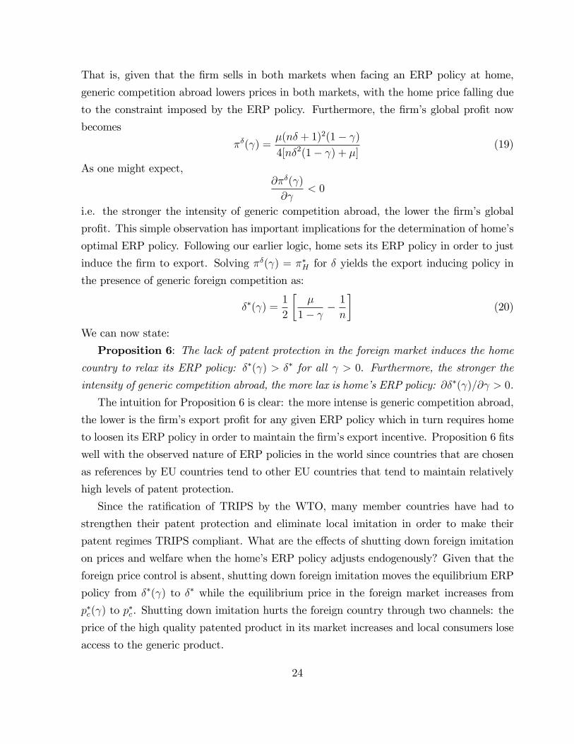
to the constraint imposed by the ERP policy. Furthermore, the firm’s global profit now

becomes

πδ(γ) =µ(nδ + 1)2(1− γ)4[nδ2(1− γ) + µ]

(19)

As one might expect,∂πδ(γ)

∂γ< 0

i.e. the stronger the intensity of generic competition abroad, the lower the firm’s global

profit. This simple observation has important implications for the determination of home’s

optimal ERP policy. Following our earlier logic, home sets its ERP policy in order to just

induce the firm to export. Solving πδ(γ) = π∗H for δ yields the export inducing policy in

the presence of generic foreign competition as:

δ∗(γ) =1

2

[µ

1− γ −1

n

](20)

We can now state:

Proposition 6: The lack of patent protection in the foreign market induces the home

country to relax its ERP policy: δ∗(γ) > δ∗ for all γ > 0. Furthermore, the stronger the

intensity of generic competition abroad, the more lax is home’s ERP policy: ∂δ∗(γ)/∂γ > 0.

The intuition for Proposition 6 is clear: the more intense is generic competition abroad,

the lower is the firm’s export profit for any given ERP policy which in turn requires home

to loosen its ERP policy in order to maintain the firm’s export incentive. Proposition 6 fits

well with the observed nature of ERP policies in the world since countries that are chosen

as references by EU countries tend to other EU countries that tend to maintain relatively

high levels of patent protection.

Since the ratification of TRIPS by the WTO, many member countries have had to

strengthen their patent protection and eliminate local imitation in order to make their

patent regimes TRIPS compliant. What are the effects of shutting down foreign imitation

on prices and welfare when the home’s ERP policy adjusts endogenously? Given that the

foreign price control is absent, shutting down foreign imitation moves the equilibrium ERP

policy from δ∗(γ) to δ∗ while the equilibrium price in the foreign market increases from

p∗c(γ) to p∗c . Shutting down imitation hurts the foreign country through two channels: the

price of the high quality patented product in its market increases and local consumers lose

access to the generic product.

24

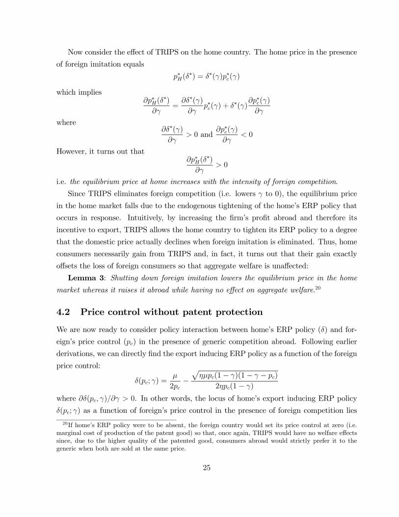
Now consider the effect of TRIPS on the home country. The home price in the presence

of foreign imitation equals

p∗H(δ∗) = δ∗(γ)p∗c(γ)

which implies∂p∗H(δ

∗)

∂γ=∂δ∗(γ)

∂γp∗c(γ) + δ∗(γ)

∂p∗c(γ)

∂γ

where∂δ∗(γ)

∂γ> 0 and

∂p∗c(γ)

∂γ< 0

However, it turns out that∂p∗H(δ

∗)

∂γ> 0

i.e. the equilibrium price at home increases with the intensity of foreign competition.

Since TRIPS eliminates foreign competition (i.e. lowers γ to 0), the equilibrium price

in the home market falls due to the endogenous tightening of the home’s ERP policy that

occurs in response. Intuitively, by increasing the firm’s profit abroad and therefore its

incentive to export, TRIPS allows the home country to tighten its ERP policy to a degree

that the domestic price actually declines when foreign imitation is eliminated. Thus, home

consumers necessarily gain from TRIPS and, in fact, it turns out that their gain exactly

offsets the loss of foreign consumers so that aggregate welfare is unaffected:

Lemma 3: Shutting down foreign imitation lowers the equilibrium price in the home

market whereas it raises it abroad while having no effect on aggregate welfare.20

4.2 Price control without patent protection

We are now ready to consider policy interaction between home’s ERP policy (δ) and for-

eign’s price control (pc) in the presence of generic competition abroad. Following earlier

derivations, we can directly find the export inducing ERP policy as a function of the foreign

price control:

δ(pc; γ) =µ

2pc−√ηµpc(1− γ)(1− γ − pc)

2ηpc(1− γ)where ∂δ(pc, γ)/∂γ > 0. In other words, the locus of home’s export inducing ERP policy

δ(pc; γ) as a function of foreign’s price control in the presence of foreign competition lies

20If home’s ERP policy were to be absent, the foreign country would set its price control at zero (i.e.marginal cost of production of the patent good) so that, once again, TRIPS would have no welfare effectssince, due to the higher quality of the patented good, consumers abroad would strictly prefer it to thegeneric when both are sold at the same price.

25

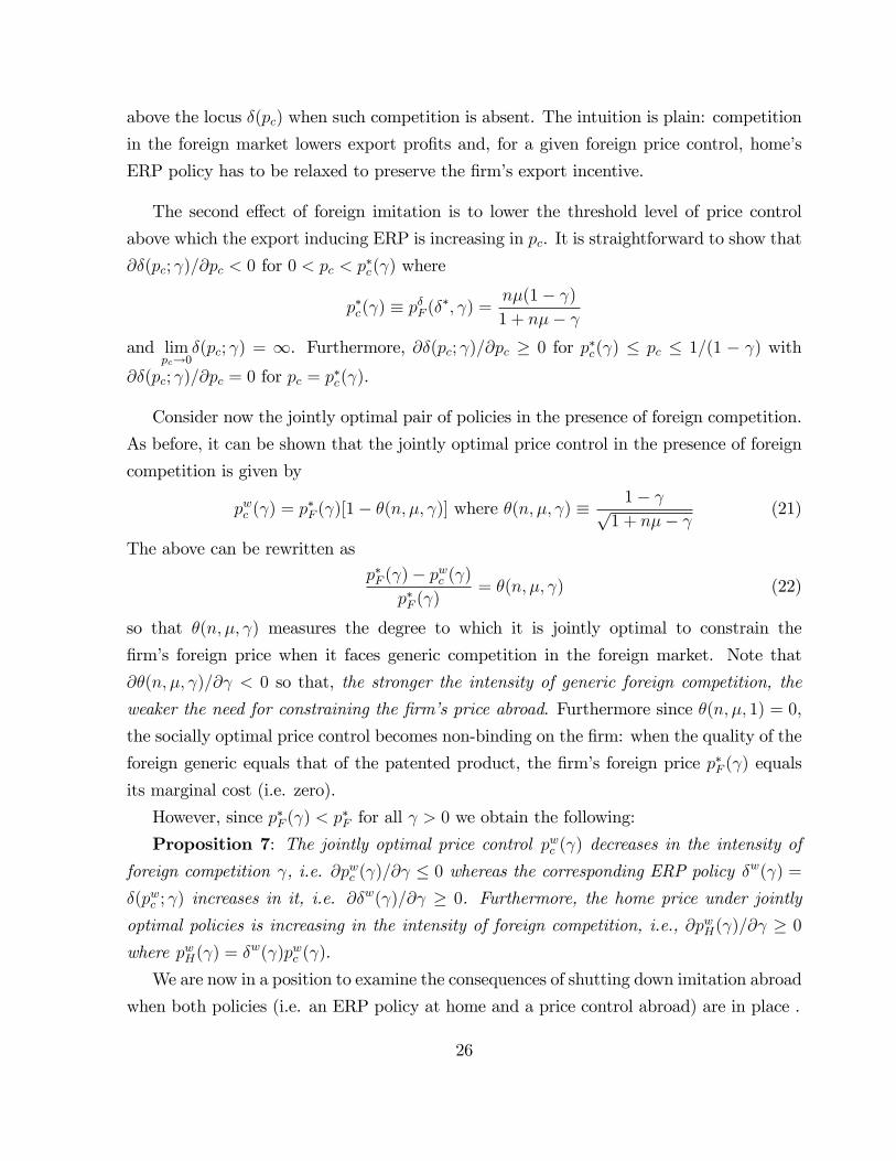
above the locus δ(pc) when such competition is absent. The intuition is plain: competition

in the foreign market lowers export profits and, for a given foreign price control, home’s

ERP policy has to be relaxed to preserve the firm’s export incentive.

The second effect of foreign imitation is to lower the threshold level of price control

above which the export inducing ERP is increasing in pc. It is straightforward to show that

∂δ(pc; γ)/∂pc < 0 for 0 < pc < p∗c(γ) where

p∗c(γ) ≡ pδF (δ∗, γ) =

nµ(1− γ)1 + nµ− γ

and limpc→0

δ(pc; γ) = ∞. Furthermore, ∂δ(pc; γ)/∂pc ≥ 0 for p∗c(γ) ≤ pc ≤ 1/(1 − γ) with

∂δ(pc; γ)/∂pc = 0 for pc = p∗c(γ).

Consider now the jointly optimal pair of policies in the presence of foreign competition.

As before, it can be shown that the jointly optimal price control in the presence of foreign

competition is given by

pwc (γ) = p∗F (γ)[1− θ(n, µ, γ)] where θ(n, µ, γ) ≡1− γ√

1 + nµ− γ (21)

The above can be rewritten as

p∗F (γ)− pwc (γ)p∗F (γ)

= θ(n, µ, γ) (22)

so that θ(n, µ, γ) measures the degree to which it is jointly optimal to constrain the

firm’s foreign price when it faces generic competition in the foreign market. Note that

∂θ(n, µ, γ)/∂γ < 0 so that, the stronger the intensity of generic foreign competition, the

weaker the need for constraining the firm’s price abroad. Furthermore since θ(n, µ, 1) = 0,

the socially optimal price control becomes non-binding on the firm: when the quality of the

foreign generic equals that of the patented product, the firm’s foreign price p∗F (γ) equals

its marginal cost (i.e. zero).

However, since p∗F (γ) < p∗F for all γ > 0 we obtain the following:

Proposition 7: The jointly optimal price control pwc (γ) decreases in the intensity of

foreign competition γ, i.e. ∂pwc (γ)/∂γ ≤ 0 whereas the corresponding ERP policy δw(γ) =δ(pwc ; γ) increases in it, i.e. ∂δ

w(γ)/∂γ ≥ 0. Furthermore, the home price under jointlyoptimal policies is increasing in the intensity of foreign competition, i.e., ∂pwH(γ)/∂γ ≥ 0where pwH(γ) = δw(γ)pwc (γ).

We are now in a position to examine the consequences of shutting down imitation abroad

when both policies (i.e. an ERP policy at home and a price control abroad) are in place .

26

4.3 If foreign country must offer patent protection

It is straightforward to show that if the domestic ERP policy and the foreign price control

were to remain fixed then the shutting down of foreign imitation makes home better off

by increasing the firm’s total profit while it lowers joint welfare by creating a deadweight

loss: foreign consumers lose access to the low quality good and their loss dominates the

firm’s gain. However, the effect of TRIPS when both home’s ERP policy and foreign’s price

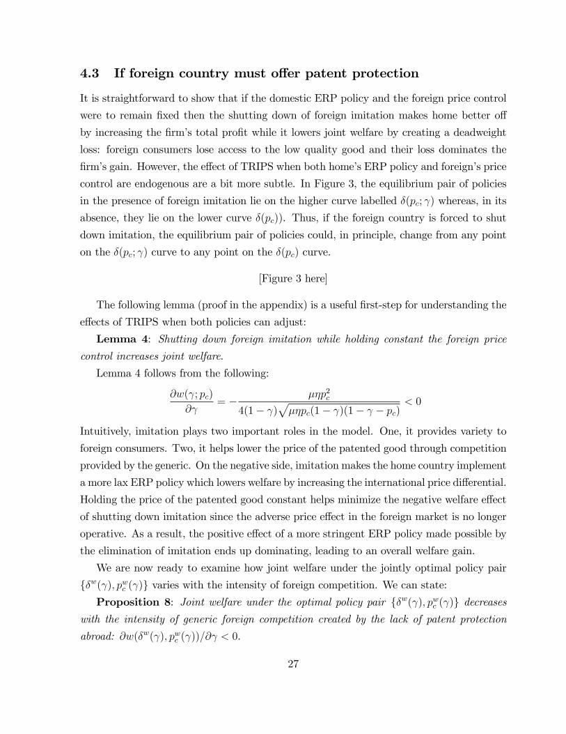
control are endogenous are a bit more subtle. In Figure 3, the equilibrium pair of policies

in the presence of foreign imitation lie on the higher curve labelled δ(pc; γ) whereas, in its

absence, they lie on the lower curve δ(pc)). Thus, if the foreign country is forced to shut

down imitation, the equilibrium pair of policies could, in principle, change from any point

on the δ(pc; γ) curve to any point on the δ(pc) curve.

[Figure 3 here]

The following lemma (proof in the appendix) is a useful first-step for understanding the

effects of TRIPS when both policies can adjust:

Lemma 4: Shutting down foreign imitation while holding constant the foreign price

control increases joint welfare.

Lemma 4 follows from the following:

∂w(γ; pc)

∂γ= − µηp2c

4(1− γ)√µηpc(1− γ)(1− γ − pc)

< 0

Intuitively, imitation plays two important roles in the model. One, it provides variety to

foreign consumers. Two, it helps lower the price of the patented good through competition

provided by the generic. On the negative side, imitation makes the home country implement

a more lax ERP policy which lowers welfare by increasing the international price differential.

Holding the price of the patented good constant helps minimize the negative welfare effect

of shutting down imitation since the adverse price effect in the foreign market is no longer

operative. As a result, the positive effect of a more stringent ERP policy made possible by

the elimination of imitation ends up dominating, leading to an overall welfare gain.

We are now ready to examine how joint welfare under the jointly optimal policy pair

{δw(γ), pwc (γ)} varies with the intensity of foreign competition. We can state:Proposition 8: Joint welfare under the optimal policy pair {δw(γ), pwc (γ)} decreases

with the intensity of generic foreign competition created by the lack of patent protection

abroad: ∂w(δw(γ), pwc (γ))/∂γ < 0.

27

This result has an important policy implication: if the two countries could jointly select

their respective policies and also decide whether or not to allow foreign imitation then

they would choose to not allow it (i.e. set γ = 0) and they would implement the policy

pair {δw, pwc }, i.e. they would prefer pointW1 on the δ(pc) curve to the pointW0 on the

δ(pc; γ) curve in Figure 3. However, even under such coordination, the foreign country loses

from eliminating imitation: not only does the price of the high quality product increase

in its market from pwc (γ) to pwc , its consumers also lose access to the low quality generic

product. The home country gains because the price in its market drops due to a tightening

of its ERP policy, which is also the reason that joint welfare increases.

Proposition 8 is supportive of TRIPS but it also rests on a degree of international

coordination that may not be always feasible. It is worth asking if there exist a less

stringent set of circumstances under which the elimination of generic foreign competition

can increase total welfare. This is particularly so because TRIPS does not involve any

international coordination over price controls or ERP policies.21 In this context, it is worth

noting that the welfare result in Proposition 8 would continue to hold even if the two

countries could coordinate their choices over patent protection abroad and only one of the

other two policies (i.e. home’s ERP policy or the foreign price control). To see why, suppose

the two countries coordinate their decisions over patent protection abroad and home’s ERP

policy, leaving the choice of the price control entirely in the hands of the foreign country.

Then, given that coordination precedes the setting of the price control, they can still attain

the welfare maximizing outcome by agreeing to implement patent protection abroad and

setting the home’s ERP policy at δw. Then, at the next stage, the foreign country would

find it optimal to select the price control pwc since this is the lowest price at which the firm

would choose to export. An analogous logic applies for the case where they coordinate over

patent protection and foreign’s price control, leaving the home free to set its own ERP

policy.

We now discuss the effects of TRIPS when policy coordination is completely absent.

The following result argues that in the absence of policy coordination, TRIPS has the

21While TRIPS does not explicitly mention ERP policies, Article 6 of TRIPS states that “nothing in thisAgreement shall be used to address the issue of the exhaustion of intellectual property rights.”Exhaustionpolicies are quite similar to ERP policies since they determine whether or not attempts at internationalprice discrimination on the part of holder of IPRs can be undone by the parallel trade across countries.Indeed, it appears that TRIPS essentially leaves countries free to use ERP policies and other price controlmeasures when these are deemed necessary for curtailing the market power enjoyed by holders of IPRs orfor achieving domestic objectives such as safeguarding public health by making necessary pharmaceuticalsmore widely available.

28

potential to increase aggregate welfare although it does not necessarily do so:

Proposition 9: Given an initial pair of policies {p0c , δ0} on the δ(pc; γ) curve, thereexists an interval of price controls [p1c , p

2c ] on the δ(pc) curve, where p

0c ∈ [p1c , p2c ], such that

welfare over [p1c , p2c ] is strictly higher than at {p0c , δ0}.

Figure 4 illustrates Proposition 9.

[Figure 4 here]

Suppose foreign imitation is allowed and let E0 ≡ {p0c , δ0} be the initial equilibriumpoint on the δ(pc; γ) curve such that p0c > pwc (which is greater than p

wc (γ)). If the foreign

country is forced to shut down imitation, the new equilibrium pair of policies could in prin-

ciple lie anywhere on the δ(pc) curve. Suppose, for the moment, that the new equilibrium

E1 on the δ(pc) curve lies vertically below E0 (i.e. the foreign price control remains fixed

at p0c). Then, from Lemma 4 it follows that welfare must be higher at E1 relative to E0.

Note also that, starting at E1, welfare declines as the foreign price control is increased

since we move further away from the welfare-maximizing foreign price pwc . Furthermore,

world welfare at points A0 and A1 is equal since these are cases where the foreign price

control is not binding (or missing) (see Lemma 2). Thus, we have

w(A0) = w(A1) < w(E0) < w(E1)

By continuity, there must exist a unique point E2 on the δ(pc) curve lying between E1

and A1 that yields the same welfare as point E0 on the δ(pc; γ) curve. Any pair of policies

between E1 and E2 on the δ(pc) curve yields strictly higher welfare than E0 on the δ(pc; γ)

curve. On the other hand, starting at point E1, as the price control is reduced along the

δ(pc) curve, we eventually hit a point E3 where the price control is so low that welfare at

E2 is the same as that at E0. We can be sure that E2 exists because at welfare at E0 is

strictly higher than it is at the limiting case where the price control equals zero. Thus, we

have shown that, given p0c > pwc , there exists a range of policy pairs without imitation that

yield higher welfare than the initial equilibrium E0 with imitation.22

4.4 Global generic competition

It is worth asking how our major conclusions change if the product sold by the firm is

off-patent so that it faces generic competition in both markets. This question is useful for22To avoid redundancy we do not discuss the cases where pwc (γ) < p0c < pwc or p

0c < pwc (γ). The arguments

for why Proposition 9 holds in these cases are analogous to those presented above.

29

examining whether and how the optimal ERP policy for products that are under patent

differs from those that are off patent.

Suppose the firm faces generic competition of quality γ in both markets.23 When the

product is not under patent, questions related to patent protection are moot. Consider then

the home’s optimal ERP policy when generic competition exists in both markets. Using

earlier derivations, the firm’s optimal monopoly prices in the two markets are p∗F (γ) =

(1 − γ)/2 and p∗H(γ) = µp∗F (γ). Using these prices and following previous derivations, it

is straightforward to show that the home country’s optimal ERP policy continues to be

defined by Proposition 2. This has an interesting implication: while the lack of patent

protection in only the foreign market forces home to weaken its ERP policy (Proposition

6), the lack of such protection in both markets (i.e. the product coming off patent given

that it has been protected in both markets) does not. Intuitively, in our model, generic

competition in both markets causes optimal prices to decline in both markets in a way that

its optimal degree of price discrimination does not change, i.e., p∗H(γ)/p∗F (γ) = p∗H/p

∗F = µ.

As a result, since the optimal ERP policy targets international price discrimination, it too

remains unaltered. For analogous reasons, we find that the jointly optimal price control

continues to be defined by equation (15) when generic competition exists in both markets.

5 Price bargaining

We now discuss the case where the price abroad is a result of bargaining between the

foreign government and the firm. The timing of moves is as follows. First, home chooses

its ERP policy. Next, the firm and the foreign government bargain over price. We utilize

the generalized Nash bargaining solution as the outcome of the bargaining subgame where

the firm’s payoffunder the disagreement point equals π∗H (i.e. its monopoly profit at home)

while that of the foreign government equals zero. We first discuss the case where the two

parties cannot use transfers or side payments and then the case where they can do so.

5.1 Bargaining without transfers

It is clear that, given the ERP policy set by home, the range of prices over which the firm

and the foreign government can find a mutually acceptable price is given by [pc(δ), pδF (δ)]

23In other words, we assume that the generic market is a single global market. It is straightforward toextend the model to allow for generic local competition in each country. To avoid redundancy, we do notdiscuss this case here.

30

where the pc(δ) is the foreign government’s most preferred price since it maximizes local

consumer surplus csF (p) (subject to the price being high enough to induce the firm to

export) whereas pδF (δ) is that of the firm since it maximizes its global profit πδ(p).

The price under Nash bargaining solves

maxp

β ln[csF (p)] + (1− β) ln[πδ(p; δ)− π∗h] (23)

where β ∈ [0, 1] can be interpreted as the bargaining power of the foreign governmentrelative to the firm. The first order condition for this problem is

β

csF (p)

dcsF (p)

dp+

1− βπδ(p; δ)− π∗h

dπδ(p; δ)

dp= 0

Using the relevant formulae, this first order condition can be rewritten as

2β

1− p =A(δ, p)(1− β)pA(δ, p)− nµ/4

where

A(δ, p) ≡ [(nδ + 1)− [2(nδ2 + µ)]p

µ]

It is straightforward to show that the solution to this equation is a price p(β, δ) ∈ [p(1, δ),p(0, δ)] where p(1, δ) = pc(δ); p(0, δ) = pδF (δ); and ∂p(δ, β)/∂β < 0.

Now consider home’s ERP policy decision. Home sets its ERP policy taking into account

the price p(δ, β) that emerges from the bargaining that follows. When β = 1, the home’s

ERP policy is given by point H in Figure 2. In this case, since the firm has zero bargaining

power, the foreign government effectively controls the price and the home’s most preferred

policy is set to ensure that the firm charges its optimal monopoly price abroad and therefore

has the strongest incentive to export. When β = 0, the firm is free to pick any price abroad

and home is able to set a much more stringent ERP policy and the equilibrium outcome

is denoted by point A1 in Figure 2. Observe that home is strictly better off when the

bargaining power lies totally in the hands of the foreign government relative to the case

where it lies with the firm. In fact, as argued earlier, total world welfare is also higher in

the former scenario. When bargaining power is split between the two parties, the firm earns

strictly positive rents in the bargaining subgame and p(δ, β) > pc(δ). At the first stage,

home simply chooses its most preferred point on this curve which will generally differ from

point A1.

31

5.2 If transfers can be used

Now consider the case where the firm and the foreign government can use transfers when

bargaining over price so that the foreign price is chosen to maximize the joint welfare of

the two parties.24 Thus, given home’s ERP policy, the foreign price is chosen to maximize

the sum of the firm’s global profit and consumer surplus abroad:

maxp

S(p) ≡ πδ(p) + csF (p)

It is straightforward to show that the solution to the above problem is

pb(δ) =nµδ

µ+ 2nδ2where 0 < pb(δ) < 1

Observe that pb(δ) is increasing in n and µ. As the home’s ERP policy becomes more

lax, it is optimal to lower the price abroad whereas when the home market becomes more

lucrative for the firm (either due to an increase in n or µ), the two parties agree to a higher

price in the foreign market. Furthermore, note that

∂pb(δ)

∂δ< 0 iff δ < δm ≡

õ

2n

The non-monotonicity of the jointly optimal foreign price pb(δ) in δ can be understood as

follows: when δ is small (i.e. near 1), the price in the home market is quite far from the

firm’s optimal home price so that its global profit is well below its maximum value. Starting

at δ ' 1, the jointly optimal foreign price pb(δ) increases in order to raise the firm’s profiteven though consumer surplus in the South declines. But once δ hits the threshold value of

δm, the jointly optimal foreign price decreases with δ because the relatively lax ERP policy

allows the firm to charge a fairly high price in the home market even though the foreign

price is low. Furthermore, note that pb(δ) goes to zero as δ approaches infinity — i.e. if

there is no ERP policy at home, the two parties agree to set price equal to marginal cost.

As before, we assume that the joint surplus is allocated between the two parties ac-

cording to the Nash bargaining rule. Under this rule, the firm’s payoff from bargaining

equals

πB = π∗H + (1− β)[S(pb(δ))− π∗H ]

while that of the foreign government equals

wBF = β[S(pb(δ))− π∗H ]24This assumption implies that the two parties can make side-payments to each other to ensure that the

jointly optimal price is charged in the foreign market.

32

where β ∈ [0, 1] represents the bargaining power of the foreign government.When setting its ERP policy, home takes into account that the firm will export iff its

payoff from doing so is at least as large as its domestic profit in the absence of exporting:

πB ≥ π∗H . Given that the firm exports, home welfare is decreasing in δ so that the home’s

most preferred ERP policy is one where the above inequality binds, which implies

(1− β)[S(pb(δ))− π∗H ] = 0

Solving this yields

δb =

√nµ(nµ− 2)2n

Proposition 10: Suppose the firm and the foreign government choose the foreign price

to maximize their joint welfare S(p). Then, regardless of how the total surplus is split

between the two parties, the home country’s optimal ERP policy is δb where ∂δb/∂µ > 0;

∂δb/∂n > 0; and δb < δ∗.

Several points are worth noting about the above result. First, since the home country

moves first, it is able to extract all of the surplus created by bargaining between its firm

and the foreign country by setting an ERP policy at which the total surplus available to

the two parties at their jointly optimal price equals the firm’s profit from not exporting

(i.e. S(pb(δ)) = π∗H). Second, the home country is able to implement a tighter ERP

policy when negotiations between the firm and the foreign country yield the effi cient price

pb(δ) as opposed to the profit-maximizing price pδF (δ) (i.e. δb < δ∗). Since total welfare

is decreasing in δ (conditional on the firm exporting), effi cient price negotiations increase

welfare by resulting in a more stringent ERP policy even though they make the foreign

country worse off relative to a situation where the price is chosen unilaterally by the firm.

Intuitively, when price is not negotiated, the home country is limited in its ability to extract

rent from the firm and the foreign country since, as argued earlier, the bargained price in

the absence of transfers must lie in the interval [(pc(δ), pδF (δ)] over the δ(pc) curve.

6 Conclusion

This paper sheds light on the economics of external reference pricing (ERP) and how

such a policy interacts with price controls abroad. We consider a model in which a single

firm sells a patented product in potentially two markets (home and foreign) where, owing

to differences in the structure of demand across countries, it has an incentive to price

discriminate in favor of foreign consumers.

33

We model home’s ERP policy as the degree to which the firm’s foreign price is allowed

to be lower than its domestic price and show that home’s optimal policy is to tolerate a

level of international price discrimination at which the firm is just willing to sell abroad. In

other words, the home country balances the interests of local consumers against the export

incentive of the firm. Intuitively, an ERP policy that is so stringent that it becomes profit

maximizing for the firm to not sell abroad in order to charge its optimal monopoly price

at home is never optimal for the home country. This result helps define the limits of ERP

policies and it suggests that countries with large domestic markets (such as the USA or

Germany) should use relatively less stringent ERP polices or else they can risk creating a

situation where their firms choose to not sell abroad just so that they can charge high prices

at home. We also show that an increase in foreign trade barriers induces the home country

to loosen its ERP policy. The practical implication of this result is that when defining

its reference basket, a country ought to pay closer attention to prices in geographically

proximate markets. As we noted earlier, real world ERP policies indeed seem to have this

characteristic.

Almost by design, home’s ERP policy generates a negative price spillover for foreign

consumers in our model. However, quite surprisingly, we find that the home country’s

optimal ERP policy maximizes aggregate welfare even though its sets the policy not taking

into account the interests of foreign consumers. Intuitively, since the home market is

larger and its consumers have a greater willingness to pay for the firm’s product, it is

jointly optimal to reduce international price discrimination to the lowest possible level

subject to the firm selling in both markets. This is exactly what home’s nationally optimal

ERP policy accomplishes in equilibrium. This result suggests that while ERP policies

create international price spillovers, their use does not necessarily create an argument for

international coordination. It is noteworthy in this regard that the TRIPS agreement of

the WTO is silent on the subject of ERP policies for patented products and it also leaves

member countries free to adopt exhaustion policies of their choosing, another type of policy

that creates international price spillovers via the flow of parallel trade across countries.

Another insight provided by the model is that home’s ERP policy reduces the effective-

ness of the foreign price control since it increases the minimum price at which the home

firm is willing to export. On the flip side, the presence of an ERP policy at home leads the

foreign price control to generate an international spillover for home consumers although

the nature of this spillover is not necessarily negative. Indeed, we demonstrate that there

34

exist circumstances where a tighter foreign price control raises welfare in both countries.

Furthermore, our welfare analysis shows that it is jointly optimal to restrict the firm’s for-

eign price below its optimal monopoly price for that market while simultaneously granting

it greater room to price discriminate internationally than the home country is willing to

provide in the absence of a price control abroad.

We also consider a scenario where the lack of patent protection abroad generates local

competition from a competitively priced generic version of the patented product. Such

competition induces the home country to implement a more lax ERP policy: since compe-

tition reduces foreign profits, the firm has to be given more room to price discriminate in

order for it to export. Finally, we show that some degree of international cooperation —over

either home’s ERP policy or over foreign’s price control or both —is necessary for ensuring

that joint welfare increases due to the strengthening of foreign patent protection. Absent

such cooperation, stronger patent protection abroad is not necessarily welfare-improving.

7 Appendix

Proof of Proposition 1

We first prove (ii). It can be shown that ∂pδH∂δ

= µ(2µnτδ−nτδ2+µ)2(nτδ2+µ)2

. Hence the sign of∂pδH∂δ

depends on the term 2µnτδ − nτδ2 + µ, which is always positive when δ ≥ δ∗. This

implies ∂pδH∂δ

> 0. As for the foreign price, we have ∂pδF∂δ

= −µnτ(nτδ2+2δ−µ)2(nτδ2+µ)2

and ∂pδF∂δ|δ∗ =

−2n2τ2µ(nτµ−3)(1+nτµ)3

. Since τ ≥ 1 > 3nµunder the assumption µ > 2 + 1

n, we have ∂pδF

∂δ|δ∗ < 0.

Moreover, ∂pδF

∂δ< 0 for δ ≥ δ∗ because ∂pδF

∂δis decreasing in δ.

To prove (i), first note that pδH |δ=µ = p∗H = µ2. As pδH increases in δ, we must have

pδH ≤ p∗H for 1 ≤ δ ≤ µ. As for the foreign price, note that ∂pδF∂δ

> 0 for 1 < δ < δ̂

and ∂pδF∂δ

< 0 for δ̂ < δ ≤ µ where δ̂ =√1+µnτ−1nτ

. This implies that pδF first increases

and then decreases in δ for 1 ≤ δ ≤ µ. Moreover, since pδF |δ=1 =µ(nτ+1)2(nτ+µ)

> p∗F =12and

pδF |δ=µ = p∗F =12, it follows that pδF ≥ p∗F for 1 ≤ δ ≤ µ.

To verify (iii), we directly calculate ∂pδH∂τ

= nµδ2(µ−δ)2(nτδ2+µ)2

> 0, ∂pδF∂τ

= nµδ(µ−δ)2(nτδ2+µ)2

> 0,∂pδH∂n= µτδ2(µ−δ)

2(nτδ2+µ)2> 0, ∂p

δF

∂n= µτδ(µ−δ)

2(nτδ2+µ)2> 0, ∂p

δH

∂µ= µτδ3(nτδ+1)

2(nτδ2+µ)2> 0 and ∂pδF

∂µ= µτδ2(nτδ+1)

2(nτδ2+µ)2> 0.

�Proof of Lemma 2

(i) We have ∂δ(pc)∂pc

= µ(pc−h(pc))2h(pc)p2c

, where h(pc) ≡√nµpc(1− pc). Observe that the sign

of ∂δ(pc)∂pc

depends on the term pc − h(pc). It is easy to check that pc − h(pc) < 0 when

35

0 < pc < p∗c , hence∂δ(pc)∂pc

< 0. Moreover, as pc −→ 0, both µ2pcand h(pc)

2ηpctend to infinity but

µ2pcconverges at a faster rate. Hence, we have lim

pc→0δ(pc) =∞.

(ii) By virtue of (i) as p∗c ≤ pc ≤ 1, pc − h(pc) ≥ 0 indicating ∂δ(pc)∂pc

≥ 0. Also,

substituting p∗c into∂δ(pc)∂pc

we obtain ∂δ(pc)∂pc|p∗c=0 = 0.

(iii) We have ∂2δ(pc)∂p2c

= µf(pc)4[h(pc)pc]3

where f(pc) ≡ nµp2c (4pc − 3) + 4(h3(pc)). It followsthat the sign of ∂2δ(pc)

∂p2cdepends on the sign of f(pc). To establish the result we need to

show that b(pc) > 0 for 0 < pc < 1. Note that f(pc)|pc=0 = 0 and f(pc)|pc=1 = ηµ > 0.

Moreover, using∂f(pc)

∂pc= 6nµ(1− 2pc)[h(pc)− pc]

it is easy to see that there exist two inflection points for f(pc) at pc = 12and pc = p∗c =

nµnµ+1

.

It can be shown that f(pc) > 0 at both these inflection points. Continuity of f(pc) implies

that we must have f(pc) > 0 for 0 < pc < 1 and therefore∂2δ(pc)∂p2c

> 0.

(iv) We have δ(p∗F )− δ∗ =nµ−2√nµ+1

2n> 0 because nµ > 3. �

Proof of Proposition 7

We have

∂pwc (γ)

∂γ= −2(1 + σ − γ)

√(1− γ)(1 + σ − γ)− 3σ(1− γ)− 2γ2 + 4γ − 24(1 + σ − γ)

√(1− γ)(1 + σ − γ)

where σ ≡ nµ. As the denominator of ∂pwc (γ)∂γ

is positive, to show that ∂pwc (γ)∂γ≥ 0 we only

need to show the numerator of ∂pwc (γ)∂γ

is positive.

Note that the numerator of ∂pwc (γ)∂γ

can be rewritten as

2(1 + σ − γ) 32√(1− γ)− 3σ(1− γ)− 2(1− γ)2

= 2(1 + σ − γ) 32√(1− γ)− (3σ + 2− 2γ)(1− γ)

As (1 − γ) ∈ [0, 1), we have√(1− γ) ≥ (1 − γ). Also note that σ ≡ nµ > 3 since by

assumption µ > 2+ 1n. Therefore we only need to show d(γ) > 0 for all σ > 3 and γ ∈ [0, 1)

where

d(γ) ≡ 2(1 + σ − γ) 32 − (3σ + 2− 2γ)

We have∂d(γ, σ)

∂σ= 3√1 + σ − γ − 3 > 0 for any σ ≥ 3

Therefore, as long as d(γ, σ) ≥ 0 at σ = 3, we know d(γ, σ) ≥ 0 for all σ > 3. To this end,note that

d(γ, σ)|σ=3 = 2(4− γ)32 − (11− 2γ)

36

is a decreasing function of γ because

∂(d(γ, σ)|σ=3)∂γ

= −3√4− γ + 2 < 0

Hence we can obtain the desirable result if d(γ, σ)|σ=3 ≥ 0 at γ = 1. This is indeed the

case since we have

d(γ, σ)|γ=1,σ=3 = 6√3− 9 > 0.

Now note that∂δw(γ)

∂γ=∂δw(γ)

∂pwc

∂pwc∂γ

We have already shown that ∂pwc∂γ

< 0. We must also have ∂δw(γ)∂pwc

< 0 due to the fact that

the ERP policy has to adjust to maintain suffi cient profits for the firm to export. This

completes the proof.

Finally, we can write∂pwH(γ)

∂γ=∂pwH(γ)

∂pwc

∂pwc∂γ

We know ∂pwH(γ)

∂pwc< 0 and similar reasoning to above yields the desired result (i.e. ∂pwH(γ)

∂γ≥ 0).

�

37

References

[1] Bardey David, Bommier Antoine and Jullien Bruno, 2010. “Retail Price Regulation

and Innovation: Reference Pricing in the Pharmaceutical Industry.”Journal of Health

Economics 29 (2), 303-316.

[2] Bond Eric W., Saggi Kamal, 2014. “Bargaining over Entry with a Compulsory License

Deadline: Price Spillovers and Surplus Expansion.”Mimeo, Vanderbilt University.

[3] Brekke Kurt R., Konigbauer Ingrid and Straume Odd R., 2007. “Reference Pricing of

Pharmaceuticals.”Journal of Health Economics 26, 613-642.

[4] Brekke Kurt R., Holmas Tor H. and Straume Odd R., 2011. “Reference Pricing, Com-

petition, and Pharmaceutical Expenditures: Theory and Evidence from a Natural

Experiment.”Journal of Public Economics 95, 624—638.

[5] Chaudhuri Shubham, Goldberg Pinelopi K. and Jia Panle, 2006. “Estimating the

Effects of Global Patent Protection in Pharmaceuticals: a Case Study of Quinolones

in India.”American Economic Review, 96 (5), 1477-1514.

[6] Cockburn Iain M., Lanjouw Jean O. and Schankerman Mark, 2014. “Patents and the

Global Diffusion of New Drugs.”NBER Working Paper 20492, Cambridge, MA.

[7] Danzon Patricia M., Epstein Andrew J., 2008. “Effects of Regulation on Drug Launch

and Pricing in Interdependent Markets.”National Bureau of Economic ResearchWork-

ing Paper No. 14041.

[8] Danzon Patricia M., Wang Richard Y. and Wang Liang, 2005. “The Impact of Price

Regulation on the Launch Delay of New Drugs.” Journal of Health Economics 14,

269-292.

[9] Gislandi Simone, 2011. “Competition and the Reference Pricing Scheme for Pharma-

ceuticals.”Journal of Health Economics 30, 1137-1149.

[10] Goldberg Pinelopi K., 2010. “Intellectual Property Rights Protection in Developing

Countries: the Case of Pharmaceuticals.”Journal of the European Economic Associ-

ation 8, 326-353.

38

[11] Grossman Gene M., Lai Edwin, 2008. “Parallel Imports and Price Controls.”Rand

Journal of Economics 39, 378-402.

[12] Ivus Olena, 2010. “Do Stronger Patent Rights Raise High-tech Exports to the Devel-

oping World?”Journal of International Economics 81, 38-47.

[13] Kanavos Panos, Costa-i-Font Joan, Merkur Sherry and Gemmill-Toyama Marin, 2004.

“The Economic Impact of Pharmaceutical Parallel Trade in European Member States:

a Stakeholder Analysis.”Special Research Paper, LSE Health and Social Care, London

School of Economics and Political Science.

[14] Kyle Margaret, 2007. “Pharmaceutical Price Controls and Entry Strategies.”The Re-

view of Economics and Statistics 89 (1), 88-99.

[15] Lanjouw Jean O., 2005. “Patents, Price Controls and Access to New Drugs: How

Policy Affects Global Market Entry.”National Bureau of Economic Research Working

Paper No. 11321.

[16] Li Changying, Maskus Keith E., 2006. “The Impact of Parallel Imports on Investments

in Cost- Reducing Research and Development.”Journal of International Economics

68 (2), 443-455.

[17] Malueg David A., Schwartz Marius, 1994. “Parallel Imports, Demand Dispersion, and

International Price Discrimination.”Journal of International Economics 37, 167-195.

[18] Maskus Keith E., 2000. “Parallel Imports.”World Economy 23, 1269-1284.

[19] Miraldo Marisa, 2009. “Reference Pricing and Firms’Pricing Strategies.”Journal of

Health Economics 28, 176—197.

[20] National Economic Research Associates (NERA), 1999. The Economic Consequences

of the Choice of Regime of Exhaustion in the Area of Trademarks. Final Report for

DG XV of the European Commission.

[21] Richardson Martin, 2002. “An Elementary Proposition Concerning Parallel Imports.”

Journal of International Economics 56, 233-245.

[22] Roy Santanu, Saggi Kamal, 2012. “Equilibrium Parallel Import Policies and Interna-

tional Market Structure.”Journal of International Economics 87, 262-276.

39

[23] Ruggeri Kai, Nolte Ellen, 2013. “Pharmaceutical Pricing: the Use of External Refer-

ence Pricing.”The RAND Corporation.

[24] Saggi Kamal, 2013. “Market Power in the Global Economy: The Exhaustion and

Protection of Intellectual Property.”Economic Journal 123, 131-161.

[25] Schmalensee Richard, 1981. “Output and Welfare Implications of Monopolistic Third-

degree Price Discrimination.”American Economic Review 71, 242-247.

[26] Smith Pamela J., 1999. “Are Weak Patent Rights a Barrier to US Exports?”Journal

of International Economics 48, 151—177.

[27] Valleti Tommaso M., 2006. “Differential Pricing, Parallel Trade, and the Incentive to

Invest.”Journal of International Economics 70, 314-324.

[28] Valleti Tommaso M., Szymanski Stefan, 2006. “Parallel Trade, International Exhaus-

tion and Intellectual Property Rights: a Welfare Analysis.”Journal of Industrial Eco-

nomics 54, 499-526.

[29] Varian, Hal, 1985. “Price Discrimination and Social Welfare.”American Economic

Review 75, pp. 870-875.

[30] World Health Organization. 2013. Guideline on Country Pharmaceutical Pricing Poli-

cies. Geneva: WHO.

40

Figure 1: Efficiency of Nash equilibrium

δ = 1 δ =µ

w(δ ≥ 𝛿𝛿∗)

wH(δ ≥ 𝛿𝛿∗)

w(δ<δ∗)=wH(𝛿𝛿<𝛿𝛿∗)

δ = δ∗

ο

.

.

δ

w(δ), wH(δ)

W

H

wF(δ=µ)

wF(δ=𝛿𝛿∗)

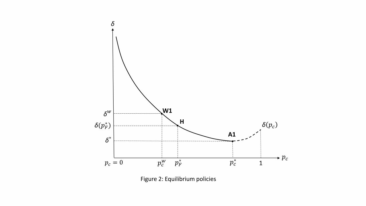
δ

δ 𝑝𝑝𝑐𝑐

1𝑝𝑝𝑐𝑐

Figure 2: Equilibrium policies

A1

𝑝𝑝𝑐𝑐∗𝑝𝑝𝑐𝑐 = 0

..

H

𝑝𝑝𝐹𝐹∗𝑝𝑝𝑐𝑐𝑤𝑤

W1

δ(𝑝𝑝𝐹𝐹∗)δ𝑤𝑤

.δ∗

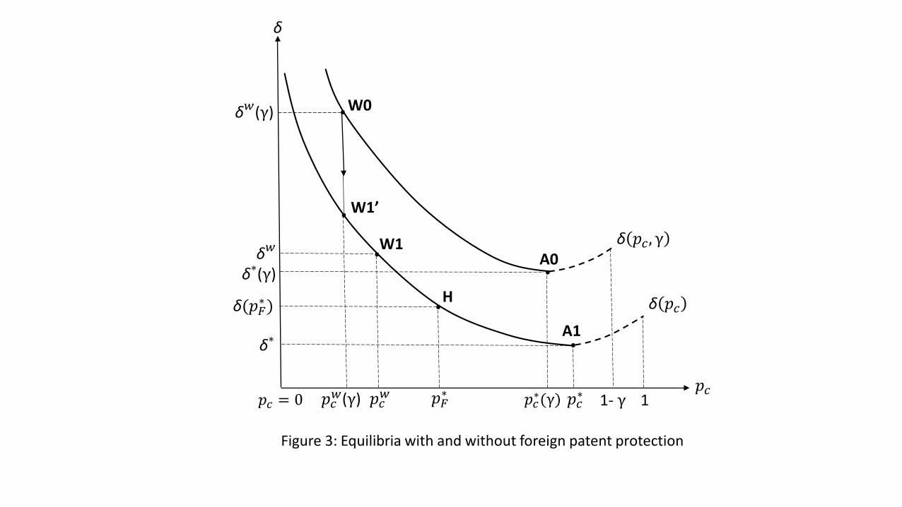
δ

δ 𝑝𝑝𝑐𝑐

1𝑝𝑝𝑐𝑐

Figure 3: Equilibria with and without foreign patent protection

1- γ

W0

A0

A1

𝑝𝑝𝑐𝑐∗𝑝𝑝𝑐𝑐∗(γ)𝑝𝑝𝑐𝑐 = 0

δ 𝑝𝑝𝑐𝑐, γ

..

H

𝑝𝑝𝐹𝐹∗𝑝𝑝𝑐𝑐𝑤𝑤

W1

𝑝𝑝𝑐𝑐𝑤𝑤(γ)

δ(𝑝𝑝𝐹𝐹∗)

δ𝑤𝑤

δ𝑤𝑤(γ) .

.

.δ∗

W1’.

δ∗(γ)

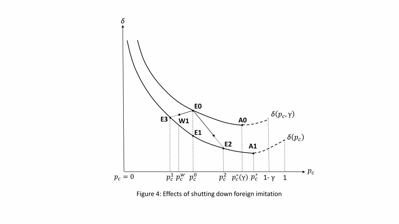
δ

δ 𝑝𝑝𝑐𝑐

1𝑝𝑝𝑐𝑐0𝑝𝑝𝑐𝑐

Figure 4: Effects of shutting down foreign imitation

1- γ

E0

E1

𝑝𝑝𝑐𝑐2

E3

E2

𝑝𝑝𝑐𝑐1

A0

A1

𝑝𝑝𝑐𝑐∗𝑝𝑝𝑐𝑐∗(γ)𝑝𝑝𝑐𝑐 = 0

δ 𝑝𝑝𝑐𝑐, γ...

. .

W1

.

𝑝𝑝𝑐𝑐𝑤𝑤