extending the data mining software packages sas enterprise miner
TRANSCRIPT

Extending the Data Mining Software Packages SAS Enterprise Miner and SPSS
Clementine to Handle Fuzzy Cluster Membership: Implementation with Examples
Donald K. Wedding
A Thesis
Submitted in Partial Fulfillment of the
Requirements for the Degree of
Master of Science in Data Mining
Department of Mathematical Sciences
Central Connecticut State University
New Britain, Connecticut
March 2009
Thesis Advisor
Dr. Roger Bilisoly
Department of Mathematical Sciences

2
Extending the Data Mining Software Packages SAS Enterprise Miner and SPSS
Clementine to Handle Fuzzy Cluster Membership: Implementation with Examples
Donald K. Wedding
An Abstract of a Thesis
Submitted in Partial Fulfillment of the
Requirements for the Degree of
Master of Science in Data Mining
Department of Mathematical Sciences
Central Connecticut State University
New Britain, Connecticut
March 2009
Thesis Advisor
Dr. Roger Bilisoly
Department of Mathematical Sciences
Key Words: Fuzzy Cluster, Fuzzy Cluster Approximation, Fuzzy Membership, Hard
Cluster, SAS Enterprise Miner, SPSS Clementine

3
DEDICATION
This thesis is dedicated to my loving wife, Kathryn and to my wonderful children
Donald, Emily, Katelyn, and our newest son David who was born on February 19 of this
year. Every day with you brings happiness to my life. Your encouragement, love, and
support have given me the strength and the enthusiasm to complete this Master’s degree.

4
ACKNOWLEDGEMENTS
I would like to thank Professors Roger Bilisoly, Dan Larose, and Zdravko Markov, for
agreeing to be on my thesis committee. I am especially grateful to Professor Bilisoly for
acting as my thesis advisor. His efforts were invaluable. I also would like to thank these
same professors along with Professor Dan Miller for the outstanding instruction that I
received in my Masters Degree coursework. I also thank Professor Larose for his
pioneering work in developing this program. He has profoundly influenced my career as
a data miner.
I thank all of my fellow students in the data mining program especially Kathleen Alber
and Judy Spomer (Guinea Pigs #2 and #3). I have learned a great deal from all of you,
and I have made many new friends.
I thank my parents, Donald Sr. and Mary Ellen, who taught me to value education and
learning. I also thank my siblings, Carol, Vicki, and Daniel. You are always there for me
whenever I need you.
I also thank the Lord for leading me to a profession that I love and for all of the other
blessings that are in my life.
5
TABLE OF CONTENTS
DEDICATION................................................................................................................... 3
ACKNOWLEDGEMENTS ............................................................................................. 4
TABLE OF CONTENTS ................................................................................................. 5
ABSTRACT ....................................................................................................................... 7
INTRODUCTION............................................................................................................. 9
Overview of Data Mining: .................................................................................. 10
Growth of Data Mining: ..................................................................................... 10
Importance of Transparency: ............................................................................ 11
Hard Clustering: ................................................................................................. 12
Extending Hard Clusters With Fuzzy Membership: ....................................... 14
Purpose of this Research: ................................................................................... 16
Research Questions:............................................................................................ 17
Relationship of Study to Pertinent Prior Research : ....................................... 17
Research in Fuzzy Clusters: ................................................................... 18
Commercially Available Data Mining Software: ................................. 19
Statement of Need: .............................................................................................. 20
Investigative Procedure to be Followed: ........................................................... 21
Limitations of this Research: ............................................................................. 22
RELATED RESEARCH ................................................................................................ 23
K-Means Algorithm: (Hard Clustering Algorithm) ........................................ 23
Number of Clusters: ............................................................................... 25
Starting Points:........................................................................................ 25
Distance Metrics: .................................................................................... 26
Calculation of New Center Points: ........................................................ 28
Advantages of K-Means: ........................................................................ 30
Disadvantages of K-Means: ................................................................... 31
K-Means Example: ................................................................................. 32

6
Kohonen/SOM Algorithm: (Hard Clustering Algorithm) .............................. 34
Kohonen Network Example: .................................................................. 37
Fuzzy C-Means: (Fuzzy Clustering Algorithm) ............................................... 41
Fuzzy Logic: ............................................................................................ 41
Fuzzy C Means Algorithm: .................................................................... 43
Fuzzy Membership: ................................................................................ 44
Example Of Computing Fuzzy Membership: ...................................... 49
METHODS ...................................................................................................................... 56
Approximating Fuzzy Clusters Using Hard Cluster Techniques ................... 56
Extending SPSS Clementine to Include Fuzzy Membership .......................... 57
SPSS Fuzzy Clementine Fuzzy Membership Work Stream: .............. 58
Example of SPSS Clementine Model: ................................................... 82
Discussion of SPSS Clementine Model: ................................................ 87
Extending SAS Enterprise Miner to Include Fuzzy Membership.................. 88
Example 1 of SAS Enterprise Miner Model: ........................................ 96
Discussion of SAS Enterprise Miner Model: ...................................... 105
Comparison of the Two Approaches ............................................................... 106
Accuracy Improvement of Using Fuzzy Clusters Instead of Hard Clusters 108
CONCLUSION ............................................................................................................. 115
BIBLIOGRAPHY ......................................................................................................... 119
BIOGRAPHICAL STATEMENT ............................................................................... 125

7
ABSTRACT
Clustering is the process of placing data records into homogenous groups. Members of
each group are similar to one another and highly different from members outside the
group. The clusters are used for predictive analysis (what will happen), for explaining
results (why it will happen), and for profiling and understanding data.
Hard clustering and fuzzy clustering are both commonly used by data miners. In hard
clustering, membership is absolute. A record is completely in a cluster or it is completely
out of a cluster so that membership is mutually exclusive. In fuzzy clustering, a record is
permitted to have partial membership so that it is allowed to be in more in one cluster.
For example, a record might be 60% in cluster 1 and 40% in cluster 2. There are
advantages and disadvantages to both hard and fuzzy clustering, and both techniques are
used in research depending upon the data, the type of analysis, and the purpose of the
analysis.
Although both types of clustering are used in research, only hard clustering is provided
by the two most popular commercially available data mining development tools: SAS
Enterprise Miner and SPSS Clementine (note that the graduate student preparing this
research is an employee of the SAS Institute). Thus, if a researcher needs to use fuzzy
clustering, he or she will be unable to use these tools.

8
This research presents a method of approximating fuzzy clusters in both SAS Enterprise
Miner and SPSS Clementine by extending their hard clustering tools to incorporate fuzzy
membership values. Although these fuzzy memberships of hard clusters are only
approximations of fuzzy clusters, it is shown that they can improve accuracy over hard
clustering in some situations. Consequently, they should be added to the list of standard
techniques employed by data miners.

9
INTRODUCTION
Data mining studies data by employing techniques from many different disciplines. It is a
field that has seen significant growth in the past decade, and this growth is projected to
increase for the foreseeable future. Organizations use data mining techniques on their
data because it can be used to both predict and explain events. For example, data mining
can be used to predict which customers will attrite and then explain why the customers
are leaving. It can explain which advertising campaigns will be successful and why the
targeted customers will respond. It can be used to predict which voters will support a
candidate and what issues are important to them.
One of the most common techniques employed in data mining is cluster analysis, which
is the process of grouping similar data points together into homogenous groups. After
these clusters are identified, they are analyzed so that the features that make them
different from other groups can be uncovered. These differences can be used to explain
why one cluster behaves differently from another.
Virtually every major data mining reference and commercially available data mining
program includes clustering. However, these major references and programs tend to deal
strictly with hard clusters (where membership is limited to one and only one cluster) and
fail to mention or incorporate fuzzy clusters (where membership in a group is partial and
can be spread out over many clusters). The purpose of this research is to discuss fuzzy

10
clustering and to describe how to incorporate it into a data mining analysis, even if the
software being used does not offer fuzzy clustering.
Overview of Data Mining:
Data mining finds useful patterns and extracts actionable information from what are
called “dirty” data sets. These are typically large, have highly correlated variables, and
can contain many missing and incorrect values. Data mining uses techniques from
statistics, artificial intelligence, expert systems, and data visualization and focuses on
practical results. This is similar to a civil engineer who applies physics, chemistry,
material science, meteorology, economics, and law so that a bridge can be built.
Similarly, a business wants practical answers to questions such as the following:
Which customers are likely to attrite?
Who should we loan money to and what interest rate should we charge?
Where should we build a new gas station?
Who is likely to crash their car in the next six months?
Growth of Data Mining:
If a business is able to tap into the vast amounts of data that it collects, it may identify a
better way of operating; and it can gain an advantage over its competition. Clearly data
mining has major financial implications to an organization, which explains why it has

11
gained so much interest within the past 10 years. For example, in 2000, MIT Technology
Review listed data mining as one of the ten emerging technologies that will change the
world (Fried, December 28, 2000). In another report it was predicted that “data mining
will be one of the most revolutionary developments of the next decade” (Konrad,
February 9, 2001).
There are currently no signs that needs and demands for data mining will abate. For
example, in a report published by IBM it was forecasted that the “world’s information
base will be doubling in size every 11 hours.” (IBM, 2006 p.2). Even if that estimate
ultimately proves to be overly aggressive, the fact still remains that the doubling time is
speeding up. With the increase of data, there will certainly be a greater need for data
mining to analyze this data.
Importance of Transparency:
A “black box” that can give a prediction of which customer, for example, will attrite is
useful, but only up to a point. A business would like to know not only who will leave, but
why they will leave. Without this understanding, the information is of limited value
because then the business would not know how to keep the customer from attriting. This
is why understanding the results are so important. Larose referred to this understanding as
transparency. “Data mining models should be as transparent as possible. That is, the
results of the data mining models should describe clear patterns that are amenable to
intuitive interpretation and explanation” (Larose 2005 p.11).

12
Hard Clustering:
Clustering is the process of placing data into homogenous or similar groups. Each cluster
or group is analyzed to determine how it is different from other groups.
For example, a business might cluster customers based on their demographic information
(age, gender, marital status, children, and income). The algorithms might yield several
distinct groups of data such as a cluster of affluent people who are married with teen age
children. The business might then look more closely at this group and find that they are
more profitable than other segments, yet they have a much higher attrition rate. Further
investigation might yield that this group is most concerned with good service and is not
price sensitive. Consequently, a business might devise a special program for these
customers to ensure that they receive the best service possible in order to reduce their
attrition. In addition to customer treatments, the cluster membership can be used as inputs
into predictive models as a surrogate for complex data interactions. As opposed to having
an interaction of the five variables used for clustering, a single Boolean (“True” or
“False”) flag indicating membership could be incorporated into the predictive model.
In fact, clustering is such a prevalent technique in data mining that virtually every major
text on the subject contains information on it (Berry and Linoff, 2000; Berry and Linoff
2004; Hand, Mannila, and Padhraic, 2001; Larose, 2005; Larose, 2006; Parr Rud, 2001).
Clustering techniques are also included in nearly every major commercially available

13
data mining software platform including the two industry leaders: SAS Enterprise Miner
(note that the graduate student preparing this research is an employee of the SAS
Institute) and SPSS Clementine (Gartner, July 1, 2008).
There are many different methodologies to clustering described in the literature, but the
most widely used techniques K-Means clustering (MacQueen, 1967; Hartigan, 1975;
Hartigan and Wong, 1979; Lloyd, 1982) and Self Organizing Maps (SOM) which are
also referred to as Kohonen networks (Kohonen, 1988). Because of their widespread use,
they are covered in the data mining texts and the techniques implemented in the major
commercial data mining software.
The K-Means and the Kohonen clustering techniques incorporate significantly different
algorithms, yet they share one characteristic: they are hard clustering techniques. A hard
clustering algorithm only permits membership in one group. Membership in a cluster is
mutually exclusive to all other clusters. For example, assume that a collection of data is
clustered into three groups that are labeled A, B, and C. If a data point is placed into one
of the three groups then it will be in that group and only that group. A data point in group
“A” means that the data point is not in either group “B” or group “C”. Similarly, a data
point in group “B” or “C” would also be mutually exclusive to the other clusters.
This concept of mutual exclusion can be convenient in clustering for several reasons.
First, it makes the clustering process quick. Secondly, it makes analysis and interpretation

14
simple. Finally, hard cluster membership can be treated as a Boolean flag that can be
used in other data mining techniques that require discrete variables instead of continuous.
Extending Hard Clusters With Fuzzy Membership:
Fuzzy clustering relaxes the requirement that cluster membership be mutually exclusive.
In other words, a data point may have membership in two or more clusters with the
cluster membership summing to one.
Fuzzy clustering is an extension of the concept of fuzzy logic which was pioneered by
Lotfi Zadeh in his seminal work introduced in 1965 (Zadeh, 1965). The idea of fuzzy
clustering is to quantify ambiguity in language. For example, a person might be defined
as “tall” if they are 6 feet tall. In Boolean algebra, if a person were 6 feet tall then the
logical variable, TALL, would be set to 1 (for true). A person who was 4 feet would have
the logical variable TALL set to 0 (for not true). Now consider a person who is 5 feet 11.9
inches. This person does not meet the strict definition of tall. In the Boolean world, the
value for TALL would be set to 0. This person would be treated the same as a person who
was 4 feet tall. This is counterintuitive to how humans view the world. In fuzzy logic, the
person who was 5 feet 11.9 inches could have a partial membership in the TALL variable.
So this person might have a TALL value of, say, 0.95. As the person’s height is reduced
then their membership in the TALL variable is also reduced until at some point the
membership reaches 0.

15
Fuzzy clustering is an extension of this concept. It permits a data point to have partial
membership in more than one cluster. Fuzzy clustering is a major field of study and there
are many different algorithms for partial membership classification, but one of the most
widely used and cited is the Fuzzy C-Means algorithm developed by James Bezdek
(Bezdek, 1981). This algorithm is simple, fast, and gives practical results for many
diverse real world data sets. In order to appreciate how widely Bezdek’s work is utilized,
the title of his work “Pattern Recognition with Fuzzy Objective Function Algorithms”
and the name Bezdek were entered into Google (http://www.google.com/) on September
8, 2008. The results returned indicate that it was referenced on “about 30,500” web sites
and was cited 4,884 times. The Google search was run second time on February 12, 2009
but this search was restricted only to the Citeseer domain by using the option:
site:citeseer.ist.psu.edu. This search retrieved 396 references to Bezdek’s work.
Despite the wide usage of fuzzy clustering, it is not yet widely employed in mainstream
commercial data mining. As evidence, refer to the leading texts on the subject and it can
be seen that it is rarely mentioned. Furthermore, the two leading data mining software
platforms SAS Enterprise Miner and SPSS Clementine (Gartner, July 1, 2008) do not
include any fuzzy clustering functionality.

16
Purpose of this Research:
In this thesis, three tasks will be completed:
1. Programs in Enterprise Miner and SPSS Clementine will be written to calculate
fuzzy cluster memberships.
2. A technique will be given to implement fuzzy clustering in both K-Means and
Kohonen clusters for both of these software platforms.
3. A simple model will be built to demonstrate how fuzzy clustering can improve
accuracy of some models. Advantages and disadvantages to fuzzy clustering will
be discussed.
There are two goals to this research. First it is anticipated that persons in the field of data
mining, whether novice or skilled practitioner, will be convinced of the effectiveness of
fuzzy clustering.
The second purpose of this research is for this document to serve as a blueprint on how to
utilize fuzzy clustering given software that does not implement it. It is conceivable that
fuzzy clustering may be added to the curriculum in the Central Connecticut State
University MS Data Mining program by including it in one of the introductory data
mining classes.

17
Research Questions:
The research in this thesis will address four questions:
1. How can Fuzzy Clustering be implemented using the existing hard K-Means
Clustering and/or hard Kohonen clustering as implemented in SPSS Clementine?
2. How can Fuzzy Clustering be implemented using the existing hard K-Means
Clustering and/or hard Kohonen clustering as implemented in SAS Enterprise
Miner?
3. Can Fuzzy Clustering in some cases be shown to give improved results over hard
clustering?
4. What advantages and disadvantages were encountered during this research of
which practitioners in data mining should be aware?
Relationship of Study to Pertinent Prior Research :
The pertinent prior research focuses on two areas. First, there is research related to fuzzy
clustering. This section will demonstrate that fuzzy clustering techniques are widely used
and that they are being employed in many different areas. The second area of pertinent

18
research will focus on the commercially available data mining software. This section will
show that the two most significant commercial software platforms in data mining are
SAS Enterprise Miner and SPSS Clementine. These are judged based upon their market
share and how their functionality is rated by an independent party.
Research in Fuzzy Clusters:
Fuzzy Clustering is widely used in many fields of research. For example, Bezdek’s
seminal paper on Fuzzy Clustering returned over 30,500 web pages on Googletm
and was
cited nearly 5000 times. Additionally, when the terms “fuzzy cluster” and “data mining”
were used as search terms, there were 4350 web pages returned by Googletm
(http://www.google.com/) on September 11, 2008. Fuzzy clustering is employed in a
wide number of disciplines, including the following:
Climate and weather analysis (Liu and George, 2005)
Analysis of network traffic (Lampinen, Koivisto, and Honkanen, 2002),
Soil analysis (Goktepe, Altun, and Sezer 2005)
Database Marketing (Russell and Lodwick, 1999)
Medical Image Classification (Wang, Zhou, and Geng, 2005)

19
The idea of fuzzy membership has also been extended to include Self Organizing Maps
(Bezdek, Tsao, Pal 1992). The premise behind this approach is to use the fuzzy
membership functions described by Bezdek (Bezdek, 1981) with Kohonen’s training
algorithm (Kohonen, 1988). This approach to fuzzy clustering is also widely used. Again
employing the Googletm
search technique, it is observed that a search that includes "Fuzzy
Kohonen Clustering Networks" OR "fuzzy som" OR "fuzzy kohonen"
(http://www.google.com/) on September 13, 2008 returned 3850 references. As with
fuzzy clustering, the fuzzy Kohonen technique is found in a variety of areas including:
Drug discovery (Shah and Salim 2006).
Image Segmentation (Wang, Lansun, an Zhongxu 2000)
Tumor Classification (Granzow, Berrar, Dubitzky, Schuster, Azuaje, and Eils
2001)
In summary, fuzzy clusters are used in both K-Means and Kohonen clustering. It is
applied to numerous research areas in many different fields. It has not, however, been
incorporated into mainstream commercial applications of data mining.
Commercially Available Data Mining Software:
The two most prominent developers of data mining software are SAS and SPSS. SAS is
the largest vendor in this area according to Gartner and by empirical observation SPSS is
most likely the second largest. Both of these companies offer specialized tools designed

20
for data mining: SAS offers Enterprise Miner (EM) version 5.3 and SPSS offers
Clementine version 12.0.
Both of these products are widely used and they are both considered to be the best
commercially available data mining software. In fact, as of June 2008, SAS Enterprise
Miner and SPSS Clementine were the only two data mining products listed as Leader in
the Gartner Magic Quadrants on Gartner.com. Gartner defines this term as:
Leaders are vendors that can meet the majority of requirements for most
organizations. Not only are they suitable for most enterprises to consider,
but they also have a significant effect on the market’s direction and
growth. (Gartner 2008).
Therefore, both of these two products are clearly in wide use and they are both judged as
leaders in the commercial data mining space.
Statement of Need:
SAS Enterprise Miner and SPSS Clementine are the two leading commercially available
software packages in data mining, yet neither one offers fuzzy clustering despite its
widespread use. Users of both software packages would benefit from a methodology to
incorporate fuzzy memberships using these products. For example Bruce Kolodziej, a
former CCSU Data Mining student and current Systems Engineer of SPSS specializing in

21
Clementine, stated that there is a demand for fuzzy clustering. As an example, he stated
that one sales prospect wanted to determine if Clementine could indicate the second
choice and third choice for cluster membership. The Systems Engineer devised a
technique to calculate the second and third closest distances to the cluster centers
(Kolodziej, 2008). Calculating the distances to the nearest other cluster centers is the first
step in fuzzy clustering. Calculating partial membership of the clusters would be a logical
next step in this case.
Therefore, this research addresses the need to implement fuzzy clustering using K-Means
and/or Kohonen hard clustering. After the fuzzy clustering has been developed, a model
will be built to determine if fuzzy clusters improve the accuracy of a predictive model
over hard clustering.
Investigative Procedure to be Followed:
1. Generate flow diagrams for SPSS Clementine which can be used in conjunction
with both K-Means and Kohonen models in order to calculate fuzzy membership.
In this case, a “flow diagram” will be either executable software or executable
icons that will reside inside of either tool. In either case, these will be used to
actually generate real fuzzy values. These will not merely be theoretical concepts,
but instead will be practical and usable software.

22
2. Generate flow diagrams and/or SAS Code and/or SAS Macro Code for SAS
Enterprise Miner which can be used in conjunction with K-Means and/or
Kohonen models in order to calculate fuzzy membership.
3. Some trivial clusters and data will be entered into both SAS Enterprise Miner and
SPSS Clementine. The cluster memberships will be compared with manual
calculations. If the software gives the same answers as the hand calculations, this
will suggest that the approach is correct.
4. A simple predictive model will be built that will employ both hard and fuzzy
clustering. The clusters will be used to predict some outcome. It will be shown
that in some cases the fuzzy clusters can achieve better results than hard clusters.
This will suggest that fuzzy clusters are a viable technique in data mining.
Limitations of this Research:
Because both SAS Enterprise Miner and SPSS Clementine use only hard clustering
techniques, the cluster centers used for fuzzy membership will be different than if they
had been calculated using fuzzy techniques. In other words, the fuzzy cluster membership
will be based on hard clusters. Therefore, this will be an approximation of true fuzzy
cluster centers.

23
Further limitations will be based on the software being used. For example, there may be
limitations on transformations of data or in distance metrics that are implemented.
Therefore, data mining techniques employed will be subject to the limitations of the
software.
RELATED RESEARCH
This chapter describes both the hard and fuzzy clustering techniques that will be utilized
in this research. The two hard clustering techniques described are K-Means algorithm and
the Kohonen Neural Network (also called the Self Organizing Map (SOM)). The fuzzy
clustering technique that will be used is the Fuzzy C Means, which is a generalized case
of the K-Means algorithm.
K-Means Algorithm: (Hard Clustering Algorithm)
The K-Means algorithm is a hard clustering methodology that places data in k distinct
groups. It is one of the most widely used clustering algorithms because it is a simple
algorithm to implement, quick to converge, and tends to give good results. The K-Means
algorithm was initially described by Lloyd in 1957 at Bell Telephone Laboratories, but he
did not formally publish until 1982 (Lloyd, 1982). Most authors reference MacQueen or
Hartigan who described the algorithm in 1967 and 1975 respectively (MacQueen, 1967;
Hartigan, 1975).

24
The general form for the K-Means algorithm is provided below.
1. For a data set consisting of N data points, select the desired number of clusters, k,
where k < N.
2. Generate a starting center point for each of the k clusters.
3. Calculate the distance from each of the N points to each of the k clusters.
4. Assign each of the N points to the cluster that is closest to it
5. Find the new center point for each of the k clusters.
6. Repeat steps 3, 4, and 5 until there are no changes in the cluster membership.
This algorithm is flexible enough that programmers and analysts frequently use it as a
guideline, but they will modify it to suit their application and the data that is available.
Some common modifications include:
Determination of the number of clusters
Generating the starting center points for each cluster
Distance metrics from a point to a given cluster center
Calculation of new center points
Each of the variations to the K-Means clustering algorithm are presented in greater detail
in the following sections.

25
Number of Clusters:
The results of the K-Means algorithm depend upon the number of clusters (the k value).
If k is too small, then there will be too many data points in each cluster which could
obscure useful information. This would be similar to under-fitting a predictive model. If
there are too many clusters, then the algorithm will likely split on insignificant variables
or noise which would be similar to over-fitting a predictive model. There is no way to
determine the best number of clusters, but there are some techniques to estimate a good
number of clusters. Common techniques for estimating the optimal number of clusters
range from trial and error to sophisticated algorithms (Sarle, 1983; Milligan G.W., 1996;
Zhang et al., 1996).
Starting Points:
The starting center points of the k clusters will impact the final results. This is because
the K-Means algorithm can get stuck at local optimum solution instead of finding the
global optimal solution. Therefore, if the algorithm is run twice on the same data but with
different starting points then the final clusters can be significantly different from one
another. As with the number of clusters, there is no best way to generate the starting
points, but there are some commonly used techniques. These are described below.
Use a Random Number Generator to produce the centers
Randomly select k points from the data and use them as starting points
Select the first k points in the data set
Select the k points in the data set that are furthest from one another
26
Distance Metrics:
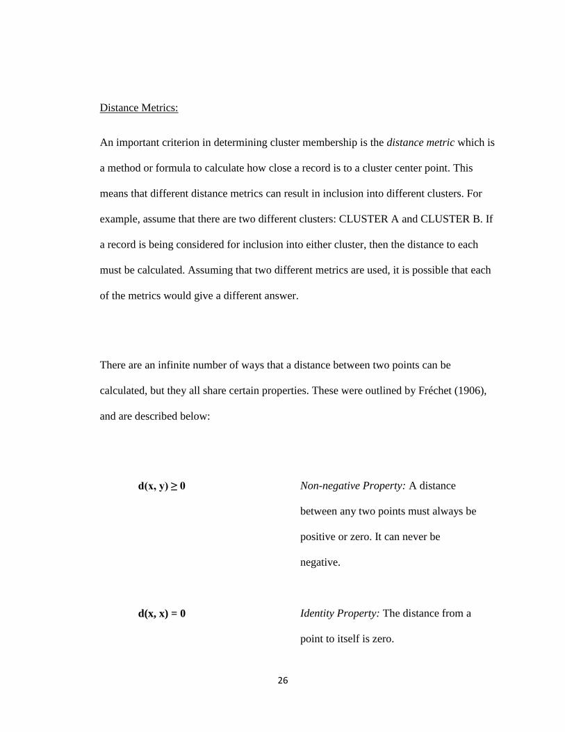
An important criterion in determining cluster membership is the distance metric which is
a method or formula to calculate how close a record is to a cluster center point. This
means that different distance metrics can result in inclusion into different clusters. For
example, assume that there are two different clusters: CLUSTER A and CLUSTER B. If
a record is being considered for inclusion into either cluster, then the distance to each
must be calculated. Assuming that two different metrics are used, it is possible that each
of the metrics would give a different answer.
There are an infinite number of ways that a distance between two points can be
calculated, but they all share certain properties. These were outlined by Fréchet (1906),
and are described below:
d(x, y) ≥ 0 Non-negative Property: A distance
between any two points must always be
positive or zero. It can never be
negative.
d(x, x) = 0 Identity Property: The distance from a
point to itself is zero.

27
d(x, y) = d(y, x) Symmetric Property: The distance of
going from point x to point y is the
same as going from point y to point x.
This implies that there will not be any
“one way streets” in a distance metric.
d(x, y) ≤ d(x, z) + d(z, y) Triangle Property: This is another way
of saying that the shortest distance
between two points is a straight line. It
is impossible shorten the distance from
x to y to z.
A common approach to calculating distance is the Power Norm Distance given in
Equation 1. This metric takes the difference of each element of the vector and raises it to
the power of P, then sums these values and takes the root of R. Typically P and R are set
to the same value which is the LP Norm or the Minkowski distance of order P, but there
is no requirement for P and R to be equal.
𝒅 = 𝒙𝒊 − 𝒚𝒊 𝑷
𝑵
𝒊=𝟏
𝟏𝑹
Equation 1
28
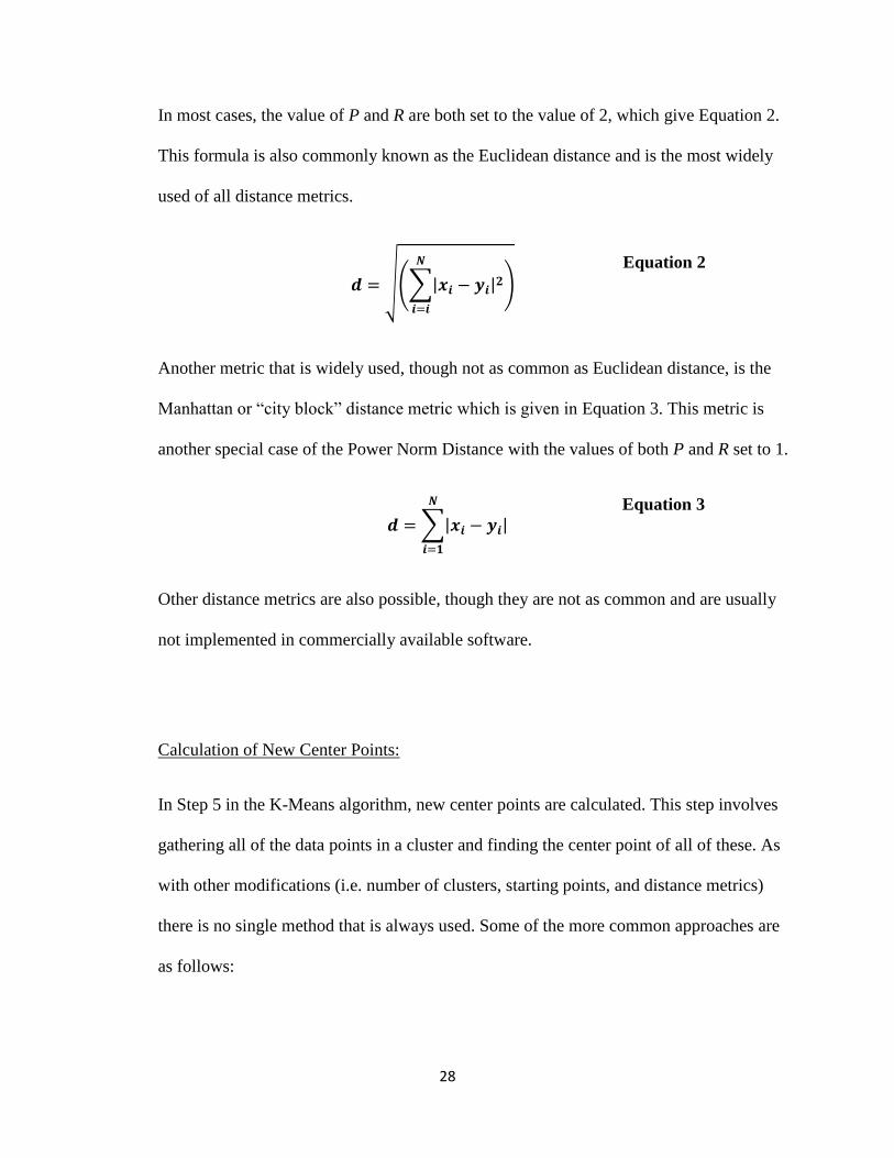
In most cases, the value of P and R are both set to the value of 2, which give Equation 2.
This formula is also commonly known as the Euclidean distance and is the most widely
used of all distance metrics.
𝒅 = 𝒙𝒊 − 𝒚𝒊 𝟐𝑵
𝒊=𝒊
Equation 2
Another metric that is widely used, though not as common as Euclidean distance, is the
Manhattan or “city block” distance metric which is given in Equation 3. This metric is
another special case of the Power Norm Distance with the values of both P and R set to 1.
𝒅 = 𝒙𝒊 − 𝒚𝒊
𝑵
𝒊=𝟏
Equation 3
Other distance metrics are also possible, though they are not as common and are usually
not implemented in commercially available software.
Calculation of New Center Points:
In Step 5 in the K-Means algorithm, new center points are calculated. This step involves
gathering all of the data points in a cluster and finding the center point of all of these. As
with other modifications (i.e. number of clusters, starting points, and distance metrics)
there is no single method that is always used. Some of the more common approaches are
as follows:

29
Mean Value: This is the most widely used method of finding the center point. In
this method, all of the values for each variable are added up and divided by the
number of points. This approach is simple to compute and usually gives good
results but is sensitive to outliers.
Median Value: This is another widely used approach but not as prevalent as the
Mean. It is not as sensitive to outliers, but has the problem of treating all values
with equal weight. This might have the effect of understating or overstating a
center point. Also, this approach requires sorting so it can be time consuming for
large data sets.
Medoid Value: This approach requires the center to be an actual point within the
cluster. So if there were 10 points in the cluster, then one of the 10 points would
be the center point. The point chosen would have to smallest total distance to all
of the other points. This approach is not sensitive to outliers, but can be time
intensive to compute.
Hybrid Value: There is no reason that the center point should be computed the
same way for all variables. The center point could just as easily be a hybrid
approach. For example, if the 10 data points in a cluster each have three variables,
X, Y, and Z then the center point might be computed as: Mean of X, Median of Y,
and Medoid of Z. The problem with this approach is that it is difficult to compute
and it is unlikely that any commercially available software will implement it.

30
Also, there is no evidence that this approach may be any better or worse than any
other technique.
Advantages of K-Means:
As previously stated, the K-Means algorithm is a simple algorithm that can arrive at a
solution quickly and can give good results. These two qualities make it is one of the most
widely used clustering methods.
Simple to Implement: The algorithm has only a few steps that consist of finding
distances and moving a data point to a cluster. This simplicity allows analysts and
programmers considerable flexibility during implementation.
Quick to Converge: In most cases, the K-Means algorithm converges to a solution
quickly. Duda et. al claim that “In practice the number of iterations is generally
much less than the number of points” (Duda, Hart, and Stork, 2000). However, it
has been shown by Arthur and Vassilvitskii (Arthur and Vassilvitskii 2006) that it
was possible using adversarial cluster centers to slow convergence down to at
least 2𝛺( 𝑛) iterations where 𝛺 𝑛 is Landau notation (Landau, 1909) for some
function of n½
. Arthur and Vassilvitskii were unable to explain the difference
between this theoretical value and observed performance. The author of this text
proposes that perhaps it may have something to do with the fact that most analysts
do not go out of their way to choose adversarial starting points.
Good Results: The K-Means algorithm can yield intuitive, predictive, and
actionable results. This can be empirically demonstrated by the fact that the

31
algorithm is widely used and is implemented in most commercially available
software that offers clustering.
Disadvantages of K-Means:
The K-Means algorithm also has some disadvantages associated with it. These
disadvantages are discussed below. Fortunately, when the K-Means algorithm is
implemented in a commercial product, the software designers usually give analysts
options to mitigate these disadvantages. These are also discussed below.
No Way to Determine Optimal Number of Clusters: A disadvantage to the K-
Means algorithm is that it requires the user to specify k, the number of clusters,
but in most cases the analyst does not know the appropriate number of clusters.
Thus, the analyst must rely on exploring the data and then taking an educated
guess based on experience with the data and the domain. In the opinion of the
author, this can produce satisfactory results.
Sensitivity To Starting Values: The starting center points have great influence on
the final clusters. This is because the K-Means algorithm can converge to local
optimal points instead of a global or “best” solution. With commercially available
software, the analyst usually is given different options for selecting the starting
points. So an analyst will have flexibility to try different starting points to increase
the probability that the global optimum (or at least a very good local optimum)
will be found.

32
Winner Take All: Finally, the K-Means algorithm is a hard clustering algorithm
which is also referred to as “winner take all”. In other words, if a point lies
between CLUSTER1 and CLUSTER2, and is just barely closer to CLUSTER1,
then it will be completely in CLUSTER1 and not at all in CLUSTER2 even
though it could be argued that it was almost as close to that cluster. Furthermore,
this point that just barely lies within CLUSTER1 will be treated exactly the same
as a data point that lies directly on the cluster’s center point. In some cases, this
will not cause issues, but there may be cases where it is desirable to allow a point
to have memberships in more than one cluster. As of the writing of this document
neither SAS Enterprise Miner nor SPSS Clementine incorporates fuzzy cluster
membership.
K-Means Example:
The following example will go through a single iteration of the hard clustering algorithm.
The data points were taken from Höppner, et. al, (Höppner, Klawonn, Kruse, and
Runkler, 1999) who used the points for a fuzzy clustering example. In this example, there
are two clusters and the Euclidean distance metric is used (see Equation 2). The starting
two cluster center points are arbitrarily set to the values of:
C1 : (0.8, 0.2)
C2: (0.2, 0.8)

33
Applying the distance formula of Equation 2 to the six data points given in Table 1 result
in the distance values presented in the table. Each data point is assigned a cluster
membership based upon which of the cluster centers is closest to the point.
Data Point Distance to C1 Distance to C2 Membership
1
7,6
7 0.929 0.081 C2
2
7,3
7 0.563 0.381 C2
3
7,5
7 0.634 0.244 C2
4
7,2
7 0.244 0.634 C1
5
7,4
7 0.381 0.563 C1
6
7,1
7 0.081 0.929 C1
Table 1 Hard Cluster Example Problem Data
With the cluster memberships assigned, new center points are calculated using the mean
average of all of the points within the cluster. Using the values in Table 1, the new center
points are calculated as:

34
C1 = {(4/7, 2/7) + (5/7, 4/7) + (6/7, 1/7)} / 3
= (0.714, 0.333)
C2 = {(1/7, 6/7) + (2/7, 3/7) + (3/7, 5/7)} / 3
= (0.286, 0.667)
The process described above will continue until there are no changes in the cluster
membership assignments. This would indicate that the algorithm has converged. In the
above example, further iterations will yield the same result, so therefore this example has
converged.
Kohonen/SOM Algorithm: (Hard Clustering Algorithm)
Kohonen networks were introduced in 1982 (Kohonen, 1982) as a tool for sound and
image analysis. They are a type of self organizing map (SOM) because they map
complex, high dimensional data, to discrete, low dimensional groups or clusters. Even
though it was designed for high dimensional data, it is often applied to low dimensional
clustering that is found in data mining applications. It is a powerful technique for
clustering, and like K-Means it is often implemented in commercially available data
mining software such as SAS Enterprise Miner and SPSS Clementine.
There are many similarities between the K-Means algorithm and the Kohonen algorithm.
The most significant similarities are the use of a distance metric and the methods for

35
generating of starting points. Both of these concepts were already described in the
previous section. The differences between the two algorithms are described below.
Kohonen clusters have two important differences to K-Means clusters. First, the Kohonen
networks have a competitive learning algorithm where each cluster competes for data
records. If a cluster is able to capture a record, then it is rewarded by adjusting its
parameters so that it will have an easier time capturing similar records in the future. Also,
the clusters that are close to the winning cluster are also rewarded so that they will also
have an easier time capturing similar data in the future. A consequence of this learning
algorithm leads to the second important difference with K-Means which is that adjacent
clusters in the Kohonen clusters are similar to one another while clusters that are far away
will be significantly different.
The general form for the Kohonen algorithm is provided below, and can be found in
greater detail in Larose (Larose, 2005) and in Fausett (Fausett, 1994).
1. For a data set consisting of N data points, select the desired dimensions of the Kohonen
(usually a two dimensional architecture with P rows and Q columns where P*Q < N).
2. Generate a starting center point for each of the clusters.
3. Competition: Select a record from the N data points and calculate the distance from that
data point to each of the cluster centers. Determine the closest cluster.
4. Adaption: Reward the winning cluster by adjusting its center point so that it moves closer
to the record.

36
5. Cooperation: Determine all of the clusters that are adjacent to the winning cluster and
move them closer to the record.
6. Repeat to steps 3, 4, and 5 until all of the records have been classified.
7. Reclassify all of the data until there are no changes or until some other convergence
criteria has been met.
In steps 4 and 5 of the algorithm, the center points are adjusted using Equation 4.
𝒄𝒊,𝒋(𝒏𝒆𝒘) = 𝒄𝒊,𝒋(𝒐𝒍𝒅) + 𝜼(𝒙𝒏,𝒊 − 𝒄𝒊,𝒋(𝒐𝒍𝒅)) Equation 4
In Equation 4, the c value is the center of the cluster that is being adjusted. The value i
represents the dimension of the center point, and j is the index of the cluster. The value x
represents the n-th record that is being classified. The value of η is a learning constant
which affects the rate of updating the center points. Its value is in the range of 0 < η < 1.
As with the K-Means algorithm, there is flexibility with the implementation of the
Kohonen network algorithm. Referring to the section on K-Means, the Kohonen
networks can be customized with respect to the following areas listed below. Each was
discussed in the previous section.
Determination of the number of clusters
Generating the starting center points for each cluster
Distance metrics from a point to a given cluster center
Calculation of new center points

37
In addition to the four variations listed above, it is also possible to modify the adjustment
formula given in Equation 4. Two typical modifications involve the learning constant, η.
In the first modification, a different η value is used for the winning cluster and a slightly
lower value of η is used for the adjacent clusters. This causes the reward to be greater for
the winner cluster than it would be for the adjacent clusters. A second variation to this
algorithm involves gradually decaying the η value after each of the iterations. The effect
of this decay is to speed up convergence of the algorithm.
Kohonen Network Example:
The following example demonstrates the Kohonen algorithm by stepping through a single
training iteration. This example will also show the differences between the K-Means
algorithm and the Kohonen algorithm. The data used for these calculations is the
Wisconsin Breast Cancer Data Set (Mangasarian, and Wolberg, 1990; Wolberg and
Mangasarian, 1992). This data set has 699 records, each with 11 features. However, for
this example, only two features will be used from the data set, the Bland Chromatin and
Clump Thickness. Both of these features have values that range from 1 to 10 inclusive,
but in both cases the data points were standardized. The values used for standardization
were as follows:
Bland Chromatin
Mean : 3.438
Standard Deviation : 2.438
Clump Thickness
Mean : 4.418
Standard Deviation : 2.816

38
It was arbitrarily decided that the data would be grouped into a 3x3 network and that the
initial cluster centers would be the first 9 data points after the records had been sorted by
the ID number in ascending order.
Each of the starting points have been standardized. The first value in each center point is
the standardized value of the Bland Chromatin feature, and the second value is the Clump
Thickness feature. The starting data points are given in Table 2.
0 1 2
0 (-0.590, 0.207) (1.461, 1.627) (1.051, 1.983)
1 (1.461, 0.562) (0.641, -1.214) (2.281, 0.917)
2 (1.461, 1.272) (-0.180, 1.272) (1.871, 0.207)
Table 2 Starting Points for Kohonen Network Example: First 9 Data Points
Assuming that the Training point (-0.180, -0.148) is entered into the network. The
network will be updated using the Kohonen network. For this exercise, assume that only
vertically and horizontally adjacent and not diagonally adjacent cells in the network will
be updated. Also assume that the learning rate constant, η, is set to 0.1 and the distance
metric is the Euclidean distance (Equation 2).

39
Referring to the Kohonen algorithm, the first step in the algorithm is to calculate the
distance from the training point to each of the cluster centers. These values are given
below.
Distance to Row 0, Column 0 : 0.543
Distance to Row 0, Column 1 : 2.417
Distance to Row 0, Column 2 : 2.461
Distance to Row 1, Column 0 : 1.788
Distance to Row 1, Column 1 : 1.345
Distance to Row 1, Column 2 : 2.681
Distance to Row 2, Column 0 : 2.170
Distance to Row 2, Column 1 : 1.421
Distance to Row 2, Column 2 : 2.081
The smallest distance from the above list is 0.543, therefore the closest cluster to the
training point is Row 0, Column 0. This is the winning cluster and it must be adjusted so
that it will be closer to the input point (-0.180, -0.148). In addition to the winning cluster,
the clusters that are adjacent to the winning cluster are also adjusted. In total, the
following clusters will be adjusted:
Row 0, Column 0 (winning cluster)
Row 0, Column 1 (next to the winning cluster)
Row 1, Column 0 (next to the winning cluster)
The formula for adjusting the centers was given in Equation 4. This equation is applied to
the cluster center for Row 0, Column 0 and the math presented below. The calculations
for Row 0, Column 1 and Row 1, Column 0 are the same, but are not shown.

40
𝒄𝒊,𝒋(𝒏𝒆𝒘) = 𝒄𝒊,𝒋(𝒐𝒍𝒅) + 𝜼(𝒙𝒏,𝒊 − 𝒄𝒊,𝒋(𝒐𝒍𝒅))
= (-0.590, 0.207) + 0.1[(-0.180, -0.148) - (-0.590, 0.207)
= (-0.590, 0.207) + (0.041, -0.036)
= (-0.549, 0.171)
The new cluster centers are shown in Table 3. Referring back to the K-Means example, it
is important to note the differences in the training between the K-Means and the Kohonen
networks. In the K-Means, all of the training points were assigned membership and then
the center points were adjusted. In the Kohonen algorithm, each training point is used one
at a time and the center points are adjusted after each training point is entered.
0 1 2
0 (-0.549, 0.171) (1.297, 1.445) (1.051, 1.983)
1 (1.297, 0.491) (0.641, -1.214) (2.281, 0.917)
2 (1.461, 1.272) (-0.180, 1.272) (1.871, 0.207)
Table 3 New Center Points after training iteration
Another difference is that a training point in the Kohonen network can cause more than
one center point to be adjusted in a training iteration. This gives clusters that are similar
to those around them. Refer to the center points presented in Table 4, which were
determined using SAS Enterprise Miner on the Wisconsin Breast Cancer Data.
0 1 2
0 (1.753, 1.596) (0.130, 1.566) (-0.807, 0.282)
1 (1.745, 0.058) (-0.041, 0.168) (-0.752, -0.354)
2 (-0.051, -0.504) (-0.109, -1.122) (-0.810, -1.128)
Table 4 New Center Points after training is completed.
41
Notice that the trained Kohonen network has center points that follow a pattern. Moving
from left to right and top to bottom, the values for Bland Chromatin and Clump Thickness
get progressively smaller. The further a cell is from another cell on the Kohonen map, the
more different are the two center points. This difference is more pronounced because
only two features were used in this analysis. It may be more difficult to observe a pattern
when more features are used.
Fuzzy C-Means: (Fuzzy Clustering Algorithm)
The previous sections presented the K-Means and the Kohonen clustering algorithms. In
both of these clustering methods, the algorithms produced clusters where membership
was completely restricted to one and only one cluster. These types of clusters are referred
to as hard clusters.
In this section, a different algorithm is presented that allows a record to be a member of
multiple clusters. That is, membership is now a partial membership in any given cluster.
Cluster membership of this type is referred to as fuzzy cluster membership, which is a
logical extension of fuzzy logic which was pioneered by Zadeh (Zadeh, 1965). There are
many different methods of generating fuzzy clusters, but the most widely used was
described by Bezdek (Bezdek, 1981). This is the approached used in this research.
Fuzzy Logic:
Fuzzy logic was originally presented by Zadeh in the 1960’s as an approach to
quantifying concepts that are imprecisely described by human language. The idea behind

42
fuzzy logic is that it expands upon the limitations of Boolean logic where something must
be either true or false. Fuzzy logic allows for something to be partially true and partially
false.
Consider a situation where a person is described as “TALL”. In Boolean logic, that
statement is either accurate (true) or inaccurate (false). For example, there is little doubt
that former NBA basketball player, Kareem Abdul-Jabbar at 7 feet 2 inches tall, would be
considered TALL. Likewise, former NBA player, Spud Webb at 5 feet 6 inches tall,
would not be considered TALL (he was third shortest man to ever play in the NBA). So if
a player in the NBA who is 7’2” is clearly tall and a player that is 5’6” tall is clearly not
tall. The difficulty arises in the case where a player’s height falls between 5’6” and 7’2”.
At some point, a player would no longer be considered TALL. This is the issue that
Zadeh addressed with fuzzy logic.
In fuzzy logic, Zadeh suggested that a statement could be partially true and partially false.
So referring back to the NBA example, a player is usually considered “Tall” when they
are 7 feet in height. That seems like a reasonable cutoff point. However, what about the
player that is 6’11? That player does not meet the criteria for being tall, yet there is not
much difference between a 6’11” player and a 7” player. In Boolean logic, the player
who is 6’11” would be considered not tall because he did not meet the threshold. In fuzzy
logic, the statement could be assigned a partial degree of truth such as 0.95. The actual
value is arbitrary and usually based more on opinion than on hard mathematics. For

43
players who are 6’10”, 6’9”, and 6’8”, then values might be assigned ranging from 0.9,
0.7, and 0.5 (again, the values are assigned based upon opinion or some assigned
formula).
Zadeh expanded his treatment of fuzzy logic by assigning rules for combining fuzzy
values. These rules also hold for Boolean algebra, thus making Boolean logic a special
case of fuzzy logic. Some of the operations of fuzzy logic are given below:
not X = (1 - X)
X and Y = minimum(X, Y)
X or Y = maximum(X, Y)
In the above rules, X is a fuzzy logic value that can have the value of 1 or 0 (true or
false), or any value that is between 1 and 0. The concept of fuzzy logic was later applied
to hard clustering algorithms. This extension allowed for partial membership in multiple
clusters. There are many techniques to calculate fuzzy cluster membership, but one of the
most widely used is the Fuzzy C Means algorithm given by Bezdek (Bezdek, 1981).
Fuzzy C Means Algorithm:
The Fuzzy C Means algorithm is a generalization of the previously discussed K-Means
algorithm. The algorithm, given below, is similar to K-Means, except that in step 4 a
membership value is calculated for a record to each of the cluster centers. In the K-Means
approach, step 4 is a “winner-take-all” system where the shortest distance gets the entire
record. The other difference between Fuzzy C Means and K-Means is that new centers

44
are calculated by a weighted average of the records. Finally, the convergence criterion is
relaxed so that the algorithm is permitted to end before there are zero changes.
1. For a data set consisting of N data points, select the desired number of clusters, k,
where k < N.
2. Generate a starting center point for each of the k clusters.
3. Calculate the distance from each of the N points to each of the k clusters.
4. Assign a proportional or fuzzy membership of each of the N points to each of the
k clusters (this step differentiates Fuzzy C-Means from K-Means).
5. Find the new center point for each of the k clusters by finding the weighted
average of the records.
6. Repeat steps 3, 4, and 5 until there are no changes in the cluster membership (or
until some convergence criteria is met).
The Fuzzy C Means algorithm uses all of the formulas and techniques discussed under K-
Means. The difference between the two is that an algorithm must be used to compute
fuzzy membership, which is presented below.
Fuzzy Membership:
The algorithm below is presented to calculate the fuzzy membership of a record for each
of j clusters. The actual formula is given in Equation 6. However, this formula is broken
down into smaller steps to make it possible to code the formula in commercial data
mining software such as SAS Enterprise Miner and SPSS Clementine.

45
The idea behind the fuzzy membership algorithm is that distances are calculated from a
record to each of the cluster centers. When the record is closer to a cluster center than to
the other cluster centers, then it is given a higher membership in that cluster. When it is
farther away, it is given a smaller membership. When the fuzzy membership values are
added together, they sum to one.
The formula for calculating the fuzzy membership is the ratio of the distance to a center
point divided by a sum of all distance values. Each distance is raised to a power. When
the exponent is large, then the membership function approaches a “winner take all”
system where the nearest cluster gets nearly all of the membership. For smaller
exponents, it approaches a system where all memberships are equal. The algorithm is
presented below.
Step 1: Select an m (fuzzy exponent) value.
The m value is a fuzzy exponent where 1 < m < ∞. The value m affects the fuzziness of
the clusters. As m → 1, the clusters get less fuzzy. At values very close to 1, the clusters
are nearly identical to hard clusters. As m → ∞, the clusters become increasingly fuzzy.
At values near infinity, a record will be given fuzzy memberships approaching equal
weight in all clusters. Typically, a value of m=2 is used but this value can be adjusted
based upon preference.

46
Step 2: Calculate the fuzzy power value.
From the m value in the first step, a power value, p, is calculated using Equation 5. The
values of m and p are usually held constant during the execution of the fuzzy clustering
algorithm.
𝒑 = 𝟐
(𝒎 − 𝟏) Equation 5
Step 3: Calculate the distance values.
When fuzzy membership is being determined, then a distance metric must be calculated
from the data point to each of the cluster centers. So if there are j clusters, then there will
be a total of j distance values calculated. Some distance metrics are given in Equation 1
through Equation 3. Typically, the Euclidean distance is used (see Equation 2) for the
distance metric.
At this point, there is enough information to calculate the fuzzy membership of a point to
each of the center points. The formula for calculating the fuzzy membership of cluster k
is given in Equation 6.

47
𝒖𝒌 =
𝟏
𝒅𝒌
𝒅𝒊 𝒑
𝒋𝒊=𝟏
Equation 6
In the above equation, the value k is one of the j clusters. The value p is the power that
was calculated in Equation 5. The d values are the distance values. This equation is
enough to calculate the fuzzy memberships; however the formula is broken down into
parts to make it easier for encoding in SAS Enterprise Miner and SPSS Clementine.
Therefore, the algorithm continues with Step 4.
Step 4: Calculate the sum of the power distances.
Using the j distance values from Step 3, compute the sum of the distances taken to the
power of p which was calculated in Step 2 with Equation 5. The formula for the sum of
power distances is given in Equation 7.
𝒔𝒖𝒎𝑫 = 𝒅𝒊
𝒑
𝒋
𝒊=𝟏
Equation 7

48
Step 5: Calculate the v values.
For each of the j distance values, calculate a v value using the equation given below.
𝒗𝒌 = 𝟏
𝒅𝒌 𝒑 𝒔𝒖𝒎𝑫 Equation 8
In Equation 8, the value k = 1, …, 8; the value p is the power value from Equation 5; and
the value sumD is the sum of the power distances from Equation 7.
Step 6: Sum the v values
The values calculated in Equation 8 are added together as shown in Equation 9.
𝒔𝒖𝒎𝑽 = 𝒗𝒊
𝒋
𝒊=𝟏
Equation 9

49
Step 7: Calculate the fuzzy memberships
The fuzzy memberships for each of the given clusters is found using Equation 10. Again,
the value of v was found in Equation 8 and sumV was found in Equation 9.
𝒖𝒌 =
𝒗𝒌
𝒔𝒖𝒎𝑽 Equation 10
Note that if a record falls directly on a cluster center, then the u value should be set to 1
and all of the other cluster values should be set to 0.
In theory, the u values from Equation 10 should sum to 1. However, due to rounding
errors, it is possible that they will sum to values near 1. Therefore, it is a good practice to
normalize each of the u values by dividing each of them by the sum of all of the u values.
Example Of Computing Fuzzy Membership:
The following example is based on a sample problem given by Höppner, et. al, in their
text on Fuzzy Cluster Analysis (Höppner, Klawonn, Kruse, and Runkler, 1999).
In this example, the fuzzy membership will be determined from a point X( 5/7, 4/7) to
each of two clusters that are located at C1(0.69598, 0.30402) and C2(0.30402, 0.69598),
respectively. This example will assume that m=2.

50
Step 1: Select an m (fuzzy exponent) value.
The value of m is set to 2 because that was the value given in the problem statement.
Step 2: Calculate the fuzzy power value.
The p value is calculated to be 2 using Equation 5.
Step 3: Calculate the distance values.
The distance metric that was used for this example is the Euclidean distance given in
Equation 2. The distances from X to C1 and X to C2 are:
d1 = distance from X to C1
= 0.26803
d2 = distance from X to C2
= 0.42876

51
Step 4: Calculate the sum of the power distances.
Using Equation 7, the sum of power distances is calculated to be;
sumD = (0.26803)2 + (0.42876)
2
= 0.25567
Step 5: Calculate the v values.
Using Equation 8, the v values are calculated.
v1 = 1 / {(d1)2sumD}
= 1 / {(0.26803)2(0.25567)}
= 54.44190
v2 = 1 / {(d2)2sumD}
= 1 / {(0.42876)2(0.25567)}
= 21.27627

52
Step 6: Sum the v values
The v values are summed as given is Equation 9.
sumV = 54.44190 + 21.27627
= 75.71817
Step 7: Calculate the fuzzy memberships
The fuzzy memberships for each of the given clusters is found using Equation 10.
u1 = v1 / sumV
= 54.44190 / 75.71817
= 0.71901
u2 = v2 / sumV
= 21.27627 / 75.71817
= 0.28099
Therefore, the point X( 5/7, 4/7) is a member of 71.9% a member of cluster 1 and 28.1%
a member of cluster 2.
Adjusting the m parameter:
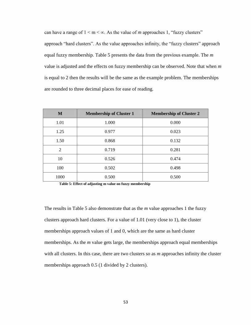
In this section, the effect of adjusting the m value is demonstrated. Recall that the m value
is the fuzzy exponent which indicates the degree of “fuzziness” of the clusters. The value
53
can have a range of 1 < m < ∞. As the value of m approaches 1, “fuzzy clusters”
approach “hard clusters”. As the value approaches infinity, the “fuzzy clusters” approach
equal fuzzy membership. Table 5 presents the data from the previous example. The m
value is adjusted and the effects on fuzzy membership can be observed. Note that when m
is equal to 2 then the results will be the same as the example problem. The memberships
are rounded to three decimal places for ease of reading.
M Membership of Cluster 1 Membership of Cluster 2
1.01 1.000 0.000
1.25 0.977 0.023
1.50 0.868 0.132
2 0.719 0.281
10 0.526 0.474
100 0.502 0.498
1000 0.500 0.500
Table 5: Effect of adjusting m value on fuzzy membership
The results in Table 5 also demonstrate that as the m value approaches 1 the fuzzy
clusters approach hard clusters. For a value of 1.01 (very close to 1), the cluster
memberships approach values of 1 and 0, which are the same as hard cluster
memberships. As the m value gets large, the memberships approach equal memberships
with all clusters. In this case, there are two clusters so as m approaches infinity the cluster
memberships approach 0.5 (1 divided by 2 clusters).

54
Calculating New Cluster Centers:
As with K-Means and Kohonen networks, the Fuzzy C-Means algorithm calculated the
clusters through an iterative process. In each step of the process, the data point
memberships are determined. Then these data points and cluster memberships are used to
determine new cluster centers via a weighted average approach. The formula for
calculating the new centers is given by Equation 11.
𝒄𝒌 = 𝒖𝒌𝒊
𝒎 𝒙𝒊 𝒏𝒊=𝟏
𝒖𝒌𝒊 𝒎 𝒏𝒊=𝟏
Equation 11
In this equation, the value of x is the nth
data point and the value of u is the cluster
membership of the nth
data point for cluster k. The value of m is the fuzzy exponent
described above. As already stated in the section on K-Means and Kohonen network
clustering, the starting points of the cluster centers impact the final cluster centers. In
addition to the starting point, the value of m also impacts the final clusters. To illustrate
this point, a brief example will be given using the Höppner, et. al data set from Table 1.
For this example, the starting points for the two centers will always be (0.8, 0.2) and (0.2,
0.8). The final center points for each value of m are provided in Table 6. Note that for
large values of m, there can be significant rounding error when using Equation 11.
Therefore, reproducing the results below will depend upon the floating point accuracy of
the software in use.

55
M Center 1 Center 2 Iterations Distance
K-Means (0.714, 0.333) (0.286, 0.667) 1 0.849
1.01 (0.714, 0.333) (0.286, 0.667) 1 0.849
1.25 (0.714, 0.333) (0.286, 0.667) 2 0.849
1.50 (0.710, 0.324) (0.290, 0.676) 4 0.548
2 (0.696, 0.304) (0.304, 0.696) 4 0.556
10 (0.603, 0.308) (0.397, 0.692) 17 0.436
100 (0.585, 0.301) (0.415, 0.699) 22 0.433
Table 6: Cluster Centers after convergence for different values of m.
From Table 6, it is observed that for small values of m the resulting center points after
convergence are close or identical to the center points obtained when using the K-Means
algorithm. This is as expected because as m approaches 1, cluster membership
approaches hard clustering. As the value of m increases, the number of iterations until
convergence increases and the distance between the cluster centers gets smaller.

56
METHODS
As was previously discussed, clustering is a tool that is widely used in the field of data
mining. There are two types of clustering, “hard” and “fuzzy”. Hard clustering limits
membership to one (and only one) cluster. Fuzzy clusters are a generalization of hard
clusters where a record may have partial membership (summing to 1) in one or more
cluster. In fact, hard clustering is a special case of fuzzy clustering. It has also been
discussed that although fuzzy clustering is widely used it is not implemented in the two
most widely used commercially available data mining programs: SAS Enterprise Miner
5.3 and SPSS Clementine 12. This section will describe approaches to approximate fuzzy
cluster membership using the already implemented hard clustering techniques.
Approximating Fuzzy Clusters Using Hard Cluster Techniques
Both SAS Enterprise Miner and SPSS Clementine have implemented hard clustering
techniques. These are based on K-Means clustering (and variations on K-Means
techniques), and Kohonen Self Organizing Maps. However, neither tool was designed for
easily extending the functionality for fuzzy clustering. This makes actual fuzzy clustering
impractical for most users.

57
The solution proposed in this document is to first determine the cluster centers using hard
clustering techniques that are already implemented. After these are determined, then
fuzzy membership functions will be employed on the back end to simulate fuzzy clusters.
This approach has the advantage of being simple to implement, thus making it accessible
to any person who is reasonably proficient in either tool. The disadvantage to this
approach is that the cluster centers that will be used will be most likely different from
those that would have been calculated had fuzzy clustering been used to derive the
centers. Referring back to Table 6, it is seen that for small values of m, the cluster centers
are similar. But for larger values of m, the clusters centers can be significantly different
from the hard clustering. Thus, the technique described in this research will be an
approximation of fuzzy clustering.
Extending SPSS Clementine to Include Fuzzy Membership
SPSS Clementine has a simple user interface that does not have or require any advanced
programming skills. Instead, all data mining functions from data transformation to model
development are encapsulated within graphical icons called “nodes”. A node insulates the
user from the mechanics of data manipulation and advanced statistics. The use of nodes
makes the tool more simple to use, but limits its flexibility. As such, it is not practical to
implement fuzzy membership using macros or a programming language. Instead, any
complex function such as fuzzy membership must be implemented within the graphical
user interface (GUI). This could pose a problem since the functionality to calculate fuzzy
membership could take many nodes. However, SPSS permits users to create complicated

58
work streams and then encapsulate them into a single super node. Thus, the user can have
a single node to function as a point of entry and exit for fuzzy membership. Because there
is no programming language to access, the user is required to make some minor changes
to the flow stream; but these are not difficult to execute. The flow stream in the following
section will generate fuzzy membership values. The code has been validated using both
published examples and hand calculated examples, which produced consistent results.
SPSS Fuzzy Clementine Fuzzy Membership Work Stream:
The fuzzy membership function is presented below in an SPSS Clementine work stream.
It is comprised of numerous nodes that are encapsulated within a single super node as is
shown in Figure 1. This super node can be copied into the clipboard memory and pasted
into other Clementine projects. This will make fuzzy membership functionality available
in any project where it is needed.
This super node assumes that clusters have already been generated using a hard clustering
technique such as K-Means or Kohonen networks. It also assumes that for each record in
a data set, a distance value has been calculated to each of the cluster centers. The nodes
contained within the super node of Figure 1will be described in greater detail.

59
Figure 1: SPSS Clementine Super Node for Fuzzy Membership Calculations
The super node of Figure 1 is expanded and shown in Figure 2. These are the nodes that
are contained within the super node. Among these, there are three super nodes that
encapsulate functions that are necessary to calculate fuzzy membership. The general
functionality of this flow diagram is as follows:
Copy distance values to standard variables for use within the flow stream
Set an m value (fuzzy exponent)
Calculate fuzzy membership values
Handle the special case that a record is directly on top of a cluster center (i.e. zero
distance).
Calculate the sum of the membership values
Normalize all of the membership values so that they sum to 1.0
Filter the unnecessary variables.
Figure 2: Flow Stream after the “Fuzzy Membership” super node was expanded.

60
The flow stream presented in Figure 2 assumes that the incoming records contain
variables that represent the distance from the each record to each cluster center. These
distance variables could have virtually any name. Therefore, these need to be copied to
distance values that use standardized names known to the nodes within this stream. The
purpose of the first node in the flow stream of Figure 2 (shown in Figure 3) is to allow
the users to copy their distance variables to the standardized names.
Figure 3: Node to initialize distances

61
When Figure 3 is expanded (shown in Figure 4), the user is presented with 25 derive
nodes which will derive 25 standard distance variables that will be used later in the flow
stream. This is one of the few places where the user needs to alter the Fuzzy Membership
super node. The limit to the number of clusters that this super node can handle, therefore,
is 25 (although using less is permitted). In most data mining applications, this should be
sufficient, but if more are needed then the user will need to add additional nodes to this
stream and will also need to make changes in subsequent nodes to take into account the
additional distance variables. The reason that there are 25 hard coded nodes in this stream
as opposed to a more generalized approach is that SPSS Clementine does not, in this
release, offer functionality for this type of generalization.
Figure 4: Generic Distance super node is expanded

62
In order for a user to copy their distance value to a generic variable, they must select the
appropriate node starting at 1 and increment by one for every additional distance variable.
The process of copying a distance value to a generic distance is presented in Figure 5. In
this example, it is assumed that the user has a distance variable called “KMDIST_1”.
This value is being copied to a value called “DIST_1”.
Figure 5: Copying user defined distance “KMDIST_1” to generic distance value “DIST_1”

63
It is unlikely that a user will have exactly 25 clusters from their hard cluster analysis.
More likely, they will have less than 25. In this case, the user must fill in the remaining
nodes with dummy values. The node is currently set so that the values are defaulted to a
value of 99. In the case where there are more than 25 clusters, then more nodes can be
added to this stream. However, the rest of the nodes in this Fuzzy Membership stream
will need to be updated to account for more than 25 clusters. Figure 6 gives an example
of filling in an extra node with a value of 99. A best practice would be to have all of the
values preset to 99, which would reduce the amount of work by the analyst.
Figure 6: Handling extra generic distances when there are less than 25 clusters
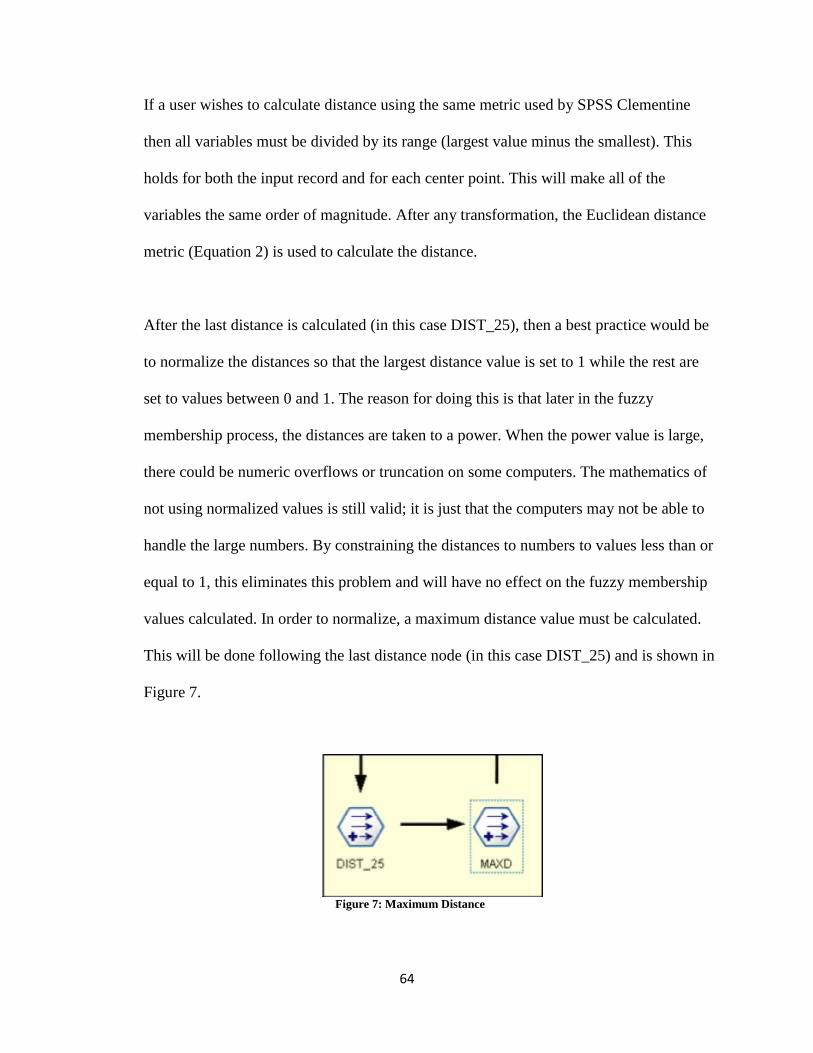
64
If a user wishes to calculate distance using the same metric used by SPSS Clementine
then all variables must be divided by its range (largest value minus the smallest). This
holds for both the input record and for each center point. This will make all of the
variables the same order of magnitude. After any transformation, the Euclidean distance
metric (Equation 2) is used to calculate the distance.
After the last distance is calculated (in this case DIST_25), then a best practice would be
to normalize the distances so that the largest distance value is set to 1 while the rest are
set to values between 0 and 1. The reason for doing this is that later in the fuzzy
membership process, the distances are taken to a power. When the power value is large,
there could be numeric overflows or truncation on some computers. The mathematics of
not using normalized values is still valid; it is just that the computers may not be able to
handle the large numbers. By constraining the distances to numbers to values less than or
equal to 1, this eliminates this problem and will have no effect on the fuzzy membership
values calculated. In order to normalize, a maximum distance value must be calculated.
This will be done following the last distance node (in this case DIST_25) and is shown in
Figure 7.
Figure 7: Maximum Distance

65
The calculation for determining the maximum distance inside of SPSS Clementine
requires the use of the max_n function as is shown in Figure 8. In this example, the user
is only using 5 of the 25 possible distance values. Therefore, the user must now include
the remaining 20 nodes, which requires user intervention. Notice that the distance
variables are enclosed in square brackets and separated by commas.
Figure 8: Maximum Distance Formula Inside of SPSS Clementine

66
After the maximum distance has been determined, a SPSS Clementine filler node is used
to normalize the distance values to 1. The process for this is given in Figure 9.
Figure 9: Normalize Distance to values ranging from 0 to 1
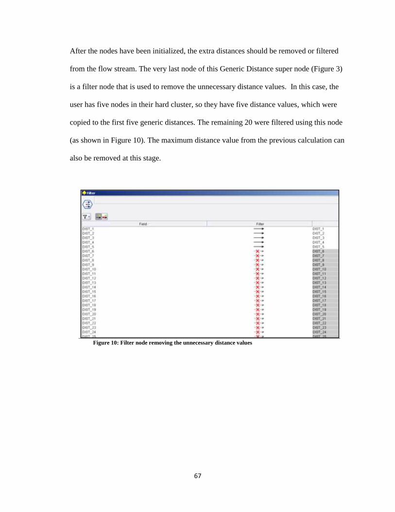
67
After the nodes have been initialized, the extra distances should be removed or filtered
from the flow stream. The very last node of this Generic Distance super node (Figure 3)
is a filter node that is used to remove the unnecessary distance values. In this case, the
user has five nodes in their hard cluster, so they have five distance values, which were
copied to the first five generic distances. The remaining 20 were filtered using this node
(as shown in Figure 10). The maximum distance value from the previous calculation can
also be removed at this stage.
Figure 10: Filter node removing the unnecessary distance values

68
Referring back to Figure 2, the next step in the flow diagram is to set the fuzzy exponent,
m. As has already been discussed, this variable must take on a value greater than 1. The
closer the value is to 1, the more the cluster memberships resemble hard clusters. The
greater the value, the more the clusters become fuzzy. Typically, researchers tend to set
this value to 2. The derive node for the fuzzy exponent is given in Figure 11. This node is
the second node that the user will need to adjust.
Figure 11: Setting the fuzzy exponent value (any value greater than 1).

69
The next step in the flow diagram of Figure 2 does the actual calculations for fuzzy
membership. The node, shown in Figure 12 is a super node that encapsulates several
functions. The super node is expanded in Figure 13.
Figure 12: Node to calculate fuzzy membership
The expanded node determines the preliminary fuzzy membership values for each record
in a data set. These functions do the calculations described in Equation 5 through
Equation 10. The first node in this stream uses a derive node to calculate the fuzzy power
value using Equation 5. There is no need for a user to adjust this node.
Figure 13: Expanded super node to calculate preliminary fuzzy memberships

70
Referring to Equation 7, it is necessary to find each distance taken to the fuzzy power.
The derive node of Figure 14 accomplishes this task with multiple calculations of all of
the distance variables. This node has all of the distance variables from 1 through 25 hard
coded. If the user has filtered any of these values earlier in the stream, then they appear in
the color red inside of this node and are ignored. There is no reason that a user should
alter this node unless the user has more than 25 distance values. In such a case, the user
must add the additional variables to this node.
Figure 14: Determine the distance values taken to the fuzzy power (first part of Equation 7)

71
The subsequent node (seen in Figure 15) will sum all of the values created in Figure 14.
This node looks for variables that match a specific pattern (names starting with
“Power_Dist_”). Because this node matches variable naming patterns, it will never need
to be adjusted by the user for any reason (such as having too many or too few distance
values). The output of this node will be the result of Equation 7.
Figure 15: Sum all of the distance values taken to the fuzzy power (Equation 7)

72
The preliminary fuzzy membership for each record to each of the clusters is calculated
using the node in Figure 16. The output of this node is result of Equation 8. If the user
has filtered the distance values so that there are less than 25, then there should be no
reason to alter this node. If the user has added distance values, then this node will need to
be updated to reflect these changes.
Figure 16: Calculate the fuzzy membership (value found in Equation 8)

73
Referring back to Figure 2, the next node in the flow stream is titled Handle Zero
Distances (Figure 17). This is an error checking node that handles the special case where
one or more of the distances are zero. The chance that a data point will fall exactly on a
cluster center is unlikely, but not impossible. As such there will be divisions by zero in
some of the equations. This super node will perform the logic to handle that condition.
This super node will also handle the case where two distances are zero. This is unlikely to
ever occur, but might be possible as a result of rounding or in the remote chance that the
clustering algorithm places two centers on the same point.
Figure 17: Handle zero distances

74
The nodes contained within the super node of Figure 17 are shown in Figure 18. These
nodes perform the following functions respectively. First, the distances are checked to see
if any are null values. This would indicate a division by a zero distance which occurs
only when a record is directly on top of a cluster center. If one or more of the clusters are
has a null value, then they are set to a membership of 1 while the rest of the fuzzy
memberships are set to zero.
Figure 18: Nodes within the Handle Zero Distances super node

75
The first node of the stream in Figure 18 is shown in Figure 19. This examines each of
the fuzzy membership values from Figure 16. If any of them are null values, then that
indicates that it was on a cluster center. If a user filtered any of the distance values so that
there are less than 25, then this node will be able to handle this case without any
intervention. If the user has increased the number of distance values beyond 25, then this
node will need to be updated to account for the additional values.
Figure 19: Determine if a Fuzzy Membership is a null value (indicating that it is on a cluster center)

76
The values calculated in Figure 19 are added together in the next node (Figure 20). If the
sum is greater than zero, then the record is on one of the cluster centers. Note that it
theoretically possible (though unlikely) that a clustering algorithm will place two clusters
so close together that they are essentially the same point. Thus it will be unlikely that this
value will ever exceed 1, but this flow diagram will still be able to handle this. The node
in Figure 20 matches variables that start with “NULL_U_POWER_DIST” and has no
variables hard coded. Therefore, there is no reason for a user to ever alter this code
regardless of whether distance variables are added or deleted.
Figure 20: If the Sum of NULL_U_POWER_DIST values is greater than 0, the record is on a cluster
center.

77
In Figure 21, the fuzzy memberships are adjusted to account for a record being on top of
a cluster center. The logic of this node checks to see if the Null Flag (from Figure 20) is
true. If it is then the record is on a cluster center. Thus, all of the points that are NOT set
to null are not on a cluster center. These must then be set to a membership of 0. This node
has hard coded values, so if the distance values filtered to less than 25 then nothing needs
to be done. If values are added to exceed 25, then this node will need to be updated.
Figure 21: If a record is on a cluster center, set all the other membership values to zero.

78
Finally in Figure 22, if the Null Flag (from Figure 20) is set to true, then all of the
membership values set to null will be set to 1. This is because they are exactly on top of a
cluster center (thus there is a division by zero). Again, this node will handle the case
where two or more cluster centers are so close to one another that they are virtually the
same point, but in practice this is unlikely to occur. This node has hard coded values, so if
the user filters the distance value to under 25 variables, then no change is necessary.
Increasing the number of nodes beyond 25 requires adjustments.
Figure 22: If the Null Flag is true (record is on a cluster center) set the null value to 1 (it is on top
of the center).

79
The next node sums all of the fuzzy membership values together (shown in Figure 23).
Theoretically the values should sum to 1, but due to round off error this might be slightly
different from 1. Summing the memberships allows for adjusting so that all membership
values can be normalized. Figure 23 should not need to be altered by the user. This node
performs the function described in Equation 9.
Figure 23: Sum the fuzzy membership values together (see Equation 9)

80
In Figure 24, all of the fuzzy membership values are divided by the sum so that they are
normalized to 1 as is described in Equation 10. The user should not need to alter this node
unless more than 25 distances values are used.
Figure 24: Divide by the sum of the memberships in order to normalize the membership variables
(Equation 10)
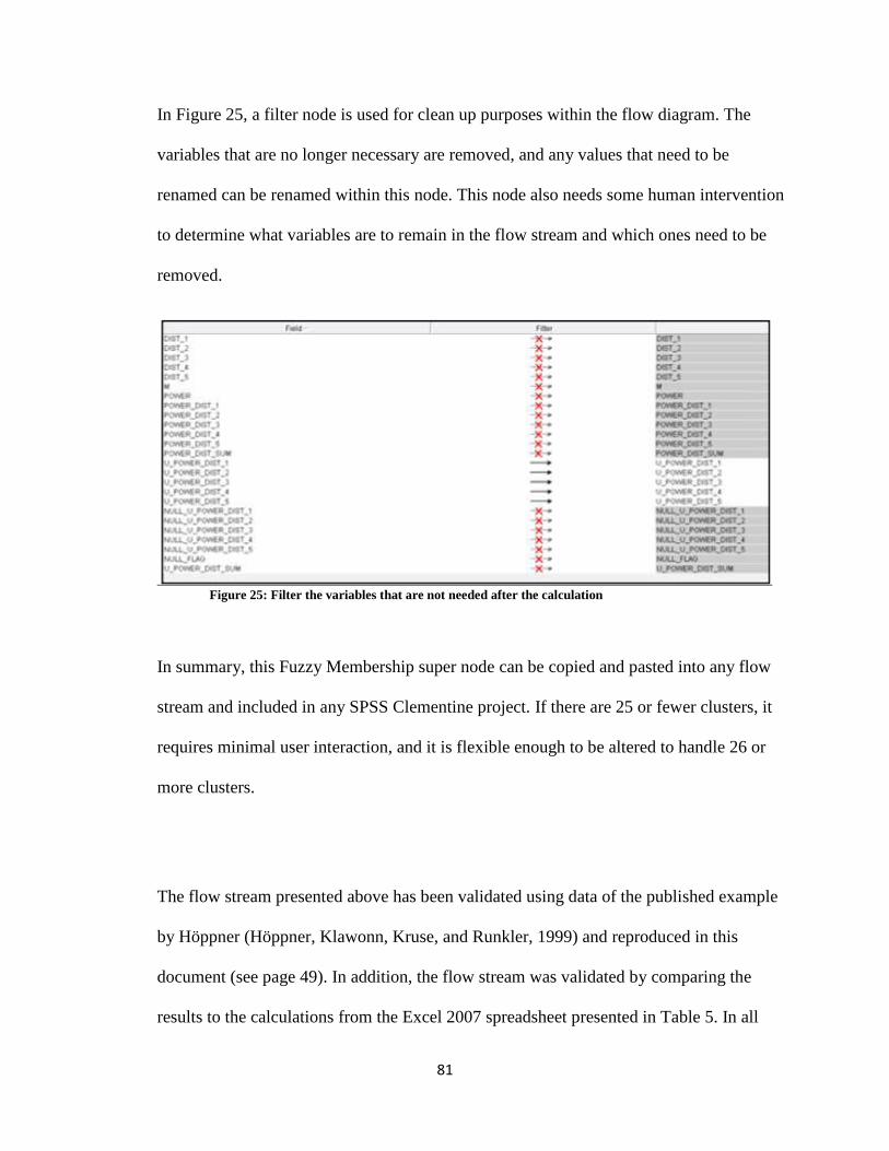
81
In Figure 25, a filter node is used for clean up purposes within the flow diagram. The
variables that are no longer necessary are removed, and any values that need to be
renamed can be renamed within this node. This node also needs some human intervention
to determine what variables are to remain in the flow stream and which ones need to be
removed.
Figure 25: Filter the variables that are not needed after the calculation
In summary, this Fuzzy Membership super node can be copied and pasted into any flow
stream and included in any SPSS Clementine project. If there are 25 or fewer clusters, it
requires minimal user interaction, and it is flexible enough to be altered to handle 26 or
more clusters.
The flow stream presented above has been validated using data of the published example
by Höppner (Höppner, Klawonn, Kruse, and Runkler, 1999) and reproduced in this
document (see page 49). In addition, the flow stream was validated by comparing the
results to the calculations from the Excel 2007 spreadsheet presented in Table 5. In all

82
cases, the flow stream produced the same results. This suggests that the implementation
in SPSS Clementine is correct.
Example of SPSS Clementine Model:
The following example will provide a brief, step-by-step tutorial on using the Fuzzy
Membership super node described above. This example reuses the Wisconsin Breast
Cancer Data Set. Again, nine clusters will be generated using the variables Bland
Chromatin and Clump Thickness.
Step 1: Create the Clusters Using Clementine:
Read in a data set, sorted in ascending order by ID number, from the file and filter out the
unnecessary fields so that the clustering will be conducted on the Bland Chromatin and
Clump Thickness variables (see Figure 26). The K-Means node was set to generate nine
clusters, the same number used for the Kohonen network example.
Figure 26: Read in data for clustering
The stream is executed and SPSS Clementine generates a model node that needs to be
attached to the flow stream. During the next step, distance values will be calculated. For

83
this example, it is assumed that the user wishes to use the same method for calculating
distances that Clementine uses, although this is not a requirement. The Clementine
method requires a division by the range of a variable, which can be determined by a
statistics node. Therefore, a statistics node is added to the flow stream and the range box
is selected within the node (this is not shown). The new flow stream is shown Figure 27.
When the statistics node is executed, it is learned that both Bland Chromatin and Clump
Thickness have range values of 9 (maximum values of 10 and minimum values of 1).
Figure 27: Adding a statistics node and the K-Means output to the stream
When the K-Means output node is examined, it is seen that Clementine gives information
on the cluster centers for all nine of the clusters (see Figure 28). For the sake of brevity,
only the first cluster center is expanded. From this, it is seen that the cluster center is at:
Bland Chromatin 2.256
Clump Thickness 4.268

84
When all nine of the clusters are expanded, then all of the center points can be
ascertained. These will be used in the next section for determining the distance from a
record to each of the centers.
Figure 28: Output of the K-Means Node
Step 2: Calculate Distance To Each Cluster:
Because there are nine clusters, nine distances must be calculated. These are determined
by derive nodes within Clementine. To do this, attach nine derive nodes in succession off
of the K-Means output node. For clarity, the nine distance variables will be named D1
through D9 with each of the distances corresponding to the appropriate cluster (see
Figure 29).
Figure 29: Nine Distance Calculation Nodes attached to the K-Means output node.

85
Recall that the range values for Bland Chromatin and Clump Thickness were found to be
9 and that the center point for the first cluster was found to be:
Bland Chromatin 2.256
Clump Thickness 4.268
Then the distance value in the first node is found using with the formula in Figure 30.
The calculations for the remaining distance values are determined in the same manner.
Figure 30: Distance calculation for the first cluster.

86
Step 3: Calculate the Fuzzy Memberships.
After the distance memberships are calculated, the fuzzy membership node is attached to
the end of the distance nodes (as is shown in Figure 31).
Figure 31: Attach the fuzzy membership super node
Some simple changes to the super node need to be done in order to configure it to
calculate the fuzzy memberships. In this case, the only required change is to alter the
distance super node (previously shown in Figure 3). When that super node is expanded,
the distance nodes are shown as seen in Figure 4. This is where all of the changes need to
be affected. For the first node, DIST_1, the formula is altered so that the value of D1 is
copied onto DIST_1 (see Figure 32).
Figure 32: DIST_1 is altered to be D1 from the flow stream

87
This same procedure is repeated for the remaining distance values. The filter node can be
used to remove any unwanted variables. The value for m is defaulted to 2, but that can be
altered if desired. At this point, all the necessary changes have been accomplished to
calculate fuzzy membership. Nodes can be attached to the Fuzzy Membership super node
and these values can be used in subsequent calculations and analysis.
The previous example could have easily been applied to the Kohonen clusters and Two
Stage Clustering nodes by following the exact same procedure except for the fact that
different clustering nodes are used. An example using the Kohonen network will be done
in the section on SAS Enterprise Miner.
Discussion of SPSS Clementine Model:
The flow stream presented is a simple and accurate way to create fuzzy membership
values. It is simple to use and to incorporate into an SPSS Clementine flow stream. The
only requirement is that the user provides distance measures to clusters. In fact, the
clusters are even optional as any distance metric can be provided to the flow stream and a
fuzzy membership will be calculated. The user only needs to interact with a few of the
nodes within the flow stream, the rest are automatic.
However, because SPSS Clementine is geared more towards being a GUI model building
tool, it does not rely on a native programming language. As such, it is difficult to
introduce cluster centers and distance values into the flow stream in an automated
fashion. Therefore, if the distance values are not already in the data set then users must

88
generate them using a derive node. This is not difficult if there are only a couple of
distances. However, as the number of distances grows then it becomes progressively
more difficult and prone to typographical error. Another disadvantage to this technique is
that it requires that there be an upper bound to the number of distances. In this case, it
was arbitrarily set to 25. If the user wishes to include more, then it will require adjusting
many of the nodes along the path. Of course, these changes are simple but any
intervention by a programmer carries with it a chance of error. So in that respect this
approach does carry some risk. An addition disadvantage of this flow stream is that it is
implemented inside of the GUI as opposed to a programming language. A user is
therefore tied to the SPSS Clementine GUI. If SPSS Clementine changes their GUI, it is
conceivable that this program may no longer function properly. Despite these
disadvantages, the flow stream is still an effective method of incorporating fuzzy
membership into SPSS Clementine projects.
Extending SAS Enterprise Miner to Include Fuzzy Membership
The SAS Enterprise Miner program is similar to SPSS Clementine in that it is a GUI
based data mining tool. It has an additional advantage that it can access and execute SAS
programming language code. Because of this functionality, it is possible to extend
Enterprise Miner with far less effort. The advantage to this approach is that the code will
be considerably more flexible than a GUI interface. Also, it is not tied to a particular
program so that if the GUI changes significantly, this code will still execute. Also, the
code can execute outside of Enterprise Miner such as in a mainframe or data warehouse.
The disadvantage to this approach is that it does require some knowledge of the SAS

89
programming language. This is not necessarily difficult to learn in most cases, but it still
may be a barrier for some users. Of course, there is always an option to build a flow
diagram inside of Enterprise Miner that is similar to the Clementine approach in that it
relies only on nodes and no coding. However, this would still require some SAS
Programming constructs in the work flow, so this approach would only add complexity
and not give any advantages of using the simpler program.
SAS Enterprise Miner Fuzzy Membership Work Stream:
The SAS Enterprise Miner approach to Fuzzy Membership calculation makes use of a
SAS Macro program which converts distance measures to fuzzy membership values.
Because it transforms distance values directly, the SAS Macro is similar to the SPSS
Clementine work flow in that it does not actually require clusters to be calculated, only
distances. This means that this macro can be used for other applications as well as fuzzy
cluster membership. Note that the distance metric used in the K-Means node is the
distance squared value. Therefore, the macro takes the square root of all distances before
doing any calculations. If the user is providing the distance metrics, then they must be
squared for consistency before passing them into the macro.
There are two requirements for the use of this macro. First, it must be contained within a
SAS data statement. Second, the distances must be contained within an array variable.
As with the SPSS Clementine approach, this macro code has been validated using both
published examples and hand computations and the results are consistent. The macro is
presented in Table 7, and the logic will be discussed in the text following the table.

90
%macro fuzzyCluster( DARRAY, UARRAY, SIZE=20, M=2 );
array &UARRAY. &UARRAY.1-&UARRAY.&SIZE.;
array D&UARRAY.[&SIZE.] _temporary_;
length POWER 8.; drop POWER;
length DISTSUM 8.; drop DISTSUM;
length DISTFLAG 8.; drop DISTFLAG;
length i 8.; drop i;
length MAXD 8.; drop MAXD;
POWER = 2/(&M.-1);
MAXD = -1;
do i = 1 to &SIZE.;
D&UARRAY.[i] = sqrt(&DARRAY.[i]);
if D&UARRAY.[i] > MAXD then MAXD = D&UARRAY.[i];
end;
do i = 1 to &SIZE.;
D&UARRAY.[i] = D&UARRAY.[i] / MAXD;
end;
DISTSUM = 0;
do i = 1 to &SIZE.;
DISTSUM = DISTSUM + D&UARRAY.[i]**POWER;
end;
do i = 1 to &SIZE.;
&UARRAY.[i] = 1 / ( (D&UARRAY.[i]**POWER)*DISTSUM );
end;
DISTFLAG = 0;
do i = 1 to &SIZE.;
if missing( &UARRAY.[i] ) then DISTFLAG = 1;
end;
if DISTFLAG > 0 then do;
do i = 1 to &SIZE.;
if missing( &UARRAY.[i] ) then
&UARRAY.[i] = 1;
else
&UARRAY.[i] = 0;
end;
end;
DISTSUM = 0;
do i = 1 to &SIZE.;
DISTSUM = DISTSUM + &UARRAY.[i];
end;
do i = 1 to &SIZE.;
&UARRAY.[i] = &UARRAY.[i] / DISTSUM;
&UARRAY.[i] = round( &UARRAY.[i], 0.001 );
end;
%mend;
Table 7: SAS Macro to calculate Fuzzy Membership
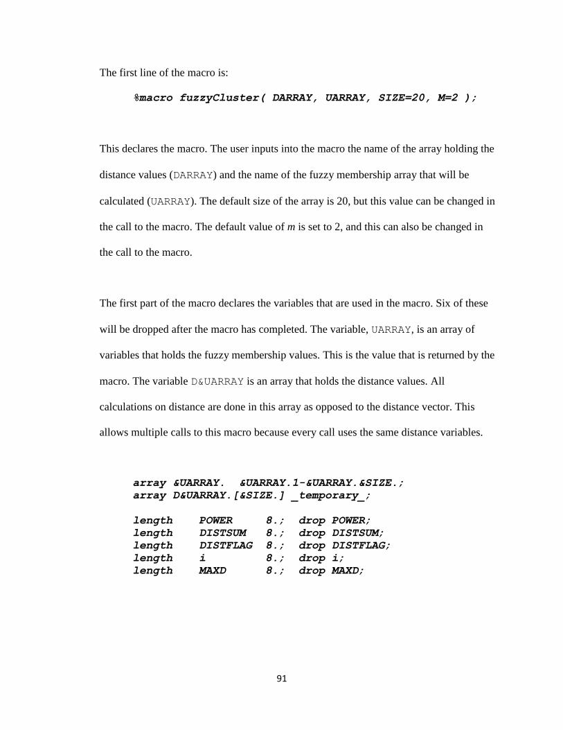
91
The first line of the macro is:
%macro fuzzyCluster( DARRAY, UARRAY, SIZE=20, M=2 );
This declares the macro. The user inputs into the macro the name of the array holding the
distance values (DARRAY) and the name of the fuzzy membership array that will be
calculated (UARRAY). The default size of the array is 20, but this value can be changed in
the call to the macro. The default value of m is set to 2, and this can also be changed in
the call to the macro.
The first part of the macro declares the variables that are used in the macro. Six of these
will be dropped after the macro has completed. The variable, UARRAY, is an array of
variables that holds the fuzzy membership values. This is the value that is returned by the
macro. The variable D&UARRAY is an array that holds the distance values. All
calculations on distance are done in this array as opposed to the distance vector. This
allows multiple calls to this macro because every call uses the same distance variables.
array &UARRAY. &UARRAY.1-&UARRAY.&SIZE.;
array D&UARRAY.[&SIZE.] _temporary_;
length POWER 8.; drop POWER;
length DISTSUM 8.; drop DISTSUM;
length DISTFLAG 8.; drop DISTFLAG;
length i 8.; drop i;
length MAXD 8.; drop MAXD;

92
The next section of code calculates the power value using the m value that was passed
into the macro. This code performs the calculation described in Equation 5.
POWER = 2/(&M.-1);
In the next section of code, the square root of the distance is copied into the temporary
distance array. The reason that the square root is calculated is that enterprise miner stores
the distance as the distance square. Furthermore, during the copying process, the macro
determines the maximum distance value. This will be used in the next segment of code.
MAXD = -1;
do i = 1 to &SIZE.;
D&UARRAY.[i] = sqrt(&DARRAY.[i]);
if D&UARRAY.[i] > MAXD then MAXD = D&UARRAY.[i];
end;
Now each distance is divided by the maximum distance from the previous section. The
reason for doing this is that when m is close to 1, then the POWER value gets large. This
can lead to some very large values when taking distances to a large power. The
mathematics will still be correct, yet from a practical stand point, a computer may face
rounding and truncation issues. Thus, dividing the distances by the maximum value will
normalize the values to between 0 and 1.
do i = 1 to &SIZE.;
D&UARRAY.[i] = D&UARRAY.[i] / MAXD;
end;

93
In the next segment of code, the power distance is calculated as per the formula given in
Equation 7. This value is used in the next segment of code.
DISTSUM = 0;
do i = 1 to &SIZE.;
DISTSUM = DISTSUM + D&UARRAY.[i]**POWER;
end;
The preliminary cluster membership is determined as per Equation 8.
do i = 1 to &SIZE.;
&UARRAY.[i] = 1 /((D&UARRAY.[i]**POWER)*DISTSUM;
end;
This section of code checks whether or not a record resides on top of a cluster center. In
such a case, there would be a division by zero in the calculation in the previous section of
code, which is represented by a missing value in SAS. Therefore, this section of code
iterates through all of the preliminary fuzzy memberships. If any of them are missing, the
DISTFLAG is set to true.
DISTFLAG = 0;
do i = 1 to &SIZE.;
if missing( &UARRAY.[i] ) then DISTFLAG = 1;
end;

94
This code executes if and only if the DISTFLAG from the previous section is true, which
occurs only if a record is on a cluster center. If the code executes, then it will set the
fuzzy membership to 1 if it is missing and 0 otherwise.
if DISTFLAG > 0 then do;
do i = 1 to &SIZE.;
if missing( &UARRAY.[i] ) then
&UARRAY.[i] = 1;
else
&UARRAY.[i] = 0;
end;
end;
All of the fuzzy membership values are summed together. In theory, they should sum to 1
but it is possible that rounding error may prevent this. By finding the sum, this value can
be used to scale the fuzzy memberships so that they do sum to 1. This code implements
the formula described by Equation 9.
DISTSUM = 0;
do i = 1 to &SIZE.;
DISTSUM = DISTSUM + &UARRAY.[i];
end;
Finally, the formula from Equation 10 is implemented in the following code. It will
normalize all of the membership values to 1. The fuzzy memberships are then rounded to
three decimal places to make displaying more readable and for making it easier to hand
check results. This is purely for convenience and is not mathematically necessary.
do i = 1 to &SIZE.;
&UARRAY.[i] = &UARRAY.[i] / DISTSUM;
&UARRAY.[i] = round( &UARRAY.[i], 0.001 );
end;

95
The SAS code presented above has been validated using data of the published example
by Höppner (Höppner, et al., 1999) and reproduced in this document (see page 49). In
addition, it was validated by comparing the results to the calculations from Excel 2007
presented in Table 5. In all cases, the flow stream produced the same results. This
suggests that the implementation in SAS Enterprise Miner is correct.

96
Example 1 of SAS Enterprise Miner Model:
The following example will provide a brief, step by step tutorial on using the Fuzzy
Membership SAS macro in a stand-alone SAS program. This example will demonstrate
that it is not required to have clusters or SAS Enterprise Miner in order to use this macro.
In addition, the macro is versatile enough that it can be called multiple times within the
same program using different m values. In this example, the data is the same data used in
Table 5, except that the equation will only be run for m=1.5 and m=2. The program is
presented below in Table 8. The code is explained following the table.
%include "C:\SASMACRO\UTILITY\math_fuzzycluster.sas";
data TEMP;
input X Y;
X = X/7;
Y = Y/7;
cards;
5 4
;
run;
data TEMP;
set TEMP;
array C[2] _temporary_;
C[1] = (X-0.69598)**2 + (Y-0.30402)**2;
C[2] = (X-0.30402)**2 + (Y-0.69598)**2;
%fuzzyCluster( C, UARRAYa, SIZE=2, M=1.5 );
%fuzzyCluster( C, UARRAYb, SIZE=2, M=2.0 );
run;
proc print data=TEMP;
run;
Table 8: SAS Fuzzy Membership Example 1

97
This first segment of code references the SAS Macro that was presented Table 7. The
code loads the macro “math_fuzzycluster.sas” into the SAS program.
%include "C:\SASMACRO\UTILITY\math_fuzzycluster.sas";
This next segment of code will read in one record and divide each value by 7. This will
give the same input values as the data used for the calculations in Table 5. Note that if it
is desired, more than one record may be included in the “cards” section, but in this case
only one record is being used.
data TEMP;
input X Y;
X = X/7;
Y = Y/7;
cards;
5 4
;
run;
The following data step calculates the distance from the record to the cluster center
points. These were also given in the example referenced by Table 5. Notice that the
distance values are actually the distance squared. This is because the macro requires a
distance squared value instead of the distance value. The distance values are stored in a
SAS array value that is named “C”.
data TEMP;
set TEMP;
array C[2] _temporary_;
C[1] = (X-0.69598)**2 + (Y-0.30402)**2;
C[2] = (X-0.30402)**2 + (Y-0.69598)**2;

98
The next two lines references the SAS Macro. Notice that there are two calls to the
macro. In the first call, the value for m was 1.5 and in the second the value for m was 2.
In the call to the macro, the first argument tells the macro that the array holding the
distance is called “C”. The second argument tells the macro what to name the array that
holds the fuzzy membership. In the first call, the membership value will be called
“UARRAYa” and in the second it will be called “UARRAYb”. Finally, the values for m are
set at 1.5 and 2.0 respectively.
%fuzzyCluster( C, UARRAYa, SIZE=2, M=1.5 );
%fuzzyCluster( C, UARRAYb, SIZE=2, M=2.0 );
Finally a call to a print procedure is made to display the results.
proc print data=TEMP;
run;
The results of the program given in Table 8 are:
X Y UARRAYa1 UARRAYa2 UARRAYb1 UARRAYb2
0.71429 0.57143 0.86751 0.13249 0.71901 0.28099
These results are consistent the result presented in Table 5 for the m values of 1.5 and
2.0. Therefore, this example has demonstrated the use of the SAS Macro that calculates
fuzzy membership. This macro requires distances to be stored in an array and calls to the
macro to be made from within a SAS data step.

99
Example 2 of SAS Enterprise Miner Model:
In the next example, SAS Enterprise Miner 5.3 will be used to generate clusters for the
Wisconsin Breast cancer data set on the Bland Chromatin and Clump Thickness
variables. In the SPSS Clementine example, the K-Means algorithm was used to cluster
so in this case the clustering algorithm will be the Kohonen network method for the sake
of illustration. However, as with SPSS Clementine, the choice of clustering algorithm is
irrelevant to calculating fuzzy membership. The work flow for generating the Kohonen
network clusters is given in
Figure 33. In the flow, the records are read and then transformed via standardization (Z-
Score Transform) which is calculated by subtracting the mean and then dividing by the
standard deviation. The records are then used by the Kohonen network node for
clustering. It was arbitrarily decided that the Kohonen network architecture would be a 3
by 3 as done earlier.
Figure 33: Learning the Kohonen/SOM Clusters
In SAS Enterprise Miner, nodes generate SAS programming language code, which can be
used either inside a work stream or outside of Enterprise Miner. The reason for this
feature is that it allows users to create models within Enterprise Miner and to score data
outside of Enterprise Miner such as in a mainframe or a data warehouse. This code is

100
necessary to create fuzzy memberships, where a SAS code node must be added to the
work stream as shown in Figure 34.
Figure 34: SAS Code node added to the stream
The initial code for the SAS code node is presented in Figure 35. The “%include” line at
the top is a link to the SAS macro that calculates fuzzy membership. The data step
accepts the data from the previous node (the Transform Variables node) and creates a
data set that can be exported to subsequent nodes. SAS Enterprise Miner makes use of
predefined macro variables “&EM_EXPORT_TRAIN.” and “&EM_IMPORT_DATA.” to
refer to the incoming and exported data. If this code is to run outside of Enterprise Miner,
these macro variables would be changed to data set names. Now the SAS code from the
Kohonen network must be added to this SAS code node.

101
Figure 35: Initial SAS Code
Accessing the code from the Kohonen node is a simple process. First, right mouse click
on the Kohonen node and select RESULTS. Go to the View option on the menu bar and
navigate to the SAS Code as shown in Figure 36. This will open a window containing
score code.
Figure 36: SAS Code from the Kohonen node

102
The SAS code from the window is shown in Figure 37. This can function as a stand-alone
SAS data step that will accept the standardized variables from the previous node and
place them in the appropriate Kohonen network cluster. To access this code, the user
must use the “control-a” key stroke to select all of it. Then the user must use the “control-
c” to copy the code to the memory.
Figure 37: Kohonen node score code

103
The code is then pasted into the SAS code node from Figure 35, immediately after the
line that says:
set &EM_IMPORT_DATA.;
See Figure 38 to see how the code appears.
Figure 38: Kohonen score code added to the SAS Code node
This code is now a complete data step that can put records into an appropriate cluster. It
is a simple matter to add calls to the fuzzy membership routine. First, the user must scroll
through the code until the array declaration of the distance variable is found. The code
should be located near the top and will be declared with an “array” statement. It will
most likely be a _temporary_ variable, but that could change in later releases of
Enterprise Miner. In this example, as is shown in Figure 39, the distance variable is called
“SOMvads” and it is an array of length 9. This is all that is needed for fuzzy membership
calculation.

104
Figure 39: Array of distance variables is declared
Now go to the very end of the code, just before the “run” command, and enter the call to
the SAS macro. The user must enter the name of the distance variable (“SOMvads”) and
the length of the array which is 9. The user must give a name to the array that holds the
fuzzy membership values. In this case it is “UARRAY”. Finally, the user must supply an m
value, in this example it is set to m=2. The call to the fuzzy membership macro is shown
below in Figure 40. As with the previous example, the user is not limited to one call to
this macro. The user may make several calls with different m values.
Figure 40: Call to the Fuzzy Cluster Macro

105
After this node, the cluster membership value of the Kohonen network and the fuzzy
membership values will be added to the record. These can be used as inputs into other
models, such as trees, regressions, or neural networks. Figure 41 gives an example of
how the fuzzy membership might be incorporated in a regression model.
Figure 41: Adding a modeling node after computing fuzzy membership
In summary, fuzzy membership can be incorporated in Enterprise Miner using SAS
Macros. This can be done with a considerable amount of programming flexibility, and it
can be applied to hard clustering techniques such as K-Means and Kohonen networks.
The use of this technique is not limited to clustering, and it can be applied to any distance
measure as was seen in the first example of this section.
Discussion of SAS Enterprise Miner Model:
The technique that was described in the above section is an effective method for
incorporating fuzzy membership into SAS Enterprise Miner. This technique has many
attractive features which could prove advantageous in an application. The most useful
feature is that it is based on the SAS Programming language. Thus it can be used to
develop models from within Enterprise Miner, but it can run outside of it such as in a
mainframe or data warehouse. Another advantage is that the user can make multiple calls
to the macro in succession. This is convenient and can allow the users to find the best m

106
value for their application. Another useful feature of this technique is that it is flexible
enough to use any distance metric. The distance value does not necessarily need to relate
to a cluster: it could be any distance such as driving distance to a grocery store. For cases
where there are cluster memberships, the macro call is simply appended to the end of the
data step generated by Enterprise Miner. This saves the user time and effort of needing to
calculate distance; also, when the distance formula is written by Enterprise Miner then
there is less chance of human error.
The one major drawback to this technique is that it does require some knowledge of SAS
programming. Although SAS is not a difficult language, this could prevent a GUI
preferring individual from using the macro.
Comparison of the Two Approaches
The previous sections described two methods for calculating fuzzy membership from
hard clusters. One approach used SPSS Clementine and the second used SAS Enterprise
Miner. Both approaches were shown to be effective and practical, but there are different
advantages and disadvantages to each. This section will summarize these tradeoffs.
The SPSS Clementine approach is a purely GUI methodology that requires no knowledge
of advanced programming or macros. The user can copy the super node and paste it into
the diagram directly. It is simple to use. However, there are several disadvantages to this
approach. First, because this is strictly a GUI approach, the user is tied to the SPSS

107
Clementine environment. Also, the lack of a programming language can make
calculations cumbersome when dealing with a large number of clusters or complicated
distance formulas, which will need to be hand coded inside a series of SPSS Clementine
derive nodes. Also, the user must actually alter nodes within the super node flow stream
to account for the number of clusters that will be used. This is not difficult, but the more
human intervention that is required the more likely is the chance of an error occurring.
Another drawback of this approach is that each use of the fuzzy membership super node
is self contained. Therefore, if a user employs this node numerous times and then makes a
change (perhaps a bug fix) then every use of the super node must be hunted down and
corrected. This is yet again another case where errors may be introduced. Despite the
difficulties that may arise, this is a reasonably simple solution to calculating fuzzy
memberships, but it is less flexible and can be more prone to human error.
The SAS Enterprise Miner approach is purely a programming approach. As such, it can
be executed from either within or outside of the SAS Enterprise Miner. It is flexible and
easily adjusts to any number of clusters or distance metrics. In addition, any changes to
the macro will instantly be realized by all other programs using it. The disadvantage to
this technique is that it requires SAS programming skills and the use of SAS code inside
the Enterprise Miner flow stream. For example, after the user identifies the hard clusters,
then the user must generate the stand-alone SAS code. The SAS macro to calculate fuzzy
membership is added to the bottom of this stand-alone code. This is less intuitive than a
GUI approach, but does offer more flexibility. For example, the use of the macro allows
for multiple calls. Therefore, different fuzzy memberships can be calculated using

108
different m values. But as stated before, the use of this macro does require some degree of
skill and sophistication that the user may not possess. This could ultimately act to
discourage its use for some users. In summary, the SAS Enterprise Miner approach is
highly flexible but requires knowledge of both the SAS programming language and SAS
macros.
Accuracy Improvement of Using Fuzzy Clusters Instead of Hard Clusters
In this section it is demonstrated that using fuzzy membership can yield better results
than hard cluster memberships. This is done by presenting a model and showing that
incorporating fuzzy membership increases accuracy, where accuracy is measured by
increase in profit realized.
The purpose of this demonstration is to satisfy the reader that fuzzy memberships are a
viable data mining technique. It is important to note that even if fuzzy memberships do
improve accuracy in this particular example, this does not imply that fuzzy memberships
are always better than hard memberships. There are times that hard clusters are a better
choice and there are times that fuzzy memberships are better. It is only suggested that the
reader consider fuzzy membership along with other data mining techniques when
building predictive models or conducting data analysis.
The data set used for this example is the KDD Cup data set from 1998 (Parsa and Howes,
1998). The purpose of this data set is to determine which person will donate to a national

109
veterans’ organization after being sent a solicitation. The donors are free to donate any
amount of money or no money at all. It costs the organization $0.68 to send a letter. The
goal is to maximize the profits.
For this illustration, a simple hard clustering model is applied to the data. Next, various
fuzzy membership models are applied to the same data. The profits realized for each
model are compared. Note that it is not our purpose to develop an optimal model for this
illustration, just a reasonable one that uses only clusters.
SAS Enterprise Miner 5.3 is used for this analysis. The clustering approach is a Kohonen
network with four rows and four columns (16 clusters total). The work flow for this
analysis is presented below in Figure 42.
Figure 42: Flow Diagram for KDD Cup analysis
For the clustering, all of the variables were standardized (Z-Score). This put all of the
variables on an equal weighting. The input variables used for the clustering are described
below.
INCOME – This is a categorical variable from 1 to 7. A value of 1 indicates a low
income and a 7 is a high income. Some of these values were missing, and these were
imputed using decision trees.

110
WEALTH1 – This is a categorical variable from 0 to 9 with zero being the lowest and 9
being the highest. Some of these values were missing, and these were imputed using
decision trees.
TOTAL NUMBER OF GIFTS – This is the total number of times a donor gave a gift.
TOTAL AMOUNT – This is the total amount of money donated by the donor.
TIME SINCE LAST DONATION – This is the number of months since the last time the
person donated. This variable was derived using the time the data set was created (June of
1997) and the date of the last donation.
The training data set that was provided was used for both training and testing. Half of the
data was randomly selected and used for training and the other half was used for testing.
The training data set was used to identify 16 unique clusters in a Kohonen network (4
rows, 4 columns). It was next used to analyze each of the clusters and describe how each
was different from the overall population. The total profit for each cluster was calculated
by summing the total donations and subtracting the mailing costs ($0.68 per contact).
The reason that the sum of profits was used as opposed to the mean is that using the mean
ignores the fact that one cluster may have large membership while another cluster might
have a sparse membership. Thus, if a cluster had a very small membership where one or
two individuals donated large sums then that cluster might get an unfair weight. Of
course, it would be reasonable to use the mean instead of the sum if all of the clusters are
well represented and there are no outliers. When the analysis presented below was run on
the mean values instead of the sum, the results were similar. These results for the mean
were beyond the scope of this analysis and were not included in this research.

111
The description of each of the hard clusters, the percent of records that are in a specific
cluster, and the total profit realized by that cluster, are given in Table 9.
1 2 3 4
1
(5.1 %) -$132 Low income and little wealth. They have not given many times and have not given much. They have not given in a long time.
(6.2 %) $92 Average income and above average wealth. They have not given many times and have not given much. They have not given in a long time.
(5.7 %) -$305 Low income and little wealth. Have given frequently in the past and gave given much. Lapse time is about average.
(3.8 %) $154 Lower income and less wealth. Have given frequently in the past and gave given much. They have not given in a long time.
2
(8.4 %) $329 Low income and little wealth. They have not given many times and have not given much. Lapse time is about average.
(6.3 %) $414 Very high income but have little wealth. They have not given many times and have not given much. Lapse time is about average.
(7.1 %) $451 Average income and little wealth. Have given frequently in the past and gave given much. Lapse time is about average.
(5.4 %) $890 High income and high wealth. They have not given many times and have not given much. They have not given in a long time.
3
(7.4 %) -$219 Low income and high wealth. They have not given many times and have not given much. Lapse time is about average
(2.7 %) $64 Low income and low wealth. Have given an extremely large number of times and an extremely large sum of money. Lapse time is average.
(10.4 %) -$277 Low income and low wealth. They have not given many times and have not given much. Lapse time is average.
(12.3 %) $705 Average income and high wealth. They have not given many times and have not given much. Lapse time is average.
4
(0.3 %) $458 Average income and wealth. Have given significant amounts of money in the past and have given frequently. Have given more recently than the average.
(3. 4 %) $974 Average income and wealth. Have given frequently in the past and gave much. Have given much more recently than the average.
(7.4 %) $1313 High income and high wealth. Have given frequently in the past and gave much. Lapse time is average.
(7.9 %) $1552 High income and high wealth. They have not given many times and have not given much. Lapse time is average.
Table 9: Kohonen Network (4x4) Hard Clusters of the training data from the KDD Cup 1998 data set

112
The score code from the Kohonen network was used to score both the training and test
data sets. The fuzzy membership macro was appended to the end of the SAS score code
as is seen in Figure 43. Notice that in this case, the macro is called 7 times with different
m values.
Figure 43: Cluster Score code with calls to the fuzzy membership macro
The expected profit for each of the records was calculated by taking a weighted average
of the memberships for each cluster. For example referring back to Table 9, assume that a
donor had a 50% fuzzy membership in the row 3, column 3 cluster as well as 50% in the
row 3, column 4 one. From the table, the expected profits were -$277 and $705
respectively. So the expected value would be:
Profit = 0.50*(-$ 277) + 0.50*$705
= -$138.5 + $352.5
= $ 214

113
Because this is a positive number, it can be expected that it will be profitable to send a
solicitation to this customer. For hard clusters the calculation is the same except that there
is only one cluster per customer.
All of the data for both the training and test sets were run using the weighted average
formula from above. If a weighted average profit was greater than zero, then the donor
was sent a letter, otherwise not. The results for this strategy are presented for both the
training set and the test set in Table 10 and Table 11 respectively.
Model % Customers Solicited Average Profit Total Profit
Send To All 100 % $0.12 $5804
Hard Cluster 63 % $0.24 $7067
Fuzzy M=1.01 63 % $0.24 $7071
Fuzzy M=1.10 63 % $0.23 $7096
Fuzzy M=1.25 65 % $0.23 $7009
Fuzzy M=1.30 65 % $0.23 $7137
Fuzzy M=1.35 66 % $0.23 $7256
Fuzzy M=1.40 67 % $0.23 $7300
Fuzzy M=2.00 92 % $0.14 $6127 Table 10: Results on Training Data Set ( 47,706 records )
Model % Customers Solicited Average Profit Total Profit
Send To All 100 % $0.10 $4985
Hard Cluster 62 % $0.19 $5509
Fuzzy M=1.01 62 % $0.19 $5564
Fuzzy M=1.10 63 % $0.19 $5654
Fuzzy M=1.25 64 % $0.19 $5725
Fuzzy M=1.30 65 % $0.19 $5818
Fuzzy M=1.35 66 % $0.18 $5753
Fuzzy M=1.40 67 % $0.18 $5700
Fuzzy M=2.00 92 % $0.12 $5457 Table 11: Results on Test Data Set ( 47,706 records )

114
Notice that in both cases, by employing hard clusters the number of letters sent dropped
by approximately 40% while the profits increased. This suggests that the hard clusters are
effective for both describing the data and for predictive modeling.
Following the results for hard clustering are the results for the fuzzy memberships. The
first value, m=1.01, gives results that are similar to the hard clusters. This is to be
expected because as the value of m approaches unity, the fuzzy clusters approach hard
clusters. As the clusters get more fuzzy (higher values of m), the profit is observed to
increase until an optimal point is found. In this case, the optimal point is observed to be
approximately m=1.40 for the Training data set and m=1.30 for the Test data set.
Therefore, it can be assumed that there exists a point where the clusters become too fuzzy
for the technique to be effective. As m continues to increase, the cluster memberships
approach equal values for all clusters. For large values of m, the results will be the same
as sending to all customers which is effectively the same as having no clusters.

115
CONCLUSION
Data mining employs techniques from many disciplines for the purpose of analyzing past
events and predicting future events. Although analysis and prediction are important, the
idea that most clearly separates data mining from other fields of mathematical modeling
is the concept of understanding. It is not only important to know what will happen, but
also why it will happen. This emphasis on understanding is also referred to as
transparency.
One of the most common techniques for gaining transparency is the use of cluster
analysis, where data is placed via an algorithm into homogenous groups. The members of
each group are similar to one another yet highly different from the others. Clusters further
the understanding of the data because once one is identified then members of that group
will be found to exhibit distinct characteristics and features that make them different from
all others. These differences make predicting easier and it also give insight into
understanding the reason behind the prediction. In short, clusters are used to say WHAT
happens and WHY.
There are two types of clusters: hard and fuzzy. With the former, group membership is
mutually exclusive. So once a record is placed into one group, it will not have
membership in any of the other groups. The second technique, fuzzy clustering, is a
generalization of hard clustering. It permits partial membership, so it is possible for a

116
record to be in two or more clusters at the same time. Both techniques are in wide use in
research in many different fields such as marketing, medicine, weather forecasting,
farming, and computer network traffic analysis. Because it is so popular, nearly every
major data mining software platform offers some sort of clustering tool, typically K-
Means or Kohonen networks. These, however, are hard clustering techniques, but there
are no implementations of fuzzy clustering techniques in the large commercially
available data mining platforms of SAS Enterprise Miner and SPSS Clementine. This
lack of fuzzy clustering results in data miners either restricting their analysis to hard
clusters or else requires them to develop their own fuzzy clustering tools.
This research suggests using an approach that is an approximation of fuzzy clustering.
This technique uses the hard clusters already available in the commercial software and
then calculates fuzzy membership values from the hard clusters. In the strictest sense this
is not identical to fuzzy clustering, but it is a reasonable approximation to it, and it allows
data miners to use commercially available software.
In this research, two approaches were described. The first was a purely GUI based
methodology that can be used in SPSS Clementine. This technique was shown to be
simple to use and required little knowledge of programming. The disadvantage of this
approach was that it was less flexible. It is still possible with this GUI technique to alter
the Clementine work flow, but the greater the changes the more work that is required of
the analyst. In spite of its lack of flexibility, this approach was shown to be an effect way
of calculating fuzzy membership values.

117
The second approach uses SAS Enterprise Miner via a SAS macro that is appended to
SAS programming language code that is created by SAS Enterprise Miner for use in
scoring data. The macro is invoked immediately after the hard membership is determined.
This technique is flexible, but not as simple to use as the GUI approach because it
requires skills in SAS programming and in SAS macro usage. However, as with the GUI
approach for SPSS Clementine, it was shown to be an effective way to approximate fuzzy
membership. Both of the techniques described can be used in conjunction with either of
the standard hard clustering tools, K-Means and Kohonen networks. They both can
operate independently of a hard clustering technique so long as a distance variable (or
some other measure functioning as a distance variable) is available.
After these techniques were presented, an example using a popular data mining data set
was given to demonstrate the effectiveness of fuzzy memberships. It was shown that
fuzzy memberships improved the accuracy as measured by profitability over hard clusters
for use in a prediction application. Note that this does not suggest that fuzzy membership
will always outperform hard memberships. It only suggests that fuzzy memberships can
improve accuracy, and so they should be included into the list of standard techniques
typically used by data miners for analyzing data. A possible subject of future research
would be to investigate the situations where it is appropriate to add the fuzzy
memberships to hard clusters.

118
It is also suggested that the flow diagrams presented in this research be made available to
students in the Central Connecticut State University Data Mining program so that they
could explore using fuzzy membership functions in their course work and potentially in
their graduate research.

119
BIBLIOGRAPHY
Arthur, D. and Vassilvitskii, S. (2006). How Slow is the K-Means Method?. Proceedings
of the 2006 Symposium on Computational Geometry (SoCG).
Berry, M. and Linoff G. (2004). Data Mining Techniques, 2nd
Edition. Wiley Publishing,
Inc.
Berry, M. and Linoff G. (2000). Mastering Data Mining. Wiley Publishing, Inc.
Bezdek, J. (1981). Pattern Recognition with Fuzzy Objective Function Algorithms.
Plenum, NY.
Bezdek, J., Tsao, E., and Pal, N. (1992). Fuzzy Kohonen Clustering Networks. IEEE
International Conference on Fuzzy Systems, 1992. March8-12, 1992.
Duda, R., Hart, P., and Stork, D. (2000). Pattern Classifications. Wiley-Interscience
Publication.
Fausett, L. (1994). Fundamentals of Neural Networks. Prentice Hall, Upper Saddle River.

120
Fréchet, M. (1906). Sur quelques points du calcul fonctionnel. Rend. Circ. Mat.
Palermo., 22 (1906), pp.1-74.
Fried, I. (2000). Plastic Chips, Brain Machines: What will the Future Hold. CNet News,
December 28, 2000. Retrieved September 8, 2008 from CNET.com web site:
http://news.cnet.com/2100-1040-250377.html?legacy=cnet
Gartner (2008). Gartner Magic Quadrant for Customer Data-Mining Applications.
Reported by Herschel, G., 2008. Gartner.com, July 1, 2008. Retrieved September 8, 2008
from web site: http://mediaproducts.gartner.com/reprints/sas/vol5/article3/article3.html
Goktepe, A., Altun, S., and Sezer, A. (2005). Soil Clustering by Fuzzy C-Means
Algorithms. Advances in Engineering Software, volume 36, issue 10 (October 2005).
Granzow M., Berrar D., Dubitzky W., Schuster A., Azuaje F. and Eils R. (2001). Tumor
identification by gene expression profiles: A comparison of five different clustering
methods. ACM-SIGBIO Letters, ACM Press, 21(1), pp. 16-22, April 2001.
Hand, D., Mannila, H., and Padhraic, S. (2001). Principles of Data Mining. The MIT
Press.
Hartigan, J. (1975). Clustering Algorithms. Wiley Publishing, Inc.

121
Hartigan, J. and Wong, M. (1979). A K-Means Clustering Algorithm. Applied Statistics
28(1):100-108.
Höppner, F., Klawonn, F., Kruse, R., and Runkler, T. (1999). Fuzzy Cluster Analysis.
John Wiley and Sons.
IBM Global Technology Services (2006). The Toxic Terabyte: How Data Dumping
Threatens Business Efficiency. IBM, July 2006. Retrieved September 8, 2008 from
IBM.com, web site: http://www-
03.ibm.com/systems/resources/systems_storage_solutions_pdf_toxic_tb.pdf
Kohonen, T. (1988). Self-Organizing and Associative Memory. New York: Springer-
Verlag.
Kolodziej, B. (2008). Personal Communication September 9, 2008. SPSS Systems
Engineer and specialist in SPSS Clementine Software.
Konrad, R. (2001). Data Mining for E-Commerce Gold. ZDNet Australia, February 9,
2001. Retrieved September 6, 2008 from ZDNET.com, web site:
http://www.zdnet.com.au/news/business/soa/Data-mining-for-e-commerce-
gold/0,139023166,120156989,00.htm

122
Lampinen, T., Koivisto, H. and Honkanen, T. (2002). Profiling Network Applications
with Fuzzy C-Means Clustering and Self-Organizing Maps. International Conference on
Fuzzy Systems and Knowledge Discovery, Singapore, November 2002.
Landau, E. (1909). Handbuch der Lehre von der Verteilung der Primzahlen. Leipzig: B.
G. Teubner.
Larose, D. (2005). Discovering Knowledge in Data. Wiley-Interscience Publication.
Larose, D. (2006). Data Mining Methods and Models. Wiley-Interscience Publication.
Lloyd, S. (1982). Least Squares Quantization in PCM. Special Issue on Quantization,
IEEE Trans. Theory 28:129-137.
Liu, Z. and George, R. (2005). Fuzzy Modeling with Spatial Information for Geographic
Problems. Springer Berlin Heidelberg.
MacQueen, J. (1967). Some Methods for Classification and Analysis of Multivariate
Observations. Proceedings of 5th
Berkeley Symposium on Mathematical Statistics and
Probability. Berkeley, University of California Press 1:281-297.
Mangasarian, O. and Wolberg, W. (1990). Cancer Diagnosis via Linear Programming.
Siam News, Volume 23, Number 5, September 1990, pp.1-18.

123
Milligan, G.W. (1996). Clustering Validation: Results and Implications for Applied
Analysis. Clustering and Classification. In P.Arabie, L.J. Hubert, and G De Soete (Eds.).
Singapore: World Scientific, pp. 341-375.
Parr Rud, O. (2001). Data Mining Cookbook. Wiley Computer Publishing.
Parsa, I. and Howes, K. (1998). KDD Cup 1998 Data Set for a national veterans’
organization. http://www.kdd.org/kddcup/index.php?section=1998&method=data.
Russell, S. and Lodwick, W. (1999). Fuzzy Clustering in Data Mining for Telco Database
Marketing Campaigns. Fuzzy Information Processing Society, 1999. NAFIPS. 18th
International Conference of the North American.
Sarle, W. (1983). Cubic Clustering Criterion. SAS Technical Report A-108. Cary, NC:
SAS Institute Inc.
Shah, J. and Salim, N. (2006). A Fuzzy Kohonen SOM Implementation and Clustering of
Bio-active Compound Structures for Drug Discovery. Computational Intelligence and
Bioinformatics and Computational Biologoy. IEEE Symposium on CIBCB 2006, Sept
28-29.

124
Wang, A., Lansun, S., Zhongxu, Z. (2000). Color Tongue Image Segmentation Using
Fuzzy Kohonen Networks and Genetic Algorithm. Applications of Artificial Neural
Networks in Image Processing V: (San Jose, CA January 27-28, 2000).
Wang, S., Zhou, M., and Geng, G. (2005). Application of Fuzzy Cluster Analysis for
Medical Image Data Mining. Mechatronics and Automation, 2005 IEEE International
Conference, 29 July – 1 August 2005.
Wolberg, W. and Mangasarian, O. (1992). Wisconsin Breast Cancer Database. 699 Data
Points, July 15, 1992.
Zadeh, L. (1965). Fuzzy Sets. Information and Control, 8(3), pp.338-353.
Zadeh, L. (1965). Fuzzy Sets and Systems. System Theory, pp.29-39. In Fox, J. (ed).
Polytechnic Press, Brooklyn, NY.
Zhang, T., Ramakrishnon, R., and Livny, M. (1996). BIRCH: An efficient data clustering
method for very large databases. Proceedings of the ACM SIGMOD Conference on
Management of Data, pp. 103-114. Montreal, Canada.

125
BIOGRAPHICAL STATEMENT
Donald Wedding holds a Ph.D. in Engineering Systems, an M.S. in Engineering Science,
and a B.S. in Electrical Engineering from the University of Toledo. During his
engineering education, he focused on software engineering and machine learning which
is a precursor to data mining. He also holds an M.S. in Management from the University
of Akron. He has worked as both a software engineer in the defense industry and as a
data miner in the financial services industry.