extending a constrained hybrid dynamics solver for energy

Extending a constrained hybrid dynamicssolver for energy-optimal robot motions

in the presence of static friction

Djordje Vukcevic

Publisher: Dean Prof. Dr. Wolfgang Heiden

Hochschule Bonn-Rhein-Sieg Ű University of Applied Sciences,Department of Computer Science

Sankt Augustin, Germany

May 2018

Technical Report 03-2018

ISSN 1869-5272 ISBN 978-3-96043-063-6

Copyright c÷ 2018, by the author(s). All rights reserved. Permission to makedigital or hard copies of all or part of this work for personal or classroom use isgranted without fee provided that copies are not made or distributed for proĄt orcommercial advantage and that copies bear this notice and the full citation on theĄrst page. To copy otherwise, to republish, to post on servers or to redistribute tolists, requires prior speciĄc permission.

Das Urheberrecht des Autors bzw. der Autoren ist unveräußerlich. DasWerk einschließlich aller seiner Teile ist urheberrechtlich geschützt. Das Werk kanninnerhalb der engen Grenzen des Urheberrechtsgesetzes (UrhG), German copyright

law, genutzt werden. Jede weitergehende Nutzung regelt obiger englischsprachigerCopyright-Vermerk. Die Nutzung des Werkes außerhalb des UrhG und des obigenCopyright-Vermerks ist unzulässig und strafbar.

Digital Object Identifier doi:10.18418/978-3-96043-063-6DOI-Resolver http://dx.doi.org/

b

http://dx.doi.org/10.18418/978-3-96043-063-6

http://dx.doi.org/

Abstract

Friction effects impose a requirement for the supplementary amount of torque tobe produced in actuators for a robot to move, which in turn increases energyconsumption. We cannot eliminate friction, but we can optimize motions to makethem more energy efficient, by considering friction effects in motion computations.Optimizing motions means computing efficient joint torques/accelerations based ondifferent friction torques imposed in each joint. Existing friction forces can be usedfor supporting certain types of arm motions, e.g standing still. Reducing energyconsumption of robot’s arms will provide many benefits, such as longer battery lifeof mobile robots, reducing heat in motor systems, etc.

The aim of this project is extending an already available constrained hybriddynamic solver, by including static friction effects in the computations of energyoptimal motions. When the algorithm is extended to account for static frictionfactors, a convex optimization (maximization) problem must be solved.

The author of this hybrid dynamic solver has briefly outlined the approach forincluding static friction forces in computations of motions, but without providing adetailed derivation of the approach and elaboration that will show its correctness.Additionally, the author has outlined the idea for improving the computationalefficiency of the approach, but without providing its derivation.

In this project, the proposed approach for extending the originally formulatedalgorithm has been completely derived and evaluated in order to show its feasibility.The evaluation is conducted in simulation environment with one DOF robot arm,and it shows correct results from the computation of motions. Furthermore, thisproject presents the derivation of the outlined method for improving the computationalefficiency of the extended solver.

Contents

List of Figures 3

List of Tables 5

Acronyms 6

List of Symbols 7

1 Introduction 10

2 State of the Art 12

2.1 Robot Dynamics . . . . . . . . . . . . . . . . . . . . . . . . . . . . . 122.2 Friction compensation . . . . . . . . . . . . . . . . . . . . . . . . . . 152.3 Minimizing energy consumption . . . . . . . . . . . . . . . . . . . . . 152.4 Whole body - task based control approaches . . . . . . . . . . . . . . 16

2.4.1 Whole Body Operational Space Control . . . . . . . . . . . . 162.4.2 ControlIt! framework . . . . . . . . . . . . . . . . . . . . . . . 182.4.3 Stack of Tasks - Theory . . . . . . . . . . . . . . . . . . . . . 202.4.4 Stack of Tasks - Implementation . . . . . . . . . . . . . . . . . 212.4.5 iTaSC . . . . . . . . . . . . . . . . . . . . . . . . . . . . . . . 222.4.6 Final Comparison . . . . . . . . . . . . . . . . . . . . . . . . . 24

3 Problem formulation and task description 25

4 Popov-Vereshchagin hybrid dynamics solver for operational-space

control 27

4.1 Solver description . . . . . . . . . . . . . . . . . . . . . . . . . . . . . 274.2 Algorithm Representation . . . . . . . . . . . . . . . . . . . . . . . . 294.3 Computation of required joint forces and energy optimal motions . . 344.4 Interface for task specification . . . . . . . . . . . . . . . . . . . . . . 354.5 Implementation and summary . . . . . . . . . . . . . . . . . . . . . . 38

5 Deriving the integration of dissipative forces in the

Popov-Vereshchagin solver 40

5.1 Modelling of dissipative forces . . . . . . . . . . . . . . . . . . . . . . 405.2 Formulation of the optimization problem for additional conditions . . 415.3 Application of static friction forces in general formulation . . . . . . . 42

1

R&D Report CONTENTS

5.4 Solution to the optimization problem . . . . . . . . . . . . . . . . . . 435.5 Improving efficiency of the extended algorithm . . . . . . . . . . . . . 465.6 Lessons learned . . . . . . . . . . . . . . . . . . . . . . . . . . . . . . 48

6 Evaluation and results 50

6.1 Experimental setup . . . . . . . . . . . . . . . . . . . . . . . . . . . . 506.2 First scenario . . . . . . . . . . . . . . . . . . . . . . . . . . . . . . . 516.3 Second scenario . . . . . . . . . . . . . . . . . . . . . . . . . . . . . . 53

7 Conclusion and future work 56

A Appendix 58

A.1 Plucker coordinates for spatial vectors . . . . . . . . . . . . . . . . . 58A.2 Coordinate transformation for motion and force vectors . . . . . . . . 59A.3 Cross product operators . . . . . . . . . . . . . . . . . . . . . . . . . 60

References 61

2

List of Figures

2.1 Class diagram for software structure of ControlIt! framework (figurebased on [41]) . . . . . . . . . . . . . . . . . . . . . . . . . . . . . . . 19

2.2 Control scheme of iTaSC framework (source: [57]) . . . . . . . . . . . 22

4.1 Assignment of segment frames and transformations between them forgeneric kinematic chain. . . . . . . . . . . . . . . . . . . . . . . . . . 30

4.2 Generic control scheme around the original Popov-Vereshchagin solver. 38

5.1 Applied joint torque versus reaction friction force (joint reaction torque).Term fj denotes value of breakaway static friction torque (figure basedon [77]). . . . . . . . . . . . . . . . . . . . . . . . . . . . . . . . . . . 42

5.2 Acceleration energy as function of static friction forces and accelerationsin the joint, for one DOF robot arm. The red colored polynomial(function), represent a search space over which maximum of accelerationenergy is found. . . . . . . . . . . . . . . . . . . . . . . . . . . . . . . 45

5.3 Generic control scheme around the extended Popov-Vereshchagin solver. 465.4 Acceleration energy as function of static friction forces and accelerations

in the joint for case of a one DOF robot. Here, the orange linerepresent characteristic curve of the Gauss function. . . . . . . . . . . 48

5.5 Acceleration energy as function of static friction forces in the joint, forcase of fully constrained one DOF robot. The function is visualizedbased on data derived from optimization (maximization) procedure.The imposed task in this example defined a desired angular accelerationof the end-effector, with magnitude of 5 rad

s2. The maximum of this

Gauss function is on the left vertex, where static friction reactionforce has the negative breakaway value (i.e. -10 Nm). . . . . . . . . . 49

6.1 Model of one degree of freedom robot arm and forces influencing itsmotion. . . . . . . . . . . . . . . . . . . . . . . . . . . . . . . . . . . 51

6.2 Acceleration energy as function of static friction reaction forces inrobot joint. The reaction friction torque that induced maximum rateof dissipation is equal to 5 Nm. . . . . . . . . . . . . . . . . . . . . . 52

6.3 Resulting accelerations as function of friction reaction forces in robotjoint, throughout optimization (maximization) process. External forceis equal to -5N . . . . . . . . . . . . . . . . . . . . . . . . . . . . . . . 52

3

R&D Report LIST OF FIGURES

6.4 Resulting torques as function of friction reaction forces in robot joint,throughout optimization (maximization) process. External force isequal to -5N . . . . . . . . . . . . . . . . . . . . . . . . . . . . . . . . 53

6.5 Acceleration energy as function of friction reaction forces in robotjoint. The reaction friction torque that induced maximum of accelerationenergy is equal to 10 Nm. . . . . . . . . . . . . . . . . . . . . . . . . 54

6.6 Resulting accelerations as function of friction reaction forces in robotjoint, throughout optimization (maximization) process. External forceis equal to -11N . . . . . . . . . . . . . . . . . . . . . . . . . . . . . . 54

6.7 Resulting torques as function of friction reaction forces in robot joint,throughout optimization (maximization) process. External force isequal to -11N . . . . . . . . . . . . . . . . . . . . . . . . . . . . . . . . 55

4

List of Tables

2.1 Comparison of solvers (approaches) in domain of task-based robotcontrol . . . . . . . . . . . . . . . . . . . . . . . . . . . . . . . . . . . 24

5

Acronyms

Abbreviation Meaning

ABA = Articulated-Body AlgorithmCOM = Center Of MassCORBA = Common Object Request Broker ArchitectureCRBA = Composite-Rigid-Body AlgorithmDART = Dynamic Animation and Robotics ToolkitDOF = Degrees Of FreedomFD = Forward DynamicsGIK = Generalized Inverted KinematicsHD = Hybrid DynamicsHQP = Hierarchical Quadratic ProblemID = Inverse DynamicsiTaSC = instantaneous Task Specification and ControlKDL = Kinematics and Dynamics LibraryLCP = Linear Complementary ProblemODE = Open Dynamics EngineOSF = Operational Space FormulationRBDL = Rigid Body Dynamics LibraryRNE = Recursive Newton-EulerROS = Robot Operating SystemSoT = Stack of TasksURDF = Unified Robot Description FormatWBC = Whole Body ControlWBOSC = Whole Body Operational Space Control

6

List of Symbols

φ Separation acceleration between robot and object in environment

X Cartesian acceleration vector - Spatial vector in Plucker coordinates

δ Convex function (to be optimized) defined by a task - iTaSC controlframework

Λ Convex set of dissipative forces

µ Vector of dissipative joint forces - reaction joint forces from frictioneffects and joint position limits

ν Lagrange multiplier - Vector of magnitudes of constraint forces

ω Vector of three angular velocity components

φ Separation distance between robot and object in environment

τ Vector of force variables in joint space

τc Contact force converted in joint space

×,×∗ Spatial cross product operators, for motion and force respectively -Plucker coordinates

υ Vector of three linear velocity components

ζ Slack variable in optimization problem definitions

AN 6 × m matrix of 6 × 1 unit column vectors of Cartesian constraintforces imposed on segment N

bN 6× 1 vector of acceleration energy setpoint for segment N

C Control block in iTaSC control diagram

C(q, q) Bias force vector consisting of Coriolis, centrifugal and gravity forcesin joint space

D Combined inertia matrix of a segment inertia and its associated jointrotor inertia

7

R&D Report Acronyms

d Joint rotor inertia

E 3× 3 rotation matrix

e Error function in SoT task formulation

f Linear force acting on a body

Fc Vector of constraint forces - Spatial vector in Plucker coordinates

H(q) Joint space inertia matrix

J(q) Jacobian matrix

K Feedback gain in iTaSC control scheme

l(q, xf , xu) Loop closer function in iTaSC control scheme

M + E Model Update and Estimation block in iTaSC control diagram

N Null space projection matrix in whole body operational space controlframework

n Angular force (moment) acting on a body

P Control plant in iTaSC control diagram

PA Projection operator for articulated body inertias and forces

Q Vector representation for residual parts of constraint equation

q, q, q Position, velocity and acceleration vectors in joint space respectively

r 3× 1 position vector

S Matrix for defining subspace (freedom) of a motion vector

s Feature vector in SoT task formulation

s(x, u) State function in iTaSC control scheme

T Contact normal vector, defined in the joint space

u Control input vector in iTaSC control framework

W Selection matrix for choosing elements of dissipative force vector

xf Feature coordinates in iTaSC control framework

Y Matrix representation for residual parts of constraint equation

y Control output vector in iTaSC control framework

Z Acceleration energy induced in the system - Gauss function

8

R&D Report Acronyms

z Measurements from the sensors in iTaSC control diagram

(·)T Transpose of a matrix

(·)−1 Inverse of a matrix

i+1Xi,i+1X∗

i Matrices for transformation of coordinates for motion and force vectorsrespectively, from coordinate {i} to coordinate {i+ 1}

F ext External force acting on a rigid body - Spatial vector in Pluckercoordinates

Fbias Bias force acting on a rigid body (Coriolis, centrifugal and externalforces) - Spatial vector in Plucker coordinates

xu Various geometric uncertainties in iTaSC control diagram

9

Chapter 1

Introduction

High energy consumption is one of the problems with industrial manipulators andservice robots such as KUKA youBot and Fraunhofer IPA Care-O-bot. Unfortunately,actuation systems of robots consume a lot of energy [1], and one of the reasons arenon-efficient motions. Optimization of such motions, in terms of energy consumption,is important for:

• Extending the battery life of autonomous mobile robots.

• Reducing collision impacts and thus ensuring a better safety in robot environment.

• Reducing heat in motor systems, induces by non-optimum force commands.

Static friction in robot joints imposes an additional load on motors. Actuatorsneed to produce a supplementary amount of torque in order to overcome frictioneffects and move [2]. This, of course, requires more energy from the power supply[3]. One of the solutions for overcoming the problem of energy usage minimization isextending existing motion control algorithms for taking friction forces into account.

A natural way of specifying constrained motions (robot tasks) is the operationalspace formulation, where desired motion of a robot is defined in Cartesian space.Fortunately, Popov and Vereshchagin in [4], [5] developed domain specific-solverfor computing control commands based on imposed constraints. This constrainedhybrid dynamic solver represent a great contribution to robotics community. Thisalgorithm can not only compute control commands based on many different taskspecifications, but it also resolves robot redundancy by computing unique and energyoptimal instantaneous motions.

Aforementioned properties of the solver, define a perfect candidate for an algorithmto be extended for computation of energy-optimal robot motions in the presenceof static friction. Moreover, the ingenuity of the Popov-Vereshchagin algorithmrepresents a great motivation for the research conducted in this project.

In [4], Vereshchagin proposed and briefly outlined the approach for includingdissipative forces from static friction effects in computations of motions, but withoutproviding a detailed derivation of the approach and elaboration that will showits correctness. Additionally and also in [4], Vereshchagin outlined the idea forimproving the computational efficiency of the approach, but without providing itsderivation.

10

R&D Report

This research and development project report presents the complete and detailedderivation of the procedure for integrating static friction factors in the originallyformulated Popov-Vereshchagin algorithm. Furthermore, it presents the evaluationof the proposed approach, in order to show its feasibility. An additional section inthis report is dedicated for deriving the outlined method for improving the efficiencyof the extended algorithm.

The content of this project report is organized as follows. Chapter 2 providesa background knowledge required for understanding the field of robot dynamics.Furthermore, it provides an overview of the state of the art work. That is, thework in fields of friction compensation, computations of energy-efficient motions andwhole body - task based robot control. Chapter 3 describes the problem addressed,and the task of this project. In chapter 4, a detailed description of the Popov-Vereshchagin solver is presented. The complete derivation of the extension for thisalgorithm is presented in chapter 5, along with the derivation of the proposed methodfor improving the efficiency of the extended algorithm. Evaluation of the proposedapproach for integrating static friction factors in computations of motion is describedin chapter 6. Finally, the conclusion of this work and aims of the future researchare presented in last chapter 7.

11

Chapter 2

State of the Art

2.1 Robot Dynamics

A robot can be of many types, such as: wheeled robot, manipulator, aerial robot,etc. For us, the most important representative is robot manipulator, which is a robotsystem that consists of rigid bodies called links and they are connected by joints. Byconnecting two links, the joint introduces a constraint on relative motion betweenthem, in such a way that constraint force reduces number of allowed direction inwhich motion can be executed.Motion of rigid bodies, or to be specific, their forces and accelerations are studiedby the field of dynamics. Dynamic equations that describe these motions areevaluated by dynamic algorithms, which perform numerical calculations for variablesof interest. In robotics, two main types of problems for which calculations areperformed are forward and inverse dynamics [6].Here, forward dynamics (FD) deals with computation of accelerations that representreactions on given/applied forces. The equation of motion which is evaluated by FDis expressed as:

H(q)−1(τ − C(q, q)) = q (2.1)

Here, term H represents joint space inertia matrix and q, q, q are position, velocityand acceleration vectors in joint space, respectively. C represents the bias forcevector which consists of Coriolis, centrifugal and gravity forces in joint space, butalso additional(external) forces which may be imposed on the system [6]. Finally τ

represent vector of force variables in joint space.On another side, inverse dynamics (ID) deals with computation of forces which needto be generated in the robot system, in order to result in desired/given accelerations.The equation of motion which is evaluated by ID is expressed as:

H(q)q + C(q, q) = τ (2.2)

Additional problems for which dynamic algorithms are used include: hybrid dynamics(HD) and identification of the inertial parameters for particular robot system [7].Here, hybrid dynamics deals with calculation of unknown accelerations and forces,based on already available/given force and acceleration values for particular joints.

12

R&D Report 2.1 Robot Dynamics

Different types of dynamic algorithms are used for finding solutions for aforementionedproblems:

• Recursive Newton-Euler algorithm (RNE) used for solving inverse dynamicsproblem.

• Articulated-Body Algorithm (ABA) used for solving forward dynamics problem.

• Popov-Vereshchagin algorithm used for solving hybrid dynamics problem [8].

• Articulated-Body Hybrid Dynamics Algorithm used for solving hybrid dynamicsproblem and it represents adaptation/extension of aforementioned ABA [6].

• Composite-Rigid-Body Algorithm (CRBA), a forward dynamics solver used forcomputation of joint-space inertia matrix of a robot system [9].

Constraints imposed on a robot system define the number of allowed motion directions.They can be artificial (e.g. desired motion specified by the task definition) andphysical (e.g. contact between two bodies). Artificial constraints in terms of taskspecification will be covered in section 2.4. However, contact constraint defines thattwo bodies must not penetrate when a contact between them occurs [6], and it isexpressed as inequality constraint of the form:

φ(q) ≥ 0. (2.3)

This equation defines separation distance φ between two objects, such that thedistance must be equal or grater than 0 in order to avoid penetration.For describing a motion of the rigid body, which is in contact with another object,equation 2.2 is expanded in form of:

H(q)q + C(q, q) = τ + Tν (2.4)

Here, term ν defines magnitude (initially unknown) of the contact force and T

represent contact normal vector, defined in the joint space. Finally, completeexpression Tν = τc represent contact force (converted in joint space) that imposethis type of constraint on the system. For resolving these constraints and findingsolution for the control input, the problem can be formulated in two ways, as linearcomplementary problem (LCP) and as quadratic program.In LCP, which is expressed in the form:

φ = Y ν +Q, φ ≥ 0, ν ≥ 0, φTν = 0, (2.5)

the aim is to find the vector ν. Here, φ represents separation acceleration, and matrixY and vector Q represent residual parts of the constraint equation. Properties ofthis problem formulation are such that a unique solution exist if matrix Y is positivedefinite. However, if matrix Y is not positive definite, than unique solution is notguaranteed, and furthermore infinitely many solutions may exist or there may notbe solution at all [6].On another side, with formulation as quadratic program, defined as [10]:

minimize1

2(q −H−1(τ − C))TH(q −H−1(τ − C)) (2.6)

13

R&D Report 2.1 Robot Dynamics

subject to T T q + T T q ≥ 0,

a unique solution is guaranteed, if one exist. Furthermore, this procedure forcomputing the solution is less computationally expensive. This formulation representapplication of theGauss’ least constraint principle for resolving inequality constraintsin domain of rigid body dynamics.

Today many researchers use simulation and modelling approaches to contributeresearch and development in robotics. Due to many capabilities, simulators can beused for predicting energy consumption and validation of control solutions for robots,before using it in real environment [11]. Among many existing software solutions,the most used physics engines are [11]: MuJoCo physics engine [12], ODE (OpenDynamics Engine) [13], DART (Dynamic Animation and Robotics Toolkit) [14],Bullet physics engine [15], SimBody [16], etc. Aforementioned simulation librariesare using various dynamics solvers, and most used ones are: Recursive Newton-Euler(RNE) and Featherstone articulated-body algorithms. Additionally, some of theminclude solutions for handling contacts and collisions with environment, and alsofriction in the joints.Apart from simulators, other important software solutions are the ones which areused for the control of real robots. The best representative are following open sourcesoftwares:

• Kinematics and Dynamics Library (KDL): used for constructing kinematicchains of the robots and additionally for computation of robot motions [17].Beside kinematics algorithms, library also includes implementation of twoinverse dynamic algorithms: Recursive Newton-Euler solver and Popov-Vereshchagin solver. Moreover, this library can be used as standalone softwaretool or even in connection with Robot Operating System (ROS) [18] framework.

• Rigid Body Dynamics Library (RBDL) [9]: contains implementation of threedynamic algorithms: Recursive Newton Euler Algorithm, Composite RigidBody Algorithm and Articulated Body Algorithm. Additionally, library includesalgorithms for solving forward and inverse kinematics problems, as well ascontact handling problems.

• Other examples include: Pinocchio [19] and JRL-RBDyn [20] libraries.

14

R&D Report 2.2 Friction compensation

2.2 Friction compensation

Several strategies have been developed for compensating friction, in diverse controlapplications for robotics [2], [21]. Presented approaches consider various ways tocounteract the friction effects in control systems, such as:

• By estimating friction parameters off-line.

• Model-based adaptive algorithms applied for on-line estimation of frictionparameters.

• The ones which are not based on a particular friction model, but using fuzzy,neural, and genetic algorithms to estimate parameters.

Nevertheless, in order to account for positioning errors and stick-slip effects, andimprove motion of robots, in all of aforementioned methods reaction friction forceshave been identified and included in calculations of control commands.Many different controller designs have been developed, and the most importantones are inverse dynamics control schemes [2], [22]. In this case, compensation isperformed by applying force/torque commands which are greater, but opposite tothe friction forces. The goal is the prediction of reaction forces from friction effectsand computation of opposed control inputs, in order to ensure correct executionof a desired motion. Nevertheless, none of the controllers involve any optimizationprocess in computations of motion.

2.3 Minimizing energy consumption

In order to improve manufacturing systems’ efficiency, researches have developedmany different strategies to decrease energy consumption of manipulators [1]. Forus, the most important methods are the ones which consider developing algorithmsfor computation of energy-efficient motions [23]. We can classify them as thealgorithms which deal with trajectories optimizations and algorithms which dealwith optimization of instantaneous motions.

• Many approaches for solving energy-optimal motion problems, are consideringvarious methods for optimizing trajectory cost functions. They used Newtonand quasi-Newton optimization algorithms [24], [25], or even sequential quadraticprogramming methods [26], where trajectories were parametrized in terms ofB-splines functions.Here, for computing exact analytic gradients and Hessians, formulations ofdynamic equations of the motion are based on Lie group theory.Moreover, in [3] authors were also including static friction forces in cost functionamong other dynamic effects, and also using gradient based methods foroptimizing it.

• A different, but important approach is presented in [27], where time/energyoptimal path (trajectory) tracking problem has been reformulated as convex

15

R&D Report 2.4 Whole body - task based control approaches

optimal control problem. Furthermore, authors have also accounted for staticfriction forces in the equation of motion.

• Other strategies are considering genetic algorithms [28], [29] for optimizing thetrajectories.

• Minimization of energy can be also considered as criterion for resolving redundancyin control of highly redundant robots. In order to find unique instantaneousmotion, authors in [30] developed an approach that is based on Gauss’ leastconstraint principle. For minimizing the Gauss’ function, authors’ methodrelies on generalize inverse technique, where inertia matrix is used for weighting.The output of this approach are accelerations which produce energy optimalmotions. Nevertheless, the authors did not consider friction effects in computationof motions.

• For computations of instantaneous energy-optimal motions, the most importantrepresentative is Popov-Vereshchagin hybrid dynamics solver [4]. The algorithmis based on Gauss’ least constraint principle (as the cost function to be optimized)[8]. The linear-time dynamics solver computes optimal control commands,based on the imposed motion constraints, but does not consider friction effects.

2.4 Whole body - task based control approaches

Highly redundant robot mechanisms with multiple end-effectors, such as humanoidrobots, require specification of control tasks based not only on the behaviour of asingle end-effector, but also on motions of other parts of the robot, such as legs,head, torso, etc. [31]. Several different approaches were considered [32]–[34] forresolving whole body - task based control problems with highly redundant robots.

2.4.1 Whole Body Operational Space Control

In order to model and enable task-oriented whole body control of the robots, theoperational space formulation (OSF) approach was introduced in [32] and later onextended to whole body operational space control (WBOSC) framework [31], [35]–[38]. This framework establishes prioritized control hierarchy among three differentcontrol categories: 1) constraint-handling tasks (e.g. contacts, 2) avoiding near-body objects, 3) joint-limits and self-collisions), operational tasks (i.e manipulationand locomotion) and posture tasks (e.g. maintaining balance) [37].To ensure the safety of the robot and environment, the approach defines constraintsat the highest level of hierarchy, where the secondary control categories (operationaltasks) are projected in the constraint null-space and the posture is controlled withinresidual null space of the robot, defined by the operational task (remaining degreesof freedom). This methodology formulates tasks dynamics in such way that preventsviolation (conflicting) of the higher priority tasks by the lower priority tasks, andadditionally enables runtime monitoring of the robot’s task (behavior) feasibilities[31], [36], [37]. For example, if unexpected obstacle occurs in the preplanned

16


trajectory of the robot, the controller will detect the task in-feasibility before thecollision occurs, and based on user input or strategy, the task can be modified toavoid obstacle (without violating the constraints) or stop the motion of the robot.The unique characteristic of a prioritized hierarchy enables the controller to detectthe in-feasibility of a certain task, by checking if the Jacobian of the respective task(Jt) has become singular or not, in the computations of the instantaneous motions[36].

The operational space formulation computes the desired joint torques for the giventask (constraint-handling, operational or posture task) based on externally providedforce information [39].The command torque can be expressed in terms of robot’s joint space dynamics:

H(q)q + C(q, q) = τ (2.7)

This torque can be also defined by the force transformation [40]:

τt = JTt Ft (2.8)

The desired task is defined as an acceleration vector Xt and the force required forthe task execution is formulated as:

Ft = ItXt + Fbias,t (2.9)

Where It is operational space inertia matrix, Fbias,t is bias force vector. Finally, thegeneral formulation for the controller of robot’s dynamic behaviour in the relatedtask space is:

τt = JTt (ItXt + Fbias,t) (2.10)

τt can represent the control command for any type of task, from the set of constraint,operational and posture tasks.

The hierarchical control of whole body is defined such that the complete commandtorque τ is decomposed in different torque vectors:

τ = τconstraints +NTconstraints(τtasks +NT

tasksτpostures) (2.11)

Where τconstraints, τtasks, τpostures represent torque commands for handling/controllingconstraints, operational tasks and postures respectively. Nconstraints and Ntasks arethe null space projection matrices.

τconstraints is defined as:

τconstraints = JTconstraintsFconstraints (2.12)

Where Jconstraints is the Jacobian which maps constraint forces from Cartesian spaceinto joint space, and Fconstraints is a vector of constraint forces specified in Cartesianspace.

τtask is defined as:τtasks = JT

tasksFtasks (2.13)

17


Each robot’s end-effector has its associated Jacobian matrix and Jtasks is a matrixconstructed from the Jacobian matrices of all end-effectors. An operational taskspecifies a force vector for each end-effector and Ftasks is the matrix composed of alldefined force vectors [35].

τpostures is defined as:τpostures = JT

posturesFpostures (2.14)

Where Fpostures is the force vector used for commanding the desired posture, andJpostures is the posture Jacobian. One example for robot posture command can bethe specification of the torso position and orientation in Cartesian space.

The null space projection matricesNconstraints andNtasks, enable dynamic consistencyof the lower level tasks, with the respect to higher priority tasks. The concept ofdynamic consistency is a property which guarantees that lower level task behaviorwill be executed without dynamically effecting the higher level task [31].

2.4.2 ControlIt! framework

ControlIt! is an open source software framework which provides a software solutionfor implementation of whole body controllers in simulation and on real robot [41].It is integrated with ROS middleware (Hydro and Indigo) [18] and enables its usageon different robot platforms.The current implementation supports only the Whole Body Operational SpaceControl (WBOSC) analytical solver, but due to its plugin-based modular architecture[41], it enables future addition/implementation of other types of whole body controlalgorithms [41].The software architecture is divided in three main components: configuration, wholebody controller (WBC) and hardware abstraction layer (robot interface and clock),where the configuration component includes: robot model, set of prioritized tasksand constraint set.The robot model uses the Rigid Body Dynamics Library (RBDL) [42] for providingthe robot’s kinematic and dynamic properties, such as inertia matrix and bias forces[41]. The RBDL software itself, provides efficient algorithms for both forward andinverse dynamics: Recursive Newton Euler (RNE), Composite Rigid Body (CRBA)and Articulated Body (ABA) [9], [42].The set of prioritized tasks includes goal configurations of posture and desiredoperational tasks. On another side, a constraint set does not define a command,but it defines null spaces in which prioritized tasks are allowed to be executed. Thelibrary can work with two types of constraints: transmission and contact. Here,transmission constraints defines those imposed when a single motor rotates multiplejoints [43]. In order to include a new robot platform, a user should specify a URDFmodel of the robot and write task and constraint plugins. The remaining componentsof the library are already predefined and platform-independent. This methodologyimposes more flexible modification requirements on the software, for including newrobot configurations, compared with previous WBOSC software frameworks such asStanford-WBC and UTA-WBC.Furthermore, the design of ControlIt! provides the ability for working with many

18


Figure 2.1: Class diagram for software structure of ControlIt! framework (figurebased on [41])

different types of robot’s software components [41]. The framework can use abstracttasks descriptions from libraries such as iTaSC [44], or even preplanned motiontrajectories from planning libraries such as MoveIt! [45]. Beside its ability to workwith many other high level libraries, the framework is also designed to work withlower level software components which provide hardware drivers, in order to ensurerealization of complete software package for controlling the robots.The existing limitation of this software library is the fact that it does not includedefinitions of inequality constraints in its components. Furthermore, it does notinclude implementations of other WBC solvers, which can resolve motions based oninequality constraints, by using optimization techniques.

19


2.4.3 Stack of Tasks - Theory

The task-based control scheme called Stack of Tasks (SoT) was introduced in [33],[46] and extended in [47]–[51]. The framework is used for hierarchical control ofredundant manipulators and humanoid robots, where the motion can be specifiedwith both equality and inequality constraints [52]. It can be used for both typesof control, based on kinematic and also on dynamic properties of the robots. Inorder to enable hierarchical stack of tasks, authors follow the methodology wherethe lower priority tasks are recursively projected in the remaining motion space ofa higher priority tasks.In contrast to theWBOSC framework described in previous section, the SoT frameworkhave introduced intermediate control level for computing motion errors. In thisapproach the task is formulated by the error function, for which controllers mustensure that converges to 0. The error function is defined as:

e = s− s∗ (2.15)

Where s∗ represent desired feature and s represent its current value. All tasks aremapped to equality constraints and following this approach, motions are computedby resolving them.The examples of tasks or equality constraints can be desired values for the control ofpositions/velocities/accelerations of the certain robot part in the joint or operationalspace. On another side, for inequality constraints examples are avoidance of singularitiesand collisions, joint limits and visual servoing tasks.The initial control algorithms used in the Stack of Tasks framework were based onanalytical solvers introduces in: Generalized Inverted Kinematics (GIK) approach[53], [54] and also Operational Space [32] approach described in previous section,for kinematic and dynamic based control, respectively. In order to address thecommon issue with both aforementioned approaches, the problem of computingdesired motion based on imposed inequality constraints, Mansard et. al [33] developedanalytical method based on activation matrices. Activation matrix activates eachtask based on an inequality constraint value in a certain time step, but this approachcannot cope with constraints imposed by the contact forces.Later on, they introduced a new, more generic approach for prioritization of tasksand resolving both types of constraints. Approach is based on hierarchical quadraticproblem (HQP) were constraints are defined as quadratic programs in priority ordersequence [48]. A typical quadratic program consists of a cost function, which shouldbe minimized, and which is subject to task-specific or physical constraints [50]. Inorder to solve recursively each minimization problem, they use a domain independentHQP active search algorithm [51], [55]. Additionally for computing solutions theyintroduced slack variables in the constraint equations, in order to transform frominequality to equality form of constraints. The hierarchy in each quadratic programis defined as [50]:

minut,ζt

||ζt||2 (2.16)

subject to : Ql,t−1 ≤ Yt−1ut + ζ∗t−1 ≤ Qh,t−1

Ql,t ≤ Ytut + ζt ≤ Qh,t

20


Where ζ represent slack variables and ζ∗ a constant value of a slack variable computedin the previous iteration for higher level constraint(task). Ql and Qh are lower andupper limits of the constraints, respectively. The vector u represent the controlinput, which itself consists of joint torque or acceleration values computed by theQP solver. Matrix Y is used to express the residual part of the constraint equation,in such way that together with limits Qh and Ql represents a complete constraintformulation. The subscripts t and t−1 define level of quadratic program in hierarchysolved by the algorithm, where the order is defined as: (1, ..., t − 1, K). The 1represents index of highest level and K index of the lowest level in hierarchy.This generic formulation allows a user to define equality constraints, by setting bothupper and lower limits of the equation to be equal, Qh = Ql.

2.4.4 Stack of Tasks - Implementation

The implementation of the SoT control framework is provided as open-source library[46], [52], which can used with the ROS middleware and a CORBA communicationsystem.The software library consists of entities, where each entity is receiving input signalsand sending output signals. An input signal can be used for requesting a datafrom the entity or to call some of the entity’s methods, in such a way that certaincomputations are then performed. Output signals are used for sending information(data) to other entities.The software solution includes different types of entities, such as: Feature, Task,Dynamic and Solver. The first type of entity called Feature provides environmentand robot states, as feature vectors s and s∗. The task entity defines an errorfunction e = s − s∗ based on the feature vectors provided by the Feature entity.Additionally it is also used for defining constraints imposed on the robot motion.Dynamic entity is provided for defining kinematic chains of robots, based on datafrom the file. It also used for computation of forward kinematics and Jacobians ofend-effectors, center of mass (COM) positions and inertial matrix. Additionally thistype of entity uses external libraries such as Pinocchio [19] and JRL-RBDyn [20]for incorporating inverse dynamics algorithms: Recursive Newton Euler (RNE) andArticulated Body (ABA). Finally, a Solver type of entity consists of hierarchical tasksolver for computing motion commands based on the imposed tasks/constraints inpriority order.The software provides the Factory of entities for a user to load a predefined andcreate a new entities, but also to call all methods required for motion computations.

21


2.4.5 iTaSC

The control framework called iTaSC was introduced in [34], [56] and later onextended in [57], [58], where the name iTaSC stands for “instantaneous Task Specificationand Control”.In order to control robot systems with multiple sensors, the authors have defined theapproach where the task is represented by relative motion, with possible dynamicinteraction among objects that are part of robot system or the environment. Withthis framework, a task programmer describes the task by specifying constraints onforces and relative motions between objects. In another words, a task can be definedby imposing constraints on output variables of the control system. Examples for suchvariables are: pose of the robot’s end-effector with respect to a laser scanner, or theorientation of an object with respect to camera mounted on the robot.For expressing tasks/constraints, the authors have introduced two types of coordinatesin their framework, feature and uncertainty coordinates, both with respect to objectand feature frames. Here, feature coordinates are used to represent relative motionsor interactions between features on the specific objects. On another side, uncertaintycoordinates are used for representing geometric uncertainties, which can be involveddue to disturbances in the environment, calibration the errors in the robot arm,etc. The uncertainties, included in this approach, represent major difference incomparisons with other approaches. By using these coordinates, authors havereduced errors in the task execution.

The control scheme developed by the authors is shown in figure 2.2. Here,

Figure 2.2: Control scheme of iTaSC framework (source: [57])

the environment and the robot system are represented by Plant P , and signalu represents the control input (joint positions, velocities or torques). Signal Xu

represent various geometric uncertainties, y represent aforementioned output variablesof the system and signal z describes measurements from the sensors, such as jointpositions, image and laser data, etc.

22


The control input signal u is distributed from the Control block C. To producesuch signal this block uses data from estimates of disturbances (uncertainties) xu

and outputs y, but also desired output values from the signal yd.Finally, estimates xu and y are produced in Model Update and Estimation blockM + E [34], by using data from input signal u and measurement z.Control laws (equations) for computing desired motions of the robot system arederived in velocity-based manner [57]:

• Robot system equation defines how the robot state is changing given controlinput u:

x = s(x, u). (2.17)

Here, the x is a vector consisting of joint positions and velocities, x = (q, q)T

• Equation for the system output is defined as function of joint q and featurecoordinates xf :

y = f(q, xf ). (2.18)

• The constraint equation is defined as:

y = yd. (2.19)

By differentiating this equation with respect to time, resulting equation is:

y = yd +K(yd − y). (2.20)

Here the K represent feedback gain, which is used to compensate for variousdisturbances.

• Loop closer equation defines how joint positions q, feature coordinates xf andgeometric uncertainties xu depend on each other:

l(q, xf , xu) = 0. (2.21)

In initial approach for the iTaSC framework, inequality constraints were not includedin computations of robot motions, but later on, researches have reformulated approachfor computing control values as convex optimization problem. Examples for inequalityconstraints are joint position and velocity limits, distance of the robot to the objectin the environment, etc.In order to express their approach for computing control input u, authors havepresented a generalized formulation of optimization problem [57], [58]:

23


u = arg min δ(ζ1, ζ2, ζ3) (2.22)

subject to x = s(x, u)

y = f(q, xf )

0 = l(q, xf , xu)

y = yd + ζ1

diy

dti≤ yi,max + ζ2

diy

dti≥ yi,min + ζ3

Here, objective function δ represent any convex function which user defines in orderto impose a specific task. For finding the solution of this problem, the authors haveintroduced the auxiliary( slack) variables ζ1, ζ2 and ζ3 in formulation of the problem.Variables yi,max and yi,min represent upper and lower limits of respective constraints.An overall task can be defined as hierarchical set of sub-tasks, with indexes from 1to n, in a way that task with index 1 is first on hierarchy. In general, the idea is tocompute solution for task i+ 1, such that it does not introduce errors in executionof the tasks with indexes from the 1 to i.In order to define the kinematic chain of the robot system, authors use Kinematicsand Dynamics Library (KDL), and for computing correct estimates xu and y fromsensor data the Bayesian Filtering Library (BFL) is used. Both aforementionedlibraries and iTaSC framework are part of Orocos open source project.As reader can infer, the theoretical part of the iTaSC concept does include inequalitiesconstraints in the task definition. However, the implementation itself only includesequality constraints [59].

2.4.6 Final Comparison

The following table represents a comparison of approaches in field of whole body -task based robot control. The comparison is made in terms of:

• Class of the solver which is used for computing required control commands.

• Type of constraints used for task or motion specification.

• Type of control commands computed by the solver.

Table 2.1: Comparison of solvers (approaches) in domain of task-based robot control

Class Constraints Control interface

WBOSC Analytical solver Equality TorqueStack Of Tasks Numerical-based Equality & Inequality Velocity & TorqueiTaSC Numerical-based Equality & Inequality Velocity

24

Chapter 3

Problem formulation and task

description

In the research field of friction compensation and for the case of robot systems, manydifferent controller designs have been considered for ensuring correct execution ofthe desired motion. As presented in section 2.2, the goal in these approaches is theprediction of reaction forces from friction effects and the computation of opposedcontrol inputs. Nevertheless, none of the controllers involve any optimization ofcontrol commands in terms of energy consumption.

Existing dynamics solvers such as Recursive Newton-Euler (RNE) or ArticulatedBody Algorithm (ABA) [6], are computing required or resulting torques/accelerationsin joints, based on desired values of these joint quantities and external forces appliedon segments. Since they only handle unconstrained instantaneous motions, theydo not perform any optimization and do not take friction factors into account[6], [25]. On the other hand, different types of dynamics optimization solverssuch as domain-specific Popov-Vereshchagin [4], iTaSC [34] and Stack of Tasks [49]algorithms are performing optimization processes for re-solving the imposed motionconstraints. However, these algorithms also do not take friction forces into account,while computing the instantaneous robot’s motions.

The aim of this project is extending already available Popov-Vereshchagin hybriddynamics solver [8], by taking static friction effects into account, for computationof energy efficient robot motions. In other words, optimizing instantaneous robotmotions based on not only task specifications but also static friction reaction forces.

The existing algorithm is derived from the Gauss’ principle of least constraint,and it efficiently (with O(n) complexity) computes a solution to the minimizationproblem, in order to resolve the imposed constraints on the robot motion. Whenthe Gauss’ principle is extended with static friction factors, or more specificallycombined with the principle of maximum dissipation, an additional convex optimization(maximization) problem must be solved.

However, the procedure of integrating static friction effects in motion computations,as an extension to the originally formulated Popov-Vereshchagin algorithm, hasbeen briefly outlined by the author of the solver in the paper [4]. Nevertheless,Vereshchagin did not provide a detailed theoretical and experimental elaboration

25

R&D Report

that will show the correctness of the approach.Finally, the task of this project is the complete and detailed derivation of the

procedure for integration of static friction effects in motion computations. Furthermore,the task includes the evaluation of the proposed approach in order to show itsfeasibility.

26

Chapter 4

Popov-Vereshchagin hybrid

dynamics solver for

operational-space control

In the related work section 2.4, the importance of task/constraint based controlwhere complete dynamics properties of the robot are taken in account, has beenpresented. In order to control a robot in the described manner, it is required tocompute control commands which will resolve the constraints imposed by the taskdefinition. Fortunately, in the 1970’ researchers [4], [5], [60], [61] have developed ahybrid dynamic algorithm which computes required control commands based on thedefined constraints, the robot model, the feedforward joint torque and the externalforces from the environment.

4.1 Solver description

The solver is based on a well-known principle of mechanics - Gauss principle of leastconstraint [30] and provides the solution to a hybrid dynamics problem with linear-time, O(n) complexity [8]. The principle states that the true motion (acceleration)of a system/body is defined by the minimum of a convex and even quadratic functionthat is subject to linear geometric motion constraints [30], [62]. A result from theGauss function represents the acceleration energy of a body, which is defined bythe product of its mass and squared distance between its allowed (constrained)acceleration and its free (unconstrained) acceleration [63]. In our case, motionconstraints are Cartesian acceleration constraints on the robot’s end-effector. Thisdomain-specific solver minimizes the acceleration energy by performing computational(outward and inward) sweeps along robot kinematic chain [8]. Furthermore, bycomputing the minimum of the Gauss function, the Popov-Vereshchagin solverresolves the problem of kinematic redundancy, when partial control commands areprovided [4].

27

R&D Report 4.1 Solver description

The Gauss function that is minimized by the solver is formulated as:

minq

Z(q) =N∑

i=0

{1

2Xi

TIiXi + F T

bias,iXi}+N∑

j=1

{1

2dj qj

2 − τj qj} (4.1)

subject to : Xi+1 =i+1XiXi + qi+1Si+1 + Xbias,i+1

ATN XN = bN

where term Z represents acceleration energy of the complete mechanical system [30],and the unit of this quantity is acceleration times force [Nm

s2]. Here, X denotes a

spatial 6× 1 vector of acceleration for particular robot segment (link). This vectorcontains both linear and angular components defined in Plucker coordinates [6]. Amore detailed description of spatial vector representation in Plucker coordinates ispresented in appendix section A.1. Matrix I represent rigid-body inertia of a segmentand Fbias defines a spatial bias force vector for a particular segment. Term d denotesjoint rotor inertia, while variable τ represents feed-forward torque, defined by thetasks (e.g. posture control) and/or friction force in the joint. Here, the matrix i+1Xi

performs the transformation of the coordinates for the previously defined motionvector X, from coordinate {i} to coordinate {i+ 1} [6]. The term S represents themotion subspace matrix, that defines the motion freedom of a particular joint, basedon its physical constraints. Term AN is a 6 ×m matrix, which contains 6 × 1 unitcolumn vectors, such that each column defines the direction of a single constraintforce imposed on segment N [8]. Finally, bN denotes the m × 1 vector of desiredacceleration energy for segment N .

In order to compute the required control commands based on the imposedconstraints, the original formulation (equation 4.1) of optimization problem wastranslated to following form [4], [8]:

minq, ν

Z(q) + νTATNXN , (4.2)

using the method of Lagrange multipliers [64]. Here, the unknown term ν representsa variable called Lagrange multiplier.The approach of Popov and Vereshchagin used for deriving the algorithm includesreformulation of the optimization problem (minimization of the Gauss function),into a discrete optimal control problem [4]. In the next step of the solver derivation,the authors have translated iteratively re-formulated equation 4.2 into a recursivealgorithm, using Bellman’s principle of optimality [65].The resulting dynamics solver is computing a unique motion, namely joint accelerationsq, as solution to constrained hybrid dynamics problem. Based on derived motion,additional quantities are calculated, namely Cartesian accelerations X and magnitudesof constraint forces (Lagrange multiplier) ν [6]. Furthermore, a complete spatialvector of imposed constraint force Fc can be computed [8], from following relation:

Fc = ANν. (4.3)

28

R&D Report 4.2 Algorithm Representation

4.2 Algorithm Representation

For computing a solution to the hybrid dynamics problem, the Popov-Vereshchaginsolver requires following inputs:

• A robot model, defined by kinematic structure of robot system, mass and rigidbody inertia parameters of each segment, and inertia parameters of each jointrotor.

• Joint angles at current time instant.

• Joint velocities at current time instant.

• Feedforward joint torques.

• Spatial acceleration of robot base segment at current time instant.

• External forces applied on robot system.

• Desired unit constraint forces defined for end-effector link.

• Desired acceleration energy for end-effector link.

In order to compute resulting instantaneous robot motion, based on provided inputs,the algorithm is performing three computational sweeps along kinematic chain [8]:

1. The first, namely outward sweep is governing computation of position, velocity,bias acceleration and rigid body bias force vectors for each robot segment.Here, bias acceleration of a link represent a change of link velocity if no externalforces are applied on that particular body [6]. In other words, existence of thisacceleration is influenced by Coriolis and centrifugal effects only. While thebias force vector is defined by the Coriolis, centrifugal and external forcesimposed on each segment without accounting for gravity forces.

2. The second, namely inward sweep is governing computation of articulatedbody quantities, namely inertia and bias force, but also acceleration energycontributions, from articulated body bias force, feedforward torque and unitconstraint force. Here, articulated body1 inertia and articulated body biasforce of each segment are computed by summing (assembling/composing) itsrigid body values with the apparent inertias and apparent bias forces of itschildren segments along kinematic chain, respectively [6].

3. The last, also outward sweep is governing computations of resulting jointtorques and accelerations, and also computations of resulting spatial accelerationsfor each segment.

Additionally, after completing the recursion in the second (inward) sweep, thesolver is computing magnitudes of the imposed constraint force. In more detail,

1For more detailed explanation on articulated, apparent and rigid body quantities, reader canrefer to Rigid body dynamics algorithms book, by Roy Featherstone, 2008. [6]

29


Figure 4.1: Assignment of segment frames and transformations between them forgeneric kinematic chain.

this operation is performed when the algorithm reaches link {0}, namely the basesegment.

Finally, computations performed in the last sweep represent final outputs fromthe Popov-Vereshchagin solver.

30


The complete algorithm is formulated as [4], [5], [8]:

Algorithm 1: Constrained Hybrid Dynamics Solver

Input : Robot model, q, q, τ , X0, Fext, AN, bN

Output: τcontrol, q, X

1 begin

2 // Outward sweep of position, velocity and bias components3 for i = 0 to N− 1 do

4i+1i X = (dii X

i+1

diX(qi));

5 Xi+1 =i+1XiXi + Si+1qi+1;

6 Xbias,i+1 = Xi+1 × Si+1qi+1;

7 Fbias,i+1 = Xi+1 ×∗ Ii+1Xi+1 −

i+1X∗

0 F ext0,i+1;

8 FAbias,i+1 = Fbias,i+1;

9 IAi+1 = Ii+1;

10 end

11 // Inward sweep of inertia, force and acceleration energy contributions12 for i = N− 1 to 0 do

13 Di+1 = di+1 + STi+1I

Ai+1Si+1;

14 PAi+1 = 1− IAi+1Si+1D

−1i+1S

Ti+1;

15 Iai+1 = PAi+1I

Ai+1;

16 IAi = IAi +∑

iXTi+1I

ai+1

iXi+1;

17 F abias,i+1 = PA

i+1FAbias,i+1 + IAi+1Si+1D

−1i+1τi+1 + Iai+1Xbias,i+1;

18 FAbias,i = FA

bias,i +∑

iX∗

i+1Fabias,i+1;

19 Ai =iXT

i+1PAi+1Ai+1;

20 Ui = Ui+1 + ATi+1{Xbias,i+1 + SiD

−1i (τi+1 − ST

i (FAbias,i+1 + Iai+1Xbias,i+1))};

21 Li = Li+1 − ATi+1Si+1D

−1i+1S

Ti+1Ai+1;

22 end

23 // Balance of acceleration energy at the base ({0} link)24 // Computation of constraint force magnitudes

25 ν = L−10 (bN − AT

0 X0 − U0);

26 // Outward sweep of resulting torque and acceleration27 for i = 0 to N− 1 do

28 qi+1 = D−1i+1{τi+1 − ST

i+1(FAbias,i+1 + IAi+1(

i+1XiXi + Xbias,i+1) + Ai+1ν)};

29 Xi+1 =i+1XiXi + qi+1Si+1 + Xbias,i+1;

30 end

31 end

31


In presented algorithm, the pose of the link {i + 1} with respect to link {i},namely i+1

i X ,is computed by the expression defined in line 4. Here, for a pose ofparticular segment we refer to pose of its proximal frame. This quantity is calculatedby composition of 1) transformation di

i X (homogeneous matrix), between proximaland distal frames of segment {i} and 2) transformation i+1

diX between distal frame

of link {i} and proximal frame of link {i+ 1} (see figure 4.1). Latter homogeneoustransformation matrix is a function of respective joint position qi.

Expression in line 5 calculates spatial velocity vector Xi+1 for segment {i+1},given spatial velocity values of segment {i} and joint velocity {i+1} noted as qi+1.Here, i+1Xi represent matrix which performs transformation of coordinates for motionvector, namely from coordinate {i} to coordinate {i + 1} [6]. A more detaileddescription of this matrix is presented in appendix section A.2. Term S representsmotion subspace matrix, such that it defines motion freedom of a particular joint,based on its physical constraints.

Next equation (line 6) computes bias acceleration vector Xbias,i+1 for link {i+1},given its velocity vector and rate of joint {i+1}.

In next step (line 7), the solver computes spatial rigid body bias force vectorFbias,i+1 for segment {i+1}, given its velocity vector Xi+1 and its rigid body inertiamatrix Ii+1. Note, that all external forces F ext, imposed on kinematic chain areassumed to be measured in frame {i+1}, but represented in reference frame of robotbase - {0}. For performing this operation, term i+1X∗

0 is used and it represent matrixwhich performs transformation of coordinates for force vector, from coordinate {0}to coordinate {i + 1}. A more detailed description of this matrix is presented inappendix section A.2.

For computation of previous quantities (lines 6 and 7), cross product operatorsin Plucker coordinates X× and X×∗ are used. A more detailed description of theseterms is presented in appendix section A.3.

The gravity effects are modelled by setting acceleration of the base link (X0)equal to gravitational acceleration [8]. By treating gravity effects in this manner,rather than defining as external forces, a better efficiency of the algorithm is enabled[6].

Expressions in lines 8 and 9 are initializing articulated body inertia and articulatedbody bias force variables respectively with rigid body values. This procedure isrequired for following calculations of complete articulated body quantities duringthe inward sweep of the algorithm. Equation defined in line 13 computes combinedinertias of segment {i+1} and its associated joint rotor {i+ 1}.

Matrix Pi+1 defined in line 14, is a projection operator for articulated bodyinertias and forces [8]. In more details, this matrix projects articulated body inertiasand forces of segment {i+1} to its associated joint subspace.

In next two steps of inward sweep (lines 15 and 16), the solver is computingarticulated body inertia IA of segment {i}, where Ia represent apparent inertiaassembled recursively from contributions of child segments.

Similarly to the previous computations, an articulated body, as in this casesegment {i} (line 18), must also account for bias forces transmitted from its childsegments. These forces are computed in one quantity (variable) defined as apparent

32


bias force F abias (line 17).

The expression in line 19 computes unit constraint forces that are felt (propagated)on segment {i} due to constraints imposed on the end-effector segment. Note thatin this step the magnitude of constraint forces ν is still unknown.

The amount of acceleration energy Ui produced by bias forces, and also byexisting feed-forward torque, has been recursively computed by the expression presentedin line 20, where UN = 0.

In order to understand the reason for computation of next quantity, a readershould note the following elaboration: “The inward recursion keeps track of howmuch of the desired constraint acceleration energy bN is already generated by the(external and inertial) forces, and by the applied joint torques” [8]. This means thatthe aforementioned contribution of acceleration energy must not be additionallyinduced by the constraint forces, which will be computed in following balanceequation.

Similarly to the previous computations, the solver also computes constraintcoupling matrix [8] Li in line 21, a term which defines acceleration energy induced byunit constraint forces, where LN = 0. It is important to note that defined constraintcoupling matrix L can become rank deficient [8]. Conditions in which this situationcan occur include cases when a robot has less DOFs available than required by atask (specified via Cartesian acceleration interface in this case). A common exampleof this situation is the case when a robot is in singular configuration at current timestep. To remedy singularity problem, in [8] Shakhimardanov proposed damped leastsquare method for finding inverse of constraint coupling matrix L.

The magnitude of constraint forces (at the end-effector) ν can finally be calculatedby energy balance equation in line 25.

The solution for the originally formulated problem in equation 4.1 is finallyderived during the second (last) outward sweep, where the accelerations and controltorques for each joint are computed. The motion q calculated in expression (line)28 represent true acceleration of the constrained system. From this equation, wecan infer three different torque quantities which (combined) represent completetorque required for executing resulted motion of the robot system. Namely, if wereformulate aforementioned expression we can see that resulting (control) torqueconsists of: feedforward torque that is given as input joint force τi+1 (defined by thetask and/or friction forces), bias torque used to accommodate for bias forces andconstraint torque used to accommodate for the constraint forces (imposed by a taskon the end-effector) felt on each joint (see equation 4.4).

qi+1 = D−1i+1{

τcontrol︷︸︸︷τi+1︸︷︷︸τff

−STi+1Ai+1ν︸︷︷︸τconstraint

−STi+1(F

Abias,i+1 + IAi+1(

i+1XiXi + Xbias,i+1))︸︷︷︸τbias

} (4.4)

The last computation (line 29) in the algorithm deals with finding resulting (complete)spatial acceleration X of each segment in kinematic chain.

33

R&D Report 4.3 Computation of required joint forces and energy optimal motions

4.3 Computation of required joint forces and energy

optimal motions

As previously mentioned in section 4.1, the solver is computing robot accelerationsq that minimize the acceleration energy [30], [62]. However, in other literature [4],[8], [66] for representing the result of the Gauss function, instead of acceleration,energy the term “Zwang” (degree of constraint) is also used. By following definitionof the Gauss principle, the computed constrained motion (accelerations) of a systemwill be the closest possible motion to the free (unconstrained) motion [63].

This free motion is characterized (executed) by already existing or applied forcesin a system. These forces come under τbias and τff terms in equation 4.4. Here,the τbias stands for the bias forces that are projected (felt) in the joints. That is,forces that come from external factors, e.g gravity or any other external forces, andadditionally stands for the forces that exist due to centrifugal and Coriolis effects.On the other hand, the term τff stands for feedforward torques that are determinedbeforehand and applied in a system to compensate for certain effects.

However, a constrained motion is characterized (executed) by all three forcecontributions, namely τbias, τff and τconstraint. As defined by the Gauss principle ofleast constraints, the true motion will be the one which is influenced by the leastconstraint - ”Zwang”. Or in other words, a motion which is affected by the leastconstraint force. In the case of robot manipulators, this force Fc(ν) is projected injoint space, and it is defined by τconstraint term in equation 4.4.

The definition of the Gauss principle give us an insight how the Popov-Vereshchaginsolver is deciding on required forces that will execute specified (desired) motion, orin other words, execute a task. Namely, by optimizing acceleration energy (degreeof constraint), the solver is minimizing possible magnitudes of constraint forces thatwill influence the execution of a motion which is as close as possible to the freemotion. This means that the Popov-Vereshchagin algorithm is taking advantage ofalready existing forces (bias and feedforward) in a system when computing motionof a robot. More specifically, it takes advantage in such way that computes the least,or in other words, the minimum required constraint forces (τconstraint), along withexisting ones (τbias and τff ), to ensure correct execution of a desired (constrained)robot motion.

The statement that Popov-Vereshchagin solver is computing energy-optimal robotmotions is supported by the following elaboration. As previously described in section4.2, by minimizing acceleration energy, or in other words the degree of constraint,the solver is minimizing possible magnitudes of constraint forces required to executedesired motion (a task). That is, it takes advantage of existing forces (τbias andτff ) in a robot system, while computing motion commands. More specifically,it computes the minimum (least) required additional joint forces (τconstraint) tobe executed (produced by robot motors), along already existing forces in joints,for correct execution of a task. In terms of robot motor drives, this means thatcontrollers need to induce the least required (potential) energy (from any typeof source, e.g. electrical) in the motors, which will at the end be converted intomechanical energy, for producing additional constraint torque. This contribution of

34

R&D Report 4.4 Interface for task specification

joint torque that comes from motor drives, together with exiting bias and feedforwardjoint torques, will correctly execute the desired motion with least energy consumption.

On the other side, a different elaboration about computation of energy optimalmotion is presented. In [30], Bruyninckx and Khatib have stated that result ofminimizing acceleration energy, defined by the Gauss principle, is equal to minimumof instantaneous kinetic energy of the system. Namely, analytical solution to theconstrained optimization problem, defined by the general Gauss principle [67]:

minq

Z = [q − qfree]TH(q)[q − qfree] (4.5)

subject to : A q = b,

can be found using a weighted generalized inverse approach [30]. The derived result isequivalent to the solution of kinematic redundancy problem, for the inverse velocityand acceleration kinematics type of robot control. More specifically, the equivalencecan be seen when the mass weighted pseudo inverse of a Jacobian matrix is foundusing the minimum of kinetic energy criterion for redundancy resolution [5], [68].Namely, the constrained optimization problem for redundancy resolution in termsof minimum kinetic energy is defined as [68]:

minq

Ekinetic =1

2qTH(q)q, (4.6)

subject to : X = J(q)q,

Finally, the obtained solution of both constrained optimization problems (equations4.5 and 4.6) that is, the same generalized inverse of Jacobian matrix for both cases,takes the following form:

J+

H = (JH−1JT )−1JH−1 (4.7)

For more detailed derivation of resulted Jacobian matrix, equation 4.7, a reader canrefer to following literature [30] and [68].Moreover, the statement and its elaborations that Popov-Vereshchagin solver iscomputing energy-optimal robot motions also holds for the extended algorithm,which will be presented in chapter 5.

4.4 Interface for task specification

The important feature of Popov-Vereshchagin hybrid dynamics solver is its ability totake task definitions directly as an input, for computing desired motions. Additionallyto the robot model parameters, an input to this solver can be specified by threedifferent task - control specifications:

• Tasks defined by physical and virtual external forces on each segment via Fext.

• Cartesian acceleration constraint-handling tasks specified for the end-effectorvia AT

NXN = bN .

• Tasks defined by feedforward joint torques via τ .

35


Task specification: Fext

The first type of task definition can be used for Cartesian impedance control [69].Here, desired virtual forces are modelled (along with existing physical), for producingcompliant motion which will ensure safe interaction between robot end-effector andenvironment [70].

Task specification: AT

NXN = bN

The second type of task specification can used for dealing with physical constraintssuch as contacts with environment [8], or virtual constraints that specify desiredoperational accelerations of end-effector, such as manipulation and/or locomotion.In order to use this part of solver’s interface, a user should define AN , a 6×m matrixof unit constraint forces and bN , a m × 1 vector of acceleration energy setpoints.Here, the number of constraints m, or in another words number of unit constraintforces is not required to always be equal to 6, which means that a human programmercan leave some of degrees of freedom unspecified [4], and still produce valid controlcommands. For example, if we want to constrain motion of the end-effector only inone direction, namely x direction, we can define constraint as [8]:

AN =

100000

, bN =

[0]

(4.8)

Note that here, first three rows matrix AN represent linear elements of unit force andlast three elements represent angular elements. By giving zero value to accelerationenergy setpoint, we are defining that the end-effector is not allowed to have linearacceleration in x direction. Or in other words, we are restricting a robot fromproducing any acceleration energy in specified directions.Another example includes the specification of the constraints in 5 DOFs. We canconstrain the motion of the robot’s gripper, such that it is only allowed to move inlinear y direction, without performing angular motions:

AN =

1 0 0 0 00 0 0 0 00 1 0 0 00 0 1 0 00 0 0 1 00 0 0 0 1

, bN =

00000

(4.9)

The last example involves specification of desired motion (accelerations) in all 6

36


DOFs:

AN =

1 0 0 0 0 00 1 0 0 0 00 0 1 0 0 00 0 0 1 0 00 0 0 0 1 00 0 0 0 0 1

, bN = XN (4.10)

In this case, we are can directly assign values (magnitudes) of spatial acceleration6× 1 vector XN to the 6× 1 vector of acceleration energy [8]. Despite the fact thatphysical dimensions (units) of these two vectors are not the same, the property ofmatrix AN (it contains unit vectors), permits that we can assign values of desiredaccelerations to acceleration energy setpoints, in respective directions. Namely, eachcolumn of matrix AN has value of 1 in respective direction in which constraint forceworks, thus it follows that value of acceleration energy setpoint is the same as valueof acceleration, in respective direction.Note that in [8], Shakhimardanov has extended the original algorithm (1) in orderto account for constraints imposed on all segments, not only on last end-effectorlink.

Task specification: τ

The last type of task definition which can be given as an input to the solver, isvia feedforward joint torque τ . This part of interface can be used for posture tasks(e.g. maintaining balance) [8], [37], or for other forward dynamics problems/taskssuch as simulations of robot behaviours. Additionally feedforward torque interfacecan be used for including static friction torques imposed on each joint, as it will bedescribed in following chapter 5.

As already mentioned in section 2.1, a hybrid dynamics solver computes initiallyunknown accelerations and forces, based on already available/given force and accelerationvalues for particular joints/links. Following this definition, the output interface ofPopov-Vereshchagin solver consist of three quantities:

• Control (resulting) torques in the joints → τcontrol.

• Resulting accelerations of the joints → q(τcontrol).

• Resulting accelerations of the segments (links)→ X(q)

Computed forces and motions (accelerations) are used as solutions for two differenttypes of dynamics problem. Namely, resulting joint torques τcontrol are used forcontrol purposes, and represent solution to the inverse dynamics problem. On theother side, joint and segment accelerations, namely q and X provide solution to theforward dynamics problem and these quantities can be used for both control andsimulation purposes.

37

R&D Report 4.5 Implementation and summary

Using Popov-Vereshchagin solver, a user can achieve many types of high-leveltasks. In other words, various controllers can be implemented around interfacesof the algorithm. Examples can be controllers for hybrid force/position control,impedance [71], join velocity control, etc (see figure 4.2) [70].

Figure 4.2: Generic control scheme around the original Popov-Vereshchagin solver.

4.5 Implementation and summary

The Popov-Vereshchagin algorithm has been implemented in already mentionedopen-sourceKinematics and Dynamics Library (KDL) [17], by Ruben Smits, HermanBruyninckx, and Azamat Shakhimardanov. The complete library is created usingC++ programming language. Previously mentioned extension to the original solver,for constraints specification on multiple segments, developed by Shakhimardanov [8]has not be implemented. Namely, only originally formulated algorithm created byPopov and Vereshchagin [4], is available in the library.

In order to ensure safe executions of tasks, a user is required to implement anexternal software mechanism for monitoring task feasibility at run-time. Namely, asexplained in section 4.2, the constraint coupling matrix L can become rank-deficient,and in such case the computed control commands can be incorrect. Unfortunately,this type of monitoring mechanism does not exist in KDL library, and a user doesnot have an information concerning the current state of the matrix L.

Additionally, for usage of resulting spatial vector of link accelerations X, a useris required to transform motion vector of each segment to coordinate frame of basesegment.

38

R&D Report 4.5 Implementation and summary

The constrained hybrid dynamic solver developed by Popov and Vereshchagin in[4], [5], [60], and later on extended for hierarchical task specifications by Shakhimardanovin [8], represent a great contribution to robotics community. Not only that thealgorithm can compute control commands based on many different task specifications,but it resolves robot redundancy by computing unique and energy optimal motion.In simple words, these properties define a brilliant tool for controlling robots.

39

Chapter 5

Deriving the integration of

dissipative forces in the

Popov-Vereshchagin solver

When a certain force induces dissipation, or in other words loss of energy from asystem, than this force is called dissipative or nonconservative force [72], [73]. A wellknown [74] type of dissipation force is a friction force between two body surfacesin contact. However, friction effects in robot joints imposes additional load on themotors. Actuators need to produce supplementary amount of torque in order toovercome friction factors and move [2]. We cannot eliminate friction, but we canoptimize motions to make them more energy efficient, by considering friction effectsin motion computations. One of the solutions for overcoming the aforementionedproblem is extending already available dynamics solver [4], by taking static frictionfactors as dissipative forces, into account.The procedure for integrating dissipative forces, namely reaction forces from staticfriction effects and joint position limits, as additional conditions in motion computations,has been briefly outlined by Vereshchagin in the paper [4]. However, the author didnot provide a detailed theoretical and experimental elaboration in order to showcorrectness of the approach.

5.1 Modelling of dissipative forces

For correctly modelling dissipative forces, such as reaction forces from physical jointlimits and friction effects, common approaches in mechanics and robotics use theprinciple of maximum dissipation [74], [75]. The principle defines that, for a pair ofbodies which are in contact, the true reaction force (of all virtual forces) is the onethat produce maximum rate of energy dissipation [74].Fortunately, it has been shown [66], [76] that the previously presented Gauss principleof least constraints and maximum dissipation principle can be combined for modellingmotion and forces of a same mechanical system, subject to equality and inequalityconstraints. The augmentation of two principles imposes a dual optimization problem[66]. More specifically, while minimizing acceleration energy, defined by the Gauss

40

R&D Report5.2 Formulation of the optimization problem for additional conditions

principle, additional conditions or in other words dissipative forces that maximizerate of energy dissipation, must be considered [76].In [4], Vereshchagin applied this formulation for systems of robot manipulators, inorder to extend originally formulated constrained hybrid dynamic solver, presentedin chapter 4.

5.2 Formulation of the optimization problem for

additional conditions

In order to account for additional factors, namely physical joint limits and staticfriction, in [4] Vereshchagin formulated an additional optimization problem. Thegeneral formulation of the problem for including forces of the afore-mentioned constraintsin the computation of motions, involves the maximization of the following function:

Z1(q) = maxµ∈Λ

{µTWq}, (5.1)

Here, Z1 represent acceleration energy induced by forces of additional factors. Notethat in following discussion, we will refer to the original Gauss function (eq. 4.1)with Z0 notation. The term µ denotes vector of possible reaction forces in robot’sjoints, generated either by static friction effects or joint position limits. Values ofthese moments depend on conditions that are accounted in this formulation/concept,and furthermore these values are elements of certain convex set Λ. The term W

represents a selection matrix that depends on joint velocities or accelerations at thecurrent time step.

In order to compute true motion of a robot, the solver must additionally accountfor acceleration energy (equation 5.1) induced by these supplementary forces. Thismeans that original optimization problem of minimizing Gauss function, must beextended to account also for additional contributions of acceleration energy [76].Now, the complete optimization problem is formulated as [4]:

q∗ = arg minq∈RN

maxµ∈Λ

{

Z︷︸︸︷Z0(q) + µTWq︸︷︷︸

Z1

} (5.2)

The reason for considering both contributions of acceleration energy (Z0 andZ1) under maximization procedure, comes from the fact that computation of thesetwo contributions depend on each other. More specifically, the direction in whichfriction force work, and produce maximum of acceleration energy, influence resultingmotion (q) of a robot. That is, directions of joint accelerations depend on directionsin which joint friction forces (considered in search for the maximum) operate.

41

R&D Report 5.3 Application of static friction forces in general formulation

5.3 Application of static friction forces in general

formulation

It is well know that friction forces are always present between surfaces of twobodies in contact, and these forces resist relative motion between two bodies [21],[77]. In the simplest case, a model of friction phenomenon consist of two phases,namely static friction phase and kinetic (dynamic) friction phase. The first phase ischaracterized by static force which exist until relative motion between two surfacesstarts [2] or in other words, until the relative velocity becomes greater then zero ata certain time instant. This time step is called breakaway point and at this pointvalue of the static force reaches its maximum (see figure 5.1). When a motion starts,static phase stops existing while dynamic phase starts. This means that in order toaccount for static friction effects, we need to consider friction torque values of onlythose joints that have zero velocity. Furthermore, for a joint to move a link, it mustfirst overcome the maximum static friction force, namely breakaway force.

Friction torque

[Nm]

f

j

Applied joint torque [Nm]

Static phase Dynamic phase

Figure 5.1: Applied joint torque versus reaction friction force (joint reaction torque).Term fj denotes value of breakaway static friction torque (figure based on [77]).

As described in previous section (5.2), integration of static friction torques inmotion computation requires a solution to the additional optimization problem. Thisis due to supplementary amount of acceleration energy induced by friction forces inrobot joints. Namely, in [76] Pozharitskii extended the Gauss principle to accountfor factors of static friction, in general case of rigid body mechanics. Based onPozharitskii work, for the case of robot manipulators, in [4] Vereshchagin consideredmodelling the acceleration energy contributions from static friction effects, in following

42

R&D Report 5.4 Solution to the optimization problem

manner:Z1(q) =

∑

j∈Θ0

fj|qj|, (5.3)

Here, term fj stands for breakaway value of static friction force in joint {j}. Thesymbol Θ0 represents a set of joint indices, whose velocities at the current time stepare equal to 0, that is Θ0 = {j : qj = 0} [4]. It is assumed that maximum frictionforce values fj are established in advance.In the same publication [4], Vereshchagin defined that this contribution of accelerationenergy can be computed using previously presented formulation for additional conditions.In other words, Vereshchagin have transformed Pozharitskii work in his genericformulation of additional constraints, by means of following relation:

Z1(q) =∑

j∈Θ0

fj|qj| = maxµ∈Λ

{∑

j∈Θ0

µj qj}, (5.4)

In this case term µ defines vector of possible static friction torques in robot’s joint.Their range is defined as: Λ = {−fj ≤ µj ≤ fj}.

5.4 Solution to the optimization problem

After extension with static friction, the Gauss function Z (equation 5.2) loses itsquadratic property, but continues being convex [4]. Nevertheless, the latter propertyensures the existence of solution to the optimization problem [78].Fortunately, inertia matrix has a property that is positive definite [6], and it followsthat we can reformulate the extended Gauss function in terms of a dual optimizationproblem [78], [79]. It allows us to swap positions of minimization and maximizationproblems, such that the complete convex optimization problem can be solved in thefollowing form [4]:

µ∗ = arg maxµ∈Λ

minq∈RN

{

Z︷︸︸︷Z0(q) + µTWq} (5.5)

As previously defined in section (5.3), size of a set Θ0 depends on number of jointsthat have zero velocity at current time instant, which means that size of a set is notconstant. On another side, size of the vector µ is constant, it does not depend oncurrent joint velocity. For that reason, it is necessary to select entries from µ thatcorrespond to non-moving joints, to ensure that only values of these joint frictiontorques contribute to acceleration energy. Thus, selection matrix W was introducedand here it is interpreted as a N ×N diagonal matrix, where its diagonal elementsare defined as:

wj,j =

{0, qj 6= 0

1, qj = 0(5.6)

As already presented in previous section (4.1), the original solver computes minimumof originally formulated Gauss function (Z0). Nevertheless, the formulation ofextended Gauss function can be adopted (reshaped) such that friction forces canbe included via existing feedforward torque interface of the original algorithm, in

43


a more convenient way. Namely, friction torques of form W Tµ can be subtracteddirectly from existing feed-forward input torques τ , in Gauss function of originalshape (equation 4.1). It can be shown that these two formulations are equivalent:

Z(q) = Z0(q) + µTWq

=N∑

i=0

{1

2Xi

TIiXi + F T

bias,iXi}+N∑

j=1

{1

2dj qj

2 − τj qj}+∑

j∈Θ0

{µj qj}

=N∑

i=0

{1

2Xi

TIiXi + F T

bias,iXi}+N∑

j=1

{1

2dj qj

2 − τj qj + µj,j∈Θ0qj}

=N∑

i=0

{1

2Xi

TIiXi + F T

bias,iXi}+N∑

j=1

{1

2dj qj

2 − (τj − µj,j∈Θ0)qj}

(5.7)

By including static friction forces directly via feedforward torque interface, thesolution to the minimization problem:

q∗(µ) = arg minq∈RN

{Z0(q) + µTWq}, (5.8)

is being computed by the original Popov-Vereshchagin solver, as explained in previouschapter (4). Here, friction torques µ represent constant parts of the function.The additional part of the optimization problem, imposed by the extension to theoriginal solver, is defined as:

µ∗ = arg maxµ∈Λ

{Z0(q∗(µ)) + µTWq∗(µ)} (5.9)

At the end, when the optimum friction torques µ∗ are found, “the accelerations q(µ∗)will be true accelerations in the system” [4].

Interpretation of the solution

The presented mathematical derivation of the solution to the problem of includingstatic friction effects in computations of motion, is summarized in following elaboration,in order to provide the interpretation of the approach.The true motion of a robot is characterized by static friction reaction torques injoints, which induce a maximum of the Gauss function (5.9). More specifically,the resulting optimum of this function, defines maximum acceleration energy overall possible static friction forces that are in range between positive and negativebreakaway friction values. For each value of static friction force in this range, theoriginal solver is used for computing a motion, or in other words finding a minimumof the Gauss function (5.8), over all possible (virtual) joint accelerations. Finally,the optimum friction torque µ∗, that induces the maximum over all minimums ofacceleration energy, will produce true robot motion q(µ∗).An example of the complete Gauss function, over which max-min optimization

44


process is performed, is presented in figure 5.2. This particular Gauss functionis based on a task specified for one DOF robot arm. The red colored polynomial(function), represent a search space over which maximum of acceleration energyis found. Or in other words, a search space over which the true reaction frictionforce µ∗ that exist in the system is found. Each point on this polynomial representa minimum value of acceleration energy that is function of joint accelerations. Amotion (acceleration) for particular value of static friction torque is computed bythe original Popov-Vereshchagin solver.

= −5Nmμ

∗

Figure 5.2: Acceleration energy as function of static friction forces and accelerationsin the joint, for one DOF robot arm. The red colored polynomial (function),represent a search space over which maximum of acceleration energy is found.

Implementation

A proof of concept software implementation of the extension to the original Popov-Vereshchagin algorithm is achieved in C++ language. In order to evaluate proposedand derived approach for including friction effects in computations of motion, theimplementation consists of sampling static friction torques in range between negativeand positive breakaway friction values, for each joint specified by a robot model.As previously explained, the complete approach for computing robot motion whileaccounting for static friction effects depend on the original Popov-Vereshchaginsolver. Namely, for each possible set of friction torques, the original algorithmis used for computing minimum of the Gauss function (equation 5.8) or in otherwords, computing resulting motion for particular vector of friction torques. Foreach sample of friction reaction forces and computed motion, the Gauss function(equation 5.9) is evaluated. It the end, the software chooses a motion that inducesmaximum of the Gauss function (5.9), to be the true motion of a system.

45

R&D Report 5.5 Improving efficiency of the extended algorithm

For this reason the implementation of the extended algorithm depend on previouslydescribed KDL library [17], where the original solver is implemented. Nevertheless,compared to input requirements of the original algorithm specified in section 4.2,for a human programmer to compute robot motion using the extended algorithm,it is only required to additionally provide values of breakaway friction forces as partof a robot model description (see figure 5.3).

Extended Popov - Vereshchagin

Solver

τ

RobotController

Feed Forward Torque Task

CartesianAcceleration

End-Effector Task

Cartesian Force Environment/Task

High Level Task

Specification

X

¨

desired

F

desired

Controller

X

¨

setpoint

Controllerτ

f f ,desired

τ

f f ,setpoint

F

setpoint

τ

f f ,measured

F

measured

X

¨

measured

∫

q

¨

q

˙

Static Friction Model

Figure 5.3: Generic control scheme around the extended Popov-Vereshchagin solver.

In [4], Vereshchagin proposed the convex simplex method [80] as one of possibletechniques for maximizing the 5.9 function. However, the proposed technique isa numerical method, and due to non-constant number of iterations required to beperformed in the search for optimum, this method may not be usable for real-timeapplication.

5.5 Improving efficiency of the extended algorithm

As described in section 5.4, the proposed approach for extending the constrainedhybrid dynamics solver requires maximization of the extended Gauss function (equation5.9). Here, for finding a maximum, it was required to use the original Popov-Vereshchagin algorithm to compute resulting accelerations (motion q∗(µ)) of a system.After finalization of the original solver’s computations, and based on computedmotion, the cost function (5.9) was evaluated. This procedure imposes a highcomputational load, due to a large number of operations performed by the originalPopov-Vereshchagin solver. Nevertheless, for enabling a better performance, orin other words reducing run-time of the extended algorithm, a more convenientmethod for finding the maximum of the extended Gauss function is proposed. Morespecifically, in [4] Vereshchagin outlined the idea for improving run-time of approach,but without providing its derivation. Following section is dedicated to deriving theproposed method for improving the efficiency of the extended algorithm.

46

R&D Report 5.5 Improving efficiency of the extended algorithm

Method of solution

The equation 5.9 is the function of three variables, namely spatial accelerations X,joint accelerations q and feedforward friction torques µ. More specifically, it is thefunction of two dependent variables X and q, while µ is the independent variable.That is, spatial accelerations X are the function of joint accelerations q. Moreover,joint accelerations q are itself the function of µ variable. In order to compute jointaccelerations q given a vector of feedforward friction torques µ, it is required toevaluate a large number of functions in the original Popov-Vereshchagin solver, asit can be seen from the algorithm representation in section 4.2. However, in orderto calculate spatial accelerations X based on already computed joint accelerationsq, a number of functions required to be evaluated is much smaller (see line 29 ofalgorithm 1).

Aforementioned properties of the Gauss function allow us to find a characteristicequation or in other words, an ordinary differential equation (ODE) which definehow joint accelerations q will change, with respect to possible friction torques µ.The fact that acceleration energy depends directly on q and µ, allows us to computeZ(q, µ) more efficiently, by using values of joint accelerations computed only from thecharacteristic equation. In more detail, the method for improving efficiency allowsus to compute accelerations (motion) of a robot directly from the characteristicequation. Based on computed motion, the Gauss function can be evaluated. Byusing this method, it is required to use the original Popov-Vereshchagin algorithmonly once, throughout the process of maximizing the Gauss function.

For this problem, a characteristic equation has the form:

q∗(µ) = q∗(0) +∂q

∂µµ (5.10)

Here, a solution to the characteristic equation is influenced by initial conditions,namely q∗(0). Initial values of acceleration vector are computed by the originalsolver, and this operation is performed only once. Additionally, while calculatingq∗(0) with the original algorithm, we can compute a partial derivative of the q

function, namely ∂q

∂µ, directly in sweeps of the original Popov-Vereshchagin solver.

After computing these constant parts of the characteristic equation, that is q∗(0) and∂q

∂µ, then the optimization process involves 1) solving equation 5.10, 2) computing

spatial accelerations X and 3) evaluating the Gauss function for each consideredjoint friction torque vector. Compared with the previous approach, the complexityof proposed method remains the same, but the efficiency is improved, due to thenumber of functions required to be evaluated, or in other words number of operationsto be performed. The presented technique for computing robot motions is formulatedbased on the method of characteristics that is used for solving partial differentialequations [81].

An example of the characteristic curve, that can be derived from the Gaussfunction is presented in figure 5.4. This particular Gauss function is based on atask specified for one DOF robot arm. Here, the characteristic equation (curve) isvisualized based on the data computed while performing the optimization process,that is finding the maximum of the red polynomial (Gauss) function. The presented

47

R&D Report 5.6 Lessons learned

= −5Nmμ

∗

(

μ

)

=

(

0

)

+

μ

q

¨

∗

q

¨

∗

∂

q

¨

∂

μ

Figure 5.4: Acceleration energy as function of static friction forces and accelerationsin the joint for case of a one DOF robot. Here, the orange line representcharacteristic curve of the Gauss function.

characteristic curve defines the relation (dependency) between joint accelerationsand static friction reaction torques. That is, it defines how joint accelerationschange with respect to different friction reaction forces in the joint, throughoutthe optimization (maximization) process.

5.6 Lessons learned

As previously defined in this chapter, when the Gauss’ principle is extended withstatic friction, an additional convex optimization (maximization) problem must besolved, in order to compute the true motion and true reaction friction forces of asystem. Linear constraints, namely bounded friction torques described in section5.3, define a polytope of feasible solution [82]. Furthermore, as described in section5.4, the cost function 5.9 to be optimized is convex [4].

Initial approach, considered for finding the maximum of acceleration energyinduced by these reaction forces, was based on a hypothesis which states that theoptimum (maximum) of the Gauss function can be found by iterating over vertices.Here, a vertex is defined by a set of friction torques with breakaway magnitudes, ineach joint. However, this hypothesis does not always hold. Namely, when a motionof a robot is completely constrained, i.e. when a number of DOF of a task is equalto the number of DOF of a robot, then the maximum of the Gauss function can befound by iterating over vertices. This follows from the fact that the Gauss functionbecomes linear in this scenario (see figure 5.5 for an example) or in other wordsa hyperplane. Nevertheless, in a case when a robot is partially constrained thenthe Gauss function becomes quadratic, which shows that initial hypothesis doesnot hold. An example of the latter scenario is presented in figure 5.2. However, aset of experiments was conducted in order to evaluate this hypothesis. Despite the

48

R&D Report 5.6 Lessons learned

Figure 5.5: Acceleration energy as function of static friction forces in the joint,for case of fully constrained one DOF robot. The function is visualized based ondata derived from optimization (maximization) procedure. The imposed task in thisexample defined a desired angular acceleration of the end-effector, with magnitudeof 5 rad

s2. The maximum of this Gauss function is on the left vertex, where static

friction reaction force has the negative breakaway value (i.e. -10 Nm).

fact that the experiments have shown non-correctness of this approach, they haveresulted in several important lessons.

The conducted tests helped us to understand optimization problem more clearly,i.e. where does the optimum of the Gauss function exist for different task specifications.Additionally, this resulted in a better interpretation of different outputs from theoriginal Popov-Vereshchagin solver. That is, how the computed control commandscan be used for different types of low-level robot controllers (e.g. a PID controller),that are designed for ensuring correct executions of desired joint forces. Furthermore,this situation led us to a better understanding on how the original solver is computingrequired joint torques for execution of a task, and even to understand how thesolver is computing energy optimal motions, based on the Gauss principle of leastconstraint.

49

Chapter 6

Evaluation and results

This chapter presents an evaluation of the proof of concept implementation for theproposed extension to the Popov-Vereshchagin algorithm, presented in chapter 5.All tests discussed in following sections are performed in a simulation environment.Following standalone evaluation was performed with artificially generated values.As mentioned in section 4.5, constraint coupling matrix L can be rank-deficientdepending on task specification and availableDOFs of a robot. In following experimentsthe singularities are tested and defined motions are feasible.

6.1 Experimental setup

Following test setup was created in order to show the feasibility of proposed andderived approach for including static friction joint forces in computations of motion.The experimental setup involves scenarios, i.e. modeling of a robot environment inwhich gravity effects do not exist. Additionally, artificial static friction joint torquesand artificial external Cartesian forces are generated. Furthermore, in both parts ofthe experiment, a motion of the robot is not constrained.

The reason for designing this type of setup is a necessity for ensuring a simplephysical interpretation and straightforward prediction of correct results, from computationsof true robot motions using the extended Popov-Vereshchagin algorithm.

In following experiments, a simple model of one degree of freedom robot arm isused (see figure 6.1). Namely, the mass of the robot’s segment 1 is 1 kg, while itslength is 1 m. Furthermore, the center of mass and the principal axis of inertia ofthis segment, are located at the same point, that is at 0.5 m from the origin of thesegment’s proximal frame.

50

R&D Report 6.2 First scenario

Base segment

Segment

1

Frictionreactiontorque

[Nm]

External linear force

[N]+

-{ }P

1

{ }D

1

Gravity = 0 ms

2

L

=

1

m

Mass = 1 kg

Figure 6.1: Model of one degree of freedom robot arm and forces influencing itsmotion.

6.2 First scenario

In the first part of the experiment, an external and linear force equal to -5 N isapplied on the end-effector of the robot, or more specifically on the origin of segment{1} distal frame (see figure 6.1). This means that the torque felt in robot’s joint, dueto influence of aforementioned external force is -5 Nm. On the other side, breakawayvalue of the static friction force that exist in this joint is 10 Nm in positive, that isin clockwise direction of rotation, while in negative direction breakaway value is -10Nm. This means that magnitude of the join torque that is generated by the externalforce applied on this robot, is smaller than breakaway value of existing static frictiontorque.

This setup was created in order to show that the external force applied on therobot’s segment will not produce motion of the robot joint. In other words, byfollowing formulation presented in chapter 5, in this part of experiment the optimumreaction friction force must ensure zero accelerations of the robot arm.

Following figures describe optimization process that is performed in order tocompute true motion of this robot. Namely, in figure 6.2 values of acceleration energyconsidered throughout optimization (maximization) procedure, are presented. Forcomputing these values, the Gauss function (equation 5.9) has been evaluated.

As defined in section 5.4, static friction force that induces maximum accelerationenergy, will be the true reaction force in a system. Following this definition, andfor case of this part of experiment, the true reaction friction force in robot joint µ∗

is equal to 5 Nm, as it can be seen from figure 6.2. The magnitude of this force isequivalent to the magnitude of joint torque produced by the external force. As thesetwo forces work in opposite directions, the resulting force in the joint (i.e. τcontrol)will be equal to zero. Thus, it follows that resulting and true motion (i.e. q(µ∗)) ofthe robot is zero accelerations.

51

R&D Report 6.2 First scenario

Figure 6.2: Acceleration energy as function of static friction reaction forces in robotjoint. The reaction friction torque that induced maximum rate of dissipation isequal to 5 Nm.

Figure 6.3: Resulting accelerations as function of friction reaction forces in robotjoint, throughout optimization (maximization) process. External force is equal to-5N .

52

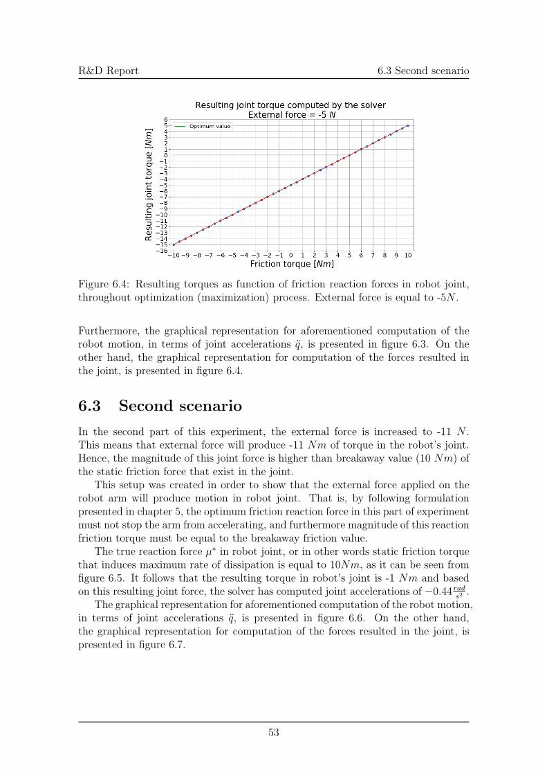
R&D Report 6.3 Second scenario

Figure 6.4: Resulting torques as function of friction reaction forces in robot joint,throughout optimization (maximization) process. External force is equal to -5N .

Furthermore, the graphical representation for aforementioned computation of therobot motion, in terms of joint accelerations q, is presented in figure 6.3. On theother hand, the graphical representation for computation of the forces resulted inthe joint, is presented in figure 6.4.

6.3 Second scenario

In the second part of this experiment, the external force is increased to -11 N .This means that external force will produce -11 Nm of torque in the robot’s joint.Hence, the magnitude of this joint force is higher than breakaway value (10 Nm) ofthe static friction force that exist in the joint.

This setup was created in order to show that the external force applied on therobot arm will produce motion in robot joint. That is, by following formulationpresented in chapter 5, the optimum friction reaction force in this part of experimentmust not stop the arm from accelerating, and furthermore magnitude of this reactionfriction torque must be equal to the breakaway friction value.

The true reaction force µ∗ in robot joint, or in other words static friction torquethat induces maximum rate of dissipation is equal to 10Nm, as it can be seen fromfigure 6.5. It follows that the resulting torque in robot’s joint is -1 Nm and basedon this resulting joint force, the solver has computed joint accelerations of −0.44 rad

s2.

The graphical representation for aforementioned computation of the robot motion,in terms of joint accelerations q, is presented in figure 6.6. On the other hand,the graphical representation for computation of the forces resulted in the joint, ispresented in figure 6.7.

53


Figure 6.5: Acceleration energy as function of friction reaction forces in robot joint.The reaction friction torque that induced maximum of acceleration energy is equalto 10 Nm.

Figure 6.6: Resulting accelerations as function of friction reaction forces in robotjoint, throughout optimization (maximization) process. External force is equal to-11N .

54


Figure 6.7: Resulting torques as function of friction reaction forces in robot joint,throughout optimization (maximization) process. External force is equal to -11N .

55

Chapter 7

Conclusion and future work

In this project, the extension for an already existing constrained hybrid dynamicssolver, namely Popov-Vereshchagin algorithm, has been presented. The approachfor including dissipative forces from static friction factors, in computations of energyoptimal instantaneous motions, has been completely derived.

The proof of concept evaluation in chapter 6 has shown the feasibility of theapproach proposed by Vereshchagin [4] and derived in this project. More specifically,the performed tests in a simulation environment with one DOF robot arm, haveshown that the approach for including static friction effects in computations ofmotions, provides correct results. Additionally, the experiments conducted usingthe extended algorithm, have shown that the Gauss function remains convex afterextension with friction forces. However, the function can take two forms dependingon a task (i.e. constraints) specified. That is, the cost function becomes linear ifa robot is fully constrained, else, if a robot is partially constrained then the Gaussfunction to be maximized takes quadratic form. This means that we require a genericmethod for maximizing the extended Gauss function (equation 5.9). In other words,we require an optimization technique that can be used for optimizing both linearand quadratic functions, depending on the constraints specified in run-time of arobot system.

The presented approach requires the use of the original Popov-Vereshchaginsolver, for computing the resulting motion and further on evaluating the Gaussfunction, for each set of the friction reaction forces considered throughout maximizationprocess. This procedure imposes a high computation load and may not be real-timefeasible. For that reason, the research in this project was conducted in order to derivethe (briefly outlined by Vereshchagin in [4]) method for improving the efficiency ofthe proposed extension to the original algorithm. More specifically, to reduce thenumber of operations (computations) required for finding the true reaction forcesand true motion of a system.

56

R&D Report

Aims of the future research in this field, involves the implementation of theconvex simplex method, in order to enable the use of the extended algorithm in thecomputation of motions, for the case of robot systems with an arbitrary number ofdegrees of freedom. This future plan includes investigation of the real-time feasibilityof the complete approach when the convex simplex method is implemented.Furthermore, future work would include implementation of the derived methodfor improving computational efficiency, which may remedy the issue of real-timeapplication of the complete approach.

Additionally, the future goal is to include dissipative forces induced by jointposition limits, in already derived general optimization procedure for additionalconditions, presented in section 5.2.

Finally, future work would concentrate on implementing the extended Popov-Vereshchagin algorithm on a real robot system. Furthermore, investigating additionalrequirements that may arise when the static friction effects are considered in computationsof energy optimal motions, in practical or in other words real robot environment.

57

Appendix A

Appendix

A.1 Plucker coordinates for spatial vectors

By using convention specified in terms of Plucker coordinates, we can define spatialvectors for both motions and forces. As Featherstone stated in [6], spatial vectors areconstructed by combining both angular and linear components of forces or motionsin a single vector. This type of 6D vector representation enables more efficientcomputation of rigid-body dynamic quantities, compared to traditional 3D vectorrepresentation [6].Generic representation of a spatial motion vector in Plucker coordinates is definedin the following form [6]:

M =

mL,x

mL,y

mL,z

mA,x

mA,y

mA,z

When spatial velocity and acceleration vectors are defined using this vector representation,they take following form:

X =

υxυyυzωx

ωy

ωz

, X =

υxυyυzωx

ωy

ωz

Here, symbols υ and ω represent linear and angular velocity components of a body,respectively. While symbols υ and ω represent linear and angular accelerationcomponents of a body, respectively.

58

R&D Report A.2 Coordinate transformation for motion and force vectors

On another side, representation of spatial force vector in Plucker coordinates isdefined in the following form [6]:

F =

fxfyfznx

ny

nz

Here, symbols f and n represent linear force and angular force (moment) componentsacting on a body, respectively.

A.2 Coordinate transformation for motion and force

vectors

Compared to general 4×4 homogeneous transformation matrix i+1i X [83], a coordinate

transformation 6×6 matrices for motion and force vectors are constructed differently.Namely, matrix i+1Xi (used for motion vectors) has be defined as [6]:

i+1Xi =

[E 0

−E r× E

](A.1)

where term E represents traditional 3 × 3 rotation matrix and term × denotes anoperators that maps a 3× 1 position vector r to a 3× 3 skew-symmetric matrix ofform:

r× =

x

y

z

× =

0 −z y

z 0 −x

−y x 0

(A.2)

Matrices for transformations of motion and force vectors are related in followingmanner: i+1X∗

i = i+1Xi−T

, and we can infer that i+1X∗

i is defined as:

i+1X∗

i =

[E −E r×0 E

](A.3)

59

R&D Report A.3 Cross product operators

A.3 Cross product operators

Cross product operators in Plucker coordinates X× and X×∗ represent 6×6 matriceswhich are defined as [6]:

X× =

[ω

υ

]× =

[ω× 0υ× ω×

](A.4)

X×∗ =

[ω

υ

]×∗ =

[ω× υ×0 ω×

]= −(X×)T (A.5)

where skew-symmetric matrices ω× and υ× are defined as:

ω× =

0 −ωz ωy

ωz 0 −ωx

−ωy ωx 0

(A.6)

υ× =

0 −υz υyυz 0 −υx−υy υx 0

(A.7)

60

References

[1] M. Brossog, M. Bornschlegl, J. Franke, et al., “Reducing the energy consumptionof industrial robots in manufacturing systems.”, International Journal of AdvancedManufacturing Technology, vol. 78, pp: 2346–2353, 2015.

[2] B. Bona and M. Indri, “Friction compensation in robotics: An overview”, inDecision and Control and European Control Conference IEEE, Seville, Spain,2005.

[3] C. Hansen, J. Oltjen, D. Meike, and T. Ortmaier, “Enhanced approach forenergy-efficient trajectory generation of industrial robots”, in IEEE InternationalConference on Automation Science and Engineering, 2012.

[4] A. F. Vereshchagin, “Modelling and control of motion of manipulation robots”,Soviet Journal of Computer and Systems Sciences, vol. 27, pp. 29–38, 1989.

[5] E. P. Popov, A. F. Vereshchagin, and S. L. Zenkevich, “Manipulyatsionnyeroboty: Dinamika i algoritmy”, Nauka, Moscow, 1978.

[6] R. Featherstone, Rigid body dynamics algorithms. Springer, 2008.

[7] R. Featherstone, “Robot dynamics”, Scholarpedia, vol. 2, p. 3829, 2007.

[8] A. Shakhimardanov, “Composable robot motion stack: Implementing constrainedhybrid dynamics using semantic models of kinematic chains”, PhD thesis, KULeuven, 2015.

[9] M. L. Felis, “RBDL: an efficient rigid-body dynamics library using recursivealgorithms”, Autonomous Robots, vol. 41, pp. 495–511, 2017.

[10] P. Lotstedt, “Mechanical systems of rigid bodies subject to unilateral constraints”,SIAM Journal on Applied Mathematics, vol. 42, pp. 281–296, 1982.

[11] S. Ivaldi, V. Padois, and F. Nori, “Tools for dynamics simulation of robots:A survey based on user feedback”, IEEE-RAS International Conference onHumanoid Robots (Humanoids), 2014.

[12] E. Todorov, T. Erez, and Y. Tassa, “Mujoco: A physics engine for model-based control”, in IEEE/RSJ International Conference on Intelligent Robotsand Systems (IROS), 2012.

[13] R. Smith, ODE physics engine, Accessed 2017-05-21, [Online] Available: http://ode.org/.

[14] Georgia, Institute of Technology, DART physics engine, Accessed: 2017-05-21,[Online] Available: http://dartsim.github.io/.

61

http://ode.org/

http://ode.org/

http://dartsim.github.io/

R&D Report REFERENCES

[15] Erwin Coumans, Bullet physics engine, Accessed: 2017-05-21, [Online] Available:http://bulletphysics.org/.

[16] M. A. Sherman, A. Seth, and S. L. Delp, “Simbody: Multibody dynamics forbiomedical research”, Procedia Iutam, vol. 2, pp. 241–261, 2011.

[17] R. Smits, E. Aertbelien, H. Bruyninckx, and A. Shakhimardanov, Kinematicsand Dynamics Library (KDL), Accessed: 2017-05-30, [Online] Available: http://www.orocos.org/kdl.

[18] M. Quigley, K. Conley, B. Gerkey, J. Faust, T. Foote, J. Leibs, R. Wheeler,and A. Y. Ng, “ROS: an open-source Robot Operating System”, in ICRAworkshop on open source software, 2009.

[19] N. Mansard and F. Valenza, Pinocchio library, Accessed: 2017-07-25, [Online]Available: https://stack-of-tasks.github.io/pinocchio/.

[20] Joint Japanese French Robotics Lab, JRL-RBDyn library, Accessed: 2017-07-25, [Online] Available: https://jrl-umi3218.github.io/RBDyn/doxygen/HEAD/index.html.

[21] B. Armstrong-Helouvry, P. Dupont, and C. C. De Wit, “A survey of models,analysis tools and compensation methods for the control of machines withfriction”, Automatica, vol. 30, 1994.

[22] J. Moreno, R. Kelly, and R. Campa, “On manipulator velocity control usingfriction compensation”, in IEEE International Conference on Robotics andAutomation, 2002.

[23] A. A. Ata, “Optimal trajectory planning of manipulators: A review”, Journalof Engineering Science and Technology, vol. 2, pp. 32–54, 2007.

[24] S.-H. Lee, J. Kim, F. C. Park, M. Kim, and J. E. Bobrow, “Newton-typealgorithms for dynamics-based robot movement optimization”, IEEE Transactionson Robotics, vol. 21, pp. 657–667, 2005.

[25] J. Kim, J. Baek, and F. C. Park, “Newton-type algorithms for robot motionoptimization”, in International Conference on Intelligent Robots and Systems,1999.

[26] B. J. Martin and J. E. Bobrow, “Minimum-effort motions for open-chainmanipulators with task-dependent end-effector constraints”, The InternationalJournal of Robotics Research, vol. 18, pp. 213–224, 1999.

[27] D. Verscheure, B. Demeulenaere, J. Swevers, J. D. Schutter, and M. Diehl,“Time-energy optimal path tracking for robots: A numerically efficient optimizationapproach”, in IEEE International Workshop on Advanced Motion Control,2008.

[28] G. S. Sharma, M. Singh, and T. Singh, “Optimization of energy in roboticarm using genetic algorithm”, International Journal of Computer Science andTechnology, vol. 2, pp. 315–317, 2011.

[29] D. P. Garg and M. Kumar, “Optimization techniques applied to multiplemanipulators for path planning and torque minimization”, Engineering Applicationsof Artificial Intelligence, vol. 15, pp. 241 –252, 2002.

62

http://bulletphysics.org/

http://www.orocos.org/kdl

http://www.orocos.org/kdl

https://stack-of-tasks.github.io/pinocchio/

https://jrl-umi3218.github.io/RBDyn/doxygen/HEAD/index.html

https://jrl-umi3218.github.io/RBDyn/doxygen/HEAD/index.html


[30] H. Bruyninckx and O. Khatib, “Gauss’ principle and the dynamics of redundantand constrained manipulators”, in IEEE International Conference on Roboticsand Automation, 2000.

[31] O. Khatib, L. Sentis, J. Park, and J. Warren, “Whole-body dynamic behaviorand control of human-like robots”, International Journal of Humanoid Robotics,vol. 1, 2004.

[32] O. Khatib, “A unified approach for motion and force control of robot manipulators:The operational space formulation”, IEEE Journal on Robotics and Automation,vol. 3, pp. 43–53, 1987.

[33] N. Mansard, O. Khatib, and A. Kheddar, “A unified approach to integrateunilateral constraints in the stack of tasks”, IEEE Transactions on Robotics,vol. 25, 2009.

[34] R. Smits, T. De Laet, K. Claes, H. Bruyninckx, and J. De Schutter, “iTaSC: ATool for Multi-Sensor Integration in Robot Manipulation”, in IEEE InternationalConference on Multisensor Fusion and Integration for Intelligent Systems 2008.

[35] K.-S. Chang and O. Khatib, “Operational space dynamics: Efficient algorithmsfor modeling and control of branching mechanisms”, in IEEE InternationalConference on Robotics and Automation., 2000.

[36] L. Sentis and O. Khatib, “A whole-body control framework for humanoidsoperating in human environments”, in Robotics and Automation, IEEE InternationalConference on, 2006.

[37] O. Khatib and L. Sentis, “Synthesis of whole-body behaviors through hierarchicalcontrol of behavioral primitives”, International Journal of Humanoid Robotics,vol. 2, pp. 505–518, 2005.

[38] O. Khatib, L. Sentis, and J.-H. Park, “A unified framework for whole-bodyhumanoid robot control with multiple constraints and contacts”, in EuropeanRobotics Symposium 2008, pp. 303–312.

[39] J. Nakanishi, R. Cory, M. Mistry, J. Peters, and S. Schaal, “Operational spacecontrol: A theoretical and empirical comparison”, The International Journalof Robotics Research, vol. 27, pp. 737–757, 2008.

[40] R. M. Murray, Z. Li, S. S. Sastry, and S. S. Sastry, A mathematical introductionto robotic manipulation. CRC press, 1994.

[41] C.-L. Fok, G. Johnson, J. D. Yamokoski, A. Mok, and L. Sentis, “Controlit! asoftware framework for whole-body operational space control”, InternationalJournal of Humanoid Robotics, vol. 13, 2016.

[42] M. Felis, Rigid body dynamics library (RBDL), Accessed: 2017-06-20, [Online]Available: https://rbdl.bitbucket.io/.

[43] F Furrer, M Burri, M Achtelik, and R Siegwart, “Robot Operating System(ROS): The Complete Reference (Volume 1)”, By A. Koubaa. Cham: SpringerInternational Publishing, 2016.

63

https://rbdl.bitbucket.io/


[44] D. Vanthienen, T. De Laet, W. Decre, R. Smits, M. Klotzbucher, K. Buys, S.Bellens, L. Gherardi, H. Bruyninckx, and J. De Schutter, “iTaSC as a unifiedframework for task specification, control, and coordination, demonstrated onthe PR2”, in IEEE International Conference on Mechatronics and Robotics,2011.

[45] I. A. Sucan and S. Chitta, MoveIt!, Accessed: 2017-06-18, [Online] Available:http://moveit.ros.org.

[46] N. Mansard, O. Stasse, P. Evrard, and A. Kheddar, “A versatile generalizedinverted kinematics implementation for collaborative working humanoid robots:The stack of tasks”, in International Conference on Advanced Robotics, 2009.

[47] L. Saab, N. Mansard, F. Keith, J. Y. Fourquet, and P. Soueres, “Generation ofdynamic motion for anthropomorphic systems under prioritized equality andinequality constraints”, in IEEE International Conference on Robotics andAutomation, 2011.

[48] L. Saab, O. Ramos, N. Mansard, P. Soures, and J. Y. Fourquet, “Genericdynamic motion generation with multiple unilateral constraints”, in IEEE/RSJInternational Conference on Intelligent Robots and Systems, 2011.

[49] N. Mansard, “A dedicated solver for fast operational-space inverse dynamics”,in IEEE International Conference on Robotics and Automation, 2012.

[50] L. Saab, O. E. Ramos, F. Keith, N. Mansard, P. Soueres, and J.-Y. Fourquet,“Dynamic whole-body motion generation under rigid contacts and other unilateralconstraints”, IEEE Transactions on Robotics, vol. 29, 2013.

[51] A. Escande, N. Mansard, and P.-B. Wieber, “Hierarchical quadratic programming:Fast online humanoid-robot motion generation”, The International Journal ofRobotics Research, vol. 33, 2014.

[52] Lamiraux, Florent and Stasse, Olivier and Mansard, Nicolas, Stack of Tasks,Accessed: 2017-05-30, [Online] Available: http://stack-of-tasks.github.io/.

[53] Y. Nakamura and H. Hanafusa, “Optimal redundancy control of robot manipulators”,The International Journal of Robotics Research, vol. 6, pp. 32–42, 1987.

[54] S. B. Slotine, “A general framework for managing multiple tasks in highlyredundant robotic systems”, in proceeding of 5th International Conference onAdvanced Robotics, 1991.

[55] R. Fletcher, “A general quadratic programming algorithm”, IMA Journal ofApplied Mathematics, vol. 7, pp. 76–91, 1971.

[56] J. De Schutter, T. De Laet, J. Rutgeerts, W. Decre, R. Smits, E. Aertbelien, K.Claes, and H. Bruyninckx, “Constraint-based task specification and estimationfor sensor-based robot systems in the presence of geometric uncertainty”, TheInternational Journal of Robotics Research, vol. 26, pp. 433–455, 2007.

[57] W. Decre, R. Smits, H. Bruyninckx, and J. D. Schutter, “Extending itasc tosupport inequality constraints and non-instantaneous task specification”, in2009 IEEE International Conference on Robotics and Automation.

64

http://moveit.ros.org

http://stack-of-tasks.github.io/

http://stack-of-tasks.github.io/


[58] W. Decr, H. Bruyninckx, and J. D. Schutter, “Extending the itasc constraint-based robot task specification framework to time-independent trajectoriesand user-configurable task horizons”, in IEEE International Conference onRobotics and Automation, 2013.

[59] R. Smits, H. Bruyninckx, and J. D. Schutter, “iTaSC (instantaneous TaskSpecification using Constraints)”, Accessed: 2017-09-27, [Online] Available:http://www.orocos.org/wiki/orocos/itasc-wiki.

[60] A. F. Vereshchagin, “Computer simulation of the dynamics of complicatedmechanisms of robot-manipulators”, Engineering Cybernetics, 12(6), pp. 65–70, 1974.

[61] E. P. Popov, “Control of robots-manipulators”, Engineering Cybernetics, 1974.

[62] C. F. Gauß, “Uber ein neues allgemeines Grundgesetz der Mechanik.”, Journalfur die reine und angewandte Mathematik, vol. 4, pp. 232–235, 1829.

[63] E. Ramm, “Principles of least action and of least constraint”,GAMM-Mitteilungen,vol. 34, pp. 164–182, 2011.

[64] J. L. Lagrange, “Mecanique analytique”, Mallet-Bachelier, vol. 1, 1853.

[65] R. Bellman, “On the theory of dynamic programming”, Proceedings of theNational Academy of Sciences, vol. 38, pp. 716–719, 1952.

[66] K. Yunt, “On the relation of the principle of maximum dissipation to theprinciples of jourdain and gauss for rigid body systems”, Journal of Computationaland Nonlinear Dynamics, vol. 9, p. 031 017, 2014.

[67] F. E. Udwadia and R. E. Kalaba, “A new perspective on constrained motion”,Proceedings: Mathematical and Physical Sciences, pp. 407–410, 1992.

[68] K. M. Lynch and F. C. Park, Modern Robotics: Mechanics, Planning, andControl. Cambridge University Press, 2017.

[69] A. Albu-Schaffer and G. Hirzinger, “Cartesian impedance control techniquesfor torque controlled light-weight robots”, in IEEE International Conferenceon Robotics and Automation, 2002.

[70] B. Siciliano and O. Khatib, Springer handbook of robotics. Springer, 2016.

[71] J. De Schutter, D. Torfs, H. Bruyninckx, and S. Dutre, “Invariant hybridforce/position control of a velocity controlled robot with compliant end effectorusing modal decoupling”, The International Journal of Robotics Research,vol. 16, pp. 340–356, 1997.

[72] E. Berger, “Friction modeling for dynamic system simulation”, Applied MechanicsReviews, vol. 55, pp. 535–577, 2002.

[73] J. S. Eck and W. Thompson, “Dissipative forces and quantum mechanics”,American Journal of Physics, vol. 45, pp. 161–163, 1977.

[74] D. E. Stewart, “Rigid-body dynamics with friction and impact”, SIAM review,vol. 42, pp. 3–39, 2000.

65

http://www.orocos.org/wiki/orocos/itasc-wiki


[75] E. Drumwright and D. A. Shell, “Modeling contact friction and joint frictionin dynamic robotic simulation using the principle of maximum dissipation”,Algorithmic foundations of robotics IX, pp. 249–266, 2010.

[76] G. Pozharitskii, “Extension of the principle of gauss to systems with dry(coulomb) friction”, Journal of Applied Mathematics and Mechanics, vol. 25,pp. 586 –607, 1961.

[77] H. Olsson, M. Gafvert, and P. Lischinsky, “Friction models and friction compensation”,European Journal of Control, vol. 4, pp. 176–195, 1998.

[78] S. Boyd and L. Vandenberghe, Convex optimization. Cambridge universitypress, 2004.

[79] F. Alizadeh, “Interior point methods in semidefinite programming with applicationsto combinatorial optimization”, SIAM journal on Optimization, vol. 5, pp. 13–51, 1995.

[80] W. I. Zangwill, “The convex simplex method”, Management Science, vol. 14,pp. 221–238, 1967.

[81] A. D. Polyanin, W. E. Schiesser, and A. I. Zhurov, “Partial differential equation”,Scholarpedia, vol. 3, 2008.

[82] A. Brondsted, An introduction to convex polytopes. Springer Science & BusinessMedia, vol. 90, 2012.

[83] J. J. Craig, Introduction to robotics: mechanics and control. Pearson PrenticeHall Upper Saddle River, vol. 3, 2005.

66

extending a constrained hybrid dynamics solver for energy

Documents