explosion in branching processes and applications to ... · explosion in branching processes and...
TRANSCRIPT

Explosion in branching processes and applications toepidemics in random graph models
Julia Komjathy
joint with Enrico Baroni and Remco van der HofstadEindhoven University of Technology
Advances on Epidemics in Complex Networks31 Aug 2017
Julia Komjathy (TU/e) 1 / 44

Class of processes on networks
Spreading processes
Includes
Julia Komjathy (TU/e) 2 / 44

Class of processes on networks
Information diffusion
Includes
Julia Komjathy (TU/e) 2 / 44

Class of processes on networks
Includes
Julia Komjathy (TU/e) 2 / 44

Viruses
Julia Komjathy (TU/e) 3 / 44

Viruses
The spread of the west-nile-virus
Julia Komjathy (TU/e) 4 / 44

Viruses
The spread of the Zika virus
Julia Komjathy (TU/e) 5 / 44

Memes
Julia Komjathy (TU/e) 6 / 44

Memes
Julia Komjathy (TU/e) 7 / 44

Viral videos
Julia Komjathy (TU/e) 8 / 44

Extremely fast spread
Search intensity of Gangnam style
from knowyourmeme.com
Julia Komjathy (TU/e) 9 / 44

Extremely fast spread
Search intensity of the Slenderman meme
from knowyourmeme.com
Julia Komjathy (TU/e) 10 / 44

Extremely fast spread
Epidemic curve of a flu from China
from Center for Infectious Disease Research and Policy
Julia Komjathy (TU/e) 11 / 44

Modeling
We need models!
Julia Komjathy (TU/e) 12 / 44

The scale-free property
Many real-life networks have power-law degrees.
Power-law paradigm
For some τ > 2, the degree of a uniformly chosen vertex satisfies
P(deg(v) = x) � C
xτ
logP(deg(v) = x) � logC − τ log x
log(proportion of degree x vertices) vs log x is a straight line.
Julia Komjathy (TU/e) 13 / 44

Power laws
Degree distribution of the router level internet networkfrom Faloutsos, Faloutsos, Faloutsos. 1999
Julia Komjathy (TU/e) 14 / 44

Power laws
Degree distribution of ecological networksfrom Montoya, Pimm, Pole. Nature 2006
Julia Komjathy (TU/e) 15 / 44

Power laws
Note: τ ∈ (2, 3) often!
When τ ∈ (2, 3) then Varn[deg(v)]→∞ and En[deg(v)] <∞.
Julia Komjathy (TU/e) 16 / 44

Choice of model
Configuration model
Julia Komjathy (TU/e) 17 / 44

The configuration model
Matches the degree sequence of the network you would like to model.
[Configuration model simulator by Robert Fitzner]
[Configuration model with power law degrees by Robert Fitzner]
Power-law assumption
For some τ ∈ (2, 3), the tail of the empirical degree distribution satisfies
c1
xτ−1≤ [1− Fn](x) = P(deg(vn) ≥ x) ≤ C1
xτ−1
Julia Komjathy (TU/e) 18 / 44

Weighted Configuration model
Information diffusion
Transmission times through edges are random in real networks.Modeling: each edge has an independent weight from the samedistribution σ.
Independence might not hold in real-life, but makes the analysis tractable.
Spreading time = weighted distance
The spreading time between two vertices u, v= the weighted distance:
dσ(u, v)
How does dσ(u, v) behave in terms of the degrees and the edge-weightdistribution σ?
Julia Komjathy (TU/e) 19 / 44

Weighted Configuration model
Information diffusion
Transmission times through edges are random in real networks.Modeling: each edge has an independent weight from the samedistribution σ.Independence might not hold in real-life, but makes the analysis tractable.
Spreading time = weighted distance
The spreading time between two vertices u, v= the weighted distance:
dσ(u, v)
How does dσ(u, v) behave in terms of the degrees and the edge-weightdistribution σ?
Julia Komjathy (TU/e) 19 / 44

The epidemic curve
Epidemic curve
Considering vertex u as a (single) source of infection, σe as thetransmission time of an infection through edge e, the epidemic curve isdefined as
Iu(t) =1
|V |∑v∈V
1dσ(u,v)≤t .
How does Iu(t) behave, in terms of the degree distribution, theedge-length distribution σ, and the source vertex u?
Julia Komjathy (TU/e) 20 / 44
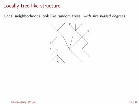
Locally tree-like structure
Local neighborhoods look like random trees with size biased degrees.
Size-biasing effect
A neighbor of a uniform vertex is more likely to have larger degree
P(
deg(neighbor(v)) > x)� Cx
xτ−1=
C
xτ−2
Julia Komjathy (TU/e) 21 / 44

Locally tree-like structure
Local neighborhoods look like random trees with size biased degrees.
Size-biasing effect
A neighbor of a uniform vertex is more likely to have larger degree
P(
deg(neighbor(v)) > x)� Cx
xτ−1=
C
xτ−2
Julia Komjathy (TU/e) 21 / 44

Preliminaries
Initial stage of the spreading in the graph looks like a random tree with
power law degrees, tail exponent α := τ − 2 ∈ (0, 1)
each edge has an independent ‘length’ or ‘weight’
Julia Komjathy (TU/e) 22 / 44

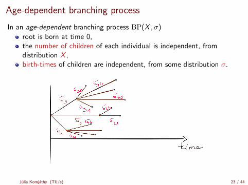
Age-dependent branching process
In an age-dependent branching process BP(X , σ)
root is born at time 0,
the number of children of each individual is independent, fromdistribution X ,
birth-times of children are independent, from some distribution σ.
Julia Komjathy (TU/e) 23 / 44

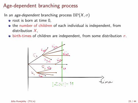
Age-dependent branching process
In an age-dependent branching process BP(X , σ)
root is born at time 0,
the number of children of each individual is independent, fromdistribution X ,birth-times of children are independent, from some distribution σ.
Julia Komjathy (TU/e) 23 / 44

Age-dependent branching process
In an age-dependent branching process BP(X , σ)
root is born at time 0,the number of children of each individual is independent, fromdistribution X ,
birth-times of children are independent, from some distribution σ.
Julia Komjathy (TU/e) 23 / 44
Age-dependent branching process
In an age-dependent branching process BP(X , σ)
root is born at time 0,the number of children of each individual is independent, fromdistribution X ,birth-times of children are independent, from some distribution σ.
Julia Komjathy (TU/e) 23 / 44
Age-dependent branching process
In an age-dependent branching process BP(X , σ)
root is born at time 0,the number of children of each individual is independent, fromdistribution X ,birth-times of children are independent, from some distribution σ.
Julia Komjathy (TU/e) 23 / 44
Explosion?
Definition
D(t) = population born by time t.
A branching process is explosive if for some t > 0,
P(|D(t)| =∞) > 0.
Otherwise conservative.
Explosive vs conservative
When is a branching process BP(X , σ) explosive?
Julia Komjathy (TU/e) 24 / 44

Explosion?
Definition
D(t) = population born by time t.A branching process is explosive if for some t > 0,
P(|D(t)| =∞) > 0.
Otherwise conservative.
Explosive vs conservative
When is a branching process BP(X , σ) explosive?
Julia Komjathy (TU/e) 24 / 44

Explosion?
Definition
D(t) = population born by time t.A branching process is explosive if for some t > 0,
P(|D(t)| =∞) > 0.
Otherwise conservative.
Explosive vs conservative
When is a branching process BP(X , σ) explosive?
Julia Komjathy (TU/e) 24 / 44

Explosion?
Definition
D(t) = population born by time t.A branching process is explosive if for some t > 0,
P(|D(t)| =∞) > 0.
Otherwise conservative.
Explosive vs conservative
When is a branching process BP(X , σ) explosive?
Julia Komjathy (TU/e) 24 / 44
Explosion of BPs
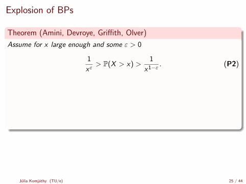
Theorem (Amini, Devroye, Griffith, Olver)
Assume for x large enough and some ε > 0
1
xε> P(X > x) >
1
x1−ε . (P2)
The branching process BP(X , σ) is explosive if and only if for some K > 0
∞∑K
F (−1)σ
(e−e
k)<∞ (I)
where F(−1)σ is the generalised inverse of the distribution function of σ.
Corollary
If a distribution σ satisfies (I) then it explodes for all X satisfying (P2)(including all power law degrees with τ ∈ (2, 3)).
Julia Komjathy (TU/e) 25 / 44

Explosion of BPs
Theorem (Amini, Devroye, Griffith, Olver)
Assume for x large enough and some ε > 0
1
xε> P(X > x) >
1
x1−ε . (P2)
The branching process BP(X , σ) is explosive if and only if for some K > 0
∞∑K
F (−1)σ
(e−e
k)<∞ (I)
where F(−1)σ is the generalised inverse of the distribution function of σ.
Corollary
If a distribution σ satisfies (I) then it explodes for all X satisfying (P2)(including all power law degrees with τ ∈ (2, 3)).
Julia Komjathy (TU/e) 25 / 44

Explosive σ-s
∑k≥K F
(−1)σ
(e−e
k)<∞ is easy to check.
Examples
Flatness of distribution function Fσ at the origin matters.
Exponential, Gamma, Uniform, etc.
Fσ(t) = exp{−1/tβ}, β > 0
Boundary case: Fσ(t) = exp{− exp{ 1tβ}}. Explosive for β < 1,
conservative for β ≥ 1.
Fσ does not have to be continuous to satisfy (I): e.g. put point-massck1 /(1− c) to points at ck2 , for c1, c2 < 1.
Julia Komjathy (TU/e) 26 / 44

Application to epidemics in random graphs
Julia Komjathy (TU/e) 27 / 44

Explosive weights on the configuration model
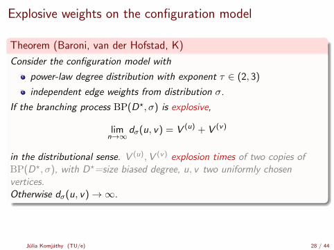
Theorem (Baroni, van der Hofstad, K)
Consider the configuration model with
power-law degree distribution with exponent τ ∈ (2, 3)
independent edge weights from distribution σ.
If the branching process BP(D?, σ) is explosive,
limn→∞
dσ(u, v) = V (u) + V (v)
in the distributional sense. V (u),V (v) explosion times of two copies ofBP(D?, σ), with D?=size biased degree, u, v two uniformly chosenvertices.Otherwise dσ(u, v)→∞.
This was first shown for exponential edge weights by Bhamidi, Hofstad &Hooghiemstra.
Julia Komjathy (TU/e) 28 / 44

Explosive weights on the configuration model
Theorem (Baroni, van der Hofstad, K)
Consider the configuration model with
power-law degree distribution with exponent τ ∈ (2, 3)
independent edge weights from distribution σ.
If the branching process BP(D?, σ) is explosive,
limn→∞
dσ(u, v) = V (u) + V (v)
in the distributional sense. V (u),V (v) explosion times of two copies ofBP(D?, σ), with D?=size biased degree, u, v two uniformly chosenvertices.
Otherwise dσ(u, v)→∞.
This was first shown for exponential edge weights by Bhamidi, Hofstad &Hooghiemstra.
Julia Komjathy (TU/e) 28 / 44
Explosive weights on the configuration model
Theorem (Baroni, van der Hofstad, K)
Consider the configuration model with
power-law degree distribution with exponent τ ∈ (2, 3)
independent edge weights from distribution σ.
If the branching process BP(D?, σ) is explosive,
limn→∞
dσ(u, v) = V (u) + V (v)
in the distributional sense. V (u),V (v) explosion times of two copies ofBP(D?, σ), with D?=size biased degree, u, v two uniformly chosenvertices.Otherwise dσ(u, v)→∞.
This was first shown for exponential edge weights by Bhamidi, Hofstad &Hooghiemstra.
Julia Komjathy (TU/e) 28 / 44

Explosive weights on the configuration model
Theorem (Baroni, van der Hofstad, K)
Consider the configuration model with
power-law degree distribution with exponent τ ∈ (2, 3)
independent edge weights from distribution σ.
If the branching process BP(D?, σ) is explosive,
limn→∞
dσ(u, v) = V (u) + V (v)
in the distributional sense. V (u),V (v) explosion times of two copies ofBP(D?, σ), with D?=size biased degree, u, v two uniformly chosenvertices.Otherwise dσ(u, v)→∞.
This was first shown for exponential edge weights by Bhamidi, Hofstad &Hooghiemstra.
Julia Komjathy (TU/e) 28 / 44

Corrollary: Epidemic curve in the explosive case
Recall Iu(t) = 1|V |∑
v∈V 1dσ(u,v)≤t is the epidemic curve.
Convergence of the epidemic curve
Consider an epidemic started at a single, uniformly chosen vertex u ∈ V .Then
Iu(t)P−→ f (t − V (u)) = P(V (u) + V (v) ≤ t | V (u))
A deterministic curve with a random but constant shift V (u).
Julia Komjathy (TU/e) 29 / 44

Conservative weights on the configuration model
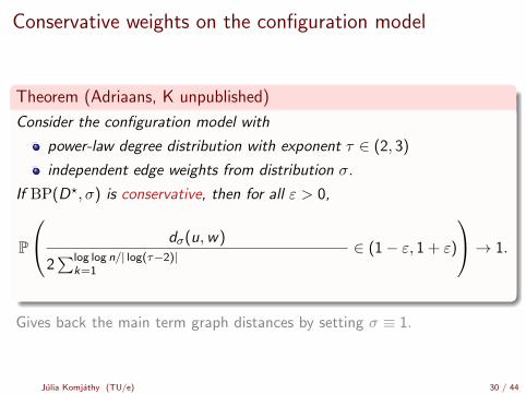
Theorem (Adriaans, K unpublished)
Consider the configuration model with
power-law degree distribution with exponent τ ∈ (2, 3)
independent edge weights from distribution σ.
If BP(D?, σ) is conservative, then for all ε > 0,
P
dσ(u,w)
2∑log log n/| log(τ−2)|
k=1 F(−1)σ
(exp
(− ( 1
τ−2 )k))
∈ (1− ε, 1 + ε)
→ 1.
Gives back the main term graph distances by setting σ ≡ 1.
Julia Komjathy (TU/e) 30 / 44

Conservative weights on the configuration model
Theorem (Adriaans, K unpublished)
Consider the configuration model with
power-law degree distribution with exponent τ ∈ (2, 3)
independent edge weights from distribution σ.
If BP(D?, σ) is conservative, then for all ε > 0,
P
dσ(u,w)
2∑log log n/| log(τ−2)|
k=1 F(−1)σ
(exp
(− ( 1
τ−2 )k))
∈ (1− ε, 1 + ε)
→ 1.
Gives back the main term graph distances by setting σ ≡ 1.
Julia Komjathy (TU/e) 30 / 44
Conservative weights on the configuration model
Theorem (Adriaans, K unpublished)
Consider the configuration model with
power-law degree distribution with exponent τ ∈ (2, 3)
independent edge weights from distribution σ.
If BP(D?, σ) is conservative, then for all ε > 0,
P
dσ(u,w)
2∑log log n/| log(τ−2)|
k=1
F(−1)σ
(exp
(− ( 1
τ−2 )k))
∈ (1− ε, 1 + ε)
→ 1.
Gives back the main term graph distances by setting σ ≡ 1.
Julia Komjathy (TU/e) 30 / 44

Conservative weights on the configuration model
Theorem (Adriaans, K unpublished)
Consider the configuration model with
power-law degree distribution with exponent τ ∈ (2, 3)
independent edge weights from distribution σ.
If BP(D?, σ) is conservative, then for all ε > 0,
P
dσ(u,w)
2∑log log n/| log(τ−2)|
k=1 F(−1)σ
(exp
(− ( 1
τ−2 )k)) ∈ (1− ε, 1 + ε)
→ 1.
Gives back the main term graph distances by setting σ ≡ 1.
Julia Komjathy (TU/e) 30 / 44

Not enough...
For an epidemic curve one would need distributional convergence of thefluctuations of dσ(u, v) around
2∑log log n/| log(τ−2)|
k=1 F(−1)σ
(exp
(− ( 1
τ−2 )k))
which is not known/not
possible to show with our current methods.
Julia Komjathy (TU/e) 31 / 44
When τ > 3
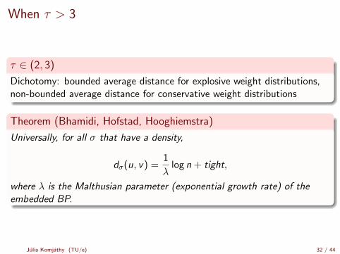
τ ∈ (2, 3)
Dichotomy: bounded average distance for explosive weight distributions,non-bounded average distance for conservative weight distributions
Theorem (Bhamidi, Hofstad, Hooghiemstra)
Universally, for all σ that have a density,
dσ(u, v) =1
λlog n + tight,
where λ is the Malthusian parameter (exponential growth rate) of theembedded BP.
Julia Komjathy (TU/e) 32 / 44
Generalisation to spatial models
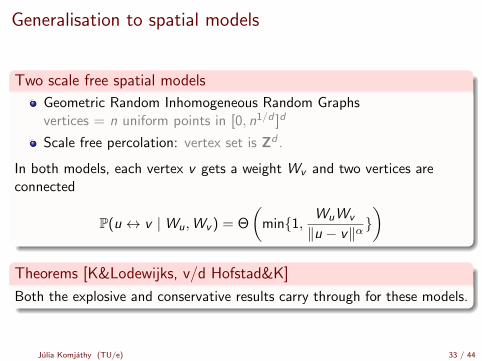
Two scale free spatial models
Geometric Random Inhomogeneous Random Graphsvertices = n uniform points in [0, n1/d ]d
Scale free percolation: vertex set is Zd .
In both models, each vertex v gets a weight Wv and two vertices areconnected
P(u ↔ v |Wu,Wv ) = Θ
(min{1, WuWv
‖u − v‖α})
Theorems [K&Lodewijks, v/d Hofstad&K]
Both the explosive and conservative results carry through for these models.
Julia Komjathy (TU/e) 33 / 44

Epidemics with contagious intervals
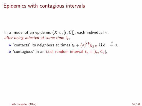
In a model of an epidemic (X , σ, [I ,C ]), each individual v ,after being infected at some time tv ,
‘contacts’ its neighbors at times tv + (σ(v)i )i≤X i.i.d.
d= σ,
‘contagious’ in an i.i.d. random interval tv + [Iv ,Cv ],
only those friends will be infected that satisfy σ(v)i ∈ [Iv ,Cv ].
Julia Komjathy (TU/e) 34 / 44

Epidemics with contagious intervals
In a model of an epidemic (X , σ, [I ,C ]), each individual v ,after being infected at some time tv ,
‘contacts’ its neighbors at times tv + (σ(v)i )i≤X i.i.d.
d= σ,
‘contagious’ in an i.i.d. random interval tv + [Iv ,Cv ],
only those friends will be infected that satisfy σ(v)i ∈ [Iv ,Cv ].
Julia Komjathy (TU/e) 34 / 44

Explosion in this case?
Epidemics with contagious intervals
When is a triplet (X , σ, [I ,C ]) explosive?Can the explosion of BP(X , σ) be stopped by adding [I ,C ] to it?
Julia Komjathy (TU/e) 35 / 44

Getting rid of end of interval
Heuristics: Explosion is carried by short edges, so deleting long edges doesnot matter.
Theorem (K)
Suppose X satisfies (P2) and [I ,C ] satisfies ∃t0, δ > 0
P(C > t|I = i) ≥ δ ∀i < t < t0. (?)
Then (X , σ, [I ,C ]) explosive ⇔ (X , σ, [I ,∞]) explosive.
Natural condition
Condition (?) on [I ,C ] is satisfied if
I ,C independent, C 6≡ 0.
C = I + L with I , L independent, L 6≡ 0.
It means that the support of I , L is not concentrated on a ‘slentedwedge’ separating the support from the L axes.
Julia Komjathy (TU/e) 36 / 44

Explosion of epidemics with incubation time
Heuristics: Explosion is carried by short edges, so deleting short edges doesmatter.
Theorem (K)
Suppose X satisfies (P2), thenBP(X , σ, [I ,∞]) explosive ⇔ BP(X , σ),BP(X , I ) both explosive.
Coupling argument: If (X , I ) does not explode, all its rays haveinfinite length
in (X , σ, [I ,∞]) only edges with σv > Iv are kept,and (X , I ) is conservativeso (X , σ, [I ,∞]) does not explode either.
Other way round trickier...
Julia Komjathy (TU/e) 37 / 44

Explosion of epidemics with incubation time
Heuristics: Explosion is carried by short edges, so deleting short edges doesmatter.
Theorem (K)
Suppose X satisfies (P2), thenBP(X , σ, [I ,∞]) explosive ⇔ BP(X , σ),BP(X , I ) both explosive.
Coupling argument: If (X , I ) does not explode, all its rays haveinfinite lengthin (X , σ, [I ,∞]) only edges with σv > Iv are kept,
and (X , I ) is conservativeso (X , σ, [I ,∞]) does not explode either.
Other way round trickier...
Julia Komjathy (TU/e) 37 / 44

Explosion of epidemics with incubation time
Heuristics: Explosion is carried by short edges, so deleting short edges doesmatter.
Theorem (K)
Suppose X satisfies (P2), thenBP(X , σ, [I ,∞]) explosive ⇔ BP(X , σ),BP(X , I ) both explosive.
Coupling argument: If (X , I ) does not explode, all its rays haveinfinite lengthin (X , σ, [I ,∞]) only edges with σv > Iv are kept,and (X , I ) is conservative
so (X , σ, [I ,∞]) does not explode either.
Other way round trickier...
Julia Komjathy (TU/e) 37 / 44

Explosion of epidemics with incubation time
Heuristics: Explosion is carried by short edges, so deleting short edges doesmatter.
Theorem (K)
Suppose X satisfies (P2), thenBP(X , σ, [I ,∞]) explosive ⇔ BP(X , σ),BP(X , I ) both explosive.
Coupling argument: If (X , I ) does not explode, all its rays haveinfinite lengthin (X , σ, [I ,∞]) only edges with σv > Iv are kept,and (X , I ) is conservativeso (X , σ, [I ,∞]) does not explode either.
Other way round trickier...
Julia Komjathy (TU/e) 37 / 44
Epidemics on the configuration model
Theorem (K, unpublished)
Consider the epidemic model on the configuration model with
power-law degrees with τ ∈ (2, 3)
i.i.d. contact times on edgesd= σ
i.i.d. contagious intervals on verticesd= [I ,C ].
u, v chosen uniformly at random
Julia Komjathy (TU/e) 38 / 44

Epidemics on the configuration model
Theorem (K, unpublished)
Consider the epidemic model on the configuration model with
power-law degrees with τ ∈ (2, 3)
i.i.d. contact times on edgesd= σ
i.i.d. contagious intervals on verticesd= [I ,C ].
u, v chosen uniformly at random
For the infection started from u, the time it takes to infect v :
depi(u, v)d−→ V (u) + V
(v)bw
if and only if (D?, σ, [I ,C ]) is explosive,
Julia Komjathy (TU/e) 38 / 44

Epidemics on the configuration model
Theorem (K, unpublished)
Consider the epidemic model on the configuration model with
power-law degrees with τ ∈ (2, 3)
i.i.d. contact times on edgesd= σ
i.i.d. contagious intervals on verticesd= [I ,C ].
u, v chosen uniformly at random
For the infection started from u, the time it takes to infect v :
depi(u, v)d−→ V (u) + V
(v)bw
if and only if (D?, σ, [I ,C ]) is explosive, finite iff both Epi(u) and Epi(w)bw
survives.V (u) explosion time, V
(w)bw explosion time of the backward epidemics.
Julia Komjathy (TU/e) 38 / 44

Epidemics on the configuration model
Theorem (K, unpublished)
Consider the epidemic model on the configuration model with
power-law degrees with τ ∈ (2, 3)
i.i.d. contact times on edgesd= σ
i.i.d. contagious intervals on verticesd= [I ,C ].
u, v chosen uniformly at random
The epidemic curve of u:
fepi(t) =1
n
n∑w=1
11{w infected before t}d−→ P(V
(w)bw ≤ t − V (u)|V (u))
a deterministic curve with a random shift, conditioned that Epi(u) survives.
V (u) explosion time, V(w)bw explosion time of the backward epidemic.
Julia Komjathy (TU/e) 38 / 44

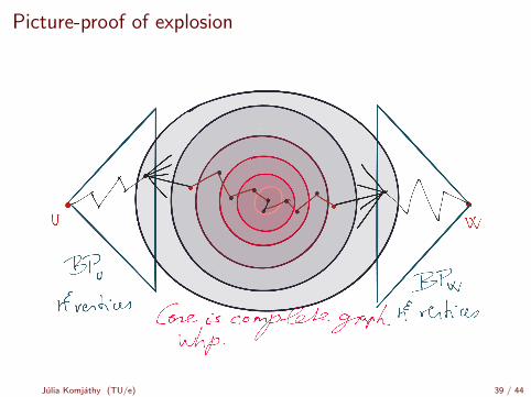
Picture-proof of explosion
Julia Komjathy (TU/e) 39 / 44

Picture-proof of explosion
Julia Komjathy (TU/e) 39 / 44

Picture-proof of explosion
Julia Komjathy (TU/e) 39 / 44

Picture-proof of explosion
Julia Komjathy (TU/e) 39 / 44

Picture-proof of explosion
Julia Komjathy (TU/e) 39 / 44

Picture-proof of explosion
Julia Komjathy (TU/e) 39 / 44
Picture-proof of explosion
Julia Komjathy (TU/e) 39 / 44
Picture-proof of explosion
Julia Komjathy (TU/e) 39 / 44

Picture-proof of explosion
Julia Komjathy (TU/e) 39 / 44

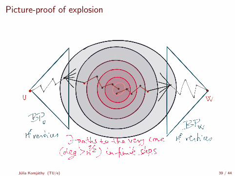
Non-picture-proof
Step 1: Couple the initial stages of the spreading by two independent agedependent BPs, one started at u, one at v , until generation Mn for somesmall Mn = o(log n).
Step 2: Use degree dependent percolation to percolate the whole graph:edges connecting vertices with degrees d1, d2 are kept iff their length is< tr(d1, d2) for some well-chosen threshold function.
Step 3: Find two vertices u, v with high enough percolated degree (sayKn) in the two BPs
Step 4: Show that in the percolated subgraph, there is a nested layeringstarting with degree Kn with the property that a vertex in layer i isconnected to at least one vertex in layer i + 1, and the degrees deg v in
layer i is ≈ K1/(τ−2)i
n .
Julia Komjathy (TU/e) 40 / 44

Non-picture-proof
Step 5: Show that u, v falls into layer 1. Thus
dL(u, v) ≥ dL(u, u) + dL(v , v) + 2
# layers∑i=1
F−1σ
(tr(K
1/(τ−2)i
n ,K1/(τ−2)i+1
n )).
Step 6: Show that the first two terms can be chosen to be negligible andthe second term is
(1 + ε)2
log log n/| log(τ−2)|∑i=1
F−1σ
(exp{−(τ − 2)−i}
).
Julia Komjathy (TU/e) 41 / 44

Thank you for the attention!
Julia Komjathy (TU/e) 42 / 44

Thank you for the attention!
Julia Komjathy (TU/e) 42 / 44

Thank you for the attention!
Julia Komjathy (TU/e) 42 / 44

Thank you for the attention!
Julia Komjathy (TU/e) 42 / 44

Explosive ‘extra’ weights on the configuration model
Theorem (Baroni, van der Hofstad, K)
Consider the configuration model with
power-law degree distribution with exponent τ ∈ (2, 3)
independent edge weights from distribution 1 + σ.
Then the sequence of random variables
d1+σ(u, v)− 2 log log n
| log(τ − 2)|is tight
if and only if the branching process BP(D?, σ) is explosive.
Xn is a tight sequence of random variables if the tail probabilities decayuniformly in n:∀ε > 0,∃Kε such that ∀n : P(|Xn| ≥ Kε) ≤ ε.
Julia Komjathy (TU/e) 43 / 44

4-line proof for non-tightness
Assume that the branching process BP(D?, σ) is conservative.
Every path from u to v uses at least dG (u, v) = d1(u, v) many edges,so
dG (u, v)− 2 log log n/| log(τ − 2)| is a tight sequenceFrom Hofstad, Hooghiemstra, Znamenski ‘07
σ non-explosive: dσ(u, v)→∞ by the previous theorem
As n→∞,
d1+σ(u, v)− 2 log log n
| log(τ − 2)|= O(1) + dσ(u, v)→∞
so the sequence cannot be tight.
Julia Komjathy (TU/e) 44 / 44

4-line proof for non-tightness
Assume that the branching process BP(D?, σ) is conservative.
Every path from u to v uses at least dG (u, v) = d1(u, v) many edges,so
d1+σ(u, v) ≥ dG (u, v) + dσ(u, v).
dG (u, v)− 2 log log n/| log(τ − 2)| is a tight sequenceFrom Hofstad, Hooghiemstra, Znamenski ‘07
σ non-explosive: dσ(u, v)→∞ by the previous theorem
As n→∞,
d1+σ(u, v)− 2 log log n
| log(τ − 2)|= O(1) + dσ(u, v)→∞
so the sequence cannot be tight.
Julia Komjathy (TU/e) 44 / 44

4-line proof for non-tightness
Assume that the branching process BP(D?, σ) is conservative.
Every path from u to v uses at least dG (u, v) = d1(u, v) many edges,so
d1+σ(u, v) ≥ 2 log log n
| log(τ − 2)|+ O(1) + dσ(u, v).
dG (u, v)− 2 log log n/| log(τ − 2)| is a tight sequenceFrom Hofstad, Hooghiemstra, Znamenski ‘07
σ non-explosive: dσ(u, v)→∞ by the previous theorem
As n→∞,
d1+σ(u, v)− 2 log log n
| log(τ − 2)|= O(1) + dσ(u, v)→∞
so the sequence cannot be tight.
Julia Komjathy (TU/e) 44 / 44