exploring the design space of deep convolutional … the design space of deep convolutional neural...

Exploring the Design Space of Deep Convolutional NeuralNetworks at Large Scale

Forrest Iandola

Electrical Engineering and Computer SciencesUniversity of California at Berkeley

Technical Report No. UCB/EECS-2016-207http://www2.eecs.berkeley.edu/Pubs/TechRpts/2016/EECS-2016-207.html

December 16, 2016

Copyright © 2016, by the author(s).All rights reserved.

Permission to make digital or hard copies of all or part of this work forpersonal or classroom use is granted without fee provided that copies arenot made or distributed for profit or commercial advantage and that copiesbear this notice and the full citation on the first page. To copy otherwise, torepublish, to post on servers or to redistribute to lists, requires priorspecific permission.

Exploring the Design Space ofDeep Convolutional Neural Networks at Large Scale

by

Forrest Iandola

B.S. University of Illinois at Urbana-Champaign, 2012

A dissertation submitted in partial satisfactionof the requirements for the degree of

Doctor of Philosophy

in

Electrical Engineering and Computer Sciences

in the

GRADUATE DIVISION

of the

UNIVERSITY OF CALIFORNIA, BERKELEY

Committee in charge:

Professor Kurt Keutzer, ChairProfessor Sara McMainsProfessor Krste Asanovic

Fall 2016

The dissertation of Forrest Iandola is approved.

Chair Date

Date

Date

University of California, BerkeleyFall 2016


Copyright c© 2016

by

Forrest Iandola

Abstract


by

Forrest Iandola

Doctor of Philosophy in Electrical Engineering and Computer Sciences

University of California, Berkeley

Professor Kurt Keutzer, Chair

In recent years, the research community has discovered that deep neural networks (DNNs) andconvolutional neural networks (CNNs) can yield higher accuracy than all previous solutions to abroad array of machine learning problems. To our knowledge, there is no single CNN/DNN ar-chitecture that solves all problems optimally. Instead, the “right” CNN/DNN architecture variesdepending on the application at hand. CNN/DNNs comprise an enormous design space. Quan-titatively, we find that a small region of the CNN design space contains 30 billion different CNNarchitectures.

In this dissertation, we develop a methodology that enables systematic exploration of the designspace of CNNs. Our methodology is comprised of the following four themes.

1. Judiciously choosing benchmarks and metrics.

2. Rapidly training CNN models.

3. Defining and describing the CNN design space.

4. Exploring the design space of CNN architectures.

Taken together, these four themes comprise an effective methodology for discovering the “right”CNN architectures to meet the needs of practical applications.

Professor Kurt KeutzerDissertation Committee Chair

1

To my wife, Dr. Steena Monteiro.

i

Contents

Contents ii

List of Figures iv

List of Tables v

1 Introduction and Motivation 1

1.1 Motivating the search for the “right” Deep Neural Network (DNN) architecture . . . 1

1.2 Ingredients for success in deep learning . . . . . . . . . . . . . . . . . . . . . . . . . . 4

1.3 The MESCAL Methodology for Design Space Exploration . . . . . . . . . . . . . . . 7

1.4 Organization of this dissertation . . . . . . . . . . . . . . . . . . . . . . . . . . . . . 9

1.5 How this dissertation relates to my prior work . . . . . . . . . . . . . . . . . . . . . . 10

2 Comprehensively defining benchmarks and metrics to evaluate DNNs 12

2.1 Finding the most computationally-intensiveDNN benchmarks . . . . . . . . . . . . . . . . . . . . . . . . . . . . . . . . . . . . . . 13

2.2 Transfer learning: amortizing a few large labeled datasets over many applications . . 17

2.3 Beyond accuracy: metrics for evaluating key properties of DNNs . . . . . . . . . . . 18

2.4 Orchestrating engineering teams to target specific DNN benchmarks and metrics . . 26

2.5 Relationship of our approach to the MESCAL methodology . . . . . . . . . . . . . . 29

3 Rapidly training DNNs on compute clusters 30

3.1 The need for efficient and scalable DNN training . . . . . . . . . . . . . . . . . . . . 30

3.2 Hardware for scalable DNN training . . . . . . . . . . . . . . . . . . . . . . . . . . . 32

3.3 Preliminaries and terminology . . . . . . . . . . . . . . . . . . . . . . . . . . . . . . . 32

3.4 Parallelism strategies . . . . . . . . . . . . . . . . . . . . . . . . . . . . . . . . . . . . 34

3.5 Choosing DNN architectures to accelerate . . . . . . . . . . . . . . . . . . . . . . . . 36

3.6 Implementing efficient data parallel training . . . . . . . . . . . . . . . . . . . . . . . 37

ii

3.7 Evaluation of FireCaffe-accelerated training on ImageNet . . . . . . . . . . . . . . . 41

3.8 Complementary approaches to accelerate DNN training . . . . . . . . . . . . . . . . 46

3.9 Conclusions . . . . . . . . . . . . . . . . . . . . . . . . . . . . . . . . . . . . . . . . . 47

4 Defining and describing the design space of DNN architectures 48

4.1 Introduction . . . . . . . . . . . . . . . . . . . . . . . . . . . . . . . . . . . . . . . . . 48

4.2 Key building blocks of CNN architectures . . . . . . . . . . . . . . . . . . . . . . . . 50

4.3 Understanding the dimensionality of CNN layers . . . . . . . . . . . . . . . . . . . . 57

4.4 A mental model for how CNN dimensions impact the quantity of computation andother metrics . . . . . . . . . . . . . . . . . . . . . . . . . . . . . . . . . . . . . . . . 58

4.5 Local changes to CNN architectures . . . . . . . . . . . . . . . . . . . . . . . . . . . . 60

4.6 Global changes to CNN architectures . . . . . . . . . . . . . . . . . . . . . . . . . . . 72

4.7 Intuition on the size of the design space of CNNs . . . . . . . . . . . . . . . . . . . . 76

4.8 The design space of techniques for training CNNs . . . . . . . . . . . . . . . . . . . . 77

4.9 Conclusions . . . . . . . . . . . . . . . . . . . . . . . . . . . . . . . . . . . . . . . . . 79

5 Exploring the design space of DNN architectures 81

5.1 Introduction and motivation . . . . . . . . . . . . . . . . . . . . . . . . . . . . . . . . 81

5.2 Related work . . . . . . . . . . . . . . . . . . . . . . . . . . . . . . . . . . . . . . . . 82

5.3 SqueezeNet: preserving accuracy withfew parameters . . . . . . . . . . . . . . . . . . . . . . . . . . . . . . . . . . . . . . . 84

5.4 Evaluation of SqueezeNet . . . . . . . . . . . . . . . . . . . . . . . . . . . . . . . . . 87

5.5 CNN Microarchitecture design space exploration . . . . . . . . . . . . . . . . . . . . 89

5.6 CNN Macroarchitecture design space exploration . . . . . . . . . . . . . . . . . . . . 92

5.7 Conclusions . . . . . . . . . . . . . . . . . . . . . . . . . . . . . . . . . . . . . . . . . 93

6 Conclusions 95

6.1 Contributions . . . . . . . . . . . . . . . . . . . . . . . . . . . . . . . . . . . . . . . . 95

6.2 Impact of our FireCaffe work on accelerating CNN/DNN training . . . . . . . . . . . 98

6.3 Impact of our work on exploring the design space of CNN architectures . . . . . . . 101

iii

List of Figures

1.1 Machine learning in 2012 . . . . . . . . . . . . . . . . . . . . . . . . . . . . . . . . . 2

1.2 Machine learning in 2016 . . . . . . . . . . . . . . . . . . . . . . . . . . . . . . . . . 3

1.3 Considerations when designing DNNs to use in practical applications . . . . . . . . . 3

1.4 Ingredients for success with deep neural networks . . . . . . . . . . . . . . . . . . . . 5

1.5 Impact of training set size on a DNN’s accuracy . . . . . . . . . . . . . . . . . . . . 6

2.1 The difference in single-GPU training times across different DNN applications. . . . 14

2.2 Multicore CPU server . . . . . . . . . . . . . . . . . . . . . . . . . . . . . . . . . . . 22

2.3 Implementing autonomous driving . . . . . . . . . . . . . . . . . . . . . . . . . . . . 27

3.1 Anatomy of a convolution layer. . . . . . . . . . . . . . . . . . . . . . . . . . . . . . . 33

3.2 Data parallel DNN training in FireCaffe . . . . . . . . . . . . . . . . . . . . . . . . . 35

3.3 Deep neural network architectures with more parameters do not necessarily deliverhigher accuracy. . . . . . . . . . . . . . . . . . . . . . . . . . . . . . . . . . . . . . . . 37

3.4 Illustrating how parameter servers and reduction trees communicate weight gradients 40

3.5 Comparing communication overhead with a parameter server vs. a reduction tree . . 40

3.6 Impact of learning rate on GoogLeNet accuracy . . . . . . . . . . . . . . . . . . . . . 45

4.1 Network-in-Network (NiN) . . . . . . . . . . . . . . . . . . . . . . . . . . . . . . . . . 49

4.2 Dimensions of a convolution layer. . . . . . . . . . . . . . . . . . . . . . . . . . . . . 51

4.3 Pooling with stride=1 . . . . . . . . . . . . . . . . . . . . . . . . . . . . . . . . . . . 53

4.4 Pooling with stride=2 . . . . . . . . . . . . . . . . . . . . . . . . . . . . . . . . . . . 54

5.1 Microarchitectural view of the Fire module . . . . . . . . . . . . . . . . . . . . . . . 85

5.2 Macroarchitectural view of the SqueezeNet architecture . . . . . . . . . . . . . . . . 86

5.3 Squeeze ratio, model size, and accuracy . . . . . . . . . . . . . . . . . . . . . . . . . 91

5.4 pct3x3, model size, and accuracy . . . . . . . . . . . . . . . . . . . . . . . . . . . . . . 92

iv

List of Tables

1.1 Organization of this dissertation. . . . . . . . . . . . . . . . . . . . . . . . . . . . . . 9

2.1 Training times and quantities of data in large-scale DNN application domains . . . . 13

2.2 Which aspects of a DNN-based system are evaluated by each metric? . . . . . . . . . 19

3.1 Volumes of data and computation for widely-used CNN/DNN architectures . . . . . 35

3.2 Accelerating the training of midsized deep models on ImageNet-1k. . . . . . . . . . . 44

3.3 Accelerating the training of ultra-deep, computationally intensive models onImageNet-1k. . . . . . . . . . . . . . . . . . . . . . . . . . . . . . . . . . . . . . . . . 46

4.1 Summary of local and global changes to CNN architectures . . . . . . . . . . . . . . 60

4.2 Dimensions of the NiN CNN architecture . . . . . . . . . . . . . . . . . . . . . . . . 62

4.3 NiN architecture with 4x more input channels . . . . . . . . . . . . . . . . . . . . . . 65

4.4 NiN architecture with 4x more filters in conv8 . . . . . . . . . . . . . . . . . . . . . . 67

4.5 NiN architecture with 4x larger filter resolution in one layer . . . . . . . . . . . . . . 69

4.6 NiN architecture with 4x more categories to classify . . . . . . . . . . . . . . . . . . 71

4.7 NiN architecture with pool3 removed . . . . . . . . . . . . . . . . . . . . . . . . . . . 73

4.8 NiN architecture with 4x larger input data resolution . . . . . . . . . . . . . . . . . . 75

4.9 A CNN architect is responsible for considering and exploring these design choices. . 78

5.1 SqueezeNet architectural dimensions . . . . . . . . . . . . . . . . . . . . . . . . . . . 88

5.2 Comparing SqueezeNet to model compression approaches . . . . . . . . . . . . . . . 89

5.3 SqueezeNet accuracy and model size using different macroarchitecture configurations. 93

v

Chapter 1

Introduction and Motivation

1.1 Motivating the search for the “right” Deep Neural Network

(DNN) architecture

Thus far, most computer science research and development has focused on problems for whicha mathematical solution or clear step-by-step procedure can be derived. These approaches arefeasible in popular computer science topics and applications including databases, numerical linearalgebra, encryption, and programming systems. However, there is an extremely broad space ofimportant problems for which no closed-form solution is known. What is the right equation totake pixels of an image and understand its contents? What equation should we use to take audiofrequencies and interpret speech? Nature and evolution has developed solutions to some of theseproblems, but so far there is no foolproof mathematical solution or series of steps that we canwrite down that will comprehensively solve these problems. For problems where no procedural ormathematical solution is known, we often turn to machine learning (ML), which we can broadlydefine as enabling the computer to automatically learn without explicitly being programmed.

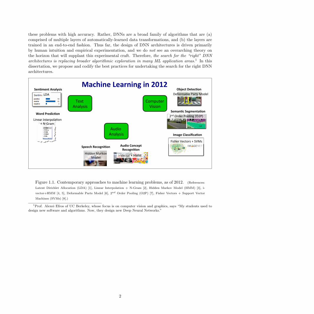
Over its history, the field of machine learning has churned out numerous approaches includingdecision trees, clustering, hidden Markov models (HMMs), support vector machines (SVMs), andneural networks. Given a new problem for which no mathematical/procedural solution is known,machine learning practitioners have often done some combination of (a) experimenting with severalfamilies of machine learning algorithms, and (b) attempting to design new algorithms. In Figure 1.1,we show a number of widely-studied machine learning problems, along with high-accuracy solutionsto these problems as of 2012.

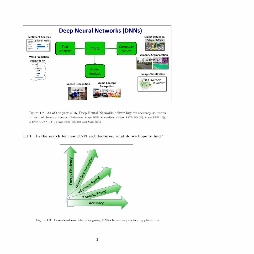
Since 2012, we have had the opportunity to play a role in the dramatic transformation inthe landscape of machine learning algorithms. Over the last few years, the machine learningcommunity has discovered that deep neural networks (DNNs) can give higher accuracy than allprevious solutions to a broad array of ML problems. Compared to Figure 1.1, notice that as ofthe year 2016 (Figure 1.2), the highest-accuracy solutions to these problems are based on DNNs.However, that’s not to say that a single DNN configuration is able to singlehandedly solve all of

1

these problems with high accuracy. Rather, DNNs are a broad family of algorithms that are (a)comprised of multiple layers of automatically-learned data transformations, and (b) the layers aretrained in an end-to-end fashion. Thus far, the design of DNN architectures is driven primarilyby human intuition and empirical experimentation, and we do not see an overarching theory onthe horizon that will supplant this experimental craft. Therefore, the search for the “right” DNNarchitectures is replacing broader algorithmic exploration in many ML application areas.1 In thisdissertation, we propose and codify the best practices for undertaking the search for the right DNNarchitectures.

Machine(Learning(in(2012(

Computer)Vision)

Audio)Analysis)

Text)Analysis)

Deformable)Parts)Model)

2nd)Order)Pooling)(O2P))

Fisher)Vectors)+)SVMs)

Hidden)Markov))Model)

Speech(Recogni3on( Audio(Concept((Recogni3on(

iGVector)+)HMM)

Object(Detec3on(

Seman3c(Segmenta3on(

Image(Classifica3on(

LDA)

Word(Predic3on(

Linear)InterpolaJon)+)NGGram)

Sen3ment(Analysis(

[1])F.(Iandola,)M.)Moskewicz,)K.)Keutzer.)libHOG:)EnergyGEfficient)Histogram)of)Oriented)Gradient)ComputaJon.)ITSC,)2015.)[2])N.)Zhang,)R.)Farrell,)F.(Iandola,)and)T.)Darrell.)Deformable)Part)Descriptors)for)FineGgrained)RecogniJon)and)A\ribute)PredicJon.)ICCV,)2013.))[3])M.)Kamali,)I.)Omer,)F.)Iandola,)E.)Ofek,)and)J.C.)Hart.)Linear)Clu\er)Removal)from)Urban)Panoramas))InternaJonal)Symposium)on)Visual)CompuJng.)ISVC,)2011.)))

Figure 1.1. Contemporary approaches to machine learning problems, as of 2012. (References:

Latent Dirichlet Allocation (LDA) [1], Linear Interpolation + N-Gram [2], Hidden Markov Model (HMM) [3], i-

vector+HMM [4, 5], Deformable Parts Model [6], 2nd Order Pooling (O2P) [7], Fisher Vectors + Support Vector

Machines (SVMs) [8].)

1Prof. Alexei Efros of UC Berkeley, whose focus is on computer vision and graphics, says “My students used todesign new software and algorithms. Now, they design new Deep Neural Networks.”

2

Deep$Neural$Networks$(DNNs)$

DNN# Computer#Vision#

Audio#Analysis#

Text#Analysis#

169layer#R9CNN#

199layer#FCN#

1529layer#CNN#

LSTM#NN#

Speech$Recogni8on$ Audio$Concept$$Recogni8on$

49layer#DNN#

Object$Detec8on$

Seman8c$Segmenta8on$

Image$Classifica8on$

39layer#RNN#

Word$Predic8on$word2vec#NN#

Sen8ment$Analysis$

[1]#K.#Ashraf,#B.#Elizalde,$F.$Iandola,#M.#Moskewicz,#J.#Bernd,#G.#Friedland,#K.#Keutzer.#Audio9Based#MulTmedia#Event#DetecTon#with#Deep#Neural#Nets#and#Sparse#Sampling.#ACM#ICMR,#2015.#[2]#F.$Iandola,#A.#Shen,#P.#Gao,#K.#Keutzer.#DeepLogo:#Hi[ng#logo#recogniTon#with#the#deep#neural#network#hammer.#arXiv:1510.02131,#2015.#[3]#F.$Iandola,#M.#Moskewicz,#S.#Karayev,#R.#Girshick,#T.#Darrell,#K.#Keutzer.#DenseNet:#ImplemenTng#Efficient#ConvNet#Descriptor#Pyramids.#arXiv:1404.1869,#2014.#[4]#R.#Girshick,#F.$Iandola,#T.#Darrell,#J.#Malik.#Deformable#Part#Models#are#ConvoluTonal#Neural#Networks.#CVPR,#2015.#[5]#H.#Fang,#S.#Gupta,#F.$Iandola,#et#al.#From#CapTons#to#Visual#Concepts#and#Back.#CVPR,#2015.###

Figure 1.2. As of the year 2016, Deep Neural Networks deliver highest-accuracy solutionsfor each of these problems. (References: 3-layer RNN [9], word2vec NN [10], LSTM NN [11], 4-layer DNN [12]),

16-layer R-CNN [13], 19-layer FCN [14], 152-layer CNN [15].)

1.1.1 In the search for new DNN architectures, what do we hope to find?Considera*ons+in+prac*cal+

deep+neural+network+applica*ons+

+++++++++++++++Energy+Efficien

cy+

Training+Spee

d+

Accuracy+

Figure 1.3. Considerations when designing DNNs to use in practical applications

3

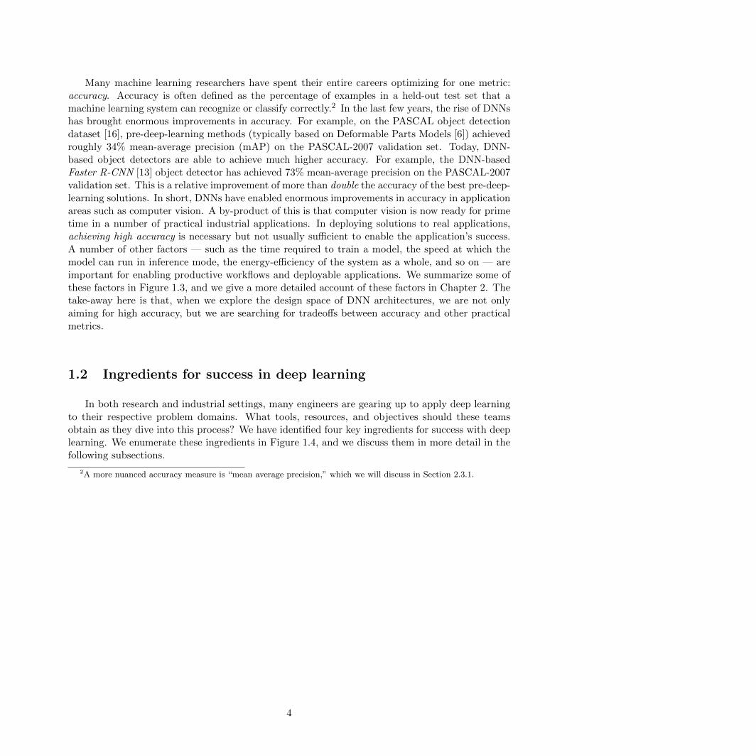
Many machine learning researchers have spent their entire careers optimizing for one metric:accuracy. Accuracy is often defined as the percentage of examples in a held-out test set that amachine learning system can recognize or classify correctly.2 In the last few years, the rise of DNNshas brought enormous improvements in accuracy. For example, on the PASCAL object detectiondataset [16], pre-deep-learning methods (typically based on Deformable Parts Models [6]) achievedroughly 34% mean-average precision (mAP) on the PASCAL-2007 validation set. Today, DNN-based object detectors are able to achieve much higher accuracy. For example, the DNN-basedFaster R-CNN [13] object detector has achieved 73% mean-average precision on the PASCAL-2007validation set. This is a relative improvement of more than double the accuracy of the best pre-deep-learning solutions. In short, DNNs have enabled enormous improvements in accuracy in applicationareas such as computer vision. A by-product of this is that computer vision is now ready for primetime in a number of practical industrial applications. In deploying solutions to real applications,achieving high accuracy is necessary but not usually sufficient to enable the application’s success.A number of other factors — such as the time required to train a model, the speed at which themodel can run in inference mode, the energy-efficiency of the system as a whole, and so on — areimportant for enabling productive workflows and deployable applications. We summarize some ofthese factors in Figure 1.3, and we give a more detailed account of these factors in Chapter 2. Thetake-away here is that, when we explore the design space of DNN architectures, we are not onlyaiming for high accuracy, but we are searching for tradeoffs between accuracy and other practicalmetrics.

1.2 Ingredients for success in deep learning

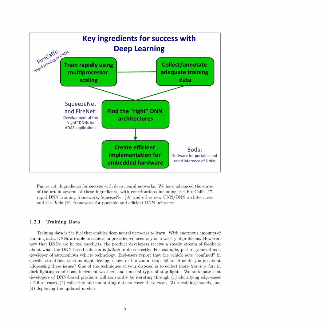
In both research and industrial settings, many engineers are gearing up to apply deep learningto their respective problem domains. What tools, resources, and objectives should these teamsobtain as they dive into this process? We have identified four key ingredients for success with deeplearning. We enumerate these ingredients in Figure 1.4, and we discuss them in more detail in thefollowing subsections.

2A more nuanced accuracy measure is “mean average precision,” which we will discuss in Section 2.3.1.

4

Key$ingredients$for$success$with$Deep$Learning$

Train$rapidly$using$mul9processor$

scaling$

Collect/annotate$adequate$training$

data$

Find$the$"right"$DNN$architectures$

Create$efficient$implementa9on$for$embedded$hardware$

SqueezeNet(and(FireNet:(Development(of(the("right"(DNNs(for(ADAS(applica=ons((

Boda:((So?ware(for(portable(and((rapid(inference(of(DNNs(

(

Figure 1.4. Ingredients for success with deep neural networks. We have advanced the state-of-the art in several of these ingredients, with contributions including the FireCaffe [17]rapid DNN training framework, SqueezeNet [18] and other new CNN/DNN architectures,and the Boda [19] framework for portable and efficient DNN inference.

1.2.1 Training Data

Training data is the fuel that enables deep neural networks to learn. With enormous amounts oftraining data, DNNs are able to achieve unprecedented accuracy on a variety of problems. However,now that DNNs are in real products, the product developers receive a steady stream of feedbackabout what the DNN-based solution is failing to do correctly. For example, picture yourself as adeveloper of autonomous vehicle technology. End-users report that the vehicle acts “confused” inspecific situations, such as night driving, snow, or horizontal stop lights. How do you go aboutaddressing these issues? One of the techniques at your disposal is to collect more training data indark lighting conditions, inclement weather, and unusual types of stop lights. We anticipate thatdevelopers of DNN-based products will constantly be iterating through (1) identifying edge-cases/ failure cases, (2) collecting and annotating data to cover these cases, (3) retraining models, and(4) deploying the updated models.

5

0 200 400 600 800 1000 12001umber of examples per class (linear)

0.0

0.1

0.2

0.3

0.4

0.5

0.6Top

-1 a

ccu

racy

0

Figure S1: Top-1 validation accuracy for networks trained on datasets containing reduced numbersof examples. The largest dataset contains the entire ILSVRC2012 (Deng et al., 2009) release witha maximum of 1300 examples per class, and the smallest dataset contains only 1 example per class(1000 data points in total). Top: linear axes. The slope of the rightmost line segment between 1000and 1300 is nearly zero, indicating that the amount of overfit is slight. In this region the validationaccuracy rises by 0.010820 from 0.54094 to 0.55176. Bottom: logarithmic axes. It is interesting tonote that even the networks trained on a single example per class or two examples per class manageto attain 3.8% or 4.4% accuracy, respectively. Networks trained on {5,10,25,50,100} examples perclass exhibit poor convergence and attain only chance level performance.

same 1000 classes as ImageNet, but where each class contained a maximum of n examples, foreach n 2 {1300, 1000, 750, 500, 250, 100, 50, 25, 10, 5, 2, 1}. The case of n = 1300 is the completeImageNet dataset.

Because occupying a whole GPU for this long was infeasible given our available computing re-sources, we also devised a set of hyperparameters to allow faster learning by boosting the learningrate by 25% to 0.0125, annealing by a factor of 10 after only 64,000 iterations, and stopping after200,000 iterations. These selections were made after looking at the learning curves for the base caseand estimating at which points learning had plateaued and thus annealing could take place. Thisfaster training schedule was only used for the experiments in this section. Each run took just over 4days on a K20 GPU.

The results of this experiment are shown in Figure S1 and Table S1. The rightmost few points in thetop subplot of Figure S1 appear to converge, or nearly converge, to an asymptote, suggesting thatvalidation accuracy would not improve significantly when using an AlexNet model with much moredata, and thus, that the degree of overfit is not severe.

2

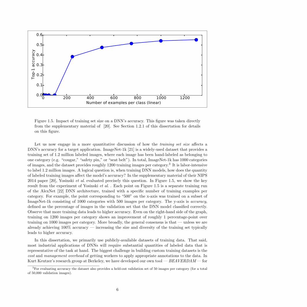
Figure 1.5. Impact of training set size on a DNN’s accuracy. This figure was taken directlyfrom the supplementary material of [20]. See Section 1.2.1 of this dissertation for detailson this figure.

Let us now engage in a more quantitative discussion of how the training set size affects aDNN’s accuracy for a target application. ImageNet-1k [21] is a widely-used dataset that provides atraining set of 1.2 million labeled images, where each image has been hand-labeled as belonging toone category (e.g. “cougar,” “safety pin,” or “seat belt”). In total, ImageNet-1k has 1000 categoriesof images, and the dataset provides roughly 1200 training images per category.3 It is labor-intensiveto label 1.2 million images. A logical question is, when training DNN models, how does the quantityof labeled training images affect the model’s accuracy? In the supplementary material of their NIPS2014 paper [20], Yosinski et al. evaluated precisely this question. In Figure 1.5, we show the keyresult from the experiment of Yosinski et al. . Each point on Figure 1.5 is a separate training runof the AlexNet [22] DNN architecture, trained with a specific number of training examples percategory. For example, the point corresponding to “500” on the x-axis was trained on a subset ofImageNet-1k consisting of 1000 categories with 500 images per category. The y-axis is accuracy,defined as the percentage of images in the validation set that the DNN model classified correctly.Observe that more training data leads to higher accuracy. Even on the right-hand side of the graph,training on 1200 images per category shows an improvement of roughly 1 percentage-point overtraining on 1000 images per category. More broadly, the general consensus is that — unless we arealready achieving 100% accuracy — increasing the size and diversity of the training set typicallyleads to higher accuracy.

In this dissertation, we primarily use publicly-available datasets of training data. That said,most industrial applications of DNNs will require substantial quantities of labeled data that isrepresentative of the task at hand. The biggest challenge in building custom training datasets is thecost and management overhead of getting workers to apply appropriate annotations to the data. InKurt Keutzer’s research group at Berkeley, we have developed our own tool — BEAVERDAM — for

3For evaluating accuracy the dataset also provides a held-out validation set of 50 images per category (for a totalof 50,000 validation images).

6

enabling human annotators to efficiently label large quantities of training data. More informationabout BEAVERDAM is available in [23, 24].

1.2.2 Rapid training

The ability to rapidly train DNN models is important for two reasons. First, rapid trainingenables developers to more quickly search for the “right” DNN models. Second, rapid trainingenables the workflow to keep up with ever-expanding training datasets. Enabling rapid training mayrequire some mix of: appropriate computational hardware, efficient implementations, appropriateDNN architectures, and (in many cases) efficient distributed computation over a cluster of servers.We will discuss our approaches for rapid DNN training in Chapter 3.

1.2.3 The right DNN models

The right models must give the “right” tradeoffs of efficiency metrics such as energy, computefootprint, memory footprint, all while achieving the accuracy level that is required by the end-application. We will discuss our approaches exploring DNN models and identifying the “right”DNN models in Chapter 5.

1.2.4 Efficient inference

Once we have the right models, we need to deploy them. There are opportunities for efficientimplementations on CPUs, GPUs, FPGAs, and ASICs / custom silicon. In all of these cases, weneed the right portable and efficient software implementation.

In this dissertation, we primarily rely on existing computational kernels such as those in theNVIDIA cuDNN library [25] for efficient DNN inference. The cuDNN kernels were developed by alarge team of engineers at NVIDIA, and they are highly efficient on NVIDIA hardware. However,the cuDNN kernels exclusively support NVIDIA processing hardware. Achieving high efficiencyfor DNN inference on other hardware (e.g. Intel, Texas Instruments, Qualcomm, AMD, and soon) remains a challenge for much of the research and industrial community. In joint work withMatthew Moskewicz, Ali Jannesari, and Kurt Keutzer of UC Berkeley, we developed the Bodasoftware framework. Boda provides DNN computational kernels that are competitive with cuDNNon NVIDIA hardware, and Boda’s kernels are also efficient on other hardware platforms such asQualcomm GPUs. More information about Boda is available in [19, 26].

1.3 The MESCAL Methodology for Design Space Exploration

So far, we have motivated the search for the “right” DNN architectures, and we have proposeda set of ingredients that are vital for carrying out this search. Now, what is the recipe book toleverage these raw ingredients to cook up new, world-beating deep neural network architectures?In this section, we begin to describe such a recipe book.

7

Deep Neural Networks comprise an enormous design space. An overarching theme and objec-tive of this dissertation is to design new DNN architectures and DNN-based systems that meetparticular design goals. While DNNs have only recently become widely studied, there are otherareas where broad design spaces have been fruitfully explored. One such area is computational hard-ware architecture, which comprises an enormous design space that has been continuously exploredby numerous semiconductor companies for more than 40 years. In this section, we summarize anumber of insights from hardware architectural design practices, and adapt them for DNNs.

In the broad design space of computational hardware, at one end of the spectrum lies the fixed-function circuit, and at the other end of the spectrum lies the general-purpose (GP) processor.Fixed-function circuits are routinely developed with the goal of providing cheap-to-manufacture4

energy-efficient and low-latency solutions for specific problems such as Bluetooth wireless commu-nication [27], network packet routing [28], and bitcoin mining [29].

One challenge is that, when a fixed-function circuit is designed to execute a particular algorithm,any future changes to the algorithm will likely require an entirely new circuit to be produced. On theother hand, general-purpose processors are relatively easy to program, with the ability to executea broad range of computations. But, a downside to GP processors is that they typically draw moreenergy (per computation performed) than a well-designed fixed-function circuit, and GP processorscan be more expensive to manufacture. So, what options lie between the two extremes of fixed-function circuits (highly efficient, cheap to manufacture, non-programmable) and general-purposeprocessors (less efficient, more expensive to manufacture, flexible to program)? Computationalhardware solutions in the middleground between fixed-function circuits and GP processors arecommonly called Application-Specific Processors (ASIPs).

Application-Specific Processors (ASIPs) have been developed for a variety of applications in-cluding speech recognition [30], computer vision [31], graphics [32], and software-defined wire-less [33]. Even for one given problem (e.g. creating a programmable chip for ethernet networkprocessing), there is a broad design space of ASIPs that can address this problem. This designspace include ASIPs that have already been produced/fabricated; designs that have been con-sidered but not fabricated; and designs that have not been considered at all. Each point in theASIP design space is a processor with unique characteristics such as the number of pipeline stages(depth), the number of processing elements, and the number of vector lanes. Each design pointalso has specific tradeoffs of energy-efficiency, throughput, latency, manufacturing cost, and othersuch metrics.

The MESCAL Methodology [34] codifies the best practices in navigating this design space to pro-duce high-quality ASIP hardware. The MESCAL methodology recommends beginning by choosingbenchmarks and target results on these benchmarks. Then, to achieve the desired results, a corner-stone of MESCAL is Design Space Exploration (DSE), which consists of identifying and evaluatinga broad range of points in the design space. In a series of case studies on ASIP hardware forethernet network processing, the MESCAL book [34] explores dimensions of the design space suchas the number of processing elements, the pipeline depth, and the width of vector lanes.

Broadly speaking, the characteristics of the ASIP design space have some commonalities withthe characteristics of the DNN design space. ASIPs and DNNs both comprise enormous designspaces. In practical deployments, the design spaces of both ASIPs and DNNs present tradeoffs interms of speed, energy, and other quality metrics (e.g. chip area in the case of ASIPs, and accuracy

4when produced in large quantities

8

in the case of DNNs). In the next section, we explain our MESCAL-inspired methodology forunderstanding and exploring the design space of DNN architectures.

1.4 Organization of this dissertation

In the MESCAL methodology [34] for exploring the design space of computational hardware,four of the central themes are:

• Judiciously using benchmarking

• Efficiently evaluate points the hardware design space

• Inclusively identify the architectural space

• Comprehensively explore the design space

After spending a number of years exploring the design space of DNNs, we have found thatthere are four MESCAL-like themes for DNN design space exploration (DSE). In the followingtable, we enumerate the DNN DSE themes, and for reference we include the analogous theme fromthe MESCAL methodology. In this dissertation, we devote one chapter to each of our DNN DSEthemes.

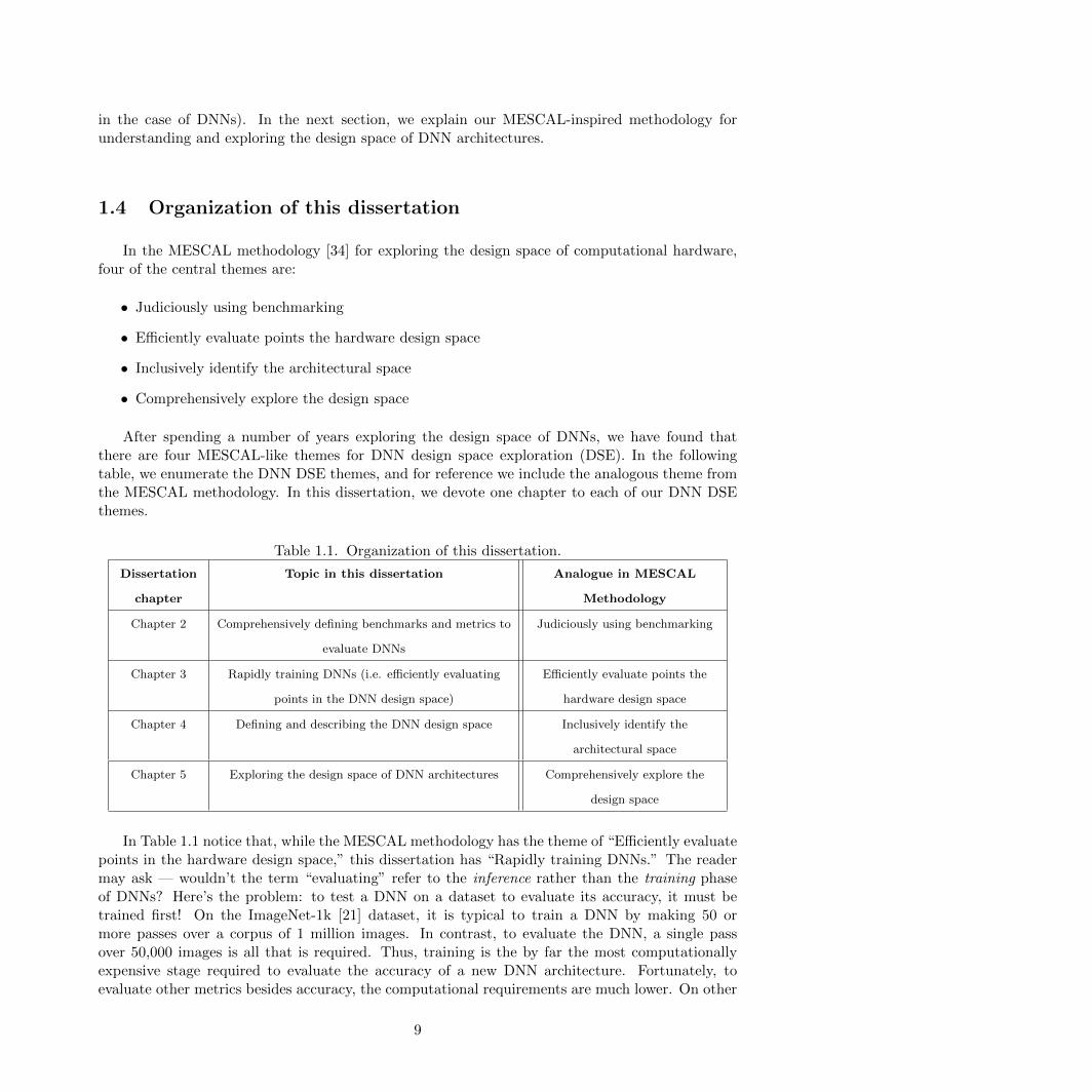
Table 1.1. Organization of this dissertation.

Dissertation

chapter

Topic in this dissertation Analogue in MESCAL

Methodology

Chapter 2 Comprehensively defining benchmarks and metrics to

evaluate DNNs

Judiciously using benchmarking

Chapter 3 Rapidly training DNNs (i.e. efficiently evaluating

points in the DNN design space)

Efficiently evaluate points the

hardware design space

Chapter 4 Defining and describing the DNN design space Inclusively identify the

architectural space

Chapter 5 Exploring the design space of DNN architectures Comprehensively explore the

design space

In Table 1.1 notice that, while the MESCAL methodology has the theme of “Efficiently evaluatepoints in the hardware design space,” this dissertation has “Rapidly training DNNs.” The readermay ask — wouldn’t the term “evaluating” refer to the inference rather than the training phaseof DNNs? Here’s the problem: to test a DNN on a dataset to evaluate its accuracy, it must betrained first! On the ImageNet-1k [21] dataset, it is typical to train a DNN by making 50 ormore passes over a corpus of 1 million images. In contrast, to evaluate the DNN, a single passover 50,000 images is all that is required. Thus, training is the by far the most computationallyexpensive stage required to evaluate the accuracy of a new DNN architecture. Fortunately, toevaluate other metrics besides accuracy, the computational requirements are much lower. On other

9

metrics such as training speed, inference speed, throughput (FLOPS/sec), and energy efficiency,DNNs can be evaluated using microbenchmarks that take a few seconds at the most. So, for anew DNN architecture, accuracy is the most computationally-intensive metric to evaluate, becausewe must train a neural net before we can evaluate its accuracy. In other words, when exploring abroad range of DNN architectures, training the model is the most acute computational bottleneckin evaluating each model.

1.5 How this dissertation relates to my prior work

To place this dissertation into context, it may be useful to briefly discuss the intellectual historyof this work.

I began my research career in the mid-2000s working on computational physics topics such asthe simulation of particle colliders [35]. I gradually moved into working on computational efficiencyaspects of physics simulations, working on physics-oriented distributed computing frameworks [36]as well as single-node acceleration [37]. Aside from computational physics, I also worked directly oncore parallel/efficient computing problems, such as the scheduling of tasks in single-GPU [38] andmulti-node or distributed [39, 40] environments, as well as the problem of estimating or predictingthe latency of sparse-matrix computations [41]. My early work on distributed scheduling was mo-tivated by maximizing computational efficiency, as well as guaranteeing hard real-time constraintsin safety-critical applications such as aircraft electronics. I later co-authored a paper directly onthe topic of aircraft electronics [42]. At the same time, I conducted research on computer visionapplications such as image stitching [43] and facial analysis [44].

My work at Berkeley has focused at the intersection of computer vision, machine learning,and computational efficiency. On the computational efficiency side, my work (with several keyco-authors) has spanned analyzing the energy-efficiency of computer vision algorithms [45], effi-cient feature extraction [46], amortizing the cost of DNN computation in object detection [47], andunifying efficiently-computed DNN features with other object detection approaches [48]. Convolu-tion is one of the most ubiquitous computational patterns in computer vision [49]. In 2013, our“communication-minimizing” GPU convolution kernels [50, 51] delivered a speedup of up to 8xover NVIDIA’s own NVIDIA Performance Primitives (NPP) library [52]. Since that time, NVIDIAhas developed more efficient convolution kernels in the cuDNN library [25], and key individu-als at NVIDIA tell us that the closed-source cuDNN implementation drew inspiration from ourcommunication-minimizing convolution approach. In 2016, in joint work with Matthew Moskewiczand Kurt Keutzer, we released a report on our Boda framework [19, 53], which provides efficient con-volution kernels and other software for efficient neural network computation. On NVIDIA GPUs,we found that Boda’s convolution efficiency is competitive with NVIDIA’s cuDNN software, andBoda also executes efficiently on GPUs from other vendors such as Qualcomm.

In addition, several of my contributions have focused developing more accurate approaches toproblems such as fine-grained visual classification [54], logo recognition [55], audio-based conceptrecognition [12], visual object detection [56], and image captioning [57].

In my final two years at Berkeley, I have focused on the problems of (a) accelerating the trainingof deep neural networks for computer vision [17, 58], and (b) understanding and exploring the designspace of deep neural networks [18]. Taken together, these contributions form the basis for a holisticstrategy for efficiently exploring the design space of deep neural network (DNN) architectures,

10

which is the focal point for this dissertation. In this dissertation, Chapter 3 is a refinement of ourFireCaffe [17] paper on accelerating DNN training, and Chapter 5 is a refinement of our SqueezeNetpaper [18], which not only introduced our novel SqueezeNet DNN architecture, but it also exploreda variety of DNN architectures of our own design. Chapters 1, 2, 4, and 6 are new discussions thatwe have not published in our previous work.

11

Chapter 2

Comprehensively defining benchmarks

and metrics to evaluate DNNs

For years, many computer architects evaluated their technology using a narrow set of bench-marks and metrics such as cycle count. While cycle count is a useful metric, the MESCAL book [34]contends that computer architectures must be evaluated on a representative set of benchmarks andmetrics. Ideally, these benchmarks and metrics should be representative of end-applications thatthe new computer architecture aims to enable. Like the old days of computer architecture when“cycle count” was erroneously considered to be a sufficient metric, machine learning and computervision research has predominantly focused on a single type of metric: accuracy. In the contextof computer vision, “accuracy” typically refers to the ability of a machine learning method tocorrectly classify, detect, segment, or otherwise understand visual imagery. However, now thatcomputer vision methods are becoming quite accurate, there a number of other metrics that mustbe considered when developing computer vision technology that will be deployed in real systems.Computer vision methods can be quite computationally intensive, and every application has explicitor implicit limits on factors such as: the speed that must be achieved, the quantity of energy thatis available, and the cost and quantity of hardware than can be used. In this chapter, we proposea more holistic set of metrics that enable a benchmarking methodology, which covers accuracy aswell as computational efficiency.

This chapter is organized as follows. First, in Section 2.1, we search for the mostcomputationally-intensive applications of DNNs. We discover that, when applying neural net-works to high-dimensional data such as images and video, the computational requirements can beextremely high. Next, in Section 2.2, we visit DNNs’ requirements for large quantities of expensivelabeled training data, and we describe how to alleviate some aspects of this problem with transferlearning. Then, in Section 2.3, we address the question: besides accuracy, what metrics are usefulfor evaluating DNNs that will be applied to practical applications? In Section 2.4, we describehow to use these benchmarks and metrics to evaluate an engineering team’s progress — as well asindividual engineers’ progress — toward the end-goal of achieving a specific tradeoff of accuracy

12

and efficiency. Finally, in Section 2.5, we describe how our metrics and benchmarking approachescompare to the MESCAL methodology [34].

2.1 Finding the most computationally-intensive

DNN benchmarks

When choosing representative benchmarks, it is not enough to identify the average case, middle-of-the-road benchmarks. Instead, our goal in choosing benchmarks is to identify the worst-case andmost challenging cases, and then to focus on optimizing for these cases. Applying this ideology tothe present topic, our goal is to take situations where DNN training and/or inference is currentlyintractably slow, and to use our computational efficiency skills to accelerate these DNN-basedapplications to run on a much faster time scale. With this in mind, we sought out the mostcomputationally time-consuming applications of DNNs. Specifically, we are looking for applicationswith the following two properties:

• Requirement 1. The total time to train a model is quite high.

• Requirement 2. The processing time per data sample during training or inference is quite high.

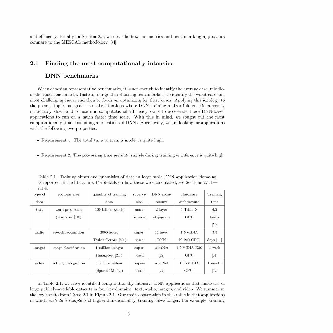
Table 2.1. Training times and quantities of data in large-scale DNN application domains,as reported in the literature. For details on how these were calculated, see Sections 2.1.1—2.1.4.

type of

data

problem area quantity of training

data

supervi-

sion

DNN archi-

tecture

Hardware

architecture

Training

time

text word prediction

(word2vec [10])

100 billion words unsu-

pervised

2-layer

skip-gram

1 Titan X

GPU

6.2

hours

[59]

audio speech recognition 2000 hours

(Fisher Corpus [60])

super-

vised

11-layer

RNN

1 NVIDIA

K1200 GPU

3.5

days [11]

images image classification 1 million images

(ImageNet [21])

super-

vised

AlexNet

[22]

1 NVIDIA K20

GPU

1 week

[61]

video activity recognition 1 million videos

(Sports-1M [62])

super-

vised

AlexNet

[22]

10 NVIDIA

GPUs

1 month

[62]

In Table 2.1, we have identified computationally-intensive DNN applications that make use oflarge publicly-available datasets in four key domains: text, audio, images, and video. We summarizethe key results from Table 2.1 in Figure 2.1. Our main observation in this table is that applicationsin which each data sample is of higher dimensionality, training takes longer. For example, training

13

text audio images videoData Type

100

101

102

103

Sin

gle

-GPU

Tra

inin

g T

ime (

log s

cale

)

Figure 2.1. The difference in single-GPU training times across different DNN applications.(See Table 2.1 for more details.)

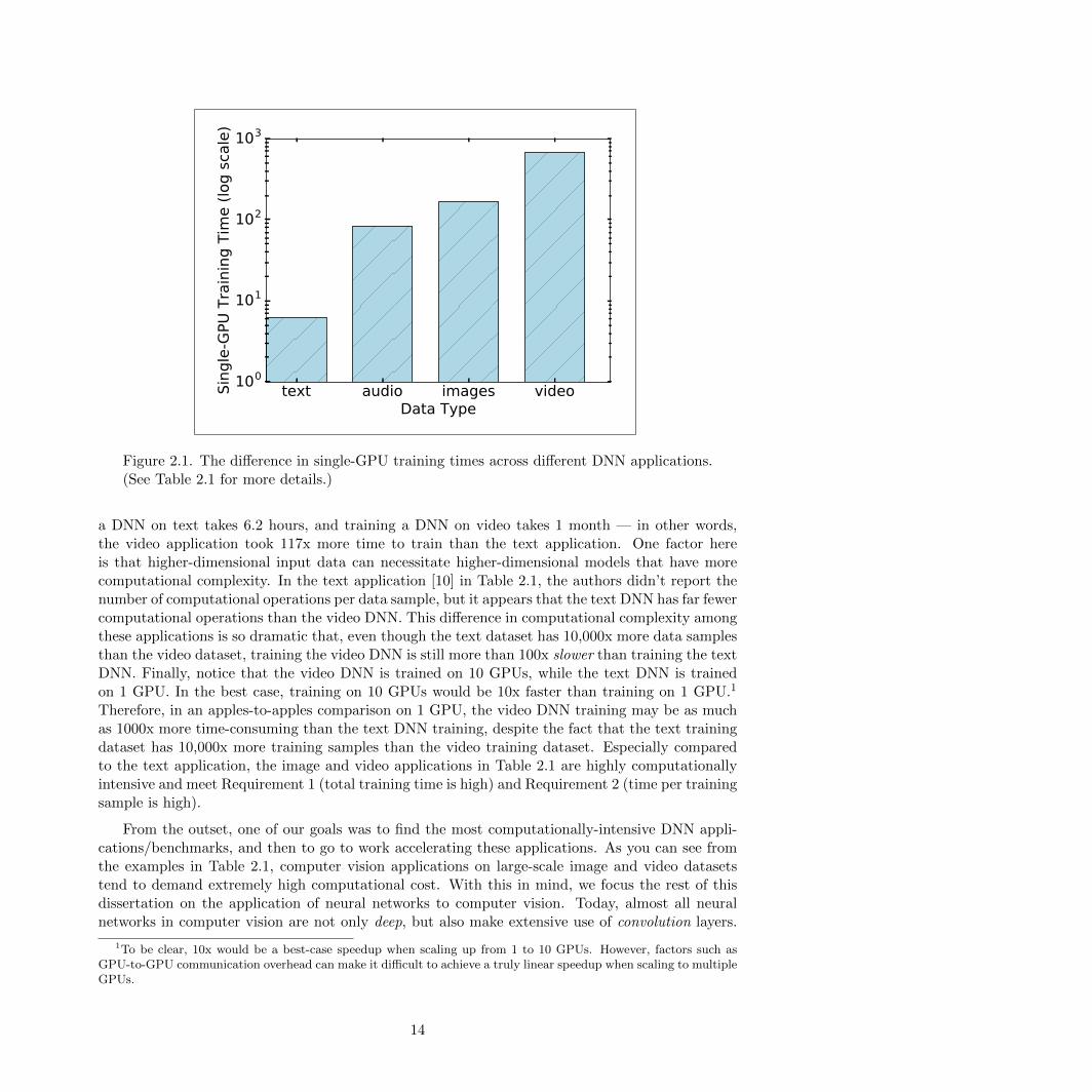
a DNN on text takes 6.2 hours, and training a DNN on video takes 1 month — in other words,the video application took 117x more time to train than the text application. One factor hereis that higher-dimensional input data can necessitate higher-dimensional models that have morecomputational complexity. In the text application [10] in Table 2.1, the authors didn’t report thenumber of computational operations per data sample, but it appears that the text DNN has far fewercomputational operations than the video DNN. This difference in computational complexity amongthese applications is so dramatic that, even though the text dataset has 10,000x more data samplesthan the video dataset, training the video DNN is still more than 100x slower than training the textDNN. Finally, notice that the video DNN is trained on 10 GPUs, while the text DNN is trainedon 1 GPU. In the best case, training on 10 GPUs would be 10x faster than training on 1 GPU.1

Therefore, in an apples-to-apples comparison on 1 GPU, the video DNN training may be as muchas 1000x more time-consuming than the text DNN training, despite the fact that the text trainingdataset has 10,000x more training samples than the video training dataset. Especially comparedto the text application, the image and video applications in Table 2.1 are highly computationallyintensive and meet Requirement 1 (total training time is high) and Requirement 2 (time per trainingsample is high).

From the outset, one of our goals was to find the most computationally-intensive DNN appli-cations/benchmarks, and then to go to work accelerating these applications. As you can see fromthe examples in Table 2.1, computer vision applications on large-scale image and video datasetstend to demand extremely high computational cost. With this in mind, we focus the rest of thisdissertation on the application of neural networks to computer vision. Today, almost all neuralnetworks in computer vision are not only deep, but also make extensive use of convolution layers.

1To be clear, 10x would be a best-case speedup when scaling up from 1 to 10 GPUs. However, factors such asGPU-to-GPU communication overhead can make it difficult to achieve a truly linear speedup when scaling to multipleGPUs.

14

In computer vision, deep convolutional neural networks are often referred to as DCNNs or simplyCNNs. From this point forward in the dissertation, we will primarily use the term CNN to describeneural networks applied to computer vision.

We now turn our attention back to Table 2.1. As you can probably imagine, summarizing fourdomains of DNN applications in one table requires many simplifications and omissions. In thefollowing subsections, we provide all the details of how the numbers in Table 2.1 were calculated. Ifyou feel satisfied with your understanding of Table 2.1, we recommend skipping ahead to Section 2.2.

2.1.1 Text (Least computationally intensive)

In the past, text analysis algorithms often relied on hand-engineered features such as n-grams.However, since the publication of the word2vec paper [10], Deep Neural Networks have gone intowidespread use for creating feature representations of text data. The word2vec approach has beenused to improve the accuracy of a number of text-based applications such as document search andinternet click prediction.

We now provide more background on the word2vec approach. Word2vec requires a large corpusof text data — for example many sentences collected from Wikipedia or other internet text. Unlikethe audio, imaging, and video topics discussed in this chapter, training word2vec on text datadoes not require human-annotated labels. Instead, the word2vec training problem is phrased in aself-supervised way. Then, for each sentence, we remove a word and ask the model to predict whatword best fits that sentence. The correct response from the model would be to predict the wordthat was in the original sentence. Any other response is considered wrong, and the correct responseis backpropagated through the model. Ultimately, this produces a model that can predict missingwords in sentences. This is self-supervised, because — rather than requiring a human annotator —the labels are derived from the corpus of training data. The research community has discoveredthat the representation learned in this training procedure is broadly applicable as a high-qualityfeature representation for a variety of problems.

How long does it take to train a word2vec model? The original word2vec paper trained itsmodel on a dataset that contained a total of 100 billion words [10]. The word2vec authors reportedtraining a word2vec model on 100 billion words in one day on a single server, but no informationis provided about the type of hardware used in this server. However, Zhao et al. [59] did reportthe amount of time required to train a word2vec model, as observed in their own experiments.Admittedly, it isn’t entirely clear whether the model by Zhou et al. has the same dimensions andconfiguration as the model presented in the original word2vec paper. Nevertheless, Zhao et al. [59]reported training a word2vec model on a single NVIDIA Titan X GPU at a rate of 4.5M wordsper second, which equates to roughly 6.2 hours to complete one epoch of training.2 We used thenumbers by Zhao et al. for the word2vec entry in Table 2.1.

2.1.2 Audio (Somewhat computationally intensive)

DNNs are now widely used in research and commercial speech recognition systems. In mostapproaches, training a DNN to perform speech recognition requires a large quantity of appropriate

2This is assuming one epoch (pass through the training set) is necessary to train a word2vec model.

15

training data. This training data is typically a corpus of spoken-word audio, which has been labeled(by human annotators) with words.3

To our knowledge, the largest publicly available corpus of word-labeled audio data is the FisherCorpus, which has 2000 hours of data [60]. So, how long does it take to train a high-accuracy DNNon this dataset? In the literature, we have not found any articles that report training times onthe Fisher Corpus. However, researchers at Baidu reported the time required to train on an evenlarger dataset. The Baidu researchers used a 12,000-hour dataset, which includes all 2000 hoursof the Fisher Corpus, plus 8600 hours of proprietary data collected and labeled by Baidu, plus anumber of smaller datasets such as WSJ [63], Switchboard [64], and LibriSpeech [65]. To train onthis 12,000-hour dataset using a single NVIDIA K1200 GPU, the authors reported that it takesapproximately 3 weeks to train a high-accuracy DNN model.4 Given that takes 3 weeks to trainon the full 12,000-hour Baidu dataset, and knowing that the Fisher Corpus contains 1

6 as muchtraining data, we estimate that it would take half a week (3.5 days) to train a high accuracy DNNusing the Fisher Corpus, which to our knowledge is the largest publicly-available dataset.5

2.1.3 Images (Very computationally intensive)

Image classification is a core problem in computer vision. The goal here is to automaticallyassign one or more labels to an image. If the image is zoomed-in on one primary object such asa dog, a valid classification label could be “dog” or even the specific breed of dog. If the image iszoomed-out on a scene, a reasonable label might be “park” or “office,” depending on the contentsof the image.

Researchers have developed large datasets of labeled data for training and evaluating imageclassification methods. One of the largest image classification datasets is ImageNet-1k, which has1000 categories of images, and an average of 1200 labeled training images per category, for a total of1.2 million labeled training images [21]. A CNN architecture called AlexNet [22] won the ImageNetimage classification competition in 2012. ImageNet is a large dataset, and CNNs are often quitecomputationally intensive.

So, how long does it take to train the AlexNet model on ImageNet-1k? Krizhevsky et al. [22]reported that this training took approximately 1 week. This result was achieved by training ona single NVIDIA K20 GPU using well-tuned computational kernels. The full ImageNet [21] datacorpus (of which ImageNet-1k is a modest subset) has at least 7 million images, where each imageis labeled as one of 22,000 categories [66]. On a fixed number of epochs6, training on the fullImageNet corpus should take 6x times longer, for a total of 6 weeks of execution between the timethe researcher begins training the model, and the time when the training is complete.7

Now, even larger image classification datasets have been developed. For example, the Places2scene classification dataset has over 8 million labeled images in the training set [67]. As datasets

3Alternatively, the corpus can be labeled with individual syllables called phonemes. However, word-labels havebeen used to train the current state-of-art speech recognition approaches.

4The Deep Speech 2 authors go on to present multi-GPU distributed training strategies to accelerate training.We will discuss distributed training in depth in Chapter 3.

5Given a fixed number of epochs (passes through the training set), DNN training time grows linear with thetraining set size.

6an “epoch” is one pass through the training set7This “6x” number comes from the fact that the full ImageNet dataset has 7M images rather than 1.2M images.

16

continue to grow, the training of DNNs is on track to become more and more computationallyexpensive.

2.1.4 Video (Extremely computationally intensive)

ImageNet-1k has slightly more than 1 million labeled images in its training set. However, theSports-1M dataset has nearly 1 million labeled videos in its training set [62]. Each video may becomprised of hundreds of frames per minute, and the average video in the dataset is 5.5 minuteslong. The labels for Sports-1M are rather coarse. Rather than labeling individual objects orindividual frames, the creators of Sports-1M opted to have just one label per video. Specifically,each video is labeled with a particular activity that is being performed in the video. The dataset iscalled Sports-1M, so the “activities” are types of sports — a total of 487 different types of sports, tobe exact. When training models on the Sports-1M dataset, the typical end-goal is to automaticallypredict one label (e.g. the type of sport being played) for each video in the test set.

How long does it take to train a model to recognize types of sports that are being played invideos? Karpathy et al. trained an AlexNet-based CNN model on the Sports-1M dataset [62].The authors trained the model using custom settings for the downsampling factor in the inputimages and the number of images or clips to use per training video. Rather than attempting tocalculate the training time based on the AlexNet-ImageNet experiments in the previous subsection,we simply report the training times from Karpathy et al. as follows. Karpathy et al. were able totrain a high-accuracy DNN model on Sports-1M in 1 month using a cluster of 10 GPUs.

2.2 Transfer learning: amortizing a few large labeled datasets over

many applications

In the previous section, we found that CNN/DNN training tends to be more time-consumingand computationally expensive in large-scale computer vision recognition problems on images andvideo, compared to text and audio which typically have less computational overhead. We havededicated the remainder of this dissertation to accelerating, rethinking, and improving the efficiencyand accuracy of CNNs applied to computer vision. A key element in many of today’s computervision CNN workflows is transfer learning, which we will discuss in the following paragraphs.

To achieve the highest possible accuracy, CNN/DNNs typically need a large supply of trainingdata.8 In computer vision, the state-of-art CNNs are often trained with supervised learning meth-ods. Supervised learning methods typically require the training data to be annotated by humans.A practical question is, how do we avoid the need to pay human annotators to annotate enormousdatasets for each new application for which we would like to develop high-accuracy CNN models?

Image classification is an application where training data is relatively inexpensive to gather.This is because, to train a CNN for image classification, we only need one label (e.g. “dog” or“office building”) for each image. In contrast, the problem of object detection is the problem ofautomatically localizing and classifying each object in an image. Typically, to train a CNN to

8We provided some quantitative numbers on how dataset size impacts accuracy in Section 1.2.1.

17

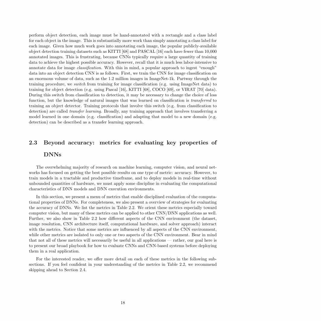
perform object detection, each image must be hand-annotated with a rectangle and a class labelfor each object in the image. This is substantially more work than simply annotating a class label foreach image. Given how much work goes into annotating each image, the popular publicly-availableobject detection training datasets such as KITTI [68] and PASCAL [16] each have fewer than 10,000annotated images. This is frustrating, because CNNs typically require a large quantity of trainingdata to achieve the highest possible accuracy. However, recall that it is much less labor-intensive toannotate data for image classification. With this in mind, a popular approach to ingest “enough”data into an object detection CNN is as follows. First, we train the CNN for image classification onan enormous volume of data, such as the 1.2 million images in ImageNet-1k. Partway through thetraining procedure, we switch from training for image classification (e.g. using ImageNet data) totraining for object detection (e.g. using Pascal [16], KITTI [68], COCO [69], or VIRAT [70] data).During this switch from classification to detection, it may be necessary to change the choice of lossfunction, but the knowledge of natural images that was learned on classification is transferred totraining an object detector. Training protocols that involve this switch (e.g. from classification todetection) are called transfer learning. Broadly, any training approach that involves transferring amodel learned in one domain (e.g. classification) and adapting that model to a new domain (e.g.detection) can be described as a transfer learning approach.

2.3 Beyond accuracy: metrics for evaluating key properties of

DNNs

The overwhelming majority of research on machine learning, computer vision, and neural net-works has focused on getting the best possible results on one type of metric: accuracy. However, totrain models in a tractable and productive timeframe, and to deploy models in real-time withoutunbounded quantities of hardware, we must apply some discipline in evaluating the computationalcharacteristics of DNN models and DNN execution environments.

In this section, we present a menu of metrics that enable disciplined evaluation of the computa-tional properties of DNNs. For completeness, we also present a overview of strategies for evaluatingthe accuracy of DNNs. We list the metrics in Table 2.2. We orient these metrics especially towardcomputer vision, but many of these metrics can be applied to other CNN/DNN applications as well.Further, we also show in Table 2.2 how different aspects of the CNN environment (the dataset,image resolution, CNN architecture itself, computational hardware, and solver approach) interactwith the metrics. Notice that some metrics are influenced by all aspects of the CNN environment,while other metrics are isolated to only one or two aspects of the CNN environment. Bear in mindthat not all of these metrics will necessarily be useful in all applications — rather, our goal here isto present our broad playbook for how to evaluate CNNs and CNN-based systems before deployingthem in a real application.

For the interested reader, we offer more detail on each of these metrics in the following sub-sections. If you feel confident in your understanding of the metrics in Table 2.2, we recommendskipping ahead to Section 2.4.

18

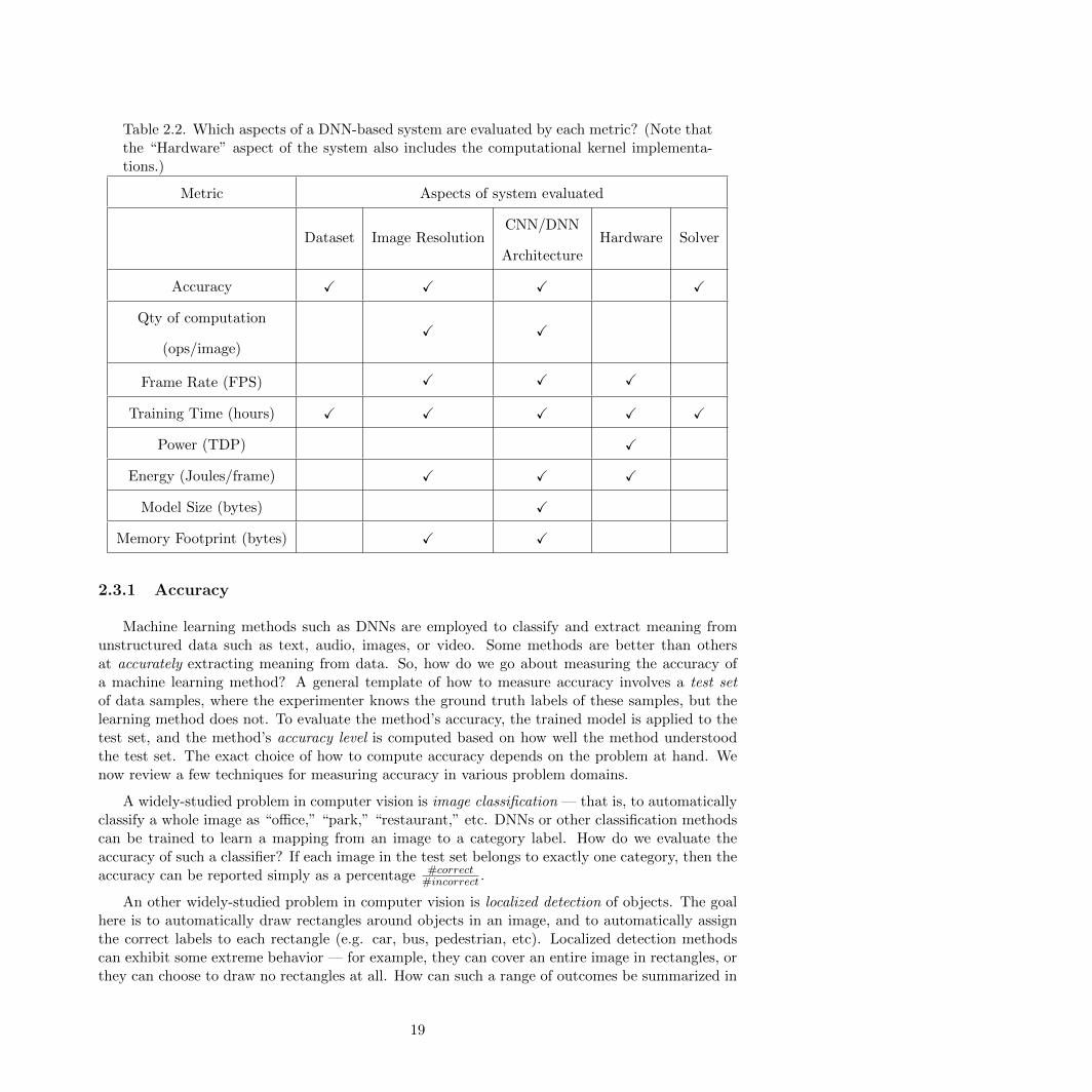
Table 2.2. Which aspects of a DNN-based system are evaluated by each metric? (Note thatthe “Hardware” aspect of the system also includes the computational kernel implementa-tions.)

Metric Aspects of system evaluated

Dataset Image ResolutionCNN/DNN

ArchitectureHardware Solver

Accuracy X X X X

Qty of computation

(ops/image)X X

Frame Rate (FPS) X X X

Training Time (hours) X X X X X

Power (TDP) X

Energy (Joules/frame) X X X

Model Size (bytes) X

Memory Footprint (bytes) X X

2.3.1 Accuracy

Machine learning methods such as DNNs are employed to classify and extract meaning fromunstructured data such as text, audio, images, or video. Some methods are better than othersat accurately extracting meaning from data. So, how do we go about measuring the accuracy ofa machine learning method? A general template of how to measure accuracy involves a test setof data samples, where the experimenter knows the ground truth labels of these samples, but thelearning method does not. To evaluate the method’s accuracy, the trained model is applied to thetest set, and the method’s accuracy level is computed based on how well the method understoodthe test set. The exact choice of how to compute accuracy depends on the problem at hand. Wenow review a few techniques for measuring accuracy in various problem domains.

A widely-studied problem in computer vision is image classification — that is, to automaticallyclassify a whole image as “office,” “park,” “restaurant,” etc. DNNs or other classification methodscan be trained to learn a mapping from an image to a category label. How do we evaluate theaccuracy of such a classifier? If each image in the test set belongs to exactly one category, then theaccuracy can be reported simply as a percentage #correct

#incorrect .

An other widely-studied problem in computer vision is localized detection of objects. The goalhere is to automatically draw rectangles around objects in an image, and to automatically assignthe correct labels to each rectangle (e.g. car, bus, pedestrian, etc). Localized detection methodscan exhibit some extreme behavior — for example, they can cover an entire image in rectangles, orthey can choose to draw no rectangles at all. How can such a range of outcomes be summarized in

19

a single metric of accuracy? There are number of approaches, most of which begin by organizingthe method’s detections into false positives (FP), true positives (TP), false negatives (FN), andtrue negatives (TN). With this information, metrics such as average precision (AP) [16] or falsepositives per image (FPPI) [71] can then be computed. Each of these metrics can summarize anobject detector’s accuracy in a single metric.

There are a number of additional metrics for calculating accuracy in other problem domains.The accuracy of semantic segmentation — that is, assigning object labels to all pixels in an image —is often evaluated with an Intersection over Union (IOU) metric [72]. The accuracy of speech recog-nition methods can be evaluated on a per-frame or per-word basis. Likewise, the accuracy of videoanalysis methods can be evaluated on a timescale ranging from per-frame to per-video [62]. Theaccuracy of methods for automatically assigning captions or sentences to images is commonly eval-uated with metrics such as Bilingual Evaluation Understudy (BLEU) [73] or Metric for Evaluationof Translation with Explicit ORdering (METEOR) [74]. In general terms, BLEU and METEOR aredesigned to quantify the correctness of the algorithmically generated caption’s word usage, wordordering, and number of words, with respect to a database of ground-truth captions. In opticalflow algorithms, the accuracy is often measured with an angular error [75] metric.

2.3.2 Quantity of Computation

Today’s DNN architectures present a wide range of computational requirements. For example,the LeNet [76] DNN architecture performs 5.74 million floating-point arithmetic operations (5.74MFLOPS) to classify a 28x28 image. At the other end of the spectrum, the VGG-19 [77] DNNarchitecture performs 117,000 MFLOPS to classify a 224x224 image. If applied to a 224x224 image,LeNet performs 2700 MFLOPS to classify the image.9 Applying VGG-19 to a 224x224 input imagerequires 20,000x more computation than applying LeNet to a 28x28 input image. Even with thesame input image size, VGG-19 requires 43x more computation than LeNet. DNNs comprise anenormous design space, and some points in this design space require orders of magnitude morecomputation than others.

So far, we have focused on the quantity of computation required to classify images during theinference phase. Now, we turn our attention to the quantity of computation needed to train aDNN. As a rule of thumb, the computation required per image when training a DNN is 3x morethan the computation required for inference [78]. As with inference, one way to think about thequantity of computation is in terms of OPS/frame.10 However, during training, multiple passesthrough the training set (epochs) are often performed. A good way to think about the quantity ofcomputation is to consider the total number of arithmetic operations required to complete training:(OPS/frame) ∗ (#frames in training set) ∗ (#epochs). While the number of epochs could beselected dynamically (e.g. stop training when the model reaches a convergence criterion), we haveobserved that most CNN researchers define a static number of epochs offline, prior to the trainingexperiment.

How does quantity of computation relate to the speed of execution? DNNs/CNNs are com-

9On a 28x28 image, the first fully-connected (FC) layer in LeNet has a operates on an input size of 4x4xChannels,and each filter is also 4x4xChannels. To adapt LeNet to a 224x224 image, we make this FC layer into a convolutionlayer with filters of size 4x4xChannels, and we average pool the output of this layer down to 1x1xChannels.

10Work by He and Sun [78] and Szegedy et al. [79] are examples of papers that report their CNN models’ accuracyas well as computation required per frame.

20

monly implemented with 32-bit floating-point math (so the OPS are FLOPS), and less commonlywith integer math (IOPS). A high-end GPU such as the NVIDIA P100 can perform up to 10.6TFLOPS/sec [80].11 If running at 10.6 TFLOPS/sec, LeNet (224x224 images) could classify 3900frames/sec12, while VGG-19 could classify just 91 frames/sec frames/sec.13 However, there is noguarantee than an off-the-shelf implementation will achieve the peak efficiency of 10.6 TFLOPS/sec.Well-tuned CNN libraries such as Boda [19], cuDNN [25], fbfft [81], and Neon [82] been shown toachieve 30-95% of peak, depending on the choice of hardware and the dimensions of each CNNlayer.

2.3.3 Quantity of Communication

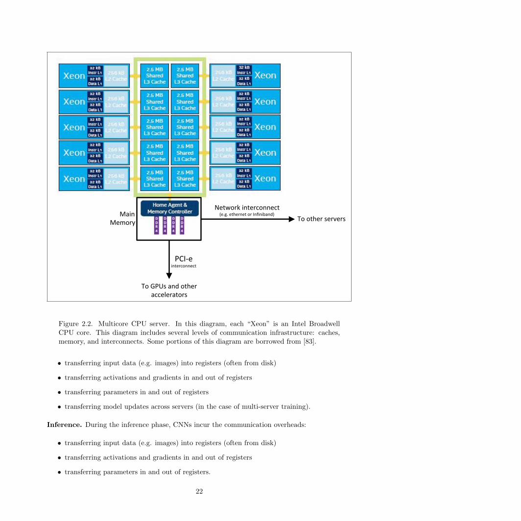
A computational resource (e.g. one mobile phone or a cluster of servers) has a limited quantityof computation that it can perform each second. However, an often-overlooked factor is that acomputational resource also has a limited quantity of communication that it can perform eachsecond. We define communication quite broadly. One variety of communication is the movementof data from one server to an other, for example using a hardware networking platform such asEthernet or Infiniband. An other variety of communication is within a server, between differentlayers of the storage and memory hierarchy. Thus, we classify all varieties of data movement ascommunication. We illustrate an example configuration of hardware pertaining to these levels ofdata movement in Figure 2.2.

In the landmark Roofline Model paper [84], Williams et al. showed that, depending on themethod and choice of hardware, the theoretical best-case execution time can be limited by eithercomputation or communication. We interpret this broadly to mean that any of the following canbe a limiting factor on the speed at which an algorithm/program can execute:

1. peak throughput computational hardware (influenced by factors such as the number of pro-cessors, width of vector lanes, clock speed, and pipeline depth), OR

2. peak bandwidth and latency of the memory hierarchy (typically within a server), OR

3. peak bandwidth and latency of interconnect between servers.

Note that we define peak to denote the theoretical best-case that can be achieved by a givenhardware unit.

With all of this in mind, we find that it is important to analyze not only the quantity ofcomputation, but also the quantity of communication required by a CNN architecture. Withspecific hardware and implementations, we can also study speed — i.e. “computation per second”and “communication per second,” and we will discuss this in the next section. But, before weget to that, let us briefly consider how the quantity of communication differs during training andinference of CNNs.

Training. During the training phase, CNNs incur the communication overheads:

11A processor’s highest achievable throughput is known as “peak” throughput.1210,600 peak GFLOPS/s / 2.7 GFLOPS per frame13where input frames are of size 224x224 for both VGG-19 and LeNet

21

3"

DeepScale Intel&Broadwell&

Reference"""www.nextpla0orm.com/2016/05/31/intel:lines:thunderx:arms:xeons/""author="Timothy"PrickeE"Morgan""journal="The"Next"Pla0orm""Jtle="Intel"Lines"Up"ThunderX"ARM"Against"Xeons","year="2016""""

capJon:"Diagram"of"an"Intel"Broadwell"mulJcore"CPU"server."This"diagram"focuses"on"the"communicaJon"infrastructure"::"caches,"memory,"and"interconnects.""Each"``Xeon""is"a"CPU"core."Some"aspects"of"this"diagram"are"courtesy"of"[REF"The"Next"Pla0orm"arJcle]."

Main""Memory"

Network"interconnect"(e.g."ethernet"or"Infiniband)"

To"other"servers"

PCI:e"interconnect"

To"GPUs"and"other""accelerators"

Figure 2.2. Multicore CPU server. In this diagram, each “Xeon” is an Intel BroadwellCPU core. This diagram includes several levels of communication infrastructure: caches,memory, and interconnects. Some portions of this diagram are borrowed from [83].

• transferring input data (e.g. images) into registers (often from disk)

• transferring activations and gradients in and out of registers

• transferring parameters in and out of registers

• transferring model updates across servers (in the case of multi-server training).

Inference. During the inference phase, CNNs incur the communication overheads:

• transferring input data (e.g. images) into registers (often from disk)

• transferring activations and gradients in and out of registers

• transferring parameters in and out of registers.

22

Unlike training, inference does not requite communication across servers because each data sample(e.g. image) can be processed independently, and the model is no longer being updated or modified.

2.3.4 Speed

The quantities of computation and communication are properties of a DNN architecture, butthese are orthogonal from the underlying hardware and implementation that executes the DNN.Speed is a more holistic metric that is impacted by a number of factors including the DNN archi-tecture, the software implementation, and the choice of computational hardware.

The following example illustrates the difference between measuring quantity of computationand measuring speed. During inference, the VGG-19 DNN performs 117 GFLOPS per frame —this is the quantity of computation. The majority (> 95%) of these FLOPS can be attributed toperforming convolution calculations. But, at what rate can we expect a processor to perform theseFLOPS? Every processor has a theoretical peak, or best-case, throughput in FLOPS/s. For example,an NVIDIA Titan X GPU has a theoretical peak of 6 TFLOPS/s. A study of high-performancecomputing applications implemented on supercomputers found that the average application runsat approximately 5% of the processor’s peak efficiency [85]. At a rate of 5% of 6 TFLOPS/s (i.e.0.03 TFLOPS/s), the inference phase of VGG would run at 0.25 frames/sec. However, as shown inour Boda work on accelerating convolutions on GPUs, it is feasible to implement certain problemsizes convolution at 50% of peak, or more, on NVIDIA and Qualcomm GPUs. At 50% of peak (i.e.3 TFLOPS/s), the inference phase of VGG would run at 2.5 frames/sec, a 10x speedup over 0.25frames/sec. What we can learn from this simple example is that every CNN architecture requiresa particular quantity of computation (e.g. 117 GFLOPS per frame), and the specific softwareimplementation can influence the order-of-magnitude speed at which these FLOPS are executed.

So far we have learned that, in addition to the choice of DNN architecture, the software im-plementation has a major impact on the computational speed. Can the choice of computationalhardware also have such an impact? NVIDIA’s Maxwell microarchtecture is the underlying com-putational hardware in several of NVIDIA’s current products. At the low end, NVIDIA producesthe TX1 system, which has a small Maxwell-based GPU with a peak 32-bit computation rate of 0.5TFLOPS/s [86]. At the high end, NVIDIA produces the Titan X GPU, which has a peak 32-bitcomputation rate of 6 TFLOPS/s [87]. Even if we use a provably optimal software implementationthat achieves the hardware’s peak TFLOPS/s, the TX1 would have a 12x slower frame rate thanthe Titan X. So, to answer our question: yes, the choice of computational hardware can have anorder-of-magnitude impact on the speed at which we execute a CNN.

To summarize, the CNN architecture, the software implementation, and the choice of computa-tional hardware all contribute to the speed at which a CNN is executed. In this subsection, we havefocused on the speed of the inference phase, but in Chapter 3 we will present a detailed discussionof the factors that determine the speed of CNN training.

2.3.5 Power

Experimental autonomous vehicles such as Caltech’s Alice vehicle implement their vi-sion/perception methods using in-vehicle server racks that draw up to 3500W of power [88], andit is rumored that Google’s autonomous SUVs also have onboard computers that draw multiple

23

kilowatts of power. We have had a number of conversations with key people inside of automakersabout this issue. To make autonomous driving feasible and economical, automotive OEMs andtheir suppliers urgently wish to achieve high-quality perception with much lower computationalpower budgets for both prototype and mass-produced autonomous vehicles.

Toyota recently created the Toyota Research Institute (TRI). TRI is a $1 billion research centerthat focuses on driver assistance and autonomous driving technologies, and computer vision (andmore generally visual perception) is a core area of focus. In a recent keynote, Gill Pratt of ToyotaResearch Institute explained that humans are fairly good at driving cars [89], yet the human bodyhas a resting power draw on the order of 60W, of which 20% is consumed by the human brain [90].Contrast this with the prototype autonomous cars that we mentioned earlier in this section, whichmay draw multiple kilowatts of power to execute visual perception methods in real-time. Prattand the TRI team are working to decrease the power required to perform computer vision whileretaining sufficiently high accuracy for safe semi-autonomous and fully-autonomous driving [89].

Using less power directly translates to dissipating less heat. In automotive, drone, and embed-ded applications, system designers typically prefer to use passive processor cooling, and thereforelow-power (low heat dissipation) is a key design goal. Power is also a good proxy for a number ofother problem dimensions. Numerous applications require the hardware to be small (e.g. to avoidusing up cabin storage in a car, and to avoid having a large payload on a drone). These applicationsalso often require the hardware to be cheap. Low-power computational hardware is often small andcheap — so, by targeting lower power, the hardware is more likely to meet the system-level goalsfor cost and size.

Much of today’s computer vision research still focuses on accuracy as the sole metric. However,it is encouraging that some recent studies have used power as a motivating metric in addition toaccuracy. For example, a Cavigelli and Benini recently proposed the Origami design for a CNNaccelerator, and the authors evaluated their work in terms of accuracy, power, and operations-per-Watt [91]. Likewise, a number of other CNN hardware papers — e.g. Ovtcharov et al. [92] —have reported their power footprints.

2.3.6 Energy

In 2015 and 2016, the Design Automation Conference (DAC) hosted the “Low-Power ImageRecognition Challenge,” and the organizers of this challenge published some highlights in ICCAD2016 [93]. The goal was to classify 50,000 ImageNet test images in 10 minutes with a cap on thewattage used, while classifying these images as accurately as possible. Why did the organizersof this competition choose to set limits on both power and time? Without a limit on time, thecompetitors could simply slow down their computation to the point where it fits with in a particularpower budget (wattage). As we will see in the following, the combination of a time limit and awattage cap has the effect of specifying a limited budget of energy.14

Consider the case where a particular processor can execute a visual recognition method at 4frames per second (FPS) while drawing 200W of power. To reduce the power envelope, a naiveapproach would be to simply slow down the computation (by halving the quantity of computationalhardware, or by halving the clock frequency), which delivers a best-case improvement of 2x less

14With this in mind, perhaps the “Low-Power Image Recognition Challenge” ought to have been called the “Low-Energy Image Recognition Challenge.”

24

power draw (as low as 100W). However, this also reduces the frame rate to 2 FPS. Clearly, “power”isn’t a sufficient metric to capture the goals related to computational efficiency, as this metric caneasily be gamed by degrading the frame rate. Fortunately, there is a single metric that can captureour efficiency goals: energy (joules). The Joule is defined as (watts * seconds). To achieve 15 FPSon a 30W power budget, we require (30 * 1/15) = 2 joules per frame.

2.3.7 Model size

In a CNN, each convolution filter contains multiple parameters. For example, consider a filterwith filterH = 3, filterW = 3, and ch = 100. When represented with 32-bit floating-pointnumbers, this filter has 3*3*100*(4 bytes/float) = 3.6 KB of parameters. Prior to training a CNN,these parameters are typically initialized to a random distribution. Then, the goal of the trainingprocess is to learn the numerical values of the parameters such that the model can fit the trainingset, while being able to generalize beyond the training set. Modern CNN architectures can comprisetens or hundreds of layers, where each layer can have hundreds of filters. In CNN architectures suchas AlexNet [22] and VGG-19 [77], this can add up to hundreds of megabytes of model parameters.

However, as we will see in Figure 3.3 of Chapter 3, having more parameters in a CNN doesnot necessarily lead to higher accuracy. Further, for a specific level of accuracy on a particulardataset, we can often identify several CNN models (some with many parameters, and some withfewer parameters) that are able to achieve this level of accuracy. Given equivalent accuracy, a CNNarchitecture with fewer parameters has a number of advantages:

• More efficient distributed training. Communication among servers is the limiting factorto the scalability of distributed CNN training. For distributed data-parallel training, com-munication overhead is directly proportional to the number of parameters in the model [17].In short, smaller models train faster due to requiring less communication.

• Less overhead when exporting new models to clients. For autonomous driving, com-panies such as Tesla periodically copy new models from their servers to customers’ cars. WithAlexNet, this would require 240MB of communication from the server to the car. Smallermodels require less communication, making frequent updates more feasible.

• Feasible FPGA and embedded deployment. FPGAs often have less than 10MB ofon-chip memory and no off-chip memory or storage.15 For inference, a sufficiently smallmodel could be stored directly on the FPGA instead of being bottlenecked by the memorybandwidth required to transfer model parameters onto and off of the chip [94].

2.3.8 Additional metrics to consider

Other metrics worth considering include:

• Quantity of activations (in addition to the Quantity of parameters, which is also known asthe “model size”).

15For example, the Xilinx Vertex-7 FPGA has a maximum of 8.5 MBytes (i.e. 68 Mbits) of on-chip memory anddoes not provide off-chip memory.

25

• Total memory footprint.

• Chip area (if co-designing an ASIC with a family of CNN architectures).

• Total cost of ownership, which may include the cost of hardware, maintenance, energy, andother factors.

2.4 Orchestrating engineering teams to target specific DNN

benchmarks and metrics

In the previous sections, we have learned that, beyond accuracy, it is often necessary to optimizea CNN-based system for several metrics in order to meet system-level design goals. To build thebest possible system, it may be necessary to co-design multiple levels of a CNN-based system,including the CNN architecture, the software implementation, and the computational hardware.To explore, design, and implement such systems, it is often necessary to pull a team of expertswho bring deep knowledge in multiple areas (e.g. CNN architecture, efficient software, and efficienthardware). For such a team, it is ideal to have both of the following ways of evaluating progresstoward the end-goals:

1. A way to evaluate the holistic progress of the entire organization toward the system-levelgoals.

2. A way to evaluate the individual progress of the CNN team, the software team, and thehardware team.

In Section 2.4.1, we describe an approach for aiming a full-stack team at an overall goal, whichmay involve achieving a particular level of accuracy on an aggressively low budget of energy oran aggressively high target for speed/throughput. In Section 2.4.2, we describe an approach thatenables individual team members or sub-teams to evaluate their contribution to the progress towardthese goals.

2.4.1 System-level benchmarking

System-level benchmarking promotes creativity in the codesign of algorithms, software, andhardware. We will consider an example of system-level benchmarking in the autonomous drivingdomain. Autonomous road vehicles present a huge opportunity to save human lives and to reduceunproductive time during commuting. The ability to automatically perform real-time visual per-ception of the vehicle’s surroundings is a prerequisite to safe autonomous driving for road vehicles.In Figure 2.3, we show how a perception system fits into the overall stack for autonomous drivingsystems. To drive safely, perception systems must deliver high accuracy. In addition to accuracy,perception systems are subject to a number of practical constraints. For example, real-time com-putation is crucial in automotive perception applications. It is not very useful to detect that thecar has drifted out of the lane, if the car has crashed by the time the computer vision system hasidentified the lane departure. Likewise, traffic light detection is of limited value if the vehicle has

26

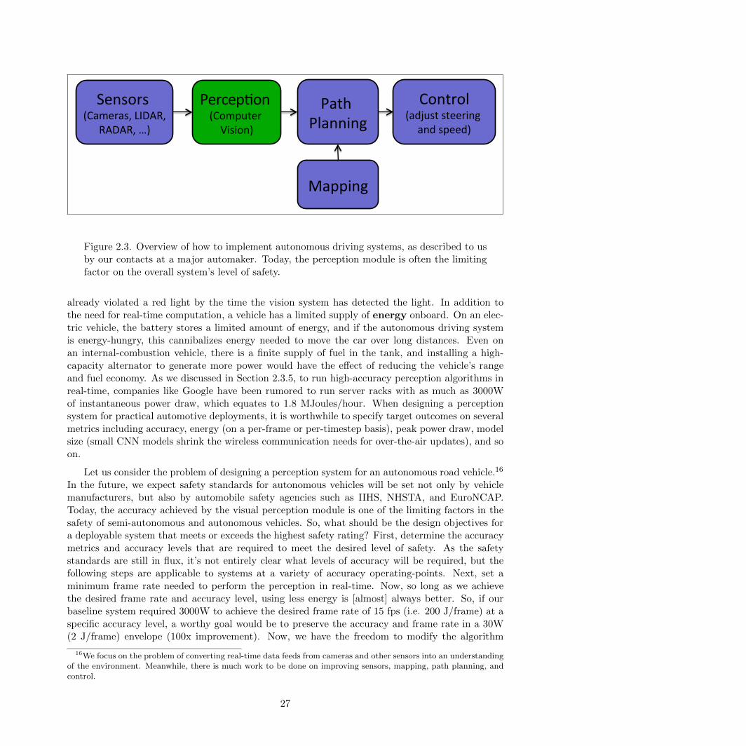
2"

DeepScale How$to$implement$autonomous$driving$

•  All"levels"of"vehicle"autonomy"(Level"1"–"Level"4)"require"the"above"flow"to"work"

•  Percep&on"is"o@en"the"weakest"link"(based"on"conversaBons"with"Tesla,"BMW,"and"others)"

•  Improving"the"accuracy"of"percepBon"will"lead"to"improved"safety"for"all"levels"of"autonomy"

PercepBon""(Computer"Vision)"

Sensors""(Cameras,"LIDAR,"

RADAR,"…)"

Path"Planning"

Control"(adjust"steering"

and"speed)"

Mapping"

Figure 2.3. Overview of how to implement autonomous driving systems, as described to usby our contacts at a major automaker. Today, the perception module is often the limitingfactor on the overall system’s level of safety.

already violated a red light by the time the vision system has detected the light. In addition tothe need for real-time computation, a vehicle has a limited supply of energy onboard. On an elec-tric vehicle, the battery stores a limited amount of energy, and if the autonomous driving systemis energy-hungry, this cannibalizes energy needed to move the car over long distances. Even onan internal-combustion vehicle, there is a finite supply of fuel in the tank, and installing a high-capacity alternator to generate more power would have the effect of reducing the vehicle’s rangeand fuel economy. As we discussed in Section 2.3.5, to run high-accuracy perception algorithms inreal-time, companies like Google have been rumored to run server racks with as much as 3000Wof instantaneous power draw, which equates to 1.8 MJoules/hour. When designing a perceptionsystem for practical automotive deployments, it is worthwhile to specify target outcomes on severalmetrics including accuracy, energy (on a per-frame or per-timestep basis), peak power draw, modelsize (small CNN models shrink the wireless communication needs for over-the-air updates), and soon.

Let us consider the problem of designing a perception system for an autonomous road vehicle.16

In the future, we expect safety standards for autonomous vehicles will be set not only by vehiclemanufacturers, but also by automobile safety agencies such as IIHS, NHSTA, and EuroNCAP.Today, the accuracy achieved by the visual perception module is one of the limiting factors in thesafety of semi-autonomous and autonomous vehicles. So, what should be the design objectives fora deployable system that meets or exceeds the highest safety rating? First, determine the accuracymetrics and accuracy levels that are required to meet the desired level of safety. As the safetystandards are still in flux, it’s not entirely clear what levels of accuracy will be required, but thefollowing steps are applicable to systems at a variety of accuracy operating-points. Next, set aminimum frame rate needed to perform the perception in real-time. Now, so long as we achievethe desired frame rate and accuracy level, using less energy is [almost] always better. So, if ourbaseline system required 3000W to achieve the desired frame rate of 15 fps (i.e. 200 J/frame) at aspecific accuracy level, a worthy goal would be to preserve the accuracy and frame rate in a 30W(2 J/frame) envelope (100x improvement). Now, we have the freedom to modify the algorithm

16We focus on the problem of converting real-time data feeds from cameras and other sensors into an understandingof the environment. Meanwhile, there is much work to be done on improving sensors, mapping, path planning, andcontrol.

27

(e.g. CNN architecture), software implementation, and choice of hardware, all to target improvedenergy-efficiency without compromising accuracy or frame rate. In other words: the metric ofenergy (J/frame) transcends the boundaries of algorithm, software, and hardware, so optimizingfor this metric promotes creativity and codesign of multiple layers of the system.

2.4.2 Per-component benchmarking

While the overall goal may be to reduce energy per frame (a system-level metric), let us considerthe dynamics of a team working toward this goal. In a typical case, the team would include at leastone hardware architect, at least one software architect, and at least one CNN architect. For allthree team members, the work may focus on identifying usable off-the-shelf solutions (e.g. existingCNN architectures, existing software libraries, and existing hardware components), or developingentirely new solutions (new CNN architectures, new software libraries, and new hardware), or —most likely — pursuing a mixture of off-the-shelf and custom solutions. Each team member willwant to evaluate his or her own contributions toward the common cause of improving energy-efficiency. We refer to this exercise as per-component benchmarking. The team can do this asfollows:

• The hardware architect can aim to maximize speed of a representative microbenchmark interms of OPS/sec. Further, the hardware architect can aim to minimize the power needed torun at peak OPS/sec. This power envelope should include not only the processor itself, butalso memory and I/O power requirements.

• The CNN architect has several ways to evaluate their work in isolation. Accuracy is a prop-erty of the CNN only, and not the software or hardware (assuming no bugs are introduced bynew software or hardware). Further, the quantity of computation (number of OPS per image;not per second) allows the CNN architect to chart their progress in reducing computationalrequirements. Model size is a metric that helps the CNN architect to understand the level ofthe memory hierarchy in which the model parameters may reside.

• The software architect has a more difficult time than the other two architects when at-tempting to isolate his/her contributions with per-component benchmarks. The softwarearchitect can aim to maximize speed (OPS/sec) of relevant CNN problem sizes on represen-tative hardware. If new hardware is being developed, some of this benchmarking may needto occur on simulation-based or FGPA-based prototypes of the proposed hardware. Ideally,the software architect can communicate frequently with the hardware architect and CNNarchitect, trading notes on hardware limitations and CNN problem dimensions that can beimplemented efficiently.

As we discussed in Sections 2.3.2 and 2.3.4, a software+hardware system does not always achievepeak OPS/sec on all problem sizes, so the software and hardware architects should be constantlyexchanging notes with the CNN architect on problem dimensions.

28

2.5 Relationship of our approach to the MESCAL methodology

The MESCAL book [34] points out that many new computer architectures are developed andevaluated using inadequate benchmarks that are not representative of the end applications. Espe-cially at the time when the MESCAL book was written, it was common to see new architecturesand chips evaluated based on the number of clock cycles needed to execute a series of instruc-tions. Ideally, the instruction stream would at least be derived from a motivating application (e.g.network packet processing), but sometimes these instructions are chosen more arbitrarily. Notsurprisingly, when application-specific processors are developed with such vague benchmarks andobjectives, these new processors don’t necessarily deliver improvements on end-application speedand efficiency.

As an antidote to this phenomenon, the MESCAL book advocates for system-level benchmark-ing. This type of benchmarking calls for representative algorithms, implementations, and inputswhen evaluating new hardware. Evaluating the top-to-bottom system on metrics such as speed,energy-efficiency, and correctness is the only sure-fire way to understand how the new hardwarewill perform on the end application.

In our discussion of benchmarks and metrics for evaluating deep learning systems, we haveadvocated for system-level benchmarking. This is well aligned with the MESCAL methodology.For example, the speed (i.e. frame rate during training or inference) of a CNN/DNN system isinfluenced by all levels of the stack, including the dimensionality of the input data, the neuralarchitecture, the software, and the hardware. Likewise, the energy per frame is influenced by all ofthese factors. These metrics — and how these can be traded off with accuracy — are system-levelbenchmarks that promote co-design of all levels of the stack to develop the best possible system.

While system-level benchmarking is the most vital type of benchmarking, we find that thereare cases where per-component benchmarks are useful, too. For example, the accuracy of theCNN/DNN model is independent of the software and hardware in which it is implemented17, sothe model’s accuracy can be analyzed independently of the rest of the system. Likewise, the numberof arithmetic operations in a CNN is a property of the CNN alone. Further, the peak power envelopeis purely a property of the hardware. These per-component metrics are useful for individual teamsin an organization (e.g. the CNN team, the software team, and the hardware team) to evaluatetheir individual contributions. However, the “north star” or guiding light should always be thesystem-level metrics that represent the end-application behavior.

17If the CNN’s accuracy changes when moving to a different software implementation or hardware platform, thisis considered a bug. However, there are opportunities for co-design, such as leveraging hardware that can efficientlydo CNN computations at low precision, and then working to mitigate the possible drop in accuracy.

29

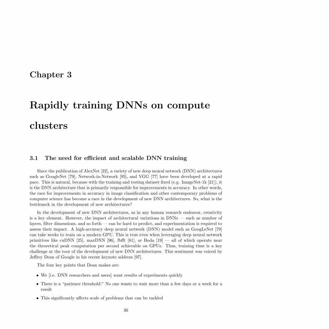
Chapter 3

Rapidly training DNNs on compute

clusters

3.1 The need for efficient and scalable DNN training

Since the publication of AlexNet [22], a variety of new deep neural network (DNN) architecturessuch as GoogleNet [79], Network-in-Network [95], and VGG [77] have been developed at a rapidpace. This is natural, because with the training and testing dataset fixed (e.g. ImageNet-1k [21]), itis the DNN architecture that is primarily responsible for improvements in accuracy. In other words,the race for improvements in accuracy in image classification and other contemporary problems ofcomputer science has become a race in the development of new DNN architectures. So, what is thebottleneck in the development of new architectures?

In the development of new DNN architectures, as in any human research endeavor, creativityis a key element. However, the impact of architectural variations in DNNs — such as number oflayers, filter dimensions, and so forth — can be hard to predict, and experimentation is required toassess their impact. A high-accuracy deep neural network (DNN) model such as GoogLeNet [79]can take weeks to train on a modern GPU. This is true even when leveraging deep neural networkprimitives like cuDNN [25], maxDNN [96], fbfft [81], or Boda [19] — all of which operate nearthe theoretical peak computation per second achievable on GPUs. Thus, training time is a keychallenge at the root of the development of new DNN architectures. This sentiment was voiced byJeffrey Dean of Google in his recent keynote address [97].

The four key points that Dean makes are:

• We [i.e. DNN researchers and users] want results of experiments quickly

• There is a “patience threshold:” No one wants to wait more than a few days or a week for aresult

• This significantly affects scale of problems that can be tackled

30

• We sometimes optimize for experiment turnaround time, rather than absolute minimal systemresources for performing the experiment

Given the considerable resources available to Google researchers, Dean’s comments indicatethat simply throwing more computational resources at the problem is not sufficient to solve theDNN training problem. In the following, we will spend a little more time dimensionalizing thecurrent problems with DNN training and the upside potential if these problems can be solved.

3.1.1 Accelerating DNN Research and Development

As a particular example of where long training times are limiting the pace of DNN research andproductization, consider the following. ImageNet-1k has 1.2 million training images, distributedacross 1000 different category labels. From first-hand conversations with engineers and executives,we know that several internet companies have internal databases containing billions of images withhundreds of thousands of different category labels. Due to long training times, these companiesare facing serious delays in bringing DNN-based solutions to market. Accelerated DNN trainingsolutions would address a major pain point for these companies.

3.1.2 Real-Time DNN Training

So far, we have argued how accelerating DNN training would benefit applications where DNNsare in use today. Now, we consider ways in which accelerating DNN training would allow DNN-based techniques to be applied in entirely new ways. There are a number of situations where itis crucial to incorporate new data into a DNN model in real time. For example, reinforcementlearning (RL) enables robots to learn things themselves with minimal supervision. A recent studyby Levine et al. applied state-of-the-art DNN-based RL techniques to enable a robot to teach itselfhow to build lego structures and screw on bottle caps [98]. This technique is effective, and therobot does indeed learn to screw on bottle caps. However, it takes 3-4 hours for the robot to learnto screw on bottle caps, and the majority of this time is spent on DNN training. Faster DNNtraining would enable this and other reinforcement learning applications to move toward real-time.

Deep Neural Networks are used for an ever-broadening variety of problems, including classify-ing [79, 55] and detecting [47, 48] objects in images, writing sentences about images [57], identifyingactions in videos [12], performing speech recognition [99], and gaining semantic understanding oftext [10]. We anticipate that sophisticated reinforcement learning (RL) systems in robotics willeventually leverage all of these modalities, ideally in real-time.

3.1.3 Accelerating DNN Training with FireCaffe

In our work, we focus directly on the problem of DNN training. Since single-GPU efficiency hasreached the hard limits of the hardware, the next frontier for accelerating DNN training is to scaleit across a compute cluster. In this chapter, we present FireCaffe, which scales DNN training acrossa cluster of 128 GPUs with speedups of more than 40x compared to a single GPU. Our strategy forscaling up DNN training is to focus on reducing communication overhead, and we make a numberof design choices toward this goal. For example, we use fast interconnects such as Infiniband or

31

Cray Gemini to accelerate communication among the GPUs. We also show that reduction treesare a faster method for communication than using parameter servers. We map our parallelizationstrategy to high-accuracy DNN architectures that require less communication.

The rest of this chapter is organized as follows. In Section 3.2, we describe our choice ofhardware for evaluating scalable DNN training, and Section 3.3 introduces key factors that wewill use for analyzing communication among GPU workers. We describe tradeoffs between DNNparallelism strategies in Section 3.4, and Section 3.5 explains why certain high-accuracy DNNarchitectures are particularly amenable to parallelism. In Section 3.6, we describe our approachto efficiently implementing distributed DNN training. In Section 3.7, we describe good practicesthat facilitate the comparison of scalable DNN training techniques and we present our speedups fortraining the NiN and GoogLeNet architectures on ImageNet. Section 3.8 describes approaches thatare complimentary to FireCaffe for further accelerating DNN training. We conclude in Section 3.9.

3.2 Hardware for scalable DNN training

It is both useful and feasible to experiment with the scalability of DNN computations usingtheoretical or scale models. However, demonstration and verification of the correctness and real-world scalability of the proposed FireCaffe system requires using concrete hardware platforms.The speed at which data can be sent between nodes is a key consideration in selecting a hardwareplatform for scalable DNN training. This is because, the faster the interconnect between nodes is,the more scale we can achieve without being dominated by communication overhead. Hardwaremanufacturers such as Cray and Mellanox address this by developing high-bandwidth, low-latencyinterconnects that are substantially faster than typical Ethernet connections.

For example, the Titan supercomputer at Oak Ridge Leadership Computing Facility (OLCF)has a high bandwidth, low latency Cray Gemini interconnect for communication among servers.The Titan supercomputer has a total of 18,000 servers, with one NVIDIA Kepler-based K20x GPUper server [100, 101]. With this in mind, we choose the OLCF Titan supercomputer for tuning andevaluating FireCaffe.

In this research, we use relatively small slices of the overall capacity of Titan for each trainingrun. The additional computational capacity (∼27 PetaFLOPS/s in total) enables us to conductmultiple training runs concurrently, where each training run utilizes 32 to 128 GPUs. When con-sidering 32-node slices of Titan, we found that the interconnect speed (at least for the applicationsof this work) is similar to that provided by having all nodes in the slice connected to a singleInfiniband-class switch.

3.3 Preliminaries and terminology

To minimize confusion, we now define some terminology. The key data structures in a convo-lution layer are data (also called activations) and parameters (also called weights), and we presenta simple illustration of this in Figure 3.1.1 More explicitly: in our terminology, the each of thefollowing sets of words are synonyms: (weights = parameters = filters = W ); (nodes = workers

1For a much more detailed discussion of how convolution layers work, see Section 4.2.1.

32

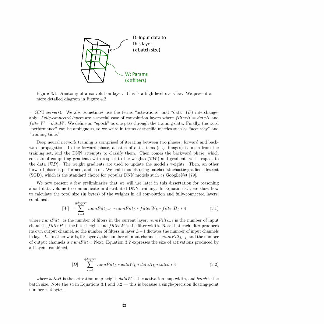
W:#Params#(x##filters)#

D:#Input#data#to#this#layer#(x#batch#size)#

Figure 3.1. Anatomy of a convolution layer. This is a high-level overview. We present amore detailed diagram in Figure 4.2.

= GPU servers). We also sometimes use the terms “activations” and “data” (D) interchange-ably. Fully-connected layers are a special case of convolution layers where filterH = dataH andfilterW = dataW . We define an “epoch” as one pass through the training data. Finally, the word“performance” can be ambiguous, so we write in terms of specific metrics such as “accuracy” and“training time.”

Deep neural network training is comprised of iterating between two phases: forward and back-ward propagation. In the forward phase, a batch of data items (e.g. images) is taken from thetraining set, and the DNN attempts to classify them. Then comes the backward phase, whichconsists of computing gradients with respect to the weights (∇W ) and gradients with respect tothe data (∇D). The weight gradients are used to update the model’s weights. Then, an otherforward phase is performed, and so on. We train models using batched stochastic gradient descent(SGD), which is the standard choice for popular DNN models such as GoogLeNet [79].

We now present a few preliminaries that we will use later in this dissertation for reasoningabout data volume to communicate in distributed DNN training. In Equation 3.1, we show howto calculate the total size (in bytes) of the weights in all convolution and fully-connected layers,combined.

|W | =#layers∑L=1

numFiltL−1 ∗ numFiltL ∗ filterWL ∗ filterHL ∗ 4 (3.1)

where numFiltL is the number of filters in the current layer, numFiltL−1 is the number of inputchannels, filterH is the filter height, and filterW is the filter width. Note that each filter producesits own output channel, so the number of filters in layer L−1 dictates the number of input channelsin layer L. In other words, for layer L, the number of input channels is numFiltL−1, and the numberof output channels is numFiltL. Next, Equation 3.2 expresses the size of activations produced byall layers, combined.

|D| =#layers∑L=1

numFiltL ∗ dataWL ∗ dataHL ∗ batch ∗ 4 (3.2)

where dataH is the activation map height, dataW is the activation map width, and batch is thebatch size. Note the ∗4 in Equations 3.1 and 3.2 — this is because a single-precision floating-pointnumber is 4 bytes.

33

3.4 Parallelism strategies

There are two commonly-used methods for parallelizing neural network training across multipleservers: model parallelism (e.g. [102]) and data parallelism (e.g. [103]).

For batched SGD training of DNNs, we define data parallelism as the case where each worker(e.g. GPU) gets a subset of the batch, and then the workers communicate by exchanging weightgradient updates ∇W . We define model parallelism as the case where each worker gets a subsetof the model parameters, and the workers communicate by exchanging data gradients ∇D andexchanging activations D. Note that |W | = |∇W | and |D| = |∇D|; in other words, the weightsand weight gradients are the same size; and the data and data gradients are the same size.

Now, to maximize DNN training scalability, our goal is to select a parallelism strategy thatrequires the lowest possible quantity of communication between servers. The choice of whetherit is ideal to use data parallelism, model parallelism, or both depends strongly on the DNN’sarchitectural characteristics. Commonly-used DNN architectures for speech recognition (e.g. [104])consist primarily of fully-connected layers, where the activations and parameters have the samespatial resolution (typically 1x1). For typical batch sizes, these fully-connected models often havea similar quantity of weights W and activations D. For example, we observe in Table 3.1 that thisproperty holds true for the MSFT-Speech DNN architecture [104].

In computer vision, some of the most popular and accurate DNN models (e.g. GoogLeNet [79])consist primarily of convolution layers, where the spatial resolution of the filters is smaller thanthe resolution of the activations.2 For these convolutional models, data parallelism is typicallypreferable because it requires less communication — that is, |∇W | is much smaller than |∇D| attypical batch sizes. Notice that the computer vision DNNs in Table 3.1 all have this property. InFireCaffe, we enable data parallelism across a cluster of GPUs, and we find that it produces amplespeedups for training popular deep convolutional neural network architectures. We illustrate ourdata parallel approach in Figure 3.2. In this configuration, all the GPUs contain the full DNNmodel parameters. Each worker (GPU) gets a subset of each batch. The GPUs compute theirshare of the weight gradients. Once the gradients are calculated locally, they are added togetherusing either a parameter server or a reduction tree communication (described in Section 3.6.2).

2For a more detailed discussion of the dimensionality of parameters and activations, skip ahead to Section 4.3.

34

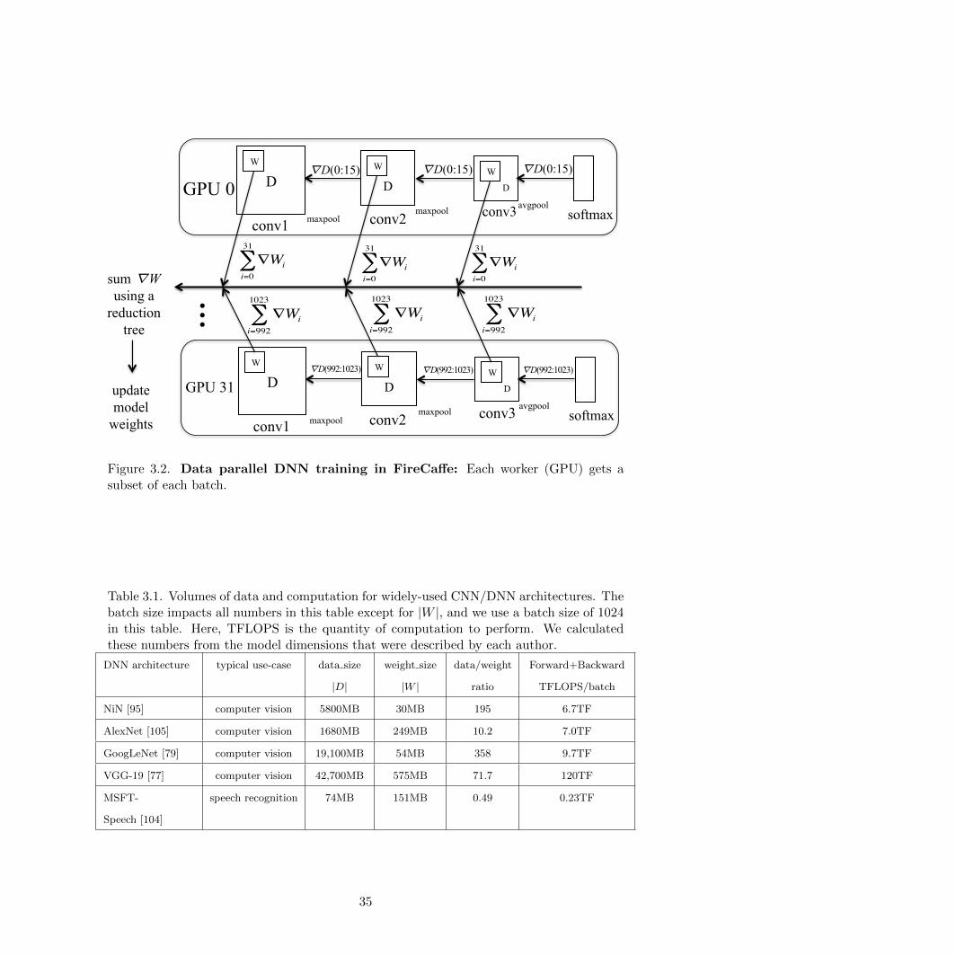
conv1 conv2 conv3 softmax

sum �W using a

reduction tree

update model

weights

�D(0:15)

GPU 0 …

D

W D

W D

W

maxpool maxpool avgpool

�D(0:15) �D(0:15)

∇Wii=0

31

∑

conv1 conv2 conv3 softmax

�D(992:1023)

GPU 31 D W

D

W D

W

maxpool maxpool avgpool

∇Wii=992

1023

∑

∇Wii=0

31

∑ ∇Wii=0

31

∑

∇Wii=992

1023

∑ ∇Wii=992

1023

∑

�D(992:1023) �D(992:1023)

Figure 3.2. Data parallel DNN training in FireCaffe: Each worker (GPU) gets asubset of each batch.

Table 3.1. Volumes of data and computation for widely-used CNN/DNN architectures. Thebatch size impacts all numbers in this table except for |W |, and we use a batch size of 1024in this table. Here, TFLOPS is the quantity of computation to perform. We calculatedthese numbers from the model dimensions that were described by each author.

DNN architecture typical use-case data size

|D|

weight size

|W |

data/weight

ratio

Forward+Backward

TFLOPS/batch

NiN [95] computer vision 5800MB 30MB 195 6.7TF

AlexNet [105] computer vision 1680MB 249MB 10.2 7.0TF

GoogLeNet [79] computer vision 19,100MB 54MB 358 9.7TF

VGG-19 [77] computer vision 42,700MB 575MB 71.7 120TF

MSFT-

Speech [104]

speech recognition 74MB 151MB 0.49 0.23TF

35

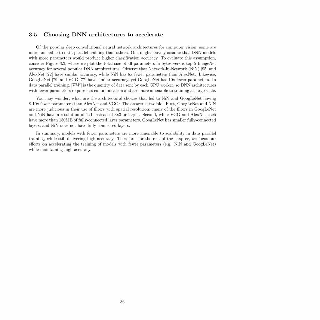
3.5 Choosing DNN architectures to accelerate

Of the popular deep convolutional neural network architectures for computer vision, some aremore amenable to data parallel training than others. One might naıvely assume that DNN modelswith more parameters would produce higher classification accuracy. To evaluate this assumption,consider Figure 3.3, where we plot the total size of all parameters in bytes versus top-5 ImageNetaccuracy for several popular DNN architectures. Observe that Network-in-Network (NiN) [95] andAlexNet [22] have similar accuracy, while NiN has 8x fewer parameters than AlexNet. Likewise,GoogLeNet [79] and VGG [77] have similar accuracy, yet GoogLeNet has 10x fewer parameters. Indata parallel training, |∇W | is the quantity of data sent by each GPU worker, so DNN architectureswith fewer parameters require less communication and are more amenable to training at large scale.

You may wonder, what are the architectural choices that led to NiN and GoogLeNet having8-10x fewer parameters than AlexNet and VGG? The answer is twofold. First, GoogLeNet and NiNare more judicious in their use of filters with spatial resolution: many of the filters in GoogLeNetand NiN have a resolution of 1x1 instead of 3x3 or larger. Second, while VGG and AlexNet eachhave more than 150MB of fully-connected layer parameters, GoogLeNet has smaller fully-connectedlayers, and NiN does not have fully-connected layers.

In summary, models with fewer parameters are more amenable to scalability in data paralleltraining, while still delivering high accuracy. Therefore, for the rest of the chapter, we focus ourefforts on accelerating the training of models with fewer parameters (e.g. NiN and GoogLeNet)while maintaining high accuracy.

36

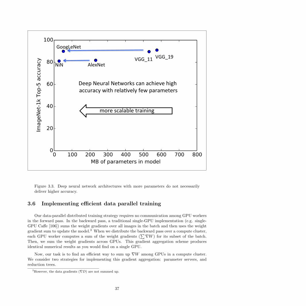
AlexNet'

Deep'Neural'Networks'can'achieve'high'accuracy'with'rela8vely'few'parameters'

more'scalable'training'

GoogLeNet'

NiN'VGG_11' VGG_19'

Figure 3.3. Deep neural network architectures with more parameters do not necessarilydeliver higher accuracy.

3.6 Implementing efficient data parallel training

Our data-parallel distributed training strategy requires no communication among GPU workersin the forward pass. In the backward pass, a traditional single-GPU implementation (e.g. single-GPU Caffe [106]) sums the weight gradients over all images in the batch and then uses the weightgradient sum to update the model.3 When we distribute the backward pass over a compute cluster,each GPU worker computes a sum of the weight gradients (

∑∇W ) for its subset of the batch.Then, we sum the weight gradients across GPUs. This gradient aggregation scheme producesidentical numerical results as you would find on a single GPU.

Now, our task is to find an efficient way to sum up ∇W among GPUs in a compute cluster.We consider two strategies for implementing this gradient aggregation: parameter servers, andreduction trees.

3However, the data gradients (∇D) are not summed up.

37

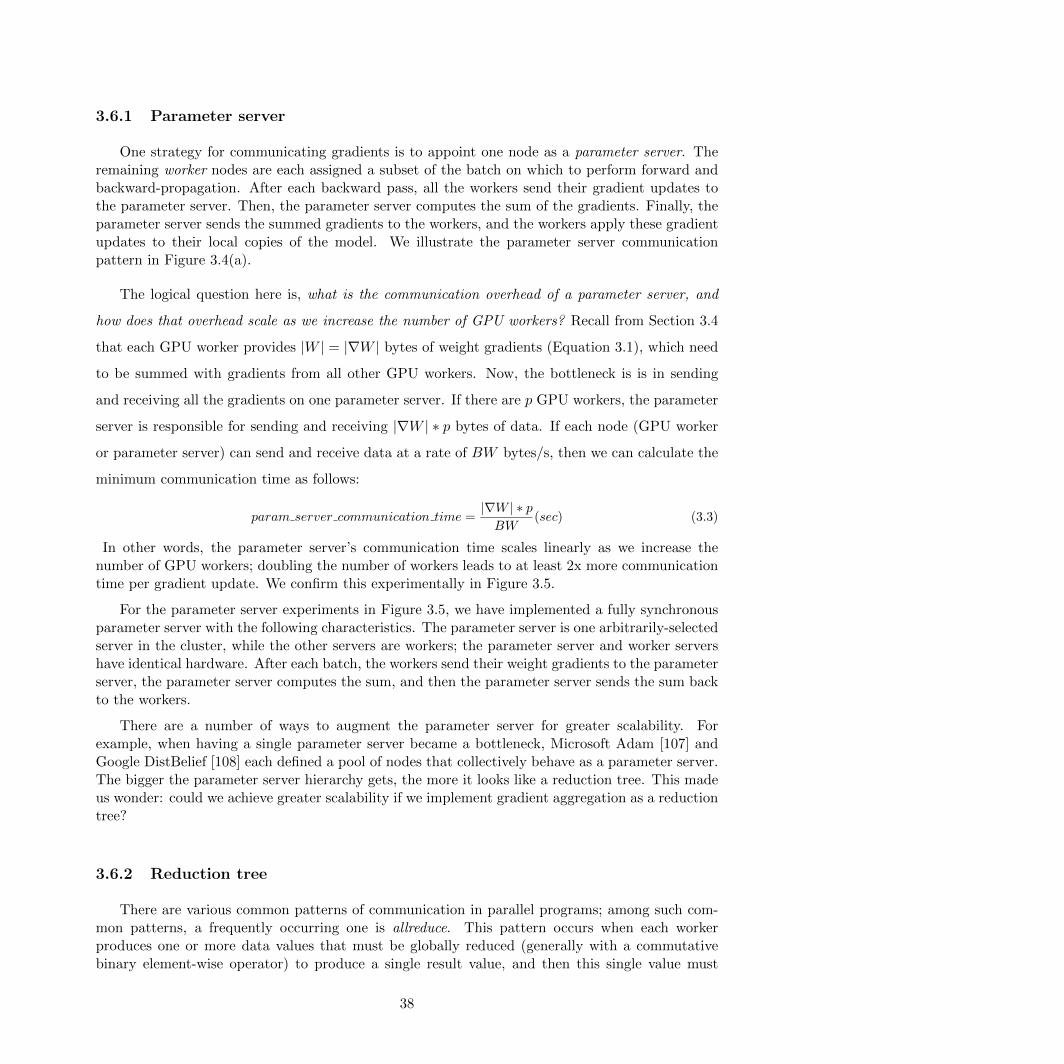
3.6.1 Parameter server

One strategy for communicating gradients is to appoint one node as a parameter server. Theremaining worker nodes are each assigned a subset of the batch on which to perform forward andbackward-propagation. After each backward pass, all the workers send their gradient updates tothe parameter server. Then, the parameter server computes the sum of the gradients. Finally, theparameter server sends the summed gradients to the workers, and the workers apply these gradientupdates to their local copies of the model. We illustrate the parameter server communicationpattern in Figure 3.4(a).

The logical question here is, what is the communication overhead of a parameter server, and

how does that overhead scale as we increase the number of GPU workers? Recall from Section 3.4

that each GPU worker provides |W | = |∇W | bytes of weight gradients (Equation 3.1), which need

to be summed with gradients from all other GPU workers. Now, the bottleneck is is in sending

and receiving all the gradients on one parameter server. If there are p GPU workers, the parameter

server is responsible for sending and receiving |∇W | ∗ p bytes of data. If each node (GPU worker

or parameter server) can send and receive data at a rate of BW bytes/s, then we can calculate the

minimum communication time as follows:

param server communication time =|∇W | ∗ p

BW(sec) (3.3)

In other words, the parameter server’s communication time scales linearly as we increase thenumber of GPU workers; doubling the number of workers leads to at least 2x more communicationtime per gradient update. We confirm this experimentally in Figure 3.5.

For the parameter server experiments in Figure 3.5, we have implemented a fully synchronousparameter server with the following characteristics. The parameter server is one arbitrarily-selectedserver in the cluster, while the other servers are workers; the parameter server and worker servershave identical hardware. After each batch, the workers send their weight gradients to the parameterserver, the parameter server computes the sum, and then the parameter server sends the sum backto the workers.

There are a number of ways to augment the parameter server for greater scalability. Forexample, when having a single parameter server became a bottleneck, Microsoft Adam [107] andGoogle DistBelief [108] each defined a pool of nodes that collectively behave as a parameter server.The bigger the parameter server hierarchy gets, the more it looks like a reduction tree. This madeus wonder: could we achieve greater scalability if we implement gradient aggregation as a reductiontree?

3.6.2 Reduction tree

There are various common patterns of communication in parallel programs; among such com-mon patterns, a frequently occurring one is allreduce. This pattern occurs when each workerproduces one or more data values that must be globally reduced (generally with a commutativebinary element-wise operator) to produce a single result value, and then this single value must

38

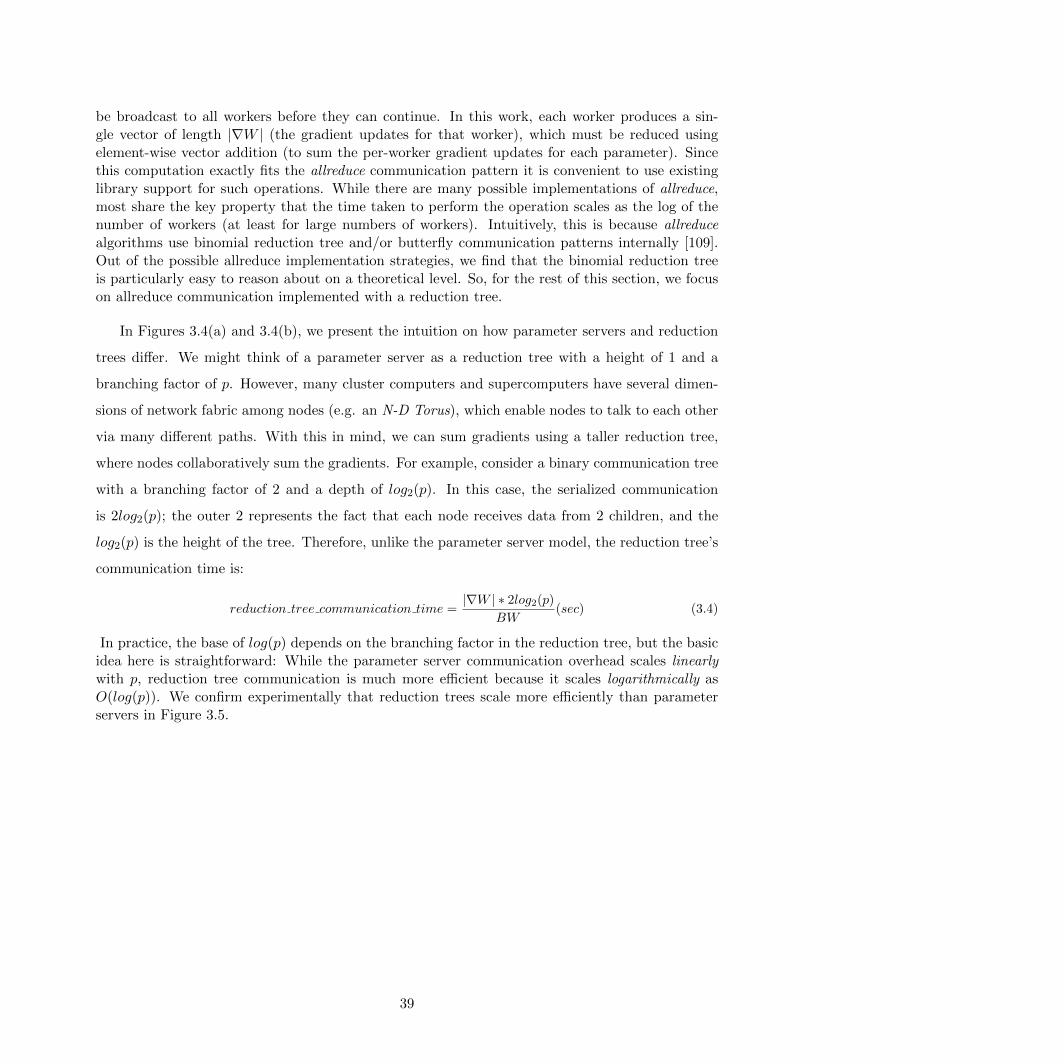
be broadcast to all workers before they can continue. In this work, each worker produces a sin-gle vector of length |∇W | (the gradient updates for that worker), which must be reduced usingelement-wise vector addition (to sum the per-worker gradient updates for each parameter). Sincethis computation exactly fits the allreduce communication pattern it is convenient to use existinglibrary support for such operations. While there are many possible implementations of allreduce,most share the key property that the time taken to perform the operation scales as the log of thenumber of workers (at least for large numbers of workers). Intuitively, this is because allreducealgorithms use binomial reduction tree and/or butterfly communication patterns internally [109].Out of the possible allreduce implementation strategies, we find that the binomial reduction treeis particularly easy to reason about on a theoretical level. So, for the rest of this section, we focuson allreduce communication implemented with a reduction tree.

In Figures 3.4(a) and 3.4(b), we present the intuition on how parameter servers and reduction

trees differ. We might think of a parameter server as a reduction tree with a height of 1 and a

branching factor of p. However, many cluster computers and supercomputers have several dimen-

sions of network fabric among nodes (e.g. an N-D Torus), which enable nodes to talk to each other

via many different paths. With this in mind, we can sum gradients using a taller reduction tree,

where nodes collaboratively sum the gradients. For example, consider a binary communication tree

with a branching factor of 2 and a depth of log2(p). In this case, the serialized communication

is 2log2(p); the outer 2 represents the fact that each node receives data from 2 children, and the

log2(p) is the height of the tree. Therefore, unlike the parameter server model, the reduction tree’s

communication time is:

reduction tree communication time =|∇W | ∗ 2log2(p)

BW(sec) (3.4)

In practice, the base of log(p) depends on the branching factor in the reduction tree, but the basicidea here is straightforward: While the parameter server communication overhead scales linearlywith p, reduction tree communication is much more efficient because it scales logarithmically asO(log(p)). We confirm experimentally that reduction trees scale more efficiently than parameterservers in Figure 3.5.

39

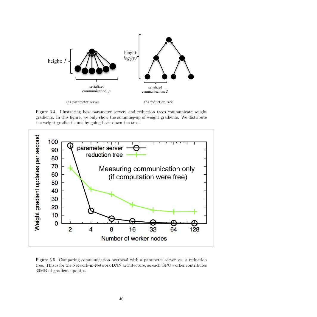
height: log2(p) height: 1

serialized communication: 2

serialized communication: p

(a) parameter server

height: log2(p) height: 1

serialized communication: 2

serialized communication: p

(b) reduction tree

Figure 3.4. Illustrating how parameter servers and reduction trees communicate weightgradients. In this figure, we only show the summing-up of weight gradients. We distributethe weight gradient sums by going back down the tree.

Measuring communication only (if computation were free)

Figure 3.5. Comparing communication overhead with a parameter server vs. a reductiontree. This is for the Network-in-Network DNN architecture, so each GPU worker contributes30MB of gradient updates.

40

3.7 Evaluation of FireCaffe-accelerated training on ImageNet

In this section, we evaluate how FireCaffe can accelerate DNN training on a cluster of GPUs.We train GoogLeNet [79] and Network-in-Network [95] on up to 128 GPU servers in the Titansupercomputer (described in Section 3.2), leveraging FireCaffe’s reduction tree data parallelism(Section 3.6.2). We begin by describing our evaluation methodology, and then we analyze theresults.

3.7.1 Evaluation Methodology

We now describe a few practices that aid in comparing advancements in accelerating thetraining of deep neural networks.

1. Evaluate the speed and accuracy of DNN training on a publicly-available dataset.In a recent study, Azizpour et al. applied DNNs to more than 10 different visual recognitionchallenge datasets, including human attribute prediction, fine-grained flower classification, andindoor scene recognition [110]. The accuracy obtained by Azizpour et al. ranged from 56% onscene recognition to 91% on human attribute prediction. As you can see, the accuracy of DNNsand other machine learning algorithms depends highly on the specifics of the application anddataset to which they are applied. Thus, when researchers report improvements in training speedor accuracy on proprietary datasets, there is no clear way to compare the improvements withthe related literature. For example, Baidu [111] and Amazon [112] recently presented results onaccelerating DNN training. Amazon and Baidu4 each reported their training time numbers ona proprietary dataset, so it’s not clear how to compare these results with the related literature.In contrast, we conduct our evaluation on a publicly-available dataset, ImageNet-1k [21], whichcontains more than 1 million training images, and each image is labeled as containing 1 of 1000object categories. ImageNet-1k is a widely-studied dataset, so we can easily compare our accuracy,training speed, and scalability results with other studies that use this data.

2. Report hyperparameter settings such as weight initialization, momentum, batchsize, and learning rate.Glorot et al. [113], Breuel [114], and Xu et al. [115] have each shown that seemingly-subtlehyperparameter settings such as weight initialization can have a big impact on the speed andaccuracy produced in DNN training. When training Network-in-Network (NiN) [95], we initializethe weights with a Gaussian distribution centered at 0, and we set the standard deviation (std) to0.01 for 1x1 convolution layers, and we use std=0.05 for other layers. For NiN, we initialize the biasterms to a constant value of 0, we set the weight decay to 0.0005, and we set momentum to 0.9.These settings are derived from with the Caffe configuration files released by the NiN authors [95].

Frustratingly, in Google’s technical reports on GoogLeNet [79, 116], training details such asbatch size, momentum, and learning rate are not disclosed. Fortunately, Wu et al. [117] andGuadarrama [61] each reproduced GoogLeNet and released all the details of their training protocols.As in [61], we train GoogLeNet with momentum=0.9 and weight decay=0.0002, we use xavier [113]

4Baidu evaluated their training times using proprietary dataset [111]. Baidu also did some ImageNet experiments,but Baidu did not report the training time on ImageNet.

41

weight initialization, and we initialize the bias terms to a constant value of 0.2. We will addresslearning rate and batch size settings in the following sections.

Given a DNN architecture, there are a number of strategies that can further increase accuracy,albeit at a substantial computational cost. One such strategy is to train multiple independentcopies of a DNN architecture (e.g. GoogLeNet), each with a different random number generatorseed for initializing the parameters. At test time, these DNNs can be used as an ensemble —that is, all DNNs are run on the test data, and for each test data item, the DNN’s classifica-tion activations are averaged. For example, using an ensemble of 7 GoogLeNet DNNs, Szegedyet al. achieved a 2 percentage-point accuracy improvement on ImageNet, compared to a singleGoogLeNet baseline [79]. An other such technique is to augment the data by adding deformationsor color variations during training and/or testing [111]. Our focus in this chapter is to showspeedup on training single models and compare with reported baselines. Hence we avoid usingexotic data augmentation or ensembles of multiple DNNs. In our experiments, we resize imagesto 256x256; at training time we use a 224x224 crop with a randomized offset, and at test time weclassify the 224x224 crop in the center of the image; these settings are also commonly used in theAlexNet [22] and Network-in-Network [95] DNN architectures.

3. Measure speedups with respect to a single-server baseline.In order to meaningfully measure how much we have accelerated DNN training by adding moreGPUs, we must have a representative baseline, e.g. with a single GPU. When reporting results, webegin by considering time required to train a DNN on single GPU, and we report our multi-GPUspeedups with respect to this single-GPU baseline. A recent study by Microsoft [107] reportedtraining a custom DNN architecture (e.g. not GoogLeNet or NiN) on a cluster of CPU servers.This may sound impressive, but Microsoft did not report the time that the model would take totrain on a single server. It could be that Microsoft achieved a 10x speedup by going from 1 serverto 10 servers, or the speedup could be 2x — this isn’t clear from the information provided inMicrosoft’s paper. This illustrates the importance of measuring the speed of scalable DNN trainingsystems with respect to a single-server baseline.

4. Measure accuracy with respect to a single-server baseline.In our experience, if hyperparameters such as learning rate and batch size are selected too aggres-sively, a DNN model may converge quickly, but fall short of the state-of-art accuracy. Therefore,in our experiments, we train multi-GPU models until they reach to the single-GPU accuracy base-line; this validates that we can accelerate DNN training without degrading accuracy. However,in cluster-scale multi-GPU training experiments by Baidu [111] and Flickr [118], the training isstopped prematurely before the DNNs converge. This leaves us wondering whether the Baidu andFlickr multi-GPU training experiments would have reproduced the accuracy produced on a singleGPU. To avoid this type of confusion, we evaluate both the speed and accuracy of FireCaffe DNNtraining with respect to a single-server/single-GPU baseline.

3.7.2 Results: Midsized deep models

Using the settings described by Krizhevsky [22], we find that AlexNet achieves 58.9% top-1ImageNet-1k accuracy after 100 epochs of training. After just 47 epochs of training, we find thatNiN also converges to 58.9% top-1 accuracy. Each training iteration of NiN is more time-consuming

42

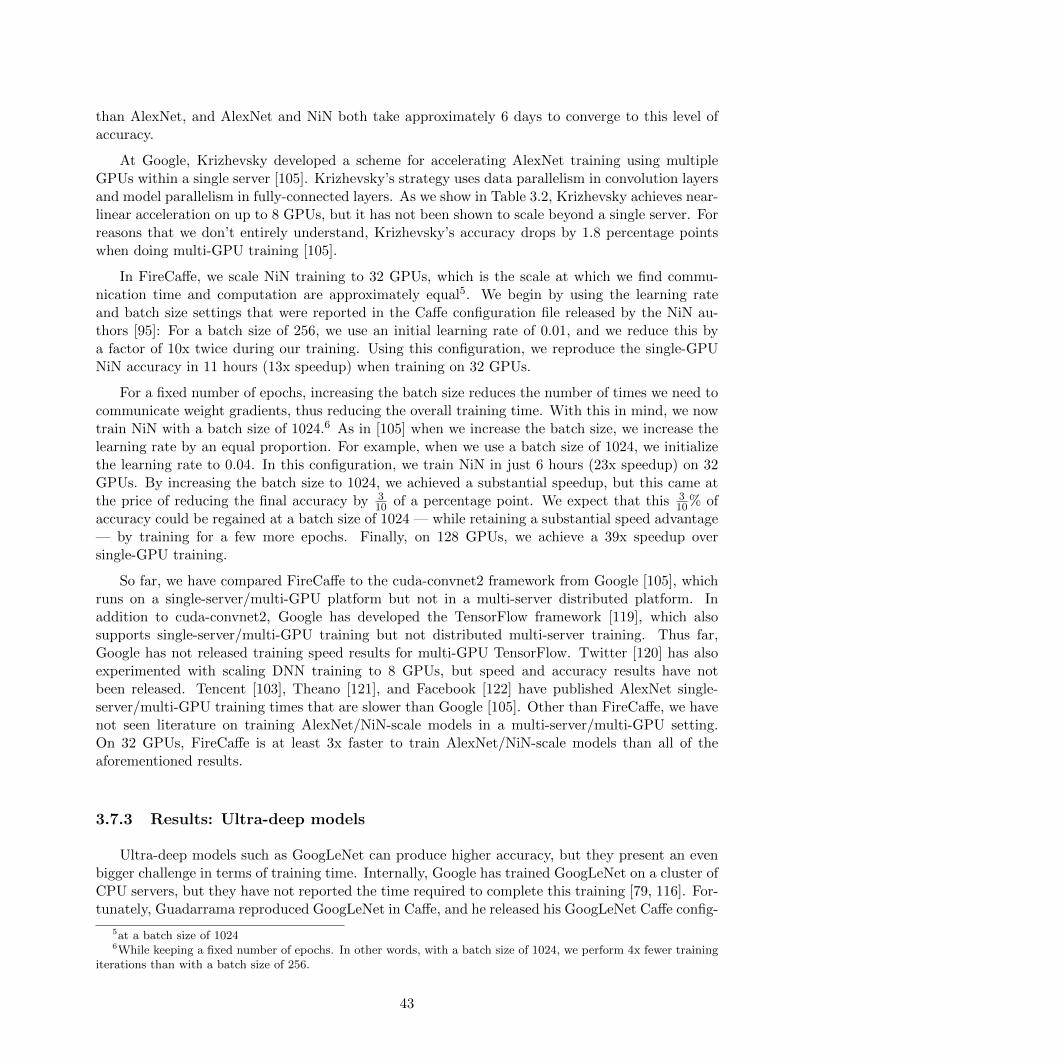
than AlexNet, and AlexNet and NiN both take approximately 6 days to converge to this level ofaccuracy.

At Google, Krizhevsky developed a scheme for accelerating AlexNet training using multipleGPUs within a single server [105]. Krizhevsky’s strategy uses data parallelism in convolution layersand model parallelism in fully-connected layers. As we show in Table 3.2, Krizhevsky achieves near-linear acceleration on up to 8 GPUs, but it has not been shown to scale beyond a single server. Forreasons that we don’t entirely understand, Krizhevsky’s accuracy drops by 1.8 percentage pointswhen doing multi-GPU training [105].

In FireCaffe, we scale NiN training to 32 GPUs, which is the scale at which we find commu-nication time and computation are approximately equal5. We begin by using the learning rateand batch size settings that were reported in the Caffe configuration file released by the NiN au-thors [95]: For a batch size of 256, we use an initial learning rate of 0.01, and we reduce this bya factor of 10x twice during our training. Using this configuration, we reproduce the single-GPUNiN accuracy in 11 hours (13x speedup) when training on 32 GPUs.

For a fixed number of epochs, increasing the batch size reduces the number of times we need tocommunicate weight gradients, thus reducing the overall training time. With this in mind, we nowtrain NiN with a batch size of 1024.6 As in [105] when we increase the batch size, we increase thelearning rate by an equal proportion. For example, when we use a batch size of 1024, we initializethe learning rate to 0.04. In this configuration, we train NiN in just 6 hours (23x speedup) on 32GPUs. By increasing the batch size to 1024, we achieved a substantial speedup, but this came atthe price of reducing the final accuracy by 3

10 of a percentage point. We expect that this 310% of

accuracy could be regained at a batch size of 1024 — while retaining a substantial speed advantage— by training for a few more epochs. Finally, on 128 GPUs, we achieve a 39x speedup oversingle-GPU training.

So far, we have compared FireCaffe to the cuda-convnet2 framework from Google [105], whichruns on a single-server/multi-GPU platform but not in a multi-server distributed platform. Inaddition to cuda-convnet2, Google has developed the TensorFlow framework [119], which alsosupports single-server/multi-GPU training but not distributed multi-server training. Thus far,Google has not released training speed results for multi-GPU TensorFlow. Twitter [120] has alsoexperimented with scaling DNN training to 8 GPUs, but speed and accuracy results have notbeen released. Tencent [103], Theano [121], and Facebook [122] have published AlexNet single-server/multi-GPU training times that are slower than Google [105]. Other than FireCaffe, we havenot seen literature on training AlexNet/NiN-scale models in a multi-server/multi-GPU setting.On 32 GPUs, FireCaffe is at least 3x faster to train AlexNet/NiN-scale models than all of theaforementioned results.

3.7.3 Results: Ultra-deep models

Ultra-deep models such as GoogLeNet can produce higher accuracy, but they present an evenbigger challenge in terms of training time. Internally, Google has trained GoogLeNet on a cluster ofCPU servers, but they have not reported the time required to complete this training [79, 116]. For-tunately, Guadarrama reproduced GoogLeNet in Caffe, and he released his GoogLeNet Caffe config-

5at a batch size of 10246While keeping a fixed number of epochs. In other words, with a batch size of 1024, we perform 4x fewer training

iterations than with a batch size of 256.

43

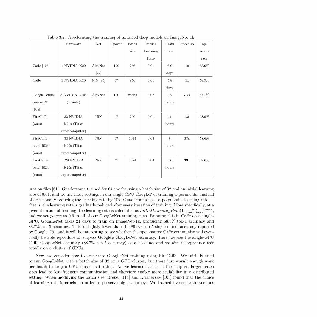
Table 3.2. Accelerating the training of midsized deep models on ImageNet-1k.

Hardware Net Epochs Batch

size

Initial

Learning

Rate

Train

time

Speedup Top-1

Accu-

racy

Caffe [106] 1 NVIDIA K20 AlexNet

[22]

100 256 0.01 6.0

days

1x 58.9%

Caffe 1 NVIDIA K20 NiN [95] 47 256 0.01 5.8

days

1x 58.9%

Google cuda-

convnet2

[105]

8 NVIDIA K20s

(1 node)

AlexNet 100 varies 0.02 16

hours

7.7x 57.1%

FireCaffe

(ours)

32 NVIDIA

K20s (Titan

supercomputer)

NiN 47 256 0.01 11

hours

13x 58.9%

FireCaffe-

batch1024

(ours)

32 NVIDIA

K20s (Titan

supercomputer)

NiN 47 1024 0.04 6

hours

23x 58.6%

FireCaffe-

batch1024

(ours)

128 NVIDIA

K20s (Titan

supercomputer)

NiN 47 1024 0.04 3.6

hours

39x 58.6%

uration files [61]. Guadarrama trained for 64 epochs using a batch size of 32 and an initial learningrate of 0.01, and we use these settings in our single-GPU GoogLeNet training experiments. Insteadof occasionally reducing the learning rate by 10x, Guadarrama used a polynomial learning rate —that is, the learning rate is gradually reduced after every iteration of training. More specifically, at agiven iteration of training, the learning rate is calculated as initialLearningRate(1− iter

max iter )power,and we set power to 0.5 in all of our GoogLeNet training runs. Running this in Caffe on a single-GPU, GoogLeNet takes 21 days to train on ImageNet-1k, producing 68.3% top-1 accuracy and88.7% top-5 accuracy. This is slightly lower than the 89.9% top-5 single-model accuracy reportedby Google [79], and it will be interesting to see whether the open-source Caffe community will even-tually be able reproduce or surpass Google’s GoogLeNet accuracy. Here, we use the single-GPUCaffe GoogLeNet accuracy (88.7% top-5 accuracy) as a baseline, and we aim to reproduce thisrapidly on a cluster of GPUs.

Now, we consider how to accelerate GoogLeNet training using FireCaffe. We initially triedto run GoogLeNet with a batch size of 32 on a GPU cluster, but there just wasn’t enough workper batch to keep a GPU cluster saturated. As we learned earlier in the chapter, larger batchsizes lead to less frequent communication and therefore enable more scalability in a distributedsetting. When modifying the batch size, Breuel [114] and Krizhevsky [105] found that the choiceof learning rate is crucial in order to preserve high accuracy. We trained five separate versions

44

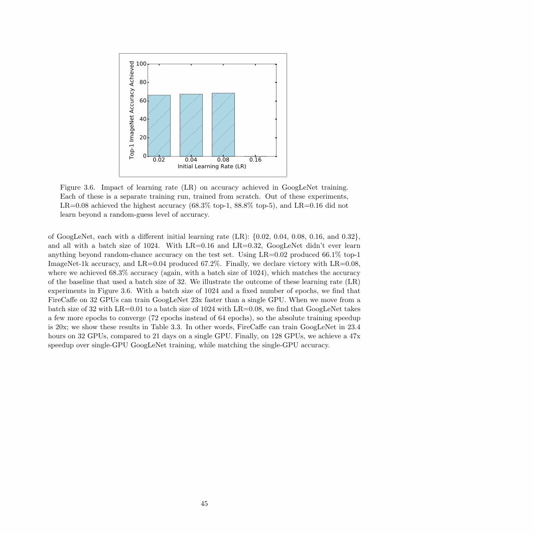
0.02 0.04 0.08 0.16Initial Learning Rate (LR)

0

20

40

60

80

100

Top-1

Im

ageN

et

Acc

ura

cy A

chie

ved

Figure 3.6. Impact of learning rate (LR) on accuracy achieved in GoogLeNet training.Each of these is a separate training run, trained from scratch. Out of these experiments,LR=0.08 achieved the highest accuracy (68.3% top-1, 88.8% top-5), and LR=0.16 did notlearn beyond a random-guess level of accuracy.

of GoogLeNet, each with a different initial learning rate (LR): {0.02, 0.04, 0.08, 0.16, and 0.32},and all with a batch size of 1024. With LR=0.16 and LR=0.32, GoogLeNet didn’t ever learnanything beyond random-chance accuracy on the test set. Using LR=0.02 produced 66.1% top-1ImageNet-1k accuracy, and LR=0.04 produced 67.2%. Finally, we declare victory with LR=0.08,where we achieved 68.3% accuracy (again, with a batch size of 1024), which matches the accuracyof the baseline that used a batch size of 32. We illustrate the outcome of these learning rate (LR)experiments in Figure 3.6. With a batch size of 1024 and a fixed number of epochs, we find thatFireCaffe on 32 GPUs can train GoogLeNet 23x faster than a single GPU. When we move from abatch size of 32 with LR=0.01 to a batch size of 1024 with LR=0.08, we find that GoogLeNet takesa few more epochs to converge (72 epochs instead of 64 epochs), so the absolute training speedupis 20x; we show these results in Table 3.3. In other words, FireCaffe can train GoogLeNet in 23.4hours on 32 GPUs, compared to 21 days on a single GPU. Finally, on 128 GPUs, we achieve a 47xspeedup over single-GPU GoogLeNet training, while matching the single-GPU accuracy.

45

Table 3.3. Accelerating the training of ultra-deep, computationally intensive models onImageNet-1k.

Hardware Net Epochs Batch

size

Initial

Learn-

ing

Rate

Train

time

Speedup Top-1

Accu-

racy

Top-5

Accu-

racy

Caffe 1 NVIDIA

K20

GoogLeNet

[79]

64 32 0.01 21

days

1x 68.3% 88.7%

FireCaffe

(ours)

32 NVIDIA

K20s (Titan

supercom-

puter)

GoogLeNet 72 1024 0.08 23.4

hours

20x 68.3% 88.7%

FireCaffe

(ours)

128 NVIDIA

K20s (Titan

supercom-

puter)

GoogLeNet 72 1024 0.08 10.5

hours

47x 68.3% 88.7%

3.8 Complementary approaches to accelerate DNN training

We have discussed related work throughout the chapter, but we now provide a brief survey ofadditional techniques to accelerate deep neural network training. Several of the following techniquescould be used in concert with FireCaffe to further accelerate DNN training.

3.8.1 Accelerating convolution on GPUs

In the DNN architectures discussed in this chapter, more than 90% of the floating-point op-erations in forward and backward propagation reside in convolution layers, so accelerating con-volution is key to getting the most out of each GPU. Recently, a number of techniques havebeen developed to accelerate convolution on GPUs. Unlike CPUs, NVIDIA GPUs have an in-verted memory hierarchy, where the register file is larger than the L1 cache. Volkov and Dem-mel [123] pioneered a communication-avoiding strategy to accelerate matrix multiplication onGPUs by staging as much data as possible in registers while maximizing data reuse. Iandolaet al. [50] extended the communication-avoiding techniques to accelerate 2D convolution; andcuDNN [25] and maxDNN [96] extended the techniques to accelerate 3D convolution. The Bodaframework [19, 26, 53] further extended the techniques to execute efficiently on GPU hardwareproduced by companies other than NVIDIA. FireCaffe can be coupled with current and futureGPU hardware and convolution libraries for further speedups.

46

3.8.2 Decreasing communication among servers

Reducing the quantity of data communicated per batch is a useful way to increase the speed andscalability of DNN training. There is an inherent tradeoff here: as gradients are more aggressivelyquantized, training speed goes up, but the model’s accuracy may go down compared to a non-quantized baseline. While FireCaffe uses 32-bit floating-point values for weight gradients, JeffreyDean stated in a recent keynote speech that Google often uses 16-bit floating-point values forcommunication between servers in DNN training [124]. Along the same lines, Wawrzynek et al. used16-bit weights and 8-bit activations in distributed neural network training [102]. Going one stepfurther, Seide et al. used 1-bit gradients for backpropagation, albeit with a drop in the accuracyof the trained model [125]. Finally, a related strategy to reduce communication between servers isto discard (and not communicate) gradients whose numerical values fall below a certain threshold.Amazon presented such a thresholding strategy in a recent paper on scaling up DNN training forspeech recognition [112]. However, Amazon’s evaluation uses a proprietary dataset, so it is notclear how this type of thresholding impacts the accuracy compared to a well-understood baseline.

So far in this section, we have discussed strategies for compressing or quantizing data to com-municate in distributed DNN training. There has also been a series of studies on applying di-mensionality reduction to DNNs once they have been trained. Jaderberg et al. [126] and Zhanget al. [127] both use PCA to compress the weights of DNN models by up to 5x, albeit with asubstantial reduction in the model’s classification accuracy. Han et al. [128] use a combination ofpruning, quantization, and Huffman encoding to compress the weights of pretrained models by 35xwith no reduction in accuracy. Thus far, these algorithms have only been able to accelerate DNNsat test time.

3.9 Conclusions

Long training times impose a severe limitation on progress in deep neural network research andproductization. Accelerating DNN training has several benefits. First, faster DNN training enablesmodels to be trained on ever-increasing dataset sizes in a tractable amount of time. AcceleratingDNN training also enables product teams to bring DNN-based products to market more rapidly.Finally, there are a number of compelling use-cases for real-time DNN training, such as robot self-learning. These and other compelling applications led us to focus on the problem of acceleratingDNN training, and our work has culminated in the FireCaffe distributed DNN training system.

Our approach to accelerating DNN training at scale has three key pillars. First, we selectnetwork hardware that achieves high bandwidth between GPU servers — Infiniband or Cray in-terconnects are ideal for this. Second, when selecting a communication algorithm, we find thatreduction trees are more efficient and scalable than the traditional parameter server approach.Third, we optionally increase the batch size to reduce the total quantity of communication duringDNN training, and we identify hyperparameters that allow us to reproduce the small-batch accu-racy while training with large batch sizes. These three pillars helped us to achieve a near-linearspeedup for a number of leading deep neural network architectures. In particular, we have achieved39x speedup on NiN training, and a 47x speedup on GoogLeNet training on a 128 GPU cluster.

47

Chapter 4

Defining and describing the design

space of DNN architectures

4.1 Introduction

Convolutional neural network (CNN) architectures comprise an enormous design space. ByCNN architecture, we mean:

• the type(s) of layers to use,

• the number of layers,

• the ordering/organization of layers, and

• the dimensions of each layer.

These are design choices that are specified by a human CNN architect. Each CNN architecturedelivers a specific set of tradeoffs in terms of accuracy, computational complexity, energy-efficiency,model size, and other metrics.

While it is true that there are only a handful of commonly-used CNN computational primitives(e.g. convolution, pooling, dropout, etc), there are many ways of arranging these primitives into adeep neural network architecture. The composition and total number of layers is selected by theCNN architect, and considering that some recent CNN architectures have 1000 layers or more (e.g.Highway Networks [129] and Residual Networks [15]), there is an exponentially large number ofpermutations in which different types of CNN layers can be composed. Further, within each layer,there are a number of dimensions to be selected by the CNN architect — e.g. in a convolutionlayer, the number of filters and spatial resolution of filters are user-selectable. Thus, the designspace of CNN architectures is enormous.

48

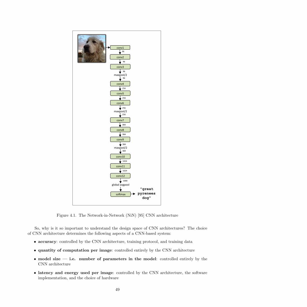
"great pyrenees

dog"

conv1&96&

conv2&96&

conv3&96&

conv4&256&

conv5&256&

conv6&

1000&

so/max&

maxpool/2&

global&avgpool&

96&

conv7&384&

conv8&384&

conv9&

maxpool/2&256&

256&

conv10&1024&

conv11&1024&

conv12&

maxpool/2&384&

384&

Figure 4.1. The Network-in-Network (NiN) [95] CNN architecture

So, why is it so important to understand the design space of CNN architectures? The choiceof CNN architecture determines the following aspects of a CNN-based system:

• accuracy: controlled by the CNN architecture, training protocol, and training data

• quantity of computation per image: controlled entirely by the CNN architecture

• model size — i.e. number of parameters in the model: controlled entirely by theCNN architecture

• latency and energy used per image: controlled by the CNN architecture, the softwareimplementation, and the choice of hardware

49

Thus, given specific and aggressive goals (e.g. in terms of accuracy, computation, speed, and/orenergy), achieving these goals requires a comprehensive understanding of the CNN architecturalspace.

This chapter is organized as follows. In Section 4.2, we describe the key building blocks (i.e.layers) of modern CNNs. In Section 4.3, we explain the geometrical properties of individual CNNlayers. Stacking multiple layers to form an end-to-end CNN leads to certain geometrical propertiesbeing passed from one layer to the next. In Section 4.4, we provide an intuitive mental model forunderstanding how changing the dimensions of one CNN layer can impact the overall quantity ofcomputation in a CNN. We explain the ways in which modifying dimensions of one CNN layerimpacts the dimensions of downstream layers in Sections 4.5 and 4.6. Clearly, CNNs comprise alarge design space, but how large is it? We provide some intuition on this in Section 4.7. Whilethis chapter focuses on CNN architectures, there are a number of additional design choices thatinfluence the time and accuracy level achieved during training, such as: (a) the choice of how toinitialize model parameters prior to training the model and (b) the solver approach used to trainthe model. We summarize some of the present literature on these design choices in Section 4.8. Weconclude in Section 4.9.

4.2 Key building blocks of CNN architectures

4.2.1 Convolution layers

4.2.1.1 The widespread use of convolution in computer vision

For more than forty years, convolution has been used widely in image processing and computervision. For example, the process of obtaining an RGB image from a CCD camera involves convo-lution using a filter called a Bayer mask [130]. Likewise, one of the most straightforward ways todetect edges — the Sobel Filter — consists entirely of convolving an image with a particular 3x3filter [131]. Canny edge detection also involves convolving an image with a filter — typically a 5x5filter where the numerical values in the filter are set based on a Gaussian distribution [132]. Withthese examples in mind, it should be no surprise that convolution is a key ingredient in applyingneural networks to computer vision problems. In convolutional neural networks, we apply manylayers of convolution, e.g. classification = conv layer(conv layer(...conv layer(image))).1 Whilethe previous examples (Bayer mask, Sobel filter, Canny edge detection) use filters in which thenumerical values were hand-selected by engineers, convolutional neural networks learn the filters’numerical values from their training data.

4.2.1.2 Introduction to the dimensionality of convolution layers in CNNs

Recall that our high-level objectives for this dissertation include decreasing the number of pa-rameters in CNNs and accelerating CNN training by decreasing the computational requirements.If we want to decrease the computational requirements of CNNs, we must first understand how

1Typically with nonlinearity functions placed between the convolution layers.

50

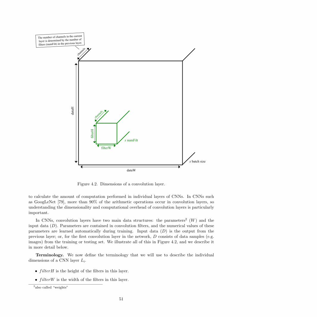
filterW

filte

rH

data

H

dataW

The number of channels in the current

layer is determined by the number of

filters (numFilt) in the previous layer.

x numFilt

TODO:%%•  different%color%for%

ac#va#ons(vs%filters(•  show%stride%somehow?%•  …%%%

x batch size

Figure 4.2. Dimensions of a convolution layer.

to calculate the amount of computation performed in individual layers of CNNs. In CNNs suchas GoogLeNet [79], more than 90% of the arithmetic operations occur in convolution layers, sounderstanding the dimensionality and computational overhead of convolution layers is particularlyimportant.

In CNNs, convolution layers have two main data structures: the parameters2 (W ) and theinput data (D). Parameters are contained in convolution filters, and the numerical values of theseparameters are learned automatically during training. Input data (D) is the output from theprevious layer; or, for the first convolution layer in the network, D consists of data samples (e.g.images) from the training or testing set. We illustrate all of this in Figure 4.2, and we describe itin more detail below.

Terminology. We now define the terminology that we will use to describe the individualdimensions of a CNN layer Li.

• filterH is the height of the filters in this layer.

• filterW is the width of the filters in this layer.

2also called “weights”

51

• numFilt is the number of filters in this layer. Each of these filters is of size filterH x filterWx ch.

• ch the number of channels the input data to this layer. Also, ch is the number of channels ineach filter. This is defined by numFilt in the previous layer.

• dataH is the height of the input data to this layer.

• dataW is the width of the input data to this layer.

• batch size is the number of data samples to which the CNN is applied concurrently. (SeeChapter 3, Section 3.3 for details.)

Some of these dimensions are inherited from the previous layer (Li−1) in the CNN: dataH, dataW ,and ch. Other dimensions are selected by the CNN architect: filterH, filterW , and numFilt.

Parameters (W ). In a convolution layer, W has 4 dimensions: filterH, filterW , ch, andnumFilt. The filters of W have a spatial resolution of filterHxfilterW , e.g. 1x1 or 3x3. Eachfilter has multiple channels ch — for example, if there are 3 input channels, then each filter hasch = 3. Finally, there are usually multiple convolution filters (numFilt), and each filter learns adifferent pattern to identify in the D. It can be difficult for humans to reason in 4 dimensions, sowe recommend taking extra care to avoid forgetting that every convolution layer has multiple filters(numFilt), and each of those filters has multiple channels (ch). The total quantity of parametersin a layer is filterH ∗ filterW ∗ ch ∗ numFilt, and it is common to represent each parameter as a4-byte floating-point number.

Input Data (D) for the first convolution layer. When training a CNN with batchedstochastic gradient descent (SGD), D has 4 dimensions: dataH, dataW , ch, and batch. The batchsize (batch) is user-selected, and batch is consistent over all convolution layers in the CNN. For thefirst layer in a CNN3 (L1), the input data (D0) is a batch of data samples (e.g. images) to trainon, and dataH, dataW , and ch are the height, width, and number of channels (e.g. 3 channels forRGB) of the training images.

Input Data (D) for later convolution layers. Now, let us consider a CNN layer Li wherei > 1, and the input data is the output from the previous layer, Li−1. Thus, for Li, the height andwidth of D — dataH, dataW — is determined by the output of the previous layer. For Li, thenumber of channels in the input data is determined by the number of filters (numFilt) in Li−1.Finally, as in L1, the batch size in Li is user-selected and is constant over all layers in the CNN.

4.2.2 Downsampling and Pooling

In convolutional neural networks, it is common to take an RGB image (e.g. 256x256x3) as inputand produce a vector (e.g. 1x1xNumberOfCategories) as output. Indeed, by default, CNNs suchas GoogLeNet [79], AlexNet [22], and SqueezeNet [18] take an RGB image as input and produce avector of classifications as output. But, how do we convert data with a spatial resolution such as256x256 into a data structure without spatial resolution (e.g. 1x1)? The answer is quite simple:we gradually downsample from 256x256 to 1x1. We do not downsample all at once; rather, in adeep network, we typically downsample once every few layers.

3In our notation, the “first” layer is directly after the input data, and the “last” layer is the one that outputs thefinal classifications.

52

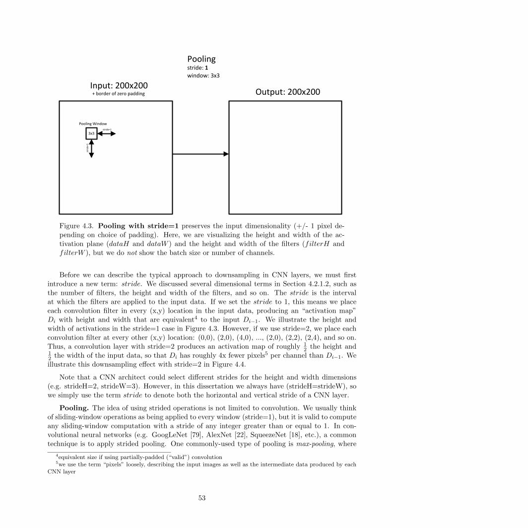
Inspired)by)slide)6)of)this:)h3ps://courses.cs.washington.edu/courses/cse590v/14au/cse590v_dec5_DeepVis.pdf)))Has)a)useful)animaFon)of)stride=1)conv:)h3p://www.wildml.com/2015/11/understandingIconvoluFonalIneuralInetworksI)forInlp/))

Input:)200x200)+)border)of)zero)padding) Output:)200x200)

Pooling)Window)stride=1)

strid

e=1)

3x3)

Pooling)stride:)1"window:)3x3)

Figure 4.3. Pooling with stride=1 preserves the input dimensionality (+/- 1 pixel de-pending on choice of padding). Here, we are visualizing the height and width of the ac-tivation plane (dataH and dataW ) and the height and width of the filters (filterH andfilterW ), but we do not show the batch size or number of channels.

Before we can describe the typical approach to downsampling in CNN layers, we must firstintroduce a new term: stride. We discussed several dimensional terms in Section 4.2.1.2, such asthe number of filters, the height and width of the filters, and so on. The stride is the intervalat which the filters are applied to the input data. If we set the stride to 1, this means we placeeach convolution filter in every (x,y) location in the input data, producing an “activation map”Di with height and width that are equivalent4 to the input Di−1. We illustrate the height andwidth of activations in the stride=1 case in Figure 4.3. However, if we use stride=2, we place eachconvolution filter at every other (x,y) location: (0,0), (2,0), (4,0), ..., (2,0), (2,2), (2,4), and so on.Thus, a convolution layer with stride=2 produces an activation map of roughly 1

2 the height and12 the width of the input data, so that Di has roughly 4x fewer pixels5 per channel than Di−1. Weillustrate this downsampling effect with stride=2 in Figure 4.4.

Note that a CNN architect could select different strides for the height and width dimensions(e.g. strideH=2, strideW=3). However, in this dissertation we always have (strideH=strideW), sowe simply use the term stride to denote both the horizontal and vertical stride of a CNN layer.

Pooling. The idea of using strided operations is not limited to convolution. We usually thinkof sliding-window operations as being applied to every window (stride=1), but it is valid to computeany sliding-window computation with a stride of any integer greater than or equal to 1. In con-volutional neural networks (e.g. GoogLeNet [79], AlexNet [22], SqueezeNet [18], etc.), a commontechnique is to apply strided pooling. One commonly-used type of pooling is max-pooling, where

4equivalent size if using partially-padded (“valid”) convolution5we use the term “pixels” loosely, describing the input images as well as the intermediate data produced by each

CNN layer

53

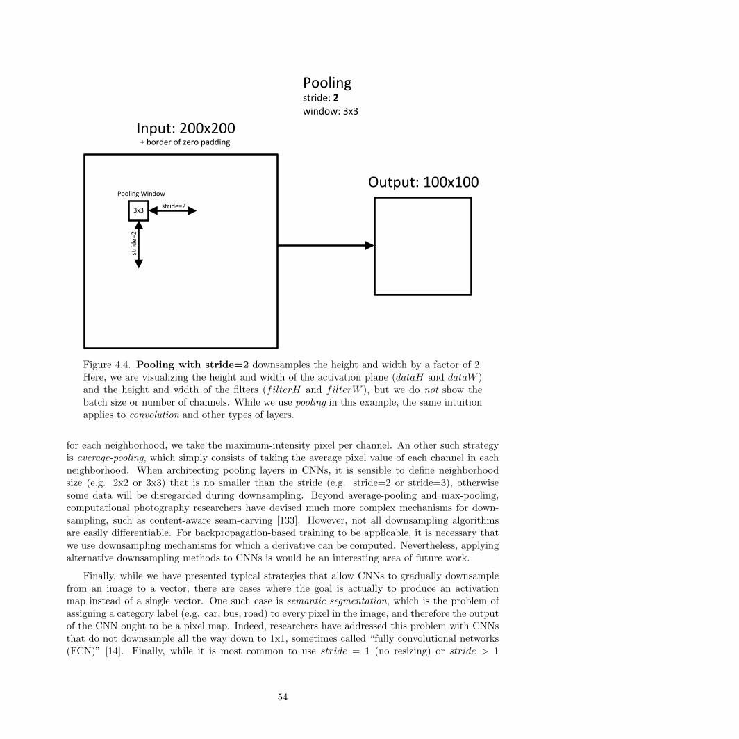
Inspired)by)slide)6)of)this:)h3ps://courses.cs.washington.edu/courses/cse590v/14au/cse590v_dec5_DeepVis.pdf)))Has)a)useful)animaFon)of)stride=1)conv:)h3p://www.wildml.com/2015/11/understandingIconvoluFonalIneuralInetworksI)forInlp/))

Input:)200x200)+)border)of)zero)padding)

Output:)100x100)Pooling)Window)

stride=2)

strid

e=2)

3x3)

Pooling)stride:)2"window:)3x3)

Figure 4.4. Pooling with stride=2 downsamples the height and width by a factor of 2.Here, we are visualizing the height and width of the activation plane (dataH and dataW )and the height and width of the filters (filterH and filterW ), but we do not show thebatch size or number of channels. While we use pooling in this example, the same intuitionapplies to convolution and other types of layers.

for each neighborhood, we take the maximum-intensity pixel per channel. An other such strategyis average-pooling, which simply consists of taking the average pixel value of each channel in eachneighborhood. When architecting pooling layers in CNNs, it is sensible to define neighborhoodsize (e.g. 2x2 or 3x3) that is no smaller than the stride (e.g. stride=2 or stride=3), otherwisesome data will be disregarded during downsampling. Beyond average-pooling and max-pooling,computational photography researchers have devised much more complex mechanisms for down-sampling, such as content-aware seam-carving [133]. However, not all downsampling algorithmsare easily differentiable. For backpropagation-based training to be applicable, it is necessary thatwe use downsampling mechanisms for which a derivative can be computed. Nevertheless, applyingalternative downsampling methods to CNNs is would be an interesting area of future work.

Finally, while we have presented typical strategies that allow CNNs to gradually downsamplefrom an image to a vector, there are cases where the goal is actually to produce an activationmap instead of a single vector. One such case is semantic segmentation, which is the problem ofassigning a category label (e.g. car, bus, road) to every pixel in the image, and therefore the outputof the CNN ought to be a pixel map. Indeed, researchers have addressed this problem with CNNsthat do not downsample all the way down to 1x1, sometimes called “fully convolutional networks(FCN)” [14]. Finally, while it is most common to use stride = 1 (no resizing) or stride > 1

54

(downsampling), work such as [14] also uses fractional strides (stride < 1) to upsample/enlarge thedataH and dataW .

4.2.3 Activation function layer

If a CNN were literally just a series of convolution layers and nothing else, the model wouldsimply be a linear system. Linear systems are a fairly constrained subset of what can be achievedwith deep networks. To express non-linear functions, it is common to introduce a nonlinearity intothe output of each convolution layer of a CNN. These nonlinearity functions are sometimes calledactivation functions. Note that, in diagrams of CNNs, the activation function is often omitted forbrevity. Also, in some CNN implementations and frameworks such as Caffe [106], the activationfunction is implemented as its own layer in the CNN.

In historical and recent literature, a number of activation functions have been proposed andapplied to CNNs. We do not attempt to provide an exhaustive survey of activation functions, butwe provide a few examples below:

• Hyperbolic tangent activation [134]: f(x) = tanh(x)

• Sigmoid activation [135]: f(x) = 11−exp(−x)

• Rectified linear unit (ReLU) activation [136]: f(x) = max(0, x)

• Variants of ReLU, including: ELU [137], PReLU [138], and Leaky ReLU [139].

For a more exhaustive discussion of activation functions, see the recent survey paper by Gu etal. [140].

The choice of activation function can have two main effects on how a CNN behaves:

1. Quantity of computation required to converge. Given a CNN, changing the per-layeractivation functions may change the number of epochs of training required to converge to aparticular level of accuracy.

2. Accuracy achieved during training. Given a CNN, changing the per-layer activationfunctions may change the accuracy that can be achieved during training. In pathologicalcases, certain choices of activation function may lead to the CNN not learning anything atall and remaining at a very low accuracy level.

The ramifications of the activation function are almost entirely constrained to the trainingphase, and it has little impact on the computational requirements during inference. This is becausethe quantity of computation required to calculate a typical activation function (e.g. ReLU: f(x) =max(0, x)) is extremely trivial compared to running a typical convolution layer over the same data.Therefore, the quantity of computation in most CNNs is dominated by layers such as convolution,and activation functions typically represent much less than 1% of the total quantity of computation.

55

4.2.4 Loss function layers

During training a loss function — sometimes called an objective function — is typically appliedat the end of the CNN6. The ideal choice of loss function (typically implemented as its own layerin the CNN) is highly dependent on the problem at hand. Without going into deep mathematicaldetails, we find that there are two main questions that a CNN architect must ask when beginningthe search for the “right” loss function:

1. Classification or regression? Do we want to train the CNN to solve a classification- orregression-style problem? In the classification formulation, it is typical to say “there are 100labels, and every data sample needs to be assigned to one of these labels.” Image classifica-tion (as in the running ImageNet example in Chapter 3) is one example where classificationobjective functions are sensible. On the other hand, in the regression formulation, it is typicalto say “for every every data sample, the sample needs to be analyzed, where the output is afloating-point number between -50 and 50.” Some loss functions, such as logistic regression,can be applied to either classification or regression [141]. Other loss functions — e.g. softmax— are specific to classification. Note that many of the loss functions used in CNNs were notdesigned specifically for CNN training — rather, they are loss functions that were developedin other areas of mathematical optimization and have been appropriated by CNN researchers.More examples of classification or regression loss functions can be found in [141] and [142].

2. One loss function or multiple loss functions? While it’s typical to optimize a CNN forone particular loss function, it’s possible to have multiple loss functions. A common exampleis to optimize a CNN to classify objects (using classification loss) and simultaneously optimizethe CNN to localize objects in (using regression loss) [13, 143]. Taken together, these twoloss functions train the CNN to perform object detection.

For an in-depth discussion of loss functions, we direct the interested reader to [141, 142].

4.2.5 Regularization function layers

In machine learning, the loss function is often formulated such that achieving zero loss (i.e.perfect convergence) on the training set can be done by simply memorizing the training set. Thisis problematic, because the real world (i.e. the test set and beyond) tends to be more diverse thanthe training set. The case where a machine-learned model memorizes the training set but deliverspoor accuracy on the test set is called overfitting.

Regularization refers to a family of techniques that can be used to combat overfitting. Roughlyspeaking, a method is a regularizer if it makes it more difficult to for a model to memorize thetraining set. In most cases, regularization is applied during training, but not during inference.

These are two of the most widely-used regularization methods in modern CNN/DNN research:

• Dropout [144]: if(rand=1), f(x)=0. else, f(x)=x.

• Batch Normalization [116]7: f(x1:batchsize) = x1:batchsize−mean(x1:batchsize)variance(x1:batchsize)

6In our nomenclature, the input data is the “beginning” and the loss function is the “end” of the CNN.7Using the straightforward Batch Normalization formulation that was presented in Chapter 8 of [145].

56

4.3 Understanding the dimensionality of CNN layers

4.3.1 How many parameters are in a convolution layer?

Consider a convolution layer Li that has 100 filters of spatial resolution filterH x filterW =3x3. How many parameters does this layer have? It might be tempting to answer 100*3*3=900,but you would be wrong!

In reality, we haven’t given you enough information to answer the question. You need to knowthe number of channels in the input data to Li. As we discussed in Section 4.2.1.2, for layer Li>1,the number of input channels (chi) is determined by the number of filters in the previous layer(numFilti−1). And, the first layer L1 is a special case: the number of input channels chi=1 isdetermined by the number of channels in the input data to the CNN. To keep our math simple, forthe first layer we use numFilti−1 as a shorthand for “the number of channels in the input data tothe CNN.” Now, let us turn our attention back to the present example. If the previous layer Li−1has 10 filters, then Li has 10 input channels, and Li has chi ∗ numFilti ∗ filterWi ∗ filterHi =10*100*3*3=9000 parameters. If you thought 900, then you were off by a factor of 10!

Here, we have considered the number of parameters in just one layer. Calculating the totalquantity of parameters in an entire CNN architecture is simply a matter of summing chi∗numFilti∗filterWi ∗ filterHi over layers i = 1 : n. We expressed this mathematically in terms of bytes inChapter 3, Equation 3.1, and we reproduce the equation below.

|W | =#layers∑L=1

numFiltL−1 ∗ numFiltL ∗ filterWL ∗ filterHL ∗ 4 (4.1)

Note that the the “∗ 4” assumes that we are representing the parameters in the filters as 4-bytefloating-point values. The “∗ 4” should be adjusted when representing the parameters with adifferent number of bytes (e.g. “∗ 2” for 16-bit floating-point values).

4.3.2 How big are the activation maps produced by a convolution layer?

Consider a convolution layer Li with 100 filters of size filterHi x filterWi = 3x3, stridei=2,and no zero-padding (padHi = padWi = 0). Note that the stride of 2 applies in the height andwidth dimensions. Also, the input data to Li is dataHi−1 x dataWi−1 x chi−1 = 50x50x10. Finally,assume that the batch size is 200. What is the dimensionality of the output data produced by Li?

We know that the number of output channels is 100, because it says above that Li has 100

filters (numFilti). We compute the height of the output activations (dataHi) as

dataHi = ceil(dataHi−1 + 2 ∗ padHi − filterHi

stridei) + 1 (4.2)

Plugging in the numbers for the present example, this works out to ceil(50+0−32 ) + 1 = 25. We

were given that dataHi = dataWi = 50, so the output width is also 25. Putting it all together, theoutput activation map from Li is batch x numFilti x dataHi x dataWi = 200x100x25x25.

57

4.3.3 How many arithmetic operations are performed in a convolution layer?

So far, we have discussed how to calculate the dimensionality and quantity of parameters andactivations in a convolution layer. Given the dimensionality of the parameters and the dimension-ality of the activations that a convolution layer produces as output, this is enough information tocalculate the quantity of computation in the layer.

As we have discussed in previous sections, a CNN architect is charged with defining certaindimensions for each convolution layer L. These dimensions include the height and width of filters(filterHL and filterWL), the number of filters in the previous layer (numFiltL−1), the numberof filters in the current layer (numFiltL), the height and width of output activations (dataHL anddataWidthL). Using these dimensions, we can compute the number of arithmetic operations inconvolution layer L as follows:

FLOPSL = numFiltL−1 ∗ numFiltL ∗ filterWL ∗ filterHL ∗ dataWL ∗ dataHL ∗ 2. (4.3)

Note that the factor of 2 is to account for the fact that the calculations use multiply-add calcula-tions, which count as two arithmetic operations.

Calculating the total quantity of computation in a CNN’s convolution layers is as simple assumming Equation 4.3 over all layers:

FLOPStotal =

#layers∑L=1

numFiltL−1 ∗ numFiltL ∗ filterWL ∗ filterHL ∗ dataWL ∗ dataHL ∗ 2. (4.4)

So far, we have concentrated on calculating the quantity of computation required for the infer-ence. While inference requires computing the forward pass only, training requires computing boththe forward and backward pass. The backward pass requires 2x more computation than the forwardpass, because the backward pass requires computing gradients with respect to the weights (∇W )and gradients with respect to the data (∇D). The computations of ∇W and ∇D each require thesame quantity of computation as the entire forward pass. Therefore, per image or data sample,training requires three times the quantity of computation that is required for inference [78]. In otherwords, to determine the quantity of computation per data sample during training, the procedureis simply to calculate Equation 4.4 and multiply the result by 3.

4.4 A mental model for how CNN dimensions impact the quantity

of computation and other metrics

Much research has been conducted on some aspects of CNNs such as (1) solvers [146, 147], (2)adding residual connections that skip over layers of CNNs [129, 15, 18], and (3) rethinking howto initialize parameters prior to training CNNs [113, 138]. All of these areas of research have animpact on the time required to train a CNN, and the end accuracy that is achieved. However, dothese topics affect the inference speed when it comes to deploy the CNN for a real application?For the most part, no. Solvers and parameter initialization are only relevant during training.

58

The residual connections that have appeared in recent literature [129, 15, 18] have a negligibleeffect on the inference speed, because they account for a tiny portion of the overall quantity ofcomputation. So, what factors do influence the speed or quantity of computation required duringinference time? Simply put, the CNN architecture and the dimensionality of the input dataare wholly responsible for determining the quantity of computation required during inference.8 Toour knowledge, there are few papers or documents that provide practical intuition on how CNNlayer dimensions impact the overall computational footprint. To remedy this, we have codified ourown mental model for understanding how changing the dimensions of a CNN impact the CNN’squantity of computation during inference.

Given a CNN, there are a number of ways to modify it in the interest of maximizing accuracy,minimizing the quantity of computation, or optimizing for other metrics. While there are manymodifications that we can make to a CNN, the modifications that have the most impact on thequantity of computation tend to deal with the number of channels or filters in layers or the heightand width of activations that are passed from one layer to the next. Some of the key ways ofmodifying a CNN include:

• changing the number of channels in the input data, e.g. adding a depth channel or concate-nating multiple video frames. (Section 4.5.2);

• changing the number of filters in a convolution layer (Section 4.5.3);

• changing the spatial resolution (height and/or width) of convolution filters in a layer (Section4.5.4);

• changing the number of categories classified by the CNN (Section 4.5.5);

• changing the quantity of downsampling performed in a convolution or pooling layer9 (Section4.6.1); or

• changing the spatial resolution of the input data (Section 4.6.2).

Initially, it may seem daunting to understand how each of these types of modifications affectthe quantity of computation required to perform inference in a CNN. Fortunately, all of thesemodifications can be distilled into a straightforward mental model. All of these CNN architecturalmodifications induce either a local change or a global change to the dimensions of the CNN, and wedefine these terms as follows.

1. Local change. We define a local change as the case where a modification to CNN layer Li

affects only the dimensionality of layer Li and possibly Li+1. Examples of a local changeinclude changing the number of channels in the input data (Section 4.5.2), changing the num-ber of filters in one convolution layer (Section 4.5.3), and changing the number of categoriesclassified by the CNN (Section 4.5.5).

2. Global change. In contrast to a local change, we define a global change as the case where amodification to CNN layer Li affects the dimensionality of layer Li and the subsequent layers(Li+1, ..., LN ). Examples of a global change include changing the resolution of the input im-ages (Section 4.6.2) and changing the strides of a convolution or pooling layer (Section 4.6.1).

8And, as we will see in Chapter 5, model compression can further impact the quantity of computation duringinference.

9e.g. by changing the strides or adding/removing a pooling layer

59

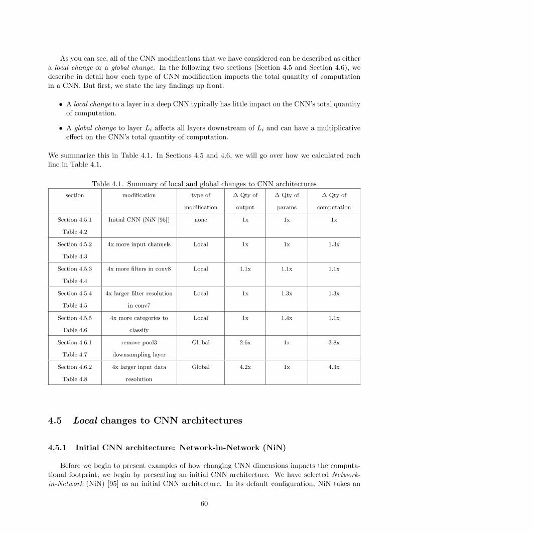
As you can see, all of the CNN modifications that we have considered can be described as eithera local change or a global change. In the following two sections (Section 4.5 and Section 4.6), wedescribe in detail how each type of CNN modification impacts the total quantity of computationin a CNN. But first, we state the key findings up front:

• A local change to a layer in a deep CNN typically has little impact on the CNN’s total quantityof computation.

• A global change to layer Li affects all layers downstream of Li and can have a multiplicativeeffect on the CNN’s total quantity of computation.

We summarize this in Table 4.1. In Sections 4.5 and 4.6, we will go over how we calculated eachline in Table 4.1.

Table 4.1. Summary of local and global changes to CNN architectures

section modification type of

modification

∆ Qty of

output

∆ Qty of

params

∆ Qty of

computation

Section 4.5.1

Table 4.2

Initial CNN (NiN [95]) none 1x 1x 1x

Section 4.5.2

Table 4.3

4x more input channels Local 1x 1x 1.3x

Section 4.5.3

Table 4.4

4x more filters in conv8 Local 1.1x 1.1x 1.1x

Section 4.5.4

Table 4.5

4x larger filter resolution

in conv7

Local 1x 1.3x 1.3x

Section 4.5.5

Table 4.6

4x more categories to

classify

Local 1x 1.4x 1.1x

Section 4.6.1

Table 4.7

remove pool3

downsampling layer

Global 2.6x 1x 3.8x

Section 4.6.2

Table 4.8

4x larger input data

resolution

Global 4.2x 1x 4.3x

4.5 Local changes to CNN architectures

4.5.1 Initial CNN architecture: Network-in-Network (NiN)

Before we begin to present examples of how changing CNN dimensions impacts the computa-tional footprint, we begin by presenting an initial CNN architecture. We have selected Network-in-Network (NiN) [95] as an initial CNN architecture. In its default configuration, NiN takes an

60

image as input, and it predicts the image’s category (e.g. “soup bowl” or “cowboy hat”) as output.In terms of accuracy, NiN is competitive with the highest-accuracy submissions in the ImageNet2012 and 2013 image classification challenges. The highest accuracy submission for ImageNet 2014— GoogLeNet [79] — draws inspiration from the NiN architecture.

We present an overview of the NiN architecture in Figure 4.1. We provide more detaileddimensions of the NiN architecture in Table 4.2. Observe that NiN has 12 convolution layers. Eachof these convolution layers has a multiple filters, where the filters are in the range from 1x1xChannelsto 11x11xChannels. In each layer, all filters are the same size. From beginning to end, NiN graduallydownsamples the height and width of the activations from 227x227 down to 1x1. The downsamplingis accomplished with max- and average-pooling, as well as (in the first convolutional layer) aconvolution stride of 2. In some CNNs such as AlexNet [22], the downsampling to 1x1xChannelsis done partway through the CNN, and the last few convolution layers (sometimes called “fully-connected layers” due to the special case of 1x1 dimensionality) operate without spatial resolution.However, every convolution layer in NiN has a spatial resolution greater than 1x1. After thefinal convolution layer, NiN does global average pooling, which means it takes the average of eachchannel’s (x,y) grid to downsample to 1x1xChannels. This design choice has a nice property:regardless of the input image height and width, NiN is able to output an output vector of size1x1xChannels.

For brevity, we have not shown all the details of NiN in Table 4.2. In this table, we have omittedthe following details:

• ReLU [136] is performed after each convolution layer.

• During training, Dropout [144] is performed after the 10th convolution layer.

• Batch Normalization [116] is not used at all in NiN.

• The initial layer (“data”) provides a batch of 3-channel (RGB) images.

• Each pooling layer has a stride of 2. When we say “a stride of 2,” we mean that both the x-and y-dimensions have a stride of 2. Within each convolution and pooling layer of NiN, thex- and y-dimensions have the same stride.

• As we discussed in Section 4.3, the number of filters (number of output channels) in convo-lution layer Li defines the number of input channels in convolution layer Li+1. In Table 4.2,to avoid redundancy we simply list the number of output channels in each layer.

• Pooling does not affect the number of channels (and pooling operates independently on eachchannel), so a pooling layer simply has the same number of output channels as the previousconvolution layer.

Observe in Table 4.2 that during inference with a batch size of 1024 images NiN produces5.90GB of output activations (for all layers combined), it has 30.4MB of filters (which is unaffectedby the batch size), and it requires 2.27TF of computation. In the following sections, we will showhow modifications to NiN impact the quantity of activations, the quantity of filters, and the quantityof computation required during inference.

61

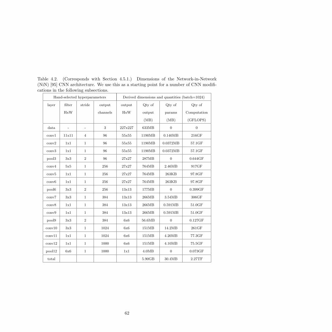
Table 4.2. (Corresponds with Section 4.5.1.) Dimensions of the Network-in-Network(NiN) [95] CNN architecture. We use this as a starting point for a number of CNN modifi-cations in the following subsections.

Hand-selected hyperparameters Derived dimensions and quantities (batch=1024)

layer filter

HxW

stride output

channels

output

HxW

Qty of

output

(MB)

Qty of

params

(MB)

Qty of

Computation

(GFLOPS)

data - - 3 227x227 633MB 0 0

conv1 11x11 4 96 55x55 1190MB 0.140MB 216GF

conv2 1x1 1 96 55x55 1190MB 0.0372MB 57.1GF

conv3 1x1 1 96 55x55 1190MB 0.0372MB 57.1GF

pool3 3x3 2 96 27x27 287MB 0 0.644GF

conv4 5x5 1 256 27x27 764MB 2.46MB 917GF

conv5 1x1 1 256 27x27 764MB 263KB 97.8GF

conv6 1x1 1 256 27x27 764MB 263KB 97.8GF

pool6 3x3 2 256 13x13 177MB 0 0.399GF

conv7 3x3 1 384 13x13 266MB 3.54MB 306GF

conv8 1x1 1 384 13x13 266MB 0.591MB 51.0GF

conv9 1x1 1 384 13x13 266MB 0.591MB 51.0GF

pool9 3x3 2 384 6x6 56.6MB 0 0.127GF

conv10 3x3 1 1024 6x6 151MB 14.2MB 261GF

conv11 1x1 1 1024 6x6 151MB 4.20MB 77.3GF

conv12 1x1 1 1000 6x6 151MB 4.10MB 75.5GF

pool12 6x6 1 1000 1x1 4.0MB 0 0.073GF

total 5.90GB 30.4MB 2.27TF

62

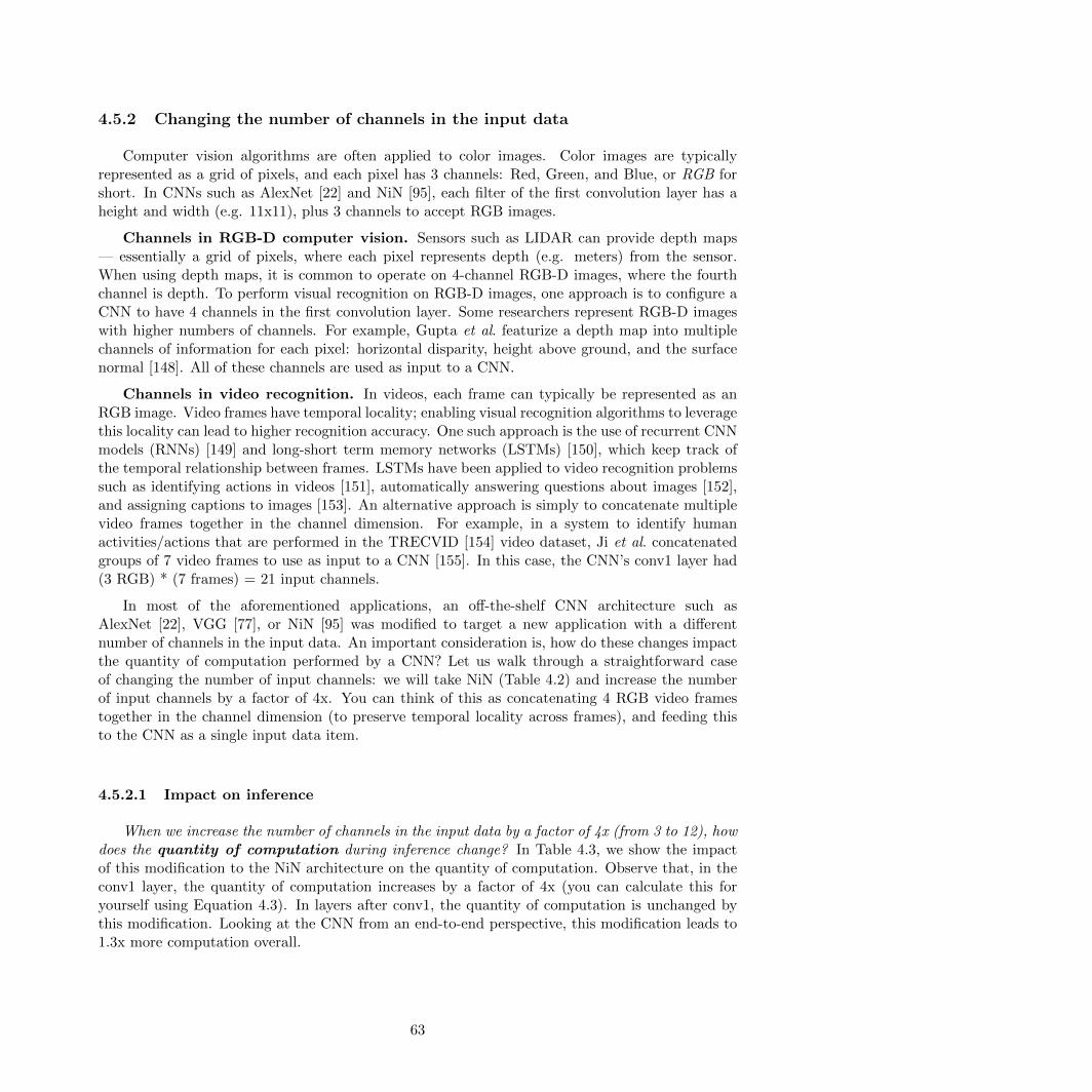
4.5.2 Changing the number of channels in the input data

Computer vision algorithms are often applied to color images. Color images are typicallyrepresented as a grid of pixels, and each pixel has 3 channels: Red, Green, and Blue, or RGB forshort. In CNNs such as AlexNet [22] and NiN [95], each filter of the first convolution layer has aheight and width (e.g. 11x11), plus 3 channels to accept RGB images.

Channels in RGB-D computer vision. Sensors such as LIDAR can provide depth maps— essentially a grid of pixels, where each pixel represents depth (e.g. meters) from the sensor.When using depth maps, it is common to operate on 4-channel RGB-D images, where the fourthchannel is depth. To perform visual recognition on RGB-D images, one approach is to configure aCNN to have 4 channels in the first convolution layer. Some researchers represent RGB-D imageswith higher numbers of channels. For example, Gupta et al. featurize a depth map into multiplechannels of information for each pixel: horizontal disparity, height above ground, and the surfacenormal [148]. All of these channels are used as input to a CNN.

Channels in video recognition. In videos, each frame can typically be represented as anRGB image. Video frames have temporal locality; enabling visual recognition algorithms to leveragethis locality can lead to higher recognition accuracy. One such approach is the use of recurrent CNNmodels (RNNs) [149] and long-short term memory networks (LSTMs) [150], which keep track ofthe temporal relationship between frames. LSTMs have been applied to video recognition problemssuch as identifying actions in videos [151], automatically answering questions about images [152],and assigning captions to images [153]. An alternative approach is simply to concatenate multiplevideo frames together in the channel dimension. For example, in a system to identify humanactivities/actions that are performed in the TRECVID [154] video dataset, Ji et al. concatenatedgroups of 7 video frames to use as input to a CNN [155]. In this case, the CNN’s conv1 layer had(3 RGB) * (7 frames) = 21 input channels.

In most of the aforementioned applications, an off-the-shelf CNN architecture such asAlexNet [22], VGG [77], or NiN [95] was modified to target a new application with a differentnumber of channels in the input data. An important consideration is, how do these changes impactthe quantity of computation performed by a CNN? Let us walk through a straightforward caseof changing the number of input channels: we will take NiN (Table 4.2) and increase the numberof input channels by a factor of 4x. You can think of this as concatenating 4 RGB video framestogether in the channel dimension (to preserve temporal locality across frames), and feeding thisto the CNN as a single input data item.

4.5.2.1 Impact on inference

When we increase the number of channels in the input data by a factor of 4x (from 3 to 12), howdoes the quantity of computation during inference change? In Table 4.3, we show the impactof this modification to the NiN architecture on the quantity of computation. Observe that, in theconv1 layer, the quantity of computation increases by a factor of 4x (you can calculate this foryourself using Equation 4.3). In layers after conv1, the quantity of computation is unchanged bythis modification. Looking at the CNN from an end-to-end perspective, this modification leads to1.3x more computation overall.

63

4.5.2.2 Impact on training

When we increase the number of channels in the input data by a factor of 4x (from 3 to 12),how does the time required to train a model (for a fixed number of epochs) change? In Table 4.3,we observe that this change requires 1.3x more computation10, but the quantity of parameters inthe CNN remains essentially unchanged. In the data-parallel training approach that we describedin Chapter 3, the quantity of communication sent and received by each server is determined bythe quantity of parameters in the CNN. Therefore, to answer the question stated above: whenwe increase the number of channels in the input data to the CNN, training on a fixed number ofprocessors is slightly slower. However, the ratio of computation

communication has increased, which means we canscale the modified CNN’s training problem to more processors and nearly regain the time-to-solutionthat is achievable with the original NiN model. Finally, note that the quantity of output (i.e. totalquantity of activations produced by all layers) does not affect the communication requirements indata-parallel distributed CNN training and therefore does not directly impact the scalability orspeed of training on multiple processors.

10Recall from Section 4.3.3 that CNN training requires 3x more computation per image than CNN inference.

64

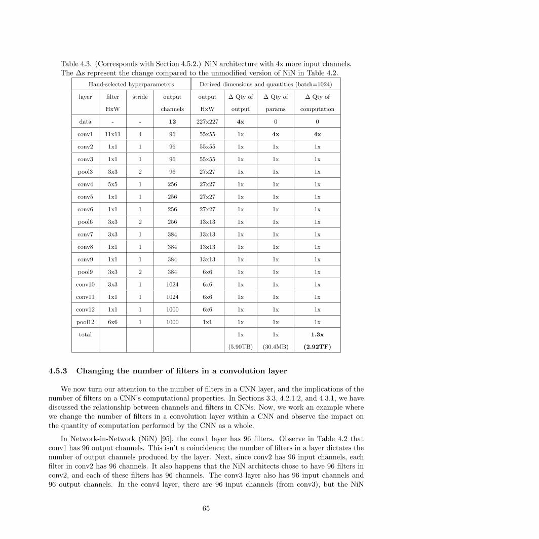
Table 4.3. (Corresponds with Section 4.5.2.) NiN architecture with 4x more input channels.The ∆s represent the change compared to the unmodified version of NiN in Table 4.2.


layer filter

HxW

stride output

channels

output

HxW

∆ Qty of

output

∆ Qty of

params

∆ Qty of

computation

data - - 12 227x227 4x 0 0

conv1 11x11 4 96 55x55 1x 4x 4x

conv2 1x1 1 96 55x55 1x 1x 1x

conv3 1x1 1 96 55x55 1x 1x 1x

pool3 3x3 2 96 27x27 1x 1x 1x

conv4 5x5 1 256 27x27 1x 1x 1x

conv5 1x1 1 256 27x27 1x 1x 1x

conv6 1x1 1 256 27x27 1x 1x 1x

pool6 3x3 2 256 13x13 1x 1x 1x

conv7 3x3 1 384 13x13 1x 1x 1x

conv8 1x1 1 384 13x13 1x 1x 1x

conv9 1x1 1 384 13x13 1x 1x 1x

pool9 3x3 2 384 6x6 1x 1x 1x

conv10 3x3 1 1024 6x6 1x 1x 1x

conv11 1x1 1 1024 6x6 1x 1x 1x

conv12 1x1 1 1000 6x6 1x 1x 1x

pool12 6x6 1 1000 1x1 1x 1x 1x

total 1x

(5.90TB)

1x

(30.4MB)

1.3x

(2.92TF)

4.5.3 Changing the number of filters in a convolution layer

We now turn our attention to the number of filters in a CNN layer, and the implications of thenumber of filters on a CNN’s computational properties. In Sections 3.3, 4.2.1.2, and 4.3.1, we havediscussed the relationship between channels and filters in CNNs. Now, we work an example wherewe change the number of filters in a convolution layer within a CNN and observe the impact onthe quantity of computation performed by the CNN as a whole.

In Network-in-Network (NiN) [95], the conv1 layer has 96 filters. Observe in Table 4.2 thatconv1 has 96 output channels. This isn’t a coincidence; the number of filters in a layer dictates thenumber of output channels produced by the layer. Next, since conv2 has 96 input channels, eachfilter in conv2 has 96 channels. It also happens that the NiN architects chose to have 96 filters inconv2, and each of these filters has 96 channels. The conv3 layer also has 96 input channels and96 output channels. In the conv4 layer, there are 96 input channels (from conv3), but the NiN

65

architects decided to have 256 filters in the conv4 layer. The NiN architects also decided to use aspatial resolution of 3x3 for the filters in conv4. Putting it all together, the conv4 layer has 256filters that are of size 3x3x96. From what we have learned so far, we can observe three propertiesof the number of filters in a CNN layer:

1. The number of filters in layer Li dictates the number of output channels in Li.

2. The number of input channels in Li+1 is equal to the number of output channels in Li.

3. Each filter has multiple channels. The number of filters in layer Li dictates the number ofchannels in each filter of layer Li+1.

The choice of the number of filters in CNN layers comprises a huge design space. With thisin mind, it is worthwhile to understand how the number of filters in a CNN layer impacts theoverall computational overhead of a CNN. To explore this, let us begin with the NiN architectureand increase the number of filters in the conv8 layer, and we will explore how this impacts thecomputational characteristics of the CNN.


When we increase the number of filters in conv8 by a factor of 4x (from 384 to 1536), howdoes the quantity of computation during inference change? Within conv8, the quantity ofcomputation increases by a factor of 4x; we can calculate this using Equation 4.3. Also, as wediscussed earlier in the section, the number of filters in layer Li defines the number of inputchannels to layer Li+1. Therefore, each filter in conv9 now has 4x more channels, leading to 4xmore computation in conv9.

However, in layers other than conv8 and conv9, the quantity of computation is unchanged. Aswe show in Table 4.4, the overall quantity of computation in the CNN increases by just 1.1x as aresult of increasing the number of filters in conv8 by 4x. Since increasing the number of filters ina layer impacts the quantity of computation in just 2 out of the 12 convolution layers, we describethis as a local change to a CNN architecture.


When we increase the number of filters in conv8 by a factor of 4x (from 384 to 1536), how doesthe time required to train a model (for a fixed number of epochs) change? This modification ledto a negligible 1.1x increase in both computation and model size (i.e. communication). Trainingthe model would be slightly more time-consuming. Since both the communication and computationincreased by the same amount, the problem’s distributed scalability remains unchanged.

66

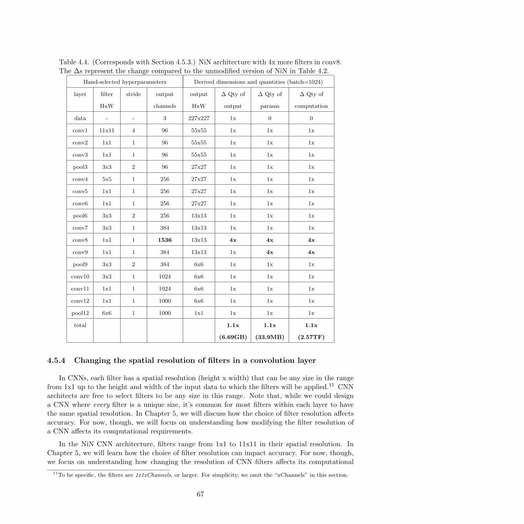
Table 4.4. (Corresponds with Section 4.5.3.) NiN architecture with 4x more filters in conv8.The ∆s represent the change compared to the unmodified version of NiN in Table 4.2.


layer filter

HxW

stride output

channels

output

HxW

∆ Qty of

output

∆ Qty of

params

∆ Qty of

computation

data - - 3 227x227 1x 0 0

conv1 11x11 4 96 55x55 1x 1x 1x

conv2 1x1 1 96 55x55 1x 1x 1x

conv3 1x1 1 96 55x55 1x 1x 1x

pool3 3x3 2 96 27x27 1x 1x 1x

conv4 5x5 1 256 27x27 1x 1x 1x

conv5 1x1 1 256 27x27 1x 1x 1x

conv6 1x1 1 256 27x27 1x 1x 1x

pool6 3x3 2 256 13x13 1x 1x 1x

conv7 3x3 1 384 13x13 1x 1x 1x

conv8 1x1 1 1536 13x13 4x 4x 4x

conv9 1x1 1 384 13x13 1x 4x 4x

pool9 3x3 2 384 6x6 1x 1x 1x

conv10 3x3 1 1024 6x6 1x 1x 1x

conv11 1x1 1 1024 6x6 1x 1x 1x

conv12 1x1 1 1000 6x6 1x 1x 1x

pool12 6x6 1 1000 1x1 1x 1x 1x

total 1.1x

(6.69GB)

1.1x

(33.9MB)

1.1x

(2.57TF)

4.5.4 Changing the spatial resolution of filters in a convolution layer

In CNNs, each filter has a spatial resolution (height x width) that can be any size in the rangefrom 1x1 up to the height and width of the input data to which the filters will be applied.11 CNNarchitects are free to select filters to be any size in this range. Note that, while we could designa CNN where every filter is a unique size, it’s common for most filters within each layer to havethe same spatial resolution. In Chapter 5, we will discuss how the choice of filter resolution affectsaccuracy. For now, though, we will focus on understanding how modifying the filter resolution ofa CNN affects its computational requirements.

In the NiN CNN architecture, filters range from 1x1 to 11x11 in their spatial resolution. InChapter 5, we will learn how the choice of filter resolution can impact accuracy. For now, though,we focus on understanding how changing the resolution of CNN filters affects its computational

11To be specific, the filters are 1x1xChannels, or larger. For simplicity, we omit the “xChannels” in this section.

67

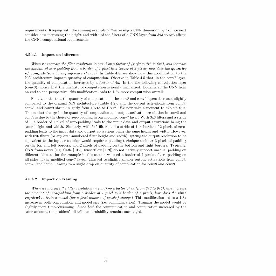
requirements. Keeping with the running example of “increasing a CNN dimension by 4x,” we nextconsider how increasing the height and width of the filters of a CNN layer from 3x3 to 6x6 affectsthe CNNs computational requirements.


When we increase the filter resolution in conv7 by a factor of 4x (from 3x3 to 6x6), and increasethe amount of zero-padding from a border of 1 pixel to a border of 2 pixels, how does the quantityof computation during inference change? In Table 4.5, we show how this modification to theNiN architecture impacts quantity of computation. Observe in Table 4.5 that, in the conv7 layer,the quantity of computation increases by a factor of 4x. In the the following convolution layer(conv8), notice that the quantity of computation is nearly unchanged. Looking at the CNN froman end-to-end perspective, this modification leads to 1.3x more computation overall.

Finally, notice that the quantity of computation in the conv8 and conv9 layers decreased slightlycompared to the original NiN architecture (Table 4.2), and the output activations from conv7,conv8, and conv9 shrunk slightly from 13x13 to 12x12. We now take a moment to explain this.The modest change in the quantity of computation and output activation resolution in conv8 andconv9 is due to the choice of zero-padding in our modified conv7 layer. With 3x3 filters and a strideof 1, a border of 1 pixel of zero-padding leads to the input data and output activations being thesame height and width. Similarly, with 5x5 filters and a stride of 1, a border of 2 pixels of zero-padding leads to the input data and output activations being the same height and width. However,with 6x6 filters (or any even-numbered filter height and width), getting the output resolution to beequivalent to the input resolution would require a padding technique such as: 3 pixels of paddingon the top and left borders, and 2 pixels of padding on the bottom and right borders. Typically,CNN frameworks (e.g. Caffe [106], TensorFlow [119]) do not natively support unequal padding ondifferent sides, so for the example in this section we used a border of 2 pixels of zero-padding onall sides in the modified conv7 layer. This led to slightly smaller output activations from conv7,conv8, and conv9, leading to a slight drop on quantity of computation for conv8 and conv9.


When we increase the filter resolution in conv7 by a factor of 4x (from 3x3 to 6x6), and increasethe amount of zero-padding from a border of 1 pixel to a border of 2 pixels, how does the timerequired to train a model (for a fixed number of epochs) change? This modification led to a 1.3xincrease in both computation and model size (i.e. communication). Training the model would beslightly more time-consuming. Since both the communication and computation increased by thesame amount, the problem’s distributed scalability remains unchanged.

68

Table 4.5. (Corresponds with Section 4.5.4.) NiN architecture with 4x larger filter resolutionin layer conv7 (3x3 → 6x6). The ∆s represent the change compared to the unmodifiedversion of NiN in Table 4.2.


layer filter

HxW

stride output

channels

output

HxW

∆ Qty of

output

∆ Qty of

params

∆ Qty of

computation

data - - 3 227x227 1x 0 0

conv1 11x11 4 96 55x55 1x 1x 1x

conv2 1x1 1 96 55x55 1x 1x 1x

conv3 1x1 1 96 55x55 1x 1x 1x

pool3 3x3 2 96 27x27 1x 1x 1x

conv4 5x5 1 256 27x27 1x 1x 1x

conv5 1x1 1 256 27x27 1x 1x 1x

conv6 1x1 1 256 27x27 1x 1x 1x

pool6 3x3 2 256 13x13 1x 1x 1x

conv7 6x6 1 384 12x12 0.8x 4x 3.4x

conv8 1x1 1 384 12x12 0.8x 1x 0.9x

conv9 1x1 1 384 12x12 0.8x 1x 0.9x

pool9 3x3 2 384 6x6 1x 1x 1x

conv10 3x3 1 1024 6x6 1x 1x 1x

conv11 1x1 1 1024 6x6 1x 1x 1x

conv12 1x1 1 1000 6x6 1x 1x 1x

pool12 6x6 1 1000 1x1 1x 1x 1x

total 1x

(5.82GB)

1.3x

(41.0MB)

1.3x

(2.99TF)

4.5.5 Changing the number of categories classified by a CNN

Applications of CNNs include single-class (i.e. binary) and multi-class classification. The out-put layer of a CNN has a number filters that is equal to the number of categories to be classified(i.e. the number of distinct categories in the training set). In the context of this section, wedefine “classification” inclusively to span (1) full-image classification (e.g. [18]), (2) localized recog-nition/detection (e.g. [156]), (3) semantic segmentation (e.g. [14]), and other applications. In all ofthese cases, there is a multi-class classification aspect to the problem: localized detection classifiesregions/windows of the images in terms of a list of object categories, and semantic segmentationclassifies pixels in terms of a list of visual categories. In all of these applications, the number offilters in the final layer is set equal to the number of classes in the training set.

Let us consider the NiN CNN architecture as a starting point. When trained on ImageNet,

69

the authors of NiN allocated 1000 filters in conv12 (the final layer), because ImageNet-1k has 1000categories of training and test data. Next, we consider the case where we would like to apply NiNto to a visual category recognition task with more categories — say, 4000 categories of images.


When we increase the number of categories in the dataset by a factor of 4x (from 1000 to4000), how does the quantity of computation during inference change? In Table 4.6, we showthe impact of this modification to NiN architecture on the quantity of computation. In the finalconvolution layer (conv12), there is one filter for each category in the dataset. So, the numberof filters in conv12 has increased from 1000 to 4000, leading to 4x more computation in conv12.However, the dimensionality and quantity of computation in all other layers remains unchanged.Looking at the CNN from an end-to-end perspective, this modification leads to just 1.1x morecomputation overall.


When we increase the number of categories in the dataset by a factor of 4x (from 1000 to 4000),how does the time required to train a model (for a fixed number of epochs) change? In Table 4.6,we observe that this change leads to a 1.4x larger model size (i.e. 1.4x more communication) and1.1x more computation. Therefore, the ratio of computation

communication has decreased, which tells us thatthis CNN is less scalable than the original NiN model. In other words, not only does this modelrequire more computation than the original NiN model, but the runtime will be dominated bycommunication at a smaller number of processors than in the case of the original NiN model. Forboth of these reasons, when using distributed data-parallel training, this model is slower to trainthan the original NiN model.

70

Table 4.6. (Corresponds with Section 4.5.5.) NiN architecture with 4x more categoriesto classify. The ∆s represent the change compared to the unmodified version of NiN inTable 4.2.


layer filter

HxW

stride output

channels

output

HxW

∆ Qty of

output

∆ Qty of

params

∆ Qty of

computation

data - - 3 227x227 1x 0 0

conv1 11x11 4 96 55x55 1x 1x 1x

conv2 1x1 1 96 55x55 1x 1x 1x

conv3 1x1 1 96 55x55 1x 1x 1x

pool3 3x3 2 96 27x27 1x 1x 1x

conv4 5x5 1 256 27x27 1x 1x 1x

conv5 1x1 1 256 27x27 1x 1x 1x

conv6 1x1 1 256 27x27 1x 1x 1x

pool6 3x3 2 256 13x13 1x 1x 1x

conv7 3x3 1 384 13x13 1x 1x 1x

conv8 1x1 1 384 13x13 1x 1x 1x

conv9 1x1 1 384 13x13 1x 1x 1x

pool9 3x3 2 384 6x6 1x 1x 1x

conv10 3x3 1 1024 6x6 1x 1x 1x

conv11 1x1 1 1024 6x6 1x 1x 1x

conv12 1x1 1 4000 6x6 4x 4x 4x

pool12 6x6 1 4000 1x1 4x 1x 4x

total 1x

(5.90GB)

1.4x

(42.6MB)

1.1x

(2.49TF)

4.5.6 Recap of local changes to CNN architectures

In the previous sections (4.5.2—4.5.5), we have considered a number local changes to CNNarchitectures. Under our terminology, a “local” change is one where modifying layer Li only affectsthe dimensions of layer Li and, in some cases, layer Li+1. The dimensions of other layers (Li+2, ...,Ln) are unaffected by a local change to layer Li. There is a common pattern among all of the localchanges that we have considered: the changes all involve modifying the dimensions of one layer’sfilters or channels. There is a reason for this: the number of filters in layer Li defines the numberof input channels in layer Li+1, but the number of filters in Li has no bearing on the number ofinput channels to layers Li+2, ..., Ln.

In contrast to the local changes that we have discussed so far, in the next section we will discuss

71

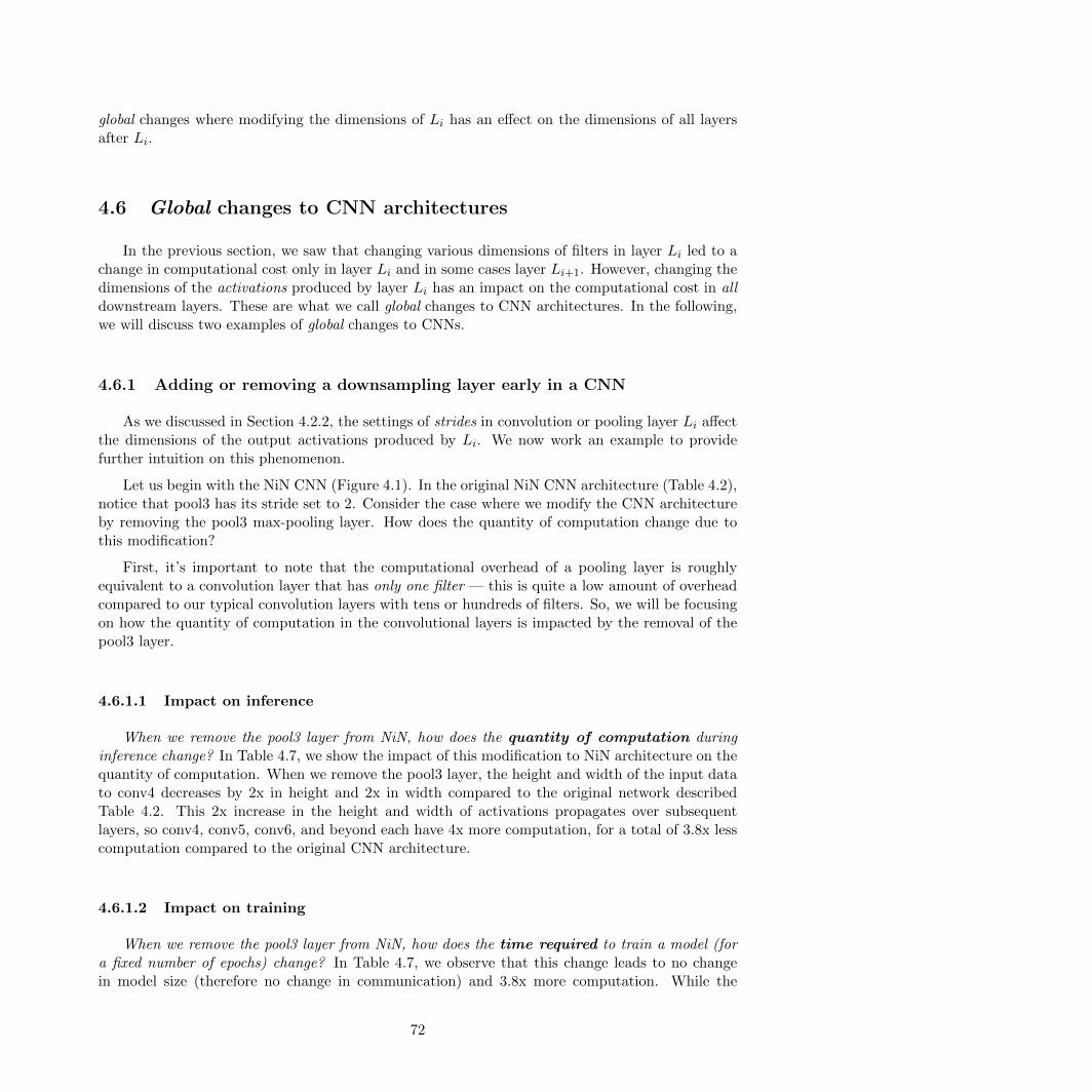
global changes where modifying the dimensions of Li has an effect on the dimensions of all layersafter Li.

4.6 Global changes to CNN architectures

In the previous section, we saw that changing various dimensions of filters in layer Li led to achange in computational cost only in layer Li and in some cases layer Li+1. However, changing thedimensions of the activations produced by layer Li has an impact on the computational cost in alldownstream layers. These are what we call global changes to CNN architectures. In the following,we will discuss two examples of global changes to CNNs.

4.6.1 Adding or removing a downsampling layer early in a CNN

As we discussed in Section 4.2.2, the settings of strides in convolution or pooling layer Li affectthe dimensions of the output activations produced by Li. We now work an example to providefurther intuition on this phenomenon.

Let us begin with the NiN CNN (Figure 4.1). In the original NiN CNN architecture (Table 4.2),notice that pool3 has its stride set to 2. Consider the case where we modify the CNN architectureby removing the pool3 max-pooling layer. How does the quantity of computation change due tothis modification?

First, it’s important to note that the computational overhead of a pooling layer is roughlyequivalent to a convolution layer that has only one filter — this is quite a low amount of overheadcompared to our typical convolution layers with tens or hundreds of filters. So, we will be focusingon how the quantity of computation in the convolutional layers is impacted by the removal of thepool3 layer.


When we remove the pool3 layer from NiN, how does the quantity of computation duringinference change? In Table 4.7, we show the impact of this modification to NiN architecture on thequantity of computation. When we remove the pool3 layer, the height and width of the input datato conv4 decreases by 2x in height and 2x in width compared to the original network describedTable 4.2. This 2x increase in the height and width of activations propagates over subsequentlayers, so conv4, conv5, conv6, and beyond each have 4x more computation, for a total of 3.8x lesscomputation compared to the original CNN architecture.


When we remove the pool3 layer from NiN, how does the time required to train a model (fora fixed number of epochs) change? In Table 4.7, we observe that this change leads to no changein model size (therefore no change in communication) and 3.8x more computation. While the

72

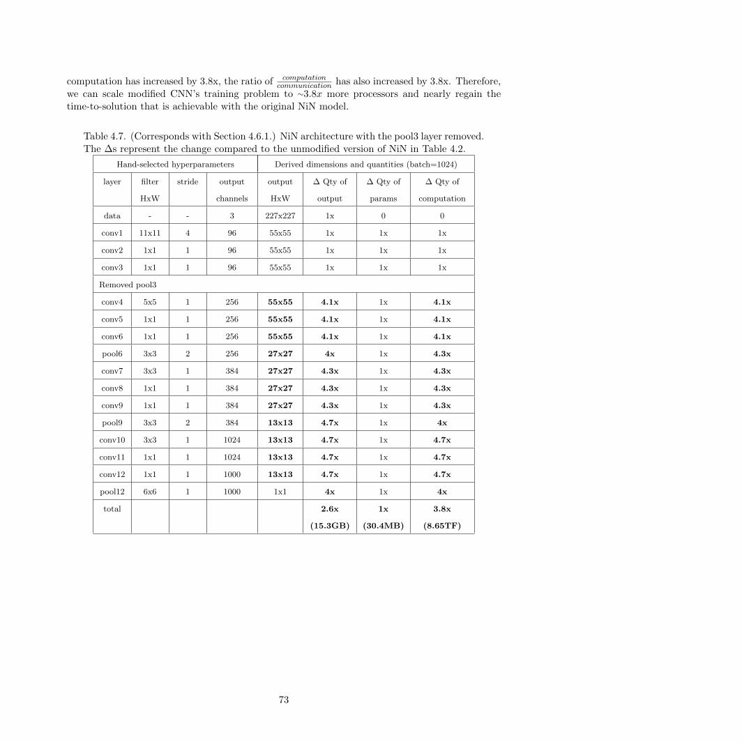
computation has increased by 3.8x, the ratio of computationcommunication has also increased by 3.8x. Therefore,

we can scale modified CNN’s training problem to ∼3.8x more processors and nearly regain thetime-to-solution that is achievable with the original NiN model.

Table 4.7. (Corresponds with Section 4.6.1.) NiN architecture with the pool3 layer removed.The ∆s represent the change compared to the unmodified version of NiN in Table 4.2.


layer filter

HxW

stride output

channels

output

HxW

∆ Qty of

output

∆ Qty of

params

∆ Qty of

computation

data - - 3 227x227 1x 0 0

conv1 11x11 4 96 55x55 1x 1x 1x

conv2 1x1 1 96 55x55 1x 1x 1x

conv3 1x1 1 96 55x55 1x 1x 1x

Removed pool3

conv4 5x5 1 256 55x55 4.1x 1x 4.1x

conv5 1x1 1 256 55x55 4.1x 1x 4.1x

conv6 1x1 1 256 55x55 4.1x 1x 4.1x

pool6 3x3 2 256 27x27 4x 1x 4.3x

conv7 3x3 1 384 27x27 4.3x 1x 4.3x

conv8 1x1 1 384 27x27 4.3x 1x 4.3x

conv9 1x1 1 384 27x27 4.3x 1x 4.3x

pool9 3x3 2 384 13x13 4.7x 1x 4x

conv10 3x3 1 1024 13x13 4.7x 1x 4.7x

conv11 1x1 1 1024 13x13 4.7x 1x 4.7x

conv12 1x1 1 1000 13x13 4.7x 1x 4.7x

pool12 6x6 1 1000 1x1 4x 1x 4x

total 2.6x

(15.3GB)

1x

(30.4MB)

3.8x

(8.65TF)

73

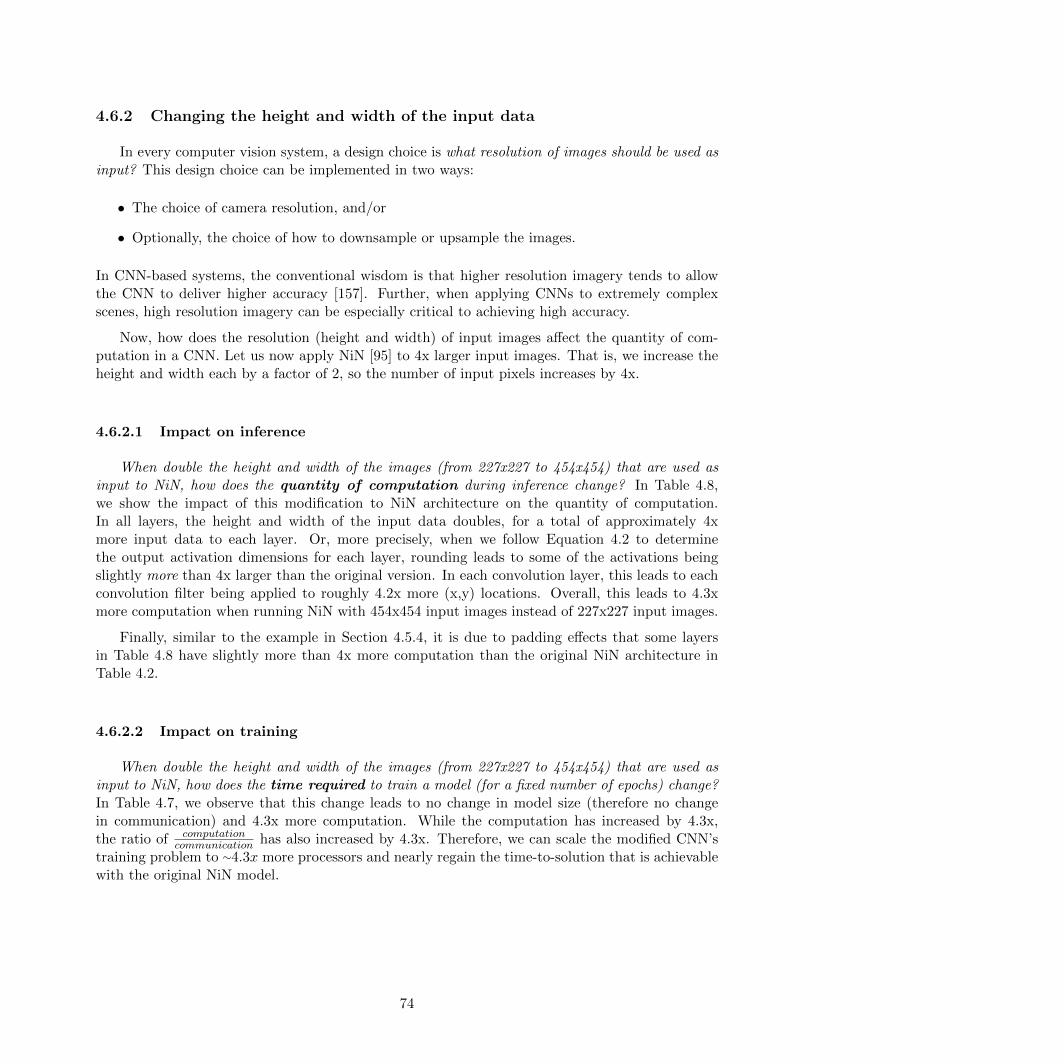
4.6.2 Changing the height and width of the input data

In every computer vision system, a design choice is what resolution of images should be used asinput? This design choice can be implemented in two ways:

• The choice of camera resolution, and/or

• Optionally, the choice of how to downsample or upsample the images.

In CNN-based systems, the conventional wisdom is that higher resolution imagery tends to allowthe CNN to deliver higher accuracy [157]. Further, when applying CNNs to extremely complexscenes, high resolution imagery can be especially critical to achieving high accuracy.

Now, how does the resolution (height and width) of input images affect the quantity of com-putation in a CNN. Let us now apply NiN [95] to 4x larger input images. That is, we increase theheight and width each by a factor of 2, so the number of input pixels increases by 4x.


When double the height and width of the images (from 227x227 to 454x454) that are used asinput to NiN, how does the quantity of computation during inference change? In Table 4.8,we show the impact of this modification to NiN architecture on the quantity of computation.In all layers, the height and width of the input data doubles, for a total of approximately 4xmore input data to each layer. Or, more precisely, when we follow Equation 4.2 to determinethe output activation dimensions for each layer, rounding leads to some of the activations beingslightly more than 4x larger than the original version. In each convolution layer, this leads to eachconvolution filter being applied to roughly 4.2x more (x,y) locations. Overall, this leads to 4.3xmore computation when running NiN with 454x454 input images instead of 227x227 input images.

Finally, similar to the example in Section 4.5.4, it is due to padding effects that some layersin Table 4.8 have slightly more than 4x more computation than the original NiN architecture inTable 4.2.


When double the height and width of the images (from 227x227 to 454x454) that are used asinput to NiN, how does the time required to train a model (for a fixed number of epochs) change?In Table 4.7, we observe that this change leads to no change in model size (therefore no changein communication) and 4.3x more computation. While the computation has increased by 4.3x,the ratio of computation

communication has also increased by 4.3x. Therefore, we can scale the modified CNN’straining problem to ∼4.3x more processors and nearly regain the time-to-solution that is achievablewith the original NiN model.

74

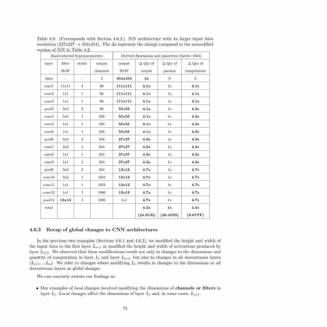
Table 4.8. (Corresponds with Section 4.6.2.) NiN architecture with 4x larger input dataresolution (227x227→ 454x454). The ∆s represent the change compared to the unmodifiedversion of NiN in Table 4.2.


layer filter

HxW

stride output

channels

output

HxW

∆ Qty of

output

∆ Qty of

params

∆ Qty of

computation

data - - 3 454x454 4x 0 0

conv1 11x11 4 96 111x111 4.1x 1x 4.1x

conv2 1x1 1 96 111x111 4.1x 1x 4.1x

conv3 1x1 1 96 111x111 4.1x 1x 4.1x

pool3 3x3 2 96 55x55 4.1x 1x 4.2x

conv4 5x5 1 256 55x55 4.1x 1x 4.2x

conv5 1x1 1 256 55x55 4.1x 1x 4.2x

conv6 1x1 1 256 55x55 4.1x 1x 4.2x

pool6 3x3 2 256 27x27 4.3x 1x 4.3x

conv7 3x3 1 384 27x27 4.3x 1x 4.3x

conv8 1x1 1 384 27x27 4.3x 1x 4.3x

conv9 1x1 1 384 27x27 4.3x 1x 4.3x

pool9 3x3 2 384 13x13 4.7x 1x 4.7x

conv10 3x3 1 1024 13x13 4.7x 1x 4.7x

conv11 1x1 1 1024 13x13 4.7x 1x 4.7x

conv12 1x1 1 1000 13x13 4.7x 1x 4.7x

pool12 13x13 1 1000 1x1 4.7x 1x 4.7x

total 4.2x

(24.5GB)

1x

(30.4MB)

4.3x

(9.67TF)

4.6.3 Recap of global changes to CNN architectures

In the previous two examples (Sections 4.6.1 and 4.6.2), we modified the height and width ofthe input data to the first layer Li=1 or modified the height and width of activations produced bylayer Li≥1. We observed that these modifications result not only in changes to the dimensions andquantity of computation in layer Li and layer Li+1, but also to changes in all downstream layers(Li+1, ...Ln). We refer to changes where modifying Li results in changes to the dimensions to alldownstream layers as global changes.

We can concisely restate our findings as:

• Our examples of local changes involved modifying the dimensions of channels or filters inlayer Li. Local changes affect the dimensions of layer Li and, in some cases, Li+1.

75

• Our examples of global changes involve modifying the dimensions of input data or activa-tions in layer Li. Global changes affect the dimensions of layers Li, ..., Ln.

4.7 Intuition on the size of the design space of CNNs

In Sections 4.5 and 4.6, we described seven different CNN architectures. How many more CNNarchitectures are there? We now work out a concrete example on the number of unique CNNarchitectures that exist in a particular sub-space of the CNN design space.

In the ImageNet 2012 and 2013 image-classification competitions, the winning approaches con-sisted of CNNs that had fewer than 10 layers. In ImageNet 2014 competition, the winners were theVGG-19 [77] 19-layer CNN model and the GoogLeNet [79] CNN model, which has over 20 layers.In their paper on VGG-19, Simonyan and Zisserman not only presented the VGG-19 architecture,but they also explored five variants of the VGG-19 architecture (for a total of six different archi-tectures). For the rest of this section, we use the CNN architectural space defined by Simonyanand Zisserman as the basis for a discussion on how large just a narrow corner of the overall CNNarchitectural space is.

The six CNN architectures presented by Simonyan and Zisserman have up to 19 layers, whichwe will enumerate as L1, ..., Ln [77]. In all of these models, layers Ln−2, Ln−1, andLn share thesame dimensions. The remaining convolution layers L1, ..., Ln−3 each have one of the following fivedimensional configurations:

1. 64 filters of size 3x3xnumFilti−1




5. 0 filters (i.e. “NULL layer”). We use this in our notation for VGG models that have fewerthan 19 layers.

So, how many unique CNNs can we create that have up to 16 convolution layers, each with one ofthe aforementioned dimensions?12 Mathematically, we have 16 layers (some which may be NULL),and each layer can be one of five different dimensions. This works out to 516 = 30 billion uniqueCNN architectures!

In this section we have shown that, even when given a narrow range of options for the type anddimensions for CNN layers, there are billions of unique combinations of these layers. However, thetruth is that this section has covered only a narrow corner of the CNN design space. As evidencethat the design space is much larger: to our knowledge, there are no known limits or upper-boundson several dimensions of CNNs, such as (a) the size of the input data, (b) the number of layers,and (c) the number of new types of layers that have yet to be invented. Considering all of thesefactors, we believe that, for most practical purposes, the design space of CNNs can be considered

12Or, to be more precise: we are viewing the VGG design space as “up to 16 layers, plus three layers Ln−2, Ln−1, Ln

that each have a fixed size.”

76

to be an infinitely large design space. In Chapter 5, we will present a strategy for choosing specificregions of the design space that are worthwhile to explore.

4.8 The design space of techniques for training CNNs

Given a particular problem (e.g. in the domain of text, audio, or vision) and the abilityto obtain appropriate labeled data to train models to solve the problem, a CNN architect mustcarefully consider and explore a number of design choices (DC’s) including the following:

• DC1. The design of the CNN architecture. (Covered in Sections 4.2—4.7.)

• DC2. The approach for initializing the CNN architecture’s model parameters prior to train-ing. (Covered in Section 4.8.1.)

• DC3. The optimization methodology or solver approach used to train the model. (Coveredin Section 4.8.2.)

We now present a few observations on the implications of these design choices, as well as how thesedesign choices have been covered in the literature so far.

CNN architecture (DC1). The dimensions and design principles of CNN architectures arediscussed in relatively little detail in the literature. Out of the thousands of computer vision andCNN papers that have appeared in the last few years, relatively few papers propose a substantiallynew CNN architecture, and it is even more rare to find papers that propose and evaluate manynew CNN architectures. Meanwhile, the choice of CNN architecture directly effects the quantity ofcomputation and the speed that can be achieved during both training and inference. The specificways in which the CNN architecture impacts the computational footprint is not widely discussedin the literature.

Model parameter initialization (DC2) and Solver approach (DC3). Model parameterinitialization and solver approaches are widely discussed in the literature. Optimization is a fieldwith a long history and a wide following, and many optimization experts have recently refocusedtheir careers on optimization methods for neural networks. The choice of how to initialize modelparameters and the choice of solver approach impacts the number of epochs (i.e. passes throughthe training set) required to achieve a given level of accuracy.13 Thus, DC2 and DC3 impact thequantity of computation and the time required to train CNN models. However, DC2 and DC3 donot impact the quantity of computation or achievable speed during inference. We summarize theeffects of DC1, DC2, and DC3 in Table 4.9.

Given that the CNN architecture (DC1) has limited coverage in the literature, and that DC1has the broadest impact on the CNN’s computational requirements, we have focused our discussionsin this chapter on DC1. However, for completeness we now summarize the current literature onmodel parameter initialization (DC2) and solver approaches (DC3), and we direct the interestedreader to resources for further reading.

13Further, DC2 and DC3 can influence the maximum accuracy that can be achieved when training a specific CNNarchitecture.

77

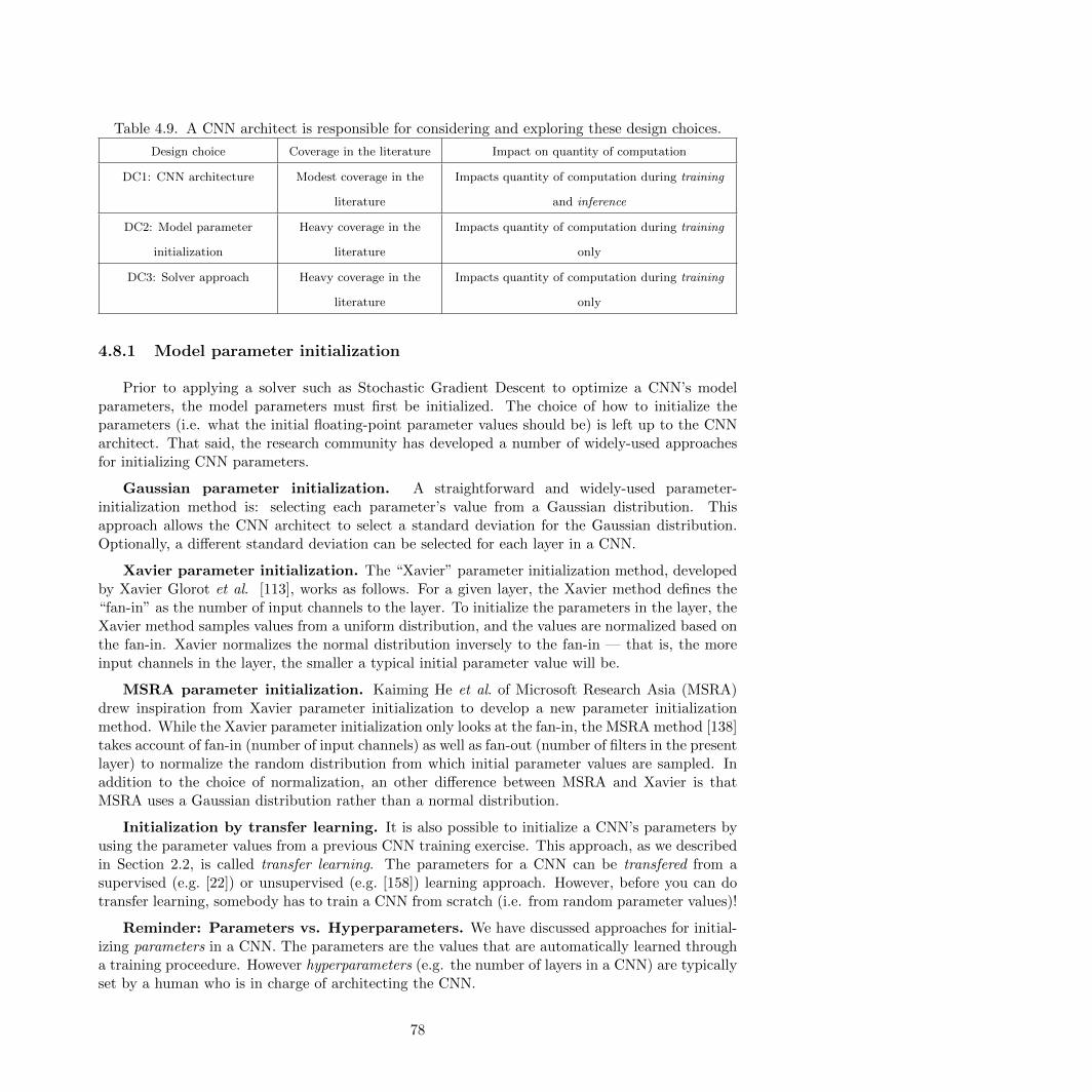
Table 4.9. A CNN architect is responsible for considering and exploring these design choices.

Design choice Coverage in the literature Impact on quantity of computation

DC1: CNN architecture Modest coverage in the

literature

Impacts quantity of computation during training

and inference

DC2: Model parameter

initialization

Heavy coverage in the

literature


only

DC3: Solver approach Heavy coverage in the

literature


only

4.8.1 Model parameter initialization

Prior to applying a solver such as Stochastic Gradient Descent to optimize a CNN’s modelparameters, the model parameters must first be initialized. The choice of how to initialize theparameters (i.e. what the initial floating-point parameter values should be) is left up to the CNNarchitect. That said, the research community has developed a number of widely-used approachesfor initializing CNN parameters.

Gaussian parameter initialization. A straightforward and widely-used parameter-initialization method is: selecting each parameter’s value from a Gaussian distribution. Thisapproach allows the CNN architect to select a standard deviation for the Gaussian distribution.Optionally, a different standard deviation can be selected for each layer in a CNN.

Xavier parameter initialization. The “Xavier” parameter initialization method, developedby Xavier Glorot et al. [113], works as follows. For a given layer, the Xavier method defines the“fan-in” as the number of input channels to the layer. To initialize the parameters in the layer, theXavier method samples values from a uniform distribution, and the values are normalized based onthe fan-in. Xavier normalizes the normal distribution inversely to the fan-in — that is, the moreinput channels in the layer, the smaller a typical initial parameter value will be.

MSRA parameter initialization. Kaiming He et al. of Microsoft Research Asia (MSRA)drew inspiration from Xavier parameter initialization to develop a new parameter initializationmethod. While the Xavier parameter initialization only looks at the fan-in, the MSRA method [138]takes account of fan-in (number of input channels) as well as fan-out (number of filters in the presentlayer) to normalize the random distribution from which initial parameter values are sampled. Inaddition to the choice of normalization, an other difference between MSRA and Xavier is thatMSRA uses a Gaussian distribution rather than a normal distribution.

Initialization by transfer learning. It is also possible to initialize a CNN’s parameters byusing the parameter values from a previous CNN training exercise. This approach, as we describedin Section 2.2, is called transfer learning. The parameters for a CNN can be transfered from asupervised (e.g. [22]) or unsupervised (e.g. [158]) learning approach. However, before you can dotransfer learning, somebody has to train a CNN from scratch (i.e. from random parameter values)!

Reminder: Parameters vs. Hyperparameters. We have discussed approaches for initial-izing parameters in a CNN. The parameters are the values that are automatically learned througha training proceedure. However hyperparameters (e.g. the number of layers in a CNN) are typicallyset by a human who is in charge of architecting the CNN.

78

4.8.2 Solver approaches

Once we have selected a CNN architecture and initialized its parameters, the next step isto train the CNN’s parameters so it can perform tasks such as identifying objects in images.Developing optimization approaches, or solvers, to train CNN parameters is an extremely activearea of research. We now present some of the current approaches to training CNNs.

In the present literature, Stochastic Gradient Descent (SGD) is the standard optimizationmethodology for training CNNs. SGD, as typically applied to CNNs, operates by taking a subset(a.k.a. batch) of the training data, attempting to classify it, and computing gradients that sum-marize the mistakes that were made when attempting to classify the data. Then backprogation isapplied to train each layer to avoid this mistake next time it sees a similar data sample.

With the goal of converging to higher accuracy, or converging to a given accuracy level withless computation, a number of SGD variants have been developed. We summarize some of theseSGD-based methods as follows.

• SGD with momentum aims to accelerate the learning process when faced with noisygradients [146].

• SGD with Nesterov momentum makes some further tweaks to the gradient update func-tion with the goal of requiring less computation to converge [147].

• Adagrad is an SGD-like optimization method that automatically selects a unique learningrate for each parameter in the neural network [159].

• RMSProp is an evolution of Adagrad that uses a moving average with exponential weight-ing [160].

For further reading, Chapter 8 of the Deep Learning textbook by Goodfellow et al. [145] explainsthe mathematical details of several popular forms of SGD.

4.9 Conclusions

CNN architects are responsible for several design decisions, including the choice of CNN archi-tecture, the choice of how to initialize the model parameters, and the choice of the solver approachto use for training the model. While parameter initialization and solver approaches have beenwidely covered in the literature, we have yet to find a useful guide on designing CNN architectures.To remedy this, we have focused this chapter on providing intuition about the dimensions of CNNlayers and how these dimensions impact the characteristics of an end-to-end CNN during trainingand inference. We summarize this intuition in a few key lessons:

• The number of channels in layer Li is dictated by the number of filters in the previous layerLi−1. For the first layer, L1, the number of channels is dictated by the input data (e.g. 3channels in RGB images). (Section 4.2)

• The quantity of computation, quantity of parameters, and quantity of activations in a layercan be calculated easily with closed-form mathematics. (Section 4.3)

79

• Modifications to the number of channels, number of filters, or spatial resolution of filters yieldlocal changes to a CNN’s dimensions. A local change to layer Li only impacts the dimensionof layer Li and in some cases Li+1. (Section 4.5)

• Modifications to the spatial resolution of input data or activations yield global changes to aCNN’s dimensions. A global change to layer Li impacts all following layers (Li+1, ..., Ln).(Section 4.6)

• CNNs comprise an enormous design space. Considering just a narrow corner of the CNNdesign space, we discovered that approximately 30 billion CNNs can be constructed. (Section4.7)

• There are a number of standard mechanisms for initializing the model parameters of a CNNand training a CNN. (Section 4.8)

80

Chapter 5

Exploring the design space of DNN

architectures

5.1 Introduction and motivation

Much of the recent research on deep convolutional neural networks (CNNs) has focused onincreasing accuracy on computer vision datasets. For a given accuracy level, there typically existmultiple CNN architectures that achieve that accuracy level. Given equivalent accuracy, a CNNarchitecture with fewer parameters has several advantages:

• More efficient distributed training. Communication among servers is the limiting factorto the scalability of distributed CNN training. For distributed data-parallel training, com-munication overhead is directly proportional to the number of parameters in the model [17].In short, small models train faster due to requiring less communication.

• Less overhead when exporting new models to clients. For autonomous driving, com-panies such as Tesla periodically copy new models from their servers to customers’ cars.This practice is often referred to as an over-the-air update. Consumer Reports has foundthat the safety of Tesla’s Autopilot semi-autonomous driving functionality has incrementallyimproved with recent over-the-air updates [161]. However, over-the-air updates of today’stypical CNN/DNN models can require large data transfers. With AlexNet, this would re-quire 240MB of communication from the server to the car. Smaller models require lesscommunication, making frequent updates more feasible.

• Feasible FPGA and embedded deployment. FPGAs often have less than 10MB1 of on-chip memory and no off-chip memory or storage. For inference, a sufficiently small model couldbe stored directly on the FPGA instead of being bottlenecked by memory bandwidth [94],while video frames stream through the FPGA in real time. Further, when deploying CNNs on

1For example, the Xilinx Vertex-7 FPGA has a maximum of 8.5 MBytes (i.e. 68 Mbits) of on-chip memory anddoes not provide off-chip memory.

81

Application-Specific Integrated Circuits (ASICs), a sufficiently small model could be storeddirectly on-chip, and smaller models may enable the ASIC to fit on a smaller die.

As you can see, there are several advantages of smaller CNN architectures. With this in mind,we focus directly on the problem of identifying a CNN architecture with fewer parameters butequivalent accuracy compared to a well-known model. We have identified such an architecture,which we call SqueezeNet. In addition, we present our attempt at a more disciplined approach tosearching the design space for novel CNN architectures.

The rest of the chapter is organized as follows. In Section 5.2 we review the related work.Then, in Sections 5.3 and 5.4 we describe and evaluate the SqueezeNet architecture. After that,we turn our attention to understanding how CNN architectural design choices impact model sizeand accuracy. We gain this understanding by exploring the design space of SqueezeNet-like archi-tectures. In Section 5.5, we do design space exploration on the CNN microarchitecture, which wedefine as the organization and dimensionality of individual layers and modules. In Section 5.6, wedo design space exploration on the CNN macroarchitecture, which we define as high-level organi-zation of layers in a CNN. Finally, we conclude in Section 5.7. In short, Sections 5.3 and 5.4 areuseful for CNN researchers as well as practitioners who simply want to apply SqueezeNet to a newapplication. The remaining sections are aimed at advanced researchers who intend to design theirown CNN architectures.

5.2 Related work

5.2.1 Model Compression

The overarching goal of our work is to identify a model that has very few parameters whilepreserving accuracy. To address this problem, a sensible approach is to take an existing CNNmodel and compress it in a lossy fashion. In fact, a research community has emerged around thetopic of model compression, and several approaches have been reported. A fairly straightforwardapproach by Denton et al. is to apply singular value decomposition (SVD) to a pretrained CNNmodel [162]. Han et al. developed Network Pruning, which begins with a pretrained model, thenreplaces parameters that are below a certain threshold with zeros to form a sparse matrix, and finallyperforms a few iterations of training on the sparse CNN [163]. Recently, Han et al. extended theirwork by combining Network Pruning with quantization (to 8 bits or less) and Huffman encodingto create an approach called Deep Compression [164], and further designed a hardware acceleratorcalled EIE [165] that operates directly on the compressed model, achieving substantial speedupsand energy savings.

5.2.2 CNN Microarchitecture

Convolutions have been used in artificial neural networks for at least 25 years; LeCun etal. helped to popularize CNNs for digit recognition applications in the late 1980s [166]. In neuralnetworks, convolution filters are typically 3D, with height, width, and channels as the key dimen-sions. When applied to images, CNN filters typically have 3 channels in their first layer (i.e. RGB),

82

and in each subsequent layer Li the filters have the same number of channels as Li−1 has filters. Theearly work by LeCun et al. [166] uses 5x5xChannels2 filters, and the recent VGG [77] architecturesextensively use 3x3 filters. Models such as Network-in-Network [95] and the GoogLeNet family ofarchitectures [79, 116, 167, 168] use 1x1 filters in some layers.

With the trend of designing very deep CNNs, it becomes cumbersome to manually select filterdimensions for each layer. To address this, various higher level building blocks, or modules, com-prised of multiple convolution layers with a specific fixed organization have been proposed. Forexample, the GoogLeNet papers propose Inception modules, which are comprised of a number ofdifferent dimensionalities of filters, usually including 1x1 and 3x3, plus sometimes 5x5 [79] andsometimes 1x3 and 3x1 [167]. Many such modules are then combined, perhaps with additionalad-hoc layers, to form a complete network. We use the term CNN microarchitecture to refer to theparticular organization and dimensions of the individual modules.

5.2.3 CNN Macroarchitecture

While the CNN microarchitecture refers to individual layers and modules, we define the CNNmacroarchitecture as the system-level organization of multiple modules into an end-to-end CNNarchitecture.

Perhaps the mostly widely studied CNN macroarchitecture topic in the recent literature is theimpact of depth (i.e. number of layers) in networks. Simoyan and Zisserman proposed the VGG [77]family of CNNs with 12 to 19 layers and reported that deeper networks produce higher accuracyon the ImageNet-1k dataset [21]. K. He et al. proposed deeper CNNs with up to 30 layers thatdeliver even higher ImageNet accuracy [138].

The choice of connections across multiple layers or modules is an emerging area of CNN macroar-chitectural research. Residual Networks (ResNet) [15] and Highway Networks [129] each proposethe use of connections that skip over multiple layers, for example additively connecting the ac-tivations from layer 3 to the activations from layer 6. We refer to these connections as bypassconnections. The authors of ResNet provide an A/B comparison of a 34-layer CNN with and with-out bypass connections; adding bypass connections delivers a 2 percentage-point improvement onTop-5 ImageNet accuracy.

5.2.4 Neural Network Design Space Exploration

Neural networks (including deep and convolutional NNs) have a large design space, with nu-merous options for microarchitectures, macroarchitectures, solvers, and other hyperparameters. Itseems natural that the community would want to gain intuition about how these factors impact aNN’s accuracy (i.e. the shape of the design space). Much of the work on design space exploration(DSE) of NNs has focused on developing automated approaches for finding NN architectures thatdeliver higher accuracy. These automated DSE approaches include Bayesian optimization [169],simulated annealing [170], randomized search [171], and genetic algorithms [172]. To their credit,each of these papers provides a case in which the proposed DSE approach produces a NN architec-ture that achieves higher accuracy compared to a representative baseline. However, these papers

2From now on, we will simply abbreviate HxWxChannels to HxW.

83

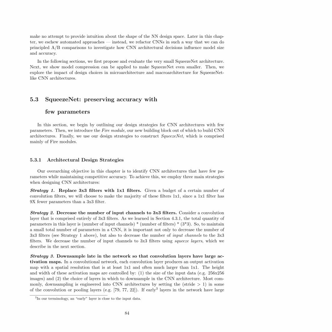
make no attempt to provide intuition about the shape of the NN design space. Later in this chap-ter, we eschew automated approaches — instead, we refactor CNNs in such a way that we can doprincipled A/B comparisons to investigate how CNN architectural decisions influence model sizeand accuracy.

In the following sections, we first propose and evaluate the very small SqueezeNet architecture.Next, we show model compression can be applied to make SqueezeNet even smaller. Then, weexplore the impact of design choices in microarchitecture and macroarchitecture for SqueezeNet-like CNN architectures.

5.3 SqueezeNet: preserving accuracy with

few parameters

In this section, we begin by outlining our design strategies for CNN architectures with fewparameters. Then, we introduce the Fire module, our new building block out of which to build CNNarchitectures. Finally, we use our design strategies to construct SqueezeNet, which is comprisedmainly of Fire modules.

5.3.1 Architectural Design Strategies

Our overarching objective in this chapter is to identify CNN architectures that have few pa-rameters while maintaining competitive accuracy. To achieve this, we employ three main strategieswhen designing CNN architectures:

Strategy 1. Replace 3x3 filters with 1x1 filters. Given a budget of a certain number ofconvolution filters, we will choose to make the majority of these filters 1x1, since a 1x1 filter has9X fewer parameters than a 3x3 filter.

Strategy 2. Decrease the number of input channels to 3x3 filters. Consider a convolutionlayer that is comprised entirely of 3x3 filters. As we learned in Section 4.3.1, the total quantity ofparameters in this layer is (number of input channels) * (number of filters) * (3*3). So, to maintaina small total number of parameters in a CNN, it is important not only to decrease the number of3x3 filters (see Strategy 1 above), but also to decrease the number of input channels to the 3x3filters. We decrease the number of input channels to 3x3 filters using squeeze layers, which wedescribe in the next section.

Strategy 3. Downsample late in the network so that convolution layers have large ac-tivation maps. In a convolutional network, each convolution layer produces an output activationmap with a spatial resolution that is at least 1x1 and often much larger than 1x1. The heightand width of these activation maps are controlled by: (1) the size of the input data (e.g. 256x256images) and (2) the choice of layers in which to downsample in the CNN architecture. Most com-monly, downsampling is engineered into CNN architectures by setting the (stride > 1) in someof the convolution or pooling layers (e.g. [79, 77, 22]). If early3 layers in the network have large

3In our terminology, an “early” layer is close to the input data.

84

h"p://www.presenta.on0process.com/lego0blocks0in0powerpoint.html88

squeeze8

expand8

1x18convolu.on8filters8

1x18and83x38convolu.on8filters8

ReLU8

ReLU8

Figure 5.1. Microarchitectural view: Organization of convolution filters in the Fire mod-ule. In this example, s1x1 = 3, e1x1 = 4, and e3x3 = 4. We illustrate the convolution filtersbut not the activations.

strides, then most layers will have small activation maps. Conversely, if most layers in the networkhave a stride of 1, and the strides greater than 1 are concentrated toward the end4 of the network,then many layers in the network will have large activation maps. Our intuition is that large ac-tivation maps (due to delayed downsampling) can lead to higher classification accuracy, with allelse held equal. Indeed, K. He and H. Sun applied delayed downsampling to four different CNNarchitectures, and in each case delayed downsampling led to higher classification accuracy [78].

Strategies 1 and 2 are about judiciously decreasing the quantity of parameters in a CNN whileattempting to preserve accuracy. Strategy 3 is about maximizing accuracy on a limited budget ofparameters. Next, we describe the Fire module, which is our building block for CNN architecturesthat enables us to successfully employ Strategies 1, 2, and 3.

5.3.2 The Fire Module

We define the Fire module as follows. A Fire module is comprised of a squeeze convolution layer(which has only 1x1 filters), feeding into an expand layer that has a mix of 1x1 and 3x3 convolutionfilters; we illustrate this in Figure 5.1. The liberal use of 1x1 filters in Fire modules is an applicationof Strategy 1 from Section 5.3.1. We expose three tunable dimensions (hyperparameters) in a Firemodule: s1x1, e1x1, and e3x3. In a Fire module, s1x1 is the number of filters in the squeeze layer(all 1x1), e1x1 is the number of 1x1 filters in the expand layer, and e3x3 is the number of 3x3 filtersin the expand layer. When we use Fire modules we set s1x1 to be less than (e1x1 + e3x3), so thesqueeze layer helps to limit the number of input channels to the 3x3 filters, as per Strategy 2 fromSection 5.3.1.

4In our terminology, the “end” of the network is the classifier.

85

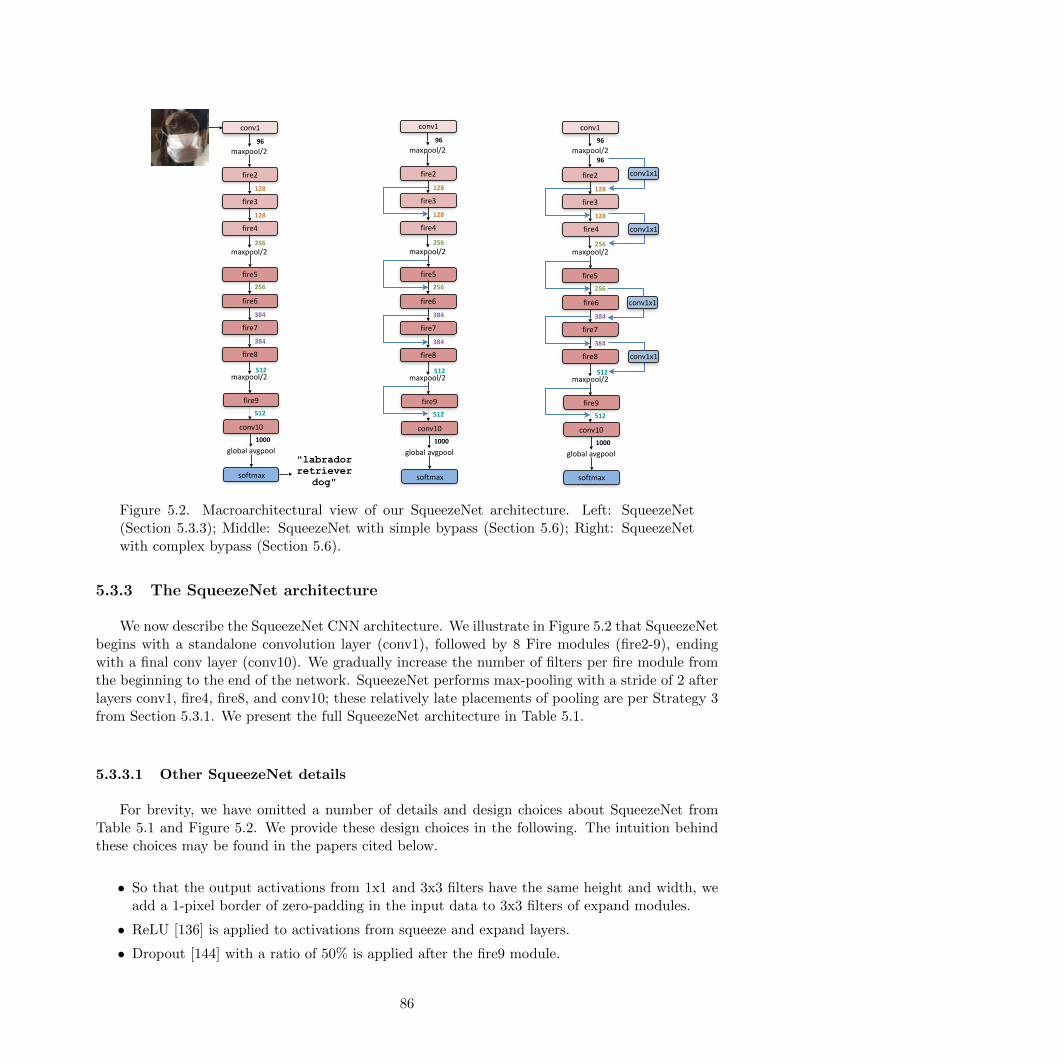
"labrador retriever

dog"

conv1

96

fire2

128

fire3

128

fire4

256

fire5256

fire6

384

fire7

384

fire8

512

fire9512

conv101000

softmax

maxpool/2

maxpool/2

maxpool/2

globalavgpool

conv1

96

fire2

128

fire3

128

fire4

256

fire5256

fire6

384

fire7

384

fire8

512

fire9512

conv101000

softmax

maxpool/2

maxpool/2

maxpool/2

globalavgpool

conv196

fire2

128

fire3

128

fire4

256

fire5256

fire6

384

fire7

384

fire8

512

fire9512

conv101000

softmax

maxpool/2

maxpool/2

maxpool/2

globalavgpool

conv1x1

conv1x1

conv1x1

conv1x1

96

Figure 5.2. Macroarchitectural view of our SqueezeNet architecture. Left: SqueezeNet(Section 5.3.3); Middle: SqueezeNet with simple bypass (Section 5.6); Right: SqueezeNetwith complex bypass (Section 5.6).

5.3.3 The SqueezeNet architecture

We now describe the SqueezeNet CNN architecture. We illustrate in Figure 5.2 that SqueezeNetbegins with a standalone convolution layer (conv1), followed by 8 Fire modules (fire2-9), endingwith a final conv layer (conv10). We gradually increase the number of filters per fire module fromthe beginning to the end of the network. SqueezeNet performs max-pooling with a stride of 2 afterlayers conv1, fire4, fire8, and conv10; these relatively late placements of pooling are per Strategy 3from Section 5.3.1. We present the full SqueezeNet architecture in Table 5.1.

5.3.3.1 Other SqueezeNet details

For brevity, we have omitted a number of details and design choices about SqueezeNet fromTable 5.1 and Figure 5.2. We provide these design choices in the following. The intuition behindthese choices may be found in the papers cited below.

• So that the output activations from 1x1 and 3x3 filters have the same height and width, weadd a 1-pixel border of zero-padding in the input data to 3x3 filters of expand modules.

• ReLU [136] is applied to activations from squeeze and expand layers.

• Dropout [144] with a ratio of 50% is applied after the fire9 module.

86

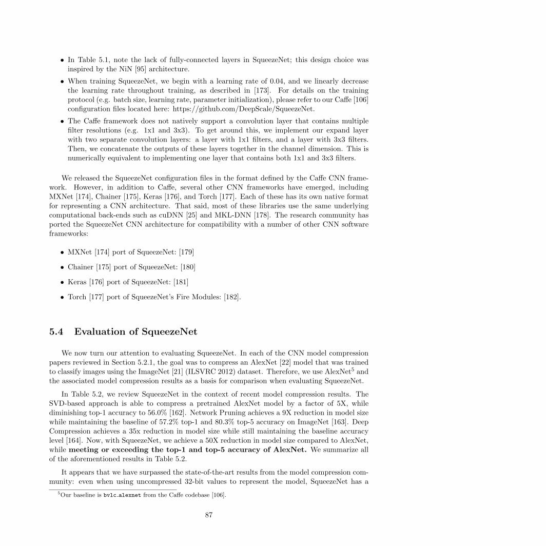
• In Table 5.1, note the lack of fully-connected layers in SqueezeNet; this design choice wasinspired by the NiN [95] architecture.

• When training SqueezeNet, we begin with a learning rate of 0.04, and we linearly decreasethe learning rate throughout training, as described in [173]. For details on the trainingprotocol (e.g. batch size, learning rate, parameter initialization), please refer to our Caffe [106]configuration files located here: https://github.com/DeepScale/SqueezeNet.

• The Caffe framework does not natively support a convolution layer that contains multiplefilter resolutions (e.g. 1x1 and 3x3). To get around this, we implement our expand layerwith two separate convolution layers: a layer with 1x1 filters, and a layer with 3x3 filters.Then, we concatenate the outputs of these layers together in the channel dimension. This isnumerically equivalent to implementing one layer that contains both 1x1 and 3x3 filters.

We released the SqueezeNet configuration files in the format defined by the Caffe CNN frame-work. However, in addition to Caffe, several other CNN frameworks have emerged, includingMXNet [174], Chainer [175], Keras [176], and Torch [177]. Each of these has its own native formatfor representing a CNN architecture. That said, most of these libraries use the same underlyingcomputational back-ends such as cuDNN [25] and MKL-DNN [178]. The research community hasported the SqueezeNet CNN architecture for compatibility with a number of other CNN softwareframeworks:

• MXNet [174] port of SqueezeNet: [179]

• Chainer [175] port of SqueezeNet: [180]

• Keras [176] port of SqueezeNet: [181]

• Torch [177] port of SqueezeNet’s Fire Modules: [182].

5.4 Evaluation of SqueezeNet

We now turn our attention to evaluating SqueezeNet. In each of the CNN model compressionpapers reviewed in Section 5.2.1, the goal was to compress an AlexNet [22] model that was trainedto classify images using the ImageNet [21] (ILSVRC 2012) dataset. Therefore, we use AlexNet5 andthe associated model compression results as a basis for comparison when evaluating SqueezeNet.

In Table 5.2, we review SqueezeNet in the context of recent model compression results. TheSVD-based approach is able to compress a pretrained AlexNet model by a factor of 5X, whilediminishing top-1 accuracy to 56.0% [162]. Network Pruning achieves a 9X reduction in model sizewhile maintaining the baseline of 57.2% top-1 and 80.3% top-5 accuracy on ImageNet [163]. DeepCompression achieves a 35x reduction in model size while still maintaining the baseline accuracylevel [164]. Now, with SqueezeNet, we achieve a 50X reduction in model size compared to AlexNet,while meeting or exceeding the top-1 and top-5 accuracy of AlexNet. We summarize allof the aforementioned results in Table 5.2.

It appears that we have surpassed the state-of-the-art results from the model compression com-munity: even when using uncompressed 32-bit values to represent the model, SqueezeNet has a

5Our baseline is bvlc alexnet from the Caffe codebase [106].

87

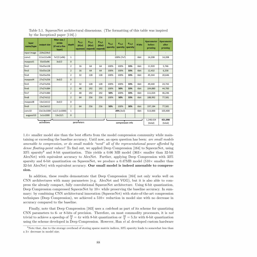
Table 5.1. SqueezeNet architectural dimensions. (The formatting of this table was inspiredby the Inception2 paper [116].)

5

layername/type outputsize

filtersize/stride

(ifnotafirelayer)

depths1x1(#1x1

squeeze)

e1x1(#1x1

expand)

e3x3(#3x3

expand)

s1x1sparsity

e1x1sparsity

e3x3sparsity

#bits#parameter

before pruning

#parameter after

pruning

inputimage 224x224x3 - -

conv1 111x111x96 7x7/2(x96) 1 6bit 14,208 14,208

maxpool1 55x55x96 3x3/2 0

fire2 55x55x128 2 16 64 64 100% 100% 33% 6bit 11,920 5,746

fire3 55x55x128 2 16 64 64 100% 100% 33% 6bit 12,432 6,258

fire4 55x55x256 2 32 128 128 100% 100% 33% 6bit 45,344 20,646

maxpool4 27x27x256 3x3/2 0

fire5 27x27x256 2 32 128 128 100% 100% 33% 6bit 49,440 24,742

fire6 27x27x384 2 48 192 192 100% 50% 33% 6bit 104,880 44,700

fire7 27x27x384 2 48 192 192 50% 100% 33% 6bit 111,024 46,236

fire8 27x27x512 2 64 256 256 100% 50% 33% 6bit 188,992 77,581

maxpool8 13x12x512 3x3/2 0

fire9 13x13x512 2 64 256 256 50% 100% 30% 6bit 197,184 77,581

conv10 13x13x1000 1x1/1(x1000) 1 6bit 513,000 103,400

avgpool10 1x1x1000 13x13/1 0

1,248,424(total)

421,098(total)

20%(3x3)

100%(7x7)

1.4× smaller model size than the best efforts from the model compression community while main-taining or exceeding the baseline accuracy. Until now, an open question has been: are small modelsamenable to compression, or do small models “need” all of the representational power afforded bydense floating-point values? To find out, we applied Deep Compression [164] to SqueezeNet, using33% sparsity6 and 8-bit quantization. This yields a 0.66 MB model (363× smaller than 32-bitAlexNet) with equivalent accuracy to AlexNet. Further, applying Deep Compression with 33%sparsity and 6-bit quantization on SqueezeNet, we produce a 0.47MB model (510× smaller than32-bit AlexNet) with equivalent accuracy. Our small model is indeed amenable to compres-sion.

In addition, these results demonstrate that Deep Compression [164] not only works well onCNN architectures with many parameters (e.g. AlexNet and VGG), but it is also able to com-press the already compact, fully convolutional SqueezeNet architecture. Using 6-bit quantization,Deep Compression compressed SqueezeNet by 10× while preserving the baseline accuracy. In sum-mary: by combining CNN architectural innovation (SqueezeNet) with state-of-the-art compressiontechniques (Deep Compression), we achieved a 510× reduction in model size with no decrease inaccuracy compared to the baseline.

Finally, note that Deep Compression [163] uses a codebook as part of its scheme for quantizingCNN parameters to 6- or 8-bits of precision. Therefore, on most commodity processors, it is nottrivial to achieve a speedup of 32

8 = 4x with 8-bit quantization or 326 = 5.3x with 6-bit quantization

using the scheme developed in Deep Compression. However, Han et al. developed custom hardware

6Note that, due to the storage overhead of storing sparse matrix indices, 33% sparsity leads to somewhat less thana 3× decrease in model size.

88

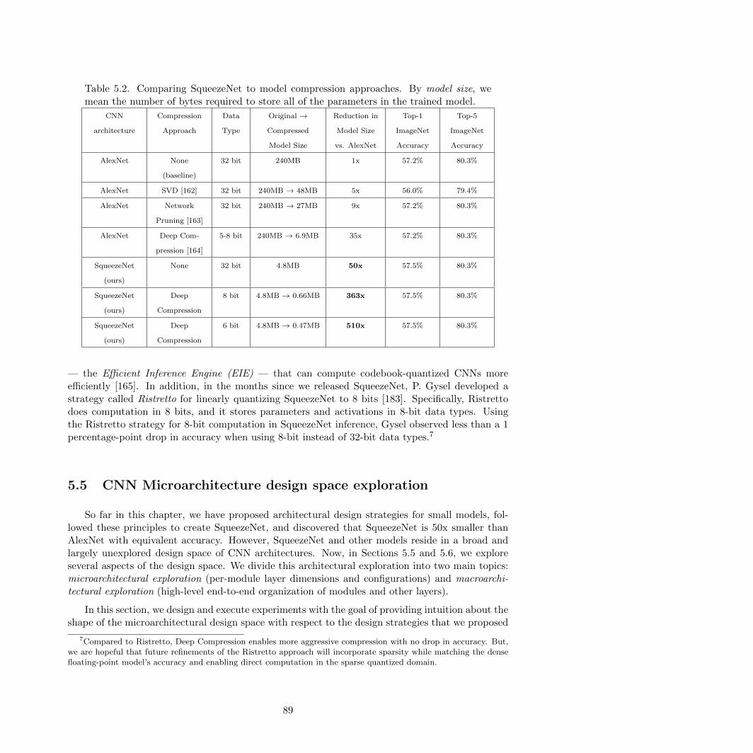
Table 5.2. Comparing SqueezeNet to model compression approaches. By model size, wemean the number of bytes required to store all of the parameters in the trained model.

CNN

architecture

Compression

Approach

Data

Type

Original →

Compressed

Model Size

Reduction in

Model Size

vs. AlexNet

Top-1

ImageNet

Accuracy

Top-5

ImageNet

Accuracy

AlexNet None

(baseline)

32 bit 240MB 1x 57.2% 80.3%

AlexNet SVD [162] 32 bit 240MB → 48MB 5x 56.0% 79.4%

AlexNet Network

Pruning [163]

32 bit 240MB → 27MB 9x 57.2% 80.3%

AlexNet Deep Com-

pression [164]

5-8 bit 240MB → 6.9MB 35x 57.2% 80.3%

SqueezeNet

(ours)

None 32 bit 4.8MB 50x 57.5% 80.3%

SqueezeNet

(ours)

Deep

Compression

8 bit 4.8MB → 0.66MB 363x 57.5% 80.3%

SqueezeNet

(ours)

Deep

Compression

6 bit 4.8MB → 0.47MB 510x 57.5% 80.3%

— the Efficient Inference Engine (EIE) — that can compute codebook-quantized CNNs moreefficiently [165]. In addition, in the months since we released SqueezeNet, P. Gysel developed astrategy called Ristretto for linearly quantizing SqueezeNet to 8 bits [183]. Specifically, Ristrettodoes computation in 8 bits, and it stores parameters and activations in 8-bit data types. Usingthe Ristretto strategy for 8-bit computation in SqueezeNet inference, Gysel observed less than a 1percentage-point drop in accuracy when using 8-bit instead of 32-bit data types.7

5.5 CNN Microarchitecture design space exploration

So far in this chapter, we have proposed architectural design strategies for small models, fol-lowed these principles to create SqueezeNet, and discovered that SqueezeNet is 50x smaller thanAlexNet with equivalent accuracy. However, SqueezeNet and other models reside in a broad andlargely unexplored design space of CNN architectures. Now, in Sections 5.5 and 5.6, we exploreseveral aspects of the design space. We divide this architectural exploration into two main topics:microarchitectural exploration (per-module layer dimensions and configurations) and macroarchi-tectural exploration (high-level end-to-end organization of modules and other layers).

In this section, we design and execute experiments with the goal of providing intuition about theshape of the microarchitectural design space with respect to the design strategies that we proposed

7Compared to Ristretto, Deep Compression enables more aggressive compression with no drop in accuracy. But,we are hopeful that future refinements of the Ristretto approach will incorporate sparsity while matching the densefloating-point model’s accuracy and enabling direct computation in the sparse quantized domain.

89

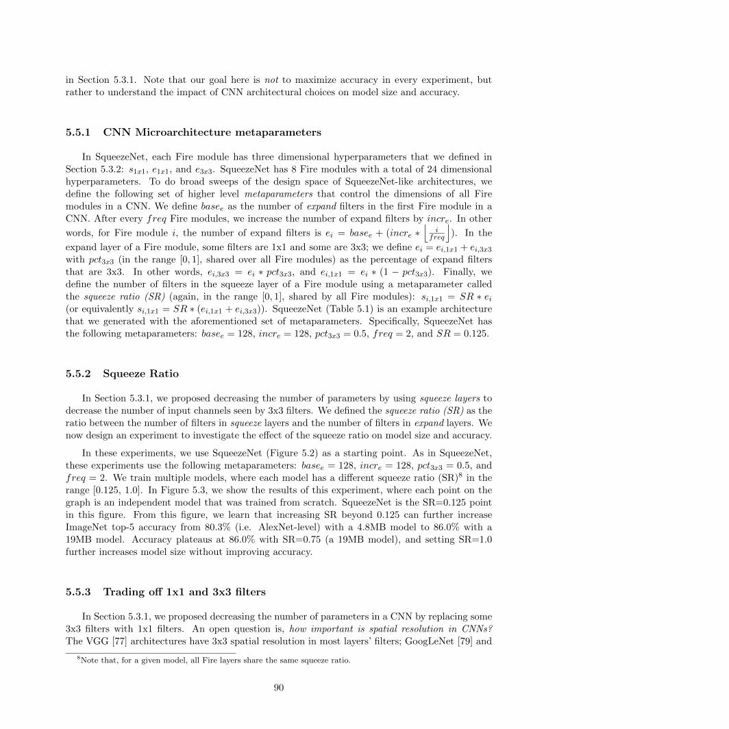
in Section 5.3.1. Note that our goal here is not to maximize accuracy in every experiment, butrather to understand the impact of CNN architectural choices on model size and accuracy.

5.5.1 CNN Microarchitecture metaparameters

In SqueezeNet, each Fire module has three dimensional hyperparameters that we defined inSection 5.3.2: s1x1, e1x1, and e3x3. SqueezeNet has 8 Fire modules with a total of 24 dimensionalhyperparameters. To do broad sweeps of the design space of SqueezeNet-like architectures, wedefine the following set of higher level metaparameters that control the dimensions of all Firemodules in a CNN. We define basee as the number of expand filters in the first Fire module in aCNN. After every freq Fire modules, we increase the number of expand filters by incre. In other

words, for Fire module i, the number of expand filters is ei = basee + (incre ∗⌊

ifreq

⌋). In the

expand layer of a Fire module, some filters are 1x1 and some are 3x3; we define ei = ei,1x1 + ei,3x3with pct3x3 (in the range [0, 1], shared over all Fire modules) as the percentage of expand filtersthat are 3x3. In other words, ei,3x3 = ei ∗ pct3x3, and ei,1x1 = ei ∗ (1 − pct3x3). Finally, wedefine the number of filters in the squeeze layer of a Fire module using a metaparameter calledthe squeeze ratio (SR) (again, in the range [0, 1], shared by all Fire modules): si,1x1 = SR ∗ ei(or equivalently si,1x1 = SR ∗ (ei,1x1 + ei,3x3)). SqueezeNet (Table 5.1) is an example architecturethat we generated with the aforementioned set of metaparameters. Specifically, SqueezeNet hasthe following metaparameters: basee = 128, incre = 128, pct3x3 = 0.5, freq = 2, and SR = 0.125.

5.5.2 Squeeze Ratio

In Section 5.3.1, we proposed decreasing the number of parameters by using squeeze layers todecrease the number of input channels seen by 3x3 filters. We defined the squeeze ratio (SR) as theratio between the number of filters in squeeze layers and the number of filters in expand layers. Wenow design an experiment to investigate the effect of the squeeze ratio on model size and accuracy.

In these experiments, we use SqueezeNet (Figure 5.2) as a starting point. As in SqueezeNet,these experiments use the following metaparameters: basee = 128, incre = 128, pct3x3 = 0.5, andfreq = 2. We train multiple models, where each model has a different squeeze ratio (SR)8 in therange [0.125, 1.0]. In Figure 5.3, we show the results of this experiment, where each point on thegraph is an independent model that was trained from scratch. SqueezeNet is the SR=0.125 pointin this figure. From this figure, we learn that increasing SR beyond 0.125 can further increaseImageNet top-5 accuracy from 80.3% (i.e. AlexNet-level) with a 4.8MB model to 86.0% with a19MB model. Accuracy plateaus at 86.0% with SR=0.75 (a 19MB model), and setting SR=1.0further increases model size without improving accuracy.

5.5.3 Trading off 1x1 and 3x3 filters

In Section 5.3.1, we proposed decreasing the number of parameters in a CNN by replacing some3x3 filters with 1x1 filters. An open question is, how important is spatial resolution in CNNs?The VGG [77] architectures have 3x3 spatial resolution in most layers’ filters; GoogLeNet [79] and

8Note that, for a given model, all Fire layers share the same squeeze ratio.

90

13#MB#of#weights#

85.3%#accuracy#

86.0%#accuracy#

19#MB#of#weights#4.8#MB#of#

weights#

80.3%#accuracy#

SqueezeNet#

Figure 5.3. Exploring the impact of the squeeze ratio (SR) on model size and ImageNetaccuracy.

Network-in-Network (NiN) [95] have 1x1 filters in some layers. In GoogLeNet and NiN, the authorssimply propose a specific quantity of 1x1 and 3x3 filters without further analysis.9 Here, we attemptto shed light on how the proportion of 1x1 and 3x3 filters affects model size and accuracy.

We use the following metaparameters in this experiment: basee = incre = 128, freq = 2,SR = 0.500, and we vary pct3x3 from 1% to 99%. In other words, each Fire module’s expand layerhas a predefined number of filters partitioned between 1x1 and 3x3, and here we turn the knob onthese filters from “mostly 1x1” to “mostly 3x3”. As in the previous experiment, these models have8 Fire modules, following the same organization of layers as in Figure 5.2. We show the results ofthis experiment in Figure 5.4. Note that the 13MB models in Figure 5.3 and Figure 5.4 are thesame architecture: SR = 0.500 and pct3x3 = 50%. We see in Figure 5.4 that the top-5 accuracyplateaus at 85.6% using 50% 3x3 filters, and further increasing the percentage of 3x3 filters leadsto a larger model size but provides no improvement in accuracy on ImageNet.

9To be clear, each filter is 1x1xChannels or 3x3xChannels, which we abbreviate to 1x1 and 3x3.

91

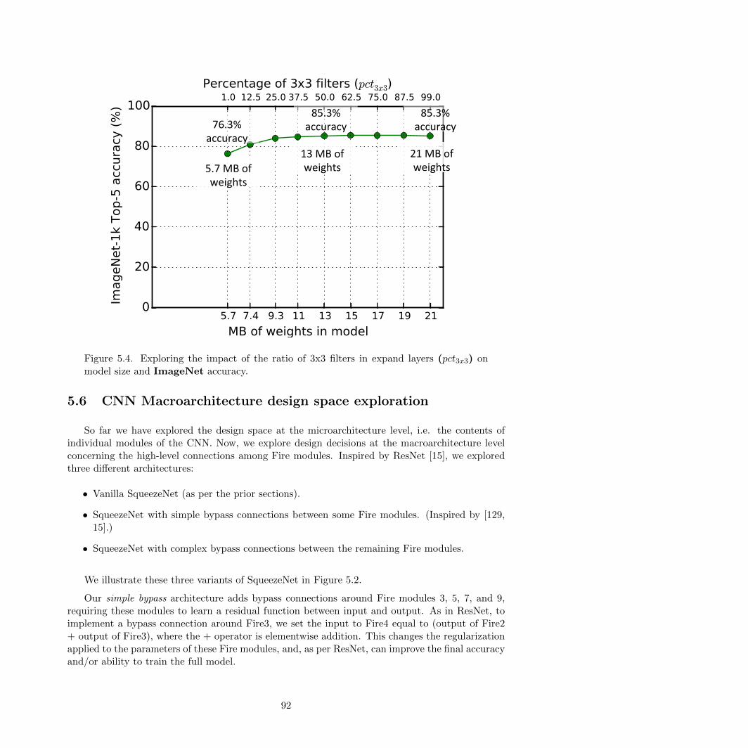
21#MB#of#weights#

13#MB#of#weights#5.7#MB#of#

weights#

85.3%#accuracy#

85.3%#accuracy#76.3%#

accuracy#

Figure 5.4. Exploring the impact of the ratio of 3x3 filters in expand layers (pct3x3) onmodel size and ImageNet accuracy.

5.6 CNN Macroarchitecture design space exploration

So far we have explored the design space at the microarchitecture level, i.e. the contents ofindividual modules of the CNN. Now, we explore design decisions at the macroarchitecture levelconcerning the high-level connections among Fire modules. Inspired by ResNet [15], we exploredthree different architectures:

• Vanilla SqueezeNet (as per the prior sections).

• SqueezeNet with simple bypass connections between some Fire modules. (Inspired by [129,15].)

• SqueezeNet with complex bypass connections between the remaining Fire modules.

We illustrate these three variants of SqueezeNet in Figure 5.2.

Our simple bypass architecture adds bypass connections around Fire modules 3, 5, 7, and 9,requiring these modules to learn a residual function between input and output. As in ResNet, toimplement a bypass connection around Fire3, we set the input to Fire4 equal to (output of Fire2+ output of Fire3), where the + operator is elementwise addition. This changes the regularizationapplied to the parameters of these Fire modules, and, as per ResNet, can improve the final accuracyand/or ability to train the full model.

92

Table 5.3. SqueezeNet accuracy and model size using different macroarchitecture configu-rations. Bold face denotes highest accuracy.

Architecture Top-1

Accuracy

Top-5

Accuracy

Model

Size

Vanilla SqueezeNet 57.5% 80.3% 4.8MB

SqueezeNet +

Simple Bypass

60.4% 82.5% 4.8MB

SqueezeNet +

Complex Bypass

58.8% 82.0% 7.7MB

One limitation is that, in the straightforward case, the number of input channels and numberof output channels has to be the same; as a result, only half of the Fire modules can have simplebypass connections, as shown in the middle diagram of Fig 5.2. When the “same number ofchannels” requirement can’t be met, we use a complex bypass connection, as illustrated on the rightof Figure 5.2. While a simple bypass is “just a wire,” we define a complex bypass as a bypassthat includes a 1x1 convolution layer with the number of filters set equal to the number of outputchannels that are needed. Note that complex bypass connections add extra parameters to themodel, while simple bypass connections do not.

In addition to changing the regularization, it is intuitive to us that adding bypass connectionswould help to alleviate the representational bottleneck introduced by squeeze layers. In SqueezeNet,the squeeze ratio (SR) is 0.125, meaning that every squeeze layer has 8x fewer output channels thanthe accompanying expand layer. Due to this severe dimensionality reduction, a limited amount ofinformation can pass through squeeze layers. However, by adding bypass connections to SqueezeNet,we open up avenues for information to flow around the squeeze layers.

We trained SqueezeNet with the three macroarchitectures in Figure 5.2 and compared theaccuracy and model size in Table 5.3. We fixed the microarchitecture to match SqueezeNet asdescribed in Table 5.1 throughout the macroarchitecture exploration. Complex and simple bypassconnections both yielded an accuracy improvement over the vanilla SqueezeNet architecture. Inter-estingly, the simple bypass enabled a higher accuracy improvement than complex bypass. Addingthe simple bypass connections yielded an increase of 2.9 percentage-points in top-1 accuracy and2.2 percentage-points in top-5 accuracy without increasing model size.

5.7 Conclusions

In this chapter, we have proposed steps toward a more disciplined approach to the design-spaceexploration of convolutional neural networks. Toward this goal we have presented SqueezeNet,a CNN architecture that has 50× fewer parameters than AlexNet and maintains AlexNet-levelaccuracy on ImageNet. We also compressed SqueezeNet to less than 0.5MB, or 510× smaller thanAlexNet without compression. Since we released this chapter as a technical report in 2016, ourcolleague Song Han and his collaborators have experimented further with SqueezeNet and modelcompression. Using a new approach called Dense-Sparse-Dense (DSD) [184], Han et al. use model

93

compression during training as a regularizer to further improve accuracy, producing a compressedset of SqueezeNet parameters that is 1.2 percentage-points more accurate on ImageNet-1k, andalso producing an uncompressed set of SqueezeNet parameters that is 4.3 percentage-points moreaccurate, compared to our results in Table 5.2.

In the context of this chapter, we focused on ImageNet as a target dataset. However, it hasbecome common practice to apply ImageNet-trained CNN representations to a variety of appli-cations such as fine-grained object recognition [54, 185], logo identification in images [55], andgenerating sentences about images [57]. ImageNet-trained CNNs have also been applied to a num-ber of applications pertaining to autonomous driving, including pedestrian and vehicle detection inimages [47, 48, 56] and videos [186], as well as segmenting the shape of the road [187]. We thinkSqueezeNet will be a good candidate CNN architecture for a variety of applications, especiallythose in which small model size is of importance. In fact, since the original publication of theSqueezeNet techncial report [18], we have done follow-on work — SqueezeDet [188] — which buildsupon SqueezeNet to address the problem of localized object detection. As of December 2016, theSqueezeDet models define the state-of-the-art results for accuracy, model size, and frame rate onthe KITTI [68] object detection dataset.

SqueezeNet is one of several new CNNs that we have discovered while broadly exploring thedesign space of CNN architectures. We hope that SqueezeNet will inspire the reader to considerand explore the broad range of possibilities in the design space of CNN architectures and to performthat exploration in a more systematic manner.

94

Chapter 6

Conclusions

6.1 Contributions

CNN/DNN models have become the best approach for solving a variety of problems in the text,audio, and visual domains with unprecedented accuracy. Among these domains, visual (e.g. imagesand video) applications are often the most computationally-intensive use-cases of CNN/DNNs. Inthe interest of choosing the most challenging and computationally-intensive problems, we focusedthis dissertation primarily on the application of CNNs to visual recognition applications.

Even within a specific domain (e.g. images), there does not appear to be a single “best”CNN architecture that is ideal for all computer vision problems under all possible constraints onaccuracy, energy-efficiency, and other metrics. Further, CNNs comprise an enormous design space.1

Each architecture in the CNN design space presents its own tradeoffs in terms of computationalrequirements, communication overhead during distributed training, energy-efficiency, accuracy onthe problem at hand, and so on. The CNN design space is not the first large design space thatcomputer scientists have explored. The design space of computer processor hardware architecturesis an example of an other large and complex design space.

The MESCAL book [34] codified a number best practices or “themes” for exploring the designspace of computational hardware architectures. We drew inspiration from the MESCAL book inhow we organized this dissertation on exploring the design space of CNN architectures. Quitesimilar to the MESCAL themes, our four themes are:

• Comprehensively defining benchmarks and metrics. (Chapter 2)

• Rapidly training CNN/DNNs. (Chapter 3)

• Defining and describing the CNN/DNN design space. (Chapter 4)

• Exploring the design space of CNN/DNN architectures. (Chapter 5)

1As we learned in Section 4.7, just a small region of the CNN design space comprises approximately 30 billiondifferent CNN architectures.

95

Taken together, these themes comprise a methodology that will enable the reader to explore theCNN design space in a systematic and directed way.

In the following sections, we review our key findings on each of the four themes.

6.1.1 Comprehensively defining benchmarks and metrics

CNN/DNNs comprise an enormous design space. Therefore, when exploring the CNN/DNNdesign space, if you don’t know what you’re looking for, you’re unlikely to find it. With this in mind,it’s useful to define clear goals in terms of benchmarks and metrics. Benchmarks (e.g. datasets)should be representative of the target application. For example, if the goal is to recognize vehicleson the road, then the training and testing data should include annotated road scenes. Importantmetrics include not only accuracy, but also quantity of computation, quantity of communication,latency, energy-efficiency, and so on.

When building a deployable and highly efficient CNN-based system, it is sensible to bringtogether a CNN architecture team, a software architecture team, and a hardware architecture team.To measure individual teams’ contributions, the CNN team can be evaluated on the quantity ofcomputation and accuracy, and the hardware team can be evaluated on power consumption andbest-case peak throughput. While hardware and CNNs can be evaluated individually, it is difficultto evaluate the software team’s contributions in isolation. To evaluate the whole organization’sprogress toward an efficient full-stack solution, it is useful to measure metrics such as energy-efficiency and speed.

6.1.2 Rapidly training CNN/DNNs

Long training times impose a severe limitation on progress in deep neural network research andproductization. Accelerating CNN training has several benefits. First, faster CNN training enablesmodels to be trained on ever-increasing dataset sizes in a tractable amount of time. AcceleratingCNN training also enables product teams to bring CNN-based products to market more rapidly.These and other compelling applications led us to focus on the problem of accelerating CNNtraining, and our work has culminated in the FireCaffe distributed CNN training system. WithFireCaffe, we achieved a 47x speedup when training the GoogLeNet model. This enabled us totrain GoogLeNet in 10.5 hours on 128 GPUs instead of 3 weeks on 1 GPU. After achieving thisresult, we turned our attention to identifying, training, and evaluating new CNN architectures withspecific goals in mind. The use of FireCaffe’s rapid training functionality enabled us to productivelyexplore the design space of CNNs with minimal turnaround time for each experiment.

6.1.3 Defining and describing the CNN/DNN design space

The CNN/DNN architecture defines the quantity of computation that is required per datasample during both training and inference. In the context of a CNN-based system, the CNNarchitecture impacts most of the key metrics, including accuracy, quantity of computation, quantityof communication, latency, energy-efficiency, and model size. Therefore, when preparing to explorethe design space of CNN architectures, it is useful to first understand how the design of the CNN

96

architecture impacts some of these metrics. Surprisingly, after conducting a literature survey, wewere not able to find a practical guide on how the design of the CNN architecture impacts thebehavior (e.g. quantity of computation, quantity of communication) of a CNN-based system. Toaddress this, we developed a guide that explains how we reason about these design choices.

When looking at a CNN architecture, it can be a bit intimidating to reason about how eachpotential change to the CNN would affect metrics such as the quantity of computation. However,we found that most changes to a CNN architecture produces one of the following effects:

• A local change to a layer in a deep CNN typically has little impact on the CNN’s total quantityof computation.

• A global change to layer Li affects all layers downstream of Li and can have a multiplicativeeffect on the CNN’s total quantity of computation.

To date, we have not seen intuition like this written down anywhere, and this motivated us to explainour intuition and analysis of the topic. Better understanding of CNN architectural dimensionsshould enable the reader to reason more clearly about the region of the design space that he or shewould like to explore.

6.1.4 Exploring the design space of CNN/DNN architectures

With of all of the aforementioned information in place, we were able to put our design-spaceexploration methodology into practice. We set out the following challenge for ourselves: Producesmall models (i.e. models with few parameters) that achieve competitive accuracy on a computervision benchmark. In this challenge problem, the benchmark is the ImageNet-1k image classificationdataset [21], and the metrics are accuracy and model size. As a bonus, small models can betrained at larger scale using distributed data-parallel training, and this enabled us to conduct ourexploration more quickly. We chose benchmarks (accuracy and model size) that are independent ofthe choice of hardware and software for executing the CNN. However, as we will see in Section 6.3,other teams have since adapted our small models to achieve system-level goals such as developingFPGA-based CNN systems in which the CNN model fits entirely on-chip.

Early on in this process, we first defined a region of the design space to explore. We did ourbest to define a region of the design space that is likely to contain small models — e.g. CNN designsthat use Fire modules, which make abundant use of 1x1 filters, and they alternate between manyand few filters per layer. Within this design space, we identified SqueezeNet, a model that has 50xfewer parameters than AlexNet but achieves AlexNet-level accuracy on the ImageNet-1k dataset.Further, by applying model compression to SqueezeNet, we obtained a model that is 510x smallerthan AlexNet but produces AlexNet-level accuracy on ImageNet-1k.

97

6.2 Impact of our FireCaffe work on accelerating CNN/DNN

training

Much of the content in this dissertation (Chapters 1, 2, 4, and 6) is being published for the firsttime in these pages. Meanwhile, we published versions of Chapters 3 and 5 within the last twelvemonths [17, 18]. Despite the fact that we only recently released these publications, this work hasbegun to make an impact on the CNN research literature.

As we learned in Chapter 3, it is common for CNNs to take multiple weeks to train on asingle GPU. The slow turnaround time of CNN training impedes progress in CNN research andproductization. Therefore, over the last couple of years, distributing CNN training over multipleprocessors has become an increasingly active area of research. Retrospectively, it appears that therelease of our FireCaffe paper in late 2015 and its subsequent publication in CVPR 2016 may havebeen a turning point in how researchers have approached distributed CNN training problems.

6.2.1 Before FireCaffe

In early 2015, prior to embarking on the development of the FireCaffe, we surveyed the literatureon distributed CNN/DNN training. In the course of this literature survey, we observed the followingtrends.

• Parallelism strategies. In the papers published prior to 2016, researchers experimentedwith a range of parallelism strategies. Model parallelism was a staple of many of these papers,such as those from Microsoft [107], Google [108], and CMU [189]. Researchers from Stanfordand NVIDIA even designed a CNN architecture that was optimized for model parallel trainingon a cluster of GPUs [190].2

• Communication paradigms. Many of the research papers assumed (either explicitly orimplicitly) that that it was manifest destiny that some variant of asynchronous communicationwould emerge as the best choice. These papers include HOGwild [191] and its follow-onworks [192, 193], as well as work from Microsoft [107] and Google [108].

• Evaluation metrics. Researchers used a wide range of metrics to evaluate their work. But,one common metric was number of processors utilized. For example, the DistBelief paperfrom Google [108] and the Deep Image paper from Baidu [111] each reported the number ofprocessors used, but it was difficult to interpret these results because each of these papersused a proprietary dataset and reported time-to-convergence only on that dataset. As we willsee in the next subsection, recent works have done this type of evaluation on publicly-availabledatasets, which makes it easier to make comparisons between the different approaches.

• Hardware communication networks. The early papers tended to place little emphasison the choice of networking hardware used to communicate between servers. In some papers,using slow (e.g. 1 Gbps Ethernet) connections between servers led to severe limitationson the speed and scalability of the system as a whole [194]. In other papers, the authors

2To be clear, this CNN architecture used the natural data parallelism within each GPU, but it used modelparallelism as the primary mechanism for scaling over multiple GPUs.

98

simply focused on scaling the training CNN/DNN models over multiple GPUs within a singleserver [103, 105, 120, 121, 122, 195].

6.2.2 Since FireCaffe

Compared to the approaches mentioned in the previous subsection, our work in the FireCaffepaper [17] (reproduced in Chapter 3 of this dissertation) advocated for the following: (a) data par-allelism, (b) synchronous communication, (c) evaluation of time-to-convergence to a predeterminedaccuracy level on a publicly-available dataset, and (d) using the fastest communication hardwareavailable. We were early pioneers of these approaches; in research papers on distributed CNN/DNNtraining that have been released in the last few months, we’ve noticed the following trends emerge:

• Parallelism strategy: focus on data parallelism. In our FireCaffe paper [17], we extolledthe benefits of focusing on data parallel communication in distributed CNN training. Inthe papers published in 2016, researchers have gravitated toward data-parallel training ofCNNs. Perhaps most interestingly, the Google Brain team — which was an advocate formodel parallelism in its earlier paper [108] — recently used data parallelism (without modelparallelism) in the distributed CNN training results that they released at ICLR 2016 [196].

• Communication paradigm: synchronous. In our FireCaffe paper [17], we demonstratedthat the limiting factor in asynchronous communication is typically the need for a centralparameter server. To mitigate this, we advocated for synchronous communication, whichenables the use of collective communication approaches such as reduction trees. While theparameter server slows down linearly in the number of workers (e.g. GPU workers), collectivecommunication slows down logarithmically in the number of workers, enabling it to run effi-ciently at larger scale. This approach has begun to take hold in the recent research literature.Intel recently published their latest results on distributed CNN training to 256 servers, andthe communication is fully synchronous [178]. Incidentally, a key individual at Intel told usthat the FireCaffe paper was used “as a bible” by the Intel teams who were in charge ofproducing these results [197]. Further, a version of the Theano CNN/DNN framework thatsupports synchronous data-parallel communication was released in mid-2016 [198]. Finally,the recent paper from Google used fully-synchronous communication for distributed CNNtraining, and it even provided an approach to more elegantly address fault tolerance in thesynchronous communication paradigm [196].

• Evaluation metric: time to convergence. In our FireCaffe paper [17], we advocated forthe following strategy for evaluating a distributed CNN training approach. Given a specificdataset and a specific target accuracy level, the goal is to train a CNN to the desired accuracylevel as rapidly as possible. Everything else is up to the system architect: the choice of CNNarchitecture, the choice of computational hardware, the choice of communication hardware,and so on. This benchmarking methodology appears to be catching on. Recent papers fromIntel [178] and Google [196] use this methodology in their benchmarking.

• Hardware communication network: 56 Gbit/s or better. In our FireCaffe paper [17],we encouraged system architects to use the fastest communication hardware that is availableto them. Universities and large corporations sometimes have datacenters containing a numberof different compute clusters. For employees who are deciding which of their existing compute

99

clusters to use for distributed CNN/DNN training, our approach would encourage them touse the compute cluster that has the fastest network connections (e.g. 40 Gbit/s ethernetor 56 Gbit/s Infiniband) bridging the servers in the cluster. If designing or ordering newcompute clusters, our approach would encourage the system infrastructure team to spenda substantial portion of the budget to purchase fast communication hardware. Our way ofthinking appears to be catching on. In their recent distributed CNN training results, Intelused 56 Gbit/s FDR Infiniband network hardware when scaling to 256 CPU servers [178].3

6.2.3 Future work: Further improvements to distributed CNN/DNN training

As we discussed in Chapter 3, in order to distribute the training of a CNN/DNN model overmultiple servers, it is necessary to communicate among the servers during the training process. Inthe applications described in the general literature on distributed computing, the need for commu-nication among servers is quite common. In the distributed computing literature, the software opti-mization of overlapping communication and computation has been studied for more than twenty-fiveyears [201, 202].

In our FireCaffe results, we did not overlap communication and computation. That is, if traininga particular CNN on a particular hardware platform requires a total of 5 hours of communicationand 5 hours of computation, our FireCaffe results would say “the CNN took 10 hours to train.”However, the Purine [203] multi-GPU CNN training framework proposed a form of communication-computation overlapping. The basic idea is as follows. In the backward pass, whenever a layer Li

finishes computing its data gradients (∇Di), Purine would stage these gradients for communication.However, these gradients will not be needed until it is time to compute the forward pass of Li, andthis allows for ∇Di to be communicated while computation is performed on other layers. Let usconsider the best-case speedup when applying this approach. In the best case, we would have aCNN where all layers had exactly the same amount of communication (e.g. 1MB of data) andexactly the same amount of computation (e.g. 10 GFLOPs per batch). In the best case scenario,the time to communicate (in the form of an allreduce sum) 1MB of data over all servers is identicalto the time required to perform 10 GFLOPs of computation on one server. In this ideal case, theoverlapping approach described in Purine [203] would lead to precisely a 2x speedup over non-overlapping training. However, in all of the CNNs described in this dissertation (e.g. Tables 4.2—4.8, Table 5.1), there are substantially more parameters (in bytes) in the final layers than in the earlylayers, and layers vary in their computational requirements (in FLOPs). Given that these practicalcases deviate from the “best case scenario” that we described, overlapping communication andcomputation would lead to less than a 2x speedup over serialized communication and computation.That said, there is an opportunity to address this by designing CNN architectures that exposemore overlapping opportunities by making the layers more homogenous in their communicationand computation requirements.

3Note that, while many researchers have struggled to implement CNNs efficiently on CPUs (e.g. [199], [200]), wehave found that it’s possible to achieve on the order of 1 TFLOP/s per CPU when executing CNNs using well-tunedimplementations.

100

6.3 Impact of our work on exploring the design space of CNN

architectures

The last four years have marked a resurgence in the use of neural networks for computer vision,led chiefly by the unprecedented accuracy that modern deep neural networks provide. In thisfrenzy, hardware architects have developed a variety of accelerators and computational platformstargeted specifically at CNN/DNNs. We have observed a recurring theme in this work: A teamof hardware architects begin by taking off-the-shelf CNN architecture such as AlexNet [22], andthen they engineer an accelerator designed with this off-the-shelf model in mind. In fact, all of thefollowing work on FPGA- and ASIC-based CNN accelerators reports its speed and efficiency resultssolely on the AlexNet CNN architecture: Eyeriss [204], ShiDianNao [205], Motamedi et al. [206],Ovtcharov et al. [92], and Zhang et al. [207]. There is certainly merit in comparing the efficiencyof different computational hardware approaches on the same CNN architecture. However, in their2012 paper Krizhevsky et al. were quite clear that the AlexNet model was designed to leverageproblem sizes that are ideal for an NVIDIA GTX580 GPU [22]. When using other computationalhardware — and especially when designing new hardware — it is critical to design CNNs that willexecute efficiently on this hardware. In other words, to achieve the best possible results on variousmetrics (e.g. accuracy, throughput, energy-efficiency), it is ideal to co-design the CNN architecture,the software implementation, and the computational hardware.

Encouragingly, researchers have begun to make progress on holistically designing CNN architec-tures, software, and hardware. One problem that we mentioned in Chapter 5 is that the parametersof large CNNs such as AlexNet [22] typically do not fit on-chip in today’s processors or FPGAs,requiring time- and energy-intensive communication with off-chip DRAM. Building on their pre-vious work in Deep Compression [164], Han et al. recently developed Efficient Inference Engine(EIE) [165]. EIE is an accelerator that is able to retain compressed versions of AlexNet [22] orVGG-19 [77] in on-chip SRAMs, dramatically reducing the need for off-chip memory traffic. Whilemost CNN accelerators process dense representations of the parameters and data, EIE operatesdirectly on the sparse representation of the CNN that is produced by Deep Compression. The EIEauthors point out that the use of models such as SqueezeNet (with or without compression) furtherreduces the memory requirements.

Our work has begun to directly impact how researchers co-design CNNs and hardware. D.Gschwend recently released a report and implementation of ZynqNet, which comprises custom CNNsand a custom hardware implementation for executing CNN inference on Xilinx Zynq FPGAs [208].In his report, Gschwend says, “[We used] SqueezeNet as the basis for our own CNN topology, dueto its good fit for an FPGA-based implementation. The tiny parameter set could even be fit intothe on-chip SRAM of a medium-sized FPGA, and optimizations are relatively easy to try thanks tothe fast training cycles and the clear network structure.” Rather than simply porting SqueezeNetto his FPGA accelerator, Gschwend used SqueezeNet as a starting point for developing his own“ZynqNet” family of CNN architectures. With the goal of efficiently targeting FPGAs, Gschwendoutlined four particular CNN design objectives to be used in the ZynqNet CNN architectures:4

4While Gschwend argues that these design objectives are particularly critical for enabling straightforward andefficient FPGA implementations, the objectives may also enable more efficient execution on other hardware such asCPUs and GPUs.

101

1. Constrain the model size so that the CNN’s parameters will fit into an FPGA’s on-chipmemory.

2. Use power-of-two sizes wherever possible in CNN dimensions. Gschwend mentions that, “Onthe FPGA, multiplications and divisions by a power of 2 can be calculated with inexpen-sive shift operations, which enables optimizations in the addressing of image caches in theaccelerator.”

3. For downsampling the activations produced by CNN layers, replace max-pooling with stridedconvolution wherever possible (inspired by [209]). Not only does this eliminate the need toconsume chip-area with max-pooling hardware, but Gschwend found situations where thisimproves accuracy on ImageNet-1k image classification.

4. Equalize the quantity of activations, or “layer capacity,” produced by each module in theCNN. This helps to further conserve memory space on the FPGA. In addition, Gschwendfound cases where this change also leads to higher accuracy.

All of this culminates in a CNN architecture that Gschwend was able to implement on an FPGA.Beyond the opportunities for improving speed and efficiency, it appears that co-designing theCNN architecture with FPGA hardware implementation actually saved Gschwend a substantialamount of engineering effort. In an appendix of Gschwend’s report, it mentions that all the workmentioned above was developed by Gschwend on his own during a 6-month Master’s thesis project.Contrast that with Eyeriss [204] and ShiDianNao [205], where each group of authors spent multipleyears with a team of five to ten engineers to develop and optimize hardware architectures forAlexNet. Gschwend’s work demonstrates that designing the “right” CNN architecture can lead toa substantial savings in hardware-engineering effort. Works such as EIE [165] and ZynqNet [208]are encouraging, and we anticipate that orders-of-magnitude improvements remain on the table inseveral key metrics (e.g. energy-efficiency, throughput) for those who choose to co-design the CNNarchitecture, software, and hardware.

102

Bibliography

[1] Jordan Boyd-Graber and Philip Resnik, “Holistic sentiment analysis across languages: Mul-tilingual supervised latent dirichlet allocation,” in Empirical Methods in Natural LanguageProcessing (EMNLP), 2010.

[2] W. Naptali, M. Tsuchiya, and S. Nakagawa, “Topic dependent class based language modelevaluation on automatic speech recognition,” in IEEE Spoken Language Technology Workshop(SLT), 2010.

[3] Jike Chong, Ekaterina Gonina, and Kurt Keutzer, “Efficient automatic speech recognitionon the gpu,” in GPU Computing Gems Emerald Edition, 2011.

[4] Xiaodan Zhuang, Stavros Tsakalidis, Shuang Wu, Pradeep Natarajan, Rohit Prasad, andPrem Natarajan, “Compact audio representation for event detection in consumer media,” inINTERSPEECH, 2012.

[5] B. Elizalde, H. Lei, and G. Friedland, “An i-vector representation of acoustic environmentsfor audio-based video event detection on user generated content,” in IEEE InternationalSymposium on Multimedia (ISM), 2013.

[6] Pedro F. Felzenszwalb, Ross B. Girshick, David McAllester, and Deva Ramanan, “Objectdetection with discriminatively trained part-based models,” PAMI, 2010.

[7] Joao Carreira, Rui Caseiro, Jorge Batista, and Cristian Sminchisescu, “Semantic segmen-tation with second-order pooling,” in European Conference on Computer Vision (ECCV),2012.

[8] F. Perronnin and J. Sanchez, “Compressed fisher vectors for LSVRC,” in PASCAL VOC /ImageNet Workshop at ICCV, 2011.

[9] Ozan Irsoy and Claire Cardie, “Deep recursive neural networks for compositionality in lan-guage,” in NIPS, 2014.

[10] Tomas Mikolov, Ilya Sutskever, Kai Chen, Greg Corrado, and Jeffrey Dean, “Distributedrepresentations of words and phrases and their compositionality,” in NIPS, 2013.

[11] Dario Amodei, Rishita Anubhai, Eric Battenberg, Carl Case, Jared Casper, Bryan C. Catan-zaro, Jingdong Chen, Mike Chrzanowski, Adam Coates, Greg Diamos, Erich Elsen, JesseEngel, Linxi Fan, Christopher Fougner, Tony Han, Awni Y. Hannun, Billy Jun, PatrickLeGresley, Libby Lin, Sharan Narang, Andrew Y. Ng, Sherjil Ozair, Ryan Prenger, Jonathan

103

Raiman, Sanjeev Satheesh, David Seetapun, Shubho Sengupta, Yi Wang, Zhiqian Wang,Chong Wang, Bo Xiao, Dani Yogatama, Jun Zhan, and Zhenyao Zhu, “Deep speech 2:End-to-end speech recognition in english and mandarin,” arXiv:1512.02595, 2015.

[12] Khalid Ashraf, Benjamin Elizalde, Forrest Iandola, Matthew Moskewicz, Julia Bernd, GeraldFriedland, and Kurt Keutzer, “Audio-based multimedia event detection with dnns and sparsesampling,” in ICMR, 2015.

[13] Shaoqing Ren, Kaiming He, Ross Girshick, and Jian Sun, “Faster r-cnn: Towards real-timeobject detection with region proposal networks,” in NIPS, 2015.

[14] Jonathan Long, Evan Shelhamer, and Trevor Darrell, “Fully convolutional networks forsemantic segmentation,” in CVPR, 2015.

[15] Kaiming He, Xiangyu Zhang, Shaoqing Ren, and Jian Sun, “Deep residual learning for imagerecognition,” arXiv:1512.03385, 2015.

[16] Mark Everingham, Luc Van Gool, Christopher K. I. Williams, John Winn, and AndrewZisserman, “The pascal visual object classes (voc) challenge,” International Journal ofComputer Vision (IJCV), 2010.

[17] Forrest N. Iandola, Khalid Ashraf, Matthew W. Moskewicz, and Kurt Keutzer, “FireCaffe:near-linear acceleration of deep neural network training on compute clusters,” in CVPR,2016.

[18] Forrest N. Iandola, Song Han, Matthew W. Moskewicz, Khalid Ashraf, William J. Dally, andKurt Keutzer, “SqueezeNet: Alexnet-level accuracy with 50x fewer parameters and <0.5mbmodel size,” arXiv:1602.07360, 2016.

[19] Matthew W. Moskewicz, Forrest N. Iandola, and Kurt Keutzer, “Boda-RTC: Productivegeneration of portable, efficient code for convolutional neural networks on mobile computingplatforms,” arXiv:1606.00094, 2016.

[20] Jason Yosinski, Jeff Clune, Yoshua Bengio, and Hod Lipson, “How transferable are featuresin deep neural networks?,” in NIPS, 2014.

[21] J. Deng, W. Dong, R. Socher, L.-J. Li, K. Li, and L. Fei-Fei, “ImageNet: A large-scalehierarchical image database,” in CVPR, 2009.

[22] Alex Krizhevsky, Ilya Sutskever, and Geoffrey E. Hinton, “ImageNet Classification with DeepConvolutional Neural Networks,” in NIPS, 2012.

[23] Anting Shen, “BeaverDam: Video annotation tool for computer vision training labels,” M.S.thesis, University of California, Berkeley, 2016.

[24] Anting Shen, “BeaverDam,” https://github.com/antingshen/beaverdam, 2016.

[25] Sharan Chetlur, Cliff Woolley, Philippe Vandermersch, Jonathan Cohen, John Tran,Bryan Catanzaro, and Evan Shelhamer, “cuDNN: efficient primitives for deep learning,”arXiv:1410.0759, 2014.

[26] Matthew W. Moskewicz, Ali Jannesari, and Kurt Keutzer, “A metaprogramming and auto-tuning framework for deploying deep learning applications,” arXiv:1611.06945, 2016.

104

[27] P. van Zeijl, J. W. T. Eikenbroek, P. P. Vervoort, S. Setty, J. Tangenherg, G. Shipton,E. Kooistra, I. C. Keekstra, D. Belot, K. Visser, E. Bosma, and S. C. Blaakmeer, “Abluetooth radio in 0.18- mu;m cmos,” IEEE Journal of solid-state circuits, 2002.

[28] Rob Munoz, “Asics vs. net processors: Understanding the true costs,” http://www.eetimes.

com/document.asp?doc_id=1277605, 2002.

[29] “List of bitcoin mining asics,” 2016, https://en.bitcoin.it/wiki/List_of_Bitcoin_

mining_ASICs.

[30] L. Codrescu, W. Anderson, S. Venkumanhanti, M. Zeng, E. Plondke, C. Koob, A. Ingle,C. Tabony, and R. Maule, “Hexagon dsp: An architecture optimized for mobile multimediaand communications,” IEEE Micro, 2014.

[31] T. Chen, Z. Du, N. Sun, J. Wang, C. Wu, Y. Chen, and O. Temam, “High-throughputaccelerator for ubiquitous machine-learning,” in International Conference on ArchitecturalSupport for Programming Languages and Operating Systems (ASPLOS), 2014.

[32] “Nvidia geforce gtx 980. featuring maxwell, the most advanced gpu ever made,” NVIDIAWhitepaper, 2014.

[33] M. Hempstead, D. Brooks, and G. Y. Wei, “An accelerator-based wireless sensor networkprocessor in 130 nm cmos,” IEEE Journal on Emerging and Selected Topics in Circuits andSystems, 2011.

[34] Matthias Gries and Kurt Keutzer, Building ASIPs: The Mescal Methodology, Springer, 2005.

[35] Forrest Iandola and Michael Syphers, “Electron beam focusing for the international linearcollider,” in American Association for the Advancement of Science Annual Meeting (AAAS),2008.

[36] Forrest N. Iandola, Matthew O’Brien, and Richard Procassini, “PyMercury: interactivepython for the mercury monte carlo particle transport code,” in International Conferenceon Mathematics and Computational Methods Applied to Nuclear Science and Engineering(M&C), 2011.

[37] Forrest N. Iandola, Jan Schuemann, Jungwook Shin, Bruce Faddegon, Harald Paganetti, andJoseph Perl, “Representing range compensators in the TOPAS monte carlo system,” inEuropean Workshop on Monte Carlo Treatment Planning (MCTP), 2012.

[38] Vivek Kini, Forrest Iandola, and Timothy Murray, “Techniques for assigning priorities tostreams of work,” US Patent Number 20140344822, 2014.

[39] Forrest Iandola, Fatemeh Saremi, Tarek Abdelzaher, Praveen Jayachandran, and Aylin Yener,“Real-time capacity of networked data fusion,” in International Conference on InformationFusion, 2011.

[40] Fatemeh Saremi, Praveen Jayachandran, Forrest Iandola, Yusuf Sarwar, and Tarek Abdelza-her, “On schedulability and time composability of multisensor data aggregation networks,”in International Conference on Information Fusion, 2012.

105

[41] Steena Monteiro, Forrest Iandola, and Daniel Wong, “STOMP: Statistical techniques foroptimizing and modeling performance of blocked sparse matrix vector multiplication,” in In-ternational Symposium on Computer Architecture and High Performance Computing (SBAC-PAD), 2016.

[42] Mehdi Maasoumy, Pierluigi Nuzzo, Forrest Iandola, Maryam Kamgarpour, AlbertoSangiovanni-Vincentelli, and Claire Tomlin, “Optimal load management system for aircraftelectric power distribution,” in IEEE Conference on Decision and Control (CDC), 2013.

[43] Mahsa Kamali, Ido Omer, Forrest Iandola, Eyal Ofek, and John C. Hart, “Linear clutterremoval from urban panoramas,” in ISVC, 2011.

[44] Mahsa Kamali, Forrest N. Iandola, Hui Fang, and John C. Hart, “Methmorph: Simulatingfacial deformation due to methamphetamine usage,” in ISVC, 2011.

[45] Michael Anderson, Forrest Iandola, and Kurt Keutzer, “Quantifying the energy efficiency ofobject recognition and optical flow,” UC Berkeley Technical Report, 2014.

[46] Forrest N. Iandola, Matthew W. Moskewicz, and Kurt Keutzer, “libHOG: Energy-efficienthistogram of oriented gradient computation,” in ITSC, 2015.

[47] Forrest N. Iandola, Matthew W. Moskewicz, Sergey Karayev, Ross B. Girshick, Trevor Dar-rell, and Kurt Keutzer, “Densenet: Implementing efficient convnet descriptor pyramids,”arXiv:1404.1869, 2014.

[48] Ross B. Girshick, Forrest N. Iandola, Trevor Darrell, and Jitendra Malik, “Deformable partmodels are convolutional neural networks,” in CVPR, 2015.

[49] Bor-Yiing Su, Parallel Application Library for Object Recognition, Chapter 3, Ph.D. thesis,University of California, Berkeley, 2012.

[50] Forrest N. Iandola, David Sheffield, Michael Anderson, Phitchaya Mangpo Phothilimthana,and Kurt Keutzer, “Communication-minimizing 2d convolution in gpu registers,” in ICIP,2013.

[51] Forrest N. Iandola, David Sheffield, Michael Anderson, Phitchaya Mangpo Phothilimthana,and Kurt Keutzer, “Minimizing memory communication for 2d image convolution in gpuregisters,” in GPU Technology Conference (GTC), 2013.

[52] “NVIDIA Performance Primitives (NPP),” developer.nvidia.com/npp.

[53] Matthew W. Moskewicz, “Boda: A c++ framework for efficient experiments in computervision,” https://github.com/moskewcz/boda, 2016.

[54] Ning Zhang, Ryan Farrell, Forrest Iandola, and Trevor Darrell, “Deformable part descriptorsfor fine-grained recognition and attribute prediction,” in ICCV, 2013.

[55] Forrest N. Iandola, Anting Shen, Peter Gao, and Kurt Keutzer, “DeepLogo: Hitting logorecognition with the deep neural network hammer,” arXiv:1510.02131, 2015.

[56] Khalid Ashraf, Bichen Wu, Forrest N. Iandola, Matthew W. Moskewicz, and Kurt Keutzer,“Shallow networks for high-accuracy road object-detection,” arXiv:1606.01561, 2016.

106

[57] Hao Fang, Saurabh Gupta, Forrest Iandola, Rupesh Srivastava, Li Deng, Piotr Dollar, Jian-feng Gao, Xiaodong He, Margaret Mitchell, John C. Platt, C. Lawrence Zitnick, and GeoffreyZweig, “From captions to visual concepts and back,” in CVPR, 2015.

[58] Peter Jin, Forrest Iandola, and Kurt Keutzer, “How to scale distributed deep learning?,” inNIPS MLSys Workshop, 2016.

[59] John Canny, Huasha Zhao, Ye Chen, Bobby Jaros, and Jiangchang Mao, “Machine learningat the limit,” in IEEE International Conference on Big Data, 2015.

[60] Christopher Cieri, David Miller, and Kevin Walker, “The fisher corpus: a resource for thenext generations of speech-to-text,” in International Conference on Language Resources andEvaluation (LREC), 2004.

[61] Sergio Guadarrama, “BVLC googlenet,” https://github.com/BVLC/caffe/tree/master/

models/bvlc_googlenet, 2015.

[62] Andrej Karpathy, George Toderici, Sanketh Shetty, Thomas Leung, Rahul Sukthankar, andLi Fei-Fei, “Large-scale video classification with convolutional neural networks,” in CVPR,2014.

[63] Douglas B. Paul and Janet M. Baker, “The design for the wall street journal-based csrcorpus,” in Association for Computational Linguistics Workshop on Speech and NaturalLanguage, 1992.

[64] John J. Godfrey, Edward C. Hollima, and Jane McDaniel, “Switchboard: Telephone speechcorpus for research and development,” in ICASSP, 1992.

[65] V. Panayotov, G. Chen, D. Povey, and S. Khudanpur, “LibriSpeech: an ASR corpus basedon public domain audio books,” in International Conference on Acoustics, Speech, and SignalProcessing (ICASSP), 2015.

[66] Hao Zhang, Zhiting Hu, Jinliang Wei, Pengtao Xie, Gunhee Kim, Qirong Ho, and Eric P.Xing, “Poseidon: A system architecture for efficient gpu-based deep learning on multiplemachines,” arXiv:1512.06216, 2015.

[67] B. Zhou, A. Khosla, A. Lapedriza, A. Torralba, and A. Oliva, “Places2: A large-scale databasefor scene understanding,” http://places2.csail.mit.edu, 2015.

[68] Andreas Geiger, Philip Lenz, and Raquel Urtasun, “Are we ready for autonomous driving?the kitti vision benchmark suite,” in CVPR, 2012.

[69] Tsung-Yi Lin, Michael Maire, Serge Belongie, Lubomir Bourdev, Ross Girshick, James Hays,Pietro Perona, Deva Ramanan, C. Lawrence Zitnick, and Piotr Dollar, “Microsoft COCO:common objects in context,” in ECCV, 2014.

[70] Sangmin Oh, Anthony Hoogs, Amitha Perera, Naresh Cuntoor, Chia-Chih Chen, Jong TaekLee, Saurajit Mukherjee, J. K. Aggarwal, Hyungtae Lee, Larry Davis, Eran Swears, XioyangWang, Qiang Ji, Kishore Reddy, Mubarak Shah, Carl Vondrick, Hamed Pirsiavash, DevaRamanan, Jenny Yuen, Antonio Torralba, Bi Song, Anesco Fong, Amit Roy-Chowdhury, andMita Desai, “A large-scale benchmark dataset for event recognition in surveillance video,” inCVPR, 2011.

107

[71] Piotr Dollar, Christian Wojek, Bernt Schiele, and Pietro Perona, “Pedestrian detection: Abenchmark,” in CVPR, 2009.

[72] Roozbeh Mottaghi, Xianjie Chen, Xiaobai Liu, Nam-Gyu Cho, Seong-Whan Lee, Sanja Fi-dler, Raquel Urtasun, and Alan Yuille, “The role of context for object detection and semanticsegmentation in the wild,” in IEEE Conference on Computer Vision and Pattern Recognition(CVPR), 2014.

[73] K. Papineni, S. Roukos, T. Ward, and W.-J. Zhu, “Bleu: a method for automatic evaluationof machine translation,” in Association for Computational Linguistics Meeting (ACL), 2002.

[74] S. Banerjee and A. Lavie, “An automatic metric for mt evaluation with improved correlationwith human judgments,” in ACL Workshop on Intrinsic and Extrinsic Evaluation Measuresfor Machine Translation and/or Summarization, 2005.

[75] Simon Baker, Daniel Scharstein, J.P. Lewis, Stefan Roth, Michael J. Black, and RichardSzeliski, “A database and evaluation methodology for optical flow,” in ICCV, 2007.

[76] Yann LeCun, Leon Bottou, Yoshua Bengio, and Patrick Haffner, “Gradient-based learningapplied to document recognition,” Proceedings of the IEEE, 1998.

[77] Karen Simonyan and Andrew Zisserman, “Very deep convolutional networks for large-scaleimage recognition,” arXiv:1409.1556, 2014.

[78] Kaiming He and Jian Sun, “Convolutional neural networks at constrained time cost,” inCVPR, 2015.

[79] Christian Szegedy, Wei Liu, Yangqing Jia, Pierre Sermanet, Scott Reed, Dragomir Anguelov,Dumitru Erhan, Vincent Vanhoucke, and Andrew Rabinovich, “Going deeper with convolu-tions,” arXiv:1409.4842, 2014.

[80] “Nvidia tesla p100. the most advanced datacenter accelerator ever built,” NVIDIA Whitepa-per, 2016.

[81] Nicolas Vasilache, Jeff Johnson, Michael Mathieu, Soumith Chintala, Serkan Piantino,and Yann LeCun, “Fast convolutional nets with fbfft: A gpu performance evaluation,”arXiv:1412.7580, 2014.

[82] Nervana Systems, “Neon,” https://github.com/NervanaSystems/neon, 2016.

[83] Timothy Prickett Morgan, “Intel lines up thunderx arm against xeons,” http://www.

nextplatform.com/2016/05/31/intel-lines-thunderx-arms-xeons, 2016.

[84] Samuel Williams, Andrew Waterman, and David Patterson, “Roofline: an insightful visualperformance model for multicore architectures,” Communications of the ACM, 2009.

[85] Kirk W. Cameron, Rong Ge, and Xizhou Feng, “High-performance, power-aware distributedcomputing for scientific applications,” IEEE Computer, 2005.

[86] “Nvidia tegra x1. nvidias mobile superchip,” NVIDIA Whitepaper, 2015.

[87] Hwancheol Jeong, Sangbaek Lee, Weonjong Lee, Jeonghwan Pak, Jangho Kim, and JuhyunChung, “Performance of gtx titan x gpus and code optimization,” arXiv:1511.00088, 2015.

108

[88] Lars B. Cremean, Tully B. Foote, Jeremy H. Gillula, George H. Hines, Dmitriy Kogan,Kristopher L. Kriechbaum, Jeffrey C. Lamb, Jeremy Leibs, Laura Lindzey, Christopher E.Rasmussen, Alexander D. Stewart, Joel W. Burdick, and Richard M. Murray, “Alice: Aninformation-rich autonomous vehicle for high-speed desert navigation,” Journal of FieldRobotics, 2006.

[89] Gill Pratt, “Keynote presentation on autonomous driving at Toyota Research Institute,” inGPU Technology Conference (GTC), 2016.

[90] Ferris Jabr, “Does thinking really hard burn more calories?,” https://www.

scientificamerican.com/article/thinking-hard-calories, 2012.

[91] Lukas Cavigelli and Luca Benini, “Origami: A 803 gop/s/w convolutional network accelera-tor,” arXiv:1512.04295, 2015.

[92] Kalin Ovtcharov, Olatunji Ruwase, Joo-Young Kim, Jeremy Fowers, Karin Strauss, andEric S. Chung, “Accelerating deep convolutional neural networks using specialized hardware,”Microsoft Research Whitepaper, 2015.

[93] Yung-Hsiang Lu, Alan M. Kadin, Alexander C. Berg, Thomas M. Conte, Erik P. DeBenedictis,Rachit Garg, Ganesh Gingade, Bichlien Hoang, Yongzhen Huang, Boxun Li, Jingyu Liu,Wei Liu, Huizi Mao, Junran Peng, Tianqi Tang, Elie K. Track, Jingqiu Wang, Tao Wang,Yu Wang, and Jun Yao, “Rebooting computing and low-power image recognition challenge,”in International Conference on Computer-Aided Design (ICCAD), 2015.

[94] Jiantao Qiu, Jie Wang, Song Yao, Kaiyuan Guo, Boxun Li, Erjin Zhou, Jincheng Yu, TianqiTang, Ningyi Xu, Sen Song, Yu Wang, and Huazhong Yang, “Going deeper with embeddedfpga platform for convolutional neural network,” in ACM International Symposium on FPGA,2016.

[95] Min Lin, Qiang Chen, and Shuicheng Yan, “Network in network,” arXiv:1312.4400, 2013.

[96] Andrew Lavin, “maxDNN: an efficient convolution kernel for deep learning with maxwellgpus,” arXiv:1501.06633, 2015.

[97] Jeff Dean, “Keynote: Large scale deep learning,” in ACM Conference on Information andKnowledge Management (CIKM), 2014.

[98] Sergey Levine, Chelsea Finn, Trevor Darrell, and Pieter Abbeel, “End-to-end training ofdeep visuomotor policies,” arXiv:1504.00702, 2015.

[99] Awni Hannun, Carl Case, Jared Casper, Bryan Catanzaro, Greg Diamos, Erich Elsen, RyanPrenger, Sanjeev Satheesh, Shubho Sengupta, Adam Coates, and Andrew Y. Ng, “Deepspeech: Scaling up end-to-end speech recognition,” arXiv:1412.5567, 2014.

[100] V Anantharaj, F Foertter, W Joubert, and J Wells, “Approaching exascale: applicationrequirements for olcf leadership computing,” https://www.olcf.ornl.gov/wp-content/

uploads/2013/01/OLCF_Requirements_TM_2013_Final1.pdf, 2013, p43–45.

[101] Oak Ridge Leadership Computing Facility (OLCF), “Introducing titan: Advancing the eraof accelerated computing,” http://www.olcf.ornl.gov/titan, 2015.

109

[102] John Wawrzynek, Krste Asanovic, Brian Kingsbury, David Johnson, James Beck, and NelsonMorgan, “Spert-ii: A vector microprocessor system,” Computer, 1996.

[103] Y. Zou, Xing Jin, Yi Li, Zhimao Guo, Eryu Wang, and Bin Xiao, “Mariana: Tencent deeplearning platform and its applications,” in VLDB, 2014.

[104] Frank Seide, Gang Li, and Dong Yu, “Conversational speech transcription using context-dependent deep neural networks,” in INTERSPEECH, 2011.

[105] Alex Krizhevsky, “One weird trick for parallelizing convolutional neural networks,”arXiv:1404.5997, 2014.

[106] Yangqing Jia, Evan Shelhamer, Jeff Donahue, Sergey Karayev, Jonathan Long, Ross Girshick,Sergio Guadarrama, and Trevor Darrell, “Caffe: Convolutional architecture for fast featureembedding,” arXiv:1408.5093, 2014.

[107] Trishul Chilimbi, Yutaka Suzue, Johnson Apacible, and Karthik Kalyanaraman, “ProjectAdam: building an efficient and scalable deep learning training system,” in OSDI, 2014.

[108] Jeffrey Dean, Greg Corrado, Rajat Monga, Kai Chen, Matthieu Devin, Mark Mao, M. Ran-zato, Andrew Senior, Paul Tucker, Ke Yang, Quoc V. Le, and Andrew Y. Ng, “Large scaledistributed deep networks,” in NIPS, 2012.

[109] Rajeev Thakur, Rolf Rabenseifner, and William Gropp, “Optimization of collective com-munication operations in mpich,” International Journal of High Performance ComputingApplications, 2005.

[110] Hossein Azizpour, Ali Sharif Razavian, Josephine Sullivan, Atsuto Maki, and Stefan Carlsson,“From generic to specific deep representations for visual recognition,” in CVPR Deep VisionWorkshop, 2015.

[111] Ren Wu, Shengen Yan, Yi Shan, Qingqing Dang, and Gang Sun, “Deep image: Scaling upimage recognition,” arXiv:1501.02876, 2015.

[112] Nikko Strom, “Scalable distributed dnn training using commodity gpu cloud computing,” inINTERSPEECH, 2015.

[113] Xavier Glorot and Yoshua Bengio, “Understanding the difficulty of training deep feedforwardneural networks,” JMLR, 2010.

[114] Thomas M. Breuel, “The effects of hyperparameters on SGD training of neural networks,”arXiv:1508.02788, 2015.

[115] Bing Xu, Naiyan Wang, Tianqi Chen, and Mu Li, “Empirical evaluation of rectified activa-tions in convolutional network,” arXiv:1505.00853, 2015.

[116] Sergey Ioffe and Christian Szegedy, “Batch normalization: Accelerating deep network trainingby reducing internal covariate shift,” JMLR, 2015.

[117] Z Wu, Y Zhang, F Yu, and J Xiao, “A gpu implementation of googlenet,” http://vision.

princeton.edu/pvt/GoogLeNet, 2014.

[118] Cyprien Noel, Jun Shi, and Andy Feng, “Large scale distributed deep learning on hadoopclusters,” 2015, http://yahoohadoop.tumblr.com/post/129872361846.

110

[119] Martın Abadi, Ashish Agarwal, Paul Barham, Eugene Brevdo, Zhifeng Chen, Craig Citro,Greg S. Corrado, Andy Davis, Jeffrey Dean, Matthieu Devin, Sanjay Ghemawat, Ian Good-fellow, Andrew Harp, Geoffrey Irving, Michael Isard, Yangqing Jia, Rafal Jozefowicz, LukaszKaiser, Manjunath Kudlur, Josh Levenberg, Dan Mane, Rajat Monga, Sherry Moore, DerekMurray, Chris Olah, Mike Schuster, Jonathon Shlens, Benoit Steiner, Ilya Sutskever, KunalTalwar, Paul Tucker, Vincent Vanhoucke, Vijay Vasudevan, Fernanda Viegas, Oriol Vinyals,Pete Warden, Martin Wattenberg, Martin Wicke, Yuan Yu, and Xiaoqiang Zheng, “Ten-sorFlow: Large-scale machine learning on heterogeneous systems,” Google Technical Report,2015.

[120] Clement Farabet, “Real-time, content-driven representations at twitter,” in GPU TechnologyConference, 2015.

[121] Weiguang Ding, Ruoyan Wang, Fei Mao, and Graham W. Taylor, “Theano-based large-scalevisual recognition with multiple gpus,” arXiv:1412.2302, 2014.

[122] Omry Yadan, Keith Adams, Yaniv Taigman, and MarcAurelio Ranzato, “Multi-gpu trainingof convnets,” arXiv:1312.5853, 2013.

[123] Vasily Volkov and James W. Demmel, “Benchmarking GPUs to tune dense linear algebra,”in Supercomputing, 2008.

[124] Jeff Dean, “Keynote: Large scale deep learning,” in GPU Technology Conference, 2015.

[125] Frank Seide, Hao Fu, Jasha Droppo, Gang Li, and Dong Yu, “1-bit stochastic gradient descentand its application to data-parallel distributed training of speech dnns,” in INTERSPEECH,2014.

[126] Max Jaderberg, Andrea Vedaldi, and Andrew Zisserman, “Speeding up convolutional neuralnetworks with low rank expansions,” arXiv:1405.3866, 2014.

[127] Xiangyu Zhang, Jianhua Zou, Xiang Ming, Kaiming He, and Jian Sun, “Efficient and accurateapproximations of nonlinear convolutional networks,” arXiv:1411.4229, 2014.

[128] Song Han, Huizi Mao, and William J. Dally, “A deep neural network compression pipeline:Pruning, quantization, huffman encoding,” arXiv:1510.00149, 2015.

[129] R. K. Srivastava, K. Greff, and J. Schmidhuber, “Highway networks,” in ICML Deep LearningWorkshop, 2015.

[130] Bryce E. Bayer, “Color imaging array,” US Patent Number 3971065, 1976.

[131] I. Sobel and G. Feldman, “A 3x3 isotropic gradient operator for image processing,” StanfordArtificial Intelligence Project (SAIL), 1968.

[132] John Canny, “A computational approach to edge detection,” IEEE Transactions on patternanalysis and machine intelligence (PAMI), 1986.

[133] Shai Avidan and Ariel Shamir, “Seam carving for content-aware image resizing,” ACMTransactions on graphics (TOG), 2007.

[134] John G. Gale and Theodore P. Williams, “Light adaptation and temperature effects in ratpiii retinal response: analysis with a two-state model,” Proceedings of the National Academyof Sciences, 1980.

111

[135] Stevan Harnad, S. J. Hanson, and J. Lubin, “Categorical perception and the evolution ofsupervised learning in neural nets,” Cognition and Brain Theory, 1982.

[136] Vinod Nair and Geoffrey E. Hinton, “Rectified linear units improve restricted boltzmannmachines,” in ICML, 2010.

[137] D.-A. Clevert, T. Unterthiner, and S. Hochreiter, “Fast and accurate deep network learningby exponential linear units (ELUs),” arXiv:1511.07289, 2015.

[138] K. He, X. Zhang, S. Ren, and J. Sun, “Delving deep into rectifiers: Surpassing human-levelperformance on imagenet classification,” in ICCV, 2015.

[139] A. L. Maas, A. Y. Hannun, and A. Y. Ng, “Rectifier nonlinearities improve neural networkacoustic models,” in ICML, 2013.

[140] Jiuxiang Gu, Zhenhua Wang, Jason Kuen, Lianyang Ma, Amir Shahroudy, Bing Shuai, TingLiu, Xingxing Wang, and Gang Wang, “Recent advances in convolutional neural networks,”arXiv:1512.07108, 2015.

[141] Chris Aldrich and Lidia Auret, Unsupervised Process Monitoring and Fault Diagnosis withMachine Learning Methods, Chapter 4, Springer, 2013.

[142] David Rosenberg, “Loss functions for regression and classification,” https://

davidrosenberg.github.io/ml2015/docs/3a.loss-functions.pdf, 2015.

[143] Joseph Redmon, Santosh Kumar Divvala, Ross B. Girshick, and Ali Farhadi, “You only lookonce: Unified, real-time object detection,” arXiv:1506.02640, 2015.

[144] Nitish Srivastava, Geoffrey Hinton, Alex Krizhevsky, Ilya Sutskever, and Ruslan Salakhutdi-nov, “Dropout: a simple way to prevent neural networks from overfitting,” JMLR, 2014.

[145] Ian Goodfellow, Yoshua Bengio, and Aaron Courville, “Deep learning,” Book in preparationfor MIT Press, 2016.

[146] I. Sutskever, J. Martens, G. Dahl, and G.E. Hinton, “On the importance of initialization andmomentum in deep learning,” in ICML, 2013.

[147] Yuri Nesterov, “A method of solving a convex programming problem with convergence rateo(1/k2),” Soviet Mathematics Doklady, 1983.

[148] Saurabh Gupta, Ross Girshick, Pablo Arbelaez, and Jitendra Malik, “Learning rich featuresfrom rgb-d images for object detection and segmentation,” in ECCV, 2014.

[149] Barak A Pearlmutter, “Learning state space trajectories in recurrent neural networks,” NeuralComputation, 1989.

[150] Sepp Hochreiter and Jurgen Schmidhuber, “Learning state space trajectories in recurrentneural networks,” Neural Computation, 1997.

[151] Joe Yue-Hei Ng, Matthew Hausknecht, Sudheendra Vijayanarasimhan, Oriol Vinyals, RajatMonga, and George Toderici, “Beyond short snippets: Deep networks for video classification,”in CVPR, 2015.

112

[152] J. Andreas, M. Rohrbach, T. Darrell, and D. Klein, “Neural module networks,” in CVPR,2016.

[153] J. Donahue, L.A. Hendricks, S. Guadarrama, M. Rohrbach, S. Venugopalan, K. Saenko, andT. Darrell, “Long-term recurrent convolutional networks for visual recognition and descrip-tion,” in CVPR, 2015.

[154] Paul Over, George M. Awad, Jon Fiscus, Martial Michel, Alan F. Smeaton, and Wessel Kraaij,“TRECVID 2009 - goals, tasks, data, evaluation mechanisms and metrics,” in TRECVIDWorkshop, 2009.

[155] Shuiwang Ji, Wei Xu, Ming Yang, and Kai Yu, “3d convolutional neural networks for humanaction recognition,” in ICML, 2010.

[156] Ross B. Girshick, Jeff Donahue, Trevor Darrell, and Jitendra Malik, “Rich feature hierarchiesfor accurate object detection and semantic segmentation,” in CVPR, 2014.

[157] Marion Chevalier, Nicolas Thome, Matthieu Cord, Jerome Fournier, Gilles Henaff, and ElodieDusch, “Lr-cnn for fine-grained classification with varying resolution,” in ICML, 2015.

[158] Philipp Krahenbuhl, Carl Doersch, Jeff Donahue, and Trevor Darrell, “Data-dependent ini-tializations of convolutional neural networks,” in ICLR, 2016.

[159] John Duchi, Elad Hazan, and Yoram Singer, “Adaptive subgradient methods for onlinelearning and stochastic optimization,” Journal of Machine Learning Research (JMLR), 2011.

[160] Tijmen Tieleman and Geoffrey Hinton, “Rmsprop: Divide the gradient by a running averageof its recent magnitude,” coursera: Neural networks for machine learning, 2012.

[161] Consumer Reports, “Tesla’s new autopilot: Better but stillneeds improvement,” http://www.consumerreports.org/tesla/

tesla-new-autopilot-better-but-needs-improvement, 2016.

[162] E.L Denton, W. Zaremba, J. Bruna, Y. LeCun, and R. Fergus, “Exploiting linear structurewithin convolutional networks for efficient evaluation,” in NIPS, 2014.

[163] S. Han, J. Pool, J. Tran, and W. Dally, “Learning both weights and connections for efficientneural networks,” in NIPS, 2015.

[164] S. Han, H. Mao, and W. Dally, “Deep compression: Compressing DNNs with pruning, trainedquantization and huffman coding,” arxiv:1510.00149v3, 2015.

[165] Song Han, Xingyu Liu, Huizi Mao, Jing Pu, Ardavan Pedram, Mark A Horowitz, andWilliam J Dally, “Eie: Efficient inference engine on compressed deep neural network,” In-ternational Symposium on Computer Architecture (ISCA), 2016.

[166] Y. LeCun, B.Boser, J.S. Denker, D. Henderson, R.E. Howard, W. Hubbard, and L.D. Jackel,“Backpropagation applied to handwritten zip code recognition,” Neural Computation, 1989.

[167] Christian Szegedy, Vincent Vanhoucke, Sergey Ioffe, Jonathon Shlens, and Zbigniew Wojna,“Rethinking the inception architecture for computer vision,” arXiv:1512.00567, 2015.

[168] Christian Szegedy, Sergey Ioffe, and Vincent Vanhoucke, “Inception-v4, inception-resnet andthe impact of residual connections on learning,” arXiv:1602.07261, 2016.

113

[169] J. Snoek, H. Larochelle, and R.P. Adams, “Practical bayesian optimization of machine learn-ing algorithms,” in NIPS, 2012.

[170] T.B. Ludermir, A. Yamazaki, and C. Zanchettin, “An optimization methodology for neuralnetwork weights and architectures,” IEEE Trans. Neural Networks, 2006.

[171] J. Bergstra and Y. Bengio, “An optimization methodology for neural network weights andarchitectures,” JMLR, 2012.

[172] K.O. Stanley and R. Miikkulainen, “Evolving neural networks through augmenting topolo-gies,” Neurocomputing, 2002.

[173] Dmytro Mishkin, Nikolay Sergievskiy, and Jiri Matas, “Systematic evaluation of cnn advanceson the imagenet,” arXiv:1606.02228, 2016.

[174] Tianqi Chen, Mu Li, Yutian Li, Min Lin, Naiyan Wang, Minjie Wang, Tianjun Xiao, BingXu, Chiyuan Zhang, and Zheng Zhang, “Mxnet: A flexible and efficient machine learninglibrary for heterogeneous distributed systems,” arXiv:1512.01274, 2015.

[175] S. Tokui, K. Oono, S. Hido, and J. Clayton, “Chainer: a next-generation open source frame-work for deep learning,” in NIPS Workshop on Machine Learning Systems (LearningSys),2015.

[176] “Keras: Deep learning library for theano and tensorflow,” https://keras.io, 2016.

[177] Ronan Collobert, Koray Kavukcuoglu, and Clement Farabet, “Torch7: A matlab-like envi-ronment for machine learning,” in NIPS BigLearn Workshop, 2011.

[178] Dipankar Das, Sasikanth Avancha, Dheevatsa Mudigere, Karthikeyan Vaidyanathan, SrinivasSridharan, Dhiraj D. Kalamkar, Bharat Kaul, and Pradeep Dubey, “Distributed deep learningusing synchronous stochastic gradient descent,” arXiv:1602.06709, 2016.

[179] Guo Haria, “convert squeezenet to mxnet,” https://github.com/haria/SqueezeNet/

commit/0cf57539375fd5429275af36fc94c774503427c3, 2016.

[180] Eddie Bell, “A implementation of squeezenet in chainer,” https://github.com/ejlb/

squeezenet-chainer, 2016.

[181] “Squeezenet keras implementation,” https://github.com/DT42/squeezenet_demo, 2016.

[182] Sagar M Waghmare, “FireModule.lua,” https://github.com/Element-Research/dpnn/

blob/master/FireModule.lua, 2016.

[183] Philipp Gysel, “Ristretto: Hardware-oriented approximation of convolutional neural net-works,” arXiv:1605.06402, 2016.

[184] Song Han, Jeff Pool, Sharan Narang, Huizi Mao, Shijian Tang, Erich Elsen, Bryan Catanzaro,John Tran, and William J. Dally, “DSD: Regularizing deep neural networks with dense-sparse-dense training flow,” arXiv:1607.04381, 2016.

[185] Jeff Donahue, Yangqing Jia, Oriol Vinyals, Judy Hoffman, Ning Zhang, Eric Tzeng, andTrevor Darrell, “Decaf: A deep convolutional activation feature for generic visual recogni-tion,” arXiv:1310.1531, 2013.

114

[186] Xiaozhi Chen, Kaustav Kundu, Yukun Zhu, Andrew G Berneshawi, Huimin Ma, Sanja Fidler,and Raquel Urtasun, “3d object proposals for accurate object class detection,” in NIPS, 2015.

[187] Vijay Badrinarayanan, Alex Kendall, and Roberto Cipolla, “SegNet: A deep convolutionalencoder-decoder architecture for image segmentation,” arxiv:1511.00561, 2015.

[188] Bichen Wu, Forrest Iandola, and Kurt Keutzer, “Squeezedet: Unified, small, low power fullyconvolutional neural networks for real-time object detection for autonomous driving,” in InReview, 2017.

[189] Mu Li, Dave Andersen, Alex Smola, Junwoo Park, Amr Ahmed, Vanja Josifovski, JamesLong, Eugene Shekita, and Bor-Yiing Su, “Scaling distributed machine learning with theparameter server,” in Operating Systems Design and Implementation (OSDI), 2015.

[190] Adam Coates, Brody Huval, Tao Wang, David J. Wu, Andrew Y. Ng, and Bryan Catanzaro,“Deep learning with cots hpc systems,” in ICML, 2013.

[191] Benjamin Recht, Christopher Re, Stephen Wright, and Feng Niu, “Hogwild: A lock-freeapproach to parallelizing stochastic gradient descent,” in NIPS, 2011.

[192] Cyprien Noel and Simon Osindero, “Dogwild! – distributed hogwild for cpu & gpu,” in NIPSWorkshop on Distributed Machine Learning and Matrix Computations, 2014.

[193] Christopher De Sa, Ce Zhang, Kunle Olukotun, and Christopher Re, “Taming the wild: Aunified analysis of hogwild!-style algorithms,” in NIPS, 2015.

[194] Philipp Moritz, Robert Nishihara, Ion Stoica, and Michael I. Jordan, “Sparknet: Trainingdeep networks in spark,” arXiv:1511.06051, 2015.

[195] Sixin Zhang, Anna Choromanska, and Yann LeCun, “Deep learning with elastic averagingsgd,” in NIPS, 2015.

[196] Jianmin Chen, Rajat Monga, Samy Bengio, and Rafal Jozefowicz, “Revisiting distributedsynchronous sgd,” in International Conference on Learning Representations (ICLR), 2016.

[197] Joseph Spisak, “Personal communication, 2016-05-24,” 2016.

[198] He Ma, Fei Mao, and Graham W. Taylor, “Theano-mpi: a theano-based distributed trainingframework,” arXiv:1605.08325, 2016.

[199] Minjie Wang, Tianjun Xiao, Jianpeng Li, Jiaxing Zhang, Chuntao Hong, and Zheng Zhang,“Minerva: A scalable and highly efficient training platform for deep learning,” in NIPSWorkshop on Distributed Machine Learning and Matrix Computations, 2014.

[200] Zhongyang Zheng, Wenrui Jiang, Gang Wu, and Edward Y. Chang, “Speedo: Parallelizingstochastic gradient descent for deep convolutional neural network,” in NIPS Workshop onMachine Learning Systems (LearningSys), 2015.

[201] Cevdet Aykanat, Fusun Ozguner, Fikret Ercal, and Ponnuswamy Sadayappan, “Iterativealgorithms for solution of large sparse systems of linear equations on hypercubes,” IEEETransactions on Computers, 1988.

[202] John L. Gustafson, Gary R. Montry, and Robert E. Benner, “Development of parallel methodsfor a 1024-processor hypercube,” SIAM Journal on Scientific and Statistical Computing, 1988.

115

[203] Min Lin, Shuo Li, Xuan Luo, and Shuicheng Yan, “Purine: A bi-graph based deep learningframework,” in International Conference on Learning Representations (ICLR), 2015.

[204] Y.-H. Chen, T. Krishna, J. Emer, and Vivian Sze, “Eyeriss: An energy-efficient reconfigurableaccelerator for deep convolutional neural networks,” in IEEE International Conference onSolid-State Circuits (ISSCC), 2016.

[205] Zidong Du, Robert Fasthuber, Tianshi Chen, Paolo Ienne, Ling Li, Tao Luo, Xiaobing Feng,Yunji Chen, and Olivier Temam, “Shidiannao: Shifting vision processing closer to the sensor,”in ACM/IEEE International Symposium on Computer Architecture (ISCA), 2015.

[206] Mohammad Motamedi, Philipp Gysel, Venkatesh Akella, and Soheil Ghiasi, “Design spaceexploration of fpga-based deep convolutional neural networks,” in Design Automation Con-ference (DAC), 2016.

[207] Chen Zhang, Peng Li, Guangyu Sun, Bingjun Xiao Yijin Guan, and Jason Cong, “Optimiz-ing fpga-based accelerator design for deep convolutional neural networks,” in InternationalSymposium on Field-Programmable Gate Arrays (FPGA), 2015.

[208] David Gschwend, “Zynqnet: An fpga-accelerated embedded convolutional neural network,”M.S. thesis, Swiss Federal Institute of Technology Zurich (ETH-Zurich), 2016.

[209] Jost Tobias Springenberg, Alexey Dosovitskiy, Thomas Brox, and Martin A. Riedmiller,“Striving for simplicity: The all convolutional net,” in International Conference on LearningRepresentations (ICLR), 2015.

116

exploring the design space of deep convolutional … the design space of deep convolutional neural...

Documents