IEEE TRANSACTIONS ON MEDICAL IMAGING, VOL. XX, NO. XX, XXXX 2021 1

Conditional Deep Convolutional NeuralNetworks for Improving the AutomatedScreening of Histopathological Images

Gianluca Gerard, Member, IEEE , Marco Piastra

Abstract— Semantic segmentation of breast can-cer metastases in histopathological slides is a chal-lenging task. In fact, significant variation in data char-acteristics of histopathology images (domain shift)make generalization of deep learning to unseen datadifficult. Our goal is to address this challenge byusing a conditional Fully Convolutional Network (co-FCN) whose output can be conditioned at run time,and which can improve its performance when a prop-erly selected set of reference slides are used tocondition the output. We adapted to our task a co-FCN originally applied to organs segmentation involumetric medical images and we trained it on theWhole Slide Images (WSIs) from three out of fivemedical centers present in the CAMELYON17 dataset.We tested the performance of the network on theWSIs of the remaining centers. We also developed anautomated selection strategy for selecting the condi-tioning subset, based on an unsupervised clusteringprocess applied to a target-specific set of referencepatches, followed by a selection policy that relieson the cluster similarities with the input patch. Webenchmarked our proposed method against a U-Nettrained on the same dataset with no conditioning. Theconditioned network shows better performance thatthe U-Net on the WSIs with Isolated Tumor Cells andmicro-metastases from the medical centers used astest. Our contributions are an architecture which canbe applied to the histopathology domain and an au-tomated procedure for the selection of conditioningdata.

Index Terms— Digital Pathology, Few Shot Learn-ing, Fully Convolutional Network, Semantic Segmen-tation

Submitted for review May 26, 2021.G. Gerard was with the Department of Electrical, Computer

and Biomedical Engineering, University of Pavia, Pavia, 27100Italy. He is now with Sorint.Tek, Grassobbio, BG 24050 Italy (e-mail: gianluca.gerard@latek.it).

M. Piastra is with the Department of Electrical, Computer andBiomedical Engineering, University of Pavia, Pavia, 27100 Italy(e-mail: marco.piastra@unipv.it).

I. INTRODUCTION

The prognosis of breast cancer depends onwhether the cancer has spread to other organs [1].For diagnostic purposes, the lymph-nodes closestto the tumor are first removed via biopsy and thenscreened to detect the presence or absence of metas-tasizing cancer cells [2]. Tissue samples, after fixa-tion and wax embedding, are cut in thin slices, thenstained and transferred on glass slides for examina-tion under light microscope. This visual examina-tion process is labor intensive and time consuming,but the advent of digital pathology with the digiti-zation of glass slides together with the progresses indeep neural networks have opened up the prospectof partially automating the entire screening process[3]. Notable progresses have been made in the field[4]–[6]. However applications in everyday clinicalpractice are still very limited. Among the roadblocksto wide acceptance, remarkable issues are aboutthe robustness and reliability of deep learning (DL)models, which in histopathology are affected by theproblem of ”domain shift” [7]. This occurs whenvariations in the acquisition and processing pipelineof slides, variations in the patient population as wellas variability among pathologists diagnostic habitscontribute to domain variations. These variationscan negatively affect the performance of a trainedDL model when applied to a dataset distributionwhich is even slightly different from the one beingused for training. With classical fully-supervisedtraining, a brute-force approach to mitigate domainshift would be to acquire larger training datasetsproduced through different pipelines, possibly indifferent centers, to improve the robustness andgeneralization capabilities of the model. Howeverobtaining large amounts of high-quality annotated

arX

iv:2

105.

1433

8v1

[ee

ss.I

V]

29

May

202

1

IEEE TRANSACTIONS ON MEDICAL IMAGING, VOL. XX, NO. XX, XXXX 2021 2

data, showing enough diversity, is very expensive(see [6]). A further limiting factor for acceptanceof DL in clinical pipelines is model interpretability[8]: DL algorithms are seen as ”black-boxes” [6].For a model to be accepted in the clinical practice,it must provide information for its decisions to bevetted.

Our work aims at addressing the challenges aboveby making the following contributions:

• we address the need to limit the extent andcost of acquiring an extensive training datasetby applying Few-Shot Learning (FSL) tohistopathology. With FSL, DL algorithms canbe trained with a limited set of training ex-amples while maintaining good generalizationcapabilities;

• we adapt a co-FCN, whose pixel-wise predic-tions can be inspected by pathologists, to lesionsegmentation in histopathology slides; the ad-ditional visual and spatial cues provided by thesemantic segmentation provides insights intothe underlying interpretation of the network;

• we devised a process for the selection of theinput used by the network at inference time toadapt and improve the final output results.

The results we present do not rely on transferlearning [9], stain normalization [7] or other tech-niques used by others to address domain variations[10]. For benchmark, we compare our results againsta U-net [11] architecture trained and tested on thesame dataset.

II. RELATED WORK

Early work of applying FSL for segmentationtasks is described in [12]. The proposed architecturehas two branches:

• one conditioning branch extracts a latent taskrepresentation from a training set;

• the segmenter branch segments a test imageguided by the latent task representation.

This architecture can be trained with annotationsbeing either full or sparse, i.e. where only a fewpixels of the training set are annotated, and it wassuccessfully applied to the segmentation of naturalimages.

[13] extends the work of [12] by introducingstrong interactions at multiple locations betweenthe conditioning and segmenter branches, insteadof only one interaction. This FSS was trained from

scratch, without requiring a pre-trained model, andit was successfully applied to the segmentation ofvolumetric medical images.

[14] proposes a Siamese Neural Network [15]over a dataset of colon tissue images, and appliesit as a feature extractor for a dataset composedby healthy and tumoral samples of colon, breastand lung tissue. The resulting representations of theimages is used to train a classifier that can performthe classification task with few samples.

[5] introduces an architecture with two separatearms for the detection and segmentation tasks, re-spectively. Only a portion of the dataset is denselyannotated with segmentation label and the rest isweakly labeled with bounding boxes. The model istrained jointly in a multi-task learning setting.

[16] presents an automated data augmentationmethod for synthesizing labeled medical images.The authors demonstrate the method on the task ofsegmenting MRI brain scans. The method requiresonly a single segmented scan, and leverages otherunlabeled scans in a semi-supervised approach.

[17] proposes a model-agnostic FSL frameworkfor semantic segmentation. The model is trainedon episodes, which represent different segmentationproblems, each of them trained with a small labeleddataset. Unlabeled images are also made availableat each episode. They include surrogate tasks forsemantic feature learning.

III. METHODS AND DATASET

A. Network architectureOur network architecture is inspired by the FSS

described in [13]. The network shown in Fig. 1has two branches: the Segmentation (S) and theConditioning (C) Branch are a sequence of encoderblocks EB

i followed by a sequence of decoderblocks DB

i . Each branch is similar to a U-Net [11].The block types used by the network are shown inFig. 2 together with the bottleneck BNB and clas-sifier CL blocks. The meaning of the connectionsare described in Table I. The two branches areconnected via channel-wise feature concatenations,which replace the ‘spatial SE’ blocks (SE) of thereference architecture in [13]. In passing, our choiceis similar to how these two branches are connectedin the architecture of [12]. In Fig. 1 the dimensionsof the feature maps are shown next to the blocksconnections: the actual sizes are described in TableII.

IEEE TRANSACTIONS ON MEDICAL IMAGING, VOL. XX, NO. XX, XXXX 2021 3

Fig. 1: The two branch network used for the co-FCN. EB

i and DBi are the encoder and decoder

blocks in the B branch, which is either Segmen-tation (S) or the Conditioning (C).

Fig. 2: The blocks used in the co-FCN architecture.Connections are explained in Table I.

TABLE I: Operators and functions used in the net-work blocks in Fig. 2.

Symbol Description∗mp×q Convolution: m channels, kernel p× q, stride 1ReLU(·),softmax(·),σ(·)

ReLU, SoftMax and sigma functions

‖·‖ Batch normalization�s

p×q Maxpooling with kernel size p× q and stride sΥ2 Bilinear upsampling with scale factor 2

TABLE II: The dimensions of the features mapsflowing through the connections in Fig. 1.

Parameter ValueH1, W1 128H2, W2 64H3, W3 32H4, W4 16H5, W5 8C1, D1, D2 32C2, D3 64C3, D4 128C4 256

The Segmentation Branch predicts segmentationmasks of the input WSI patches. The ConditioningBranch conditions the Segmentation Branch predic-tions using k WSI patches selected according tothe policy described in Subsection III-C. Altogether,we refer to the network architecture in 1 as con-ditional FCN (co-FCN). The Conditioning Branchalso outputs, through its classifier CL, a feature mapof dimension k × H1 × W1. During training, thisoutput is averaged across all dimensions and passedthrough a sigmoid function to predict the probabilitythat the input patches are extracted from lesionregions. During training and for regularization, theConditioning Branch classifier’s output is comparedagainst the estimated probability derived from thedata (see Eq. 1). In the Segmentation Branch, we useskip connections to enhance the spatial resolution ofthe segmentation output.

Skip connections were explicitly removed by [13]in their architecture as they observed that caused”the network [to copy] the binary mask of thesupport set to the output”. It has to be remarkedthat, in our approach, the conditioning input doesnot contain the binary segmentation masks; this isin contrast to the general approach of providing theconditioning images together with their correspond-ing dense or sparse annotations (see [12], [13]).

IEEE TRANSACTIONS ON MEDICAL IMAGING, VOL. XX, NO. XX, XXXX 2021 4

TABLE III: The association between digital scannerand medical centers in the CAMELYON17 dataset.

Scanner Model CentersID

CentersAcronym

3DHistech Panoramic Flash II 250 0, 1, 3 CWZ, RST,RUMC

Hamamatsu NanoZoomer-XR C12000-0 2 UMCUPhilips Ultrafast Scanner 4 LPON

B. Dataset

For training and test we use the CAMELYON17[18] dataset. This dataset contains lesion-level anno-tations for 50 slides acquired by 5 medical centers.Table III maps each scanner model to the medicalcenter ID and medical center acronyms in CAME-LYON17 as defined in [18].

To mimic a possible clinical use scenario, inwhich the network would be trained on a datasetof WSIs acquired by medical centers different fromthe ones that could actually be using the network,we partitioned the WSIs among training and testsets according to the following rules:

• the test and training set WSIs must be acquiredby separate medical centers;

• a portion of WSIs in the test set must beacquired with a digital scanner different fromthe ones used to acquire the WSIs of thetraining set.

Therefore, we trained on WSIs from medical centers0, 1 and 2 and we tested on the WSIs from centers3 and 4.

For FSL, WSIs must be further divided in twosubsets: support and query (see [19]). The WSIsin the support are the input to the ConditioningBranch, while the WSIs in the query set are theinput to the Segmentation Branch. In distributingthe WSIs between these sets we wanted to avoidunbalances between the specific features of theslides. Therefore we stratified the distribution ofWSIs based on the classification of patients inCAMELYON17. This classification is based on thenumber and type of metastases: macro-metastases,metastases greater than 2 mm; micro-metastases,metastases smaller than 2 mm and greater than0.2 mm or more than 200 cells; Isolated TumorCells (ITCs), single tumor cells or cluster of tumorcells smaller than 0.2 mm or less than 200 cells.Each patient in CAMELYON17 is assigned a pN-stage category based on the number and type of

TABLE IV: Number of patients, per center and perstage classification, in the query set (first numberof each column) and in the support set (secondnumber).

Center ID pN0 pN0(i+) pN1 pN1mi pN20 0, 0 1, 0 3, 1 2, 0 0, 01 0, 0 1, 0 2, 1 1, 2 1, 02 0, 0 2, 0 2, 0 1, 1 2, 13 0, 0 0, 2 2, 2 1, 2 0, 14 0, 1 1, 1 1, 1 1, 1 0, 2

TABLE V: Number of slides, per center and perslide classification, in the query set (first numberof each column) and in the support set (secondnumber).

Center ID ITC macro micro negative0 2, 1 3, 1 2, 1 0, 01 2, 0 1, 1 3, 1 1, 12 2, 0 3, 1 3, 1 0, 03 1, 3 1, 2 1, 2 0, 04 1, 3 1, 2 1, 0 0, 2

metastases: pN0, no metastases; pN0(i+), only ITCs;pN1mi, micro-metastases present, but no macro-metastases; pN1, metastases in 1-3 lymph nodes, atleast one a macro-metastasis; pN2, metastases in 4-9 lymph nodes, at least one a macro-metastasis. Theselected distribution of patients, manually balancedbetween support and query sets by pN-stage andby medical center, is shown in Table IV. We alsobalanced the distribution among support and querysets by the type of lesions each WSI contained (seeTable V).

We used slides at 20x magnification(0.5µm pixel−1). For ease of processing, wesplit the WSIs in a grid of patches, each 128 x128 pixels wide. We discarded patches containingno tissue: patches whose maximum intensity valueof the saturation channel, after having applieda Gaussian blur, resulted below 10% of fullsaturation. We retained all patches that had at least50% of the pixels in the 64x64 central regionclassified as lesion. Of the remaining patches, dueto heavy class imbalance, we dropped 85% of themin the support set and 95% in the query set.

C. Selection of the support set

As explained, the co-FCN expects two inputs: onepatch for the Segmentation Branch (the query patch)and one or more patches from the support set (the

IEEE TRANSACTIONS ON MEDICAL IMAGING, VOL. XX, NO. XX, XXXX 2021 5

(a) Convolutional autoencoder architecture

(b) Encoder Block Emi

(c) Decoder Block Dmj

Fig. 3: The autoencoder used for unsupervisedlearning, with its building blocks.

support patches) for the Conditioning Branch1.Our initial choice was to pass a random selection

of patches as support, extracted from a pool oflesion and non-lesion patches, one shot each. This isanalogous to the policy adopted, for natural images,by [12], which aimed at training the network toidentify similarities and differences between thequery patches and the k support shots. However,when the network is presented a random stream of(query, support) pairs, the network does not learn toextract the information from the support necessaryto condition the segmentation of the query patches.

Having ascertained the latter experimentally, weopted for a different association policy. To associateeach query patch to its corresponding support set wefollowed the three steps procedure described below.

1) Latent representation of the patches with a convolutional

autoencoder: We trained a convolutional autoencoder(see Fig. 3) for each medical center on 80% of itssupport patches. Each autoencoder is trained with anAdam optimzer (with initial learning rate 0.004, β10.9, and β2 0.999). Early stopping was used to avoidoverfitting. The initial weights of each autoencoderwere set by training an identical autoencoder on asample of WSIs from the CAMELYON16 dataset.

1In FSL literature, patches extracted from the support set alsoknown as support shots.

TABLE VI: Sections rpos and rneg show the per-centage of lesion and non-lesion patches assignedto each GMM g. Section πl(c, g) is the estimatedprobability (expressed as a percentage) that a patchof the cluster g has of being a lesion patch (see Eq.1).

Cluster Center Center Center Center CenterMetric g 0 1 2 3 4

Lesion % 0 17.3 0.8 0.0 0.7 15.5rpos 1 0.1 23.8 79.8 0.8 0.1

2 7.1 0.5 13.0 2.9 0.33 0.0 0.6 4.4 78.1 80.14 0.9 74.2 0.2 0.2 0.05 74.6 0.0 2.7 11.4 0.1

Non-Lesion % 0 14.6 14.3 59.0 10.4 6.5rneg 1 31.3 36.8 0.8 16.6 16.2

2 16.5 0.8 8.3 18.5 12.13 2.6 31.8 9.8 2.3 3.54 24.8 15.1 19.6 35.8 51.45 10.3 1.1 2.5 16.3 10.2

πl(c, g) 0 51.7 4.8 0.0 35.2 65.71 0.3 38.3 97.1 4.3 2.82 28.2 16.7 56.8 12.6 19.13 0.0 1.9 28.1 95.3 94.14 3.2 81.6 0.8 0.7 0.05 86.3 0.0 39.7 38.8 0.0

The encoder part of the autoencoder extracts a latentrepresentation for each support patch.

2) Unsupervised clustering of the support patches from each

medical center: the latent representation was spatiallyaveraged to produce 8 dimensional features vectors,which were reduced via Principal Component Anal-ysis (PCA) to three dimensional vectors. We clus-tered these vectors with Gaussian Mixture Models(GMMs) applied separately to each medical center(for all medical centers we chose to cluster thevectors in 6 clusters). In Table VI we show the per-centage of lesion and non-lesion patches assignedto each cluster out of the total number of lesionand non-lesion patches of each medical center. Thevalues are based on a random sample of 20% of thepatches in the support set of each medical center.Underlines in the table denote clusters containingthe majority of lesion patches.

The values in the last section of Table VI arecomputed with:

πl(c, g) := rpos(c, g) [rpos(c, g) + rneg(c, g)]−1 (1)

where rpos(c, g) is the ratio of lesion patches ofmedical center c associated with cluster g, andrneg(c, g) is the same ratio for non-lesion patches.The value πl(c, g) is the estimated density of lesion

IEEE TRANSACTIONS ON MEDICAL IMAGING, VOL. XX, NO. XX, XXXX 2021 6

patches inside each cluster. We used this lesionprobability estimate to choose the support patchesto fed to the Conditioning Branch for each querypatch as described in Subsection III-D.

3) Extraction of prototypes support patches: for eachmedical center, prototype patches were chosen foreach GMM. Prototypes are extracted, for eachGMM, with k-means clustering on all the supportpatches assigned to each GMM. The number ofclusters for the k-means algorithm is the numberof support patches assigned to a GMM divided by aconstant, called microcluster dimension, which is setas a hyperparameter during training. We extractedseparately prototypes of patches classified as lesionand non-lesion, as such, for each GMM, two poolsof prototypes are available: the pool of lesion pro-totypes, which could be empty if the GMM doesnot contain lesion patches; the pool of non-lesionprototypes, which could be empty, when the GMMcontains lesion patches only.

D. Training procedureDuring training, the Segmentation Branch is to be

fed in input by pairs (Icq , Lcq) of query patches and

the corresponding annotation masks. Icq is a genericquery patch from center c and Lc

q is its annotationmask. In our case c ∈ {0, 1, 2}. For each querypatch, the Conditioning Branch expects to receivean input of k patches (k-shots) chosen among thesupport prototypes from the same medical centerand same GMM of the query patch. The prototypesare the ones described in Subsection III-C.3 andwere selected with the following policy:

1) each query patch was associated with its cor-responding GMM g;

2) the type and ordering of the k support patcheswas determined as a function of the GMMπl(c, g) thus computed, in particular:

• the lesion probability estimate πl(c, g)was multiplied by 2k and the result isrepresented with k binary digits. Fromeach binary digit of the representation weextracted the class the support prototypemust belong to. If the digit is 0 the proto-type was extracted from the pool of non-lesion prototypes, otherwise the prototypeis extracted the from the pool of lesionprototypes (see Subsection III-C.2 for theprocedure to create the pools);

• once the pool of prototypes was chosen,the closest support prototype, accordingto the L2-norm in the PCA latent space,was selected as support shot;

• the process continued until we completedall support shots2;

3) the chosen support prototypes were concate-nated together and fed to the ConditioningBranch, such that its tensor input had shape3 · k × 128× 128.

E. Training loss and regularizerFor training we used an Adam optimizer with

initial learning rate 0.001, β1 0.9, and β2 0.999. Thechosen loss function was a weighted binary cross-entropy (BCE) summed with an auxiliary pretextloss [20]. Formally, given a query pair (Iq, Lq), weselected k support shots {I0s , . . . , Ik−1

s } and oneestimated lesion probability πl(Iq)

3. The resultingtraining loss was then defined as:

Ltrain(Iq) := LwBCE (Ms(Iq), Lq, wl)+

w · LBCE

(σ

(k−1

k−1∑j=0

Mc(Ijs )

), πl(Iq)

)(2)

The first term of the sum is the weighted BCEloss between the predicted mask Ms(Iq) of thequery patch Iq and its ground truth mask Lq. Thesecond term is the auxiliary pretext loss: namely,the BCE loss for the pretext task of estimating thedensity of lesion patches πl(Iq) from the output of asigma function, σ, applied to the average activationof the sum of the masks Mc(I

js ) predicted by the

Conditioning Branch for all k shots in support setj. The hyperparameter weights wl and w were setduring training. We used early stopping to avoidoverfitting: the training stopped if the validation lossdid not improve for 3 consecutive epochs.

We trained our co-FCN architecture on slidesfrom medical centers 0, 1 and 2 and used WSI ofpatient 75 of medical center 3 to choose the bestmicrocluster dimension. The code was implementedin PyTorch 1.6 [21] with the use of the PyTorch

2At each iteration, if the prototype had already been used in aprevious iteration, the next closest prototype is used as support shot.

3For every Iq we have a uniquely identified center c and clusterg, therefore we can write πl(Iq) as a shorthand for πl(c(Iq),g(Iq))

where c() and g() are maps from Iq to its corresponding center cand cluster g.

IEEE TRANSACTIONS ON MEDICAL IMAGING, VOL. XX, NO. XX, XXXX 2021 7

Lightning 0.9 framework [22]. Training took a fewhours on a workstation equipped with a NVIDIARTX™ 2080 Ti GPU. During inference, the samepolicy was applied to associate the patches of anyinput WSI to their corresponding support patches.

IV. RESULTS

For testing we used six WSIs from medicalcenters 3 and 4 of the CAMELYON17 dataset, threeWSIs for each medical center (see Section III-B fordetails). The WSIs were selected not to be part ofthe support set of centers 3 and 4 and such that theannotated slides contained all three different typesof metastases in the dataset.

We classified a patch as lesion if at least one pixelin its central area, 64×64 pixels wide, was annotatedas lesion. For each patch, the predicted probabilitythat the patch had of being a lesion patch (lesionprobability, for short) was the minimum over theprobabilities of any of its pixels in its central regionhad of being classified as lesion.

In the following sections we identify each WSIwith the notation ‘patient ID/node ID’, where the‘patient ID’ is a unique patient identifier in theCAMELYON17 dataset, and the ‘node ID’ is aunique identifier of the slides collected for eachpatient.

A. BenchmarkWe compared the co-FCN against a baseline U-

Net architecture, configured as the SegmentationBranch. The U-Net was trained with the same Adamoptimizer, BCE loss, and hyperparameters of the co-FCN. The dataset used for training of the U-Net wasthe union of the support and query sets for centers0, 1 and 2. Adding the support set of these threecenters to the training set of the U-Net increasedthe dataset size by approximately 40%.

To compare the performance of our co-FCNagainst the U-Net we used the Area Under the Curve(AUC) of the Receiver Operating Characteristic(ROC), computed with the pROC R package [23],on each separate WSI.

Table VII shows the results obtained by perform-ing inferences on the WSIs of medical centers 3and 4 by the U-Net. Along with the AUC meanvalues we also include their 95% confidence interval(CI), computed with the ci.auc function of thepROC package: this function applies the method

TABLE VII: AUC with 95% CI of U-Net for center3 and 4 WSIs.

Center ID ITC micro macro3 0.981± 0.011 0.533± 0.077 0.982± 0.0034 0.577± 0.068 0.943± 0.008 0.989± 0.002

described in [24] and implemented by [25]. The CIis computed with the R quantile function qnorm.

Higher than 0.97 AUC scores were obtained onall WSIs except for the slide with micro-metastasesof patient 67 (center 3) and a slide containing ITCsof patient 89 (center 4).

B. Comparison

In Tables VIII and IX we show the percentage dif-ference among the AUCs of the two correlated ROCcurves, one from the prediction of the co-FCN andthe other from the prediction of the correspondingU-Net, with the roc.test function of the pROCR package. This function tests (see [24]) if AUCsshowed a statistically significant difference4.

For the co-FCN, we tested with different numberof shots: 1, 2, 4 and 8 shots. All training experi-ments were conducted with the same settings: initiallearning rate 0.001; lesion class weight (wl in Eq.2) 4.0; pretext task loss weight (w in Eq. 2) 0.2;microcluster dimension 20 (see Subsection III-C.3);75% of the patches in the query set were used astraining and the rest are left for validation; we usedearly stopping so that the training was stopped ifthere were no improvement in the validation lossfor 3 consecutive epochs.

As seen in Tables VIII and IX, a statisticallysignificant improvement in the AUC score wasobtained, for all shots greater than 1, for the WSIwith micro-metastases of center 4 (patient 88). Amarginal improvement can also be seen on the WSIwith ITCs (patient 89) of center 4. On all other WSIsthe conditioning did not improve the AUC scoresand for both WSIs with macro-metastases, patient75 of medical center 3 and patient 99 of medical

4For each two AUCs comparison, the test outputs a p-value whichwe record in the tables next to the percentage difference using thefollowing significance codes:

• *** - 0 ≤ p-value < 0.001• ** - 0.001 ≤ p-value < 0.01• * - 0.01 ≤ p-value < 0.05• . - 0.05 ≤ p-value < 0.1

For p-value larger than 0.1 only the percentage difference is shown.

IEEE TRANSACTIONS ON MEDICAL IMAGING, VOL. XX, NO. XX, XXXX 2021 8

TABLE VIII: Percentage difference of mean AUC ofco-FCN w.r.t. baseline U-Net for Center 3 WSIs.

72/0 67/4 75/4Shots ITC micro macro1 -0.9% -5.1% -1.2% ***2 -2.5% ** 1.9% -5.6% ***4 -1.8% 22.1% . -1.4% ***8 -1.0% 4.1% -1.9% ***

TABLE IX: Percentage difference of mean AUC ofco-FCN w.r.t. baseline U-Net for Center 4 WSIs.

89/3 88/1 99/4Shots ITC micro macro1 0.3% 0.5% -0.3% *2 5.7% 5.3% *** -1.4% ***4 14.7% . 4.8% *** 0.0%8 22.7% * 5.0% *** -0.3% *

center 4, it resulted in a marginal degradation of theAUC performance. Overall, the best performanceswas achieved with 8 shots.

Other minor architectural variants were tested. Inparticular, we tried different connections betweenthe two branches. The results were in line with whatalready discussed for the ‘features concatenation’and confirmed that the co-FCN is more effectivethan the U-Net for WSIs with ITC and micro-metastases, from medical center 4.

The same behaviour was confirmed in an exper-iment where, for training both for the co-FCN andfor the U-Net, we replaced the WSIs of medicalcenter 4 with the WSIs of medical center 2. Theprediction on two WSIs from medical center 2 werethen compared between the U-net and the co-FCN(for the co-FCN we used microcluster dimension 20and 8 shots). In this other experiment we observedagain that the AUCs of the co-FCN were higherthan the AUCs of the U-net for the WSIs with ITCsand micro-metastasis: the co-FCN AUC for the WSIwith ITCs improved 16% over the U-Net (from 0.57to 0.66) and the co-FCN AUC for the WSI withmicro-metastases improved 7% (from 0.90 for theU-Net to 0.96 for the co-FCN).

C. Visual comparison of co-FCN and U-Netpredictions

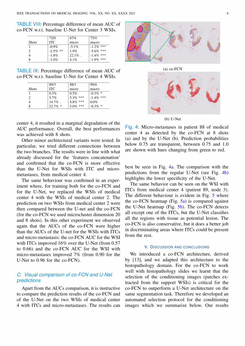
Apart from the AUCs comparison, it is instructiveto compare the prediction results of the co-FCN andof the U-Net on the two WSIs of medical center4 with ITCs and micro-metastases. The results can

(a) co-FCN

(b) U-Net

Fig. 4: Micro-metastases in patient 88 of medicalcenter 4 as detected by the co-FCN at 8 shots(a) and by the U-Net (b). Prediction probabilitiesbelow 0.75 are transparent, between 0.75 and 1.0are shown with hues changing from green to red.

best be seen in Fig. 4a. The comparison with thepredictions from the regular U-Net (see Fig. 4b)highlights the lower specificity of the U-Net.

The same behavior can be seen on the WSI withITCs from medical center 4 (patient 89, node 3).The different behaviour is evident in Fig. 5 wherethe co-FCN heatmap (Fig. 5a) is compared againstthe U-Net heatmap (Fig. 5b). The co-FCN detectsall except one of the ITCs, but the U-Net classifiesall the regions with tissue as potential lesion. Theco-FCN is also conservative, but it does a better jobin discriminating areas where ITCs could be presentfrom the rest.

V. DISCUSSION AND CONCLUSIONS

We introduced a co-FCN architecture, derivedby [13], and we adapted this architecture to thehistopathology domain. For the co-FCN to workwell with histopathology slides we learnt that theselection of the conditioning images (patches ex-tracted from the support WSIs) is critical for theco-FCN to outperform a U-Net architecture on thesame segmentation task. Therefore we developed anautomated selection protocol for the conditioningimages which we summarize below. Our results

IEEE TRANSACTIONS ON MEDICAL IMAGING, VOL. XX, NO. XX, XXXX 2021 9

(a) co-FCN

(b) U-Net

Fig. 5: ITCs in patient 89 of medical center 4 asdetected by the co-FCN at 8 shots (a) and by theU-Net (b). Prediction probabilities below 0.75 aretransparent, the others are shown with hues fromgreen (0.75) to red (1.0).

show that the co-FCN achieves better performanceover a similarly trained U-Net, in that it predictslesion regions on WSIs, containing ITCs and micro-metastases, collected with a digital scanner and froma medical center not used for the collection of thetraining WSIs.

A. Domain adaptation

In reference to WSIs from medical center 4,which uses a digital slide scanner not used inany other centers, the benchmark U-Net containsmore false positives than the co-FCN trained onthe same set of WSIs but conditioned on a supportset from center 4. This is true in particular for themore difficult WSIs containing ITCs and micro-metastases:

• the best AUC for the WSI of patient 89 (con-taining ITCs) obtained by the U-Net is 0.589±0.070, a result which is outperformed by 20%with a co-FCN at 8 shots: 0.708± 0.091;

• the best AUC for the WSI of patient 88 (con-taining micro-metastases) obtained by the U-Net 0.943± 0.008 is slightly improved by 5%with a co-FCN at 8 shots: 0.990± 0.006

The difference in the latter case, due to the highnumber of false positives raised by the U-Net, ismore evident when applying the pAUC metric5 inthe specificity range 90%-100%. In this case the U-Net tops at 0.720 pAUC a result improved by 34.4%by the co-FCN, which achieves a pAUC of 0.968.

The co-FCN therefore performs better than astandard U-Net when facing domain shift and couldbe used, without retraining, to screen WSIs for thepossible presence of ITCs and micro-metastases.

B. Advantages of our support set selectionmethod

Finally, we note that an advantage of our supportselection method is that, to compute the lesionprobability estimate πl for each cluster (see Sub-section III-C.2), only patch-level classification isrequired, instead of a full dense annotation of theexample WSIs from where the patches are extracted.This allows for the usage of sparse annotations tocreate the reference set for selecting support shots,with a net reduction in the annotation effort bypathologists. This is in keeping with the findingsby Rakelly et al. [12] in their architecture who alsoused sparse annotations in their support set.

Future work will explore the interaction betweenthe latent representation extracted by the Condition-ing Branch and the Segmenter output. Furthermore,as the selection of the support set is a crucial step forthe successful training and inference of the co-FCN,we believe that the study of unsupervised strategiesand methods for the proper selection of the supportset remains a promising research topic.

REFERENCES

[1] A. C. Voogd, et al., “Differences in risk factors for local and dis-tant recurrence after breast-conserving therapy or mastectomyfor stage I and II breast cancer: Pooled results of two largeEuropean randomized trials,” Journal of Clinical Oncology,vol. 19, no. 6, pp. 1688–1697, 2001.

[2] P. A. Cronin and M. L. Gemignani, “Breast diseases,”in Clinical Gynecologic Oncology (Ninth Edition), 9thed., Philadelphia, PA, USA: Elsevier, 2018, pp. 320–352.e6. [Online]. Available: https://www.sciencedirect.com/science/article/pii/B9780323400671000140

5The partial AUC (pAUC) is a measure of the AUC of the ROCcurve over a range of interest, either a specificity or sensitivity range[26].

IEEE TRANSACTIONS ON MEDICAL IMAGING, VOL. XX, NO. XX, XXXX 2021 10

[3] G. Litjens et al., “Deep learning as a tool for increased ac-curacy and efficiency of histopathological diagnosis,” ScientificReports, 2016.

[4] N. Dimitriou, O. Arandjelovic, and P. D. Caie, “Deep Learningfor Whole Slide Image Analysis: An Overview,” Frontiers inMedicine, vol. 6, nov 2019.

[5] D. Wang et al., “Mixed-Supervised Dual-Network forMedical Image Segmentation,” Lecture Notes in ComputerScience (including subseries Lecture Notes in ArtificialIntelligence and Lecture Notes in Bioinformatics), vol.11765 LNCS, pp. 192–200, jul 2019. [Online]. Available:http://arxiv.org/abs/1907.10209

[6] C. L. Srinidhi, O. Ciga, and A. L. Martel, “Deepneural network models for computational histopathology:A survey,” Medical Image Analysis, vol. 67, jan 2021.[Online]. Available: https://www.sciencedirect.com/science/article/pii/S1361841520301778

[7] K. Stacke, G. Eilertsen, J. Unger, and C. Lundstrom, “A CloserLook at Domain Shift for Deep Learning in Histopathology,”sep 2019. [Online]. Available: http://arxiv.org/abs/1909.11575

[8] D. Komura and S. Ishikawa, “Machine Learning Methods forHistopathological Image Analysis,” Computational and Struc-tural Biotechnology Journal, vol. 16, pp. 34–42, 2018.

[9] M. Raghu, C. Zhang, J. Kleinberg, and S. Bengio, “Transfusion:Understanding Transfer Learning for Medical Imaging,” feb2019. [Online]. Available: http://arxiv.org/abs/1902.07208

[10] J. Ren, I. Hacihaliloglu, E. A. Singer, D. J. Foran, andX. Qi, “Unsupervised Domain Adaptation for Classification ofHistopathology Whole-Slide Images,” Frontiers in Bioengineer-ing and Biotechnology, vol. 7, may 2019.

[11] O. Ronneberger, P. Fischer, and T. Brox, “U-Net: ConvolutionalNetworks for Biomedical Image Segmentation.” Springer,Cham, 2015, pp. 234–241. [Online]. Available: https://link.springer.com/chapter/10.1007%2F978-3-319-24574-4 28

[12] K. Rakelly, E. Shelhamer, T. Darrell, A. A. Efros, and S. Levine,“Few-Shot Segmentation Propagation with Guided Networks,”may 2018. [Online]. Available: http://arxiv.org/abs/1806.07373

[13] A. Guha Roy, S. Siddiqui, S. Polsterl, N. Navab, andC. Wachinger, “‘Squeeze & excite’ guided few-shot segmen-tation of volumetric images,” Medical Image Analysis, vol. 59,p. 101587, jan 2020.

[14] A. Medela et al., “Few shot learning in histopathological im-ages: Reducing the need of labeled data on biological datasets,”in Proceedings - International Symposium on Biomedical Imag-ing, vol. 2019-April. IEEE Computer Society, apr 2019, pp.1860–1864.

[15] E. van der Spoel et al., “Siamese Neural Networks for One-Shot Image Recognition,” ICML - Deep Learning Workshop,vol. 7, no. 11, pp. 956–963, 2015.

[16] A. Zhao, G. Balakrishnan, F. Durand, J. V. Guttag, and A. V.Dalca, “Data augmentation using learned transformations forone-shot medical image segmentation,” in Proceedings of theIEEE Computer Society Conference on Computer Vision andPattern Recognition, vol. 2019-June, 2019, pp. 8535–8545.

[17] A. R. Feyjie, R. Azad, M. Pedersoli, C. Kauffman, I. B.Ayed, and J. Dolz, “Semi-supervised few-shot learning formedical image segmentation,” 2020. [Online]. Available:http://arxiv.org/abs/2003.08462

[18] G. Litjens et al., “1399 H&E-stained sentinel lymphnode sections of breast cancer patients: The CAMELYONdataset,” pp. 1–8, jun 2018. [Online]. Available: https://www.ncbi.nlm.nih.gov/pmc/articles/PMC6007545

[19] J. Snell, K. Swersky, and R. Zemel, “PrototypicalNetworks for Few-shot Learning,” in Advances inNeural Information Processing Systems, vol. 30.,Curran Associates, Inc., 2017, pp. 4077–4087. [On-line]. Available: https://proceedings.neurips.cc/paper/2017/file/cb8da6767461f2812ae4290eac7cbc42-Paper.pdf

[20] L. Jing and Y. Tian, “Self-supervised visual feature learningwith deep neural networks: A survey,” feb 2019. [Online].Available: http://arxiv.org/abs/1902.06162

[21] A. Paszke et al., “PyTorch: An imperative style, high-performance deep learning library,” in Advances in NeuralInformation Processing Systems, 2019.

[22] W. Falcon, “Pytorch lightning,” GitHub. Note:https://github.com/PyTorchLightning/pytorch-lightning, vol. 3,2019.

[23] X. Robin et al., “pROC: An open-source package for R and S+to analyze and compare ROC curves,” BMC Bioinformatics,2011.

[24] E. R. DeLong, D. M. DeLong, and D. L. Clarke-Pearson,“Comparing the Areas under Two or More Correlated ReceiverOperating Characteristic Curves: A Nonparametric Approach,”Biometrics, 1988.

[25] X. Sun and W. Xu, “Fast implementation of delong’s algorithmfor comparing the areas under correlated receiver operatingcharacteristic curves,” IEEE Signal Processing Letters, vol. 21,no. 11, pp. 1389–1393, 2014.

[26] S. D. Walter, “The partial area under the summary roc curve,”Statistics in Medicine, vol. 24, no. 13, pp. 2025–2040, 2005.[Online]. Available: https://onlinelibrary.wiley.com/doi/abs/10.1002/sim.2103