This report is submitted in partial fulfillment of the requirements for the degree of Bachelor of Computing and Mathematical Sciences with Honours (BCMS(Hons))

at The University of Waikato.

COMP520-14C (HAM)

© 2014 Henry G.R. Gouk

Accelerating Convolutional

Neural Network Systems

Henry G.R. Gouk

Abstract

Convolutional Neural Networks have recently been shown to be highly effec-

tive classifiers for image and speech data. Due to the large volume of data

required to build useful models, and the complexity of the models them-

selves, efficiency has become one of the primary concerns. This work shows

that frequency domain methods can be utilised to accelerate the performance

training, inference, and sliding window classification, despite the problem of

CNNs using small kernels. A speedup is demonstrated on several applications

including traffic sign detection and a range image classification tasks.

Acknowledgements

First and foremost, I would like to thank supervisor, Anthony Blake, for the

inspiration and guidance he has given me. I would also like to thank John

Perrone for the discusions about biologically accurate neural networks, and

both Michael Cree and John for the feedback they provided.

I am greatful to the other members of the Advanced Computation Group for

the interesting discussions and wish them well for their respective projects.

I would also like to thank Joanna for helping me gather New Zealand traffic

sign images, that I was unfortunately not able to utilise due to time con-

straints.

Finally, thanks go to all my other friends and family for tolerating my inces-

sant rambling about what I have been doing all year.

Contents

1 Introduction 1

1.1 Motivation . . . . . . . . . . . . . . . . . . . . . . . . . . . . . 2

1.2 Scope . . . . . . . . . . . . . . . . . . . . . . . . . . . . . . . 3

2 Background 4

2.1 Convolutional Neural Networks . . . . . . . . . . . . . . . . . 4

2.2 Previous Work . . . . . . . . . . . . . . . . . . . . . . . . . . 5

3 Accelerating Training 8

3.1 Frequency Domain Methods . . . . . . . . . . . . . . . . . . . 9

3.1.1 Forward Propagation . . . . . . . . . . . . . . . . . . . 10

3.1.2 Backpropagation . . . . . . . . . . . . . . . . . . . . . 12

3.2 Signals of Arbitrary Dimensions . . . . . . . . . . . . . . . . . 15

3.2.1 Fourier Transforms . . . . . . . . . . . . . . . . . . . . 15

3.2.2 Padded Signal Reversal . . . . . . . . . . . . . . . . . . 16

3.2.3 Pooling . . . . . . . . . . . . . . . . . . . . . . . . . . 17

3.3 Implementation Considerations . . . . . . . . . . . . . . . . . 18

3.3.1 Locality Of Reference . . . . . . . . . . . . . . . . . . . 18

3.3.2 SIMD . . . . . . . . . . . . . . . . . . . . . . . . . . . 19

3.3.3 Control Instructions . . . . . . . . . . . . . . . . . . . 20

3.4 Results . . . . . . . . . . . . . . . . . . . . . . . . . . . . . . . 22

4 Accelerating Sliding Window Classification 29

4.1 Method . . . . . . . . . . . . . . . . . . . . . . . . . . . . . . 30

4.1.1 Algorithmic Enhancements . . . . . . . . . . . . . . . . 30

i

4.1.2 Implementation Considerations . . . . . . . . . . . . . 31

4.2 Results . . . . . . . . . . . . . . . . . . . . . . . . . . . . . . . 32

4.3 Memory Consumption . . . . . . . . . . . . . . . . . . . . . . 36

5 Applications 39

5.1 Classification . . . . . . . . . . . . . . . . . . . . . . . . . . . 39

5.1.1 MNIST . . . . . . . . . . . . . . . . . . . . . . . . . . 40

5.1.2 GTSRB . . . . . . . . . . . . . . . . . . . . . . . . . . 41

5.1.3 CIFAR-10 . . . . . . . . . . . . . . . . . . . . . . . . . 42

5.1.4 Extrinsic Performance Evaluation . . . . . . . . . . . . 43

5.2 Object Detection . . . . . . . . . . . . . . . . . . . . . . . . . 44

5.2.1 Results . . . . . . . . . . . . . . . . . . . . . . . . . . . 46

6 Conclusions 48

6.1 Summary . . . . . . . . . . . . . . . . . . . . . . . . . . . . . 48

6.2 Future Work . . . . . . . . . . . . . . . . . . . . . . . . . . . . 49

Appendices 55

A Multi-Dimensional Algorithms 56

B Efficient Complex

Multiplication 59

ii

List of Figures

2.1 A 1-D convolutional network, without a pooling layer. Note

that first and second layers are not fully connected. . . . . . . 5

3.1 Example of a vector operation. Diagram provided by Tim

Leathart. . . . . . . . . . . . . . . . . . . . . . . . . . . . . . . 19

3.2 This pie chart shows the percentage of run time spent exe-

cuting each operation during the training of the CIFAR-10

network described in Chapter 5. . . . . . . . . . . . . . . . . . 21

3.3 A plot of the minibatch size versus the average time per epoch

of training for a convolutional layer with 32 input and output

channels of 64× 64 pixels, with 5× 5 kernels. . . . . . . . . . 23

3.4 A plot of the input dimensions versus the time (seconds) for

training on a convolutional layer. Square input images are

used, with the value of N used for both the width and height. 25

3.5 A plot of the kernel dimensions versus the time (seconds) for

training on a convolutional layer. Square kernels are used,

with the value of N used for both the width and height. . . . 26

3.6 A plot of the relative speedup of the frequency domain ap-

proach over the spatial domain approach as the number of

input channels is varied. . . . . . . . . . . . . . . . . . . . . . 27

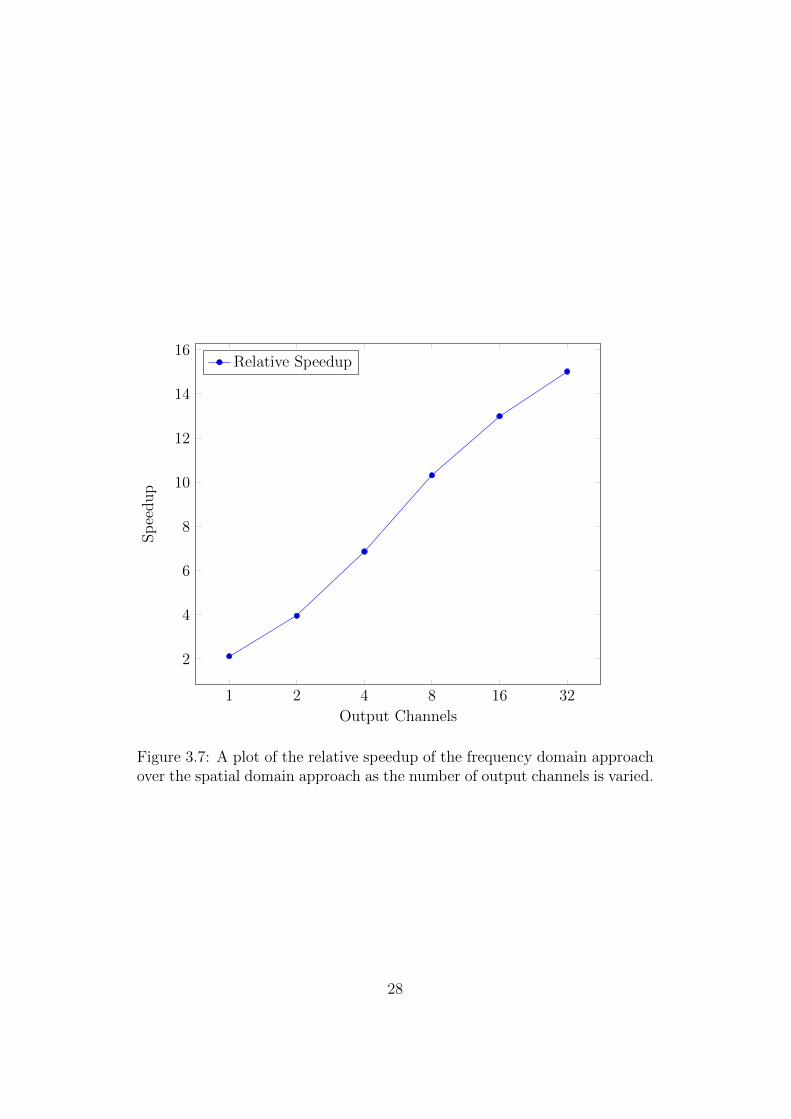
3.7 A plot of the relative speedup of the frequency domain ap-

proach over the spatial domain approach as the number of

output channels is varied. . . . . . . . . . . . . . . . . . . . . 28

iii

4.1 A plot of the input dimensions versus the time (seconds) for

sliding inference with a convolutional layer. Square input im-

ages are used, with the value of N used for both the width and

height. The kernels were 5× 5 pixels, and there were 32 input

and output channels. A sub-window size of 32 × 32 pixels is

used. . . . . . . . . . . . . . . . . . . . . . . . . . . . . . . . . 34

4.2 A plot of the sub-window dimensions versus the time (seconds)

for sliding inference with a convolutional layer. 512×512 pixel

input images are used, the kernels were 5×5 pixels, and there

were 32 input and output channels. . . . . . . . . . . . . . . . 35

4.3 A plot of the relative speedup of the unrolled sliding window

fully connected layer over using a space domain convolutional

layer with 1× 1 kernels. . . . . . . . . . . . . . . . . . . . . . 37

5.1 A collection of images from the MNIST dataset. . . . . . . . . 41

5.2 A collection of images from the GTSRB dataset. . . . . . . . . 42

5.3 A collection of images from the CIFAR-10 dataset. Source:

http://www.cs.toronto.edu/~kriz/cifar.html . . . . . . . 43

5.4 A plot showing the average time over 10 runs required to train

on 10,000 images from the MNIST, GTSRB, and CIFAR-10

datasets for the four different CNN implementations. . . . . . 45

5.5 This figure shows how each of the algorithms performs as the

dimensions of the image given to the network grows. . . . . . . 47

iv

List of Algorithms

1 Computes the activations of a convolutional layer using the

space domain convolution algorithm. . . . . . . . . . . . . . . 10

2 Computes the activations of a convolutional layer using the

frequency domain convolution algorithm. . . . . . . . . . . . . 11

3 Computes the derivative of the cost function with respect to

each activation in the layer previous to a convolutional layer

using space domain methods. . . . . . . . . . . . . . . . . . . 12

4 Computes the derivative of the cost function with respect to

each activation in the layer previous to a convolutional layer

using frequency domain methods. . . . . . . . . . . . . . . . . 13

5 Computes the error derivatives with respect to each weight in

a convolutional layer, with the cross correlation performed in

the space domain. . . . . . . . . . . . . . . . . . . . . . . . . . 14

6 Computes the error derivatives with respect to each weight in

a convolutional layer, with the cross correlation performed in

the frequency domain. . . . . . . . . . . . . . . . . . . . . . . 15

7 Reverses the R dimensional signal I of size D and zero pads

it to be of size P . Zeros returns a signal of the specified

dimensions where every data point is a zero. . . . . . . . . . . 16

8 Finds the maximal element in each non-overlapping section of

a uniformly subdivided hypercube. . . . . . . . . . . . . . . . 17

9 Pads the rank R input tensor, I, of size D to be of size P . . . 57

v

10 Crops the rank R input tensor, I, from size D to size V , taking

into account a translation in each dimension introduced by the

frequency domain convolution algorithm. . . . . . . . . . . . . 57

11 Crops the rank R input tensor, I, from size D to size V , taking

into account a translation in each dimension introduced by the

frequency domain convolution algorithm. The output is also

reversed in each dimension. . . . . . . . . . . . . . . . . . . . 58

12 Crops the rank R input tensor, I, from size D to size V and

reverses the result in each dimension. . . . . . . . . . . . . . . 58

vi

Chapter 1

Introduction

“The question of whether a computer can think is no more interesting than

the question of whether a submarine can swim.”

— Edsger Dijkstra

For decades Machine Learning and Computer Vision researchers have at-

tempted to construct computer systems capable of understanding their sur-

roundings as seen through the lens of a camera. Whether this understanding

comes in the form of being able to discriminate between different objects or

the ability to manipulate actuators to interact with the environment, progress

has been slow but steady. Many attempts were built around hand crafted

rules or basic statistical analysis, but people inevitably looked to the brain as

an example of how this goal could be accomplished by a proven system. The

result of this was the introduction of many algorithms, collectively dubbed

“neural networks”, accompanied by claims that they mimic how a human

visual cortex interprets the world.

While it is far-fetched to state that these algorithms are biologically accurate,

it cannot be denied that some are at least biologically inspired. Convolutional

1

Neural Networks (CNN) are one of the best examples of this. The convolu-

tional and pooling layers were directly inspired by the results of Hubel and

Wiesel’s experiments that revealed the presence of simple and complex cells

in the visual cortex [1]. The usage of these two types of layers is the main

factor in the success of CNNs over other machine learning algorithms when

performing pattern recognition tasks on natural signals – particularly image

classification. Although CNNs were first developed almost 25 years ago, it is

only recently that they have started to outperform other methods in popu-

lar object recognition benchmarks. This is often attributed the ever-growing

image datasets and the greatly increased computing power available today,

allowing larger and more sophisticated models to be built.

1.1 Motivation

Despite this increase in the performance of modern computing systems, train-

ing a modestly sized CNN model is still time consuming. Compounded with

the fact that neural networks have a large number of model hyperparameters

that must be assigned sensible values through a trial and error process –

such as a grid search or Bayesian hyperparameter optimisation – this causes

the total time required to build an accurate model to increase massively. As

such, the first goal of this project is to design a system that can train CNNs

much faster than the conventional methods.

In addition to networks taking a long time to train, there is also the problem

of efficiently using a deployed CNN system. This is still quite a broad problem

in itself, as the context of how inference is performed using the CNN is quite

important. For example, if one is simply classifying a set of fixed sized

images then the standard inference procedure, or some optimised variant,

can be used. However, if the CNN is part of a larger system, then it is likely

that the global structure of the system can be optimised in some way to

maximise performance.

This project aims to improve the efficiency of training CNNs, and also the

2

methods used for inference in a variety of applications. Advances in these

areas have the potential to greatly reduce operating costs of large computer

systems that rely heavily on CNNs to make predictions, as well as enabling

new applications that were previously unfeasible.

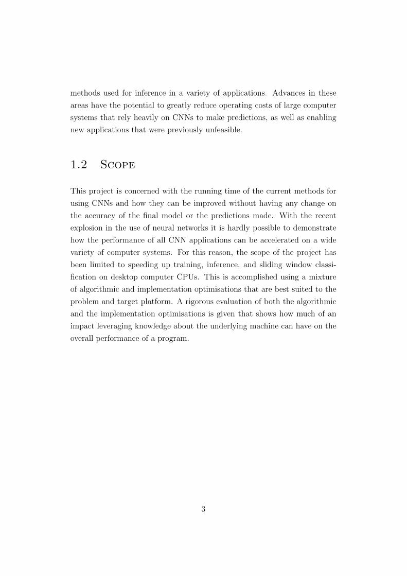
1.2 Scope

This project is concerned with the running time of the current methods for

using CNNs and how they can be improved without having any change on

the accuracy of the final model or the predictions made. With the recent

explosion in the use of neural networks it is hardly possible to demonstrate

how the performance of all CNN applications can be accelerated on a wide

variety of computer systems. For this reason, the scope of the project has

been limited to speeding up training, inference, and sliding window classi-

fication on desktop computer CPUs. This is accomplished using a mixture

of algorithmic and implementation optimisations that are best suited to the

problem and target platform. A rigorous evaluation of both the algorithmic

and the implementation optimisations is given that shows how much of an

impact leveraging knowledge about the underlying machine can have on the

overall performance of a program.

3

Chapter 2

Background

“Geoff Hinton discovered how the brain really works. Once a year for the

last 25 years.”

— Yann LeCun

This chapter describes the current trends in neural network research and

where the work conducted during this project fits in with key developments

in the field. Firstly, the differences between MLPs and CNNs are presented,

and then a short review of previous milestones in specific areas relevant to

this project are given.

2.1 Convolutional Neural Networks

CNNs can be viewed as extensions to MLPs in two different ways. In one view

the convolutional and pooling layers are introduced as completely new types

of layers tasked with learning a feature representation that is then fed into a

normal MLP. What makes convolutional layers different from fully connected

layers is the local connectivity and the shared weights. That is, each unit in a

4

Figure 2.1: A 1-D convolutional network, without a pooling layer. Note thatfirst and second layers are not fully connected.

convolutional layer takes only a subset of the activations in the previous layer

as input, and groups of units in convolutional layers share the same weight

vector. Pooling layers are then used as a way to accumulate local groups of

activations produced by the convolutional layers. Figure 2.1 demonstrates

how these layers are connected in the case where a one dimensional signal is

being classified.

In the other view, convolutional layers are considered to be an abstraction of

fully connected layers that operate on tensors instead of scalars, with convo-

lution used in place of multiplication and pointwise addition used instead of

regular addition. The input feature maps, output feature maps, and kernels

can all be considered tensors and the pooling layers can be thought of as

extensions to the activation functions.

2.2 Previous Work

It has been shown both theoretically and empirically that the number of

hidden units in a CNN is strongly correlated to its predictive power [2, 3].

This alone is a compelling reason to accelerate both the rate at which CNNs

5

can be trained and the speed at which inferences can be performed on newly

supplied data. Coupled with this is the desire to scale CNN models to much

harder problems with more classes and more complex images [4]. In addition,

problems such as object detection and reinforcement learning systems often

have real-time constraints.

A plethora of research has been conducted with the aim of shortening the

length of time required for CNNs and, more broadly, ANNs to converge

towards states of minimal error. The methods produced by this work can be

approximately separated into two categories: those that reduce the number

of times each instance is processed, and those that reduce the average length

of time taken to process each instance.

The first category is comprised of methods like Stochastic Gradient Descent

(SGD), the Conjugate Gradient method, and L-BFGS — see [5] for a per-

formance comparison in the context of CNNs. This category also includes

augmentations to these training algorithms, such as momentum, Nesterov’s

accelerated gradient [6], weight initialization heuristics [7, 8], and various

adaptive learning rate schemes [9, 10, 11]. All of these algorithms belong to

the field of numerical optimisation, and can be applied to many problems

other than training neural networks.

The second category is mainly composed of methods that utilise aspects in-

herent to the target platform of the CNN implementation. For example, GPU

implementations have become more popular than CPU implementations due

to the ability of processors belonging to the GPU architecture paradigm

to run a simple program in an embarrassingly parallel manner [4, 12, 13].

Extending the idea of massively parallel computations, some cluster based

implementations are starting to emerge. Google recently received media cov-

erage for their cluster based neural network implementation that used an

asynchronous numerical optimisation algorithm to exploit parallelism be-

tween many high speed processors [3]. FPGA implementations have also

started to be explored, with the primary focus being on high speed infer-

ence [14, 15], allowing efficient deployment for embedded applications.

6

The work undertaken during this project pertaining to the acceleration of

CNNs is based off research conducted during a directed study by the author

in the previous year [16]. During the course of this study the forward prop-

agation procedure and part of the training procedure was transformed to be

carried in the frequency domain by exploiting the convolution theorem and

the linearity property of the Fourier transform. This resulted in a substantial

improvement in performance, due to a time complexity change allowing the

procedures to scale better to larger networks and input signals. Since that

study was conducted another group has implemented a similar system that

uses frequency domain methods to train networks [17]. This project extends

the ideas presented during the directed study to achieve further accelera-

tion of the training procedure, and also greatly increases the performance of

applying CNNs as sliding window classifiers.

7

Chapter 3

Accelerating Training

“With four parameters I can fit an elephant, and with five I can make him

wiggle his trunk.”

— John von Neumann

Recently the image datasets available for training CNNs have rapidly grown

in size, with respect to the number of images and the size of each image [18].

The first goal of this project was to design a system that allows for training

on large datasets in a more scaleable manner.

When faced with the problem of optimising the performance of a system,

one must carefully scrutinise the system at every level of abstraction in order

to devise a solution that will provide a high level of performance. In the

context of training CNNs this involved looking at the entire system that

encompasses the CNN, the algorithms used, their implementations, and the

hardware executing the machine code. In other words, optimisations were

performed at several layers of abstraction.

8

3.1 Frequency Domain Methods

The idea of using frequency domain methods to accelerate the training of

CNNs was first introduced during a directed study carried out during the year

previous to this project [16], and also explored by [17]. Over the course of this

study algorithms that exploit frequency domain characteristics of signals were

devised to speed up the forward propagation and backpropagation procedures

involved in the training process. In the report it is mentioned that further

improvements could be made by transforming more of the training process to

use frequency domain methods. The process of achieving this enhancement is

described in this section. A concise derivation of the entire frequency domain

set of methods is given, including those developed during the directed study.

The training process can be divided into four distinct phases:

Forward Propagation is the process of performing an inference on the sup-

plied instance. The current predictions made by the CNN are required

in order to compute the error attributable to each instance, which is

needed to modify the weights of the network.

Backpropagation is the procedure used to compute the derivative of the

error function with respect to each weight in the network. In this work

backpropagation refers to calculating the error derivative with respect

to the activation value of each unit in the network.

Gradient Calculation is actually the second part of the backpropagation

procedure. During this phase the error derivatives with respect to the

activations are used to calculate the derivatives for each weight.

Weight Updating is done after the error derivatives with respect to each

weight have been accumulated for a minibatch. These gradients are

then used to change the weights in such a way that the error is likely

to be reduced. In this work SGD is used as the update rule.

The forward propagation, gradient calculation, and weight update stages

were all modified to use frequency domain methods in [16], leaving just the

9

Algorithm 1 Computes the activations of a convolutional layer using thespace domain convolution algorithm.

function SpaceForward(I, N , M , K, B, g)for o = 1 to M do

for i = 1 to N doOo ← Oo + Ii ∗Ko,i

end forOo ← g(Oo + Bo)

end forreturn O

end function

remainder of the backpropagation procedure to be changed in this work and

new performance measurements to be carried out.

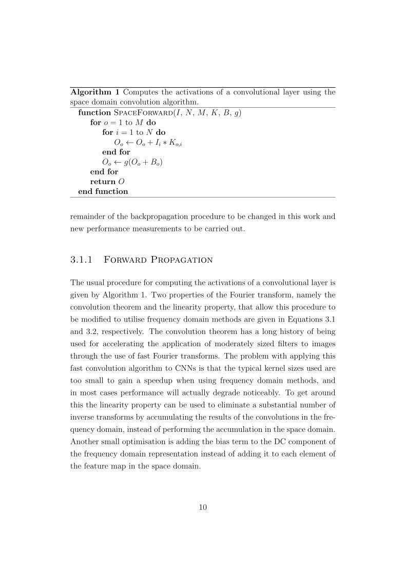
3.1.1 Forward Propagation

The usual procedure for computing the activations of a convolutional layer is

given by Algorithm 1. Two properties of the Fourier transform, namely the

convolution theorem and the linearity property, that allow this procedure to

be modified to utilise frequency domain methods are given in Equations 3.1

and 3.2, respectively. The convolution theorem has a long history of being

used for accelerating the application of moderately sized filters to images

through the use of fast Fourier transforms. The problem with applying this

fast convolution algorithm to CNNs is that the typical kernel sizes used are

too small to gain a speedup when using frequency domain methods, and

in most cases performance will actually degrade noticeably. To get around

this the linearity property can be used to eliminate a substantial number of

inverse transforms by accumulating the results of the convolutions in the fre-

quency domain, instead of performing the accumulation in the space domain.

Another small optimisation is adding the bias term to the DC component of

the frequency domain representation instead of adding it to each element of

the feature map in the space domain.

10

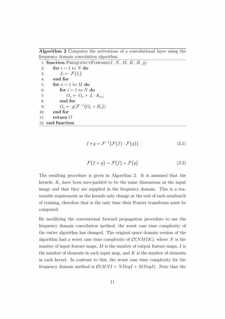
Algorithm 2 Computes the activations of a convolutional layer using thefrequency domain convolution algorithm.

1: function FrequencyFoward(I, N , M , K, B, g)2: for i = 1 to N do3: Ji ← F{Ii}4: end for5: for o = 1 to M do6: for i = 1 to N do7: Oo ← Oo + Ji ·Ko,i

8: end for9: Oo ← g(F−1{Oo + Bo})

10: end for11: return O12: end function

f ∗ g = F−1{F{f} · F{g}} (3.1)

F{f + g} = F{f}+ F{g} (3.2)

The resulting procedure is given in Algorithm 2. It is assumed that the

kernels, K, have been zero-padded to be the same dimensions as the input

image and that they are supplied in the frequency domain. This is a rea-

sonable requirement as the kernels only change at the end of each minibatch

of training, therefore that is the only time their Fourier transforms must be

computed.

By modifying the conventional forward propagation procedure to use the

frequency domain convolution method, the worst case time complexity of

the entire algorithm has changed. The original space domain version of the

algorithm had a worst case time complexity of O(NMIK), where N is the

number of input feature maps, M is the number of output feature maps, I is

the number of elements in each input map, and K is the number of elements

in each kernel. In contrast to this, the worst case time complexity for the

frequency domain method is O(MNI + NIlogI + MIlogI). Note that the

11

Algorithm 3 Computes the derivative of the cost function with respect toeach activation in the layer previous to a convolutional layer using spacedomain methods.1: function SpaceBackward( δJ

δz, K, N , M)

2: for i = 1 to N do3: for o = 1 to M do4: Bi ← Bi + δJ

δzo∗Reverse(Ko,i)

5: end for6: end for7: return B8: end function

running time of the algorithm no longer depends on the size of the kernels

used.

3.1.2 Backpropagation

The backpropagation procedure is responsible for computing the derivative

of the cost function, J(~x), with respect to each weight in the network. These

values are then accumulated across a set of the training instances and used

to perform a weight update. This process can be further divided into two

parts; computing δJδw

, where w is a weight, and computing δJδa

, where a is the

activation of a unit in the previous layer.

The first stage of the backpropagation procedure is responsible for actually

backpropagating the errors of one layer to the preceding layer in the network.

The space domain algorithm for calculating the derivative of the cost with

respect to each unit in the previous layer of the network is given in Algo-

rithm 3. In the two dimensional case, reversing the kernel in each dimension

has the same effect as rotating it by 180 degrees. By convolving the error

derivatives, δJδa

, with the rotated kernel, the cross-correlation between the two

signals is computed.

The strategy used to accelerate the forward propagation can also be applied

here. One potential problem with directly applying the same technique is

that kernels must be rotated and padded before the convolution operation

12

Algorithm 4 Computes the derivative of the cost function with respect toeach activation in the layer previous to a convolutional layer using frequencydomain methods.1: function FrequencyBackward( δJ

δz, K, N , M)

2: for i = 1 to N do3: for o = 1 to M do4: Bi ← Bi + δJ

δzo·Ko,i

5: end for6: Bi ← F−1{CropReverse(Bi)}7: end for8: return B9: end function

is performed. Since the kernels have been supplied in the frequency domain

this would require transforming them back into the space domain, padding

and rotating the image, and then once again transforming them into the fre-

quency domain. Alternatively, one could take the complex conjugate of each

kernel to perform the reversal, and then modify the imaginary component

of each element to affect a translation equivalent to padding. This option is

computation heavy compared to the third option; reverse each error deriva-

tive map for this layer (which is already done during the calculate gradients

step), and then reverse the result of the cross correlation, yielding an error

derivative map for the previous layer in the network. Algorithm 4 provides

pseudocode for this method. Once again the kernels are expected to be in

the frequency domain, but in this case derivatives, δJδz

, are also expected to

be in the frequency domain. This can be accomplished by simply storing

these values when they are computed during the gradient calculation step.

As with the forward propagation procedure, the worst case time complexity of

the space domain method for backpropagation is O(NMIK), and O(NMI+

NIlogI) for the frequency domain method.

The gradient calculation stage of the backpropagation procedure uses the er-

ror derivatives with respect to each unit in a convolutional layer to compute

the error derivatives with respect to each weight in the layer. The conven-

tional approach to performing the step is outlined in Algorithm 5. Note that

13

Algorithm 5 Computes the error derivatives with respect to each weightin a convolutional layer, with the cross correlation performed in the spacedomain.1: function SpaceCalculateGradients( δJ

δK, δJδa

, δaδz

, I, N , M)2: for o = 1 to M do3: δJ

δzo← δJ

δao· δaδzo

4: δJδbo←SumComponents( δJ

δzo)

5: for i = 1 to N do6: T ← Ii∗Reverse( δJ

δzo)

7: δJδKo,i

← δJδKo,i

+Reverse(T )

8: end for9: end for

10: return ( δJδK

, δJδb

)11: end function

the second call to reverse that takes the result of the cross correlation as a

parameter is actually deferred until the end of each minibatch, where it is

applied to the derivatives accumulated over the entire minibatch.

By applying optimisations similar to those used in the forward propaga-

tion and backpropagation procedures one can derive a faster algorithm for

computing these derivatives. The cross correlation can be performed in the

frequency domain, and because the input features to each convolutional layer

have already been transformed into the frequency domain during the forward

propagation stage there is no need to recompute this data. The linearity

property can once again be exploited, allowing the values to be accumulated

in the frequency domain instead of transforming the data back into the space

domain. These inverse transforms can be delayed until the end of the mini-

batch. The resulting algorithm is given in Algorithm 6, and has a worst case

time complexity of O(NMI + MIlogI), as opposed to O(NMIK) for the

space domain approach.

14

Algorithm 6 Computes the error derivatives with respect to each weight ina convolutional layer, with the cross correlation performed in the frequencydomain.1: function FrequencyCalculateGradients2: for o = 1 to M do3: T ←PadReverse( δJ

δao· δaδzo

)

4: δJδbo←SumComponents(T )

5: δJδzo← F{T}

6: for i = 1 to N do7: S ← Ji · δJδzo8: δJ

δKo,i← δJ

δKo,i+ S

9: end for10: end for11: end function

3.2 Signals of Arbitrary Dimensions

CNNs have primarily seen use in the domain of image classification, how-

ever audio and video (i.e. 1-D and 3-D) classification systems have also been

built that incorporate CNN models [19, 20]. In order to provide a high speed

implementation of training and inference methods for as many scenarios as

possible, it became necessary to devise algorithms that could perform all the

required operations on data of arbitrary dimensions. In all cases dynamic

programming was used to facilitate multi-dimensional data manipulation.

Quite a few operations are required to implement the procedures in the fre-

quency domain, so only a selection of the dynamic programming algorithms

are described here.

3.2.1 Fourier Transforms

An elegant property of multi-dimensional Fourier transforms is the ability to

express an N dimensional transform as many N − 1 dimensional transforms,

interspersed by transpositions. This happens the be the method most fre-

quently implemented for multi-dimensional transforms in high performance

15

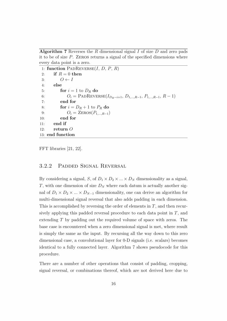
Algorithm 7 Reverses the R dimensional signal I of size D and zero padsit to be of size P . Zeros returns a signal of the specified dimensions whereevery data point is a zero.

1: function PadReverse(I, D, P , R)2: if R = 0 then3: O ← I4: else5: for i = 1 to DR do6: Oi = PadReverse(IDR−i+1, D1,...,R−1, P1,...,R−1, R− 1)7: end for8: for i = DR + 1 to PR do9: Oi = Zeros(P1,...,R−1)

10: end for11: end if12: return O13: end function

FFT libraries [21, 22].

3.2.2 Padded Signal Reversal

By considering a signal, S, of D1×D2× ...×DN dimensionality as a signal,

T , with one dimension of size DN where each datum is actually another sig-

nal of D1 ×D2 × ...×DN−1 dimensionality, one can derive an algorithm for

multi-dimensional signal reversal that also adds padding in each dimension.

This is accomplished by reversing the order of elements in T , and then recur-

sively applying this padded reversal procedure to each data point in T , and

extending T by padding out the required volume of space with zeros. The

base case is encountered when a zero dimensional signal is met, where result

is simply the same as the input. By recursing all the way down to this zero

dimensional case, a convolutional layer for 0-D signals (i.e. scalars) becomes

identical to a fully connected layer. Algorithm 7 shows pseudocode for this

procedure.

There are a number of other operations that consist of padding, cropping,

signal reversal, or combinations thereof, which are not derived here due to

16

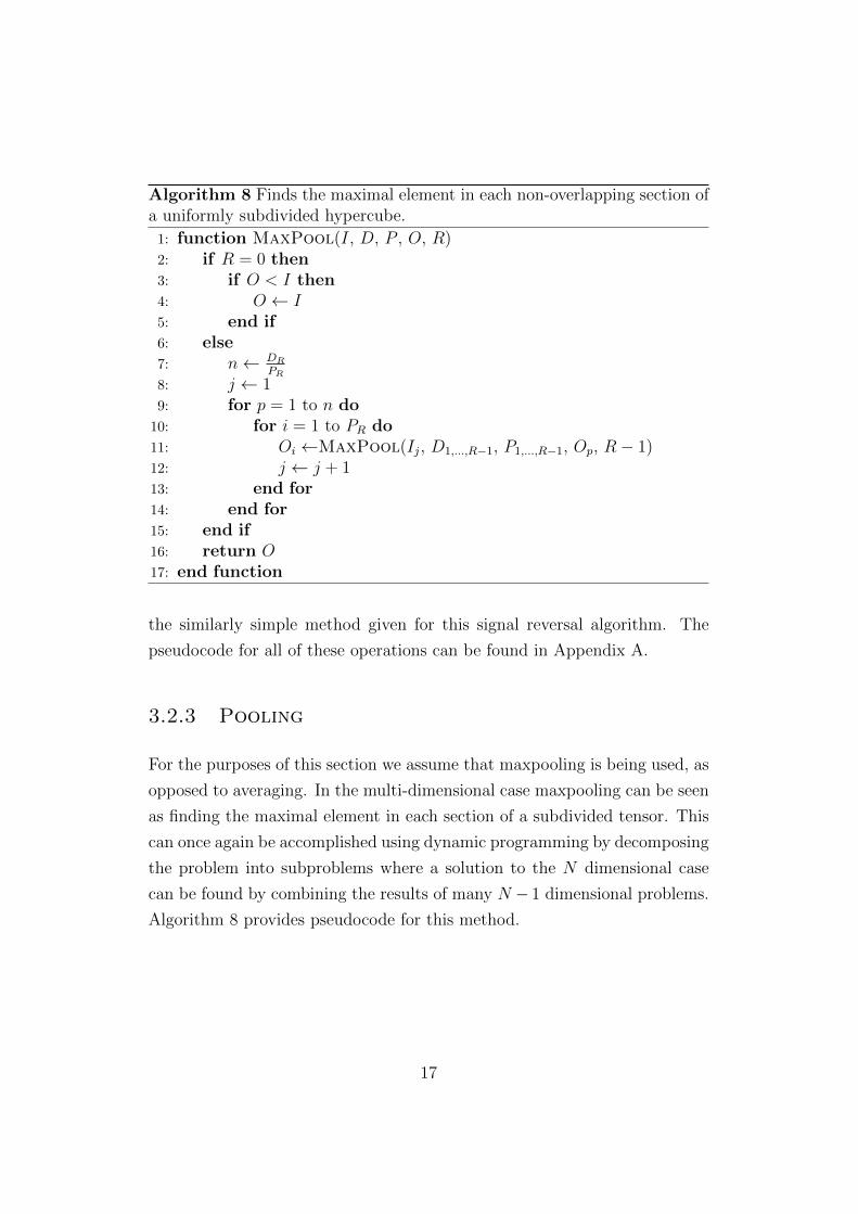
Algorithm 8 Finds the maximal element in each non-overlapping section ofa uniformly subdivided hypercube.

1: function MaxPool(I, D, P , O, R)2: if R = 0 then3: if O < I then4: O ← I5: end if6: else7: n← DR

PR

8: j ← 19: for p = 1 to n do

10: for i = 1 to PR do11: Oi ←MaxPool(Ij, D1,...,R−1, P1,...,R−1, Op, R− 1)12: j ← j + 113: end for14: end for15: end if16: return O17: end function

the similarly simple method given for this signal reversal algorithm. The

pseudocode for all of these operations can be found in Appendix A.

3.2.3 Pooling

For the purposes of this section we assume that maxpooling is being used, as

opposed to averaging. In the multi-dimensional case maxpooling can be seen

as finding the maximal element in each section of a subdivided tensor. This

can once again be accomplished using dynamic programming by decomposing

the problem into subproblems where a solution to the N dimensional case

can be found by combining the results of many N − 1 dimensional problems.

Algorithm 8 provides pseudocode for this method.

17

3.3 Implementation Considerations

The multi-dimensional signal processing algorithms given previously are not

the only way to apply the required operations to signals of arbitrary dimen-

sions. The selection of these algorithms in particular was motivated by how

efficiently they can be implemented on modern computer architectures. Due

to the physical limitations of how small transistors can be constructed, it has

become necessary for microarchitects to introduce new architectural features

that enable programmers to gain increases in performance. The two main

concerns programmers should now have when implementing algorithms effi-

ciently are the memory access patterns, and how well the algorithm can be

vectorised. In this section the techniques used to optimise the C++ imple-

mentation1 of the CNN training and inference procedures are detailed.

3.3.1 Locality Of Reference

To combat the growing disparity between processor and memory perfor-

mance, most modern CPUs contain a cache subsystem tasked with hiding

the latency incurred by accessing the main system memory. As such, it

has become important to analyse how different algorithms will impact cache

behaviour, otherwise an approach that appears to be the asymptotically op-

timal choice could run the risk of having poor performance for the task at

hand due to suboptimal cache utilisation. One of the responsibilities of the

cache subsystem is to determine what should or should not be stored in the

cache. In order to do this, certain assumptions have to be made about how

programs will access memory. The main assumption made by most proces-

sors is the idea that the memory access patterns will exhibit some sort of

locality, whether it be spatial or temporal. That is, CPU caches are designed

to perform well when programs access many nearby memory locations in a

short space of time.

1The implementation has been made open source and is available fromhttp://github.com/henrygouk/nnet

18

5 0 2 4

×3 9 1 4

=

15 0 2 16

Figure 3.1: Example of a vector operation. Diagram provided by TimLeathart.

For the signal processing operations described earlier, the ideal algorithm

would be capable of computing the result in a single linear pass over the

input data. The algorithms given in Section 3.2 and Appendix A have been

designed in such a way that the input signals are accessed as one continuous

stream of data, provided the data is stored in row major order. Because

of this the hardware prefetcher is able to correctly predict which memory

locations will be accessed in future with high accuracy, thus the CPU fetches

data from the main system memory before the program even requests that

data.

3.3.2 SIMD

The frequency at which commodity microprocessors can operate has stag-

nated due to a multitude of physical limitations. To compensate for this

CPU designers have had to innovate at the microarchitecture level, creat-

ing new instructions that allow processors to continue gaining performance

boosts with each generation. The most successful extensions have been the

addition of SIMD (Single Instruction, Multiple Data) instructions that al-

low the same operation to be applied to several data elements at the same

time. This is accomplished by loading data from memory into short vector

registers and then using these SIMD instructions instead of the usual SISD

(Single Instruction, Single Data) instructions. Figure 3.1 gives and example

of a SIMD vector operation.

19

The sequential memory access patterns of the signal processing algorithms

given previously also enables easy vectorisation. This is because the most

efficient instructions to load data into the vector registers require that the

data be stored sequentially in memory. Having the data in organised in a

contiguous manner also simplifies the flow control aspect of the implemen-

tation; the only condition that must be checked on each memory access is

whether there is enough data left to be processed that will fill up a vector

register. In the event that there is not sufficient data to fill a vector register,

scalar instructions must be used otherwise the vector load instruction could

cause a memory safety fault.

As the number of filters in a convolutional layer grows, the pointwise com-

plex multiplication becomes the most performance critical component of the

algorithm. As shown in Figure 3.2, these complex multiplications make up a

substantial fraction of the overall running time. Thus, efficient implementa-

tion of these operations is critical. Due to the sequential nature of pointwise

operations, these complex multiplications were an ideal candidate for vec-

torisation. Appendix B shows how pointwise complex multiplication can

be efficiently implemented using Intels AVX (Advanced Vector eXtensions)

SIMD instructions.

3.3.3 Control Instructions

The superscalar pipelines implemented in modern processors incur a huge

overhead when branch prediction algorithms make mistakes. This, along

with the added overhead of the CPU actually having the execute these control

instructions instead of data instructions, is a strong motivation for reducing

the occurrence of branches as much as possible.

A similar problem, in sense that it also involves control instructions, is the

usage of recursive functions like those given for computing signal processing

operations on multi-dimensional data. Calling functions has the overhead of

setting up a new stack frame, which in turn requires a number of memory

accesses and control instructions. Thus, recursively calling a function inside

20

Operation Breakdown

Pointwise Complex Multiplication

FFT

Maxpool

Pad Image

Other

47.9%

23.6%

7.67%

3.52%17.3%

Figure 3.2: This pie chart shows the percentage of run time spent executingeach operation during the training of the CIFAR-10 network described inChapter 5.

21

nested loops will incur a massive penalty on performance. For the signal pro-

cessing operations this was mitigated by hard coding an iterative algorithm

for the one dimensional cases.

3.4 Results

To quantify how well the frequency domain methods perform versus space

domain methods several experiments were run. These performance mea-

surements demonstrate how the speed of convolutional layers are affected by

varying different network hyperparameters. A comparison between training

times for vectorised and unvectorised implementations of both algorithms

provided with the extrinsic performance evaluation given in Section 5.1.4.

The experiments were all run on a desktop computer with an Intel i7-4770

processor and 16GB of RAM.

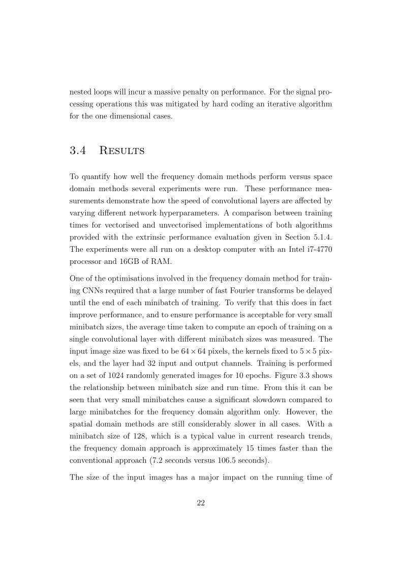
One of the optimisations involved in the frequency domain method for train-

ing CNNs required that a large number of fast Fourier transforms be delayed

until the end of each minibatch of training. To verify that this does in fact

improve performance, and to ensure performance is acceptable for very small

minibatch sizes, the average time taken to compute an epoch of training on a

single convolutional layer with different minibatch sizes was measured. The

input image size was fixed to be 64× 64 pixels, the kernels fixed to 5× 5 pix-

els, and the layer had 32 input and output channels. Training is performed

on a set of 1024 randomly generated images for 10 epochs. Figure 3.3 shows

the relationship between minibatch size and run time. From this it can be

seen that very small minibatches cause a significant slowdown compared to

large minibatches for the frequency domain algorithm only. However, the

spatial domain methods are still considerably slower in all cases. With a

minibatch size of 128, which is a typical value in current research trends,

the frequency domain approach is approximately 15 times faster than the

conventional approach (7.2 seconds versus 106.5 seconds).

The size of the input images has a major impact on the running time of

22

1 2 4 8 16 32 64 1280

20

40

60

80

100

Minibatch Size

Tim

e(s

econ

ds)

Frequency DomainSpace Domain

Figure 3.3: A plot of the minibatch size versus the average time per epochof training for a convolutional layer with 32 input and output channels of64× 64 pixels, with 5× 5 kernels.

23

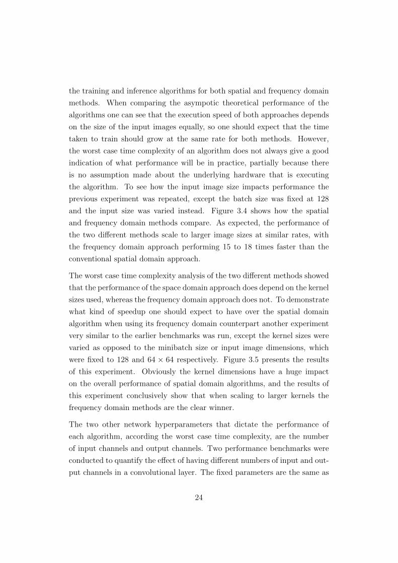
the training and inference algorithms for both spatial and frequency domain

methods. When comparing the asympotic theoretical performance of the

algorithms one can see that the execution speed of both approaches depends

on the size of the input images equally, so one should expect that the time

taken to train should grow at the same rate for both methods. However,

the worst case time complexity of an algorithm does not always give a good

indication of what performance will be in practice, partially because there

is no assumption made about the underlying hardware that is executing

the algorithm. To see how the input image size impacts performance the

previous experiment was repeated, except the batch size was fixed at 128

and the input size was varied instead. Figure 3.4 shows how the spatial

and frequency domain methods compare. As expected, the performance of

the two different methods scale to larger image sizes at similar rates, with

the frequency domain approach performing 15 to 18 times faster than the

conventional spatial domain approach.

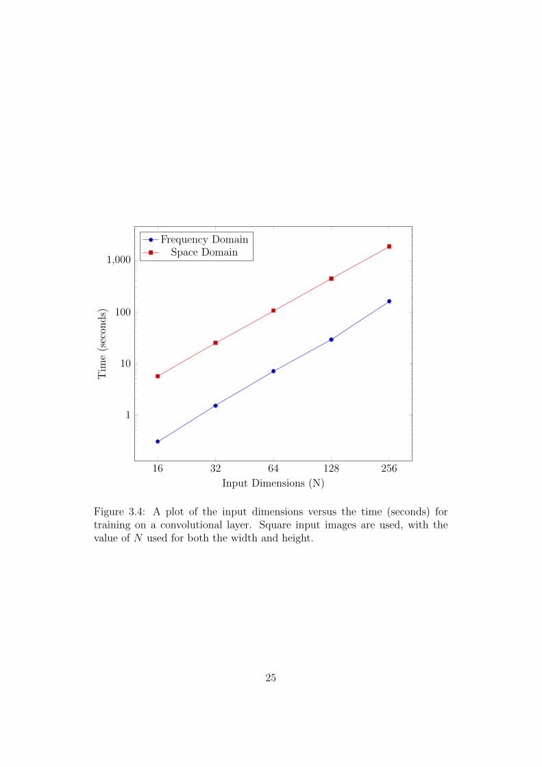
The worst case time complexity analysis of the two different methods showed

that the performance of the space domain approach does depend on the kernel

sizes used, whereas the frequency domain approach does not. To demonstrate

what kind of speedup one should expect to have over the spatial domain

algorithm when using its frequency domain counterpart another experiment

very similar to the earlier benchmarks was run, except the kernel sizes were

varied as opposed to the minibatch size or input image dimensions, which

were fixed to 128 and 64 × 64 respectively. Figure 3.5 presents the results

of this experiment. Obviously the kernel dimensions have a huge impact

on the overall performance of spatial domain algorithms, and the results of

this experiment conclusively show that when scaling to larger kernels the

frequency domain methods are the clear winner.

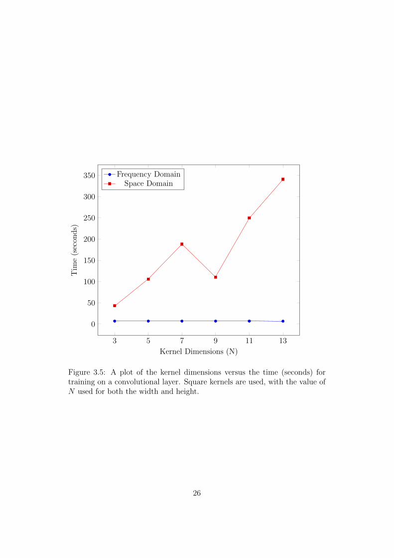
The two other network hyperparameters that dictate the performance of

each algorithm, according the worst case time complexity, are the number

of input channels and output channels. Two performance benchmarks were

conducted to quantify the effect of having different numbers of input and out-

put channels in a convolutional layer. The fixed parameters are the same as

24

16 32 64 128 256

1

10

100

1,000

Input Dimensions (N)

Tim

e(s

econ

ds)

Frequency DomainSpace Domain

Figure 3.4: A plot of the input dimensions versus the time (seconds) fortraining on a convolutional layer. Square input images are used, with thevalue of N used for both the width and height.

25

3 5 7 9 11 13

0

50

100

150

200

250

300

350

Kernel Dimensions (N)

Tim

e(s

econ

ds)

Frequency DomainSpace Domain

Figure 3.5: A plot of the kernel dimensions versus the time (seconds) fortraining on a convolutional layer. Square kernels are used, with the value ofN used for both the width and height.

26

1 2 4 8 16 32

4

6

8

10

12

14

16

Input Channels

Sp

eedup

Relative Speedup

Figure 3.6: A plot of the relative speedup of the frequency domain approachover the spatial domain approach as the number of input channels is varied.

the previous experiment, and the kernel dimensions fixed at 5×5. Figure 3.6

shows the relative speedup when varying the number of input channels while

having 32 output channels, and Figure 3.7 shows the relative speedup when

varying the number of output channels while having 32 input channels.

Both of these figures show that the relative speedup of the frequency domain

approach over the spatial domain approach increases approximately loga-

rithmically (note the logarithmic scale of the x axes) as the number of input

and output channels grow. This means the frequency domain method scales

better to larger networks.

27

1 2 4 8 16 32

2

4

6

8

10

12

14

16

Output Channels

Sp

eedup

Relative Speedup

Figure 3.7: A plot of the relative speedup of the frequency domain approachover the spatial domain approach as the number of output channels is varied.

28

Chapter 4

Accelerating Sliding Window

Classification

“By understanding a machine-oriented language, the programmer will tend

to use a much more efficient method; it is much closer to reality.”

— Donald Knuth

Image classification algorithms are commonly applied in a sliding window

fashion in order to perform object detection. Because CNNs have a fairly

slow inference procedure, it is not always possible to use them for object

detection in scenarios where there are real-time constraints. This makes the

problem of accelerating the special case of sliding window classification for

CNNs very enticing, yet there has been very little effort put into solving

this problem. The most promising lead comes from a recent paper that

introduced a framework for CNN based object detection [23]. The focus of

this paper is primarily on the localisation aspect of object detection, and

not the performance aspect, but the authors do describe a method that they

devised for accelerating sliding window classification. Unfortunately, they do

not quantify the speedup provided by this method or supply any run time

29

measurements.

This chapter describes the method proposed by [23] in more detail, and

also explains how it can be combined with the frequency domain methods

presented in Chapter 3 to gain a further speedup. Following this, a detailed

performance analysis is carried out to determine in what cases the different

CNN inference algorithms perform best.

4.1 Method

4.1.1 Algorithmic Enhancements

The method presented by [23] achieves a significant performance boost by

eliminating redundant calculations that occur when sub-windows are ex-

tracted from an input image and inference is performed on them individually.

They observed that nearby sub-windows produce feature maps with a high

level of data duplication due to the sliding window nature of the convolution

operation. To avoid recomputing these overlapping areas of the feature maps,

the network can be transformed to accept an image of larger dimensions.

Convolutional layers can be modified so that the kernels are applied to the

entire input image, instead of a single sub-window at a time.

Fully Connected layers can be converted into convolutional layers with

1×1 pixel kernels, and then modified in the same way as convolutional

layers.

Pooling layers can apply the pooling operation to the entire input feature

map as usual, only the feature maps from the convolutional layers will

now be much larger.

The primary way this is improved upon is by modifying the algorithm to

use the same frequency domain methods presented in Chapter 3. This is a

fairly trivial matter, as it is only really the structure of the network that has

30

been changed to allow for the faster sliding window inference, not the un-

derlying algorithms used for performing the inference. Hence, after applying

the transformations to each layer that were mentioned earlier, one can use

the frequency domain algorithms for performing inference. This algorithm

will now result in a set of belief maps where the corresponding pixels in each

map form a probability distribution over the set of classes for a sub-window

at that location in the input image.

Something worth mentioning about the method introduced by [23] is what

happens to the pooling layers, and the impact it has on the stride of the

resulting sliding window classifier. Because the pooling layers do not operate

in the same sliding window manner as the convolutional layers do, in the

sense that there is no overlap between different pools, the sliding window

inference algorithm is forced into using a particular stride determined by the

product of all the pool sizes in the network. In theory, this shouldn’t impact

too greatly on the accuracy as the primary purpose of the pooling layers is

to improve translation invariance.

To get around this forced stride, (sx, sy), caused by the pooling layers, one

can translate the input image by for all vectors (tx, ty), where tx, ty ∈ Z such

that 0 ≤ tx < sx, 0 ≤ ty < sy, and then run the resulting images through the

network. The resulting belief maps will then need to be interleaved before

further processing can be done. This trick is not used by any of the networks

developed during the course of this project, and is merely a suggestion to be

considered in the event that the fixed stride is determined to be a problem.

4.1.2 Implementation Considerations

The fast sliding window algorithm presented in [23] transforms fully con-

nected layers into convolutional layers. If one then indiscriminately modifies

all convolutional layers to undertake computations in the frequency domain,

huge memory and computation overheads will be incurred since the kernels

consist of only a single value each. To gain a good speedup from combin-

ing these two methods a more sophisticated approach will be need to be

31

employed.

The first way this problem can be mitigated is by performing convolutions

in the space domain if the kernels are only 1 × 1 pixels. This removes both

the memory overhead of padding and also the overhead from computing the

Fourier transform of a single pixel kernel. However, there is still a large

number of redundant instructions being executed for the fully connected

layers. Performing convolution involves several nested loops, two of which

iterate over the kernel dimensions. As these dimensions are known to be

1×1, an alternate function can be used for applying these tiny kernels to the

input feature maps. This alternate function can be optimised by unrolling

the inner loops to remove the superfluous branch instructions.

4.2 Results

The goal of this section is to quantify the performance of several methods

of applying a CNN to an image in sliding window fashion. The focus is on

the intrinsic evaluation of how the convolutional layers perform, since that is

what the algorithms that are being evaluated attempt to optimise the most,

and these layers take up the vast majority of compute time in most networks.

These following algorithms are considered:

• Forward propagating each sub-window individually using the conven-

tional space domain inference procedure (FP-S);

• Forward propagating each sub-window individually using the frequency

domain methods described in Chapter 3 (FP-F);

• Computing the forward propagation on each sub-window simultane-

ously using the space domain method described in [23] (SWFP-S);

• Computing the forward propagation on each sub-window simultane-

ously using the frequency domain method described in this chapter

(SWFP-F).

32

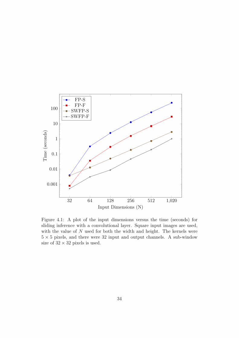
The first relationship to be analysed is how the input image size impacts

the performance of each algorithm. This was accomplished by fixing the

other network hyperparameters, varying the input image size, and applying

the four inference algorithms of interest. The results of this experiment are

given in Figure 4.1. The rate at which the execution time grows for FP-S

and FP-F clearly eliminates the possibility of using either of these algorithms

for real-time applications, whereas the speed of the other two methods looks

quite promising. For a 1024× 1024 pixel input image SWFP-S and SWFP-F

take 2.78 seconds and 0.991 seconds respectively. While this still does not

meet real-time constraints in most scenarios, SWFP-F takes 0.189 seconds to

process a 512× 512 input image which could be sufficient for some real-time

applications.

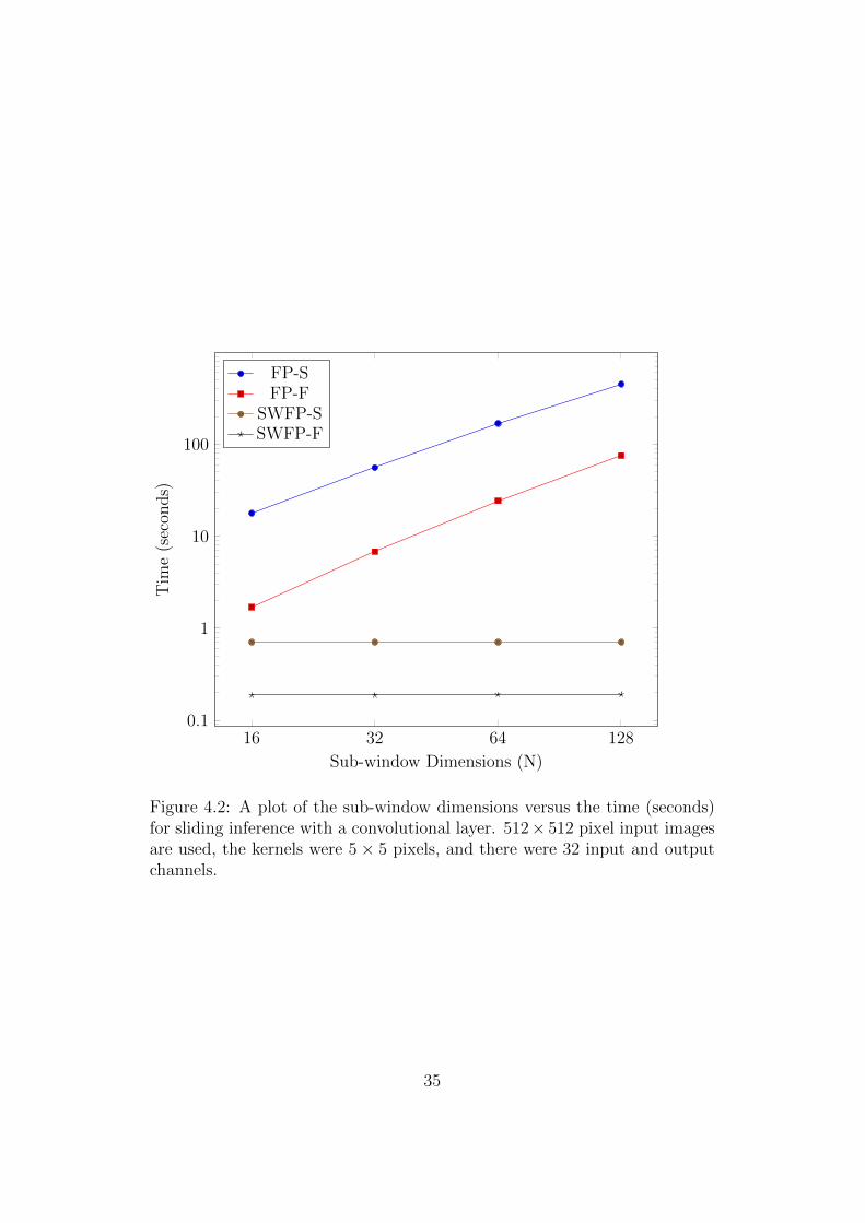
An interesting property of the fast sliding window algorithms, SWFP-S and

SWFP-F, is that neither of their worst case time complexities depend on

the size of the sub-window. However, the algorithms that follow the conven-

tional approach of extracting each sub-window separately do depend on the

window size. To demonstrate the effect that the sub-window size has on the

performance of these algorithms the previous experiment was repeated with

the input image size fixed at 512× 512 pixels, and the sub-window size was

varied instead. The results of this experiment are presented in Figure 4.2.

As expected, the performance of the two algorithms specialised for sliding

window classification exhibit no change in speed as the sub-window size is

changed, and the inverse happens for the two algorithms that are not spe-

cialised for sliding window classification. For a sub-window size of 128× 128

pixels SWFP-F is over 2,000 times faster than FP-S and almost 400 times

faster than FP-F.

Finally, the impact of unrolling the loops in the fully connected layers spe-

cialised for sliding window classification is investigated. This is explored by

evaluating how performance changes when the input image grows, while the

other network hyperparameters remain fixed. 32 input and output channels

were used for this experiment, and the input image size varied from 32 to

1024. Figure 4.3 shows the relative speedup of the fully connected layer with

33

32 64 128 256 512 1,020

0.001

0.01

0.1

1

10

100

Input Dimensions (N)

Tim

e(s

econ

ds)

FP-SFP-F

SWFP-SSWFP-F

Figure 4.1: A plot of the input dimensions versus the time (seconds) forsliding inference with a convolutional layer. Square input images are used,with the value of N used for both the width and height. The kernels were5 × 5 pixels, and there were 32 input and output channels. A sub-windowsize of 32× 32 pixels is used.

34

16 32 64 1280.1

1

10

100

Sub-window Dimensions (N)

Tim

e(s

econ

ds)

FP-SFP-F

SWFP-SSWFP-F

Figure 4.2: A plot of the sub-window dimensions versus the time (seconds)for sliding inference with a convolutional layer. 512× 512 pixel input imagesare used, the kernels were 5× 5 pixels, and there were 32 input and outputchannels.

35

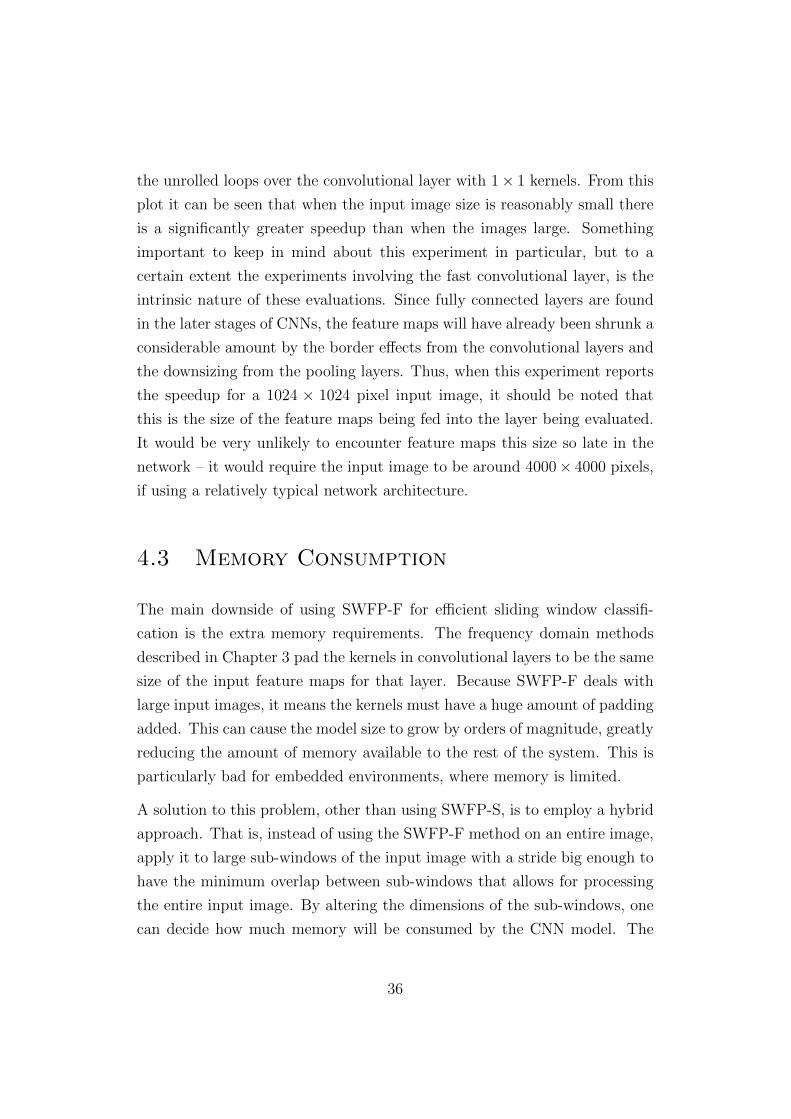
the unrolled loops over the convolutional layer with 1× 1 kernels. From this

plot it can be seen that when the input image size is reasonably small there

is a significantly greater speedup than when the images large. Something

important to keep in mind about this experiment in particular, but to a

certain extent the experiments involving the fast convolutional layer, is the

intrinsic nature of these evaluations. Since fully connected layers are found

in the later stages of CNNs, the feature maps will have already been shrunk a

considerable amount by the border effects from the convolutional layers and

the downsizing from the pooling layers. Thus, when this experiment reports

the speedup for a 1024 × 1024 pixel input image, it should be noted that

this is the size of the feature maps being fed into the layer being evaluated.

It would be very unlikely to encounter feature maps this size so late in the

network – it would require the input image to be around 4000× 4000 pixels,

if using a relatively typical network architecture.

4.3 Memory Consumption

The main downside of using SWFP-F for efficient sliding window classifi-

cation is the extra memory requirements. The frequency domain methods

described in Chapter 3 pad the kernels in convolutional layers to be the same

size of the input feature maps for that layer. Because SWFP-F deals with

large input images, it means the kernels must have a huge amount of padding

added. This can cause the model size to grow by orders of magnitude, greatly

reducing the amount of memory available to the rest of the system. This is

particularly bad for embedded environments, where memory is limited.

A solution to this problem, other than using SWFP-S, is to employ a hybrid

approach. That is, instead of using the SWFP-F method on an entire image,

apply it to large sub-windows of the input image with a stride big enough to

have the minimum overlap between sub-windows that allows for processing

the entire input image. By altering the dimensions of the sub-windows, one

can decide how much memory will be consumed by the CNN model. The

36

32 64 128 256 512 1,0201

2

3

4

5

6

7

8

Input Dimensions

Sp

eedup

Relative Speedup

Figure 4.3: A plot of the relative speedup of the unrolled sliding windowfully connected layer over using a space domain convolutional layer with1× 1 kernels.

37

downside to this approach is that the algorithm will now exhibit a slowdown,

due to redundant calculations being performed where the sub-windows over-

lap.

38

Chapter 5

Applications

“Anyone can build a fast CPU. The trick is to build a fast system.”

— Seymour Cray

This aim of this chapter is to provide an indication of how the algorithms

perform in real world scenarios, as opposed measuring how the layers per-

form in isolation. A selection of classification and object detection tasks are

presented to in order to compare and contrast the execution time for the dif-

ferent training and inference procedures given in Chapter 3 and Chapter 4.

To show that the CNNs used in this chapter can actually be used in practice

the accuracy achieved by each network is also reported, however the primary

motive for providing these applications is to demonstrate how the algorithms

compare in terms of execution speed.

5.1 Classification

Image classification is by far the most common application of CNN mod-

els, which is unsurprising since the motivation for their development was

39

to improve the accuracy of hand written digit recognition [24]. In order

to supply evidence supporting the correctness of the implementation devel-

oped for this project several different networks have been trained on publicly

available image datasets. In addition to reporting how the classification ac-

curacy achieved by the implementation described in Section 3.3, the time

taken per epoch of training when using both frequency domain and spatial

domain algorithms is measured. In the interests of demonstrating how the

frequency domain training procedure compares with the traditional spatial

domain methods in a wide variety of scenarios, the networks selected for

each dataset have very different architectures. This provides a good extrin-

sic performance evaluation that complements the intrinsic evaluation given

in Chapter 3.

5.1.1 MNIST

MNIST is one of the most commonly used datasets for demonstrating image

classification algorithms, particularly those based on CNNs. It consists of

70,000 images of hand written digits that are 28×28 pixels, with a predefined

split of 60,000 training images and 10,000 test images. The images in the

dataset are preprocessed to have the background removed and the digits are

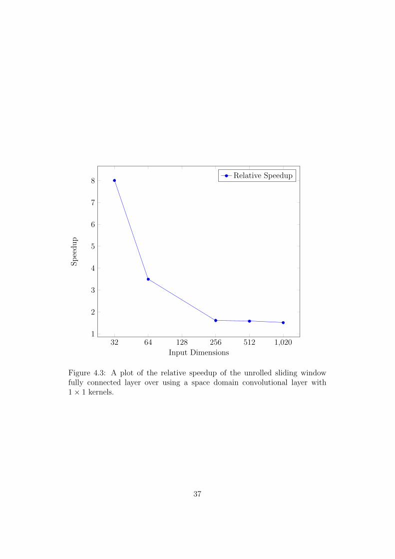
contained in the central 20× 20 pixels of each image. Figure 5.1 shows some

sample images from MNIST.

The network chosen for this dataset was designed by [25], and differs from the

other networks used in this chapter because it only has a single convolutional

layer. Unfortunately not all the details of the network are supplied; there is

no information about the learning rate used, which activation functions are

used in each layer, or details about the weight update rule used. The choice

was made to use rectified linear units in the convolutional layer, and softmax

for the fully connected output layer. A learning rate of 0.01 was used for the

first 20 epochs, and then 0.001 for the next 10 epochs. A momentum rate of

0.9 was used for the entire training process, and SGD was used for the update

rule. These model hyperparameters were found through experimentation on

40

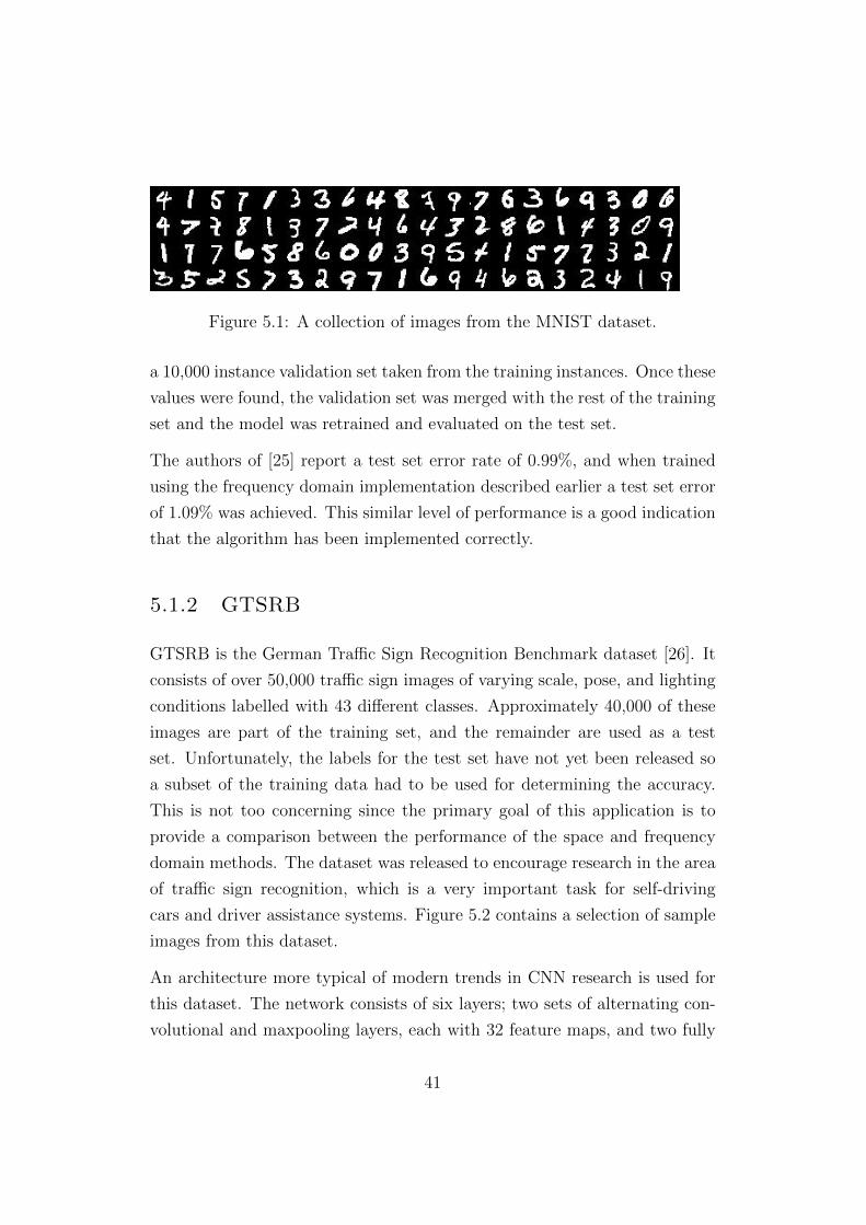
Figure 5.1: A collection of images from the MNIST dataset.

a 10,000 instance validation set taken from the training instances. Once these

values were found, the validation set was merged with the rest of the training

set and the model was retrained and evaluated on the test set.

The authors of [25] report a test set error rate of 0.99%, and when trained

using the frequency domain implementation described earlier a test set error

of 1.09% was achieved. This similar level of performance is a good indication

that the algorithm has been implemented correctly.

5.1.2 GTSRB

GTSRB is the German Traffic Sign Recognition Benchmark dataset [26]. It

consists of over 50,000 traffic sign images of varying scale, pose, and lighting

conditions labelled with 43 different classes. Approximately 40,000 of these

images are part of the training set, and the remainder are used as a test

set. Unfortunately, the labels for the test set have not yet been released so

a subset of the training data had to be used for determining the accuracy.

This is not too concerning since the primary goal of this application is to

provide a comparison between the performance of the space and frequency

domain methods. The dataset was released to encourage research in the area

of traffic sign recognition, which is a very important task for self-driving

cars and driver assistance systems. Figure 5.2 contains a selection of sample

images from this dataset.

An architecture more typical of modern trends in CNN research is used for

this dataset. The network consists of six layers; two sets of alternating con-

volutional and maxpooling layers, each with 32 feature maps, and two fully

41

Figure 5.2: A collection of images from the GTSRB dataset.

connected layers – the first with 32 units and the second with 43 units. A

learning rate of 0.001, momentum of 0.9, and L2 penalty of 0.0001 is used for

all layers. Additionally, the length of each weight vector is constrained to be

less than 3.0. Rectified linear units are used in all layers except the output

layer, where softmax is used. After training for 30 epochs on 35,000 of the

training instances, a validation accuracy of 98.6% is achieved.

5.1.3 CIFAR-10

CIFAR-10 [27] is a 60,000 image subset of the 80 Million Tiny Images dataset [28]

consisting of 10 classes. Under the standard protocol, 50,000 of the images

are used as training data and the remaining 10,000 are used for testing. Over

recent years it has replaced MNIST as the standard dataset for demonstrat-

ing advances in neural network methods. A sample of the instances can be

seen in Figure 5.3. To reduce the problem of overfitting, the training set was

doubled in size by adding the horizontal reflections of the existing training

instances, resulting in a training set of 100,000 instances.

The network used for this dataset is much larger than the previous two

networks, and the volume of data used for training is significantly larger

as well. The CNN consists of two alternating convolutional and maxpooling

layers, followed by two fully connected layers. Both convolutional layers have

64 output feature maps and use 5 × 5 pixel kernels, the maxpooling layers

both use 2×2 pools, and the two fully connected layers have 64 and 10 units

42

Figure 5.3: A collection of images from the CIFAR-10 dataset. Source:http://www.cs.toronto.edu/~kriz/cifar.html

respectively. Once again, rectified linear units are used for all the hidden

layers and the output layer uses the softmax activation function. The network

was trained for 25 epochs with a learning rate of 0.001, which was lowered

to 0.0001 after epoch 15 and 0.00001 after epoch 20. A momentum rate of

0.9 was used for the entire training process. These values were determined

using a validation set drawn from the training set. When the entire training

set was used to build the model an accuracy of 78.3% was achieved on the

test set.

5.1.4 Extrinsic Performance Evaluation

The rigorous intrinsic performance evaluation conducted in Chapter 3 gave a

good indication of the relative performance of the different convolutional layer

algorithms in isolation. That is, the experiments gave performance results

for only a single layer. This section aims to provide an extrinsic performance

evaluation that shows how the execution speed of the spatial and frequency

domain algorithms compare when applied to an entire network being used

43

for image classification. In addition to comparing the training time for the

frequency domain and the space domain methods, measurements are also

reported for unvectorised and vectorised implementations of these algorithms.

The experiments were run on the same system used during Chapter 3 and

the average time taken to train on batches of 10,000 instances is given. Fig-

ure 5.4 shows the execution speed of the four different implementations on

the MNIST, GTSRB, and CIFAR-10 networks.

From the MNIST benchmark it can be seen that a fairly small relative

speedup of the frequency domain methods over the spatial domain methods

has been achieved. This is because the network used was very shallow and

contained only a single convolutional layer. The frequency domain methods

focus solely on accelerating the performance of convolutional layers, so one

would expect to see the relative speedup of the frequency domain approach

over the space domain approach improve as a larger fraction of the compu-

tation is dedicated to convolutional layers. The benchmarks for GTSRB and

CIFAR-10 further suggest that this is the case. Both of those networks have

a significantly larger number of convolutional connections, and exhibit a far

greater speedup than the shallow networks – over and order of magnitude

speedup is gained by the frequency domain methods over the space domain

approach.

5.2 Object Detection

Most object detection pipelines consist of several components that perform

distinct tasks:

1. A binary sliding window classifier that gives a preliminary prediction of

whether a given sub-window contains an object of interest or not. The

output of this stage is a set of bounding boxes for potential matches.

2. Sliding window classifiers almost always generate a cluster of positive

predictions when used for detection tasks. This second stage in the

44

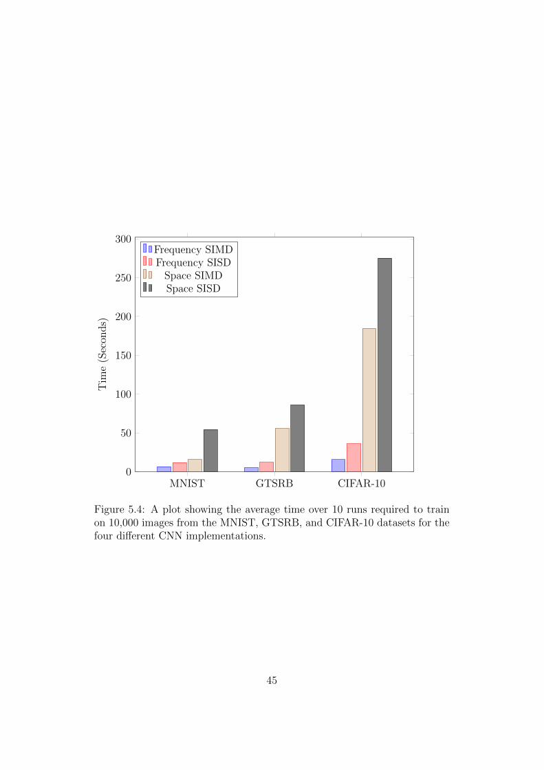
MNIST GTSRB CIFAR-100

50

100

150

200

250

300

Tim

e(S

econ

ds)

Frequency SIMDFrequency SISD

Space SIMDSpace SISD

Figure 5.4: A plot showing the average time over 10 runs required to trainon 10,000 images from the MNIST, GTSRB, and CIFAR-10 datasets for thefour different CNN implementations.

45

pipeline implements a policy for merging overlapping bounding boxes.

3. The sub-windows in the remaining bounding boxes are extracted and

deemed regions of interest.

4. A second classifier is used to review the extracted regions of interest in

order to reduce false positives.

5. The entire process is repeated on several resized copies of the input

image in order to detect objects at multiple scales.

As the focus of this section is the performance of CNNs, the only part of

this object detection pipeline that is inside the scope of this project is the

first stage. As such, it was decided that the only this first stage would

be evaluated, and the accuracy of the network would be measured using a

validation set containing positive and negative examples in isolation. That

is, the accuracy reported is on a hold out set drawn from the same source

as the training data and inference is not performed using sliding window

classification.

The network used for this demonstration consists of two convolutional layers,

each followed by maxpooling layers, and two fully connected layers. Each

of the convolutional and maxpooling layers has 32 feature maps, and the

first and second fully connected layers have 32 and 2 units, respectively.

The network was trained on the German Traffic Sign Detection Benchmark

dataset [29] – not to be confused with the recognition benchmark dataset

released by the same group. All traffic signs and an equal number of negative

examples were randomly extracted from the GTSDB images to generate a

training set. The accuracy achieved by this network is 99.1% on the hold out

set.

5.2.1 Results

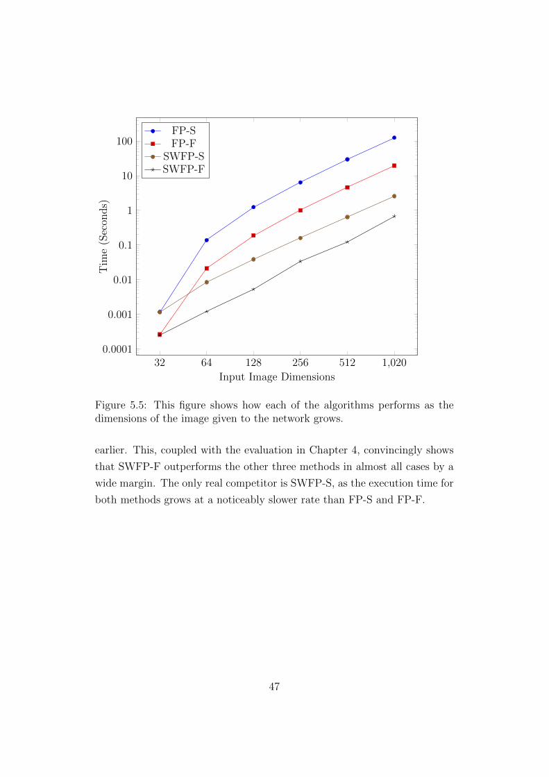
Figure 5.5 gives the average time over 10 runs taken to perform sliding win-

dow classification on images of several sizes using the network described

46

32 64 128 256 512 1,0200.0001

0.001

0.01

0.1

1

10

100

Input Image Dimensions

Tim

e(S

econ

ds)

FP-SFP-F

SWFP-SSWFP-F

Figure 5.5: This figure shows how each of the algorithms performs as thedimensions of the image given to the network grows.

earlier. This, coupled with the evaluation in Chapter 4, convincingly shows

that SWFP-F outperforms the other three methods in almost all cases by a

wide margin. The only real competitor is SWFP-S, as the execution time for

both methods grows at a noticeably slower rate than FP-S and FP-F.

47

Chapter 6

Conclusions

“We can only see a short distance ahead, but we can see plenty there that

needs to be done.”

— Alan Turing

The results that have been presented clearly show that the performance of

training, inference, and sliding window classification with CNNs can be ac-

celerated significantly through the use of frequency domain methods. This

work finishes with a summary of the results and contributions made, as well

as suggestions for future research that could be carried out in this area.

6.1 Summary

The results presented in Chapters 3, 4, and 5 show that frequency domain

methods are significantly faster for performing training, inference, and sliding

window classification operations on CNNs. In cases where computations

involving convolutional layers consume a large fraction of the run time of a

system, these frequency domain methods can be over an order of magnitude

48

faster than the conventional space domain approach used by all publicly

available implementations.

The primary contributions of this work are as follows:

1. Algorithms were derived that utilise frequency domain methods to

greater effect than previous work [16, 17], and a rigorous performance

analysis was conducted that also gave an indication of how these meth-

ods compare to space domain methods in practical applications;

2. A generalisation of CNNs to tensors of arbitrary rank was presented and

formulated in such a way that the fast frequency domain methods can

be applied, improving performance for a much wider range of situations

than just image classification;

3. Sliding window classification was accelerated using a combination of

frequency domain methods and an observation previously made by [23].

In addition to this, the performance of the original fast sliding window

inference algorithm that used space domain methods was quantified;

4. The algorithms described in this work have been implemented in C++

and released as open source.1

6.2 Future Work

There are a multitude of ways in which this work can be further improved

upon. This section describes several possible directions that could be taken:

1. Early experiments showed that the memory throughput of the com-

puter system used for running the benchmarks was being saturated.

Later, it was discovered that the required memory throughput is highly

dependent on the structure of the network, with deep networks being

compute bound, as opposed to memory bound. This suggests that

multi-threading would be a good way to improve performance further;

1Available from http://github.com/henrygouk/nnet

49

2. Many popular CNN implementations utilise the GPGPU paradigm of

computation, through the use of CUDA [4, 30]. Investigating how well

these improved frequency domain methods generalise to GPUs and even

other, more esoteric, architectures would be interesting;

3. Run-time code generation has the potential to have a positive impact

on performance by generating machine code that is optimised for a

particular network structure. Control instructions could be removed

by dynamically unrolling some loops;

4. The fast sliding window method can be further improved upon when

computing dense output maps (i.e., using a stride of 1 for the sliding

window) by representing the layers in the network as a tree with many

duplicated subtrees. In this case each branch in the tree would represent

a different translation of the internal feature maps that are propagated

between layers. The result of this would be that fewer translations

need to be propagated through the earlier layers of the network than

the later layers.

50

Bibliography

[1] D. H. Hubel and T. N. Wiesel, “Receptive fields, binocular interaction

and functional architecture in the cat’s visual cortex,” The Journal of

physiology, vol. 160, no. 1, p. 106, 1962.

[2] K. Hornik, M. Stinchcombe, and H. White, “Multilayer feedforward

networks are universal approximators,” Neural networks, vol. 2, no. 5,

pp. 359–366, 1989.

[3] Q. V. Le, M. Ranzato, R. Monga, M. Devin, K. Chen, G. S. Corrado,

J. Dean, and A. Y. Ng, “Building high-level features using large scale

unsupervised learning,” arXiv preprint arXiv:1112.6209, 2011.

[4] A. Krizhevsky, I. Sutskever, and G. Hinton, “Imagenet classification

with deep convolutional neural networks,” in Advances in Neural Infor-

mation Processing Systems 25, pp. 1106–1114, 2012.

[5] J. Ngiam, A. Coates, A. Lahiri, B. Prochnow, A. Ng, and Q. V. Le,

“On optimization methods for deep learning,” in Proceedings of the 28th

International Conference on Machine Learning (ICML-11), pp. 265–272,

2011.

[6] Y. Nesterov, “A method of solving a convex programming problem with

convergence rate O(1/k2),” in Soviet Mathematics Doklady, vol. 27,

pp. 372–376, 1983.

[7] Y. LeCun, L. Bottou, G. Orr, and K. Muller, “Efficient backprop,” in

Neural Networks: Tricks of the trade (G. Orr and M. K., eds.), Springer,

51

1998.

[8] I. Sutskever, J. Martens, G. Dahl, and G. Hinton, “On the importance

of initialization and momentum in deep learning,” in Proceedings of the

30th International Conference on Machine Learning (ICML-13), vol. 28,

pp. 1139–1147, 2013.

[9] T. Schaul, S. Zhang, and Y. LeCun, “No more pesky learning rates,”

in Proc. International Conference on Machine learning (ICML’13),

pp. 343–351, 2013.

[10] M. Riedmiller and H. Braun, “RPROP - A fast adaptive learning al-

gorithm,” in Proceedings of the International Symposium on Computer

and Information Science VII), 1992.

[11] R. A. Jacobs, “Increased rates of convergence through learning rate

adaptation,” Neural networks, vol. 1, no. 4, pp. 295–307, 1988.

[12] D. C. Ciresan, U. Meier, J. Masci, L. M. Gambardella, and J. Schmid-

huber, “Flexible, high performance convolutional neural networks for

image classification,” in Proceedings of the Twenty-Second international

joint conference on Artificial Intelligence, pp. 1237–1242, AAAI Press,

2011.

[13] R. Uetz and S. Behnke, “Large-scale object recognition with cuda-

accelerated hierarchical neural networks,” in Intelligent Computing and

Intelligent Systems, 2009. ICIS 2009. IEEE International Conference

on, vol. 1, pp. 536–541, IEEE, 2009.

[14] C. Farabet, C. Poulet, J. Y. Han, and Y. LeCun, “CNP: An FPGA-based

processor for convolutional networks,” in Field Programmable Logic and

Applications, 2009. FPL 2009. International Conference on, pp. 32–37,

IEEE, 2009.

[15] C. Farabet, B. Martini, P. Akselrod, S. Talay, Y. LeCun, and E. Cu-

lurciello, “Hardware accelerated convolutional neural networks for syn-

thetic vision systems,” in Circuits and Systems (ISCAS), Proceedings of

2010 IEEE International Symposium on, pp. 257–260, IEEE, 2010.

52

[16] H. Gouk, “Accelerating Convolutional Neural Networks,” tech. rep., De-

partment of Computer Science, University Of Waikato, 2013.

[17] M. Mathieu, M. Henaff, and Y. LeCun, “Fast Training of Convolutional

Networks through FFTs,” arXiv preprint arXiv:1312.5851, 2013.

[18] J. Deng, W. Dong, R. Socher, L.-J. Li, K. Li, and L. Fei-Fei, “Imagenet:

A large-scale hierarchical image database,” in Computer Vision and Pat-

tern Recognition, 2009. CVPR 2009. IEEE Conference on, pp. 248–255,

IEEE, 2009.

[19] L. Deng, O. Abdel-Hamid, and D. Yu, “A deep convolutional neural

network using heterogeneous pooling for trading acoustic invariance

with phonetic confusion,” in Acoustics, Speech and Signal Processing

(ICASSP), 2013 IEEE International Conference on, pp. 6669–6673,

2013.

[20] S. Ji, W. Xu, M. Yang, and K. Yu, “3d convolutional neural networks for

human action recognition,” Pattern Analysis and Machine Intelligence,

IEEE Transactions on, vol. 35, no. 1, pp. 221–231, 2013.

[21] A. M. Blake, I. H. Witten, and M. J. Cree, “The fastest Fourier trans-

form in the south,” IEEE Transactions on Signal Processing, vol. 61,

no. 17-20, pp. 4707–4716, 2013.

[22] M. Frigo and S. G. Johnson, “The design and implementation of

FFTW3,” Proceedings of the IEEE, vol. 93, no. 2, pp. 216–231, 2005.

Special issue on “Program Generation, Optimization, and Platform

Adaptation”.

[23] P. Sermanet, D. Eigen, X. Zhang, M. Mathieu, R. Fergus, and Y. Le-

Cun, “Overfeat: Integrated recognition, localization and detection using

convolutional networks,” arXiv preprint arXiv:1312.6229, 2013.

[24] Y. LeCun, B. Boser, J. S. Denker, D. Henderson, R. E. Howard, W. Hub-

bard, and L. D. Jackel, “Backpropagation applied to handwritten zip

code recognition,” Neural Computation, vol. 1, pp. 541–551, Winter

1989.

53

[25] D. Scherer, A. Muller, and S. Behnke, “Evaluation of pooling opera-

tions in convolutional architectures for object recognition,” in Artificial

Neural Networks–ICANN 2010, pp. 92–101, Springer, 2010.

[26] J. Stallkamp, M. Schlipsing, J. Salmen, and C. Igel, “Man vs. computer:

Benchmarking machine learning algorithms for traffic sign recognition,”

Neural Networks, 2012.

[27] A. Krizhevsky and G. Hinton, “Learning multiple layers of features from

tiny images,” tech. rep., Computer Science Department, University of

Toronto, 2009.

[28] A. Torralba, R. Fergus, and W. T. Freeman, “80 million tiny images:

A large data set for nonparametric object and scene recognition,” Pat-

tern Analysis and Machine Intelligence, IEEE Transactions on, vol. 30,

no. 11, pp. 1958–1970, 2008.

[29] S. Houben, J. Stallkamp, J. Salmen, M. Schlipsing, and C. Igel, “Detec-

tion of traffic signs in real-world images: The German Traffic Sign De-

tection Benchmark,” in International Joint Conference on Neural Net-

works, pp. 1–8, 2013.

[30] J. Bergstra, F. Bastien, O. Breuleux, P. Lamblin, R. Pascanu, O. De-

lalleau, G. Desjardins, D. Warde-Farley, I. Goodfellow, A. Bergeron,

et al., “Theano: Deep learning on gpus with python,” in NIPS 2011,

BigLearning Workshop, Granada, Spain, 2011.

54

Appendices

55

Appendix A

Multi-Dimensional Algorithms

A number of algorithms are required to manipulate signal in arbitrary dimen-

sions. They are mostly variants of cropping and padding operations, with

rotating happening at the same time to reduce the number of passes over

memory required. Pseudocode for these algorithms is given here.

56

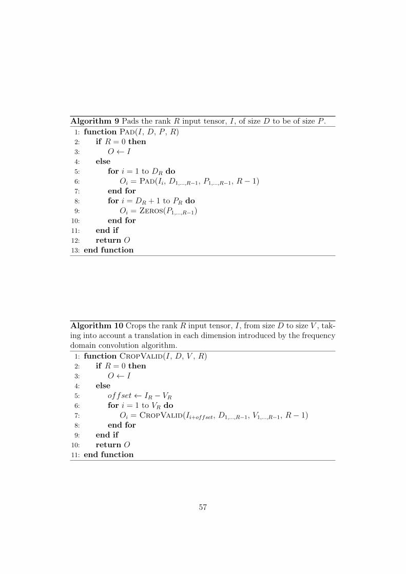
Algorithm 9 Pads the rank R input tensor, I, of size D to be of size P .

1: function Pad(I, D, P , R)2: if R = 0 then3: O ← I4: else5: for i = 1 to DR do6: Oi = Pad(Ii, D1,...,R−1, P1,...,R−1, R− 1)7: end for8: for i = DR + 1 to PR do9: Oi = Zeros(P1,...,R−1)

10: end for11: end if12: return O13: end function

Algorithm 10 Crops the rank R input tensor, I, from size D to size V , tak-ing into account a translation in each dimension introduced by the frequencydomain convolution algorithm.

1: function CropValid(I, D, V , R)2: if R = 0 then3: O ← I4: else5: offset← IR − VR6: for i = 1 to VR do7: Oi = CropValid(Ii+offset, D1,...,R−1, V1,...,R−1, R− 1)8: end for9: end if

10: return O11: end function

57

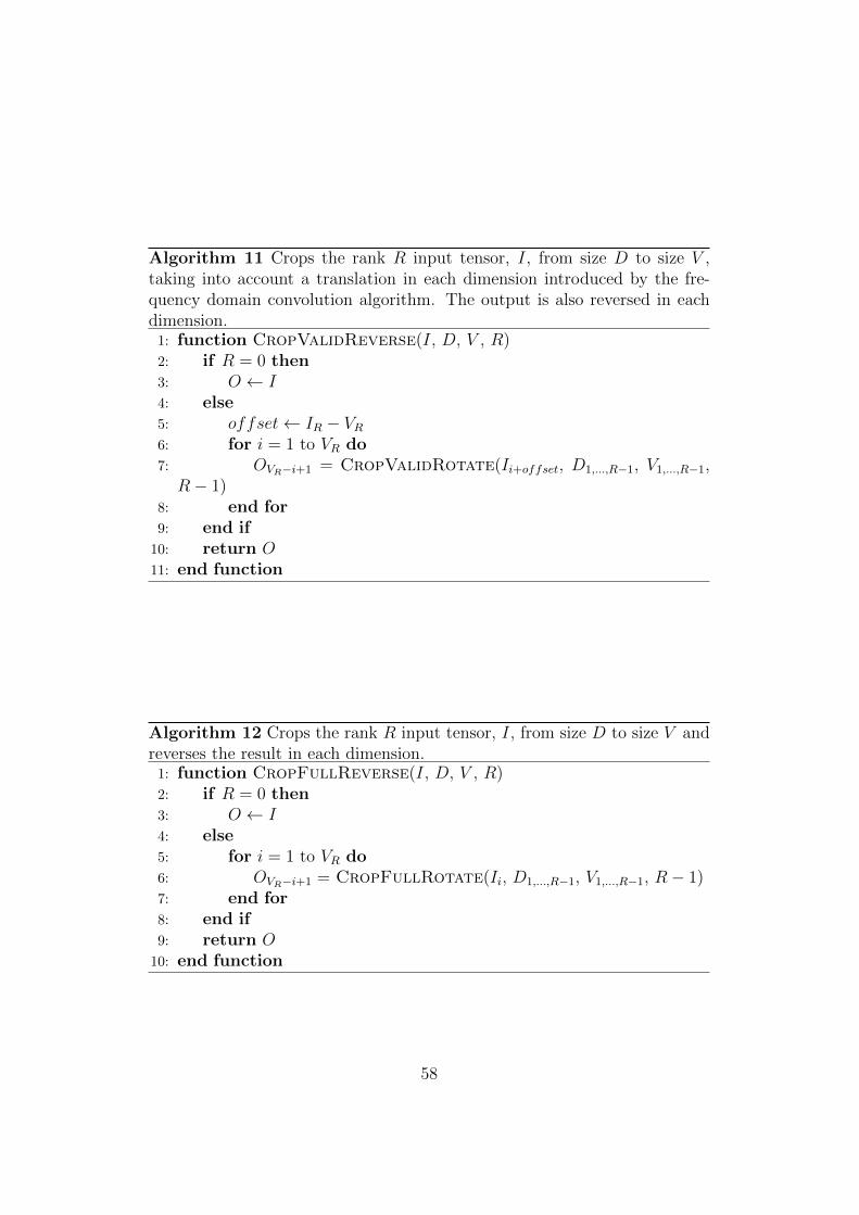
Algorithm 11 Crops the rank R input tensor, I, from size D to size V ,taking into account a translation in each dimension introduced by the fre-quency domain convolution algorithm. The output is also reversed in eachdimension.1: function CropValidReverse(I, D, V , R)2: if R = 0 then3: O ← I4: else5: offset← IR − VR6: for i = 1 to VR do7: OVR−i+1 = CropValidRotate(Ii+offset, D1,...,R−1, V1,...,R−1,

R− 1)8: end for9: end if

10: return O11: end function

Algorithm 12 Crops the rank R input tensor, I, from size D to size V andreverses the result in each dimension.1: function CropFullReverse(I, D, V , R)2: if R = 0 then3: O ← I4: else5: for i = 1 to VR do6: OVR−i+1 = CropFullRotate(Ii, D1,...,R−1, V1,...,R−1, R− 1)7: end for8: end if9: return O

10: end function

58

Appendix B

Efficient Complex

Multiplication

Great care was taken to optimise the complex multiply and accumulate rou-

tine used due the procedure taking up a very large fraction of the overall

runtime – particularly in larger networks. The following code shows how this

was accomplished using AVX instructions.

s t a t i c i n l i n e m256 VCFMA( m256 c , m256 a , m256 b)

{m256 b f l i p = mm256 shuf f l e ps (b , b , 0 xB1 ) ;

m256 a r e = mm256 shuf f l e ps ( a , a , 0 xA0 ) ;

m256 a im = mm256 shuf f l e ps ( a , a , 0 xF5 ) ;

m256 arb = mm256 fmadd ps ( a re , b , c ) ;

m256 aib = mm256 mul ps ( a im , b f l i p ) ;

r e turn mm256 addsub ps ( arb , a ib ) ;

}

59