exploiting parallelism in matrix-computation kernels for ...paolo/reference/dalbertobn2011.pdf ·...

-

Exploiting Parallelism in Matrix-Computation Kernels for SymmetricMultiprocessor SystemsMatrix-Multiplication and Matrix-Addition Algorithm Optimizations by Software Pipeliningand Threads Allocation

Paolo D’Alberto, Yahoo! Sunnivale, CA, USAMarco Bodrato, University of Rome II, Tor Vergata, ItalyAlexandru Nicolau, University of California at Irvine, USA

We present a simple and efficient methodology for the development, tuning, and installation of matrix al-gorithms such as the hybrid Strassen’s and Winograd’s fast matrix multiply or their combination with the3M algorithm for complex matrices (i.e., hybrid: a recursive algorithm as Strassen’s until a highly tunedBLAS matrix multiplication allows performance advantages). We investigate how modern symmetric multi-processor (SMP) architectures present old and new challenges that can be addressed by the combination ofan algorithm design with careful and natural parallelism exploitation at the function level (optimizations)such as function-call parallelism, function percolation, and function software pipelining.

We have three contributions: first, we present a performance overview for double and double complexprecision matrices for state-of-the-art SMP systems; second, we introduce new algorithm implementations: avariant of the 3M algorithm and two new different schedules of Winograd’s matrix multiplication (achievingup to 20% speed up w.r.t. regular matrix multiplication). About the latter Winograd’s algorithms: one isdesigned to minimize the number of matrix additions and the other to minimize the computation latency ofmatrix additions; third, we apply software pipelining and threads allocation to all the algorithms and weshow how that yields up to 10% further performance improvements.

Categories and Subject Descriptors: G.4 [Mathematics of Computing]: Mathematical Software; D.2.8[Software Engineering]: Metrics—complexity measures, performance measures; D.2.3 [Software Engi-neering]: Coding Tools and Techniques—Top-down programming

Additional Key Words and Phrases: Matrix Multiplications, Fast Algorithms, Software Pipeline, Parallelism

ACM Reference Format:D’Alberto, P., Bodrato, M., and Nicolau, A. 2011. Exploiting Parallelism in Matrix-Computation Kernels forSymmetric Multiprocessor Systems. ACM Trans. Embedd. Comput. Syst. -, -, Article - ( 2011), 30 pages.DOI = 10.1145/0000000.0000000 http://doi.acm.org/10.1145/0000000.0000000

1. INTRODUCTIONMulticore multiprocessor blades are the most common computational and storagenodes in data centers, multi-nodes are becoming the trend (a blade supporting oneor two boards), and mixed systems based on the Cell processor are topping the fastest-supercomputers list.

In this work, we experiment with general purpose processors; this type of nodeis often used in search-engine data centers, it can reach up to 200 Giga FLOPS(i.e., depending on the number of processors and CPU’s frequency; for example, we

Email the authors: Paolo D’Alberto [email protected], Marco Bodrato [email protected],Alexandru Nicolau [email protected], for request a copy of the code [email protected] to make digital or hard copies of part or all of this work for personal or classroom use is grantedwithout fee provided that copies are not made or distributed for profit or commercial advantage and thatcopies show this notice on the first page or initial screen of a display along with the full citation. Copyrightsfor components of this work owned by others than ACM must be honored. Abstracting with credit is per-mitted. To copy otherwise, to republish, to post on servers, to redistribute to lists, or to use any componentof this work in other works requires prior specific permission and/or a fee. Permissions may be requestedfrom Publications Dept., ACM, Inc., 2 Penn Plaza, Suite 701, New York, NY 10121-0701 USA, fax +1 (212)869-0481, or [email protected]© 2011 ACM 1539-9087/2011/-ART- $10.00

DOI 10.1145/0000000.0000000 http://doi.acm.org/10.1145/0000000.0000000

ACM Transactions on Embedded Computing Systems, Vol. -, No. -, Article -, Publication date: 2011.

-:2 P. D’Alberto, M. Bodrato, A. Nicolau

will present a system providing 150 GFLOPS in practice in single precision and 75GFLOPS in double precision), and such nodes can (and do) serve as the basis for quitecomplex parallel architectures. These machines implement a shared memory system sothat developers may use the PRAM model as an abstraction (e.g., [JaJa 1992]). Thatis, developers think and design algorithms as a collaboration among tasks withoutexplicit communications by using the memory for data sharing and data communica-tions.

In this work, we investigate the implementation features and performance caveatsof fast matrix-multiplication algorithms: the hybrid Strassen’s, Winograd’s, and 3Mmatrix multiplications algorithms (the last is for complex matrices). For example, thehybrid Winograd’s matrix multiplication is a recursive algorithm deploying the Wino-grad’s algorithm using 15 matrix addition in place of a (recursive) matrix multiplica-tion until —the size of the operand matrices are small enough so that— we can deploya highly tuned BLAS matrix multiplication implementation so that to achieve the bestperformance. These algorithms are a means for a fast implementation of matrix multi-plication (MM). Thus, we present optimizations at algorithmic level, thread allocationlevel, function scheduling level, register allocation level, and instruction schedulinglevel so as to improve these MM algorithms, which are basic kernels in matrix compu-tations. However, we look at them as an example of matrix-computations on top of thematrix algebra (*, +). As such, we think the concepts introduced and applied in thiswork are of more general interests. Our novel contributions are:

(1) We present new algorithms that are necessary for the next contributions and op-timizations (the following optimization in the paper). Here, we present optimiza-tions that when applied to the-state-of-the-art algorithms A provide a speed up of,let us say, 2–5%. To have full effect of our optimizations we need to formulate anew family of algorithms B, though these algorithms are slower than the ones inA. When we apply our optimizations in a parallel architecture to the algorithmsin B, we may achieve even better performance, for example, 10–15% w.r.t. A. Dur-ing the discovery of the algorithms in B, we have found and present another classof algorithms C that are faster than A (up to 2% faster) but when we apply ouroptimizations these algorithms achieve a speed up of only 5–7% w.r.t. A.

(2) We show that these fast algorithms are compelling for a large set of SMP systems:they are fast, simple to code and maintain.

(3) We show that fast algorithms offer a much richer scenario and more opportunitiesfor optimizations than the classical MM implementation. Actually, we show thatwe have further space for improvements (10–15%) making fast algorithms evenfaster than we have already shown in previous implementations. In practice, atthe fast-algorithms core is the trade off between MMs and matrix additions MAs(trading one MM for a few MAs). In this paper, we propose a new approach toscheduling, and thread allocation for MA and MM in the context of fast MM, andwe explore and measure the advantages of these new techniques. As a side ef-fect, we show that thanks to parallelism we can speed up the original Strassen’salgorithm such that it can be as fast as the Winograd’s formulation and we canimplement the resulting algorithm in such a way as to achieve the ideal speed upw.r.t. highly tune implementations of MM. That is, We have found an operationschedule that hides the MAs latency completely; thus, we reduce or nullify the per-formance influence of the number of MAs and, thus, achieving the ideal speedupsthat Winograd/Strassen algorithms could achieve.In Figure 1, we show graphically a summary of the best possible speed up we canachieve using Winograd’s algorithms and our optimizations (GotoBLAS DGEMMis the reference).


Exploiting Parallelism in Matrix-Computation Kernels -:3

0

5

10

15

20

25

Pen)um4cores Opteron4cores Xeon8cores Shanghai8cores Nehalem16cores

%speedupw.r.t.GotoBLAS

ParallelWinograd+Pipelining

ParallelWinograd

Fig. 1. Summary: speed up w.r.t. GotoBLAS double precision for a few systems. GotoBLAS has speed up 1

(4) We believe this work could be of interest for compiler designers and developersfrom other fields. At first, our contribution seems limited to fast algorithms, but inpractice, what we propose is applied to matrix computations build on the matrixalgebra (*,+) composed of parallel basic MM (*) and MA (+) subroutines (i.e., matrixcomputations are simply a sequence of * and + operations and the optimizationswe propose could be applied to any such schedules).

In practice, we present a family of fast algorithms that can achieve an ideal speedup w.r.t. the state-of-the-art algorithms such as the ones available in GotoBLAS andATLAS library (i.e., one recursion level of Strasswe/Winograd algorithm will be 8/7faster than GotoBLAS GEMM). The introduction of our optimizations and algorithmsprovide speed up that other implementations of Winograd’s algorithm —based onlyon algorithmic improvements without taking in account of the architecture— cannotmatch nor outperform. For any machine where a fast implementation (not using ourtechniques) is available, our approach can derive a significantly faster algorithm usingthis BLAS implementation as building block (leaf).

The paper is organized as follows. In Section 2, we introduce the related work. InSection 3, we introduce the notations and matrix computation algorithms such as MMand MA. In Section 4, we introduce the fast algorithms and thus our main contri-butions. In Section 6, we introduce our experiments and divide them into single anddouble precision sections (thus single and double complex).

2. RELATED WORKOur main interest is the design and implementation of highly portable codes that au-tomatically adapt to the architecture evolution, that is, adaptive codes (e.g., [Frigoand Johnson 2005; Demmel et al. 2005; Puschel et al. 2005; Gunnels et al. 2001]). Inthis paper, we discuss a family of algorithms from dense linear algebra: Matrix Mul-tiply (MM). All algorithms apply to any size and shape matrices stored in either rowor column-major layout (i.e., our algorithm is suitable for both C and FORTRAN, al-gorithms using row-major order [Frens and Wise 1997; Eiron et al. 1998; Whaley andDongarra 1998], and using column-major order [Higham 1990; Whaley and Dongarra1998; Goto and van de Geijn 2008]).

Software packages such as LAPACK [Anderson et al. 1995] are based on a basicroutine set such as the basic linear algebra subprograms BLAS 3 [Lawson et al. 1979;Dongarra et al. 1990b; 1990a; Blackford et al. 2002]. In turn, BLAS 3 can be built ontop of an efficient implementations of the MM kernel [Kagstrom et al. 1998a; 1998b].ATLAS [Whaley and Dongarra 1998; Whaley and Petitet 2005; Demmel et al. 2005]



Table I. Recursion point (problem size when we yield to GEMM) for a fewarchitectures and for different precisions

machine single double single complex double complexOpteron 3100 3100 1500 1500Pentium 3100 2500 1500 1500Nehalem 3800 3800 2000 2000Xeon 7000 7000 3500 3500Shanghai 3500 3500 3500 3500

(pseudo successor of PHiPAC [Bilmes et al. 1997]) is a very good example of an adaptivesoftware package implementing BLAS, by tuning codes for many architectures arounda highly tuned MM kernel optimized automatically for the L1 and L2 data caches.Recently however, GotoBLAS [Goto and van de Geijn 2008] (or Intel’s MKL or a fewvendor implementations) is offering consistently better performance than ATLAS.

In this paper, we take a step forward towards the parallel implementation of fastMM algorithms: we show how, when, and where our (novel) hybrid implementationsof Strassen’s, Winograd’s, and the 3M algorithms [Strassen 1969; Douglas et al. 1994;D’Alberto and Nicolau 2009; 2007] improve the performance over the best availableadaptive matrix multiply (e.g., ATLAS or GotoBLAS). We use the term fast algo-rithms to refer to the algorithms that have asymptotic complexity less than O(N3),and we use the term classic or conventional algorithms for those that have com-plexity O(N3). We take the freedom to stretch the term fast algorithm in such a way tocomprise the 3M algorithm for complex matrices. Strassen’s algorithm [Strassen 1969]is the first practically used among the fast algorithms for MM.

The asymptotically fastest algorithm to date is by Coppersmith and WinogradO(n2.376) [Coppersmith and Winograd 1987]. Pan showed a bi-linear algorithm that isasymptotically faster than Strassen-Winograd [Pan 1978] O(n2.79) (i.e., see Pan’s sur-vey [Pan 1984] with best asymptotic complexity of O(n2.49)). Kaporin [Kaporin 1999;2004] presented the implementation of Pan’s algorithm O(n2.79). For the range of prob-lem sizes presented in this work, the asymptotic complexity of Winograd’s and Pan’s issimilar. Recently, new, group-theoretic algorithms that have complexity O(n2.41) [Cohnet al. 2005] have been proposed. These algorithms are numerically stable [Demmelet al. 2006] because they are based on the Discrete Fourier Transform (DFT) kernelcomputation. However, there have not been any experimental quantification of thebenefits of such approaches.

In practice, for relatively small matrices, Winograd’s MM has a significant over-head and classic MMs are more appealing. To overcome this, Strassen/Winograd’sMM is used in conjunction with classic MM [Brent 1970b; 1970a; Higham 1990]:for a specific problem size n1, or recursion point [Huss-Lederman et al. 1996],Strassen/Winograd’s algorithm yields the computation to the classic MM implemen-tations. The recursion point depends on various properties of the machine hardware,and thus will vary from one machine to the next.

In table I, we show an excerpt of the possible recursion points for the architecturepresented in this paper. However, the recursion point is immaterial per se because itcan be always estimated and tuned for any architecture and family of problems (e.g.,real or complex).

A practical problem with Strassen and Winograd’s algorithms is how to divide thematrix when not a power of two. All our algorithms divide the MM problems intoa set of balanced subproblems; that is, with minimum difference of operation count(i.e., complexity). This balanced division leads to simple code, and natural recursiveparallelism. This balanced division strategy differs from the division process proposedby Huss-Lederman et al. [Huss-Lederman et al. 1996; Huss-Lederman et al. 1996;



Higham 1990], where the division is a function of the problem size. In fact, for odd-matrix sizes, they divide the problem into a large even-size problem (peeling), on whichStrassen’s algorithm is applied once or recursively, and a few irregular computationsbased on matrix-vector operations.

Recently, there is a new interest in discovering new algorithms (or schedules) aswell as new implementations taken from the Winograd’s MM. Our work is similar tothe ones presented in [Dumas et al. 2008; Boyer et al. 2009] and takes from a con-current work in [Bodrato 2010]. The first presents a library (how to integrate finiteprecision MM computation with high performance double precision MM) and the sec-ond presents new implementations in such a way to minimize the memory space (i.e.,foot print) of Strassen–Winograd’s MM. Memory efficient fast MMs are interesting be-cause the natural reduction of memory space also improves the data locality of thecomputation (extremely beneficial when data spill to disk). The third proposes an op-timized algorithm to reduce even further the computation for matrices of odd sizes.In contrast, in this work, we are going to show that to achieve performance, we needparallelism; to exploit parallelism, we need more temporary space (worse memory footprint). We show that the fastest algorithm (among the ones presented in this work)requires the largest space to allow more parallelism; thus, if we can work in mem-ory without disk spills, we present the best performance strategy, otherwise a hybridapproach is advised.

3. ALGORITHMS DESIGN AND TASKS SCHEDULINGIn this section, we present MM (i.e., the classic one) and MA algorithms and imple-mentations for multicore multiprocessor SMP systems. We present both the main al-gorithms and the optimizations in an intuitive but rigorous way.

Before we present any algorithm, we introduce our notations. Consider any matrixA ∈ Rm×n, this can be always divided into four quadrants:

A =

[A0 A1

A2 A3

](1)

where A0 ∈ Rdm2 e×d

n2 e and A3 ∈ Rbm

2 c×bn2 c. In the same way, we can divide a matrix

into two vertical matrices (similarly horizontal ones):

A =[A0 A1

](2)

where A0 ∈ Rm×dn2 e and A1 ∈ Rm×bn

2 c.

3.1. Classic Matrix Multiplication O(N3)

The classic matrix multiplication (MM) of C=AB with C,A,B ∈ Rn×n is defined bythe following recursive algorithm:

C0=A0B0 + A1B2 C1=A0B1 + A1B3,C2=A2B0 + A3B2 C3=A2B1 + A3B3

(3)

The computation is divided into four parts, one for each sub-matrix composing C.Thus, for every matrix Ci (0 ≤ i ≤ 3), the classic approach computes two products,using a total of 8 MMs and 4 MAs (which can be computed concurrently with MMand thus not contributing to the overall execution time). Notice that every productcomputes a result that has the same size and shape as the destination sub-matrix Ci.If we decide to compute the products recursively, each product AiBj is divided furtherinto four subproblems, and the computation in Equation 3 applies unchanged to thesesubproblems.



The time complexity of MM is 2n3 (n3 multiplications and n3 additions); the spacecomplexity is 3n2 requiring at least the storage of the addenda and the result; the num-ber of memory accesses (if the problem fits in memory) also known as I/O complexityor access complexity is O( n

3√S) where S is the size of the largest cache as a function of

the number of matrix elements; the constant term is a function of how the problem isdivided. 1

The MM procedure has data locality and we can easily parallelize MM using threadson a SMP architecture; for example, Equation 3 presents one policy of how to divide thecomputation. In this work, we deploy either ATLAS or GotoBLAS multi-threaded MMwhere the number of threads (the parallelism) and the core allocation can be drivenby either a few global environment variables or, as in our case, using the Linux utility,set affinity.

3.2. Matrix AdditionMatrix addition (MA) C = A + B with C,A,B ∈ Rn×n, has time complexity O(n2)because it requires n2 additions, 2n2 reads and n2 writes; thus 3n2 memory accessoperations. The MA has space complexity 3n2 because its input and output are threematrices.

The MA does not have temporal locality because any matrix element is used justonce. It has spatial locality; that is, we tend to read and write contiguous elementsfrom/to the matrices. The nonexistent temporal locality makes a hierarchical memory(level of caches) completely useless and actually harmful (we could achieve better per-formance if we just circumvent the caches and go directly to the register files). TheMA is embarrassingly parallel. For example, if we divide a matrix into two verticalsub-matrices we can easily describe the addition as two parallel MAs (Equation 4):

p0C0

p1C1 =

p0A0 + B0

p1A1 + B1

(4)

We can perform this division recursively until we achieve the number of tasks nec-essary and, also, we can determine a logical allocation of each MA to a specificcore/processor. We can time the MA performance for the purpose of investigating thedata throughput to all cores. For example, if the MA performance improves as thenumber of threads increases till matching the number of cores, we can state that thememory system has the bandwidth to provide data to all cores (the computation costis negligible compared to the communication cost). In this work, all architectures canactually feed all cores for computing MA (note this is not necessarily true for other ap-plications such as the classic MM because of the different access complexity). However,notice that even when the memory system has the bandwidth to sustain computationto all cores, it does not means that we can achieve the maximum throughput of anycore.

Remark. to simplify the complexity model and operation counts, in the following,we consider a matrix copy (i.e., A = B) as time consuming as a matrix addition.

3.3. The classic MM and MA algorithm as building blocks for fast algorithmsIn the following, we consider the classic MM and the MA as parallel routines optimizedfor the specific architectures. Our fast matrix multiplication algorithms are writtenas a sequence of these operations (recursive divide-and-conquer algorithms) and wemodel the system simply as the composition of a core set and a single memory storage(i.e., parallel random access memory machine PRAM). We further make sure that: first,

1The recursive division in Equation 3 is not the best but asymptotically optimal nonetheless.



each basic operation is optimized for the architecture achieving optimal/best through-put; second, the problem size is large enough that a parallel system is necessary toobtain results in a timely manner. In the following, we investigate how to integrateand combine MM and MA to optimize the code and improve the performance.

4. FAST MATRIX MULTIPLICATION ALGORITHMSWe present all the following fast MMs as a sequence of MMs and MAs. As such, anyMM can be either a recursive call to a fast MM or a direct call to an optimized and clas-sic BLAS MM (GEMM). A recursive MM algorithm will switch to the classic MM forany problem sizes smaller than a specified threshold or recursion point (we specify inthe set up how this point is computed, Section 6.1). The recursion point is a function ofthe architecture, the implementation of the classic MM algorithm and the implementa-tion of MA. In this work, the recursion point is found empirically for each architectureonce the library is installed. We present four basic hybrid algorithms based on a bal-anced decomposition of the matrix operands: 3M Section 4.1, Strassen’s 4.3 , Winograd4.2, Winograd optimized to reduce MAs (WOPT) 4.4, and Winograd optimized to hideMA latency (WIDEAL) 4.5.

4.1. 3M Matrix Multiply

Table II. 3M algorithm.

Sequential Parallel/Pipelining

CR = ARBR 1: CR = ARBR T = AR + AI S = BR + BI

CI = AIBI 2: CI = AIBI

CI = CI + CR 3: CI = CI + CR

CR = 2CR −CI 4: CR = 2CR −CI

T = AR + AI 5: CI− =STS = BR + BI

CI− = ST

We can consider a complex matrix−A as either a matrix where each element is a

complex number −ak,` = (bk,` + ick,`), or the composition of two real matrices−A =

AR + iAI . If we adopt the former, we can compute the MM by any implementationdiscussed so far. If we adopt the latter, we can use an even faster algorithm: the 3Mmultiplication as in Table II. Our implementation hides the latency of the last MAbecause MA and MM are computed at the same time, and it introduces a small extracomputation because one addition is of the form: CR = 2CR − CI . In practice, thisalgorithm has 3 MM, thus the name of the algorithm, and only four MAs (instead offive).

The MM dominates the overall time complexity. Independently of our real-MM-algorithm choice, the 3M algorithm requires extra space for the temporary matricesT and S (i.e., an extra complex matrix). So at a minimum, the 3M algorithm has aspace complexity of 4n2. If we apply the classic algorithm, the 3M algorithm has thetime complexity of O(3 ∗ 2n3). Due to the data locality, we know that given the largestcache sizes S (e.g., L2 or L3) we have O(3 2n3

√S

) memory accesses. The 3M algorithm—in comparison with the classic MM applied to complex matrices— offers a ∼ 4

3 speedup. This fast algorithm, actually every 3M algorithm, compromises the precision of theimaginary part of the complex result matrix because of the compounding error effectsof both MA and MM similar to the Strassen’s algorithm.



Algorithm and scheduling. We notice that the MAs T = AR+AI and S = BR+BI

can be executed in parallel to the previous addition and actually as early as the firstmatrix multiplications as we suggested in Table II; that is, we perform a functionpercolation (upward movement), in principle as in [Nicolau et al. 2009]. Notice that wedid schedule the two independent MMs CR = ARBR and CI = AIBI into two differentsteps (line 1 and 2) (instead of executing them in parallel together). We do this becauseeach MM will be parallelized and we will achieve the best asymptotic performance foreach multiplication separately, thus there would be no loss of performance.

If the MM cannot exploit full parallelism from an architecture, some cores arebetter running idle than executing small sub problems of MM (because we mayachieve a lower throughput). A MA has the same space complexity of a MM, it hasa (much) smaller time complexity and, more importantly, fewer memory accesses: 3n2

vs. 2n3/√S, where S is the size of the largest cache. Here, we have the opportunity to

use those idle cores to run MAs thus hiding the MAs latency and taking full advantageof an otherwise under utilized system. In practice, we will show that the thread par-allelism between MAs concurrently with a parallel MM is beneficial even when thereare no idle/under-utilized cores.

Our idea is to schedule a sequential implementation of MA such as T = AR + AI

and S = BR + BI (line 1) to different cores (e.g., core 0 and core 1 respectively of a 4core system), thus to exploit functional/thread parallelism in assigning a specific set ofthreads to specific cores. The MAs in line 3 and 4 are parallelized independently andfully (e.g., both using all cores, 4) as described in Section 3.2. We will show that thismulti-threading can be advantageous even when the MM will use all cores.

Finally, we have a 3M algorithm with only two MAs in the critical path. In hindsight,this is a simple observation that is the backbone of our approach and we apply it toother algorithms (i.e., Winograd’s and Strassen’s) as well.

4.2. WinogradWinograd reduced Strassen’s number of MAs by the reuse of the partial results. InTable III, we present our algorithm.

We use three temporary matrices S,T, and U, where we use the first two to combinesubmatrices of A and B, respectively, and we use the last one to combine results ofthe MMs (thus of sub-matrices of C). This ability to remember part of the computationusing the temporary matrices saves MAs on one side (w.r.t. the Strassen algorithmsee next section), but it forces a stronger data dependency in the computation on theother side; that is, for the Winograd’s algorithm, we can overlap 4 MMs with MAs aswe are going to show in Table III —for Strassen’s algorithm, we can overlap 6 MMs asdiscussed in Section 4.3.

Algorithm and scheduling. On the left of Table III, we present the sequentialrecursive algorithm where MM and MA operations between matrices in the scheduleare assumed to be parallel in the following discussion (e.g., MM is a call to the parallelGotoBLAS or a recursive call to the Winograd’s algorithm and MA is parallelized asexplained in Section 3.2). Once again, the schedule on the right in Table III will allocateup to two MAs in parallel with MMs. We decided to use sequential code for these MAsand to set statically the core executing them as a function of the system; however, wecould have used parallel codes as well.

This has the potential to utilize better the system while hiding the latency of 6 MAs(we exploit thread parallelism in such a way to hide the MA latency). In practice, wemay say that the effective length of the schedule (critical path) is only 8MAs (i.e., weconsider a matrix copy as expensive as a MA).



Table III. Winograd’s MM (our implementation, WINOGRAD).


S = A2 + A3 1: S = A2 + A3

T = B1 −B0 2: T = B1 −B0

U = ST 3: U = STC1 = UC3 = U

C0 = A0B0 4: C0 = A0B0 C1 = U C3 = UU = C0 5: U = C0

C0 +=A1B2 6: C0+ = A1B2 S = S−A0 T = B3 −T

S = S−A0

T = B3 −TU += ST 7: U+ = STC1 +=U, 8: C1+ = U,

S = A1 − S 9: S = A1 − SC1 += SB3 10: C1+ = SB3 T = B2 −T

T = B2 −TC2 = A3T 11: C2 = A3T S = A0 −A2

S = A0 −A2 12: T = B3 −B1

T = B3 −B1 13: U+ = STU += ST 14: C3+ = UC3 += U 15: C2+ = UC2 += U

On the recursion and parallelism. The algorithm description presents a flat rep-resentation of the computation, that is, it is static. The main difference between the3M algorithm scheduling and the Winograd’s algorithm regarding the parallel compu-tation of MAs and MMs is about the recursive nature of the algorithm. Assume we arecomputing MM for matrices of size k ∗n1×k ∗n1 where n1 is the recursion point wherewe use GEMM directly and k > 1 is a natural number.

If we follow the recursion, after k recursive calls, it is in step 3 that we have the firstMM described in the static algorithm. The MM is on matrices of size n1 × n1 and weactually call the GEMM. In parallel, we are going to execute up to two MAs, for whichthe maximum size will be (k− 1)n1× (k− 1)n1 for the Winograd algorithm and k ∗n1×k ∗ n1 for the 3M algorithm (if we are using this Winograd algorithm). The complexityis a function of which recursion level demands the MAs. To keep constant the numberof MAs to be executed in parallel with GEMM, we keep the first MM recursive call freeof any parallel MA (as in step 3 in the Winograd algorithm). Otherwise, we may haveto compute as many as 2 ∗ k MAs ”as we would for the Strassen’s algorithm, discussednext.

4.3. StrassenThis idea of exploiting parallelism between MMs and MAs exposes another interestingscenario especially for the Strassen’s algorithm. In Table IV, we present our imple-mentation of Strassen’s algorithm. Each matrix multiplication is independent of eachother; that is, with minor modifications in how to store the data into the matrix C, wecould change the order of the computation as we like. If we sacrifice a little more spaceusing four matrices (instead of just two S and T), we could exploit more parallelismbetween MA and MM as we show on the right in Table IV.



Table IV. Strassen’s MM (our implementation STRASSEN).


T = B1 −B3 1: T = B1 −B3

U = A0 ∗T 2: U = A0 ∗T V = A2 −A0 Z = B0 + B1

C1 = U 3: C1 = UC3 = U

S = A2 −A0

T = B0 + B1

U = S ∗T 4: U = V ∗ Z C3 = C1 S = A2 + A3

C3+ = U 5: C3+ = U

S = A2 + A3

U = S ∗B0 6: U = S ∗B0 V = A0 + A3 Z = B0 + B3

C3− = UC2 = U 7: C2 = U

S = A0 + A3

T = B0 + B3

U = S ∗T 8: C0 = V ∗ Z C3− = C2 S = A0 + A1

C3+ = U 9: C3+ = C0

C0 = U

S = A0 + A1

U = S ∗B3 10: U = S ∗B3 V = A1 −A3 Z = B2 + B3

C0− = U 11: C0− = UC1+ = U 12: C1+ = U

S = A1 −A3

T = B2 + B3

U = S ∗TC0+ = U 13: C0+ = V ∗ Z S = B2 −B0

S = B2 −B0 14: U = A3 ∗ SU = A3 ∗ S 15: C0+ = UC0+ = U 16: C2+ = UC2+ = U

We can hide the latency of more MAs behind the computation of MMs than whatwe did for the Winograd’s algorithm. Nonetheless, this Strassen’s implementation has9 parallel MAs in the critical path and it has only one MA more than the Winograd’simplementation.

What we have is a Strassen’s algorithm that, in this specific situation and using anunusual computational model, can be as fast as the Winograd’s implementation. How-ever, the round-off error and its characterization is exactly as for the sequential case(we just exploit parallelism among operations that have no data dependency and thusno error propagation). So when this scheduling is applicable, we have a new algorithmwith the speed of the Winograd’s algorithm and the asymptotic error analysis of theStrassen’s algorithm (i.e., faster and more accurate).

This schedule is new and a contribution of this paper and we may conjecture thatthere may be a formulation of Winograd’s, a formulation of Strassen’s algorithm, anda parallel architectures for which the algorithms have the same execution time (timecomplexity). In this work, we show that there are a couple of systems where this typeof software pipelining is beneficial and we show that Strassen’s algorithm (Table IV)has performance very close to the Winograd’s algorithm performance (Table III).

On the recursion and parallelism. Notice that the two MAs executed in parallelwith MM (e.g., in step 2 Table IV) are set to specific cores and are sequential codes.



The MAs such as the ones in the critical path are parallel as described in Section 3.2.Because of our algorithm design, during the unfolding of the recursion, we may accu-mulate up to two MAs per recursion level to be executed in parallel with the GEMMMM. In practice and for the problem sizes we present in this paper, we can apply be-tween 1–3 levels of recursion. If we start with a problem size 3n1 × 3n1 we will have 2MAs of complexity O(9n2

1), 2 MAs of complexity O(4n21), 2 of complexity O(n2

1), and inparallel with one GEMM of complexity O(2n3

1).

4.4. Improved Winograd: reduced number of MAs (WOPT)

Table V. Winograd’s MM (improved implementation C=AB WOPT).


S = A3 −A2 1: S = A3 −A2

T = B3 −B2 2: T = B3 −B2

C3 = ST 3: C3 = ST

U +=A1B2 4: U+ =A1B2

C0 = A0B0 5: C0=A0B0 S = S + A1 T = T + B1

C0 += U 6: C0+ =U

S = S + A1

T = T + B1

U += ST 7: U+ =STC1 =U−C3 8: C1=U−C3

S = A0 − S 9: S = A0 − SC1 += SB1 10: C1+ =SB1 T = B0 −T

T = B0 −TC2 += A2T 11: C2+ =A2T S = A3 −A1 T = B3 −B1

S = A3 −A1

T = B3 −B1

U -= ST 12: U− =STC3 -= U 13: C3− =UC2 -= U 14: C2− =U

The previous Strassen–Winograd algorithms (i.e., in Section 4.2 and 4.3) have twobasic weaknesses. First, the algorithms present the same scheduling whether or notwe perform the regular MM C = AB or the accumulate matrix multiply C+=AB,requiring more space and performing 4 more MAs. Second, these same algorithms usemore the larger sub-matrices A0 and B0 (e.g., dN2 ×

N2 e), instead of the smaller sub-

matrices A3 and B3 (e.g., bN2 ×N2 c), and thus a potential saving of about O(N2) for odd

matrices. In this section, we address and provide a solution for both:C = AB vs. C+=AB.In the literature, we can find that the former algorithm (without post matrix addi-

tion C = AB) requires four fewer matrix additions and it requires one fewer tempo-rary matrix than the latter, by using the destination matrix C as temporary matrix.Though, we do not pursue the minimization of the space (by temporary matrices), wefind it useful to reduce the number of MAs when possible. So we propose an algo-rithm where the two computations (with and without accumulation) are consideredseparately (Table V and VI) and also the software pipelining is considered separately.

Fewer uses of A0 and B0.



We proposed the division of a matrix A into four balanced sub matrices A0, A1, A2,and A3 as in Equation 1, because we wanted to reduce Strassen–Winograd’s algorithminto seven balanced sub-problem [D’Alberto and Nicolau 2007]. Such a division is op-timal (i.e., asymptotically and w.r.t. to any unbalanced division used in peeling andpadding) and provides a natural extension for the Strassen’s algorithm to any problemsizes (and thus to the Winograd’s variant). Such a generalization uses more the largersub-matrix A0 than the smaller matrix A3 (i.e., more MMs with operands of the sizesof A0 and B0 instead of the size of A3 and B3).

In the literature we can find different algorithms especially in light of the followingsimple equation taken from [Loos and Wise ]:

C = (AP)(PtB) (5)

where the unitary permutation matrix P rotates the sub-matrices of A and B ac-cordingly (for example, anti-clockwise half rotation A0 → A3 and A1 → A2). Thismeans, we can obtain further savings by a reorganization of the computation and are-definition of matrix addition (the savings are of the order of O(N2), a few MAs).

In fact, we have found a schedule (algorithm) that allows us to use our matrix ad-ditions —thus without changing our algebra— and it has equivalent complexity. InTable V and VI we present the final algorithms.

Notice that for even-sized matrices the size of A0 is equal to the size of A3, andthus there is no savings. For odd-size these savings are of the order of O(N2) per eachlevel of recursion, and in relative terms, if we have a recursion point N0, we achieve arelative saving of O( 1

N0).

If we consider only the number of operations as savings, for the systems presentedin this work we may save 1% operations. For most researchers, this represents little orno improvement; however, with the application of the techniques here presented, wecan achieve up to 10% (on top of 20% improvement from the classic MM), making thismore appealing.

4.5. Ideal Winograd: No MAs in the critical pathIn the previous sections, we presented algorithms that may hide a few MAs in par-allel with MMs. In this section, we present a variant of the Winograd algorithm thatrequires two more temporary matrices (for a total of 5 temporary matrices) but forwhich we are able to hide the latency of all MAs. Thus we have an algorithm that, inprinciple, can achieve the theoretical speed up of (approximated well by) ∼ ( 8

7 )k wherek is the number of recursive levels (in practice, 1 ≤ k ≤ 3 and thus about a potentialspeed up of 30%). In other words, in the presence of sufficient cores being available,we can hide the MAs by executing them in parallel with MMs and since the MAs takeless time than the MMs, the MAs therefore have no impact/cost in terms of the criticalpath (i.e., total execution time) of the overall algorithm.

In Table VII, we present the algorithm for the product C = AB. As we can see,there are 7 parallel steps. The first recursive step is always executed without MAsin parallel. This assures that the number of MAs executed in parallel with the basickernel MM is independent of the recursive level and, for this particular case, no morethan 3 MAs (i.e., each MA is executed by a single thread on a different core in parallelwith a multi-threaded MM; for example, ATLAS DGEMM).

Notice that the no-pipelined algorithm with fewer MAs (Table V) has the potential tobe faster than the no-pipelind algorithm presented in this section (Table VII). We willshow that this is the case in the experimental results. However, we have the oppositesituation for the pipelined algorithms: the algorithm presented in this section is faster(than any of the previous ones).



Table VI. Winograd’s MM (improved implementation C+=AB WOPT).


S = A3 −A2 1: S = A3 −A2

T = B3 −B2 2: T = B3 −B2

U = ST 3: U = STC1 += U 4: C1+ =UC3 -= U 5: C3− =U

U +=A1B2 6: U+ =A1B2

C0 +=U 7: C0+ =U

C0 += A0B0 8: C0+ =A0B0 S = S + A1 T = T + B1

S = S + A1

T = T + B1

U += ST 9: U+ =STC1 +=U 10: C1+ =U

S = A0 − S 11: S = A0 − SC1 += SB1 12: C1+ =SB1 T = B0 −T

T = B0 −TC2 += A2T 13: C2+ =A2T S = A3 −A1 T = B3 −B1

S = A3 −A1

T = B3 −B1

U -= ST 14: U− =STC3 -= U 15: C3− =UC2 -= U 16: C2− =U

Expected improvements. What is going to be the maximum speed up by hid-ing the latency of MAs? In our previous work [D’Alberto and Nicolau 2009; 2007],we used a simplified complexity model to determine the recursion point (when theWinograd/Strassen algorithm yields to the BLAS GEMM) and for example with a sin-gle recursion level and for a classic Winograd algorithm (with 3 or more temporarymatrices):

MM(N) = 7α2(N

2)3 + 15β(

N

2)2 (6)

The number of operations is obtained by 7 MMs, each performing 2(N3

2

3) operations,

and 15 MAs, each performing N2

4 operations. Where α is the throughput of the MM andβ is the throughput of MA. In practice, for most of the architectures presented in thispaper it is fair to estimate the ratio β

α ∼ 100. In the original work the algorithms weresequential and what we wanted to compute was an estimate of the execution time.

What will be the speed up if we remove all MAs? First let us explicitly introduce theeffect of the recursion in the execution time:

T (N) = 7iT (N

2i) +

15βN2

4

i∑j=0

−1(74)j

= 7iT (N

2i) + 5βN2[(

74)i − 1]

(7)



Table VII. Winograd’s MM (no MAs in the critical path of C=AB WIDEAL).


U = A1B2 1: U = A1B2

C0 =A0B0 2: C0 = A0B0 S = A3 −A2 T = B3 −B2

S = A3 −A2

T = B3 −B2

C3 = ST 3: C3 = ST C0+=U V = S + A1 Z = T + B1

C0 += UV = S + A1

Z = T + B1

U += VZ 4: U+=VZ S = A3 + A1 T = B0 − ZS = A3 + A1

T = B0 − Z

C2 = A2T 5: C2 = A2T Z = B3 + B1 C1 = U−C3

Z = B3 + B1

C1 = U−C3

U -= SZ 6: U-=SZ V = A0 −VV = A0 −V

C1 += VB1 7: C1+=VB1 C3-=U C2-=UC3 -= UC2 -= U

The ratio between the computation with additions and without is:

R(N) = 1 +5βN2[( 7

4 )i − 1]7iT (N2i )

S(N) =5βN2[( 7

4 )i − 1]7iT (N2i )

≤ 5βN2

4iT (N2i )=

5β2i−1

αN

(8)

For any level i > 0 of the recursion T (N2i ) = 2α(N2 )3, when we perform the computa-tion of the leaf using the classic GEMM computation.

The speed up achievable with a single recursion is S(N) ∼ 2βαN . First, increasing

N , the dominant term is αN3 and the effect of hiding the MAs is decreasing as theproblem size increases (we should find a decreasing speed up and we do show in theexperimental results section). Of course, as we increases the number of recursions, wehave an accumulative effect and we should experience a seesaw effect.

In fact, for a few recursion levels (1 ≤ k ≤ 4)

Si(N) ≥ 2i−1S1(N)

For example, for N = 5000, k = 1, and βα = 100 we should expect a speed up of about

S1(5000) ∼ 4% (for N = 10000 we can expect to have at least two recursion levels andthus we could expect S2(10000) ∼ 8%).

In all algorithms presented in this paper, we try to minimize the number of tempo-rary matrices. In the literature, we can find that the minimum number of temporarymatrices is three (without using the result matrix C as temporary space) and we must



perform more copy or matrix additions. In other words no implementations trying toreduce the temporary space will perform just 15.

When we take our original implementation of Winograd [D’Alberto and Nicolau2009] the number of additions (and copies) is 14 and thus the speedup we could ex-pect is 14β

αN which is about 4% (per recursion level and N = 5000), in Figure 8 we showresults exceeding this expectations to reach about 5%.

As last remark, if we consider double precision complex numbers and thus doublecomplex operations, the throughput of the MM and MAs must be adjusted accordingly.For the architectures presented in this paper, for double precision complex data, we cansay that the ratio α

β easily double ( αβ ∼ 200 because MMs performs more operations

per matrix element, thus we should expect an even better speed up, and in Figure 11we meet such an expectation).

5. ON THE ERROR ANALYSISIn this work, we will not present a theoretical evaluation of the numerical error wewould incur when we use our fast algorithms. Such a topic is well covered in the lit-erature [Higham 1990; Demmel and Higham 1992; Higham 2002; Dumas et al. 2008;D’Alberto and Nicolau 2009]. Instead, we will present a practical evaluation of the er-ror analysis. That is, we present a quantitative evaluation of the error we would havein case we run these algorithms instead of standard GEMM algorithms or the MMalgorithm based on the doubly compensated summation algorithm DCS [Priest1991], which is tailored to minimize the error.

On one side, it is always possible to construct cases for which the worst case scenariois applicable, making these fast algorithms worse than standard algorithms. 2 On theother side, we show an example of the error on average: that is, what the error couldbe if the matrices are built using a random number generator and thus without thestructure to create the worst case scenarios.

5.1. Parallel DCS based MMIn this paper, we emphasize the recursive nature of the MM algorithms. However, itis more intuitive to describe the MM algorithm based on the DCS by using a vectornotation.

A single entry of a matrix cij is the result of the row-by-column computation∑k aikbk,j . This is also the basic computation of the BLAS GEMM computation. Each

element of the result matrix C is based on the independent computation of a summa-tion. Of course, this algorithm is highly parallel, as soon as we split the computationof the matrix C to different cores.

The DCS algorithm reorganizes the summation in such a way that the productsare ordered (in absolute module decreasing) and the error committed in every addi-tion is compensated (actually three times compensated). The computation is naturallydivided into parallel computations by splitting the matrix result C. This approach as-sures that a MM produces results at the precision of the architecture, however, wehave found that this algorithm is often three order of magnitude slower than any lessaccurate algorithms.

In Section 6.4, we provide a quantitative estimate of the maximum absolute error(i.e., ‖Calg − CDCS‖∞).

2 For any problem size and for a finite number of recursive calls like we present in this paper, the bound isa known–constant



6. EXPERIMENTAL RESULTSWe divide this section into five parts. First, in Section 6.1, we introduce the set up start-ing with the five architectures we used to carry the experiments. Second, we provideour abbreviations and conventions in Section 6.2. Third, in Section 6.3, we provide theexperimental results for matrices in complex double precision (double complex) andreal double precision (i.e., 64 bits) in Figure 2–5. In Section 6.3.1, we give an in depthperformance evaluation of the optimized Winograd’s algorithm as presented in TableV and VI (e.g., Figure 6). Fifth, and last, we present a representative error analysis forone representative architecture and a selected set of fast algorithms, in Section 6.4.

6.1. Set upWe experiment with five multi-core multiprocessors systems: 2-core 2 Xeon (Pentium-based), 2-core 2 Opteron 270 (i386 and x86 64), 4-core 2 Xeon; 4-core 2 Opteron (Shang-hai), and 8-core 2 Xeon (Nehalem).

Our approach views these architectures as one memory and one set of cores. In otherwords, we do not optimize the data layout for any specific architecture (i.e., the Ne-halem, the shanghai, and the Opteron 270 have a separate and dedicated memory foreach processor, while the others use a single memory bank and single bus). We opti-mize the performance of MM and MA for each architecture independently, by tuningthe code, and then optimize the fast algorithms. We explain the procedure in the fol-lowing.

MM installation, optimization, and tuning. For all architectures, we have in-stalled GotoBLAS and ATLAS. Once the installation is finished, we tune the numberof threads so as to achieve the best performance. We then have chosen the implemen-tation that offers the best performance. If the optimal number of threads is smallerthan the number of cores, the architecture has the potential for effective schedulingoptimizations. However, notice that even when MM performance scales up nicely withthe number of cores and will use all cores, we can still improve performance by the ap-plication of MA and MM pipelining (we present two systems for which this is possibleand, for completeness, we show one system for which this is not).

MA installation, optimization, and tuning. For matrix addition we follow thesesteps: For double and double complex matrices (as well as for single and single com-plex, not presented here), we probe the performance with different loop-unrolling; thatis, we exploit and test different register allocation policies. In fact, MA is a routine with2-level nested loops and we unroll the inner loop. For each loop unrolling, we tested theperformance for a different number of threads as explained in Section 3.2; that is, wesplit the computation as a sequence of MAs function calls, one for each thread. In thisfashion, we optimize the parallel MA (which is in the critical path of the computation).

Strassen and Winograd algorithm installation. For each architecture and prob-lem type (e.g., double or double complex), we determine the recursion point for theWinograd’s algorithm; that is, we determine the problem size when the Winograd’s al-gorithm must yield to the classic implementation of MM (GotoBLAS or ATLAS). Weuse this recursion point for all fast algorithms, even for the Strassen’s algorithm. Ofcourse, this is not optimal for Strassen’s algorithm, which should yield control to theclassic MM for larger recursion points because the algorithm requires more additions.Furthermore, if the pipeline of MA and MM is beneficial, we could exploit a smallerrecursion point (and thus better performance).

Performance Measure. In this section, we measure performance by normalizedgiga floating point per second (Normalized GFLOPS). This measure is the ratiobetween the number of operations, which we fixed to 2n3 (where n is the matrix size),and the execution time (wall clock). We choose the standard number of operation 2n3



for three reasons (even though fast algorithms perform fewer operations): First, thissets a common bound that is well known in the field; second, we can compare easily theperformance for small and large problems; third, we can use it safely for comparingperformance across algorithms —i.e., with different operation numbers and thus wecompare execution time— and architectures —i.e., specific architecture throughput.

We measure wall-clock time when the application is computed with cold caches (justonce) or with hot caches (the average for a set of runs, at least two for very large sizes)as we describe in the following code and explanation:

Average execution time.

// see code mat-mulkernels.h#define TIMING(X,time, interval) { int i,j; \/* 1*/ j=1; \/* 2*/ X; \/* 3*/ do { \/* 4*/ j*=2; \/* 5*/ START_CLOCK; \/* 6*/ for (i=0;i<j;i++) { X; } \/* 7*/ END_CLOCK; \/* 8*/ time = duration/j; \/* 9*/ printf(" average %f\n",time); \/*10*/ } while (duration<interval); \/*11*/ }

// see code example.3.c#define MULINTERVAL 10

#ifdef MARCO_TESTTIMING(CMC(c, =, a,BMOWR , b),time_mul,MULINTERVAL);

#endif

The TIMING macro takes three operands: the matrix multiplication algorithm (i.e.,the application we want to measure the execution time), the time variable where wewill store the measure, and the minimum interval of time we require to run the appli-cation.

First, notice that we run the application once without timing, to warm up the system(line 2), then we run the application twice (line 6). If the duration is less than theminimum interval (line 10), we double the number of times we run the application andwe repeat the process. We will use the average execution time.

We used an interval between 10–45 seconds (as a function of the architecture, 10 sec-onds for fast architecture such as the Nehalem, 45 seconds for slow ones such as thePentium) as minimum interval. Of course, this can be tailored further to any specificneed. This will assure that for small size problems we have a representative measure,for large problems, this is still a reasonable estimate of the execution time (the appli-cations will run at least 10 seconds on machines where they will perform at least 20Giga operations, if not 150, and thus a 10% improvement translates into 1 second or 2Giga operations). For this paper and for the large problem sizes, we measured execu-tion times of the order of minutes (∼ at least 10 seconds improvement, easy to measurewithout considerable error).

We repeat here that we measured cold execution time (just one run) and the averageexecution time (average over at least two runs), and we presented the best of the two.Furthermore, this process has been repeated in case we found outliers and exceptions(for all codes and especially for older architectures).



Remark. It must be clear that we used a reasonable approach to measure executiontime, we also provided a review and retrial of the experiments to provide reasonableand representative measure of execution time, and, in summary, we followed the sen-sible steps that other research groups already are taking to collect performance in thefield.

14

15

16

17

18

19

20

3400 4000 4400 4800 5000 5400 5800 6000 6500 7000 7500 8000 8500 9000 9500 1000010500

Normalized2N^3GFLOPS3M_WINOGRAD

3M_GOTO

GOTOS_3M

WINOGRAD

STRASSEN

GOTOS

50

52

54

56

58

60

62

64

3400

4000

4400

4800

5000

5400

5800

6000

6500

7000

7500

8000

8500

9000

9500

10000

10500

11000

11500

12000

Normalized2N^3GFLOPS

WINOGRAD

STRASSEN

GOTOS

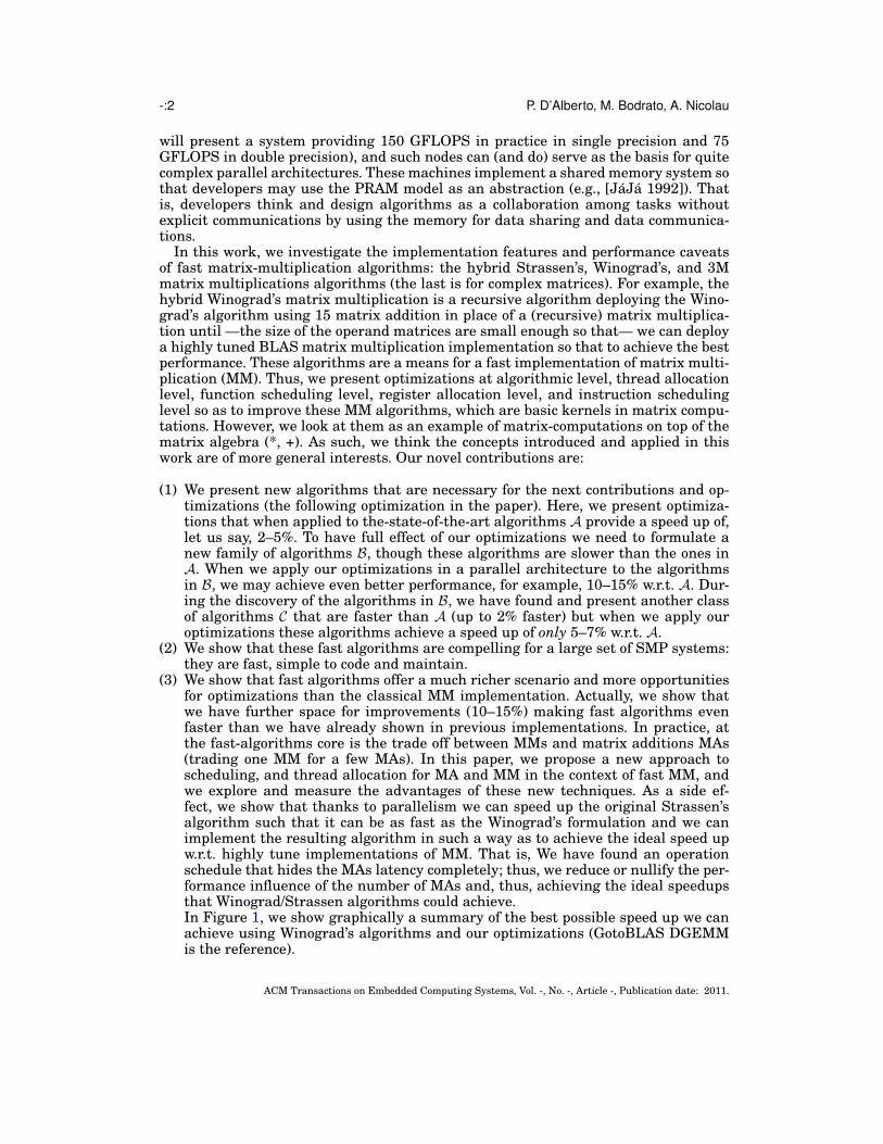
Fig. 2. 4-core 2 Xeon processor: Complex (top) GotoBLAS ZGEMM 14 GFLOPS, ZGEMM 3M 18 GFLOPSand our 3M WINOGRAD 20 GFLOPS; and double precision (bottom) GotoBLAS DGEMM 56 GFLOPS andWINOGRAD 62 GFLOPS. Function pipelining does not provide significant improvements



6.2. AbbreviationsIn the following sections and figures, we use a consistent but not truly standardizedconventions in calling algorithms, we hope this will not be a major problem and thissection should be used whenever consulting a performance plot.

— STRASSEN: Strassen’s algorithms as in Table IV.— WINOGRAD: Winograd’s algorithm as in Table III.— WOPT: Winograd’s algorithm as in Table V with fewer MAs.— WIDEAL: Winograd’s algorithm as in Table VII optimized for a pipeline execution

(but not pipelined).— GOTOS: MM implementation as available in GotoBLAS.— BLAS MM or MM only: MM implementation row-by-column (this is used in the

error analysis only).— (STRASSEN|WINOGRAD|WOPT|WIDEAL) PIPE: software pipeline implemen-

tation of Strassen–Winograd algorithms as in Table IV, III, and VII where someMMs and MAs are interleaved.

— GOTOS 3M: 3M algorithm as available in GotoBLAS where matrices are stored ascomplex matrices.

— 3M (GOTOS|WINOGRAD|STRASSEN|ATLAS): our implementation of the 3Malgorithm as presented in Table II, where MM is implemented as STRASSEN,WINOGRAD, GOTOS, or ATLAS and thus complex matrices are stored as two dis-tinct real matrices.

— 3M (WINOGRAD|STRASSEN) PIPE: our implementation of the 3M algorithmas presented in Table II, where MM is implemented as STRASSEN PIPE, WINO-GRAD PIPE and thus there is software pipelining between MMs and MAs, and com-plex matrices are stored as two real matrices.

6.3. Double-Precision and Complex MatricesWe divide this section into two parts: where software pipelining does not provide anyimprovement (actually is detrimental and not shown) and where software pipeliningprovides performance improvement. Notice that we postpone the experimental resultsfor the optimized Winograd’s algorithm as presented in Section 4.4 in the followingexperiment section (Section 6.3.1), where we present an in depth analysis.

No Software Pipelining. In Figure 2, we show the performance for at least onearchitecture where software pipelining does not work. Notice that the recursion pointis quite large: N=7500 in Figure 2, with a small speed up (up to 2–10%) for doubleprecision matrices. The performance improvements are more effective for complex ma-trices: smaller recursion point (i.e., we can apply fast algorithm for smaller problems)and best speed up (i.e., faster).

Software Pipelining. In Figures 3–5, we present the performance plots for threearchitectures where software pipelining offers performance improvements, we will givemore details in Section 6.3.1.

For only one architecture, 2-core 2 Xeon (Pentium based) Figure 3, the 3M fast al-gorithms have a speedup of 4/3 (+25%) achieving a clean and consistent performanceimprovement. For this architecture, Goto’s MM has best performance when using onlytwo threads (instead of four), and thus this system is underutilized. Using fast algo-rithms and our scheduling optimizations we improve performance consistently.

For the Shanghai system, Figure 4, Goto’s MM achieves peak performance usingall cores, so this architecture is fully utilized. Nonetheless, fast algorithms and opti-mizing schedules achieve a consistent performance improvement. Software pipelining



2.2

2.4

2.6

2.8

3

3.2

3.4

3.6

3.8

1500

1800

2000

2200

2500

2800

3000

3200

3500

3800

4000

4200

4500

4800

5000

5000

5200

5400

5600

5800

6000

6500

7000

7500

8000


3M_WINOGRAD_PIPE

3M_WINOGRAD

3M_STRASSEN_PIPE

WINOGRAD_PIPE

3M_GOTOS

STRASSEN_PIPE

GOTOS_3M

GOTOS

Fig. 3. 2-core 2 Xeon processor (Pentium based): Complex double precision with peak performance Goto-BLAS GEMM 2.4 GFLOPS, GEMM 3M 2.8 GFLOPS, and our 3M WINOGRAD PIPE 3.8 GFLOPS

15

16

17

18

19

20

21

22

23

24

3400

4000

4400

4800

5000

5400

5800

6000

6500

7000

7500

8000

8500

9000

9500

10000

10500

11000

11500

12000


3M_WINOGRAD_PIPE3M_WINOGRAD3M_GOTOSWINOGRAD_PIPEWINOGRADGOTO_3MGOTOS

Fig. 4. 4-core 2 Opteron processor (Shanghai): Complex double precision with GotoBLAS peak per-formance ZGEMM 17 GFLOPS, ZGEMM 3M 20 GFLOPS, and our WINOGRAD 19 GFLOPS and3M WINOGRAD PIPE 23 GFLOPS



16.5

17.5

18.5

19.5

20.5

2501 3001 3501 4001 4501 5001 5401 5801 6501 7501

Normalize2N^3GFLOPS

IDEAL_PIPE

WOPT_PIPE

WINOGRAD_PIPE

WOPT

WINOGRAD

WIDEAL

GOTOS

Fig. 5. 8-core 2 Xeon processor (Nehalem): Complex double precision with GotoBLAS peak performanceZGEMM 17 GFLOPS, our WINOGRAD 19 GFLOPS and WIDEAL PIPE 20.5 GFLOPS

exploits the good bandwidth of the system and, even though MAs are competing forthe resources against the MM, the overhead is very limited.

For the Nehalem system, Figure 5, we have very good speed ups (see the followingsection). This architecture has 4 physical cores for each processor and the architectureis designed to provide task parallelism; each physical core can execute in parallel 2threads for a total of 8 virtual cores providing task as well as thread parallelism; thisis the number of cores the operating system believes exist. Such architecture providesthe best performance overall, just shy of 70 GFLOPS in Double precision, but also thebest scenario for our optimizations.

6.3.1. Double precision: Software Pipelining and Optimized Algorithm. In the previous section,we presented the performance for the MM base line (e.g., GotoBLAS), Winograd, andStrassen with and without function software pipelining. In this section we focus onthe optimized Winograd algorithms (Section 4.4) and the effect of (function) softwarepipelining (with respect to the Winograd’s algorithm without software pipelining). Thiscomparison will highlights the performance advantages of our pipelining optimizations(achieving ideal speedup w.r.t. the GEMM because the MA have not weight nor contri-bution).

We consider three architectures: 2-core 2 Xeon (Pentium Based), 8-core 2 Xeon (Ne-halem), and 2-core 2 Opteron 270 (x86 64). The former two architectures are friendlierto software pipelining than the latter one. The first two architectures are underutilizedbecause we can achieve the best performance with, respectively, two cores and 8 vir-tual cores idle. The latter architecture should provide a smaller space for improvement(if any) because there is no idle core. All architecture will provide information aboutthe algorithms, the optimizations, and the overall performance.

We present odd problem sizes (e.g.,N = 2001, 3001 etc.) because the optimized WOPTalgorithm has potentially fewer MAs and smaller subproblems. We want to quantifysuch a performance advantage. In this section, we present experimental results fordouble (Figure 6–7), and double complex matrices (Figure 9–10). Especially, we presentthe performance advantage of the WIDEAL algorithm (the algorithm that has no MAin the critical path).



‐1

0

1

2

3

4

5

6

7

2601 3001 3501 4001 5001 6001 7001 7501 8001

%speedupvsWINOGRAD WIDEAL_PIPE

WOPT_PIPE

WINOGRAD_PIPE

WOPT

WIDEAL

Fig. 6. 2-core 2 Xeon processor (Pentium Based) double precision: peak speedup WIDEAL PIPE 7% w.r.t.WINOGRAD

‐2

‐1

0

1

2

3

4

5

3501 4001 5001 6001 7001 7501 8001


WOPT_PIPE

WINOGRAD_PIPE

WOPT

WIDEAL

Fig. 7. 2-core 2 Opteron (x86 64) double precision relative: peak speedup WIDEAL PIPE 4% w.r.t. WINO-GRAD

For double precision and for the WIDEAL PIPE algorithm (Figure 6, 7, and 8), weachieve 6% speed up for the Pentium based system, we achieve 4% for the Opteronsystem, and we achieve 10% for the Nehalem system.

For double complex matrices (Figure 9, 10, and 11), we have better relative improve-ments: we achieve 11% speed up for the Pentium based system, 7% for the Opteron,and 12% for the Nehalem (15% if we can perform 3 recursion levels). We show thatWOPT (winograd’s with fewer MAs) has a performance advantage (for these architec-tures) mostly because of the compounding effects of saving operations.

It is clear from the performance plots, that the WIDEAL algorithm has aperformance advantage only when combined with our scheduling optimizations(WIDEAL PIPE), otherwise WIDEAL is always slower than any other algorithms.

Notice that the experimental results for the Nehalem architecture follows the ex-pected seesaw performance as the problem size increases and the recursion number



‐2

0

2

4

6

8

10

12

2501 3001 3501 4001 4501 5001 5401 5801 6501 7501 8501

%speedupvsWINOGRAD

WIDEAL_PIPE

WOPT_PIPE

WINOGRAD_PIPE

WOPT

WIDEAL

Fig. 8. 8-core 2 Xeon (Nehalem) double precision: peak speedup WIDEAL PIPE 11% w.r.t. WINOGRAD

‐1

1

3

5

7

9

11

1601 2001 2601 3001 3501 4001 5001 6001 6501

%speedupvsWINOGRAD

WIDEAL_PIPE

WOPT_PIPE

WINOGRAD_PIPE

WOPT

WIDEAL

Fig. 9. 2-core 2 Xeon processor (Pentium Based) double complex precision: peak speedup WIDEAL PIPE11% w.r.t. WINOGRAD

increases, which follows roughly the formula 2r−1γ/N (where N is the problem sizeand r is the number of recursions (i.e., see Section 4.5 Equation 8).

We know that for the Opteron-based system, there is not idle core and thus our ap-proach will allocate two or more threads onto a single core. Using Goto’s GEMM, weare achieving close to 95% utilization of the cores and thus there should be a very littlespace for improvements. In practice, hiding MAs provides little performance advan-tage for the WINOGRAD and WOP algorithm, however, there is quite a speed up incombination with WIDEAL (i.e., 5–7%).

6.4. Error analysisIn this section, we want to gather the error analysis for a few algorithms (i.e., fast algo-rithms), with different low-level optimizations and hardware operations, using eitherATLAS or GotoBLAS, for single complex and double complex matrices, and for matri-ces in the range |a| ∈ [0, 1] (probability matrices) and |a| ∈ [−1, 1] (scaled matrices).What we present in the following figures can be summarized by a matrix norm:

‖Calg − CDCS‖∞ = max |calgi,j − cDCSi,j |. (9)



‐2

‐1

0

1

2

3

4

5

6

7

8

1601 2001 2601 3001 3501 4001 5001 6001 6501


WOPT_PIPE

WINOGRAD_PIPE

WOPT

WIDEAL

Fig. 10. 2-core 2 Opteron double complex precision relative: peak speedup WIDEAL PIPE 8% w.r.t. WINO-GRAD

‐2

0

2

4

6

8

10

12

2501 3001 3501 4001 4501 5001 5401 5801 6501 7501

%speedupvsWINOGRAD

WIDEAL_PIPE

WOPT_PIPE

WINOGRAD_PIPE

WOPT

WIDEAL

Fig. 11. 8-core 2 Xeon (Nehalem) double complex precision: peak speedup WIDEAL PIPE 12% w.r.t. WINO-GRAD

That is, we present the maximum absolute error. We investigate the error for complexmatrices —thus we can compare all algorithms at once— but instead of showing theabsolute maximum error for the complex matrix we present the maximum error forthe real and imaginary parts of the matrices:

(‖Re(Calg)−Re(CDCS)‖∞, ‖Im(Calg)− Im(CDCS)‖∞

)(10)

We will show that, in practice and for these architectures, the Winograd’s basedalgorithms have similar error than the 3M algorithms and comparable to the BLASclassic algorithm. Furthermore we investigate the effect of the different schedules forthe Winograd’s-based algorithms. Notice, pipeline optimizations do not effect the errorbecause we do not change the order of the computation.

We present a large volume of data, see Figure 12 and and 13.Why two libraries have different error. GotoBLAS and ATLAS have different

way to tailor the code to an architecture. This will provide different tiling techniques.



0.00E+00

2.00E‐13

4.00E‐13

6.00E‐13

8.00E‐13

1.00E‐12

1.20E‐12

1701 2501 3003 3501 4001 4501

maxerror DoubleComplexusingGotoBLAS[‐1,1]Nehalem

ZBLASI‐Z_DCSI

ZBLASR‐Z_DCSR

ZWOPTR‐Z_DCSR

ZWOPTI‐Z_DCSI

Z_3MWinogradR‐Z_DCSR

Z_3MWinogradI‐Z_DCSI

Z_3MGOTOSI‐Z_DCSI

Z_3MGOTOSR‐Z_DCSR

0.00E+00

5.00E‐13

1.00E‐12

1.50E‐12

2.00E‐12

2.50E‐12

3.00E‐12

3.50E‐12

1701 2501 3003 3501 4001 4501

maxerror DoubleComplexusingATLAS[‐1,1]Nehalem

ZWOPTR‐Z_DCSR

ZWOPTI‐Z_DCSI



ZBLASR‐Z_DCSR

ZBLASI‐Z_DCSI

Z_3MATLASR‐Z_DCSR

Z_3MATLASI‐Z_DCSI

Fig. 12. 8-core 2 Xeon Nehalem Error Analysis [-1,1] with respect to the DCS algorithm: (top) based onGotoBLAS and (bottom) based on ATLAS. The GotoBLAS based implementation is 3 times more accuratethan ATLAS based implementation. The GotoBLAS based WOPT (and thus WIDEAL) implementation hasthe same accuracy as the row-by-column definition BLAS implementation. Our 3M implementation has thesame accuracy of GotoBLAS GEMM 3M.

For example, GotoBLAS exhibits a better accuracy (probably because the tiling size islarger). 3

3We reached such a conclusion by our personal communications with the GotoBLAS’ authors and, intuitively,because a larger tile may provide a better register reuse, thus the computation will exploit the internalextended precision of the register file, 90bits, instead of normal encoding in memory using 64bits; that is,inherently a better precision that will fit what we observed and it is against the intuitive idea that a largertile will provide a longer string of additions thus a larger error.



‐1.00E‐12

1.00E‐12

3.00E‐12

5.00E‐12

7.00E‐12

9.00E‐12

1.10E‐11

1.30E‐11

1.50E‐11

1701 2501 3003 3501 4001 4501

maxerror DoubleComplexusingGotoBLAS[0,1]Nehalem

ZBLASI‐Z_DCSI

ZWOPTI‐Z_DCSI

ZWOPTR‐Z_DCSR


Z_3MGOTOSI‐Z_DCSI


Z_3MGOTOSR‐Z_DCSR

ZBLASR‐Z_DCSR

0.00E+00

1.00E‐11

2.00E‐11

3.00E‐11

4.00E‐11

5.00E‐11

6.00E‐11

7.00E‐11

1701 2501 3003 3501 4001 4501

maxerror DoubleComplexusingATLAS[0,1]Nehalem


ZWOPTI‐Z_DCSI


ZBLASI‐Z_DCSI

Z_3MATLASI‐Z_DCSI

Z_3MATLASR‐Z_DCSR

ZWOPTR‐Z_DCSR

ZBLASR‐Z_DCSR

Fig. 13. 8-core 2 Xeon Nehalem Error Analysis [0,1] with respect to the DCS algorithm: (top) based onGotoBLAS and (bottom) based on ATLAS

We want to show that the relative errors (between fast and standard algorithm) areconsistent across BLAS library installations. We show that a better accuracy of thekernels (GotoBLAS GEMMs) will allow a better accuracy of the fast algorithms assignificant as a factor of 3 (1/3 of a digit).

Why comparing real and imaginary parts. We show that the error is differentfor the real and the imaginary part of the computation for several algorithms. In partic-ular, we show that the 3M algorithm tends to have larger error on the imaginary partthan the real part (which is known in the literature). However, we may notice thatthe 3M-Winograd variant has the same error as the BLAS GEMM (row-by-column)computation (and it is two order of magnitude faster than the BLAS GEMM). So the



application of the Winograd algorithm, alone or in combination with the 3M algorithm,has a reasonable error and it should not be discarded a priori.

Why different matrix element ranges. First, the sign of the matrix element af-fects the precision of any operation (cancellation of similar numbers) and the accuracyof the algorithm. It is known in the literature that Winograd’s algorithm is in generalstable for probability matrices (|a| ∈ [0, 1]). We show that variation of the Winograd’salgorithm such as the one with fewer additions may actually loose accuracy with littleperformance advantage. The range of the matrix is chosen such that all the error up-per bounds can be expressed as a polynomial of the matrix size (and there is no needof norm measure).

We present our findings in Figure 12–13. We believe, this is the first attempt to showhow in practice all these algorithms work and how they affect the final result anderror. We do not justify the blind use of fast algorithms when accuracy is paramount;however, we want to make sure that fast algorithms are not rejected just because of anunfounded fear of their instability.

In practice, it’s prohibitively expensive to provide statistics based on DCS algorithm(described in Section 5.1): to gather the experimental results presented in Figure 12–13 took about 2 weeks. To collect, say ten points, it will take about 20 weeks. First, itis not really necessary. Second, if we take a weaker reference (i.e., an algorithm withbetter accuracy because it uses better precision arithmetic double precision instead ofsingle precision), then we may estimate the statistics of the average error and showthat there is no contradictions (with the result presented in the paper Figure 12–13)and in the literature.

Error w.r.t. DGEMM input [0,1]

SGEMM

Fre

quen

cy

0.00074 0.00078 0.00082 0.00086

05

1020

30


S_Winograd

Fre

quen

cy

0.00090 0.00100 0.00110 0.00120

010

2030

4050

60


S_Strassen

Fre

quen

cy

0.0038 0.0042 0.0046

05

1015

2025

30


S_Winograd_Optimal

Fre

quen

cy

0.0030 0.0034 0.0038

05

1020

30

Fig. 14. 2-core 2 Opteron, problem size N=6500, absolute error statistics w.r.t. DGEMM for matrices withinput [0,1]: distribution of the maximum error for GEMM, WINOGRAD, STRASSEN, and WOPT/WIDEALin single precision w.r.t. DGEMM by 100 runs. WINOGRAD is 3 times more accurate on average that WOPTand 0.3 times less accurate than SGEMM



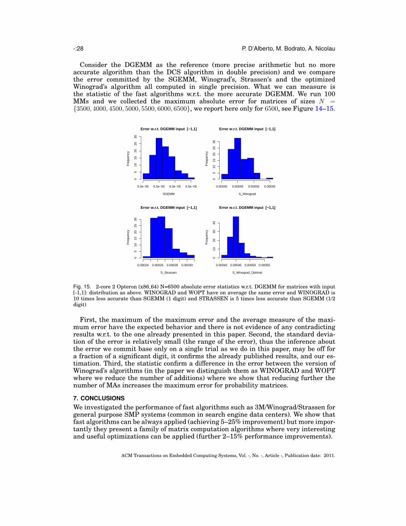
Consider the DGEMM as the reference (more precise arithmetic but no moreaccurate algorithm than the DCS algorithm in double precision) and we comparethe error committed by the SGEMM, Winograd’s, Strassen’s and the optimizedWinograd’s algorithm all computed in single precision. What we can measure isthe statistic of the fast algorithms w.r.t. the more accurate DGEMM. We run 100MMs and we collected the maximum absolute error for matrices of sizes N ={3500, 4000, 4500, 5000, 5500, 6000, 6500}, we report here only for 6500, see Figure 14–15.

Error w.r.t. DGEMM input [−1,1]

SGEMM

Fre

quen

cy

5.0e−05 5.5e−05 6.0e−05 6.5e−05

05

1015

2025

30


S_Winograd

Fre

quen

cy

0.00040 0.00045 0.00050 0.00055

05

1015

2025

30


S_Strassen

Fre

quen

cy

0.00024 0.00026 0.00028 0.00030

05

1015

2025

30


S_Winograd_Optimal

Fre

quen

cy

0.00040 0.00045 0.00050 0.00055

010

2030

40

Fig. 15. 2-core 2 Opteron (x86 64) N=6500 absolute error statistics w.r.t. DGEMM for matrices with input[-1,1]: distribution as above. WINOGRAD and WOPT have on average the same error and WINOGRAD is10 times less accurate than SGEMM (1 digit) and STRASSEN is 5 times less accurate than SGEMM (1/2digit)

First, the maximum of the maximum error and the average measure of the maxi-mum error have the expected behavior and there is not evidence of any contradictingresults w.r.t. to the one already presented in this paper. Second, the standard devia-tion of the error is relatively small (the range of the error), thus the inference aboutthe error we commit base only on a single trial as we do in this paper, may be off fora fraction of a significant digit, it confirms the already published results, and our es-timation. Third, the statistic confirm a difference in the error between the version ofWinograd’s algorithms (in the paper we distinguish them as WINOGRAD and WOPTwhere we reduce the number of additions) where we show that reducing further thenumber of MAs increases the maximum error for probability matrices.

7. CONCLUSIONSWe investigated the performance of fast algorithms such as 3M/Winograd/Strassen forgeneral purpose SMP systems (common in search engine data centers). We show thatfast algorithms can be always applied (achieving 5–25% improvement) but more impor-tantly they present a family of matrix computation algorithms where very interestingand useful optimizations can be applied (further 2–15% performance improvements).



On one side, there is no dominant algorithm for all architectures and all problemsizes. This performance variety should not undermine our overall message: fast al-gorithms can be used in combination with classic MM algorithms and all will thrivewhen used together. On the other side, a few researchers may see the same variety asdiscouraging because there is no clear dominant algorithm: it would be easier to relyon a single common solution.

Here we have shown, that our algorithms and optimizations are simple to applyand they extend the performance of the fastest BLAS libraries for the state of the artarchitectures.

Acknowledgments.The first authors would like to thank Yahoo! to provide the opportunity, to give

the time, and to provide the machines for these experiments. In particular, an heart-felt thank goes to Ali Dasdan, Kelving Fong, Jeff Harlam, Joel Carceres, Greg Ulrichand Arun Kejawal (Yahoo!), Kazushige Goto (Microsoft) and Robert van de Geijn (UTAustin), Clint Whaley (UT San Antonio), and David Wise (Indiana University).

REFERENCESANDERSON, E., BAI, Z., BISCHOF, C., DONGARRA, J. D. J., DUCROZ, J., GREENBAUM, A., HAMMARLING,

S., MCKENNEY, A., OSTROUCHOV, S., AND SORENSEN, D. 1995. LAPACK User’ Guide, Release 2.0 2Ed. SIAM.

BILMES, J., ASANOVIC, K., CHIN, C., AND DEMMEL, J. 1997. Optimizing matrix multiply using PHiPAC:a portable, high-performance, Ansi C coding methodology. In International Conference on Supercomput-ing.

BLACKFORD, L. S., DEMMEL, J., DONGARRA, J., DUFF, I., HAMMARLING, S., HENRY, G., HEROUX, M.,KAUFMAN, L., LUMSDAINE, A., PETITET, A., POZO, R., REMINGTON, K., AND WHALEY, R. C. 2002.An updated set of basic linear algebra subprograms (BLAS). ACM Transaction in Mathemathical Soft-ware 28, 2, 135–151.

BODRATO, M. 2010. A Strassen-like matrix multiplication suited for squaring and higher power computa-tion. In ISSAC ’10: Proceedings of the 2010 international symposium on Symbolic and algebraic compu-tation. ACM, New York, NY, USA. http://bodrato.it/papers/#ISSAC2010.

BOYER, B., DUMAS, J.-G., PERNET, C., AND ZHOU, W. 2009. Memory efficient scheduling of Strassen-Winograd’s matrix multiplication algorithm. In ISSAC. 55–62.

BRENT, R. P. 1970a. Algorithms for matrix multiplication. Tech. Rep. TR-CS-70-157, Stanford University.Mar.

BRENT, R. P. 1970b. Error analysis of algorithms for matrix multiplication and triangular decompositionusing Winograd’s identity. Numerische Mathematik 16, 145–156.

COHN, H., KLEINBERG, R., SZEGEDY, B., AND UMANS, C. 2005. Group-theoretic algorithms for matrixmultiplication.

COPPERSMITH, D. AND WINOGRAD, S. 1987. Matrix multiplication via arithmetic progressions. In Proceed-ings of the 19-th annual ACM conference on Theory of computing. 1–6.

D’ALBERTO, P. AND NICOLAU, A. 2007. Adaptive strassen’s matrix multiplication. In ICS ’07: Proceedingsof the 21st annual international conference on Supercomputing. ACM, New York, NY, USA, 284–292.

D’ALBERTO, P. AND NICOLAU, A. 2009. Adaptive Winograd’s matrix multiplications. ACM Transactions onMathematical Software 36, 1.

DEMMEL, J., DONGARRA, J., EIJKHOUT, E., FUENTES, E., PETITET, E., VUDUC, V., WHALEY, R., ANDYELICK, K. 2005. Self-Adapting linear algebra algorithms and software. Proceedings of the IEEE, spe-cial issue on ”Program Generation, Optimization, and Adaptation” 93, 2.

DEMMEL, J., DUMITRIU, J., HOLTZ, O., AND KLEINBERG, R. 2006. Fast matrix multiplication is stable.DEMMEL, J. AND HIGHAM, N. 1992. Stability of block algorithms with fast level-3 BLAS. ACM Transactions

on Mathematical Software 18, 3, 274–291.DONGARRA, J. J., CROZ, J. D., DUFF, I. S., , AND HAMMARLING, S. 1990a. Algorithm 679: A set of level 3

Basic Linear Algebra Subprograms. ACM Transaction in Mathemathical Software 16, 18–28.DONGARRA, J. J., CROZ, J. D., DUFF, I. S., , AND HAMMARLING, S. 1990b. A set of level 3 Basic Linear

Algebra Subprograms. ACM Transaction in Mathemathical Software 16, 1–17.


http://bodrato.it/papers/#ISSAC2010


DOUGLAS, C., HEROUX, M., SLISHMAN, G., AND SMITH, R. 1994. GEMMW: A portable level 3 BLAS Wino-grad variant of Strassen’s matrix–matrix multiply algorithm. J. Comp. Phys. 110, 1–10.

DUMAS, J.-G., GIORGI, P., AND PERNET, C. 2008. Dense linear algebra over word-size prime fields: theFFLAS and FFPACK packages. ACM Trans. Math. Softw. 35, 3, 1–42.

EIRON, N., RODEH, M., AND STEINWARTS, I. 1998. Matrix multiplication: a case study of algorithm engi-neering. In Proceedings WAE’98. Saarbrucken, Germany.

FRENS, J. AND WISE, D. 1997. Auto-Blocking matrix-multiplication or tracking BLAS3 performance fromsource code. Proc. 1997 ACM Symp. on Principles and Practice of Parallel Programming 32, 7, 206–216.

FRIGO, M. AND JOHNSON, S. 2005. The design and implementation of FFTW3. Proceedings of the IEEE,special issue on ”Program Generation, Optimization, and Adaptation” 93, 2, 216–231.

GOTO, K. AND VAN DE GEIJN, R. 2008. Anatomy of high-performance matrix multiplication. ACM Trans-actions on Mathematical Software.

GUNNELS, J., GUSTAVSON, F., HENRY, G., AND VAN DE GEIJN, R. 2001. FLAME: Formal Linear AlgebraMethods Environment. ACM Transactions on Mathematical Software 27, 4, 422–455.

HIGHAM, N. 1990. Exploiting fast matrix multiplication within the level 3 BLAS. ACM Trans. Math.Softw. 16, 4, 352–368.

HIGHAM, N. 2002. Accuracy and Stability of Numerical Algorithms, Second Edition. SIAM.HUSS-LEDERMAN, S., JACOBSON, E., JOHNSON, J., TSAO, A., AND TURNBULL, T. 1996. Strassen’s al-

gorithm for matrix multiplication: Modeling analysis, and implementation. Tech. Rep. CCS-TR-96-14,Center for Computing Sciences.

HUSS-LEDERMAN, S., JACOBSON, E., TSAO, A., TURNBULL, T., AND JOHNSON, J. 1996. Implementa-tion of Strassen’s algorithm for matrix multiplication. In Supercomputing ’96: Proceedings of the 1996ACM/IEEE conference on Supercomputing (CDROM). ACM Press, 32.

JAJA, J. 1992. An introduction to parallel algorithms. Addison Wesley Longman Publishing Co., Inc., Red-wood City, CA, USA.

KAGSTROM, B., LING, P., AND VAN LOAN, C. 1998a. Algorithm 784: GEMM-based level 3 BLAS: portabilityand optimization issues. ACM Transactions on Mathematical Software 24, 3, 303–316.

KAGSTROM, B., LING, P., AND VAN LOAN, C. 1998b. GEMM-based level 3 BLAS: high-performance modelimplementations and performance evaluation benchmark. ACM Transactions on Mathematical Soft-ware 24, 3, 268–302.

KAPORIN, I. 1999. A practical algorithm for faster matrix multiplication. Numerical Linear Algebra withApplications 6, 8, 687–700. Centre for Supercomputer and Massively Parallel Applications, ComputingCentre of the Russian Academy of Sciences, Vavilova 40, Moscow 117967, Russia.

KAPORIN, I. 2004. The aggregation and cancellation techniques as a practical tool for faster matrix multi-plication. Theor. Comput. Sci. 315, 2-3, 469–510.

LAWSON, C. L., HANSON, R. J., KINCAID, D., AND KROGH, F. T. 1979. Basic Linear Algebra Subprogramsfor FORTRAN usage. ACM Transaction in Mathemathical Software 5, 308–323.

LOOS, S. AND WISE, D. Strassen’s matrix multiplication relabeled.NICOLAU, A., LI, G., AND KEJARIWAL, A. 2009. Techniques for efficient placement of synchronization prim-

itives. In PPoPP ’09: 14th ACM SIGPLAN Symposium on Principles and Practice of Parallel Program-ming.

PAN, V. 1978. Strassen’s algorithm is not optimal: Trililnear technique of aggregating, uniting and cancelingfor constructing fast algorithms for matrix operations. In FOCS. 166–176.

PAN, V. 1984. How can we speed up matrix multiplication? SIAM Review 26, 3, 393–415.PRIEST, D. 1991. Algorithms for arbitrary precision floating point arithmetic. In Proceedings of the 10th

IEEE Symposium on Computer Arithmetic (Arith-10), P. Kornerup and D. W. Matula, Eds. IEEE Com-puter Society Press, Los Alamitos, CA, Grenoble, France, 132–144.

PUSCHEL, M., MOURA, J., JOHNSON, J., PADUA, D., VELOSO, M., SINGER, B., XIONG, J., FRANCHETTI,F., GACIC, A., VORONENKO, Y., CHEN, K., JOHNSON, R., AND RIZZOLO, N. 2005. SPIRAL: Code gener-ation for DSP transforms. Proceedings of the IEEE, special issue on ”Program Generation, Optimization,and Adaptation” 93, 2.

STRASSEN, V. 1969. Gaussian elimination is not optimal. Numerische Mathematik 14, 3, 354–356.WHALEY, R. AND DONGARRA, J. 1998. Automatically tuned linear algebra software. In Proceedings of the

1998 ACM/IEEE conference on Supercomputing (CDROM). IEEE Computer Society, 1–27.WHALEY, R. C. AND PETITET, A. 2005. Minimizing development and maintenance costs in

supporting persistently optimized BLAS. Software: Practice and Experience 35, 2, 101–121.http://www.cs.utsa.edu/~whaley/papers/spercw04.ps.


exploiting parallelism in matrix-computation kernels for ...paolo/reference/dalbertobn2011.pdf ·...

Documents