HAL Id: hal-00438190https://hal.archives-ouvertes.fr/hal-00438190v1

Submitted on 2 Dec 2009 (v1), last revised 18 Nov 2010 (v3)

HAL is a multi-disciplinary open accessarchive for the deposit and dissemination of sci-entific research documents, whether they are pub-lished or not. The documents may come fromteaching and research institutions in France orabroad, or from public or private research centers.

L’archive ouverte pluridisciplinaire HAL, estdestinée au dépôt et à la diffusion de documentsscientifiques de niveau recherche, publiés ou non,émanant des établissements d’enseignement et derecherche français ou étrangers, des laboratoirespublics ou privés.

Explicit expression of the counting generating functionfor Gessel’s walk

Irina Kurkova, Kilian Raschel

To cite this version:Irina Kurkova, Kilian Raschel. Explicit expression of the counting generating function for Gessel’swalk. 20 pages, 4 figures. 2009. <hal-00438190v1>

Explicit expression of the counting

generating function for Gessel’s walk

Irina Kurkova∗ Kilian Raschel∗

December 2, 2009

Abstract

We consider the so-called Gessel’s walk, that is the planar random walk that isconfined to the first quadrant and that can move in unit steps to the West, North-East,East and South-West. For this walk we make explicit the generating function of thenumber of paths starting at (0, 0) and ending at (i, j) in time k.

Keywords : lattice walks, generating function, Riemann-Hilbert boundary value problem,conformal gluing function, Weierstrass elliptic function, Riemann surface, uniformization.

AMS 2000 Subject Classification : primary 05A15 ; secondary 30F10, 30D05.

0 Introduction and main results

The enumeration of lattice walks is a classical problem in combinatorics. The one ofGessel’s walk seems to puzzle the mathematics community already for several years[Ges86, PW08, KKZ09, Ayy09, Pin09, BK09]. This is a planar random walk that isconfined to the first quadrant and that can move in the interior in unit steps to the West,North-East, East and South-West, see Figure 1. For (i, j) ∈ Z

2+ and k ∈ Z+, set

q(i, j, k) = #walks starting at (0, 0) and ending at (i, j) in time k

.

I. Gessel conjectured around 2001 that q(2k, 0, 0) = 16k[(5/6)k(1/2)k

]/[(2)k(5/3)k

], where

(a)k = a(a+1) · · · (a+k−1). In 2008, M. Kauers, C. Koutschan and D. Zeilberger yieldeda remarkable although heavily computer-aided proof of this conjecture, see [KKZ09].

The articles [Ayy09, Pin09] give connections between Gessel’s walk and otherinteresting models. Namely, S. Ping in [Pin09] establishes a probabilistic model for Gessel’s

∗Laboratoire de Probabilites et Modeles Aleatoires, Universite Pierre et Marie Curie, 4 Place Jussieu75252 Paris Cedex 05, France. E-mails : irina.kourkova@upmc.fr, kilian.raschel@upmc.fr.

1

walk concerned with vicious walkers, and A. Ayyer in [Ayy09] interprets such walks asDick words with two sets of letters and gives explicit formulas for a restricted class ofsuch words. Both of these approaches are yet in some way of providing “human” proof ofGessel conjecture but may certainly help for a better understanding of Gessel’s walk.

M. Petkovsek and H. Wilf in [PW08] state some similar conjectures for the numberof walks ending at other points. Two of them have been proved by S. Ping in [Pin09].M. Petkovsek and H. Wilf in [PW08] obtain also an infinite lower-triangular system oflinear equations satisfied by the values of f(k, i, 0) and f(k, 0, j)+f(k, 0, j−1) and expressthese values as determinants of lower-Hessenberg matrices with unit superdiagonals whosenon-zero entries are products of two binomial coefficients.

Finally, A. Bostan and M. Kauers in [BK09] show that the complete generating functionfor Gessel’s walk

Q(x, y, z) =∑

i,j,k≥0

q(i, j, k)xiyjzk

is algebraic. Their proof involves, among other tools, computer calculations using apowerful computer algebra system Magma, it required immense computational effort.

Curiously, in spite of this vivid interest to Gessel’s walk, the complete generatingfunction Q(x, y, z) or even Q(0, y, z) or Q(x, 0, z) have not been yet make explicit in aclosed form. Furthermore, recently M. Bousquet-Melou and M. Mishna have undertakenthe systematic analysis of enumeration of the walks confined to the quarter plane Z

2+

starting from the origin and making steps at any point of Z2+ from a given subset of

−1, 0, 12\(0, 0). There are 28 such models. Moreover they show that, after eliminatingtrivial models and those that are equivalent to models of walks confined to a half-planeand solved by known methods, it remains 79 inherently different problems to study.Following the idea of Book [FIM99], they associate to each model a group G of birationaltransformations (for details on this group, see Subsection 1.1 below). This group is finitein 23 cases and infinite in the 56 other cases. They are able to solve 22 models associatedwith a finite group. The only case with finite group that remained unsolved is the modelof Gessel’s walk.

The aim of this paper is to solve Gessel’s walk model, i.e. to represent in a closed formthe generating function Q(x, y, z).

Let us observe that for any i and j, q(k, i, j) ≤ 4k, so that Q(x, y, z) is holomorphic in|x| < 1, |y| < 1, |z| < 1/4 and continuous up to |x| ≤ 1, |y| ≤ 1, |z| < 1/4. Our startingpoint is the functional equation already stated in [BMM08] and exploited in [PW08], valida priori on |x| ≤ 1, |y| ≤ 1, |z| < 1/4 :

L(x, y, z)Q(x, y, z) = zQ(x, 0, z) + z(y + 1)Q(0, y, z) − zQ(0, 0, z) − xy, (1)

where L(x, y, z) = xyz[1/x + 1/(xy) + x+ xy − 1/z

].

2

Figure 1: Gessel’s walk

Our method heavily relies on the profound analytic approach developed in Book[FIM99] by G. Fayolle, R. Iasnogorodski and V. Malyshev. There the authors computethe generating functions of stationary probabilities for some ergodic random walks in thequarter plane. These random walks have four domains of spatial homogeneity : the interior(i, j) : i > 0, j > 0, the x-axis (i, 0) : i > 0, the y-axis (0, j) : j > 0 and the origin0, 0 ; in the interior the only (at most eight) possible non-zero jump probabilities are atdistance one. They reduce the problem to the solution of the following functional equationon |x| ≤ 1, |y| ≤ 1,

K(x, y)Π(x, y) = k(x, y)π(x) + k(x, y)π(y) + k0(x, y)π00, (2)

with known polynomials K(x, y), k0(x, y), k(x, y), k(x, y) and with functions Π(x, y),π(x), π(y) unknown but holomorphic in unit discs, continuous up to the boundary. First,they continue π(x) and π(y) as meromorphic (with poles that can be identified) to thewhole complex plane cut along some segment. This ingenious continuation procedure isthe crucial step of Book [FIM99]. After that, they show that π(x) and π(y) verify aboundary value problem of Riemann-Carleman type, and they solve it by converting itinto a boundary value problem of Riemann-Hilbert type.

Compared to (2), our equation (1) seems a bit more difficult to analyze, as it involves acomplementary parameter z, that we will suppose to be fixed in ]0, 1/4[, so that zQ(x, 0, z)is an unknown function of x ∈ |x| ≤ 1 and z(y + 1)Q(x, y, z) is an unknown function ofy ∈ |y| ≤ 1. From the other point of view, the coefficients k0(x, y), k(x, y) and k(x, y) infront of unknowns zQ(x, 0, z), z(y+1)Q(0, y, z) and zQ(0, 0, z) are absent. This will allowus to continue zQ(x, 0, z) and z(y+1)Q(0, y, z) as holomorphic and not only meromorphicfunctions and, consequently, to simplify substantially the solution.

We are now going to state the main results of this paper. To begin with, let us havea closer look to the kernel L(x, y, z) that appears in (1) and let us take some notations.

The polynomial L(x, y, z) can be written as L(x, y, z) = a(y, z)x2 + b(y, z)x+ c(y, z) =a(x, z)y2 + b(x, z)y + c(x, z), with a(y, z) = zy(y + 1), b(y, z) = −y, c(y, z) = z(y + 1)

3

and a(x, z) = zx2, b(x, z) = zx2 − x + z, c(x, z) = z. Define also d(y, z) = b(y, z)2 −4a(y, z)c(y, z) and d(x, z) = b(x, z)2 − 4a(x, z)c(x, z).

For any z ∈]0, 1/4[, d has one root equal to zero and two real positive roots, thatwe denote by y2(z) < 1 < y3(z). We have y2(z) = [1 − 8z2 − (1 − 16z2)1/2]/[8z2] andy3(z) = [1 − 8z2 + (1 − 16z2)1/2]/[8z2] ; we will also note y1(z) = 0 and y4(z) = ∞.

Likewise, for all z ∈]0, 1/4[, d has four real positive roots, that we denote by x1(z) <x2(z) < 1 < x3(z) < x4(z). Their explicit expression is x1(z) = [1 + 2z− (1 + 4z)1/2]/[2z],x2(z) = [1 − 2z − (1 − 4z)1/2]/[2z], x3(z) = [1 − 2z + (1 − 4z)1/2]/[2z] and x4(z) =[1 + 2z + (1 + 4z)1/2]/[2z].

With these notations we have L(x, y, z) = 0 if and only if (b(y, z)+2a(y, z)x)2 = d(y, z)or (b(x, z)+2a(x, z)y)2 = d(x, z). In particular, the algebraic functionsX(y, z) and Y (x, z)defined by L(X(y, z), y, z) = 0 and L(x, Y (x, z), z) = 0 have two branches, meromorphicon respectively C \

([y1(z), y2(z)] ∪ [y3(z), y4(z)]

)and C \

([x1(z), x2(z)] ∪ [x3(z), x4(z)]

).

The following straightforward results give some properties of the two branches of thealgebraic functions X(y, z) and Y (x, z).

Lemma 1. Call X0(y, z) = [−b(y, z) + d(y, z)1/2]/[2a(y, z)] and X1(y, z) = [−b(y, z) −d(y, z)1/2]/[2a(y, z)] the branches of X(y, z). For all y ∈ C, we have |X0(y, z)| ≤ |X1(y, z)|.

On C \([y1(z), y2(z)] ∪ [y3(z), y4(z)]

), X0 has a simple zero at −1, no other zero and

no pole ; X1 has a simple pole at −1, no other pole and no zero. Finally, both X0 and X1

become infinite at y1(z) = 0 and zero at y4(z) = ∞.Now we call Y0(x, z) = [−b(x, z) + d(x, z)1/2]/[2a(x, z)] and Y1(x, z) = [−b(x, z) −

d(x, z)1/2]/[2a(x, z)] the branches of Y (x, z). For all x ∈ C, we have |Y0(x, z)| ≤ |Y1(x, z)|.On C \

([x1(z), x2(z)] ∪ [x3(z), x4(z)]

), Y0 has a double zero at ∞, no other zero and

no pole ; Y1 has a double pole at 0, no other pole and no zero.

Both Xi(y, z), i = 0, 1, are not defined for y in a branch cut, in other words fory ∈ [y1(z), y2(z)] ∪ [y3(z), y4(z)]. However, the limits X±

i (y, z) defined by X+i (y, z) =

limXi(y, z) as y → y from the upper side of the cut and X−i (y, z) = limXi(y, z) as y → y

from the lower side of the cut are well defined. Since for y in a branch cut, d(y, z) < 0,these two quantities are complex conjugate the one from the other.

A similar remark holds for Yi(x, z), i = 0, 1, for x ∈ [x1(z), x2(z)] ∪ [x3(z), x4(z)].In fact we have :

X±0 (y, z) =

−b(y, z) ∓ ı[− d(y, z)

]1/2

2a(y, z), Y ±

0 (x, z) =−b(x, z) ∓ ı

[− d(x, z)

]1/2

2a(x, z), (3)

X±1 (y, z) = X∓

0 (y, z) and Y ±1 (x, z) = Y ∓

0 (x, z).

Lemma 2. Consider X([y1(z), y2(z)], z) and Y ([x1(z), x2(z)], z). (i) These two curves aresymmetrical w.r.t. the real axis and not included in the unit disc. (ii) X([y1(z), y2(z)], z)contains ∞, Y ([x1(z), x2(z)], z) is closed. (iii) Both of them split the plane into

4

two connected components, we call GX([y1(z), y2(z)], z) and GY ([x1(z), x2(z)], z) theconnected components of 0. They verify GX([y1(z), y2(z)], z) ⊂ C \ [x3(z), x4(z)] andGY ([x1(z), x2(z)], z) ⊂ C \ [y3(z), y4(z)].

31 (z) 2x (z) y2 (z)(z)y1

(z)y1 y2 (z) x1 (z) 2x (z)

3 4x x(z) (z) (z)(z)x3

],z)X([ , Y([ , ],z)

yx

Figure 2: The curves X([y1(z), y2(z)], z) and Y ([x1(z), x2(z)], z)

Note that complete proofs of Lemmas 1 and 2 can be found in Part 5.3 of [FIM99].These notations and results on the kernel L(x, y, z) are enough in order to state our results.

First of all, we would like to show that zQ(x, 0, z) and z(y + 1)Q(0, y, z) verify someboundary value problem of Riemann-Carleman type. It turns out that the associatedboundary conditions verified by zQ(x, 0, z) and z(y+ 1)Q(0, y, z) hold respectively on thecurves X([y1(z), y2(z)], z) and Y ([x1(z), x2(z)], z), which are not included in unit disc,where the functions zQ(x, 0, z) and z(y + 1)Q(0, y, z) are thus a priori not defined. Forthis reason, we first need to continue the generating functions up to these curves. In factwe will prove the following – the proof of which being the central subject of Section 2.

Theorem 3. The functions zQ(x, 0, z) and z(y + 1)Q(0, y, z) can be holomorphicallycontinued from their unit disc up to C \ [x3(z), x4(z)] and C \ [y3(z), y4(z)] respectively.Furthermore for any y ∈ C \ [y1(z), y2(z)] ∪ [y3(z), y4(z)],

zQ(X0(y, z), 0, z) + z(y + 1)Q(0, y, z) − zQ(0, 0, z) −X0(y, z)y = 0, (4)

and for any x ∈ C \ [x1(z), x2(z)] ∪ [x3(z), x4(z)],

zQ(x, 0, z) + z(Y0(x, z) + 1)Q(0, Y0(x, z), z) − zQ(0, 0, z) − xY0(x, z) = 0. (5)

Remark 4. For y ∈ |y| ≤ 1 such that |X0(y, z)| ≤ 1, (4) follows immediately from (1).Likewise, (5) is a straightforward consequence of (1) for any x ∈ |x| ≤ 1 such that|Y0(x, z)| ≤ 1. The fact that equations (4) and (5) are verified not only for these values ofy and x but actually on C\ [y1(z), y2(z)]∪ [y3(z), y4(z)] and C\ [y1(z), y2(z)]∪ [x3(z), x4(z)]respectively will be shown in Section 2.

5

Remark 5. In the proof of Theorem 3, we will see that the function zQ(0, y, z) can alsobe holomorphically continued from the unit disc up to C \ [y3(z), y4(z)].

Now we explain how to obtain the above mentioned boundary conditions verified bythe functions zQ(x, 0, z) and z(y + 1)Q(0, y, z).

Let y ∈ [y1(z), y2(z)], and let y+ and y− be close to y, such that y+ is in the upper half-plane and y− in the lower half-plane. Then we have (4) for both y+ and y−. If now y+ → yand y− → y, then we obtain X0(y

+, z) → X+0 (y, z) and X0(y

−, z) → X−0 (y, z) = X+

1 (y, z).So we have proved that for any y ∈ [y1(z), y2(z)],

zQ(X+0 (y, z), 0, z) + z(y + 1)Q(0, y, z) − zQ(0, 0, z)−X+

0 (y, z)y = 0, (6)

zQ(X+1 (y, z), 0, z) + z(y + 1)Q(0, y, z) − zQ(0, 0, z)−X+

1 (y, z)y = 0. (7)

Substracting (7) from (6) we get that for any y ∈ [y1(z), y2(z)],

z[Q(X+

0 (y, z), 0, z) −Q(X+1 (y, z), 0, z)

]= X+

0 (y, z)y −X+1 (y, z)y. (8)

Then, using the fact that for i = 0, 1, y ∈ [y1(z), y2(z)] and z ∈]0, 1/4[, Y0(X±i (y, z), z) = y

– which can be proved by elemantary considerations starting from Lemma 1, or by theuse of Lemma 17 –, we get the first part of (9) below :

∀t ∈ X([y1(z), y2(z)], z) : z[Q

(t, 0, z

)−Q

(t, 0, z

)]= tY0

(t, z

)−tY0

(t, z

),

∀t ∈ Y ([x1(z), x2(z)], z) : z[(t+ 1

)Q

(0, t, z

)−

(t+ 1

)Q

(0, t, z

)]= X0

(t, z

)t−X0

(t, z

)t.(9)

Likewise, we could prove the second part of (9).Note that as a consequence of (6) and (7), (4) is in some sense also verified for

y ∈ [y1(z), y2(z)] – the same is true for (5) and x ∈ [x1(z), x2(z)].

With Lemma 2, Theorem 3 and (9), we get that zQ(x, 0, z) and z(y+1)Q(0, y, z) can befound among the functions holomorphic in GX([y1(z), y2(z)], z) and GY ([x1(z), x2(z)], z),continuous up to the boundary and verifying the boundary conditions (9).

A such problem is called a boundary value problem of Riemann-Carleman type. Astandard way to solve it consists in converting it to a boundary value problem of Riemann-Hilbert type by use of a conformal gluing function (CGF).

For any detail about boundary value problems and conformal gluing, we refer to [Lit00].

Definition 6. Let C ⊂ C \ 0 be a curve symmetrical w.r.t. the real axis and splittingthe complex plane into two connected components, and let GC be the connected componentof 0. A function u is said to be a CGF for the curve C if (i) u is meromorphic in GC(ii) u establishes a conformal mapping of GC onto the complex plane cut along some arc(iii) for all t ∈ C, u

(t)

= u(t).

Let w(t, z) and w(t, z) be CGF for X([y1(z), y2(z)], z) and Y ([x1(z), x2(z)], z) – theexistence (but no explicit expression) of w and w is ensured by general results on conformalgluing.

6

Transforming the boundary value problems of Riemann-Carleman type into boundaryvalue problems of Riemann-Hilbert type thanks to w and w, solving them and workingout the solutions we will prove the following.

Theorem 7. The function z[Q(x, 0, z) −Q(0, 0, z)

]has the following explicit expression

for z ∈]0, 1/4[ and x ∈ C \ [x3(z), x4(z)] :

z[Q(x, 0, z) −Q(0, 0, z)

]=

xY0(x, z) +1

π

∫ x2(z)

x1(z)

t[− d(t, z)

]1/2

2a(t, z)

[∂tw(t, z)

w(t, z) − w(x, z)−

∂tw(t, z)

w(t, z) −w(0, z)

]dt,

w being a CGF for the curve X([y1(z), y2(z)], z).

The function z[(y + 1)Q(0, y, z) − Q(0, 0, z)

]has the following explicit expression for

z ∈]0, 1/4[ and y ∈ C \ [y3(z), y4(z)] :

z[(y + 1)Q(0, y, z) −Q(0, 0, z)

]=

X0(y, z)y +1

π

∫ y2(z)

y1(z)

t[− d(t, z)

]1/2

2a(t, z)

[∂tw(t, z)

w(t, z) − w(y, z)−

∂tw(t, z)

w(t, z) − w(0, z)

]dt,

w being a CGF for the curve Y ([x1(z), x2(z)], z).

The function Q(0, 0, z) has the following explicit expression for z ∈]0, 1/4[ :

Q(0, 0, z) = −1

π

∫ y2(z)

y1(z)

t[− d(t, z)

]1/2

2a(t, z)

[∂tw(t, z)

w(t, z) − w(−1, z)−

∂tw(t, z)

w(t, z) − w(0, z)

]dt,

w being a CGF for the curve Y ([x1(z), x2(z)], z).

The function Q(x, y, z) has the explicit expression obtained by using the ones ofQ(x, 0, z), Q(0, y, z) and Q(0, 0, z) in (1).

All functions in the integrands above are explicit, except for the CGF w and w.In [FIM99] suitable CGF are computed implicitly by means of the reciprocal of someknown functions (see the formulas (24) and (25) below for the details). Starting from thisrepresentation, we are able to make explicit these functions for Gessel’s walk.

In order to state the result we need to define G2(z) = (4/27)(1 + 224z2 + 256z4),G3(z) = (8/729)(1+16z2)(1−24z+16z2)(1+24z+16z2), K(z) as the only positive root ofK4−G2(z)K

2/2−G3(z)K−G2(z)2/48 = 0 – noting rk(z) = [G2(z)−exp(2kıπ/3)(G2(z)

3−27G3(z)

2)1/3]/3 we have K(z) = [−r0(z)1/2 + r1(z)

1/2 + r2(z)1/2]/2 – and

F (t, z) =1 − 24z + 16z2

3−

4(1 − 4z)2

z

t2

(t− x2(z))(t − 1)2(t− x3(z)),

F (t, z) =1 − 24z + 16z2

3+

4(1 − 4z)2

z

t(t+ 1)2

[(t− x2(z))(t − x3(z))]2.

(10)

7

Theorem 8. A suitable CGF for the curve X([y1(z), y2(z)], z) is the only function havinga pole at x2(z) and solution of

w3 −w2[F (t, z)+ 2K(z)

]+ w

[2K(z)F (t, z) +K(z)2/3 +G2(z)/2

]

−[K(z)2F (t, z) + 19G2(z)K(z)/18 +G3(z) − 46K(z)3/27

]= 0.

(11)Likewise, a suitable CGF for the curve Y ([x1(z), x2(z)], z) is the only function having apole at x3(z) and solution of the equation obtained from (11) by replacing F by F , see (10).

Let us now outline some facts around Theorems 3, 7 and 8.

Remark 9. Since (1) is valid at least on |x| ≤ 1, |y| ≤ 1, |z| < 1/4, then for any such(x, y, z) with L(x, y, z) = 0, the right-hand side of (1) equals zero, so that

z[Q(x, 0, z) −Q(0, 0, z)

]+ z

[(y + 1)Q(0, y, z) −Q(0, 0, z)

]+ zQ(0, 0, z) − xy = 0. (12)

We deduce that

zQ(0, 0, z) = −z[Q(x, 0, z) −Q(0, 0, z)

]− z

[(y + 1)Q(0, y, z) −Q(0, 0, z)

]+ xy. (13)

In Theorem 7 we have chosen to substitute (x, y, z) = (0,−1, z), which is such thatL(x, y, z) = 0 since X0(−1, z) = 0, see Lemma 1. Moreover, we show in Theorem 3 that forany z ∈]0, 1/4[, the equation (12) is valid not only on (x, y) ∈ C

2 : L(x, y, z) = 0∩|x| ≤1, |y| ≤ 1 but in a much larger domain of the algebraic curve (x, y) ∈ C

2 : L(x, y, z) = 0.Namely, if (x, y) is such that x 6∈ [x3(z), x4(z)] and y = Y0(x, z) or y 6∈ [y3(z), y4(z)] andx = X0(y, z), then (12) is still valid. Substituting any (x, y) from this domain into (12)yields us zQ(0, 0, z) as in (13).

Remark 10. With the analytical approach proposed here, it would be possible, withoutadditional difficulty, to obtain explicitly the generating function of the number of walksbeginning at an arbitrary initial state (i0, j0) and ending at (i, j) in time k. Indeed, theonly significant difference is that the product xy in (1) would be then replaced by xi0+1yj0+1.

Remark 11. Making in Theorem 7 the changes of variable w = w(t, z) and w = w(t, z),we obtain that the generating functions zQ(x, 0, z) and z(y + 1)Q(0, y, z) are essentiallyCauchy-type integrals of algebraic functions.

In particular, it could be deduced from the work [PRY04] – which gives criteria for aCauchy-type integral of an algebraic function to be algebraic – that as functions of x andy respectively, zQ(x, 0, z) and z(y + 1)Q(0, y, z) are algebraic functions, what would givean other proof to some results contained in [BK09].

Remark 12. In Theorem 7, the functions z[Q(x, 0, z)−Q(0, 0, z)

]and z

[(y+1)Q(0, y, z)−

Q(0, 0, z)]

are written as the sum of two functions not holomorphic but algebraic nearrespectively [x1(z), x2(z)] and [y1(z), y2(z)]. The sum of these two algebraic functions is

8

of course holomorphic near these segments. By an application of the residue theorem asin Section 4 of [KR09], we could write both generating functions as functions manifestlyholomorphic near these segments and having in fact their first singularity at respectivelyx3(z) and y3(z).

The rest of the paper is organized as follows.In Section 1 we prove Theorem 8. There the implicit representation of the CGF given

in [FIM99] (recalled here in Subsections 1.1 and 1.2) in a general setting is developed inSubsection 1.3 to the case of Gessel’s walk.

The proof of Theorem 3 is postponed to the last Section 2. The main idea of theholomorphic continuation procedure is borrowed again from [FIM99], we show how itworks with the parameter z ∈]0, 1/4[. Finally we give the proof of Theorem 7.

Proof of Theorem 7. The proof is composed of two steps : the first one, inspiredby [FIM99], will allow us to obtain integral representations of the functions zQ(x, 0, z) andz(y+1)Q(0, y, z) on the curves X([y1(z), y2(z)], z) and Y ([x1(z), x2(z)], z) ; the second onewill consist in transforming these formulations into the integrals on real segments writtenin the statement of Theorem 7.

Let us begin by solving the boundary value problems of Riemann-Carleman type withboundary conditions (9). The use of CGF allows us, as in [FIM99] or [Lit00], to transformthem into boundary value problems of Riemann-Hilbert type. Following again [FIM99]or [Lit00] we solve them and in this way we obtain representations of the unknown functionszQ(x, 0, z) and z(y + 1)Q(0, y, z) as integrals along the curves X([y1(z), y2(z)], z) andY ([x1(z), x2(z)], z). For zQ(x, 0, z), we get that up to some additive function of z,

zQ(x, 0, z) =1

2πı

∫

X([y1(z),y2(z)],z)tY0(t, z)

∂tw(t, z)

w(t, z) − w(x, z)dt, (14)

where w is the CGF used for X([y1(z), y2(z)], z). Similarly, we could write an integralrepresentation of z(y + 1)Q(0, y, z).

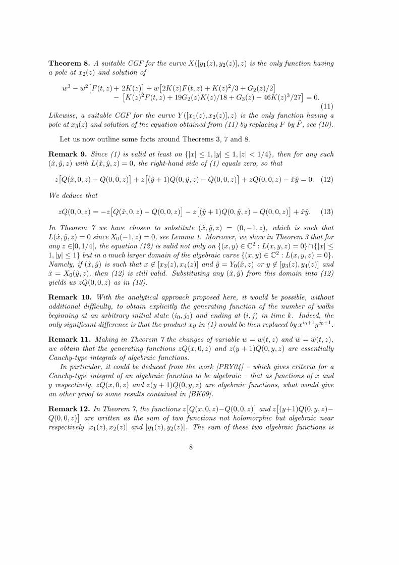
We are now going to transform this integral representation of zQ(x, 0, z). To beginwith, let C(ǫ, z) be any contour such that

(i) C(ǫ, z) is connected and contains ∞,

(ii) C(ǫ, z) ⊂(GX([y1(z), y2(z)], z) ∪X([y1(z), y2(z)], z)

)\ [x1(z), x2(z)],

(iii) limǫ→0C(ǫ, z) = X([y1(z), y2(z)], z) ∪ S(z), where we have denoted by S(z) thesegment [x1(z),X(y2(z), z)] traversed from X(y2(z), z) to x1(z) along the lower edgeof the slit and then back to X(y2(z), z) along the upper edge,

and let GC(ǫ, z) be the connected component of 0 of C \ C(ǫ, z).

9

ε

1 (z) 2x (z)

(z)y1 y2 (z)

3 4x x(z) (z)

],z),X([ C( ,z)

x

Figure 3: The curve X([y1(z), y2(z)], z) and the new contour of integration C(ǫ, z)

Now we apply the residue theorem to the integrand of (14) on the contour C(ǫ, z). Asa function of t, tY0(t, z) is holomorphic GC(ǫ, z), thanks to Lemma 1 and the property (ii)of the contour. Likewise, by using Definition 6 and the property (ii), we get that∂tw(t, z)/(w(t, z) − w(t, x)) is meromorphic on GC(ǫ, z), with a unique pole at t = x.Therefore we have :

1

2πı

∫

C(ǫ,z)tY0(t, z)

∂tw(t, z)

w(t, z) − w(x, z)dt = xY0(x, z). (15)

Then, making ǫ go to 0, using (14), (15) and the property (iii) of the contour, we obtainthat up to an additive function of z,

zQ(x, 0, z) = xY0(x, z) −1

2πı

∫

S(z)tY0(t, z)

∂tw(t, z)

w(t, z) − w(x, z)dt. (16)

Since the integrand in (16) is holomorphic at any point of ]x2(z),X(y2(z), z)[, we have

∫

S(z)tY0(t, z)

∂tw(t, z)

w(t, z) − w(x, z)dt =

∫ x2(z)

x1(z)

[tY +

0 (t, z) − tY −0 (t, z)

] ∂tw(t, z)

w(t, z) − w(x, z)dt,

(17)so that with (3) we immediately obtain the expression of z[Q(x, 0, z) − Q(0, 0, z)] statedin Theorem 7.

Likewise, we could obtain the expression of z[(y + 1)Q(0, y, z) −Q(0, 0, z)] written inTheorem 7. The formula for the Q(0, 0, z) has been already proven in Remark 9.

Acknowledgments. We thank Philippe Bougerol for putting our attention to the recentcombinatorial problems and results. We thank Amaury Lambert for suggesting us to studyMireille Bousquet-Melou papers.

10

1 Study of the conformal gluing function

Notation. For the sake of shortness we will, from now on, drop the dependence of thedifferent quantities w.r.t. z ∈]0, 1/4[.

The main subject of Section 1 is to prove Theorem 8. In other words, we will provethat the CGF proposed in [FIM99] satisfy the conclusions of Theorem 8.

This definition of the CGF given in [FIM99] is recalled here in Subsection 1.2, seeparticularly (24) and (25). It uses some functions defined on a uniformization of thealgebraic curve (x, y) ∈ C

2 : L(x, y, z) = 0, so that we begin Section 1 by studying thisuniformization ; this Subsection 1.1 is also necessary in Section 2, where we will proveTheorem 3.

1.1 Uniformization

We will note L the algebraic curve (x, y) ∈ C2 : L(x, y, z) = 0, L being defined in (1).

Proposition 13. For any z ∈]0, 1/4[, L is a Riemann surface of genus one.

Proof. We have shown in Section 0 that L(x, y, z) = 0 if and only if (b(x)+2a(x)y)2 = d(x).But the Riemann surface of the square root of a polynomial which has four distinct rootsof order one has genus one, see e.g. [JS87], therefore the genus of L is also one.

With Proposition 13 it is immediate that L is isomorphic to some torus ; in otherwords there exists a two-dimensional lattice Ω such that L is isomorphic to C/Ω. Asuitable lattice Ω (in fact the only possible lattice, up to a homothetic transformation) ismade explicit in Parts 3.1 and 3.3 of [FIM99], namely ω1Z + ω2Z, where

ω1 = ı

∫ x2

x1

dx

[−d(x)]1/2, ω2 =

∫ x3

x2

dx

[d(x)]1/2. (18)

We are now going to give a uniformization of the surface L , in other words we willmake explicit two functions x(ω), y(ω) elliptic w.r.t. the lattice Ω such that L =(x(ω), y(ω)), ω ∈ C = ((x(ω), y(ω)), ω ∈ C/Ω). By using the same arguments asin Part 3.3 of [FIM99], we immediately obtain that we can take

x(ω) = x4 +d′(x4)

℘(ω) − d′′(x4)/6, y(ω) =

1

2a(x(ω))

[−b(x(ω)) +

d′(x4)℘′(ω)

2(℘(ω) − d′′(x4)/6)2

],

(19)℘ being the Weierstrass elliptic function with periods ω1, ω2.

By convenience, we will consider from now on that the coordinates of the uniformizationx and y are defined on C/Ω rather than on C.

It is well-known that ℘ is characterized by its invariants g2, g3 through

℘′(ω)2 = 4℘(ω)3 − g2℘(ω) − g3. (20)

11

Lemma 14. The invariants g2, g3 of ℘ are equal to :

g2 = (4/3)(1 − 16z2 + 16z4

), g3 = −(8/27)

(1 − 8z2

)(1 − 16z2 − 8z4

).

Proof. It is well-known that 4℘(ω)3 − g2℘(ω) − g3 = 4(℘(ω) − ℘(ω1/2)

)(℘(ω) − ℘((ω1 +

ω2)/2))(℘(ω) − ℘(ω2/2)

); in particular the invariants can be calculated in terms of the

values of ℘ at the half-periods. But it is proved in Part 3.3 of [FIM99] that settingf(t) = d′(x4)/(t − x4) + d′′(x4)/6 we have ℘(ω1/2) = f(x3), ℘((ω1 + ω2)/2) = f(x2) and℘(ω2/2) = f(x1), so that Lemma 14 follows from a direct calculation.

Now that the uniformization (19) is completely and explicitly defined, it is natural tobe interested in how it transforms the important cycles that are the branch cuts [x1, x2],[x3, x4], [y1, y2] and [y3, y4]. For this we need to define a new period, namely

ω3 =

∫ x1

−∞

dx

[d(x)]1/2. (21)

We will importantly use the fact that ω3 ∈]0, ω2[ – this is proved in Part 3.3 of [FIM99].

Proposition 15. We have x−1([x1, x2]) = [0, ω1[+ω2/2 and x−1([x3, x4]) = [0, ω1[,y−1([y1, y2]) = [0, ω1[+(ω2 + ω3)/2 and y−1([y3, y4]) = [0, ω1[+ω3/2.

Proposition 15 follows from repeating some arguments in Part 5.5 of [FIM99], and isillustrated on Figure 4 below.

Now we define S(x, y) = 1/x + 1/(xy) + x + xy, the generating function of the jumpprobabilities of Gessel’s walk, and we consider the following birational transformations :

Ψ(x, y) =(x, 1/(x2y)

), Φ(x, y) =

(1/(xy), y

). (22)

They are such that S Ψ = S Φ = S. Then, as in [FIM99], we define the groupof the random walk as the group G generated by Ψ and Φ. This is well known, seee.g. [BMM08], that G is of order eight for the process considered here : in other wordsinfn ∈ N : (Φ Ψ)n = id = 4.

If (x, y) ∈ C2 is such that L(x, y, z) = 0 and if θ is any element of G, then

L(θ(x, y), z) = 0. In other words the group G can also be understood as a group ofautomorphisms of the algebraic curve L .

It is also shown in Part 3.1 of [FIM99] that the automorphisms Ψ and Φ defined onL become on C/Ω the automorphisms ψ and φ with the following expressions :

ψ(ω) = −ω, φ(ω) = −ω + ω3. (23)

They are such that ψ2 = φ2 = id, x ψ = x and y φ = y. A crucial fact is the following.

Proposition 16. For all z ∈]0, 1/4[, we have ω3 = 3ω2/4.

12

Proof. Since the group generated by Ψ and Φ is of order eight, so is the group generatedby ψ and φ, in other words infn ∈ N : (φ ψ)n = id = 4. With (23) this immediatelyimplies that 4ω3 is some point of the lattice Ω. But we already know that ω3 ∈]0, ω2[ sothat two possibilities remain : either ω3 = ω2/4 or ω3 = 3ω2/4.

In addition, essentially because the covariance of Gessel’s walk is positive, we canrepeat the same arguments as in Section 4 of [KR09] (see page 14) and in this way weobtain that ω3 is necessary larger than ω2/2, which entails Proposition 16.

1.2 Implicit expression of the CGF

As said in Section 0, the existence of CGF for the curves X([y1, y2]) and Y ([x1, x2]) followsfrom general results on conformal gluing ; actually finding explicit expressions for CGF ismore problematic.

But by using the same arguments as in Part 5.5 of [FIM99], we obtain that the followingfunction is a suitable CGF for X([y1, y2]) :

w(t) = ℘1,3

(x−1(t) − (ω1 + ω2)/2

), (24)

℘1,3 being the Weierstrass elliptic function with periods ω1, ω3 and x−1 the reciprocalfunction of the first coordinate of the uniformization (19) ; the periods ω1, ω2, ω3 aredefined in (18) and (21).

In Section 4 of [KR09], we have studied some properties of the function (24), and wehave shown that since ω3 > ω2/2 (we recall from Proposition 16 that ω3 = 3ω2/4), thefunction (24) is in fact meromorphic on C \ [x3, x4] and has there a unique pole, at x2.

In order to find explicitly a CGF for the curve Y ([x1, x2]), we remark that

w(t) = w(X0(t)) (25)

is suitable – this is a consequence of the facts that w is a CGF for X([y1, y2]) and thatX0 : GY ([x1, x2]) \ [y1, y2] → GX([y1, y2]) \ [x1, x2] is conformal, as stated in Lemma 17.

More globally, w defined by (25) is meromorphic on C\ [y3, y4], and has there a uniquepole, of order two and at Y (x2) = x3 – this is a consequence of some properties of walready mentioned and of the fact that X0(C) ⊂ C \ [x3, x4], see Lemma 17 below.

Lemma 17. X0 : GY ([x1, x2]) \ [y1, y2] → GX([y1, y2]) \ [x1, x2] and Y0 : GX([y1, y2]) \[x1, x2] → GY ([x1, x2]) \ [y1, y2] are conformal and reciprocal the one from the other. Inaddition, X0(C) ⊂ C \ [x3, x4] and Y0(C) ⊂ C \ [y3, y4]

For the proof of Lemma 17, we refer to Part 5.3 of [FIM99].

1.3 Proof of Theorem 8

Proof of Theorem 8. In this proof, we are going here to note ω4 = ω2/4 and ℘1,4 theWeierstrass elliptic function with periods ω1, ω4. Moreover, we recall that ℘ and ℘1,3 arethe Weierstrass elliptic functions with respective periods ω1, ω2 and ω1, ω3 = 3ω2/4.

13

To begin with, let us mention the following fact. Let ℘ be the Weierstrass ellipticfunction with periods noted ω, ω and let n be some positive integer. Then the Weierstrasselliptic function with periods ω, ω/n can be written in terms of ℘ as follows (see e.g.http://functions.wolfram.com/EllipticFunctions/WeierstrassP/16/06/03/) :

℘(ω) +

n−1∑

k=1

[℘(ω + kω/n) − ℘(kω/n)

]. (26)

Then, by using e.g. the addition theorem (27) for the Weierstrass elliptic function ℘ in (26)and next (20), we obtain that the Weierstrass elliptic function with periods ω, ω/n is arational function of the Weierstrass elliptic function with periods ω, ω.

The proof of Theorem 8 will follow from applying this fact twice : (i) first, sinceω4 = ω2/4, we will express ℘1,4 as a rational function of ℘, (ii) then, since ω4 = ω3/3, wewill express ℘1,4 as a rational function of ℘1,3.

Before making explicit the rational transformations that appear in (i) and (ii), weexplain how to conclude the proof of Theorem 8. An immediate consequence of (i)and (ii) is the possibility of writing ℘1,3 as an algebraic function of ℘. In particular,it is immediate from that and from the addition theorem (27) for ℘ that the formulaw(t) = ℘1,3

(℘−1(f(t)) − (ω1 + ω2)/2

), with f(t) = d′(x4)/(t − x4) + d′′(x4)/6 – which is

the CGF under consideration, see (19) and (24) – defines an algebraic function of t.

Explicit expression of the rational function for (i). With (26) we can write

℘1,4(ω) = ℘(ω)+℘(ω+ω2/2)+℘(ω+ω2/4)+℘(ω+3ω2/4)−℘(ω2/2)−℘(ω2/4)−℘(3ω2/4).

Then, by using the addition theorem for ℘, namely the following formula, valid for allω, ω, that can be found e.g. in [Law89],

℘(ω + ω

)= −℘

(ω) − ℘

(ω)

+1

4

[℘′

(ω)− ℘′

(ω)

℘(ω)− ℘

(ω)

]2

, (27)

as well as the equalities ℘(ω2/4) = ℘(3ω2/4), ℘′(ω2/4) = −℘′(3ω2/4) and ℘′(ω2/2) = 0

– obtained from the facts that ℘(ω2/2 + ω) is even and ℘′(ω2/2 + ω) is odd –, we get

℘1,4(ω) = −2℘(ω)+℘′(ω)2 + ℘′(ω2/4)

2

2[℘(ω) − ℘(ω2/4)

]2 +℘′(ω)2

4[℘(ω) − ℘(ω2/2)

]2−℘(ω2/2)−2℘(ω2/4). (28)

We recall from the proof of Lemma 14 that ℘(ω2/2) = f(x1). In other words, for theright-hand side of (28) to be completely explicit, it remains to find the expression ℘(ω2/4)and ℘′(ω2/4) in terms of z. Starting from the known value of ℘(ω2/2), it is easy to

14

obtain the value of ℘(ω2/4), by using e.g. the formula below (a proof of which being givenin [Law89]) :

℘ (ω2/4) = ℘ (ω2/2) +[(℘ (ω2/2) − ℘ (ω1/2)) (℘ (ω2/2) − ℘ ((ω1 + ω2)/2))

]1/2. (29)

Then we use that ℘(ω1/2) = f(x3), ℘((ω1 + ω2)/2) = f(x2), and after simplification weobtain ℘(ω2/4) = (1 + 4z2)/3. As a consequence and with (20) and Lemma 14, we get℘′(ω2/4) = −8z2. In conclusion, the right-hand side of (28) is completely known.

In particular, evaluating (28) at ω = ℘−1(f(t)) − (ω1 + ω2)/2 and using again theaddition formula (27) for ℘, we obtain that the right-hand side of (28) is a rational functionof t that can be explicitly obtained in terms of t and z ; after a substantial but elementarycalculation we get ℘1,4

(℘−1(f(t)) − (ω1 + ω2)/2

)= F (t), F being defined in (10).

Explicit expression of the rational function for (ii). Using the same arguments that haveallowed us to obtain (28) from (26), we obtain that ℘1,4 is the following rational functionof ℘1,3 :

℘1,4(ω) = −℘1,3(ω) +℘′

1,3(ω)2 + ℘′1,3(ω3/3)

2

2[℘1,3(ω) − ℘1,3(ω3/3)

]2 − 4℘1,3(ω3/3). (30)

By using (30) and the equality ℘′1,3(ω)2 = 4℘1,3(ω)3−g2,1,3℘1,3(ω)−g3,1,3, where g2,1,3, g3,1,3

are the invariants associated with ℘1,3, we get that ℘1,4 is a rational function of ℘1,3 ;moreover, with Lemma 18, the equality ℘′

1,3(ω3/3)2 = 4℘1,3(ω3/3)

3−g2,1,3℘1,3(ω3/3)−g3,1,3

and Lemma 19, the coefficients of this rational function in terms of z are explicitly known.

Proof of (11). Now we remark that with Lemmas 18 and 19, (30) can be written as

℘1,3(ω)3 − ℘1,3(ω)2[℘1,4(ω) + 2K

]+ ℘1,3(ω)

[2K℘1,4(ω) +K2/3 +G2/2

]

−[K2℘1,4(ω) + 19G2K/18 +G3 − 46K3/27

]= 0.

In particular, evaluating this equality at ω = ℘−1(f(t)) − (ω1 + ω2)/2, using the factalready proved that ℘1,4

(℘−1(f(t))− (ω1 + ω2)/2

)= F (t) as well as the definition (24) of

w, we obtain (11).

End of the proof of Theorem 11. If F is infinite at some point, then the equality (11)becomes (w−K)2 = 0. In particular, at a such point at least two roots of (11) take finitevalues. In addition, by using the root-coefficient relationships, it is clear that at a pointwhere F is infinite, at least one root of (11) is infinite. This proves that at any pointwhere F is infinite, there is one and only one root of (11) which is infinite.

In particular, since F is infinite at x2, see (10), and since w has a pole at x2, seeSubsection 1.2, w can be characterized as the only solution of (11) with a pole at x2.

Likewise, we could prove the corresponding fact for w. Theorem 11 is proved.

Let G2, G3,K be the quantities defined in Section 0, above Theorem 8.

Lemma 18. ℘1,3(ω3/3) = K.

15

Lemma 19. g2,1,3, g3,1,3, the invariants of ℘1,3, have the following explicit expressions :

g2,1,3 = 40K2/3 −G2, g3,1,3 = −280K3/27 + 14KG2/9 +G3.

Proof of Lemmas 18 and 19. Start by expanding ℘1,4 at 0 in two different ways. Firstly,by using (28) and by simplifying, we obtain :

℘1,4(ω) = ω−2 +[9G2/20

]ω2 −

[27G3/28

]ω4 +O(ω6). (31)

Secondly, we can also use (30) and after some calculation we get :

℘1,4(ω) = ω−2+[6K2−9g2,1,3/20

]ω2+

[10K3−3Kg2,1,3/2−27g3,1,3/28

]ω4+O(ω6). (32)

Lemma 19 follows immediately, by identifying the expansions (31) and (32).As for Lemma 18, it will be a consequence of Lemma 19 and of the following result,

proved e.g. in [Law89] : the quantity K = ℘1,3(ω3/3) is the only positive solution of thefollowing equation : K4 − g2,1,3K

2/2 − g3,1,3K − g22,1,3/48 = 0. But thanks to Lemma 19,

we can replace g2,1,3 and g3,1,3 by their expression in terms of K ; in this way we obtainthat K verifies the equation K4 −G2K

2/2 −G3K −G22/48 = 0.

2 Holomorphic continuation of zQ(x, 0, z) and z(y+1)Q(0, y, z)

In this part we are going to prove Theorem 3, in other words we are going to show thatzQ(x, 0, z) and z(y + 1)Q(0, y, z) can be holomorphically continued up to C \ [x3, x4] andC \ [y3, y4] respectively.

In fact, we are going to show that Q(x, 0, z) and Q(0, y, z) can be holomorphicallycontinued up to C \ [x3, x4] and C \ [y3, y4] respectively, which is an equivalent assertion,since as said in Section 0, Q(0, y, z) is bounded at −1.

For this we will use the following procedure :

(i) First, we will lift the functions Q(x, 0, z) and Q(0, y, z) up to C/Ω by settingqx(ω) = Q(x(ω), 0, z) and qy(ω) = Q(0, y(ω), z). The functions qx and qy are apriori well defined on x−1(|x| ≤ 1) and y−1(|y| ≤ 1) respectively.

(ii) Then, we will prove the following.

Theorem 20. qx and qy, initially well defined on x−1(|x| ≤ 1) and y−1(|y| ≤ 1)respectively, can be holomorphically continued up to the whole parallelogram C/Ω cut alongrespectively [0, ω1[ and [0, ω1[+ω3/2. Moreover, these continuations verify

∀ω ∈ C/Ω \ [0, ω1[ : qx(ω) = qx(ψ(ω)), ∀ω ∈ C/Ω \([0, ω1[+ω3/2

): qy(ω) = qy(φ(ω)),

(33)and

∀ω ∈]3ω2/8, ω2[×[0, ω1/ı[ : zqx(ω) + z(y(ω) + 1)qy(ω)− zQ(0, 0, z)−x(ω)y(ω) = 0. (34)

16

(iii) Finally, we will set Q(x, 0, z) = qx(ω) if x(ω) = x and Q(0, y, z) = qy(ω) if y(ω) = y.Thanks to (33) and Proposition 15, these relations define Q(x, 0, z) and Q(0, y, z) onrespectively C \ [x3, x4] and C \ [y3, y4] not ambiguously, as holomorphic functions.

Moreover, both (4) and (5) are immediate consequences of (34).

Items (i) and (iii) are straightforward. For the proof of (ii), it will be useful first to findthe location of the cycles x−1(|x| = 1) and y−1(|y| = 1) on C/Ω, this is the subjectof the following result, illustrated on Figure 4 below.

2

|x|<1 _

|y|<1_

4

3 2x

x1x

x y

y

y

y4

3

1

Figure 4: Location of the important cycles on the surface [0, ω2[×[0, ω1/ı[

Proposition 21. We have x−1(|x| = 1) =([0, ω1[+ω2/4

)∪

([0, ω1[+3ω2/4

)and

y−1(|y| = 1) =([0, ω1[+ω2/8

)∪

([0, ω1[+5ω2/8

).

Proof. The details are of course essentially the same for x and y, so that we are going toprove only the assertion concerning x. We are going to show it with three steps.

But first of all we note that because of the equality x ψ = x, it is sufficient to provethat x−1(|x| = 1) ∩

([0, ω2/2] × [0, ω1/ı[

)= [0, ω1[+ω2/4 – the advantage of this being

that ℘, and therefore also x, are one-to-one in [0, ω2/2] × [0, ω1/ı[.Firstly, we prove that x(ω2/4 + ω1/2) = 1. For this we recall from the proof of

Theorem 11 that ℘(ω2/4) = (1 + 4z2)/3. Then with the addition theorem (27) weimmediately obtain the explicit value of ℘(ω2/4 + ω1/2), since the ones of ℘(ω2/4),℘′(ω2/4) = −8z2 and ℘(ω1/2) = f(x3) are known. Finally, after a simple calculationand by using (19), we get x(ω2/4 + ω1/2) = 1.

Secondly, we show that x−1(|x| = 1)∩([0, ω2/2]× [0, ω1/ı[

)⊂ [0, ω1[+ω2/4. For this

let θ ∈ [0, 2π[. With (19) we have x(ω) = exp(ıθ) if and only if ℘(ω) = f(exp(ıθ)). Sinceω ∈ [0, ω2/2] × [0, ω1/ı[, we can use the explicit expression of the reciprocal function of ℘and with the first step we obtain :

ω = ω2/4+ω1/2+

∫ f(exp(ıθ))

f(1)

dt

[4t3 − g2t− g3]1/2= ω2/4+ω1/2+

1

2

∫ 1

exp(ıθ)

dx

[d(x)]1/2, (35)

17

d being the polynomial defined in Section 0. Note that the second equality above is gotwith the same calculations as in Part 3.3 of [FIM99].

Now we remark that d(x) = x4d(1/x). In particular, the change of variable x 7→ 1/x inthe integral

∫ 1exp(ıθ) dx/[d(x)]1/2 yields

∫ 1exp(ıθ) dx/[d(x)]1/2 = −

∫ 1exp(−ıθ) dx/[d(x)]1/2. As

a consequence, this integral belongs to ıR.In conclusion, with (35) we have actually shown that x−1(|x| = 1) ∩

([0, ω2/2] ×

[0, ω1/ı[)⊂ [0, ω1[+ω2/4.

Thirdly, we prove that the inclusion above has to be an equality. Indeed, if it wasnot the case the curve x−1(|x| = 1) ∩

([0, ω2/2] × [0, ω1/ı[

)would be curve not closed,

which is a manifest contradiction with the fact that its image through the function x,meromorphic and one-to-one in [0, ω2/2] × [0, ω1/ı[, namely the unit circle, is a closedcurve.

Proof of Theorem 20. The proof is composed of four steps. We will first, in three items,define the continuations of qx and qy on the whole parallelogram C/Ω appropriately cut.In conclusion we will verify that the functions so constructed actually verify the factsclaimed in the statement of Theorem 20.

• We define qx(ω) on x−1(|x| ≤ 1) by Q(x(ω), 0, z) and qy(ω) on y−1(|y| ≤ 1)by Q(0, y(ω), z). Note that as a consequence of Proposition 21 we have x−1(|x| ≤1) = [ω2/4, 3ω2/4] × [0, ω1/ı[ and y−1(|y| ≤ 1) = [5ω2/8, 9ω2/8] × [0, ω1/ı[.

• Motivated by (1), on [3ω2/4, ω2[×[0, ω1/ı[⊂ y−1(|y| ≤ 1) we set qx(ω) = −(y(ω) +1)qy(ω) +Q(0, 0, z) + x(ω)y(ω)/z and on ]3ω2/8, 5ω2/8] × [0, ω1/ı[⊂ x−1(|x| ≤ 1)we set (y(ω) + 1)qy(ω) = −qx(ω) +Q(0, 0, z) + x(ω)y(ω)/z.

• On ]0, ω2/4] × [0, ω1/ı[ we define qx(ω) by qx(φ(ω)) – note that with (23) we haveφ(]0, ω2/4] × [0, ω1/ı[) = [3ω2/4, ω2[×[0, ω1/ı[ – and on [ω2/8, 3ω2/8[×[0, ω1/ı[ wedefine qy(ω) by qy(ψ(ω)) – by using (23) we have ψ([ω2/8, 3ω2/8[×[0, ω1/ı[) =]3ω2/8, 5ω2/8] × [0, ω1/ı[.

The functions qx and qy are now well defined on the whole parallelogram C/Ω cutalong [0, ω1[ and [0, ω1[+ω3/2 respectively.

Note that the definition given in the first item is quite natural. The one stated in thesecond item is also natural since on x−1(|x| ≤ 1) ∩ y−1(|y| ≤ 1) = [5ω2/8, 3ω2/4] ×[0, ω1/ı[, the equality zqx(ω)+z(y(ω)+1)qy(ω)−zQ(0, 0, z)−x(ω)y(ω) = 0 holds, see (1).The definition set in the third item is to ensure that (33) is valid.

Note also that (34) is immediately true, by construction of the continuations.We are now going to verify (33) for qx. Since x ψ = x, (33) is obviously verified

on [ω2/4, 3ω2/4] × [0, ω1/ı[= ψ([ω2/4, 3ω2/4] × [0, ω1/ı[). Moreover, with the third item,(33) is verified for qx on ]0, ω2/4] × [0, ω1/ı[, and since ψ2 = id, (33) is also true for qx on[3ω2/4, ω2[×[0, ω1/ı[, and finally on the whole C/Ω \ [0, ω1[.

Likewise, we verify easily that (33) is valid for qy on C/Ω \([0, ω1[+3ω2/8

).

18

It remains to prove that the continuations of qx and qy are holomorphic on C/Ω cutalong [0, ω1[ and [0, ω1[+3ω2/8 respectively.

We show first that they are meromorphic on their respective cut parallelogram. Forqx the following cycles are a priori problematic : [0, ω1[, [0, ω1[+ω2/4 and [0, ω1[+3ω2/4.

In an open neighborhood of [0, ω1[+3ω2/4, we have qx(ω) = −(y(ω) + 1)qy(ω) +Q(0, 0, z) + x(ω)y(ω)/z, so that qx is in fact meromorphic in the neighborhood of thecycle [0, ω1[+3ω2/4. Since (33) holds, qx is also meromorphic near [0, ω1[+ω2/4 =ψ([0, ω1[+3ω2/4), so that only [0, ω1[ remains a priori a singular cycle.

Similarly, we could show that qy is meromorphic on C/Ω \([0, ω1[+3ω2/8

).

Let us now prove that these continuations are actually holomorphic on their respectivecut parallelogram.

qx is obviously holomorphic on ]ω2/4, 3ω2/4]×[0, ω1/ı[, since it is there defined throughits power series.

On ]5ω2/8, ω2[×[0, ω1/ı[, we have qx(ω) = −(y(ω) + 1)qy(ω) +Q(0, 0, z) + x(ω)y(ω)/z,and all terms of the right-hand side of this equality are holomorphic on this domain – at7ω2/8, x has a pole of order one and y has a zero of order two so that the product xy isholomorphic near 7ω2/8 (this is a consequence of Lemma 1 that the only poles of x are atω2/8, 7ω2/8, its only zeros are at 3ω2/8, 5ω2/8 and that the only pole of y (of order two)is at 3ω2/8 and its only zero (of order two) is at 7ω2/8).

On ]0, 3ω2/8[×[0, ω1/ı[, we have qx = qx ψ, so that qx is holomorphic on this domainsince it is on ψ(]0, 3ω2/8[×[0, ω1/ı[) =]5ω2/8, ω2[×[0, ω1/ı[.

Likewise, we could show that (y + 1)qy is holomorphic on C/Ω \([0, ω1[+ω3/2

). This

implies that qy is holomorphic on the same set except at the points where y+1 = 0. Thereare two possibilities in order to show that qy is also holomorphic at these points, namelyω2/8 and 5ω2/8.

First, we can use the fact that the generating function Q(0, y, z) is bounded at −1, seeSection 0, so that qy(ω) = Q(0, y(ω), z), being meromorphic and bounded near ω2/8 and5ω2/8, is actually holomorphic at these points.

We can also remark that with (34), (y(5ω2/8) + 1)qy(5ω2/8) = 0, since x(5ω2/8) = 0.Moreover, since φ(5ω2/8) = ω2/8, (y(ω2/8)+1)qy(ω2/8) = 0. In other words, at ω = ω2/8and ω = 5ω2/8, both holomorphic functions (y + 1)qy and (y + 1) have a zero of orderexactly one, it follows immedietaly that qy is holomorphic at ω.

19

References

[Ayy09] Arvind Ayyer. Towards a human proof of Gessel’s conjecture. J. Integer Seq., 12(4):Article09.4.2, 15, 2009.

[BK09] Alin Bostan and Manuel Kauers. The complete generating function for gessel walks is algebraic.Preprint available at http://arxiv.org/abs/0909.1965, pages 1–14, 2009.

[BMM08] Mireille Bousquet-Melou and Marni Mishna. Walks with small steps in the quarter plane.Preprint available at http://arxiv.org/abs/0810.4387, pages 1–34, 2008.

[FIM99] Guy Fayolle, Roudolf Iasnogorodski, and Vadim Malyshev. Random walks in the quarter-plane,volume 40 of Applications of Mathematics (New York). Springer-Verlag, Berlin, 1999. Algebraicmethods, boundary value problems and applications.

[Ges86] Ira M. Gessel. A probabilistic method for lattice path enumeration. J. Statist. Plann. Inference,14(1):49–58, 1986.

[JS87] Gareth A. Jones and David Singerman. Complex functions. Cambridge University Press,Cambridge, 1987. An algebraic and geometric viewpoint.

[KKZ09] Manuel Kauers, Christoph Koutschan, and Doron Zeilberger. Proof of ira gessel’s lattice pathconjecture. Proceedings of the National Academy of Sciences, 106(28):11502–11505, 2009.

[KR09] Irina Kurkova and Kilian Raschel. Random walks in (Z+)2 with non-zero drift absorbed atthe axes. Preprint available at http://arxiv.org/abs/0903.5486, pages 1–29. To appear inBulletin de la Societe Mathematiques de France in 2010, 2009.

[Law89] Derek F. Lawden. Elliptic functions and applications, volume 80 of Applied MathematicalSciences. Springer-Verlag, New York, 1989.

[Lit00] Georgii S. Litvinchuk. Solvability theory of boundary value problems and singular integralequations with shift, volume 523 of Mathematics and its Applications. Kluwer AcademicPublishers, Dordrecht, 2000.

[Pin09] Sun Ping. A probabilistic approach to enumeration of gessel walks. Preprint available athttp://arxiv.org/abs/0903.0277, pages 1–14, 2009.

[PRY04] F. Pakovich, N. Roytvarf, and Y. Yomdin. Cauchy-type integrals of algebraic functions. IsraelJ. Math., 144:221–291, 2004.

[PW08] Marko Petkovsek and Herbert Wilf. On a conjecture of ira gessel. Preprint available athttp://arxiv.org/abs/0807.3202, pages 1–11, 2008.

20