WP/04/140

Explaining Efficiency Differences Among Large German and Austrian Banks

David Hauner

© 2004 International Monetary Fund WP/04/140

IMF Working Paper

African Department

Explaining Efficiency Differences Among Large German and Austrian Banks

Prepared by David Hauner1

Authorized for distribution by Francesco Caramazza

August 2004

Abstract

This Working Paper should not be reported as representing the views of the IMF. The views expressed in this Working Paper are those of the author(s) and do not necessarily represent those of the IMF or IMF policy. Working Papers describe research in progress by the author(s) and are published to elicit comments and to further debate.

Cost-efficiency, scale efficiency, and productivity change are estimated by data envelopmentanalysis; and cost-efficiency is regressed on explanatory variables. No evidence is found for average productivity responding to deregulation over the period studied. State-owned banks are found to be more cost-efficient (likely owing to cheaper funds) and cooperative banks to be about as cost-efficient as private banks. Increasing economies of scale but decreasing economies of scope provide rationale for M&As among banks with similar product portfolios. Interbank and capital market funding is found to be more cost-efficient than deposits when the cost of retail networks is controlled for. JEL Classification Numbers: G21, G34 Keywords: Banks, efficiency, Germany, Austria, data envelopment analysis Author’s E-Mail Address: dhauner@imf.org

1 The author thanks Georg Winckler and Jörg Finsinger at the University of Vienna; Harald Stieber at the Organization for Economic Cooperation and Development (OECD); Edward Vytlacil at Stanford University; Laurent P. Bouscharain, Allan David Brunner, Francesco Caramazza, Jorg Decressin, and Thomas Walter at the IMF; Gertrude Tumpel-Gugerell at the European Central Bank; and Josef Christl and Peter Zöllner at the Austrian National Bank. Of course, the author is responsible for any remaining errors.

- 2 -

Contents Page

I. Introduction ............................................................................................................................3

II. Overview of Selected Prior Studies ......................................................................................4

III. Methodology........................................................................................................................5

IV. Model and Data..................................................................................................................12

V. Data Envelopment Analysis (DEA) Results .......................................................................13

VI. Explaining Differences in Cost-Efficiency........................................................................16

VII. Conclusions ......................................................................................................................20

References................................................................................................................................21 Tables 1. Input and Output Quantities and Input Prices—Descriptive Statistics................................13 2. Cost-Efficiency: Summary of DEA Results ........................................................................14 3. Cost-Efficiency (Mean): Decomposition into Technical and Allocative Efficiency ..........14 4. Cost-Efficiency (1995–99 Mean) by Size and Market ........................................................15 5. Scale Efficiency: Summary of DEA Results .......................................................................15 6. Scale Efficiency (Pooled 1995–99 Mean), by Size and Market ..........................................15 7. Productivity Change 1995–99: Summary of Malmquist Decomposition............................16 8. Net Productivity Change 1995–99 (Geometric Means)—Malmquist Decomposition by

Market and Size ...............................................................................................................16 9. Explanatory Variables: Definitions and Descriptive Statistics............................................17 10. Regression Results—Factors Explaining Differences in Cost-Efficiency.........................18 Figures 1. Technical Efficiency and Scale Efficiency ........................................................................6 2. Technical Efficiency and Allocative Efficiency ................................................................7

- 3 -

I. INTRODUCTION

This study examines the sources of efficiency2 differences among large3 German and Austrian commercial banks. First, measures of their cost-efficiency, scale efficiency, and productivity change are estimated by data envelopment analysis (DEA). Cost-efficiency averages 63 percent, and scale efficiency averages 96 percent. There is no evidence for average productivity responding to deregulation over the period studied. Second, cost-efficiency is regressed on a number of variables, yielding three major results: State-owned banks are found to be more cost-efficient (likely owing to access to cheaper funds thanks to state guarantees) and cooperative banks to be about as cost-efficient as private banks. The finding of increasing economies of scale but decreasing economies of scope provides rationale for mergers and acquisitions among banks with similar product portfolios. Interbank and capital market funding is found to be more cost-efficient than deposits when the cost of retail networks is controlled for. Very few studies (e.g., Berger and Mester, 1997a) and, to the author’s knowledge, none for German and Austrian banks have examined the sources of efficiency differences. And of those that did, only a handful have gone beyond simple comparisons of average efficiency scores by various subsamples (e.g., according to size or ownership). Such simple comparisons are prone to a potentially serious omitted-variable bias, a shortcoming avoided by the econometric analysis undertaken here. Policy-wise, this paper is motivated by the ongoing dramatic structural changes in the European banking sectors. The European Union (EU) single market for financial services and the common currency have removed the last major obstacles to cross-border competition in financial services. In addition, financial innovation and increased competition from non-EU banks and nonbank financial institutions is putting EU banks under pressure to improve their efficiency. In addition to that, German and Austrian banks are faced with important structural changes in their home markets. Most prominently, in Germany, state guarantees (for the commercial bank activities) of Sparkassen (savings banks) and their larger clearing institutions, the Landesbanken, will expire in July 2005. And the creation of the legal framework to “reduce barriers to consolidation, within or across pillars [private, public, and cooperative banks] and thereby facilitate market-oriented restructuring,” as called for (not only) in IMF (2003) is likely to result in yet another consolidation wave in a market that is still widely considered

2 Efficiency is used here as a relative concept, i.e., the distance of a bank from a frontier formed by best performers (see Section III).

3 “Large” relative to the average German and Austrian bank. This paper is limited to large banks because frontier analysis rests on the assumption that the sample banks are indeed comparable in their business model. Therefore, a larger span between the largest and the smallest banks in the sample introduces more bias in the estimation. The potential bias introduced by pooling banks from different countries is arguably minimal here because the Austrian and German banking systems are extremely similar in their structure, and the Austrian banking sector is to a high degree owned by German institutions.

- 4 -

overbanked and populated by many institutions that are arguably not primarily profit maximizing.4 In what follows, Section II reviews prior studies. Section III presents the methodology; Section IV discusses model and data; Section V presents the DEA results; and Section VI the regression analysis of cost-efficiency. Section VII concludes.

II. OVERVIEW OF SELECTED PRIOR STUDIES

Research on bank productivity ballooned in the 1990s, triggered not least by the deregulation of the US banking industry in the 1980s. In their review, Berger and Humphrey (1997) count 130 studies on the efficiency of financial institutions in 21 countries; 116 of them were published in the years 1992 to 1997. The median of efficiency estimates for the U.S. banking system amounts to around 80 percent. While cost inefficiency therefore seems to be substantial, scale inefficiency in U.S. banking has frequently been found to be negligible. In their review, Berger, Hunter, and Timme (1993) put the typical estimate at around 5 percent. Some papers on the U.S. banking system examine policy issues similar to this study. Berger and Humphrey (1991) find that, despite heavy deregulation activity during the period examined, productivity did not improve substantially. Alam (2001) finds that deregulation takes several years to translate into productivity improvements. Fixler and Zieschang (1993) find that—even though acquiring banks do not improve their individual efficiency—acquisitions improve systemwide efficiency because the acquiring banks are on average more efficient than the acquired banks. Peristiani (1996) finds that the average acquiring bank experiences a small but significant efficiency loss in the first two to four years after the acquisition. Berger and Hannan (1998) find support for Hicks’s “quiet life hypothesis,” which predicts a negative relation between market concentration (as a proxy for competition) and efficiency. Studies of European banking sectors, like those of the American, generally find that cost inefficiency by far outweighs scale inefficiency. However, estimates of average cost-efficiency varies considerably across countries. To cite a few examples, Sheldon (1994), Favero and Papi (1995), Grifell-Tatjé and Lovell (1997), Resti (1997), and Maudos and Pastor (2003) study the efficiency of the Swiss, Italian, Spanish, Italian, and Spanish banking systems, respectively. Various studies comparing the German and Austrian banking systems to others find efficiency in those two markets in the order of 75 to 90 percent.5 Allen and Rai (1996)

4 Small savings banks and cooperative banks in aggregate have an overwhelming market share, with the remaining share accounted for by the third “pillar” of private sector banks. Assets of the average German bank were only 67 percent of the average French bank’s and 56 percent of the average Spanish bank’s in 2001. After-tax profit was on average 0.2 percent of total assets in Germany, but 0.7 percent in France, 0.9 percent in Spain, and 1.0 percent in Italy, according to Brunner and others (2003). See their paper for a detailed discussion of the German banking system.

- 5 -

examine the German and Austrian banking systems within a panel of banks in 24 countries over the years 1988 to 1992 and find that efficiency averaged around 88 (89) percent for the German (Austrian) banks included in the sample. In a 10-country study, Pastor, Pérez, and Quesada (1997) put average efficiency for 22 (45) German (Austrian) banks at around 80 (50) in 1992. Vennet (2002) finds efficiency in the range of 68 to 82 percent, depending on the model and subsample he uses. Pastor (2002) finds average efficiency of 42 percent for the German banks in a study of several European markets with a model that includes credit risk and environmental variables. Studies focusing exclusively on various samples of German banks find average cost-efficiency in the order of 80 percent.3 Altunbas, Evans, and Molyneux (1997) find for 196 large and medium-sized banks an average cost-efficiency of around 75 percent. Lang and Welzel (1996) put average cost-efficiency for Bavarian cooperative banks at around 80 percent. Altunbas, Evans, and Molyneux (2001) find average cost-efficiency for the banking sector in the range of 81 to 87 percent, depending on the estimation technique. Brunner and others (2003) find that German banks are not significantly less cost-efficient than those in other European markets, but are still less profitable due to weaker revenue.

III. METHODOLOGY

The theoretical foundations of this study were laid by Debreu (1951), Koopmans (1951), and Farrell (1957), and were extended, in particular, by Färe, Grosskopf and Lovell (1985 and 1994). To the latter, the reader is referred to for a more extensive treatment of the concepts underlying this study, which can only be sketched briefly here. As defined for the purposes of this study, cost-efficiency is composed of technical efficiency, scale efficiency and allocative efficiency. Technical efficiency measures the ability of a bank to produce a given set of outputs with minimal inputs, independently of input prices and under the assumption of variable returns to scale. Scale efficiency measures whether a bank produces at an optimal size of scale. Allocative efficiency measures the ability of a bank to choose optimal input proportions at given input prices.6

5 In the paragraph on prior studies of exclusively German banks, care is taken to distinguish cost efficiency and technical efficiency. The rest of Section II omits this distinction for the sake of easier presentation. The resulting imprecision is dwarfed by the biases arising from the use of different estimation techniques and models that limit the comparability of results.

6 Empirical applications necessarily nearly always refer to relative, absolute (extended Pareto-Koopmans) efficiency. When outputs are held fixed and inputs are to be minimized, relative efficiency is attained by a production unit if and only if according to the available evidence none of the inputs can be reduced without increasing at least another input.

- 6 -

Figure 1. Technical Efficiency and Scale Efficiency

An example in Figure 1 illustrates technical efficiency and scale efficiency. Say, one input x is used to produce one output y. CRS is the production possibilities frontier at constant returns to scale, VRS is the production possibilities frontier at variable returns to scale, and NIRS is the production possibilities frontier at non-increasing returns to scale. Therefore, in the example shown in Figure 1 technical efficiency under constant returns to scale is

TCRS = CA

AC

PxxP λλ

=)( , ( 1 )

technical efficiency under variable returns to scale is

TVRS = VA

AV

PxxP λλ

=)( , ( 2 )

and scale efficiency is

S = )()(

AV

AV

xPxP

λλ , ( 3 )

whereλ are the distances shown in Figure 1.

VRS

P

0

CRSNIRS

y

x

λVxA xAλCxA

VRS

P

0

CRSNIRS

y

x

λVxA xAλCxA

- 7 -

As

(()()(

V

CA

AV

A

AC

xPxP

PxxP

PxxP

λλλλ

⋅=

( 4 )

holds, it follows that

S T T VRSCRS ⋅= . ( 5 )

Returns to scale are increasing if it holds that

CRSVRSNIRSVRS TT T T ≠∧= , ( 6 )

and, in turn, returns to scale are decreasing if it holds that

CRSVRSNIRSVRS TTTT ≠∧≠ . ( 7 )

Figure 2. Technical Efficiency and Allocative Efficiency

x1 L(y)

xAxE

x2

λxA

0

x1 L(y)

xAxE

x2

λxA

0

- 8 -

An example in Figure 2 illustrates the concepts of technical efficiency (at constant returns to scale) and allocative efficiency. The cost-minimizing input vector xE is situated at the tangential point of the isoquant L(y) that permits the production of output y and the slope of the input price ratio. Given an input price vector w, efficient total costs are c(y,w) = wTxE. For input vector xA, cost-efficiency therefore is

AT

ET

ET xwxw

xwwyc C ==

),( , ( 8 )

technical efficiency is

λλ== AT

AT

xwxwT )( , ( 9 )

and allocative efficiency is

)( AT

ET

xwxw

TCA

λ== , ( 10 )

where λ is a scalar. To calculate the various efficiency scores, an empirical frontier (equivalent to the isoquant of an unknown fully technically efficient bank) is estimated. A bank is technically efficient if it lies on the frontier. Otherwise, an efficient projection point on the frontier is calculated as a linear combination of the efficient production sets of benchmark banks with output quantities of similar size as the ones of the inefficient bank.

To establish the frontiers, we use the linear programming-based DEA approach, as it is more adept than parametric approaches at describing frontiers as opposed to central tendencies.7 Instead of trying to fit a regression plane through the center of the data, DEA constructs a piecewise linear surface that connect the set of the best-practice producers, yielding a convex production possibilities set. Under cost minimization (in contrast to output maximization), the best-practice producers are those for which there is no linear combination of producers that use as little or less of each cost component, given output quantities.8

7 The most common parametric approaches are the stochastic frontier approach (SFA), the thick frontier approach (TFA), and the distribution-free approach (DFA). The main trade-off between parametric and non-parametric approaches concerns their assumptions on random errors and the functional form of the cost frontier. While DEA fails to distinguish between inefficiency and random errors, it does presume a particular functional form of the frontier. Parametric approaches, in turn, distinguish between random errors and inefficiency, but do so along the lines of somewhat arbitrary assumptions about their respective distributions, and, in addition, impose a particular functional form, which, if misspecified, risks overstating inefficiency. In practice, bank efficiency studies use nonparametric and parametric methods similarly frequently (Berger and Humphrey, 1997).

8 For further details on DEA and the Malmquist index, the reader is referred to Seiford and Thrall (1990), and Berg, Forsund, and Jansen (1992), respectively. The DEAP software used here is described in Coelli (1996).

- 9 -

The computation of the various efficiency scores can be briefly sketched as follows: First, technical efficiency under constant returns to scale is calculated. Given an input matrix N and an output matrix M, the feasible input sets under the assumption of a constant returns technology to scale are

},,,:{)( MJ yxNMyxyL ++ ℜ∈ℜ∈≤≤= φφφ , ( 11 )

whereφ is a scaling vector for the production plans. Let ),( jj yx be the production plan of the jth producer and take 1=iφ if i = j and 0=iφ otherwise, ensuring that )( jj yLx ∈ . The Shephard (1970) distance function of jx from the efficient frontier,

,min )}L(y{λλ:λ),x(yD jjjji ∈= ( 12 )

measures the (radial9) technical efficiency of the production plan (y,x) under the assumption of a constant returns to scale technology and can be calculated for production plan (yj,xj) of production unit j as the solution to the linear programming problem

Jj

Nnxx

Mmyyts

j

jnj

jnj

jjmjjm

,...,1,0

,...,1,

,...,1,..

min,

=≥

=≤

=≤

∑

∑

φ

λφ

φ

λφλ

( 13 )

Second, in order to separate input waste from wrong size of scale, technical efficiency under variable returns to scale is calculated, for which (11) and (13) are amended by adding the restriction 1=∑

jjφ on the scaling vector.

9 A “radial” reduction cuts all inputs by the highest proportion λ possible for all of them at given output levels. After radial reduction, there could be remaining ‘slack’ in some inputs (Farrell efficiency is necessary but not sufficient for Pareto-efficiency.). Here, this problem is circumvented by amending the linear program so that it meets Koopman-efficiency, which also fulfils the Pareto criterion. See Lovell (1993) for a more extensive treatment, and Coelli (1996) on how the software used here solves the problem.

- 10 -

The production technology (11) becomes

M

jjj

J yyxNMyxyL ++ ℜ∈=ℜ∈≤≤= ∑ },1,,,:{)( φφφφ , ( 14 )

the distance function (12) becomes

)},(:min{),( jjjji yLxxyT ∈= λλ ( 15 )

and finally the linear programming problem (13) becomes

.1

,...,1,0

,...,1,

,...,1,..

min

∑

∑

∑

=

=≥

=≤

=≤

jj

j

jnj

jnj

jjmjjm

Jj

Nnxx

Mmyyts

φ

φ

λφ

φ

λλφ

( 16 )

The values of the results of (13) and (15), respectively, are bounded between zero and unity, with a value of unity indicating that jx belongs to the efficient subset of (11) and (14), respectively. Third, scale efficiency is obtained residually from the ratio

),(),(

),( jji

jjijj

i xyTxyD

xyS = . ( 17 )

To determine whether a producer is located in a region of increasing or decreasing returns to scale, based on the logic of (6) and (7), technical efficiency under non-increasing returns to scale is calculated by imposing 1≤∑

jjφ instead of 1=∑

jjφ on the scaling vector.

Fourth, to calculate cost-efficiency, suppose that, in addition to the assumption made for (8), input prices Np +ℜ∈ are given. Thus, (12) becomes

,,...,1)},(:{min),(,

JjyLxxppyP jj

z

jj =∈=φ

( 18 )

and (13) becomes

.,...,1,0

,...,1,

,...,1,..

min,

Jj

Nnxx

Mmyyts

xp

j

jnj

jnj

jjmjjm

njnjx

=≥

=≤

=≤

Σ

∑

∑

φ

λφ

φφ

( 19 )

- 11 -

Assuming that jp and jx are known, and 0>jj xp , the cost-efficiency measure is

.,...,1,),(),,( JjxppuPxpyC jj

jjjjj

i == ( 20 )

Fifth, the measure for allocative efficiency is obtained residually from the ratio

),(

),,(),,( jj

i

jjjijjj

i xyTxpyC

xpyA = . ( 21 )

To sum up, cost-efficiency attains a value of less than unity if and only if at least one of its three components attains a value of less than unity, due to a wrong input mix given input prices [ ),,( jjj

i xpyA ], an inefficient size of scale [ ),( jji xyS ], or technical inefficiency

)],([ jji xyT . Cost-efficiency is decomposed into

),(),(),,(),( jji

jji

jjji

jji xyTxySxpyAxyC ⋅⋅= . ( 22 )

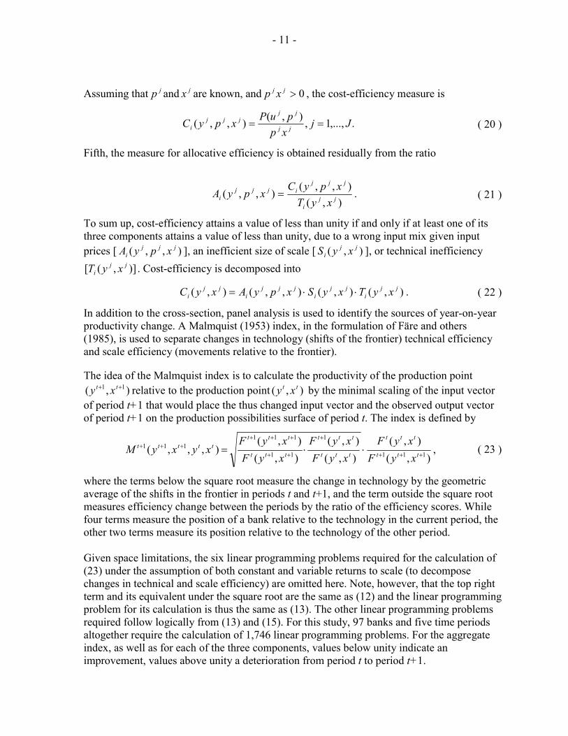
In addition to the cross-section, panel analysis is used to identify the sources of year-on-year productivity change. A Malmquist (1953) index, in the formulation of Färe and others (1985), is used to separate changes in technology (shifts of the frontier) technical efficiency and scale efficiency (movements relative to the frontier).

The idea of the Malmquist index is to calculate the productivity of the production point ),( 11 ++ tt xy relative to the production point ),( tt xy by the minimal scaling of the input vector

of period t+1 that would place the thus changed input vector and the observed output vector of period t+1 on the production possibilities surface of period t. The index is defined by

),(

),(),(),(

),(),(

),,,( 111

1

11

111111

+++

+

++

++++++ ⋅⋅= ttt

ttt

ttt

ttt

ttt

tttttttt

xyFxyF

xyFxyF

xyFxyF

xyxyM , ( 23 )

where the terms below the square root measure the change in technology by the geometric average of the shifts in the frontier in periods t and t+1, and the term outside the square root measures efficiency change between the periods by the ratio of the efficiency scores. While four terms measure the position of a bank relative to the technology in the current period, the other two terms measure its position relative to the technology of the other period. Given space limitations, the six linear programming problems required for the calculation of (23) under the assumption of both constant and variable returns to scale (to decompose changes in technical and scale efficiency) are omitted here. Note, however, that the top right term and its equivalent under the square root are the same as (12) and the linear programming problem for its calculation is thus the same as (13). The other linear programming problems required follow logically from (13) and (15). For this study, 97 banks and five time periods altogether require the calculation of 1,746 linear programming problems. For the aggregate index, as well as for each of the three components, values below unity indicate an improvement, values above unity a deterioration from period t to period t+1.

- 12 -

IV. MODEL AND DATA

“The distinctive function of the banker begins as soon as he uses the money of others.” (David Ricardo)

The modeling of a bank’s production process still poses a challenge to economic theory. To cite only the most obvious problem, it is not clear whether services to customers are an input to the production of assets or an output. The fact that customers usually pay a fee that does not cover the costs of these services suggests that they are a bit of both, with no consistent way to separate them and with no economically reasonable input price available. However, two approaches have arguably emerged as the most widely recognized. The production approach models banks as using labor and physical capital to produce services for account holders, approximated by the number of transactions. This approach, however, fails to capture the economically more interesting role of a bank as financial intermediary and does not include interest expense, the largest portion of total costs. Therefore, this study—as most others—uses the intermediation approach, originally developed by Sealey and Lindley (1977) and models financial institutions as intermediating funds between savers and investors. As flow data are usually not available, the flows are typically assumed to be proportional to the respective stocks in the balance sheet. Here, the production process of a bank is modeled as follows: Inputs are given by the bank’s aggregate funds and—as an extension to the intermediation approach—by labor. Outputs are given by the various assets, namely interbank loans, customer loans, and fixed-income securities. In sum, the inputs and outputs here represent approximately 90 percent of total assets and liabilities, respectively, of the German and Austrian banking systems (Table 1).10 The bank’s funds are measured by the aggregate balance sheet positions of customer deposits, interbank deposits and securitized liabilities. The individual sources of funds cannot be included as separate inputs, as data limitations do not permit the calculation of separate input prices. German and Austrian banks are not required to publish interest expenses separately for each source of funds, thus price information is available only for the aggregate funds. Therefore, the price of aggregate funds is the ratio of the balance sheet position of funds to interest expenses, i.e., the average interest rate paid by a bank on its interest-bearing funds. Labor is measured by the average number of employees during a year. The price of labor is defined for each bank by labor expenses per employee.

10 The concept of the intermediation approach does not account for off-balance sheet activities. This could potentially introduce a bias against larger banks that have more off-balance sheet activities that show up in their costs, but not in their output.

- 13 -

Table 1. Input and Output Quantities and Input Prices—Descriptive Statistics

x1 x2 w1 w2 y1 y2 y3

Mean 44,077 4,089 4.6 65,453 11,766 24,892 7,710S.D. 77,473 9,807 1.2 29,187 20,270 45,866 16,919Median 15,119 1,547 4.5 62,089 3,264 8,666 1,745Minimum 463 41 0.4 27,122 31 446 11Maximum 629,757 93,232 9.8 421,049 115,453 352,371 174,395Source: Author’s calculations. Notes: Interest-bearing funds in millions of euros (x1), number of employees (x2), average interest rate in percent (w1), average expenses per employee in euros (w2), loans to banks in millions of euros (y1), loans to customers in millions of euros (y2), fixed-interest securities in millions of euros (y3). N=485. S.D. denotes standard deviation. Two inputs that are used in several other studies are explicitly not included here. First, physical capital, because no economically reasonable input price could be calculated from the available data. Second, equity, because it increases via retained profit, and more profitable banks would thus be less cost-efficient if equity were included as an input—a rather counter-intuitive line of causality. The sample covers all German and Austrian commercial banks whose total assets exceeded € 5 billion at the end of 1999. A few of these 120 banks are deleted from the sample, either due to missing data, or because their unusual input/output mix (usually reflecting a special position in the banking system, e.g., Kreditanstalt für Wiederaufbau) would make them “self-identifiers,” that is, efficient simply due to their incomparability. A total of 97 banks form the working sample.11 The period studied covers the five years from 1995 to 1999. Thus, the sample size for the follow-up regression analysis is 485, and 414 after adjusting for missing data. All values have been adjusted to 1999 prices by the Austrian or German GDP deflator, respectively.

V. DATA ENVELOPMENT ANALYSIS (DEA) RESULTS

The average cost-efficiency score of German and Austrian banks for the 485 observations over the years 1995-99 was 0.63 (Table 2), that is, the sample banks could on average have produced the same output quantities with only 63 percent of the observed costs.

11 Three data issues are particularly worth mentioning: First, if a bank in 1999 consisted of parts merged during 1995 to 1998, the largest of the original banks is included in the sample for the years before the merger, as this permits to examine the effect of M&A on cost-efficiency. Alternatives for dealing with M&A would have been to delete all banks involved, resulting in a selection bias, or to add up the figures of the merging banks for the years before the merger, counter-intuitively implying a decline in the combined assets after consolidation. Second, for groups of banks, the most comprehensive consolidated balance sheet was used. Third, absent the necessary information, no adjustment was made for potential non-market pricing of services provided by larger “apex” institutions to their smaller “sister” banks.

- 14 -

Table 2. Cost-Efficiency: Summary of DEA Results

1995 1996 1997 1998 1999 All Mean 0.65 0.64 0.61 0.63 0.62 0.63 S.D. 0.29 0.31 0.30 0.30 0.31 0.30 Median 0.62 0.71 0.56 0.60 0.53 0.60 Minimum 0.20 0.18 0.09 0.16 0.16 0.09 Maximum 1.00 1.00 1.00 1.00 1.00 1.00 Source: Author’s calculations. Notes: N=97 for individual years, 485 for “All.” S.D. denotes standard deviation. There is evidence that the market dynamics of past years (see Section I) have resulted in an increased divergence in performance across banks.12 First, the present study (Table 2) found a (slight) deterioration in cost-efficiency over the second half of the 1990s. Second, cost-efficiency found here is somewhat lower than in previous studies of earlier time periods (see Section II).13

Table 3. Cost-Efficiency (Mean): Decomposition into Technical and Allocative Efficiency

1995 1996 1997 1998 1999 All Technical efficiency 0.95 0.92 0.93 0.94 0.96 0.94 Allocative efficiency 0.68 0.67 0.64 0.65 0.64 0.66 Cost-efficiency 0.65 0.64 0.61 0.63 0.62 0.63 Source: Author’s calculations. Notes: N=97 for each year, 485 for “All.” The decomposition of cost-efficiency into technical and allocative efficiency (Table 3) suggests that cost inefficiency was mostly due to the use of ‘wrong’ inputs at the prevailing input prices, rather than waste of inputs. On average, technical efficiency amounted to 0.94 and allocative efficiency to 0.66. The examination of the individual banks’ DEA optimal projection points yields that in most cases too much labor was used relative to financial inputs. The regression analysis of cost-efficiency presented below complements this finding. There, cost-efficiency is found to be increasing in the share in a bank’s funds drawn from the interbank and securities markets relative to those drawn from deposits. Thus, when total costs (including administration) are taken into account, deposits seem to be a relatively expensive source of funding. Finally, it is worth noting that both technical efficiency and allocative efficiency remained on average virtually unchanged over the five years observed.

12 It should be noted that banks that are on the cost frontier and, in addition, achieve higher productivity growth than banks off the cost frontier, push the cost frontier inward and thus decrease the (relative) efficiency of the banks that are left behind.

13 However, comparability of results across studies is generally hampered by different samples, input and output choices, and estimation methodologies.

- 15 -

Table 4. Cost-Efficiency (1995–99 Mean), by Size and Market

Small Medium Large All Austrian 0.46 0.38 0.36 0.42 German 0.47 0.74 0.89 0.66 All 0.47 0.69 0.86 0.63 Source: Author’s calculations. Note: N=485 for “All.” Simple comparison suggests that Austrian banks are on average less cost-efficient than German ones, with a score of 0.42 for the former compared with 0.66 for the latter. In Austria, small banks are on average more efficient than medium-sized and large ones. In Germany, large banks are on average most and small banks least cost-efficient (Table 4).14

Table 5. Scale Efficiency: Summary of DEA Results

1995 1996 1997 1998 1999 All Mean 0.98 0.97 0.96 0.95 0.95 0.96 S.D. 0.03 0.06 0.06 0.07 0.07 0.06 Median 0.99 0.99 0.99 0.98 0.98 0.99 Minimum 0.86 0.66 0.61 0.58 0.63 0.58 Maximum 1.00 1.00 1.00 1.00 1.00 1.00 Source: Author’s calculations. Notes: N=97 for each year, 485 for “All.” S.D. denotes standard deviation. Scale inefficiency is on average dwarfed by cost inefficiency, in line with most previous studies (see Section II). The mean scale efficiency score of German and Austrian banks in the years 1995-99 was 96 percent, that is, the sample banks deviated on average 4 percent from their efficient size of scale (Table 5).15 Medium-sized banks on average appear to be more scale efficient than small and large banks. Results do not suggest any significant difference between the scale efficiency of Austrian and German banks on average (Table 6).

Table 6. Scale Efficiency (Pooled 1995–99 Mean), by Size and Market

Small Medium Large All Austrian 0.95 0.99 0.94 0.97 German 0.94 0.99 0.90 0.96 All 0.94 0.99 0.90 0.96 Source: Author’s calculations. Note: N=485 for “All.”

14 There are 65 observations of Austrian and 420 of German banks. There are 178 observations for small banks (total assets of less than € 10 billion), 249 for medium-sized banks (€ 10 billion to € 100 billion) and 58 for large banks (more than € 100 billion).

15 Whether a bank is too large or too small to be fully scale efficient is shown by the individual DEA scores, which are not reported here.

- 16 -

For the panel data set, productivity change was measured and decomposed using a Malmquist index. For each bank, year-by-year productivity change (e.g., using 1995 and 1996 observations) was calculated and then chained to capture the net productivity change over the five years observed.16

Table 7. Productivity Change 1995–99: Summary of Malmquist Decomposition

Technical Efficiency

Scale Efficiency

Technology

Total Factor Productivity

Geom. mean 1.00 0.99 1.01 1.00 S.D. 0.04 0.02 0.04 0.06 Median 1.00 1.00 1.00 1.00 Minimum 0.95 0.90 0.98 0.92 Maximum 1.39 1.02 1.31 1.39 Source: Author’s calculations. Notes: N=97. S.D. denotes standard deviation. On average, neither technical efficiency, nor scale efficiency, nor technology changed significantly over the course of the five years (Table 7). Consequently, total factor productivity also remained unchanged. These results for the complete sample are mirrored by the subsamples split according to market and size (Table 8).

Table 8. Net Productivity Change 1995–99 (Geometric Means): Malmquist Decomposition by Market and Size

Technical

Efficiency

Scale Efficiency

Technology Total Factor Productivity

Austrian 1.01 0.99 0.99 0.99 German 1.00 0.99 1.01 1.01 Small 1.01 0.98 1.01 0.99 Medium 1.00 1.00 1.01 1.01 Large 1.00 0.99 1.01 0.99 Source: Author’s calculations. Notes: N=97.

VI. EXPLAINING DIFFERENCES IN COST-EFFICIENCY

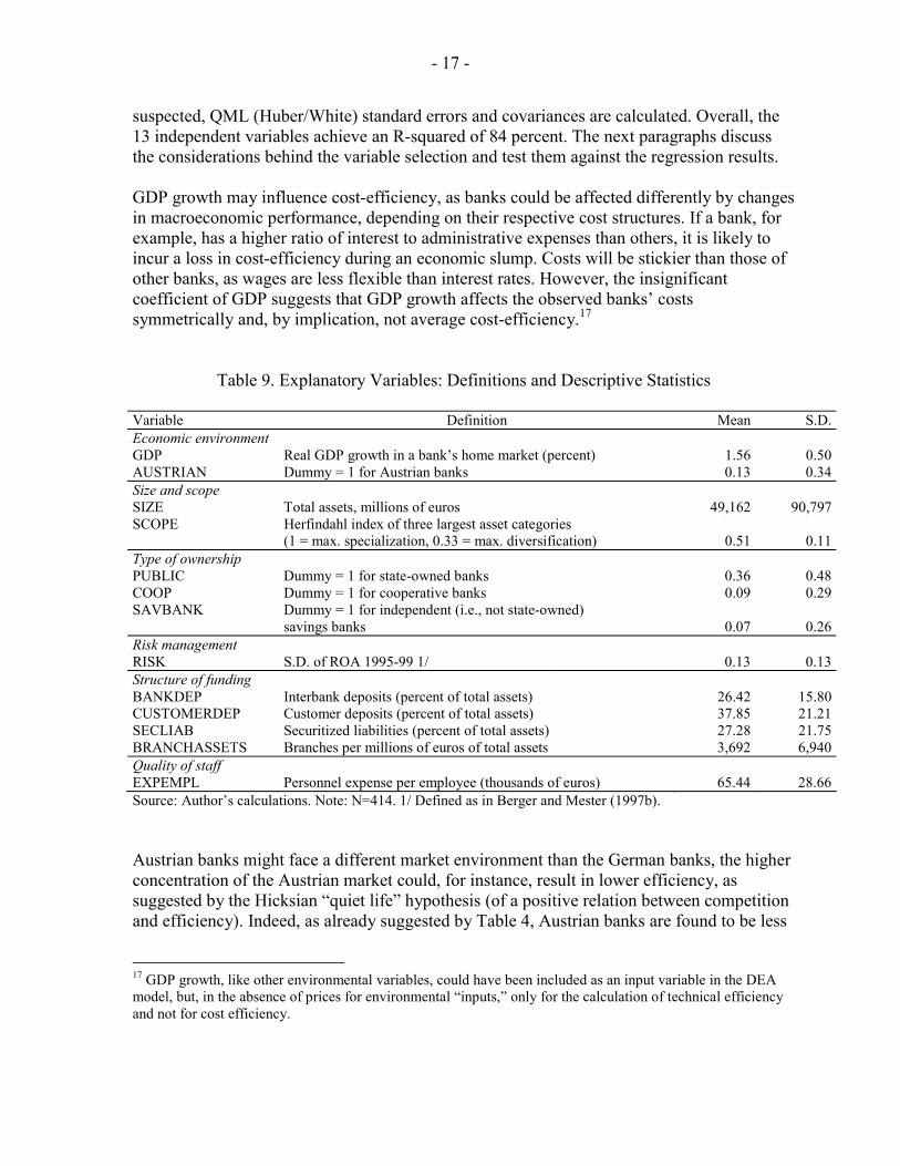
In order to explain differences in cost efficiency among the sample banks, the cost-efficiency scores are pooled over all five years and are regressed on a number of explanatory variables. Definitions and descriptive statistics of the explanatory variables included are shown in Table 9, the regression results in Table 10. As the scores are bounded between zero and unity, the use of a limited dependent variable (Tobit) model is required. As heteroscedasticity may be

16 As discussed in Section III, productivity change is defined as the mathematical product of the changes in cost efficiency, scale efficiency, and technology. Slight deviations from this identity in the tables are due to rounding.

- 17 -

suspected, QML (Huber/White) standard errors and covariances are calculated. Overall, the 13 independent variables achieve an R-squared of 84 percent. The next paragraphs discuss the considerations behind the variable selection and test them against the regression results. GDP growth may influence cost-efficiency, as banks could be affected differently by changes in macroeconomic performance, depending on their respective cost structures. If a bank, for example, has a higher ratio of interest to administrative expenses than others, it is likely to incur a loss in cost-efficiency during an economic slump. Costs will be stickier than those of other banks, as wages are less flexible than interest rates. However, the insignificant coefficient of GDP suggests that GDP growth affects the observed banks’ costs symmetrically and, by implication, not average cost-efficiency.17

Table 9. Explanatory Variables: Definitions and Descriptive Statistics

Variable Definition Mean S.D.Economic environment GDP Real GDP growth in a bank’s home market (percent) 1.56 0.50AUSTRIAN Dummy = 1 for Austrian banks 0.13 0.34Size and scope SIZE Total assets, millions of euros 49,162 90,797SCOPE Herfindahl index of three largest asset categories

(1 = max. specialization, 0.33 = max. diversification) 0.51 0.11Type of ownership PUBLIC Dummy = 1 for state-owned banks 0.36 0.48COOP Dummy = 1 for cooperative banks 0.09 0.29SAVBANK Dummy = 1 for independent (i.e., not state-owned)

savings banks 0.07 0.26Risk management RISK S.D. of ROA 1995-99 1/ 0.13 0.13Structure of funding BANKDEP Interbank deposits (percent of total assets) 26.42 15.80CUSTOMERDEP Customer deposits (percent of total assets) 37.85 21.21SECLIAB Securitized liabilities (percent of total assets) 27.28 21.75BRANCHASSETS Branches per millions of euros of total assets 3,692 6,940Quality of staff EXPEMPL Personnel expense per employee (thousands of euros) 65.44 28.66Source: Author’s calculations. Note: N=414. 1/ Defined as in Berger and Mester (1997b). Austrian banks might face a different market environment than the German banks, the higher concentration of the Austrian market could, for instance, result in lower efficiency, as suggested by the Hicksian “quiet life” hypothesis (of a positive relation between competition and efficiency). Indeed, as already suggested by Table 4, Austrian banks are found to be less

17 GDP growth, like other environmental variables, could have been included as an input variable in the DEA model, but, in the absence of prices for environmental “inputs,” only for the calculation of technical efficiency and not for cost efficiency.

- 18 -

cost-efficient than their German counterparts, the coefficient of the dummy AUSTRIAN being negative and significant at the 1 percent level. Size could have a positive impact on cost-efficiency via two channels: First, if it relates positively to market power, larger banks should pay less for their inputs. Second, there might be increasing returns to scale, i.e., input/output ratios could decline with increasing firm size. Increasing returns to scale could stem from fixed costs, e.g., for research or risk management, or from efficiency gains from a higher specialized workforce. Efficiencies of scope (increasing returns to output diversification), in turn, could, e.g., stem from the use of one input in the production of various outputs. Indeed, the coefficient of SIZE is positive and significant at the 1 percent level.18 However, the coefficient of SCOPE, an indicator of output diversification, while significant at the 1 percent level, is negative. These results suggest that while endogenous and exogenous growth could raise cost-efficiency, increasing output diversification could in fact be detrimental to cost-efficiency.

Table 10. Regression Results—Factors Explaining Differences in Cost-Efficiency

Variable Coefficient Standard Error z-Statistic Probability GDP -0.000870 0.017962 -0.048459 0.9614** AUSTRIAN -0.113791 0.035863 -3.172920 0.0015** SIZE 9.67E-10 1.13E-10 8.565252 0.0000** SCOPE 0.347083 0.075332 4.607346 0.0000** PUBLIC 0.043821 0.022106 1.982293 0.0474** COOP 0.020517 0.026253 0.781516 0.4345 SAVBANK -0.081515 0.022441 -3.632395 0.0003** RISK -0.226234 0.062824 -3.601079 0.0003** BANKDEP 0.010061 0.001687 5.964616 0.0000** CUSTOMERDEP 0.001778 0.001678 1.059824 0.2892** SECLIAB 0.012922 0.001508 8.569817 0.0000** BRANCHASSETS 171.9927 227.1709 0.757107 0.4490** EXPEMPL 0.001075 0.000216 4.974917 0.0000** Source: Author’s calculations. Notes: R-squared=0.84. ** (*) significant at the 1 (5) percent level. Different types of ownership could translate into different managerial objective functions and thus into differences in cost-efficiency, which might be suspected to increase with the degree of profit orientation of the bank's owners. German and Austrian banks typically belong to one of four legally distinct types of ownership. The most prevalent types are private ownership

18 To test for a potentially U-shaped average cost curve, the regression was also performed with dummies for three groups split according to size. The results, however, supported the findings of the regression reported here. The fact that this result seems to be at odds with those presented in Table 6 again confirms that regression analysis is more conclusive that mere comparisons of efficiency score by sub-samples (see Section I).

- 19 -

and state ownership. Other types are cooperative banks or independent (i.e., not state-owned) savings banks.19 Interestingly, the regression coefficient of the dummy for publicly owned banks (PUBLIC) is positive and significant at the 5 percent level. This result suggests that the cost advantage from the state-owned banks’ favorable credit ratings more than compensates for potentially weaker profit orientation.20 Thus, multivariate regression analysis confirms a similar result that Altunbas, Evans, and Molyneux (2001) inferred from comparing the average efficiency scores of sectors. With respect to the other dummies, the coefficient of the dummy for cooperative banks (COOP) is not significant at common levels, that is, there seems to be no difference in cost-efficiency relative to the base case of private banks. The coefficient of the dummy for independent (i.e., not state-owned) savings banks (SAVBANK) is negative and significant at the 1 percent level—here in line with the argument in the paragraph above. A bank's handling of risk is included as a regressor (RISK), defined—following Berger and Mester (1997b)—by the volatility of a bank's return on assets (ROA). It is often argued that cost-efficiency should be negatively related to the risk incurred by a bank, as risk management creates administrative costs. The evidence here does not support this claim, as the coefficient of RISK is negative and significant at the 1 percent level, implying that banks that are bad managing their risks are also bad managing their costs. As the cost of funds varies by source, the structure of funding will influence cost-efficiency. It is not straightforward ex ante which source of funds would be the most cost-efficient, due to the complex input/output relationships mentioned in Section IV (most importantly that customer deposits are partly paid for in services and not in interest). In the regression, the coefficients of BANKDEP and SECLIAB are positive and significant at the 1 percent level, while the coefficients of CUSTOMERDEP and BRANCHASSETS are insignificant at usual levels. These findings suggest that more cost-efficient banks draw a larger part of their funds from interbank deposits and securitized liabilities, while the share of customer deposits in total liabilities and a large retail network to generate them are neutral relative to cost-efficiency. It might be worth noting at this point that the variables BANKDEP, CUSTOMERDEP, SECLIAB, and BRANCHASSETS should also pick up most of the potential bias arising from the inclusion of the Landesbanken in the sample. The Landesbanken have higher ratios of bank deposits plus securitized liabilities to customer deposits, and lower ratios of branches to assets than the large private banks.

19 The sample distribution of the types of ownership can be inferred from the mean of the respective variable in Table 9. Privately (mostly stock market-listed) banks are the base case.

20 This suspicion is confirmed by regressing the average interest paid by a bank on its funds on the dummy PUBLIC and an intercept. The coefficient on the dummy is negative and significant at the 1 percent level. The argument, however, does not fully apply to the public savings banks, as they largely rely on deposit funding.

- 20 -

Lastly, the quality of a bank's staff might influence cost-efficiency if output per employee increased at a rate disproportionate to staff compensation. Indeed, the coefficient of EXPEMPL, a proxy for the average qualification level of staff, is positive and significant at the 1 percent level. This result is worth being viewed in the context of Brunner and others’ (2003) finding that the underdevelopment of high valued-added activities is one of the reasons for the comparatively low profitability of German banks.

VII. CONCLUSIONS

This study has several implications for bank management and policymaking: First, over the five-year period studied here, neither cost-efficiency nor productivity improved, on average, despite the deregulation and the merger wave of the 1990s. As others have found (e.g., Mukherjee, Lay, and Miller, 2001 for the U.S. post-deregulation period), efficiency gains might need considerable time to materialize, and this would probably be even more true in stringently regulated labor markets, such as Germany’s and Austria’s, which limit the potential efficiency gains from consolidation in the short and medium terms. Second, Austrian banks were found to be significantly less cost-efficient than German banks. This suggests, by implication from Hicks’s “quiet life” hypothesis, that the Austrian market is less competitive than the German market. Third, although there appear to be significantly increasing returns to scale, returns to scope are found to be negative in the German and Austrian banking systems. Thus, from a cost-efficiency point of view, there is clearly a rationale for mergers and acquisitions, at least among institutions with similar product portfolios. Fourth, no significant differences between the cost-efficiency of privately owned banks and cooperative banks were found. Independent (i.e., not state-owned) saving banks, however, were found to be significantly less cost-efficient on average, in line with the argument that they pursue other objectives in addition to profit. State-owned banks, in turn, were found to be, on average, more cost-efficient than other banks, which can probably be largely attributed to state guarantees that give them access to cheaper funds. Fifth, the study sheds light on the question of whether lower average interest rates on customer deposits than on other funds would justify the cost of running an extensive retail network. The evidence presented here would support a further shift of funding toward interbank deposits and securitized liabilities (from the perspective of an individual bank). Some limitations of the study should be noted. First, the study does not rest on a universally accepted model of the production process of a bank (simply because there is none). Second, an analogous critique applies to DEA, even though it is about as common as parametric approaches to measuring banks’ productivity. Future studies could investigate the effects of further market deregulation, increasing cross-border competition within the EU, mergers and acquisitions, and the removal of (formal) state guarantees.

- 21 -

REFERENCES

Alam, Ila M. Semenick, 2001, “A Nonparametric Approach for Assessing Productivity Dynamics of Large U.S. banks,” Journal of Money, Credit and Banking, Vol. 33 (No. 1), pp. 121–39.

Allen, Linda, and Anoop Rai, 1996‚ ”Operational Efficiency in Banking: An International Comparison,” Journal of Banking and Finance, Vol. 20 (No. 4), pp. 655–72.

Altunbas, Yener, Lynne Evans, and Philip Molyneux, 1997, “Universal Banks, Ownership and Efficiency: A Stochastic Frontier Analysis of the German Banking Market,” in The Recent Evolution of Financial Systems, ed. by Jack Levell (New York: St. Martin's Press; London: Macmillan Press).

———, 2001, “Bank Ownership and Efficiency,” Journal of Money, Credit and Banking, Vol. 33 (No. 4), pp. 926–54.

Berg, Sigbjorn Atle, Finn R. Forsund, and Eilev S. Jansen, 1992, “Malmquist Indices of Productivity Growth during the Deregulation of Norwegian Banking, 1980–89,” Scandinavian Journal of Economics, Vol. 94 (Supplement), pp. S211–28.

Berger, Allen N., and Timothy H. Hannan, 1998, “The Efficiency Cost of Market Power in the Banking Industry: A Test of the ‘Quiet Life’ and Related Hypotheses”, Review of Economics and Statistics, Vol. 80 (No. 3), pp. 454–65.

Berger, Allen N., and David B. Humphrey, 1991‚ “The Dominance of Inefficiencies over Scale and Product Mix Economies in Banking,” Journal of Monetary Economics, Vol. 28 (No. 1), pp. 117–48.

———, 1997‚ “Efficiency of Financial Institutions: International Survey and Directions for Future Research,” European Journal of Operational Research, Vol. 98 (No. 2), pp. 175–212.

Berger, Allen N., William C. Hunter, and Stephen G. Timme, 1993‚ “The Efficiency of Financial Institutions: A Review and Preview of Research: Past, Present, and Future,” Journal of Banking and Finance, Vol. 17 (No. 2-3), pp. 221–49.

Berger, Allen N., and Loretta J. Mester, 1997a, “Inside the Black Box: What Explains Differences in the Efficiencies of Financial institutions?,” Journal of Banking and Finance, Vol. 21 (No. 7), pp. 895–947.

———, 1997b, “Efficiency and Productivity Change in the U.S. Commercial Banking Industry: A Comparison of the 1980s and 1990s,” Federal Reserve Bank of Philadelphia Research Working Paper 97/05 (Philadelphia: Federal Reserve Bank of Philadelphia).

Brunner, Allan, Jörg Decressin, Daniel Hardy, and Beata Kudela, 2003, “Banking on Three Pillars in Europe: A Cross-Country Perspective on Germany,” in Germany: Selected Issues, IMF Staff Country Report No. 03/342 (Washington: International Monetary Fund).

- 22 -

Coelli, Tim, 1996, “A Guide to DEAP Version 2.1: A Data Envelopment Analysis (Computer) Program,” Center for Efficiency and Productivity Analysis Working Paper 96/08 (Armidale, New England: University of New England).

Debreu, Gérard, 1951, “The Coefficient of Resource Utilization,” Econometrica, Vol. 19, No. 3 (July), pp. 273–92.

Färe, Rolf, Shawna Grosskopf, and C. A. Knox Lovell, 1985, The Measurement of Efficiency of Production (Boston: Kluwer-Nijhoff Publishing).

———, 1994, Production Frontiers (Cambridge: Cambridge University Press).

Farrell, M.J., 1957, “The Measurement of Productive Efficiency,” Journal of the Royal Statistical Society, pp. 253–81.

Favero, Carlo A., and Luca Papi, 1995, “Technical Efficiency and Scale Efficiency in the Italian Banking Sector: A Non-Parametric Approach,” Applied Economics, Vol. 27 (No. 4), pp. 385–95.

Fixler, Dennis J. and Kimberly D. Zieschang, 1993, “An Index Number Approach to Measuring Bank Efficiency: An Application to Mergers,” Journal of Banking and Finance, Vol. 17 (April), pp. 437–50.

Grifell-Tatjé, Emili, and C. A. Knox Lovell, 1997, “The sources of productivity change in Spanish banking,” European Journal of Operational Research, Vol. 98 (No. 2), pp. 364–80.

International Monetary Fund, 2003, Germany: Financial System Stability Assessment, including Reports on the Observance of Standards and Codes on the Following Topics: Banking Supervision, Securities Regulation, Insurance Regulation, Monetary and Financial Policy Transparency, Payment Systems, and Securities Settlement, IMF Staff Country Report No. 03/343 (Washington: International Monetary Fund).

Koopmans, Tjalling Charles, 1951, “An Analysis of Production as an Efficient Combination of Activities,” in Activity Analysis of Production and Allocation, ed. by Tjalling Charles Koopmans (New York: Wiley).

Lang, Günter, and Peter Welzel, 1996‚ “Efficiency and Technical Progress in Banking: Empirical Results for a Panel of German Cooperative Banks,” Journal of Banking and Finance, Vo. 20 (No. 6), pp. 1003–23.

Lovell, C. A. Knox, 1993, “Production Frontiers and Productive Efficiency,” in The measurement of productive efficiency: Techniques and applications, ed. by Harold O. Fried, C. A. Knox Lovell, and Shelton S. Schmidt (Oxford: Oxford University Press).

Malmquist, S., 1953, “Index numbers and indifference surfaces,” Trabajos de Estadística, pp. 209–232.

- 23 -

Maudos, Joaquin and José M. Pastor, 2003, “Cost and Profit Efficiency in the Spanish Banking Sector (1985-1996): A Non-Parametric Approach,” Applied Financial Economics, Vol. 13 (No. 1), pp. 1–12.

Mukherjee, Kankana, Subhash C. Ray, and Stephen M. Miller, 2001, “Productivity Growth in Large U.S. Commercial Banks: The Initial Post-Deregulation Experience,” Journal of Banking and Finance, Vol. 25 (No. 5) pp. 913–39.

Pastor, José Manuel, 2002, “Credit Risk and Efficiency in the European Banking System: A Three-Stage Analysis”, Applied Financial Economics, Vol. 12 (No. 12), pp. 895–911.

———, Francisco Pérez, and Javier Quesada, 1997, “Efficiency Analysis in Banking Firms: An International Comparison,” European Journal of Operational Research, Vol. 98 (No. 2), pp. 395–407.

Peristiani, Stavros, 1996, “Do Mergers Improve the X-Efficiency and Scale Efficiency of U.S. Banks? Evidence from the 1980s,” Journal of Money, Credit, and Banking, Vol. 29 (No. 3), pp. 326–37.

Resti, Andrea, 1997, “Evaluating the Cost-Efficiency of the Italian Banking System: What Can Be Learnt from the Joint Application of Parametric and Non-Parametric Techniques,” Journal of Banking and Finance, Vol. 21 (No. 2), pp. 221–50.

Sealey, Calvin W., Jr., and James T. Lindley, 1977, “Inputs, Outputs, and a Theory of Production and Cost at Depository Financial Institutions,” Journal of Finance, Vol. 32 (No. 4), pp. 1251–66.

Seiford, Lawrence M., and Robert M. Thrall, 1990, “Recent Developments in DEA: The Mathematical Programming Approach to Frontier Analysis ,” Journal of Econometrics, Vol. 46 (Nos. 1–2), pp. 7–38.

Sheldon, George, 1994, “Nichtparametrische Messung des technischen Fortschritts im Schweizer Bankensektor,” Swiss Journal of Economics and Statistics, Vol. 130 (No. 4), pp. 691–707.

Shephard, Ronald W., 1970, Theory of Cost and Production Functions (Princeton, New Jersey: Princeton University Press).

Vennet, Rudi Vander, 2002, Cost and Profit Efficiency of Financial Conglomerates and Universal Banks in Europe, Journal of Money, Credit and Banking, Vol. 34 (No. 1), pp. 254–82.