experimental procedures and data analysis of orthotropic … · experimental procedures and data...
TRANSCRIPT

Experimental Procedures and Data Analysis of Orthotropic Composites
by
Nathan Schmidt
A Thesis Presented in Partial Fulfillment
of the Requirements for the Degree
Master of Science
Approved August 2016 by the
Graduate Supervisory Committee:
Subramaniam Rajan, Chair
Narayanan Neithalath
Barzin Mobasher
ARIZONA STATE UNIVERSITY
December 2016

i
ABSTRACT
Composite materials are widely used in various structural applications, including
within the automotive and aerospace industries. Unidirectional composite layups have
replaced other materials such as metals due to composites’ high strength-to-weight ratio
and durability. Finite-element (FE) models are actively being developed to model
response of composite systems subjected to a variety of loads including impact loads.
These FE models rely on an array of measured material properties as input for accuracy.
This work focuses on an orthotropic plasticity constitutive model that has three
components – deformation, damage and failure. The model relies on the material
properties of the composite such as Young’s modulus, Poisson’s ratio, stress-strain
curves in the principal and off-axis material directions, etc. This thesis focuses on two
areas important to the development of the FE model – tabbing of the test specimens and
data processing of the tests used to generate the required stress-strain curves. A
comparative study has been performed on three candidate adhesives using double lap-
shear testing to determine their effectiveness in composite specimen tabbing. These tests
determined the 3M DP460 epoxy performs best in shear. The Loctite Superglue with 80%
the ultimate stress of the 3M DP460 epoxy is acceptable when test specimens have to be
ready for testing within a few hours. JB KwikWeld is not suitable for tabbing. In
addition, the Experimental Data Processing (EDP) program has been improved for use in
post-processing raw data from composites test. EDP has improved to allow for complete
processing with the implementation of new weighted least squares smoothing options,
curve averaging techniques, and new functionality for data manipulation.

ii
ACKNOWLEDGMENTS
I would like to thank my advisor Dr. Rajan for his help and support during my
time here. I would also like to thank my committee members Dr. Neithalath and Dr.
Mobasher for their teaching. Finally, I would like to thank Canio Hoffarth and Bilal
Khaled for their help in experimentation.

iii
TABLE OF CONTENTS
Page
LIST OF TABLES ............................................................................................................. vi
LIST OF FIGURES .......................................................................................................... vii
CHAPTER
1 INTRODUCTION ........................................................................................................... 1
1.1 Literature Review ..................................................................................................... 1
1.2 Thesis Objectives ...................................................................................................... 3
2 EXPERIMENTAL PROCEDURES ................................................................................ 5
2.1 Experimental Procedures for Orthotropic Composites ............................................. 5
2.1.1 Material Data ..................................................................................................... 5
2.1.2 Test Equipment .................................................................................................. 6
2.1.3 Force Data Collection ........................................................................................ 7
2.1.4 Strain Data Collection ........................................................................................ 7
2.1.5 Summary of Raw Data ....................................................................................... 8
2.2 Experimental Procedures for Adhesives ................................................................... 9
2.2.1 Double Lap-Shear Test Plan .............................................................................. 9
2.2.2 Post-Processing ................................................................................................ 19
2.2.3 Results .............................................................................................................. 23
3 EXPERIMENTAL DATA PROCESSING SOFTWARE DEVELOPMENT .............. 28

iv
CHAPTER Page
3.1 Overview ................................................................................................................. 28
3.2 Processing Steps ..................................................................................................... 29
3.2.1 Step 1. Read Raw Data .................................................................................... 29
3.2.2 Step 2. Data Processing.................................................................................... 30
3.2.3 Step 3. Smoothing ............................................................................................ 30
3.2.4 Step 4. Plotting Stress-Strain Curves ............................................................... 31
3.2.5 Step 5. Generating the Model Curve................................................................ 31
3.3 Implementation ....................................................................................................... 32
3.3.1 Curve Averaging .............................................................................................. 32
3.3.2 Lowess/Loess Theory ...................................................................................... 33
3.3.3 Lowess Algorithm ............................................................................................ 34
3.3.4 Robust Local Regression Theory ..................................................................... 36
3.3.5 Robust Lowess Algorithm ............................................................................... 37
3.3.6 Comparison of Smoothing Strategies .............................................................. 38
4 POST-PROCESSING TO GENERATE INPUT FOR CONSTITUTIVE MODEL ..... 62
5 CONCLUSIONS............................................................................................................ 83
5.1 Future Work ............................................................................................................ 84
REFERENCES ................................................................................................................. 85

v
APPENDIX Page
A LOWESS EXAMPLE ........................................................................................... 87
B ROBUST LOWESS EXAMPLE .......................................................................... 94
C EDP GENERATED MODEL CURVES FOR T800/F3900 COMPOSITE ....... 101

vi
LIST OF TABLES
Table Page
1. Adhesive Data ......................................................................................................... 9
2. Adhesive Shear Strength Summary ...................................................................... 10
3. Bond Data ............................................................................................................. 14
4. Preparation Instructions for Aadhesive 1: 3M DP460 .......................................... 14
5. Preparation Instructions for Adhesive 2. Loctite Super Glue ............................... 15
6. Preparation Instructions for Adhesive 3. J-B Weld KwikWeld ............................ 15
7. Load Data Summary Table for Fiberglass-on-Fiberglass Specimens................... 23
8. Functions for Editing Data. ................................................................................... 71
9. Fitting Types and Their Descriptions ................................................................... 75
10. Smoothing Methods and Brief Descriptions. ........................................................ 75
11. Lowess Example Data........................................................................................... 88
12. Smoothed Lowess Example Data and Residual Data. .......................................... 92
13. Robust Lowess Example Data. The Original Data and Corresponding Residuals
from a Single Iteration of Lowess Smoothing are Shown. ................................... 95
14. Smoothened Lowess Example Data...................................................................... 98

vii
LIST OF FIGURES
Figure Page
1. Photos of Test Equipment Used in Composites Testing. MTS Load Frame (Left)
and Point Grey Grasshopper 3 Camera Set Up (Right) .......................................... 6
2. Photos of G10 Fiberglass Specimen Components. The Top 2.44 mm Piece (Left).
The Bottom 2.44 mm Spacer (Center). One 1.52 mm Piece for the Bottom
(Right). .................................................................................................................. 11
3. Complete Substrate Surface Preparation Example. .............................................. 12
4. Adhered 3ME Specimens with Front View (Left) and Side View (Right)........... 12
5. Adhered JBQ Specimen with Front View (Left) and Side View (Right). ............ 13
6. Assembly of Adhesive Test Specimen. (A) Initial Set Up of First Piece and 1.52
mm Spacer. (B) Placing the 2.44 Mm Top Piece and Bottom Spacer. (C) Placing
the Final 1.52 mm Piece........................................................................................ 13
7. Form, Dimension, and Nomenclature of Individual Test Specimen (All
Measurements in mm)........................................................................................... 17
8. DIC Image Of The Full 3ME-1 Specimen During Testing. ................................. 18
9. Front View (Left) And Side View (Right) Of Shear Testing Setup. .................... 19
10. Normal (Eyy) Strain Field (Left), Shear (Exy) Strain Field (Center) and Z Position
for Specimen 3ME-1 Just Before Failure. ............................................................ 21
11. Displacement Plot for Specimen 3ME-1 Just Before Failure. .............................. 22
12. Stress-Strain Plot for 3M DP460 Showing All 4 Acceptable Tests. .................... 23

viii
Figure Page
13. Specimen Photos of Gage Region for 3M DP460 Epoxy (3ME). (A) Back Side of
3ME-4 and (B) Left Side of 3ME-2 Prior to Testing. (C) Back Side of 3ME-2
After Testing. ........................................................................................................ 24
14. Specimen Photos of Gage Region for Loctite Superglue (LSG). (A) Back Side
and (B) Left Side of LSG-4 Before Testing. (C) Back Side Surface of LSG-4
After Testing. ........................................................................................................ 25
15. Specimen Photos of Gage Region for JB Kwik Kwikweld (JBQ). (A) Back Side
of Specimen JBQ-3 Before Testing. (B) Right Side of Specimen JBQ-2 Before
Testing. (C) Back Side of JBQ-3 After Testing. (D) Front Side of JBQ-3 After
Testing. (E) Left Side of JBQ-2 After Testing. .................................................... 27
16. Raw Strain Data from 3-Direction Compression Test (Case 1). .......................... 39
17. Raw Stress Data from 3-Direction Compression Test (Case 2). .......................... 40
18. Raw Engineering Strain Data from 2-3 Plane Shear Test (Case 3). ..................... 41
19. Raw Stress Data from 1-3 Plane Shear Test (Case 4). .......................................... 42
20. Moving Median Filter. Case 1 (Top) and Case 2 (Bottom) .................................. 43
21. Case 3 Smoothened with Moving Median Filter. Full Plot (Top) and Zoomed Plot
(Bottom). ............................................................................................................... 45
22. Case 4 Smoothened with Moving Median Filter Using 3 Points (Top) and 25
Points (Bottom). .................................................................................................... 47
23. Case 1 with SMA (Top) and PMA (Bottom) Zoomed to First 100 Seconds. ....... 49
24. Case 2 Smoothened with SMA (Top) and PMA (Bottom) Zoomed to First 50
Seconds. ................................................................................................................ 51

ix
Figure Page
25. Case 3 Smoothed with SMA (Top) and PMA (Bottom) Methods........................ 53
26. Case 4 Smoothened with SMA (Left) and PMA (Right) Using 15 Points and 2
Iterations Zoomed to Initial 125 Seconds. ............................................................ 55
27. Case 1 Smoothed with Lowess (Red) and Loess (Green) Methods Zoomed to the
First 100 Seconds .................................................................................................. 57
28. Case 2 Smoothened With Lowess (Red) and Loess (Green) Methods Zoomed to
the First 50 Seconds With 11 Points (Top) and 15 Points (Bottom) .................... 58
29. Case 3 Smoothed with Lowess Method. ............................................................... 59
30. Case 4 Smoothened with Lowess (Red) and Loess (Green) Methods Zoomed in to
Show Local Outliers ............................................................................................. 60
31. Case 3 Smoothened with Robust Lowess (Red) and Robust Loess (Green)
Methods................................................................................................................. 61
32. Case 4 Smoothened with Robust Lowess (Red) Compared to Lowess (Green). .. 62
33. Step 1 of Processing Involves Reading in the Raw Data. The Read Raw Data
Button (Highlighted in Red) Is Found at the Top of the Screen in the Tool Bar. . 63
34. The Read Raw Data Interface. In Here, Multiple Sets of Data May Be Read in at
Once Before Closing The Interface. ..................................................................... 64
35. The Read Raw Data Interface with DIC Information Entered. ............................ 66
36. Read Raw Data Dialogue with MTS Data Entered. ............................................. 67
37. Plot Toggle Area in Top Left of View Screen. ..................................................... 68
38. Raw Data Plotted in EDP. ..................................................................................... 69
39. Location of Edit or View Data Button .................................................................. 70

x
40. Edit Raw Data & View Smoothened and Fitted Data Interface Upon Launch. ... 71
41. Interface with Process Data Button Highlighted .................................................. 73
42. Data Set-Zone Data Dialogue Box ....................................................................... 74
43. Smoothened Data Generated with Lowess Smoothing Plotted in EDP ................ 76
44. Smoothened Data Generated with SMA Method Plotted in EDP ........................ 77
45. Stress-Strain Curves for the Four Replicates Plotted in EDP ............................... 78
46. Interface with Best Fit Plot Button Highlighted. .................................................. 79
47. Best Fit input Dialogue Box ................................................................................. 80
48. Interface with Edit Graph Settings Button Highlighted ........................................ 80
49. XY Graph Data Interface with The Graph Attributes Tab (Left) and Graph Layout
Tab (Right) Shown ................................................................................................ 81
50. Final Model Curve for TFT2 Generated with Lowess (Blue) and SMA (Grey)
Smoothing Methods Plotted in EDP ..................................................................... 82
51. Lowess Example Data and Smoothed Data Plots. ................................................ 92
52. Example Data With Smoothed Data Generated with Loess Method. ................... 93
53. Robust Lowess Example Raw Data and Smoothened Data Plots ......................... 99
54. Smoothing Example Data with Smoothed Data from Robust Loess Method. ... 100
55. 1-Direction Compression Model Curve .............................................................. 102
56. 2-Direction Compression Model Curve .............................................................. 102
57. 3-Direction Compression Model Curve .............................................................. 103
58. 1-3 Off-Axis Compression Model Curve ........................................................... 103
59. 2-3 Off-Axis Compression Model Curve ........................................................... 104
60. 1-2 Shear Model Curve ....................................................................................... 104

xi
61. 1-3 Shear Model Curve ....................................................................................... 105
62. 2-3 Shear Model Curve ....................................................................................... 105
63. 1-Direction Tension Model Curve ...................................................................... 106
64. 2-Direction Tension Model Curve ...................................................................... 106
65. 3-Direction Tension Model Curve ...................................................................... 107
66. Off-Axis Tension Model Curve .......................................................................... 107

1
1 Introduction
Composite materials are widely used in various structural applications, including
within the automotive and aerospace industries. Unidirectional composite layups have
replaced other materials such as metals due to composites’ high strength-to-weight ratio
and durability. Finite-element (FE) models are actively being developed to model
response of composite systems subjected to a variety of loads including impact loads.
These FE models rely on an array of measured material properties as input for accuracy.
This work focuses on a constitutive model implemented in LS-DYNA® called MAT213,
an orthotropic plasticity model that has three components – deformation, damage and
failure (Livermore Software Technology Corporation (LSTC) 2015); (Goldberg, et al.
2015); (Harrington, et al. 2016). The model relies on the material properties of the
composite such as Young’s modulus, Poisson’s ratio, stress-strain curves in the principal
and off-axis material directions, etc.
1.1 Literature Review
This thesis has two major areas of focus related to the characterization of
orthotropic composites: (1) sample preparation with focus on tabbing of the specimens to
enable proper gripping and response of the specimen in the grips, and (2) development of
a graphical-user interface (GUI)-based computer program for processing the
experimental results from the material characterization tests.
Tabbing strategies for composite testing have been explored in the past with
several tabbing guides available for use in composites testing (Adams and Adams 2002).
Since tabs are attached to the test specimens via adhesives, studies of adhesives are often

2
done as comparison studies between adhesives. Research in the area of adhesives has
found that symmetric lap-shear testing is best for characterizing adhesives because the
response from this test closely matches the expected true shear response (Renton 1976).
In their analysis of several papers, Matthews et al. found primary characteristics
necessary in adhesives in shear includes adherend type, overlap size, and low shear
modulus, among others. Adhesives testing using isotropic materials such as metals
simplifies the analysis by reducing the number of failure modes in test specimens.
Anisotropy in composites introduces not only failure modes within the substrate but new
interactions between the adhesive and substrate. Failure in the interface between substrate
adhesives in any application have commonly been attributed to quality control problems,
however (Matthews, Kilty and Godwin 1982). Yang and co-workers developed an
analytical FE model of ASTM lap shear specimens using equivalent plastic strain
criterion and the fracture mechanic approach for use in comparing adhesives (Yang,
Tomblin and Guan 2003).
There is a variety of smoothing methods available for removing outliers that
potentially show in raw data. Savitzky and Golay developed one of the early least-squares
polynomial filters, using local nonlinear regression to smooth data (Savitzky and Golay
1964). Cleveland in 1979 developed the basic assumptions used in the Locally Weighted
Regression and Smoothing Scatterplots (Lowess) method and its robust version,
including parameter selection and weight function determination. An improvement from
other least-squares smoothing techniques, Lowess and the related Local Regression
(Loess) smoothing method use a local regression weighted based on the proximity and –
for robustness and removing outliers – the residuals of each data point within the local

3
region (Cleveland 1979). Other filters may include those based on power law,
logarithmic, and exponential equations (Stroud 1999).
1.2 Thesis Objectives
This thesis focuses on two areas important to the development of the MAT213 FE
model – tabbing of the test specimens and data processing of the tests used to generate
the required stress-strain curves. The material chosen for validating MAT213 is the
T800S/3900-2B unidirectional composite manufactured by Toray.
Tabbing: Some tabbing strategies for use in characterizing composites have been
followed in characterizing the T800S/3900-2B composite at Arizona State University as
previously described (Adams and Adams 2002). During this preliminary testing, G-10
glass fabric/epoxy (fiberglass) tabs sometimes de-bonded from the T800S/3900-2B
substrate. This failure is in the adhesive rather than in either the fiberglass or the
T800S/3900-2B substrate. Three candidate adhesives were selected for testing to
determine which is best suited for use with composite tabbing: 3M DP460 – the original
adhesive used, Loctite Super Glue, and J-B KwikWeld (3M 2015), (Henkel 2014), (J-B
Weld It Australia 2012). All adhesives selected are paste adhesives that are easy to use
during sample preparation. To test each adhesive, standard test procedures for double lap
shear adhesive characterization tests is used (ASTM, 2008). Supplemental analysis using
Digital Image Correlation (DIC) during these tests is also used to ensure consistent
results between tests.
Data Processing: To simplify the process of reviewing experimental raw data and
generating material constants and stress-strain curves, a program has been developed at

4
Arizona State University called Experimental Data Processing (EDP) program (Vokshi
2011). The current version of EDP has the following functionalities.
(1) Reading raw data from text file (*.txt) and comma separated file (*.csv) with
several different field delimiters. Displaying the data as x-y plot.
(2) Displaying and editing raw data in the form of a spreadsheet.
(3) Identifying outliers using Chauvenet algorithm (Lin and Sherman 2007).
(4) Smoothing the raw data using the following options – median, simple moving
average, polynomial moving average, Loess, robust Loess, Lowess, and robust
Lowess. The smoothened data can then be used to create a stress-strain curve.
(5) Fitting curves to the smoothened data using the following fitting equations –
linear polynomial, quadratic polynomial, cubic polynomail, quartic polynomial,
qunitic polynomial, exponential function of the form bxae , logarithmic function
of the form loga bx and power equation of the form bax .
(6) Creating a single stress-strain curve from the stress-strain curves processed from
several replicates using a least-squares fit model.
(7) Creating the MAT213 constitutive model data for LS-DYNA analysis.
(8) Carrying out distribution analysis of experimental data using 2-parameter
Weibull, 3-parameter Weibull, normal, log normal, Gamma and generalized
exponential distribution models.
In this thesis, the focus is on items (1)-(6). Existing functionalities were enhanced and
new functionalities were added.

5
2 Experimental Procedures
Building finite element models of composites requires material properties such as
modulus of elasticity, Poisson’s ratio, etc. or the entire stress-strain curve. These material
property values are usually obtained from laboratory experiments. The typical pre-test
steps are as follows.
Step 1. Identify the appropriate ASTM document governing the test for the
selected material. This will help identify the test machine; the grips to be used; the
test conditions such as loading rate, temperature etc.; how test data will be
obtained in real time; and how the test data will be processed after the test to
obtain the material properties.
Step 2. Generate the dimensions for a typical specimen. Machine the specimen.
Step 3. Identify how the specimen is inserted and held in the grips.
Step 4. Prepare the specimen for test – if required, bonding the tabs to the
specimen, or bonding the specimen to the test fixture, and speckling the specimen.
In this chapter, the test methods for characterizing unidirectional composites are
discussed and candidate adhesives that can be used in preparing the composite test
specimens are investigated with the test results are discussed.
2.1 Experimental Procedures for Orthotropic Composites
This section covers the methods used to gather data to characterize the
T800S/3900-2B composite for use with MAT 213.
2.1.1 Material Data
The T800S/3900-2B composite manufactured by Toray Carbon Fibers America,
Inc. is a unidirectional fiber/epoxy resin composite material. Characterization testing is

6
done with three different panel types of varying thickness to create specimens. The T800
composite has a tensile strength of 430 ksi (2950 MPa) (Toray Carbon Fibers America,
Inc. n.d.)
2.1.2 Test Equipment
Data is collected using a MTS 810 Load Frame and Two Point Grey
Grasshopper® 3 cameras. The details of the testing system are written in reference to
testing at quasi-static and room temperature conditions.
Figure 1. Photos of test equipment used in composites testing. MTS Load Frame (left)
and Point Grey Grasshopper 3 camera set up (right)
Test Frame
The MTS 810 Load Frame has a 10 inch stroke and a 20 kip compression and
tension capacity. The frame features interchangeable grips for testing different specimen
types. The system is controlled by a MTS FlexTest® digital controller. The digital
interface allows for load or stroke controlled load testing. Force and displacement data is
collected every second.

7
Digital Image Correlation (DIC) Equipment
The Point Grey Grasshopper® 3 5.0 Megapixel cameras feature mono coloring, 15
max frames per second, and a digital interface. Cameras are calibrated using VIC3D 7©
software (Correlated Solutions 2014). The resulting images from testing are then
analyzed in VIC3D 7©.
2.1.3 Force Data Collection
Force data is collected from the MTS system once per second during testing and
is stored in a .dat file. The test is actuator controlled, with the test speed defined as
distance per minute. The test speed varies based on the test being done. Once collected,
the force data is converted to stress by using the cross-sectional area of the testing region
measured before testing. For each test, the thickness/width measurements are taken at 8-
12 points in the area of interest.
2.1.4 Strain Data Collection
The DIC system relies on two cameras capturing images of the speckled specimen
during quasi-static testing. DIC relies on smooth surfaces with few rapid changes in
geometry. Speckling involves painting the entire surface of the testing region white, then
applying a random pattern of black spots. While there are many methods to apply random
speckling patterns, small specimens such as those used to characterize the T800S/3900-
2B composite are painted using a fine mist of black paint.
Prior to each test, calibration must be done to ensure the VIC3D 7© software is
able to accurately pick up on and quantify relative displacements. Pictures are taken over
an interval varying from 3 to 10 second, depending on the quasi-static experiment being
done. For example, a relatively quick test such as a 2-3 direction Iosipescu shear test

8
takes one picture every 3 seconds; a longer test such as any off-axis compression test,
which lasts approximately 15 minutes, involves one picture every 10 seconds.
The calibration and speckle images taken before and during testing are then
analyzed using VIC3D 7© software. Within this program, the region of interest is selected
for analysis. Once analyzed, various strain fields and displacements can be plotted over a
2-dimensional image of the specimen over time. Only index values and corresponding
relevant strain values are necessary when exporting data in a Comma Separated Value
(CSV) file. For example, in a 1-direction tension test, longitudinal (eyy) strains are used.
In a 2-3 shear test, shear (exy) strains are used. If the area of interest is large enough or
stress concentrations are noticeable in certain regions, a new region may be defined to
collect localized information that may be more indicative of the true behavior of the
material.
2.1.5 Summary of Raw Data
Following testing, there are two files with unprocessed data that will be used to
create a characteristic curve for a material in one test. The DAT file has information on
the testing machine, basic testing information (including test name and length of time of
testing), and the data itself: the raw time in seconds, the relative displacement of the
loading head in inches, and the force value in pounds. The CSV file has just the raw data:
the indices, the relevant strains, and any additional data sets selected for export.
Both raw data files may require modification in the following cases: if the test was
stopped and resumed, the DAT file includes a new header at the stopping index; if either
test has empty lines mixed with data for any reason, those lines must be deleted.

9
2.2 Experimental Procedures for Adhesives
During preliminary testing of the T800/F3900 unidirectional composites, it was
found that parts of the test specimens in the grips were being crushed. Lowering the grip
pressure did not help since then the specimens tended to slip. To mitigate crushing,
fiberglass tabs are adhered to the specimens in the gripping regions. However, these
adhesives can potentially fail in shear during testing. A test plan was created to evaluate
candidate adhesives suitable for the composite tests described earlier. Specifically, double
lap shear tests are performed based on standards and recommendations outlined in ASTM
D3528-96 (ASTM, 2008).
2.2.1 Double Lap-Shear Test Plan
This subsection describes the test plan for the adhesive comparison study.
2.2.1.1 Adhesive Data
Three candidate adhesives were selected for evaluation based on prior experience
with testing composites at Arizona State University and Ohio State University. The
names and relevant data for the candidate adhesives are listed in Table 1.
Table 1. Adhesive Data
Adhesive
Name
Specimen
Code
Mfr. Type Form MFG
Date
Code #
3M
DP460
3ME 3M Epoxy Paste Resin:
MAY-18-
2015
Hardener:
MAY-28-
2015
7000000872
Loctite
Super
Glue
LSG Henkel Cyanoacrylate Liquid MAR-10-
2015
43072
KwikWeld JBQ J-B
Weld
Epoxy Paste APR-04-
2015
8276F

10
Preparation instructions for each adhesive including substrate surface preparation
procedure, mixing directions, application conditions, assembly conditions prior to
pressure, curing conditions, and conditioning procedure are presented in Section 2.2.1.3.
2.2.1.2 Substrate Data
The substrate refers to the material on which the adhesive is applied. Most
adhesives testing standards provide guidelines for using a metal substrate such as
aluminum (ASTM 2010, ASTM 2008). For the tests described in this report, in order to
best relate the results of these tests to application with unidirectional composites,
fiberglass (Acculam® Epoxyglas™ G10-FR4 manufactured by Accurate Plastics Inc,
NY) specimens are used. For these tests, the fiberglass is used as the only substrate
whose tensile strength is 275.79 MPa (1-direction) and 241.32 MPa (2-direction)
(Accurate Plastics, Inc. 2016). The tensile strength of this material exceeds that of the
three adhesives in the test plan (see Table 2).
Table 2. Adhesive Shear Strength Summary
Adhesive Substrate Maximum Shear Stress (MPa)
3M DP460 Phenolic 9.653
Aluminum 31.026
Loctite Super
Glue
Not Provided (lower limit) 9.997
Not Provided (upper limit) 19.995
JB Kwik Weld Not Provided 7.171
2.2.1.3 Adhesive Preparation
The adhesive preparation information is available from the manufacturer’s
technical sheets (3M 2015), (J-B Weld It Australia 2012), (Henkel 2014). The details of
the adhesive testing as performed are presented in Table 4 Table 5, and Table 6. All steps
and recommendations were followed verbatim.

11
Materials Used and Terminology
This section details the tools and terminology referenced in the subsequent
sections on adhesive-specific procedures. Preparation is done at room temperature for all
adhesives. Each testing specimen is composed of several pieces adhered together. The
pieces used in sample creation are outlined in Figure 2.
Figure 2. Photos of G10 Fiberglass specimen components. The top 2.44 mm piece (left).
The bottom 2.44 mm spacer (center). One 1.52 mm piece for the bottom (right).
Step 1 is surface preparation. In all cases, this involves sanding the surface of the
specimen with 1000-grit sandpaper and removing the dust with a water based cleanser
(available from Micro Measurements, PA). The cleanser includes two parts: Conditioner

12
A, an acidic solution acting as both as etchant and cleanser, and Neutralizer 5A, an
ammonia-based solution to neutralize the acidic conditioner. Following step 1, the
surfaces of the bonding areas should appear as they do in Figure 3.
Figure 3. Complete substrate surface preparation example.
When applying the adhesive in step 3, special care should be taken to ensure the
adhesive has spread evenly over the entire adhered surface. After placing the two surfaces
together, the adhesive is visible beneath the fiberglass. As shown in Figure 4, the adhered
gage region has a darker appearance where the adhesive has set. In addition, Figure 5 also
shows the side view of an adhered specimen. While excess glue may be wiped away from
the edges, a small amount of adhesive on the edge is acceptable.
Figure 4. Adhered 3ME specimens with front view (left) and side view (right).

13
Figure 5. Adhered JBQ specimen with front view (left) and side view (right).
Step 4 involves assembly of the specimen. Photos of the assembly are shown in
Figure 6.
Figure 6. Assembly of adhesive test specimen. (A) Initial set up of first piece and 1.52
mm spacer. (B) Placing the 2.44 mm top piece and bottom spacer. (C) Placing the final
1.52 mm piece.
A
B
C

14
Complete bond information is summarized in Table 3.
Table 3. Bond Data
Adhesive Application
Method
Bonding
Method
Thickness
of Adhesive
Layer (mm)
Length of
Overlap
(mm)
Conditioning
Notes
3M DP460 Wooden
Applicator
No-added
pressure ~0.3
15
Store in dry
place at room-
temperature
until testing
Loctite
Super Glue
Long-neck
Nozzle
Manual
Pressure ~0.15
JB Kwik
Weld
Wooden
Applicator
No-added
pressure ~0.6
Adhesive 1. 3M DP460
Table 4. Preparation instructions for adhesive 1: 3M DP460
Surface
Preparation
Light sanding with 1000–grit sandpaper. All dust is then removed using
a water based cleaning solution.
Mixing DP460 is provided in a dual syringe plastic pack to be used with a
manufacturer designed applicator system. Enough pressure is applied to
the applicator on a surface designated for mixing to ensure even flow
from the two packs. A small quantity may need to be discarded before
the adhesive flows evenly. The two components are mixed by hand
using a wooden applicator until adhesive is of consistent appearance.
Application
Conditions
Adhesive is applied evenly in a thin layer over the bonding area using
the wooden applicator. Excess adhesive is removed from edges using
the applicator. Only one coat of adhesive is necessary.
Assembly
Conditions
Immediately after the adhesive is applied, the second surface is placed
on top with a 1.52 mm spacer on the opposing end to allow for even
adhesion. The adhesive is then applied on the third and fourth surfaces
with the second 1.52 mm piece being placed on top with the 2.44 mm
spacer. Because adhesive does not cure immediately, the two sides are
aligned as needed.
Curing
Conditions
Once the surfaces are aligned, no external pressure is applied on the
bond aside from the specimen’s own weight. As the material sets,
excess adhesive may be cleaned with tissue paper. The specimen is then
left in a dry location at room temperature for 48 hours to allow for
complete curing.
Conditioning
Procedure
The specimens are stored at room temperature between bonding and
testing. They are not to be exposed to heat or water.

15
Adhesive 2. Loctite Super Glue
Table 5. Preparation instructions for adhesive 2. Loctite Super Glue
Surface
Preparation
Light sanding with 1000–grit sandpaper. All dust is then removed using
a water based cleaning solution.
Mixing This step is not needed for this adhesive.
Application
Conditions
Application directions specify approximately one dot per square inch of
surface to be bonded. To ensure a complete surface bond for tests,
several drops of adhesive are placed in the center of the bonding area to
allow for applied pressure to spread the adhesive to the edges. Only one
coat is necessary.
Assembly
Conditions
Immediately after the adhesive is applied, the second surface is placed
on top.
Curing
Conditions
Once the surfaces are aligned, they are held together by hand for 15-30
seconds at room temperature to allow the bond to set. As the material
sets, excess adhesive may be cleaned with tissue paper. The procedure
is repeated for the spacer and the second 1.52 mm piece.
Conditioning
Procedure
The specimens are stored at room temperature between bonding and
testing. They are not to be exposed to heat or water.
Adhesive 3. J-B KwikWeld
Table 6. Preparation instructions for adhesive 3. J-B Weld KwikWeld
Surface
Preparation
Light sanding with 1000–grit sandpaper is performed first to clean
bonding surfaces. Remove all dust with a water based cleaning solution.
Mixing J-B Weld KwikWeld is provided two separate tubes: epoxy resin and
epoxy hardener. Equal parts of both tubes are squeezed onto a
disposable surface designated for mixing. The two components are
mixed by hand using a wooden applicator until adhesive is consistent in
appearance and color.
Application
Conditions
Adhesive is applied evenly in a thin layer over the bonding area using
the wooden applicator. Excess adhesive is removed from edges of the
bonding area using applicator. Only one coat of adhesive is necessary.
Assembly
Conditions
Immediately after the adhesive is applied, place the second surface on
top with a 1.52 mm spacer on the opposing end to allow for even
adhesion. The adhesive on the third and fourth surfaces are applied on
the second 1.52 mm piece being placed on top with the 2.44 mm spacer.
Because adhesive cures within 6 minutes, the two sides must be placed
quickly with alignment occurring immediately.
Curing
Conditions
Once the surfaces are aligned, no external pressure is applied on the
bond aside from the specimen’s own weight. The specimen is left in a
dry location at room temperature for 2 hours to allow for complete
curing.
Conditioning
Procedure
The specimens are stored at room temperature between bonding and
testing. They are not to be exposed to heat or water.

16
2.2.1.4 Specimen Dimensions
ASTM D1002 suggests creating specimens five at a time from a single test panel
from which individual 1 inch wide specimens are cut, though individually creating
specimens are also acceptable (ASTM 2010). Specimen dimensions are shown in Figure
7. Non-metal substrates require joint overlaps to be chosen so that failure occurs in the
joint. A bond width of 15 mm was used in the test to match the bond width used in 1-
direction tension tests performed at Arizona State University for characterizing the
T800S/3900-2B composite.
Shear characterization of adhesives is done using double-lap-shear tests. To
maintain constant stress throughout the specimen while ensuring failure occurs in the
bond, two different thicknesses of the substrate are used: 1.52 mm and 2.44 mm. The
bottom of the specimen is made from two pieces bonded to the single top piece. The top
piece is made from the single thicker 2.44 mm piece while the bottom is made from two
1.52 mm pieces, which together are closer to the thickness of the top at 3.04 mm, and an
additional 2.44 mm thick spacer element adhered in the gripping region between the 1.52
mm pieces. Specimen dimensions are based on Type A specimens found in ASTM D
3528-96 (ASTM 2008).

17
25.4
31
.863.5
15
2.44
1.52
Glue Lines
DIC View
Fixed End
Actuator Direction
Right SideFront
(DIC View)
Top
Gage
Bottom
Figure 7. Form, dimension, and nomenclature of individual test specimen (all
measurements in mm).
Each specimen was speckled for use with VIC3D 7© software for DIC analysis
(Correlated Solutions 2014). A typical speckling pattern for a specimen is shown in
Figure 8.

18
Figure 8. DIC image of the full 3ME-1 specimen during testing.
2.2.1.5 Test Procedure
The specimen is placed within the testing machine using vice grips according to
the shaded region shown in Figure 7. The specimens are aligned vertically once the load
is applied. A laser is used to verify that the specimens are perfectly aligned. The test is
displacement controlled with the actuator moving at a constant rate of 0.001 in/s.
Digital image correlation (DIC) is run concurrently to verify no bending is taking
place and to ensure strain fields are uniform. Strain is obtained from the adhesive length
of the specimen (shaded region in Figure 9) plus 30 mm on either side.
Figure 9 shows the schematic diagram of the testing machine setup.
Top Gage Bottom

19
Figure 9. Front view (left) and side view (right) of shear testing setup.
2.2.2 Post-Processing
Five replicates for each adhesive were tested. During these tests, the maximum,
minimum, and average failing force values were recorded as shown in Table 7.
Additional notes concerning the nature of the failure were recorded following each test,
e.g. brittle failures in the adhesive layer, failure patterns, etc. Images were also recorded
before and after tests to compare specimen failure modes and patterns.
Strain data for the overlap area viewed from the front side of the specimen was
analyzed to ensure there is no bending in the specimen. The DIC analysis provides 3 plots
relevant to this analysis: normal strain, shear strain, and z (out-of-plane) displacement.
Figure 10A shows a sample normal strain plot. The longitudinal strain field is uniform
throughout the top, bottom, and gage sections and is directly proportional to the thickness
of each section (the top section is 0.6 mm or 20% thinner than the bottom section, and the

20
strain in the top section is also 20% less than that in the bottom section). Figure 10B
shows a sample shear strain plot. The shear strains within the sample are close to zero
indicating that the test conditions are correct to produce longitudinal tensile strain that
dominate the test. Figure 10C shows the z-displacement plot along the specimen. The
variation of the z-displacement along the specimen length is minimal indicating little or
no bending in the specimen. Figure 11 shows another view of the z displacement plot.
This side view of the specimen surface visually illustrates a small amount bending in the
top section (small but acceptable). All tested specimens were checked for bending using
these techniques.

21
Top
Gage
Bot.
Figure 10. Normal (eyy) strain field (left), shear (exy) strain field (center) and z position
for specimen 3ME-1 just before failure.

22
Figure 11. Displacement plot for specimen 3ME-1 just before failure.
In order to gage the quality of each experiment, shear stress were calculated from
the applied force of the MTS using the following equation.
2
F
b L
(1)
where F is the applied tensile force, b is the width of the specimen (25.4 mm in this case),
and L is the length of the adhered section (15 mm). The nominal measurements of b and
L are obtained for each specimen after curing and prior to testing.
While stress-strain curves are not required for analyzing the results of the tests,
they act as another way of gaging the quality of the tests. For example, when plotting
stress-strain data for the 3ME tests, all had a similar response with close ultimate stress
values, as shown in Figure 12.
-0.71 z (mm) 0.79

23
Figure 12. Stress-strain plot for 3M DP460 showing all 4 acceptable tests.
2.2.3 Results
Table 7 shows the numerical results of the fiberglass-on-fiberglass adhesive tests.
Details of the results and analysis of each failure type for the three adhesives are detailed
further in this section.
Table 7. Load Data summary table for Fiberglass-on-Fiberglass specimens
Adhesive Number
of
Replicates
Maximum
Failing
Force (kN)
Minimum
Failing
Force (kN)
Average
Failing
Force (kN)
Coef. of
Variation
(%)
3M DP460 3 20.208 18.013 18.847 6.3
Loctite Super
Glue 3 15.464 13.970 14.958 5.7
J-B Weld
KwikWeld 2 8.350 5.785 7.068 26
24
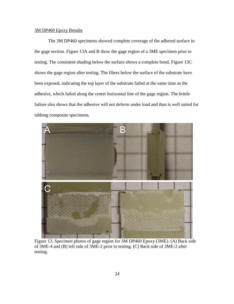
3M DP460 Epoxy Results
The 3M DP460 specimens showed complete coverage of the adhered surface in
the gage section. Figure 13A and B show the gage region of a 3ME specimen prior to
testing. The consistent shading below the surface shows a complete bond. Figure 13C
shows the gage region after testing. The fibers below the surface of the substrate have
been exposed, indicating the top layer of the substrate failed at the same time as the
adhesive, which failed along the center horizontal line of the gage region. The brittle
failure also shows that the adhesive will not deform under load and thus is well suited for
tabbing composite specimens.
Figure 13. Specimen photos of gage region for 3M DP460 Epoxy (3ME). (A) Back side
of 3ME-4 and (B) left side of 3ME-2 prior to testing. (C) Back side of 3ME-2 after
testing.
A B
C
25
The 3M DP460 epoxy had the highest failing force of the three tested adhesives.
In addition, the 3M DP460 epoxy also was the most workable due to its long set time and
relatively low viscosity after mixing. The only drawback is that the specimens require a
48 hour cure time.
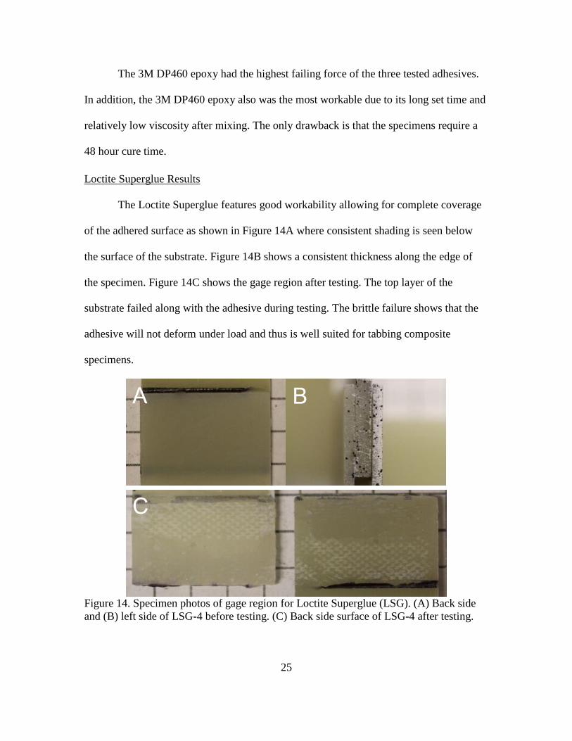
Loctite Superglue Results
The Loctite Superglue features good workability allowing for complete coverage
of the adhered surface as shown in Figure 14A where consistent shading is seen below
the surface of the substrate. Figure 14B shows a consistent thickness along the edge of
the specimen. Figure 14C shows the gage region after testing. The top layer of the
substrate failed along with the adhesive during testing. The brittle failure shows that the
adhesive will not deform under load and thus is well suited for tabbing composite
specimens.
Figure 14. Specimen photos of gage region for Loctite Superglue (LSG). (A) Back side
and (B) left side of LSG-4 before testing. (C) Back side surface of LSG-4 after testing.
A B
C

26
The Loctite Superglue has 80% the ultimate force of the 3M DP460 epoxy. While
the ultimate force is lower, the Loctite Superglue is an acceptable epoxy when test
specimens have to be ready for testing within a few hours.
J-B Weld KwikWeld Adhesive Results
During testing, complications with consistent adhesive application with the J-B
Weld adhesive led to having just 2 acceptable replicates. Figure 15A shows the back side
of a specimen in which the adhesive is evenly applied. However, the entire region was
not covered as seen in the gap in the top-right corner of the gage region. Figure 15B
shows a sample with the adhesive applied with a consistent thickness. The results after
testing show a variety of failure patterns in the adhesive. Figure 15C shows the adhesive
flaking away from the substrate indicating the bond with the surface was incomplete.
Figure 15D shows the adhesive experienced a brittle failure similar to those in the 3ME
and LSG specimens. Figure 15E shows a ductile failure in which the adhesive did not
completely fracture upon failure. The failure shown in Figure 15D is preferred, but the
inconsistent performance even within the same specimen illustrate the difficulty of using
the JB Kwik adhesive. The inconsistent failure patterns also correspond to the
inconsistent results shown in Table 7.
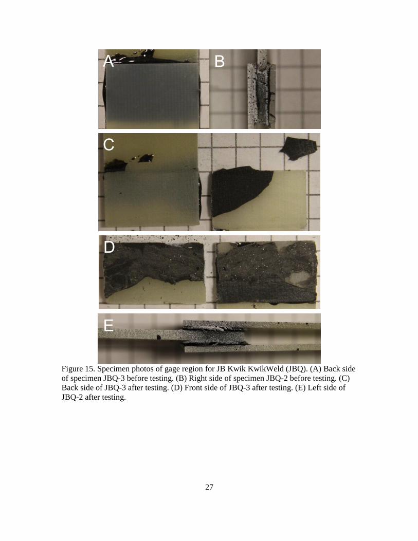
27
Figure 15. Specimen photos of gage region for JB Kwik KwikWeld (JBQ). (A) Back side
of specimen JBQ-3 before testing. (B) Right side of specimen JBQ-2 before testing. (C)
Back side of JBQ-3 after testing. (D) Front side of JBQ-3 after testing. (E) Left side of
JBQ-2 after testing.
A B
C
D
E

28
3 Experimental Data Processing Software Development
Determining the material properties from experimental data relies on processing.
With the goal of improving the ease of use for data processing for unidirectional
composites, the Experimental Data Processing (EDP) program is in ongoing
development. EDP features functionality to allow for complete processing. Greater detail
about this process is listed in 3.2. The general steps for post-processing are as follows.
Step 1. Read in the raw data. Raw data for composite testing is stored in two files
with strain and force measurements taken over time.
Step 2. Process the raw data. Raw force data must be normalized by converting it
to stresses. Raw data may also have inconsistent indexing, making unit
conversions potentially important.
Step 3. Smooth the processed data. Raw data may include noise that is inherently
a part of the testing process. Small irregularities during testing may also create
outliers in the data. Smoothing removes these irregularities from the data.
Step 4. Plot the stress and strain data together.
Step 5. Generate the model curve from the stress-strain curves of each replicate.
3.1 Overview
EDP is an existing program developed at ASU since 2010. The program has
evolved over time and is currently being developed for use with the MAT213 constitutive
model. New features have concentrated on implementing the full data processing process.
The most substantial improvement made to the program is the introduction of locally
weighted least squares smoothing methods for both data smoothing and outlier removal.
Smoothing functions already in place prior to improvement such as Moving Median and

29
Moving Average filters have also had bugs removed to improve accuracy and utility.
New features such as data inversion and data set creation were added to increase
efficiency. In addition to the processing improvements, an improved user interface has
been implemented to help with viewing relevant information on the data being modified.
The functions within EDP used in generating model curves from raw data are covered in
greater detail in Appendix C.
3.2 Processing Steps
Processing data in EDP for use in MAT213 involves a simple series of steps. A
full guide detailing all processing steps within EDP is found in chapter 4.
Prior to processing, the following information is required: raw DIC/MTS data,
cross-sectional area, the test type, and the capture rate. As detailed in chapter 4, raw data
for a single test is stored in two separate files: a CSV file with DIC data and a DAT file
with force data. The test type is important to determine where to measure the cross-
sectional area and the direction over which the strain is calculated. The capture rate for
the DIC cameras is important to translate the raw strain indices to time.
3.2.1 Step 1. Read Raw Data
The raw data can be read without any prior modifications, though it is also
important to note which columns store the relevant data (e.g. when reading raw DIC data,
only the index and exy columns are necessary for a shear test even if exx and eyy data are
also exported. The user should be aware of other analysis regions in addition to the
overall average if present). For a single test, multiple replicates are imported. To avoid
confusion, all replicates should be named appropriately and have the correct delimiter
selected. In total, six to ten files are read in depending on the number of replicates tested.

30
3.2.2 Step 2. Data Processing
Force and time data is used to determine the stress over time during the test. The
stress in a specimen is considered the force applied over the cross section over which the
load is applied. In a tension or compression specimen, the cross-section is in the direction
of loading and is determined from the average of measurements taken in the region of
failure prior to testing. Average stress in the specimen is calculated as follows.
A
F (2)
where F is the force applied at a single time point and A is the average cross-sectional
area. In shear, the cross-section is parallel to the applied load. For Iosipescu tests, this
area is between the notches. The average stress in the specimen is calculated as follows.
A
V (3)
where V is the shear force applied at a single time point and A is the cross-sectional area.
The strain data is calculated from the DIC images using Vic 3D 7® software. Depending
on the test, different stain types are needed. In shear tests, Vic 3D 7® calculates
engineering strain, requiring all strain values to be multiplied by two to convert to
tensorial strain.
For both strain and force data, the time columns must start at zero and have
consistent units. The strain indices must be converted to seconds based on the camera
capture rate.
3.2.3 Step 3. Smoothing
In most cases, there is a level of noise within the raw data. To remove this, EDP
has many different methods for smoothing data. The strengths and weaknesses for each

31
method are outlined in section 3.3.6. For characterization tests at ASU, simple moving
average (SMA) method is used.
3.2.4 Step 4. Plotting Stress-Strain Curves
After modifying the data, the stress and strain data must be reformatted so the
time steps match. To do this, EDP has a reformat command that will rediscretize the data
based on consistent time steps from a start time zero to a defined end time. Discretization
is performed by interpolating between existing smoothed data points to generate new
points. The end time is determined from matching time points in the force and strain data
corresponding to the point of failure. Both strain and stress data must have the same start
and end times and the same number of points.
Once all replicate data is reformatted over time, the stress data can now be plotted
against the strain data for each replicate.
3.2.5 Step 5. Generating the Model Curve
The model curve is the final result that is used as input for MAT213 and is
generated in four steps. First, the average ultimate strain is determined and is used as the
end point of the model curve. Second, each replicate curve is either cut or extended to
ensure all curves have the same end point determined from the average. If a replicate has
a smaller ultimate strain than the average, the final point is extrapolated from the final
points of the actual test. Similarly, if a replicate has a larger ultimate strain, the data is cut
so it ends at the average. Third, each curve is rediscretized so all strain points match.
From these points, the average stress is calculated and plotted to form the final model
curve.

32
3.3 Implementation
The current version of the program has the following capabilities: editing raw
data; Chauvenet’s criterion for removing outliers; moving median, simple moving
average (SMA), and polynomial moving average (PMA) filtering methods; curve
reformatting; and curve averaging. These capabilities were enhanced with the addition of
Lowess and Loess smoothing strategies and new implementation strategies for curve
averaging techniques.
3.3.1 Curve Averaging
One new function creates the best fit of all curves currently being active (plotted)
in the interface. The Generate Mean Curve function follows the post-processing steps
detailed in section 3.2.
Step 1. Based on active flags for plotting, the function counts the number of active
curves n and stores each corresponding replicate number j and data type (either
raw, smoothed, or fitted). Knowing the usable curves, the program pulls the
number of points Pj and the x and y column numbers for each active replicate.
Step 2. EDP next finds the average end strain based on the currently plotted data.
The function allows for the largest, smallest, or average end strain value to be
calculated and used.
Step 3. A new data set is created within the program that will contain the new x-
column, the new average y-column, and the rediscretized y-columns for each
input data set.
Step 4. Then, it discretizes the new x-axis (strain) array based on a starting point
of zero and the new end strain. Each original data set is then cut or extended as

33
needed based on the current end strain. To rediscretize the y values for each
replicate, the function loops through each replicate then loops through each point
within. When a rediscretized point xk lies between two points in an original curve
xi and xi-1, EDP interpolates between the original points to create the new stress
value yk.
1
1
ii
ii
xx
yym (4)
11 iikk yxxmy (5)
Once a curve is reformatted, the program loops through each of the k points and
begins to calculate the average as yk/n.
3.3.2 Lowess/Loess Theory
Loess (Local regression) and Lowess (Locally weighted scatterplot smoothing)
are similar methods for smoothing scattered data using a function based on weighted
parameters to perform multiple local weighted regressions. Lowess uses a linear
regression while Loess uses a higher degree polynomial for local fits (The MathWorks,
Inc. 2016).
Lowess smoothing utilizes a function of the following form.
0 1i iS x w w x (6)
0w and 1w are linear weight parameters generated within a local set of data defined by
the user. Loess uses a similar form function for polynomial fitting.
The weight function has four properties.
1. 0W x for 1x

34
2. W x W x for 1x
3. W x is a nonincreasing function for 0x
4. 0W x for 1x
While any weight function with those four properties will work, EDP uses the
normalized tri-cube weight function, which is of the following form.
33
1 ii i
x xw x
d x
(7)
where x is the focus point around which the local fitting function is formed, d x is the
distance between the focus point and the farthest point in the local array, and ix is the ith
point in the local array. This function is utilized i times (the number of user defined
points used to create the local fit) for all points n.
QR decomposition is used to calculate the least squares solution. Based on this
solution, the slope and intercept of the local line are determined and used to calculate a
new y-value based on each x-value. This process may be repeated for several iterations.
Note that when using the Loess algorithm, outliers have a more extreme effect on
the surrounding smoothed data in certain cases; Loess is only recommended for sets of
data with a large number of points and a high number of local points. Lowess is
satisfactory in all other cases.
3.3.3 Lowess Algorithm
Input: Set of data (x,y), number of points to be used for local regression (N), number of
repetitions (R), number of points within complete data set, P.
Output: Smoothed data
Step 1. Get the size of the data (s)

35
Step 2. Set ( 1) 2u N
Step 3. Loop through each point of focus i = 1 to i = P for R iterations
Step 3a. Establish local arrays of x and y data and determine the distance values, d, based
on location within the global array.
- If i u (focus is on left)
d x N x i (8)
- If i s u (focus is on right)
1d x i x P N (9)
- Else (focus is in the center range of data)
max 1 , 1d x i x i u x i u x i (10)
Step 3b. Calculate the weight of each point in the local array j based on the focus point i.
- ( ) ( )
j
x j x iz
d
(11)
- 3
31j jw z (12)
Step 3c. Begin QR decomposition. Set up the following matrices.
1
1
1
1
j
j
N
x
xx
x
(13) 1
j
j
N
y
yy
y
(14)
0.5
1
0 0
0 0
0
0 0 0
j
j
half
N
w
ww
w
(15)
- half halfx w x (16)
- Perform QR decomposition on halfx and calculate QÁ
- half halfy Q w y Á (17)
Step 3d. Calculate local slope and intercept from the following values of the halfy and R
matrices.
-
2,1
2,2
halfym
R (18)
- 1,2
1,1
1,1
halfy R mb
R
(19)
Step 3e. Calculate the new smoothed point based on equations (18) and (19).
- i new iy mx b (20)

36
Step 3f. Calculate the residuals (necessary for robust Lowess, see section 3.3.5).
For an example showing how to implement Lowess for a sample set of data, see
Appendix A.
3.3.4 Robust Local Regression Theory
Loess and Lowess methods for smoothing are both vulnerable to outliers. By
implementing a robust procedure, the Loess/Lowess methods can become resistant to a
small number of outliers. After following the Loess/Lowess procedure described in the
previous section for one iteration, the residual for each point can be calculated.
i i ir y y (21)
Where ri is the residual, iy is the smoothed value, and yi is the recorded value.
From these residuals, a robust weight value can be calculated for each ith point,
which is based on a bi-square function with the following constraints.
22
1 66
0 6
ii
ri i
i
rr MAD
w r MAD
r MAD
(22)
Where MAD is the median absolute deviation of the residuals.
medianMAD r (23)
The data is then smoothed again using the same tri-cube weights as before now
multiplied by the robust weights. The residual values are also used to determine if a value
should be used in the Loess/Lowess procedure. If the robust weight of a point is 0, then
that point is not considered in determining the smoothed position of any point, including
itself; instead, the closest neighboring values with non-zero robust weights are used.

37
The robust version of the process may be repeated for several iterations.
Note that when using the Robust Loess algorithm, outliers have a more extreme
effect on the surrounding smoothed data in certain cases. As with Loess, Robust Loess is
only recommended for sets of data with a large number of points and a high number of
local points. Robust Lowess is satisfactory in all cases.
3.3.5 Robust Lowess Algorithm
This algorithm is continued from step 3 (performed for one iteration) of section 3.3.3.
Step 4. Calculate the residual weight based of each point i.
22
1 66
0 6
ii
ri i
i
rr MAD
w r MAD
r MAD
(22)
Step 5. Loop through each point of focus i = 1 to i = P for R iterations
Step 5a. Establish local arrays of x and y data and determine the distance values, d, based
on location within the global array. If a point has a residual weight of zero, do
not include it in the local arrays for smoothing. The local coordinate vector only
points with a residual weight. The x array no longer includes those points for
calculating d and corresponding weights, but are still used as focus points.
- If i u (focus is on left)
d x N x i (8)
- If i s u (focus is on right)
1d x i x P N (9)
- Else (focus is in the center range of data)
max 1 , 1d x i x i u x i u x i (10)
Step 5b. Calculate the weight of each point in the local array, j, based on the focus point,
i. Note again that x values belonging to points with zero residual weight are
excluded from this step and the next closest neighbor is used instead. 3
3( ) ( )
1j ri
x j x iw w
d
(22)

38
Step 5c. Begin QR decomposition for least squares. Set up the matrices in equations
1
1
1
1
j
j
N
x
xx
x
(13) 1
j
j
N
y
yy
y
(14)
0.5
1
0 0
0 0
0
0 0 0
j
j
half
N
w
ww
w
(15),
and (16). Perform QR decomposition on halfx , calculate QÁ , and calculate
halfy (see
equation (17)).
Step 5d. Calculate local slope and intercept from the following values of the halfy and R
matrices using equations (18) and (19).
Step 5e. Calculate the new smoothed point using equation (20).
For an example showing how to implement Robust Lowess for a sample set of
data, see Appendix B.
3.3.6 Comparison of Smoothing Strategies
EDP features many smoothing methods. moving median, simple moving average
(SMA), polynomial moving average (PMA), Lowess, Loess, and the robust forms of
Lowess and Loess. Each smoothing method has benefits and drawbacks for different data
types. This section details scenarios for each smoothing type using actual data from
quasi-static load tests on unidirectional composite specimens.
In general, increasing the number of points or the number of iterations will
improve results. These variables should be selected based on the quality of the raw data.
Changing the variables multiple times may be required to achieve desired results.
Four sample data sets are discussed for each method. Case 1 involves longitudinal
strain data gathered from a 3-direction compression specimen using DIC shown in Figure
16. This data set features several minor plateaus that are common in raw compression test
data. In addition, the data is constantly increasing, meaning there are no outliers. The

39
original raw data has been modified to convert indices to units of time and to ensure the
data starts at zero. With only 54 points, processing this data shows the effects of each
method on a relatively small data set.
Figure 16. Raw strain data from 3-direction compression test (case 1).
Case 2 covers the stress data from the same 3-direction compression test, shown
in Figure 17. Like case 1, this case also features plateaus common with compression tests
with constantly increasing values. Unlike case 1, there are 266 points in this data set,
opening up new possibilities in processing options.

40
Figure 17. Raw stress data from 3-direction compression test (case 2).
Case 3 covers strain data from a 2-3 plane shear test featuring an anomalous
reading in the center of the data, shown in Figure 18. The data was identified as
anomalous based on a comparison with the raw force data for the same test, which did
not include a corresponding jump. While there is no real outlier in this data set, certain
smoothing options are preferred in this case. In processing, this data set will be cut at the
point of failure at around 1050 seconds.

41
Figure 18. Raw engineering strain data from 2-3 plane shear test (case 3).
The final case shows 1-3 plane shear test data that includes several plateaus and
possible outliers (see Figure 19). In processing, this data set will be cut at the point of
failure at around 130 seconds.

42
Figure 19. Raw stress data from 1-3 plane shear test (case 4).
3.3.6.1 Moving Median Filter
The Moving Median Filter is a simple filter that replaces each point with the
median value of the local points (Vokshi 2011). Mathematically, this is expressed as.
),...,,...,(][
uiiui
N
i yyymedm
(24)
where i is the current point ranging from 1 to P, P is the number of points within the data
set, 2
1
Nu , N is the local span size or number of points within the local range that the
filter processes for each point, and ][N
im is the new value of yi. This filter can only
process points from i=u+1 to i=P-u. The points at each end are unchanged.
Having relatively few points that are monotonically increasing will limit the
effectiveness of the median filter. In case 1, using the median filter results in no change in
the data (shown on the left in Figure 20) because any point value will always be in the
center of the local region. Similarly, Median will have no effect on the constantly
increasing data in case 2 (shown on the right in Figure 20).

43
Figure 20. Moving Median Filter. Case 1 (top) and Case 2 (bottom)

44
In case 3, the anomaly in the data results in a single plateau. Similar to Cases 1
and 2, Median filter has a limited effect on the data, as shown on the left in Figure 21.
The noise in this case, however, is somewhat mitigated by using the median filter, as
shown in the zoomed part of the plot on the bottom in Figure 21.

45
Figure 21. Case 3 smoothened with Moving Median Filter. Full plot (top) and zoomed
plot (bottom).

46
Case 4, with several outliers, allows for a more effective use of the Median filter.
When using more points, the median filter smooths outliers better than when using fewer
points. Figure 22 shows how the number of points effects smoothing. In this case, using a
wider range helps smooth regions with outliers. As with the previous cases, large jumps
without outliers are not smoothened by this method.

47
Figure 22. Case 4 smoothened with Moving Median Filter using 3 points (top) and 25
points (bottom).

48
3.3.6.2 Moving Average Filters
The two types of moving average filters are Simple Moving Average (SMA) and
Polynomial Moving Average (PMA). These are simple filters that replace each point with
the non-weighted average value of the local points (Vokshi 2011). Mathematically, this is
expressed as
[ ]
u
j
j uN
i
y
yN
(25)
where i is the current point ranging from 1 to P, P is the number of points within the data
set, 2
1
Nu , N is the local span size or number of points within the local range that the
filter processes for each point, j is the local index for the running average, and [ ]N
iy is the
new value of yi. This filter can process all points except the start and end point for SMA
and the first and final 2 points for PMA.
In case 1, with few points and no outliers, SMA and PMA are very effective at
smoothing these plateaus. In this case, using 9 points necessitates only 1 iteration, though
using 3 points requires 3 iterations to generate a comparable smoothed curve. Figure 23
shows the results of using SMA and PMA (third degree) both with 9 points and 1
iteration with similar results. Also note the ends of the smoothened data when using PMA
remain unchanged, limiting the effectiveness of PMA on data sets with few points.
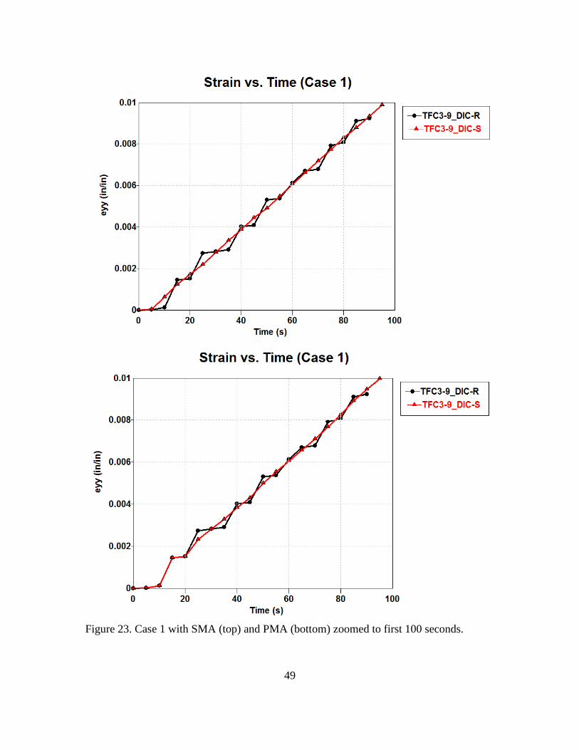
49
Figure 23. Case 1 with SMA (top) and PMA (bottom) zoomed to first 100 seconds.

50
With more points and large plateaus as in case 2, more local points are needed for
SMA and PMA to achieve adequate smoothing. In this case, 13 is the best number of
points needed for 1 iteration. Using fewer points with more iterations will be inadequate
in this case while using more will introduce new issues with overcorrecting. This case
also illustrates how PMA is susceptible to local patterns. With these plateaus, the curved
smoothed with PMA will closely match the original curve. More points and iterations are
needed to adequately smooth the data with PMA, though PMA’s issues with the ends of
the data set are apparent. Figure 24 shows the results of using SMA and PMA both with 9
points and 1 iteration. Note the local patterns adhered to by the PMA filter.

51
Figure 24. Case 2 smoothened with SMA (Top) and PMA (Bottom) zoomed to first 50
seconds.

52
Case 3 illustrates a case in which both a large number of iterations are necessary
and PMA is not adequate. Using SMA with 25 points and 15 iterations is necessary to
overcome the anomaly. Using PMA with an increasing number of iterations does not
approach a smooth line. Figure 25 compares the SMA results with PMA results using 25
points and 30 iterations.

53
Figure 25. Case 3 smoothed with SMA (top) and PMA (bottom) methods.

54
SMA works well with data involving few noticeable outliers. PMA, however,
shows susceptibility to local patterns, requiring more local points and more iterations.
Figure 26 shows the results of using SMA and PMA in case 4 with the same inputs.

55
Figure 26. Case 4 smoothened with SMA (left) and PMA (right) using 15 points and 2
iterations zoomed to initial 125 seconds.

56
3.3.6.3 Lowess/Loess
Loess (Local regression) and Lowess (Locally weighted scatterplot smoothing)
are similar methods for smoothing scattered data using a function based on weighted
parameters to perform multiple local weighted regressions. Lowess uses a linear
regression while Loess a higher degree polynomial for local fits. This filter allows for all
points within a given set to be processed. For more information on these methods, see
section 3.3.2.
This method is commonly used with high noise data, which is more common with
high strain-rate testing than with quasi-static testing. The cases detailed here use data
from quasi-static tests alone as high-strain rate test data for the same T800-F3900
composite is not currently available.
With case 1, Lowess and Loess methods offer similar functionality to SMA/PMA.
With 9 points and 1 iteration, Lowess/Loess appear very similar to the results shown in
Figure 23. While the two smoothed curves shown in Figure 26Figure 27 do not match,
the overall trends are acceptable for a final smoothed curve. Note that these methods
modify all points within the data set including the ends. Shifting the curve to ensure it
starts at the origin may be necessary. Shifting should only be done if the shift is small
relative to the maximum. In this case, the shift would be equal to about 1% of the
maximum value.
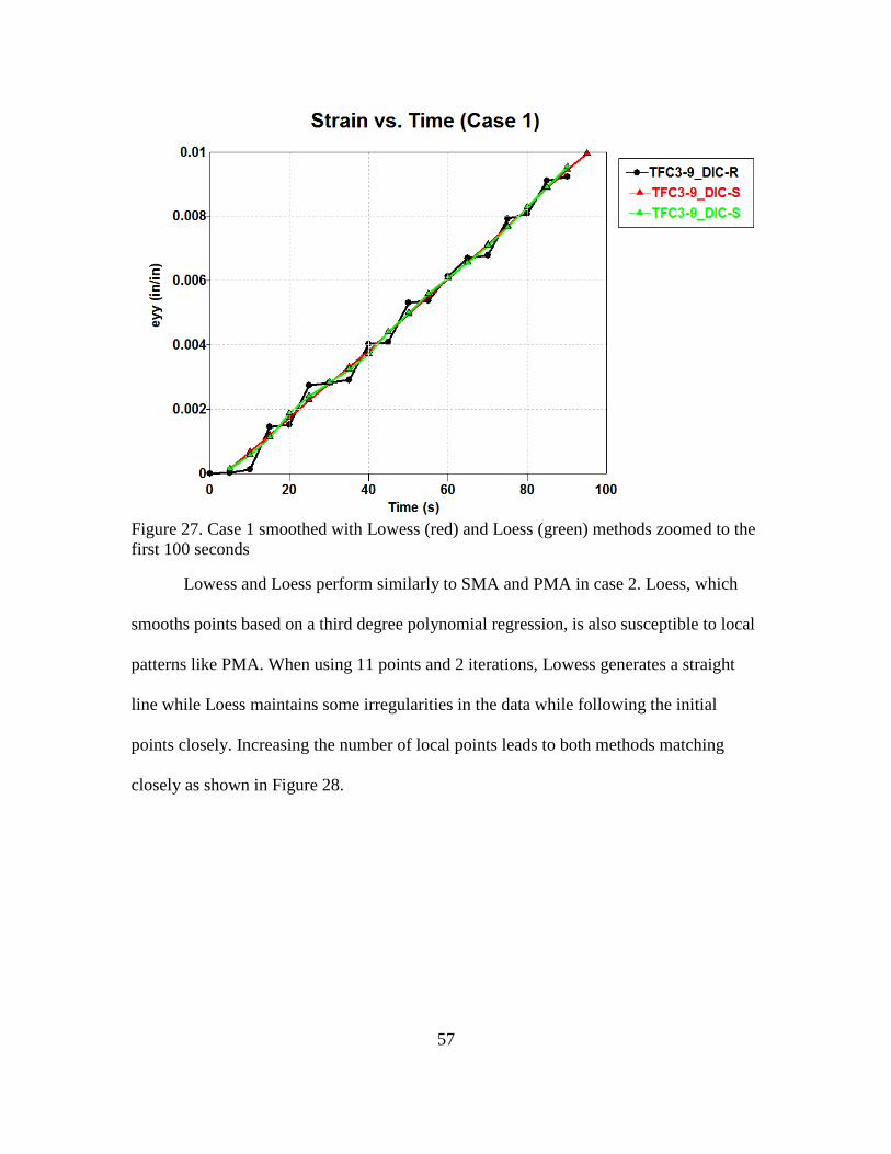
57
Figure 27. Case 1 smoothed with Lowess (red) and Loess (green) methods zoomed to the
first 100 seconds
Lowess and Loess perform similarly to SMA and PMA in case 2. Loess, which
smooths points based on a third degree polynomial regression, is also susceptible to local
patterns like PMA. When using 11 points and 2 iterations, Lowess generates a straight
line while Loess maintains some irregularities in the data while following the initial
points closely. Increasing the number of local points leads to both methods matching
closely as shown in Figure 28.

58
Figure 28. Case 2 smoothened with Lowess (red) and Loess (green) methods zoomed to
the first 50 seconds with 11 points (top) and 15 points (bottom)

59
Lowess and Loess do have some weaknesses compared to SMA and PMA. When
increasing the number of points and iterations as was done in Case 3 for SMA, the
computation time increases dramatically for Lowess and Loess. For case 3, using 25
points and 15 iterations is inadequate for both Lowess as shown in Figure 29. Just like
PMA, Loess smoothing does not converge on a smooth line in this case.
Figure 29. Case 3 smoothed with Lowess method.
In further contrast to SMA and PMA, Lowess and Loess are more susceptible to
outliers. Looking at some of the outliers in case 4, neither Lowess nor Loess methods are
able to smooth outliers as well as SMA. As shown in Figure 30, both methods result in
inadequately smoothened data around large outliers without increasing the number of
local points or iterations.

60
Figure 30. Case 4 smoothened with Lowess (red) and Loess (green) methods zoomed in
to show local outliers
Overall, Lowess and Loess methods follow local trends very closely. In data with
a high amount of noise, these local trends may be desirable. In materials testing, however,
local trends may not be indicative of the material response. The choice between Lowess
and Loess lies in the desired sensitivity to local phenomena in the data.
3.3.6.4 Robust Lowess/Loess
By implementing a robust procedure, the Loess/Lowess methods can become
resistant to a small number of outliers. The robust procedure involves using
Lowess/Loess method for one iteration, then determining the residual for each point
based on that iteration. This residual is used as an additional weight to reduce the impact
of relative outliers. This filter allows for all points within a set to be processed. For more
information on these methods, see section 3.3.4.

61
Including the residual weights only helps with outliers, however. In cases 1, 2,
and 3, without any outliers, Robust Lowess/Loess does not appear any different from
their non-robust results. The results in case 3 are shown in Figure 31.
Figure 31. Case 3 smoothened with Robust Lowess (red) and Robust Loess (green)
methods.
In case 4, the robust version of Lowess and Loess smoothen large outliers better
than their basic counter parts as shown in Figure 32.

62
Figure 32. Case 4 smoothened with Robust Lowess (red) compared to Lowess (green).
4 Post-Processing to Generate Input for Constitutive Model
This chapter illustrates the complete process for processing raw data from
multiple tests to generate a representative curve for the tension response of the 2-
Direction of the T800S/3900-2B unidirectional composite. All model curves generated in
EDP based on the ASU tests for the T800S/3900-2B composite are found in Appendix C.
Upon launching the program, note the basic commands available. The tool bar at
the top includes several buttons. At the far left is the New button, which will clear all
current data and present the screen as it is at startup. Next is the Open button, with which
you may open a previously saved .edp file. The Save button is to the right of open and
saves all work as currently stored. To get started, select Read raw data located in the
toolbar as highlighted in red in Figure 33.

63
Figure 33. Step 1 of processing involves reading in the raw data. The Read raw data button
(highlighted in red) is found at the top of the screen in the tool bar.
Once pressed, you will be presented with the Read Raw Data interface detailed in
Figure 34. The first step is to Browse folders for one data file to be processed. Be sure to
properly name each file prior to loading files.

64
Figure 34. The Read Raw Data interface. In here, multiple sets of data may be read in at
once before closing the interface.
After selecting the data file, a preview of the contents is shown at the bottom of
the window. Using this, it is a simple matter to fill in the Data ID (the name of the data
set or replicate), the number of columns, which columns are to be plotted as x and y-axes
(this can be changed later), and the number of header lines. Note the tip on the right that
specifies how to interpret the number of header lines.

65
It is important to differentiate between DIC and MTS data. In Figure 35, the DIC
data for replicate 3 has been labelled “TFT2-3_DIC” to indicate the test, the replicate
number, and the data being stored. In addition, since the DIC data is stored in a .csv file,
only the comma delimiter should be selected in the upper left corner. The number of
columns is determined for DIC by counting the number of commas in row one. Since
there are 3 commas, there are 4 rows. It may also be necessary to count columns outside
of EDP prior to reading raw data. For a tension test, the longitudinal strain is needed,
which labelled as eyy in column 3. Vic 3D 7® exports data with 2 header rows with the
analysis region in row 1 and the column title in row 2. Press apply to receive
confirmation that the replicate successfully read.

66
Figure 35. The Read Raw Data interface with DIC information entered.
Next, the MTS data is read. The MTS system exports force data using 5 header
lines, but one is blank. As noted in the tip, 4 is entered as the number of header lines to
accommodate. The MTS data is separated by tabs. The MTS data always has three
columns: Time, Actuator Displacement, and Force. Time and force are the columns of
interest. The Read Raw Data dialogue should appear as it does in Figure 36. Press Okay
when finished reading all data sets.

67
Figure 36. Read Raw Data dialogue with MTS data entered.
If a mistake is made when reading raw data, such as entering an incorrect number
of header lines, the command deleterep is available for use in the Edit Raw Data
dialogue box in the Action input box within the Cell Operations area (seen in Table 8).
Take care when deleting data sets as it is not possible to rearrange data sets at this time.
The raw data is immediately plotted upon pressing okay. DIC and MTS data are
on different scales, however, making visualization difficult at this point. Using the check
boxes on the top left of the viewing area, it is possible to toggle each curve on and off

68
(see Figure 37). When data is smoothened or fitted, toggling each smoothened or fitted
set of data will also be possible. The raw DIC and MTS data can now be visualized as
illustrated in Figure 38. Visualizing each data set helps to identify which smoothing
methods would work best. In the 2-Direction Tension test, data is consistent with some
noise. The drops at the end of each data set should be excluded from processing.
Figure 37. Plot toggle area in top left of view screen.

69
Figure 38. Raw data plotted in EDP.

70
To ensure all data set pairs match and are normalized, the raw data needs to be
edited. Select EDIT or view data at the top of the screen next to the Read Raw Data
button to view the data (see Figure 39).
Figure 39. Location of Edit or view data button
Upon opening the Edit Raw Data & View Smoothened and Fitted Data, data from
data set one is presented by default. Note the four major areas within this interface shown
in Figure 40. At the top is list data showing relevant data for all replicates, including the
set number, set name, the number of points, the number of columns, etc. The main feature
is the data visualization in the center of the interface. Row ID’s are shown on the left
while column headers and units are shown above the column ID’s. The currently selected
data is viewable and editable in this area. Here, it is possible to insert rows/columns,
delete rows/columns, and cut, copy, paste, and clear data using right click. To delete or
insert, the header must be selected. On the bottom right of the window are the details of

71
the data set currently on screen. Here, set name, column headers, column units, and the x
and y-columns can be changed. This is also where the current data set and data type are
selected for the viewing area. For a data change made in the details or viewing areas to be
stored, the Update button must be pressed. Export will create a new text file with the x
and y data separated by commas. Finally, in the upper right is the Cell Operations area.
Here, Actions can be entered to modify raw and smoothened data. Current commands are
shown in Table 8.
Figure 40. Edit Raw Data & View Smoothened and Fitted Data interface upon launch.
Table 8. Functions for editing data.
Function Description Format
Edit Raw Data Edits an existing column or
creates a new column
within a data set based on
an equation. Uses column
ID available at the top of
the viewing window.
ds?_c?_raw = expression involving
other columns

72
Delete Replicate Deletes a data set. deleterep, replicate #
Reformat Rediscretizes smoothened
data within a zone of a data
set based on an existing
column.
reformat, replicate #, zone #, x
column #, # of points
Create Creates a new data set from
existing data sets.
create, replicate name, type, x
replicate #, x column #, y replicate
#, y column #
Zero Shifts a column to start at
zero.
zero, replicate #, column #
Invert Inverts a column. inv, replicate #, column #
Zero and Invert Performs both the Zero and
Invert functions
zeroinv, replicate #, column #
The first step of editing data is normalizing values. The zero and invert commands
are used here to ensure all sets of data start at zero time, zero strain, and zero stress as
long as the initial values are small compared to the maximum values. For example, MTS
time starts at 1.05322 seconds, despite representing the start of the test. Another example
is the force column. For TFT2-3, the max force is 394.802 while the initial force is
1.47709, or about 0.4% of the maximum value. The zero command allows for multiple
replicate and column pairs to be entered at once (e.g. zero, 1, 1, 1, 3, 5, 1, 5, 3 indicates
the first and third columns of data sets 1 and 5 are to be zeroed). Since this is a tension
test, there is no need to invert the data. Compression and shear tests may require inverting
the data.
Once data is zeroed, the raw data must now be normalized. The DIC data is
presented by index instead of time. The capture rate should be recorded during testing.
For TFT2 tests, the capture rate was 3. By using the command
“ds1_c1_raw=ds1_c1_raw*3”, the indices are converted to units of time. MTS data also
shows force instead of the normalized stress. Using the edit raw data function, the force

73
can be converted to stress. To reflect these conversions, use the Details of Data Set area
to update the column titles and units.
The changes made should be immediately apparent upon pressing Okay in the
Edit Raw Data dialogue box.
Next, the data must be smoothed. Now that data is loaded, the Process Data
button is available. Select the Process Data button in the top tool bar as shown in Figure
41.
Figure 41. Interface with Process data button highlighted
The Data Set-Zone Data dialogue box is where smoothing and fitting options are
selected, shown in Figure 42. Here, all changes to the current Data Set will only be stored
upon pressing Update.
Smoothing and fitting is done by zone. If a data set has multiple regions of data
(ex. linear and nonlinear regions), additional zones may be added with the Add Zone
button on the right. Zones are defined by the start and x values. These values should
correspond to those from the x-column defined upon reading or editing data. For the 2-

74
Direction tension tests, the start x should be 0 and the end x depends on the ultimate
stress and strain values for each replicate. All end values should be multiples of 3 to
ensure stress and strain points match. The current fit types and smoothing methods are
outlined in Table 9 and Table 10. The number of points must be odd between 3 and 25
for most smoothing methods; PMA and Loess require a minimum of 5 points.
Figure 42. Data Set-Zone Data dialogue box
Since the data appears straight with a small amount of noise, an appropriate
smoothing method must be selected. For this example, both SMA and Lowess smoothing
are used. Additional information on smoothing methods is available in section 3.3.6. The

75
results of both methods are shown in this guide. Select analyze once all zones are defined
and press OK once the analysis is finished.
Table 9. Fitting Types and their descriptions
Fitting Type Description
Polynomial Fits the data within the zone to a first, second, third, fourth, or
fifth degree polynomial.
Exponential Fits the zone data to an exponential curve of the form bxy ae
Logarithmic Fits the zone data to a logarithmic curve of the form
logy a bx
Power Fits the zone data to curve of the form by ax
Table 10. Smoothing Methods and brief descriptions.
Smoothing Type Description
Median Replaces data points with the median value of a local range.
Simple Moving
Average
Replaces data points with the unweighted average value of a
local range.
Polynomial Moving
Average
Replaces data points with the weighted average value of a
local range.
Loess Replaces data points with a weighted value calculated using
local regression (using a second degree polynomial) within a
local range giving more weight to proximate values.
Robust Loess Loess with an additional weight considering outliers.
Lowess Replaces data points with a weighted value calculated using
local regression (using a first degree polynomial) within a
local range giving more weight to proximate values.
Robust Lowess Lowess with an additional weight considering outliers.
Once analyzed, the Smoothened Data is now able to be toggled on the left. Figure
43 shows the TFT2 smoothened data generated using Lowess with 15 points and 2
repeats.

76
Figure 43. Smoothened data generated with Lowess smoothing plotted in EDP

77
Figure 44. Smoothened data generated with SMA method plotted in EDP
The smoothened data must now be reformatted with the “Reformat” command
(detailed in Table 8; ex. “reformat, 1, 1, 1, 200” rediscretizes data set 1, zone 1, based on

78
column 1 into 200 points) using the Action prompt within the Edit Raw Data & View
Smoothened and Fitted Data dialogue box.
Once all replicates are reformatted, the “create” command can be used (ex.
“create, TFT2-3, smt, 1, 3, 5, 3” will create a new replicate titled TFT2-3 based on the
smoothed data stored in column 3 of data set 1 and column 3 of data set 2). EDP alerts
the user when the new data set is successfully created. The column titles and units are
transferred from the source columns automatically. The results for creating the 4 stress-
strain curves for the 2-Direction tension test are shown in Figure 45.
Figure 45. Stress-strain curves for the four replicates plotted in EDP
With all stress-strain curves generated, the final step is to generate the best fit or
model curve. The Best fit plot button is in the top toolbar as shown in Figure 46.

79
Figure 46. Interface with Best fit plot button highlighted.
The Best Fit plot will be generated based on all curves currently being plotted.
When using Lowess or Loess smoothing, be sure all replicates start at 0 prior to creating
the best fit (other methods will maintain the same start and end points). Upon pressing
Best fit plot, the Best Fit Input dialogue box is presented, shown in Figure 47. There are
three inputs for creating the best fit: the new data set name, the curve end type, and the
number of data points. There are three curve end types: extend, average, and cut. Extend
selects the largest end x value as the end point for the best fit and extrapolates shorter
curves. Average takes the average of the end points and cuts/extends curves as needed.
Cut selects the smallest end x value as the end point for the best fit curve and cuts longer
curves. The number of points must be between 5 and 100. For this example, the name
will be set to “TFT2”, the end type set to “Average”, and the number of points set to 100.

80
Figure 47. Best Fit Input dialogue box
The final curve can then be plotted alone. For better visualization, change the plot
limits by pressing the Edit graph settings button in the top bar, as shown in Figure 48.
Figure 48. Interface with Edit graph settings button highlighted
The XY Graph Data dialogue box has two tabs. The first tab, Graph Attributes,
allows for the axis labels and graph title to be edited. The curve colors, markers, and line
types are also customized in this section. The Graph Layout tab allows for the plot limits

81
to be modified. In this tab are miscellaneous options to further customize the plot
appearance. Both tabs are shown in Figure 49.
Figure 49. XY Graph Data interface with the Graph Attributes tab (left) and Graph
Layout tab (right) shown
The final curve generated with Lowess and SMA smoothing methods with
modified plot limits and alternate y-axis are shown in Figure 50. Both curves are very
close together with the Lowess curve having a higher ultimate strain and the SMA curve
having a higher ultimate stress. Both curves appropriately represent the response of the
T800-F3900 composite in the 2-direction. When generating other curves, however, the
best smoothing method depends on the quality of the raw data.

82
Figure 50. Final model curve for TFT2 generated with Lowess (blue) and SMA (grey)
smoothing methods plotted in EDP

83
5 Conclusions
Composite materials are increasingly used in structural applications due to their
high strength-to-weight ratio and durability. FE material models are actively being
developed for modeling composites under load. FE models rely on characterization
testing for input values including Young’s modulus, Poisson’s ratio, stress-strain curves,
etc. Testing for unidirectional composites involves scenarios not seen in more commonly
tested materials such as metals. Tabbing strategies have been developed though rely
heavily on the characteristics of the adhesive used. Through the testing of three candidate
adhesives, a comparison has made to determine the best of the candidate adhesives for
use in the testing of composite materials. In addition, determining material characteristics
depends on post-processing strategies. The development of the EDP software has allowed
for a complete experience for generating some of the required inputs for the MAT213
constitutive model.
The results of the adhesives testing show that the 3M DP460 is the best
performing adhesive of the candidate adhesives based on double-lap shear tests for
tabbing unidirectional composites. The 3M epoxy achieved a shear strength of 3423.4 psi
on the G10 fiberglass substrate, which is 1 ksi below the reported shear strength on an
aluminum substrate. The Loctite Superglue has some useful functionality with 80% the
strength of the 3M DP460 epoxy and a much quicker cure time. The JB KwikWeld
proved inadequate for use with tabbing due to low workability and low apparent shear
strength.
In the realm of processing, EDP has received a large number of features and
improvements aimed at facilitating the post-processing of data for use with the MAT213

84
constitutive model. New locally weighted regression techniques have been implemented
to both improve upon the smoothing capabilities of the software and help remove outliers
from raw data. Additional supplementary functions have been implemented to allow for
improved ease of use while processing. Using the new processes implemented in EDP, 11
of the characteristic curves for the T800 composite have been generated for eventual use
in MAT213.
5.1 Future Work
The EDP currently lacks some supplementary functions for current functionality.
A foundation for the student’s t-test had been introduced previously but not fully
implemented. The ability to manipulate raw data is currently limited without the
introduction of potentially useful functions such as backward extrapolation. The program
will require the ability to easily determine the slope of a line as well as the area under a
generated curve.
The program also lacks major functionality for the post-processing of data for use
in MAT213. A function to generate flow rule coefficients and create the material card
based on data read into EDP would mean only one program is necessary for the
processing of raw data for use in MAT 213.

85
REFERENCES
3M. 2015. "Scotch-Weld DP460 Off-White Technical Data Sheet." St. Paul, MN, May.
Accurate Plastics, Inc. 2016. "Sheet Comparative Data Chart." Acculam. Accessed July
28, 2016. http://www.acculam.com/data-chart.html.
Adams, Daniel O., and Donald F. Adams. 2002. Tabbing Guide for Composite Test
Specimens. Washington, D.C.: U.S. Department of Transportation.
ASTM D 1002-10 Committee. 2010. Standard Test Method for Apparent Shear Strength
of Single-Lap-Joint Adhesively Bonded Metal Specimens by Tension Loading
(Metal-to-Metal). West Conshohocken, PA: ASTM International.
ASTM D 3528-96 Committee. 2008. Standard Test Method for Strength Properties of
Double Lap Shear Adhesive Joints by Tension Loading. West Conshohocken,
PA.: ASTM International.
Cleveland, William S. 1979. "Robust Locally Weighted Regression and Smoothing
Scatterplots." Journal of the American Statistical Association 829-836.
Correlated Solutions. 2014. "Vic-3D v7 Reference Manual." January 10.
Goldberg, Robert K., Kelly S. Carney, Paul DuBois, Canio Hoffarth, Subramaniam
Rajan, and Gunther Blankenhorn. 2015. Incorporation of Plasticity and Damage
Into an Orthotropic Three-Dimensional Model with Tabulated Input Suitable for
Use in Composite Impact Problems. National Aronautics and Space
Administration, Glenn Research Center.
Harrington, Joseph, Canio Hoffarth, Subramaniam D. Rajan, Robert K. Goldberg, Kelly
S. Carney, Paul Dubois, and Gunther Blankenhorn. 2016. "Using Virtual Tests to
Complete the Description of a Three-Dimensional Orthotropic Material."
submitted ASCE J of Aerospace Engineering.
Henkel. 2014. "Loctite Super Glue Longneck Bottle Technical Data Sheet." Dusseldorf,
March 5.
J-B Weld It Australia. 2012. "JB Kwik - Technical Data and Instruction Sheet." J-B Weld
It. January 08. Accessed July 12, 2016.
http://jbweldit.com.au/index.php?main_page=document_general_info&cPath=4&
products_id=10.
J-B Weld. 2014. "J-B Weld Safety Data Sheet." Sulphur Springs, TX, Nov 11.
Lin, Lily, and Paul D Sherman. 2007. "Cleaning Data the Chavenet Way." The
Proceedings of the SouthEast SAS Users Group. SESUG Proceedings. Paper
SA11.

86
Livermore Software Technology Corporation (LSTC). 2015. "LS-DYNA(R) Keyword
User's Manual Volume 1." March 23.
Matthews, F. L., P. F. Kilty, and E. W. Godwin. 1982. "A review of the strength of joints
in fibre-reinforced plastics. Part 2. Adhesively bonded joints." Composites 29-37.
Renton, W. James. 1976. "The Symmetric Lap-shear Test - What Good Is It?"
Experimental Mechanics 409-415.
Savitzky, Abraham, and Marcel J. E. Golay. 1964. "Smoothing and Differentiation of
Data by Simplified Least Squares Procedures." Analytical Chemistry 1627-1639.
Stroud, Phillip D. 1999. A Recursive Exponential Filter for Time-Sensitive Data. Los
Alamos: Los Alamos National Laboratory.
The MathWorks, Inc. 2016. Filtering and Smoothing Data. Accessed July 17, 2016.
www.mathworks.com/help/curvefit/smoothing-data.html.
Toray Carbon Fibers America, Inc. n.d. T800S Data Sheet. Technical Data Sheet, Santa
Ana: Toray USA.
Vokshi, Erblina. 2011. Experimental Investigation and Development of Finite Element
Model for Knife and Spike Impact. Masters Thesis, ASU: School of Sustainability
and the Built Environment.
Yang, Charles, John S. Tomblin, and Zhidong Guan. 2003. Analytical Modeling of ASTM
Lap Shear Adhesive Specimens. Washington, D.C.: U.S. Department of
Transportation, Federal Aviation Administration.

87
APPENDIX A
LOWESS EXAMPLE

88
Consider the set of data shown in Table 11.
Table 11. Lowess Example Data
x y
0 5
5 9
10 6
15 25
20 300
25 15
30 27
Step 1. The size of the data set is s = 7.
Step 2. Applying a span of five (N = 5, u = 3).
[5]
-x if
max 1 , 1 if 1
1 if 1
i
x N i i u
d x i x i u x i u x i u i P u
x i x P N i P u
3
3 5
5
i
i
i
Step 3. For i = 1 (x = 0)
Step 3a. [5]
1 5 1 20 0 20d x x
Step 3b. ' 0 5 10 15 20localx
1
1
(1) (1)0
localx xz
d
, 2
1
(2) (1)0.25
localx xz
d
,
3 0.5z ,4 0.75z ,
5 1z
3
3
1 11 1w z , 3
3
2 21 0.954w z ,3 0.670w ,
4 0.193w ,5 0w
Step 3c. Begin QR decomposition.
1 0
1 5
1 10
1 15
1 20
x
,
5
9
6
25
300
y
,
0.51 0 0 0 0
0.954 0 0 0
0.670 0 0
0.193 0
0
halfw
sym
1 0
0.977 4.883
0.819 8.185
0.440 6.594
0 0
half halfx w x
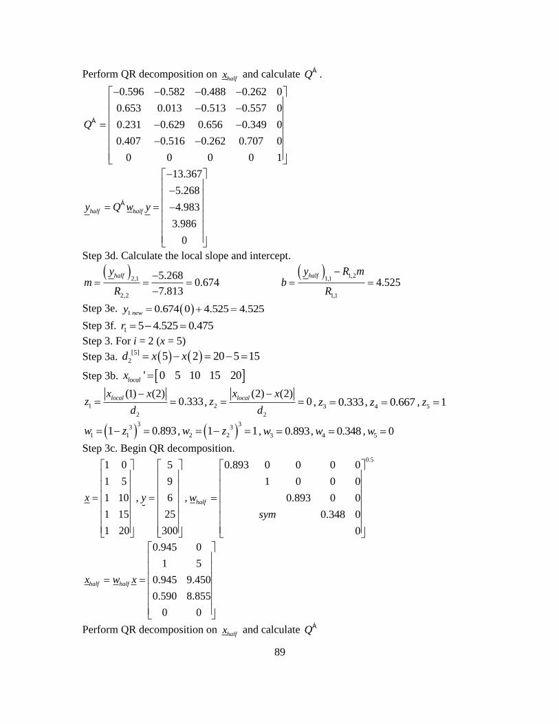
89
Perform QR decomposition on halfx and calculate QÁ .
0.596 0.582 0.488 0.262 0
0.653 0.013 0.513 0.557 0
0.231 0.629 0.656 0.349 0
0.407 0.516 0.262 0.707 0
0 0 0 0 1
Q
Á
13.367
5.268
4.983
3.986
0
half halfy Q w y
Á
Step 3d. Calculate the local slope and intercept.
2,1
2,2
5.2680.674
7.813
halfym
R
1,21,1
1,1
4.525halfy R m
bR
Step 3e. 1 0.674 0 4.525 4.525newy
Step 3f. 1 5 4.525 0.475r
Step 3. For i = 2 (x = 5)
Step 3a. [5]
2 5 2 20 5 15d x x
Step 3b. ' 0 5 10 15 20localx
1
2
(1) (2)0.333
localx xz
d
, 2
2
(2) (2)0
localx xz
d
,
3 0.333z ,4 0.667z ,
5 1z
3
3
1 11 0.893w z , 3
3
2 21 1w z ,3 0.893w ,
4 0.348w ,5 0w
Step 3c. Begin QR decomposition.
1 0
1 5
1 10
1 15
1 20
x
,
5
9
6
25
300
y
,
0.50.893 0 0 0 0
1 0 0 0
0.893 0 0
0.348 0
0
halfw
sym
0.945 0
1 5
0.945 9.450
0.590 8.855
0 0
half halfx w x
Perform QR decomposition on halfx and calculate QÁ

90
15.552
7.011
6.388
4.629
0
half halfy Q w y
Á
Step 3d. Calculate the local slope and intercept.
2,1
2,2
7.0110.8063
8.696
halfym
R
1,21,1
1,1
3.857halfy R m
bR
Step 3e. 2 0.806 5 3.857 7.888newy
Step 3f. 2 9 7.888 1.112r
Step 3. For i = 3 (x = 10)
Step 3a. [3]
3 max 5 3 , 3 1 max 20 10,10 0 10d x x x x
Step 3b. ' 0 5 10 15 20localx
1
3
(1) (3)1
localx xz
d
, 2
1
(2) (3)0.5
localx xz
d
,
3 0z ,4 0.5z ,
5 1z
3
3
1 11 0w z , 3
3
2 21 0.670w z ,3 1w ,
4 0.670w ,5 0w
Step 3c. Begin QR decomposition.
1 0
1 5
1 10
1 15
1 20
x
,
5
9
6
25
300
y
,
0.50 0 0 0 0
0.670 0 0 0
1 0 0
0.670 0
0
halfw
sym
0 0
0.819 4.092
1 10
0.819 12.277
0 0
half halfx w x
Perform QR decomposition on halfx and calculate QÁ and R
18.813
9.260
6.299
5.442
0
half halfy Q w y
Á
Step 3d. Calculate the local slope and intercept.

91
2,1
2,2
9.2601.600
5.788
halfym
R
1,21,1
1,1
3.701halfy R m
bR
Step 3e. 3 1.600 10 3.701 12.299newy
Step 3f. 3 6 12.299 6.299r
Step 3. For i = 7 (x = 30)
Step 3a. [5]
7 7 7 5 1 30 10 20d x x
Step 3b. ' 10 15 20 25 30localx
1
7
(1) (7)1
localx xz
d
, 2
7
(2) (7)0.75
x xz
d
,
3 0.5z ,4 0.25z ,
5 0z
3
3
1 11 0w z , 3
3
2 21 0.193w z ,3 0.670w ,
4 0.954w ,5 1w
Step 3c. Begin QR decomposition.
1 10
1 15
1 20
1 25
1 30
x
,
6
25
300
15
27
y
,
0.50 0 0 0 0
0.193 0 0 0
0.670 0 0
0.954 0
1
halfw
sym
0 0
0.440 6.594
0.819 16.370
0.977 24.416
1 30
half halfx w x
Perform QR decomposition on halfx and calculate QÁ and R
147.233
114.357
145.135
70.328
24.338
half halfy Q w y
Á
Step 3d. Calculate the local slope and intercept.
2,1
2,2
114.35714.637
7.813
halfym
R
1,21,1
1,1
452.177halfy R m
bR
Step 3e. 7 14.637 30 452.177 13.074newy
Step 3f. 7 27 13.074 13.926r
The smoothed data with each residual is shown in Table 12.

92
Table 12. Smoothed Lowess example data and residual data.
x y r
0 4.525 0.475
5 7.888 1.112
10 12.299 -6.299
15 98.296 -73.295
20 139.666 160.334
25 86.6836 -71.684
30 13.074 13.926
Figure 51. Lowess example data and smoothed data plots.
When visualizing the data in Table 12 as shown in Figure 53, it should be noted
that the outlier corresponding to y=300 has been reduced but not been eliminated, and the
surrounding data points have been skewed towards the outlier. Also note that following
the Loess algorithm, this outlier would have a more extreme effect on the surrounding
data, as shown in Figure 52. Therefore, Loess is only recommended for sets of data with
more points and a higher number of local points.

93
Figure 52. Example data with smoothed data generated with Loess method.

94
APPENDIX B
ROBUST LOWESS EXAMPLE

95
Consider the set of data shown in Table 13.
Table 13. Robust Lowess example data. The original data and corresponding residuals
from a single iteration of Lowess smoothing are shown.
x y r
0 5 0.475
5 9 1.112
10 6 -6.299
15 25 -73.295
20 300 160.334
25 15 -71.684
30 27 13.926
These steps continue from the process detailed in Appendix A.
Step 4. Determining MAD = 13.9256
Calculate weights based on residuals.
22
1 83.553683.5536
0 83.5536
ii
ri i
i
rr
w r
r
0.9999 0.9996 0.9887 0.0531 0 0.0697 0.9452riw
Step 5. For i = 1 (x = 0)
Step 5a. Apply a span of three (N = 5, u = 3).
Because point 5 is within the local range and wr5 = 0, this point must be ignored when
calculating weights for this section. Point 6 is used instead.
[5]
1 6 1 25 0 25d x x
Step 5b. ' 0 5 10 15 25localx
1
1
(1) (1)0
localx xz
d
, 2
1
(2) (1)0.2
localx xz
d
,
3 0.4z ,4 0.6z ,
5 1z
3
3
1 1 11 0.9999rw z w , 3
3
2 2 21 0.9758rw z w ,3 0.8107w ,
4 0.0256w ,5 0w
Step 5c. Begin QR decomposition.
1 0
1 5
1 10
1 15
1 20
x
,
5
9
6
25
15
y
,
0.50.9999 0 0 0 0
0.9758 0 0 0
0.8107 0 0
0.0256 0
0
halfw
sym

96
1 0
0.988 4.939
0.900 9.004
0.160 2.400
0 0
half halfx w x
Perform QR decomposition on halfx and calculate QÁ .
0.596 0.589 0.537 0.095 0
0.689 0.035 0.684 0.237 0
0.371 0.779 0.474 0.176 0
0.1807 0.212 0.137 0.951 0
0 0 0 0 1
Q
Á
11.501
1.515
3.214
2.081
0
half halfy Q w y
Á
Step 5d. Calculate the slope and intercept for local regression.
2,1
2,2
1.5150.219
6.903
halfym
R
1,21,1
1,1
5.815halfy R m
bR
Step 5e. 1 0.219 0 5.815 5.815newy
Step 5. For i = 2 (x = 5)
Step 5a. [5]
2 5 2 20 5 15d x x
Step 5b. ' 0 5 10 15 25localx
1
2
(1) (2)0.25
localx xz
d
, 2
2
(2) (2)0
localx xz
d
,
3 0.25z ,4 0.5z ,
5 1z
3
3
1 1 11 0.9538rw z w , 3
3
2 2 21 0.9996rw z w ,3 0.9430w ,
4 0.0356w ,5 0w
Step 5c. Begin QR decomposition.
1 0
1 5
1 10
1 15
1 25
x
,
5
9
6
25
15
y
,
0.50.9538 0 0 0 0
0.9996 0 0 0
0.9430 0 0
0.0356 0
0
halfw
sym
0.977 0
0.9998 4.999
0.971 9.711
0.189 2.830
0 0
half halfx w x
Perform QR decomposition on halfx and calculate QÁ

97
11.863
1.576
3.428
2.457
0
half halfy Q w y
Á
Step 5d. Calculate the slope and intercept for local regression.
2,1
2,2
1.5760.221
7.138
halfym
R
1,21,1
1,1
5.801halfy R m
bR
Step 5e. 2 0.221 5 5.801 6.905newy
Step 5. For i = 3 (x = 10)
Step 5a. [5]
3 max 6 3 , 3 1 max 25 10,10 0 15d x x x x
Step 5b. ' 0 5 10 15 25localx
1
3
(1) (3)0.667
localx xz
d
, 2
1
(2) (3)0.333
localx xz
d
,
3 0z ,4 0.333z ,
5 1z
3
3
1 1 11 0.349rw z w , 3
3
2 2 21 0.893rw z w ,3 0.989w ,
4 0.047w ,5 0w
Step 5c. Begin QR decomposition.
1 0
1 5
1 10
1 15
1 25
x
,
5
9
6
25
15
y
,
0.50.349 0 0 0 0
0.893 0 0 0
0.989 0 0
0.047 0
0
halfw
sym
0.590 0
0.945 4.724
0.994 9.943
0.218 3.267
0 0
half halfx w x
Perform QR decomposition on halfx and calculate QÁ and R
11.195
0.976
3.481
2.802
0
half halfy Q w y
Á
Step 5d. Calculate the slope and intercept for local regression.

98
2,1
2,2
0.9760.172
5.678
halfym
R
1,21,1
1,1
6.282halfy R m
bR
Step 5e. 3 0.172 10 6.282 8.001newy
Step 5. For i = 7 (x = 30)
Step 5a. [5]
7 7 2 30 5 25d x x
' 5 10 15 25 30localx
1
7
(1) (7)1
localx xz
d
, 2
7
(2) (7)0.8
x xz
d
,
3 0.6z ,4 0.2z ,
5 0z
3
3
1 11 0w z , 3
3
2 21 0.193w z ,3 0.670w ,
4 0.954w ,5 1w
Step 5c. Begin QR decomposition.
1 5
1 10
1 15
1 25
1 30
x
,
9
6
25
15
27
y
,
0.50 0 0 0 0
0.115 0 0 0
0.026 0 0
0.0658 0
0.945
halfw
sym
0 0
0.339 3.390
0.160 2.400
0.261 6.520
0.972 29.167
half halfx w x
Perform QR decomposition on halfx and calculate QÁ and R
25.947
6.599
2.134
1.761
0.194
half halfy Q w y
Á
Step 5d. Calculate the slope and intercept for local regression.
2,1
2,2
6.59890.978
6.746
halfym
R
1,21,1
1,1
2.628halfy R m
bR
Step 5e. 7 0.978 30 2.628 26.719newy
The smoothed data is shown in Table 14.
Table 14. Smoothened Lowess example data.
x y

99
0 5.8153
5 6.90535
10 8.00056
15 9.20848
20 16.7889
25 21.8438
30 26.7192
Figure 53. Robust Lowess example raw data and smoothened data plots
When visualizing the smoothed data in Table 14, as shown in Figure 51, note the
outlier corresponding to y=300 has been smoothened. Also note that following the
Robust Loess algorithm, this outlier would have a more extreme effect on the
surrounding data, as shown in Figure 54. Therefore Robust Loess is only recommended
for sets of data with more points and a higher number of local points.

100
Figure 54. Smoothing example data with smoothed data from Robust Loess method.

101
APPENDIX C
EDP GENERATED MODEL CURVES FOR T800/F3900 COMPOSITE

102
Figure 55. 1-Direction Compression Model Curve
Figure 56. 2-Direction Compression Model Curve

103
Figure 57. 3-Direction Compression Model Curve
Figure 58. 1-3 Off-Axis Compression Model Curve

104
Figure 59: 2-3 Off-Axis Compression Model Curve
Figure 60. 1-2 Shear Model Curve

105
Figure 61. 1-3 Shear Model Curve
Figure 62. 2-3 Shear Model Curve

106
Figure 63. 1-Direction Tension Model Curve
Figure 64. 2-Direction Tension Model Curve

107
Figure 65. 3-Direction Tension Model Curve
Figure 66. Off-Axis Tension Model Curve