H H

CHAPTER 1 _____________________________________________________________ INTRODUCTION AND OVERVIEW 1.1 Introduction As with most science, economics is observational; economic theories are devised to explain market activity. Economists have developed an impressive and technically sophisticated array of models, but the capacity to evaluate their predictive content has lagged. Traditionally, economic theories have been evaluated with statistical data from existing “natural” markets. Although econometricians are sometimes able to untangle the effects of interrelated variables of interest, natural data often fail to allow “critical tests” of theoretical propositions, because distinguishing historical circumstances occur only by chance. Moreover, even when such circumstances occur, they are usually surrounded by a host of confounding extraneous factors. These problems have become more severe as models have become more precise and intricate. In game theory, for example, predictions are often based on very subtle behavioral assumptions for which there is little practical possibility of obtaining evidence from naturally occurring markets. As a consequence of these data problems, economists have often been forced to evaluate theories on the basis of plausibility, or on intrinsic factors such as elegance and internal consistency. The contrast between the confidence economists place in precise economic models and the apparent chaos of natural data can be supremely frustrating to scientists in other fields. Biologist Paul Ehrlich, for example, comments: “The trouble is that economists are trained in ways that make

4 CHAPTER 1

them utterly clueless about the way the world works. Economists think that the world works by magic.”1 Other observational sciences have overcome the obstacles inherent in the use of naturally occurring data by systematically collecting data in controlled, laboratory conditions. Fundamental propositions of astronomy, for example, are founded on propositions from particle physics, which have been painstakingly evaluated in the laboratory. Although the notion is somewhat novel in economics, there is no inherent reason why relevant economic data cannot also be obtained from laboratory experiments.2 The systematic evaluation of economic theories under controlled laboratory conditions is a relatively recent development. Although the theoretical analysis of market structures was initiated in the late 1700s and early 1800s by the path-breaking insights of Adam Smith and Augustine Cournot, the first market experiments did not occur until the mid-twentieth century. Despite this late start, the use of experimental methods to evaluate economic propositions has become increasingly widespread in the last twenty years and has come to provide an important foundation for bridging the gap between economic theory and observation. Although no panacea, laboratory techniques have the important advantages of imposing professional responsibility on data collection, and of allowing more direct tests of behavioral assumptions. Given the ever-growing intricacy of economic models, we believe that economics will increasingly become an experimental science.3 This monograph reviews the principal contributions of experimental research to economics. We also attempt to provide some perspective on the general usefulness of laboratory methods in economics. As with any new mode of analysis, experimental research in economics is surrounded by a series of methodological controversies. Therefore, procedural and design issues that are necessary for effective experimentation are covered in detail. Discussion of these issues also helps to frame some of the ongoing debates. This first chapter is intended to serve as an introduction to the remainder of the book, and as such it covers a variety of preliminary issues. We begin the discussion with a brief history of economics experiments in section 1.2, followed by a

1 Personal communication with the authors.

2 The general perception is that economics is not an experimental science and, consequently, that it is 2 The general perception is that economics is not an experimental science and, consequently, that it is somewhat speculative. The Encyclopedia Britannica (1991, p. 395) presents this view: “Economists are sometimes confronted with the charge that their discipline is not a science. Human behavior, it is said, cannot be analyzed with the same objectivity as the behavior of atoms and molecules. Value judgements, philosophical preconceptions, and ideological biases must interfere with the attempt to derive conclusions that are independent of the particular economist espousing them. Moreover, there is no laboratory in which economists can test their hypotheses.” (This quotation was suggested to us by Hinkelmann, 1990.)

3 Plott (1991) elaborates on this point.

INTRODUCTION AND OVERVIEW 5

description of a simple market experiment in section 1.3. The three subsequent sections address methodological and procedural issues: Section 1.4 discusses advantages and limitations of laboratory methods, section 1.5 considers various objectives of laboratory research, and section 1.6 reviews some desirable methods and procedures. The final two sections are written to give the reader a sense of this book's organization. One of the most prominent lessons of laboratory research is the importance of trading rules and institutions to market outcomes. Much of our discussion revolves around the details of alternative trading institutions. Consequently, section 1.7 categorizes some commonly used institutional arrangements. Section 1.8 previews the remaining chapters. The chapter also contains an appendix, which consists of two parts: The first part contains instructions for a simple “double-auction” market, while the second part contains a detailed list of tasks to be completed in setting up and administering a market experiment. This checklist serves as a primer on how to conduct an experiment; it provides a practical, step-by-step implementation of the general procedural recommendations that are discussed earlier in the chapter. Prior to proceeding, we would like encourage both the new student and the experienced experimentalist to read this first chapter carefully. It introduces important procedural and design considerations, and it provides a structure for organizing subsequent insights. 1.2 A Brief History of Experimental Economics In the late 1940s and early 1950s, a number of economists independently became interested in the notion that laboratory methods could be useful in economics. Early interests ranged widely, and the literature evolved in three distinct directions. At one extreme, Edward Chamberlin (1948) presented subjects with a streamlined version of a natural market. The ensuing literature on market

experiments focused on the predictions of neoclassical price theory. A second strand of experimental literature grew out of interest in testing the behavioral implications of noncooperative game theory. These game experiments were conducted in environments that less closely resembled natural markets. Payoffs, for example, were often given in a tabular (normal) form that suppresses much of the cost and demand structure of an economic market but facilitates the calculation of game-theoretic equilibrium outcomes. A third series of individual decision-making

experiments focused on yet simpler environments, where the only uncertainty is due to exogenous random events, as opposed to the decisions of other agents. Interest in individual decision-making experiments grew from a desire to examine the behavioral content of the axioms of expected utility theory. Although the lines separating these literatures have tended to fade somewhat over time, it is useful for purposes of perspective to consider them separately.

6 CHAPTER 1

Market Experiments Chamberlin's The Theory of Monopolistic Competition (A Re-orientation of the

Theory of Value), first published in 1933, was motivated by the apparent failure of markets to perform adequately during the Depression. Chamberlin believed that certain predictions of his theories could be tested (at least heuristically) in a simple market environment, using only graduate students as economic agents. Chamberlin reported the first market experiment in 1948. He induced the demand and cost structure in this market by dealing a deck of cards, marked with values and costs, to student subjects. Through trading, sellers could earn the difference between the cost they were dealt and the contract price they negotiated. Similarly, buyers could earn the difference between the value they were dealt and their negotiated contract price. Earnings in Chamberlin's experiment were hypothetical, but to the extent his students were motivated by hypothetical earnings, this process creates a very specific market structure. A student receiving a seller card with a cost of $1.00, for example, would have a perfectly inelastic supply function with a “step” at $1.00. This student would be willing to supply one unit at any price over $1.00. Similarly, a student receiving a buyer card with a value of $2.00 would have a perfectly inelastic demand at any price below $2.00. Sellers and buyers received different costs and values, so the individual supply and demand functions had the same rectangular shapes, but with steps at differing heights. Under these conditions a market supply function is generated by ranking individual costs from lowest to highest and then summing horizontally across the sellers. Similarly, a market demand function is generated by ranking individual valuations from highest to lowest and summing across the buyers. Competitive price and quantity predictions follow from the intersection of market supply and demand curves. Trading in these markets was both unregulated and essentially unstructured. Students were permitted to circulate freely around the classroom to negotiate with others in a decentralized manner. Despite this “competitive” structure, Chamberlin concluded that outcomes systematically deviated from competitive predictions. In particular, he noted that the transactions quantity was greater than the quantity determined by the intersection of supply and demand. Chamberlin's results were initially ignored in the literature. In fact, Chamberlin himself all but ignored them.4 Given the novelty of the laboratory method, this is perhaps not surprising. But Vernon Smith, who had participated in Chamberlin's initial experiment as a Harvard graduate student, became intrigued by the method. He felt that Chamberlin's interpretations of the results were misleading in a way that could be demonstrated in a classroom market. Smith conjectured that the

4 The 1948 paper was mentioned only briefly in a short footnote in the eighth edition of The Theory

of Monopolistic Competition.

INTRODUCTION AND OVERVIEW 7

decentralized trading that occurred as students wandered around the room was not the appropriate institutional setting for testing the received theories of perfect competition. As an alternative, Smith (1962, 1964) devised a laboratory “double auction” institution in which all bids, offers, and transactions prices are public information. He demonstrated that such markets could converge to efficient, competitive outcomes, even with a small number of traders who initially knew nothing about market conditions. Although Smith's support for the predictions of competitive price theory generated little more initial interest among economists than did Chamberlin's rejections, Smith began to study the effects of changes in trading institutions on market outcomes. Subsequent work along these lines has focused on the robustness of competitive price theory predictions to institutional and structural alterations.5 Game Experiments A second sequence of experimental studies was produced in the 1950s and 1960s by psychologists, game-theorists, and business-school economists, most of whom were initially interested in behavior in the context of the well-known “prisoner's dilemma,” apparently first articulated by Tucker (1950).6 The problem is as follows: Suppose that two alleged partners in crime, prisoner A and prisoner B, are placed in private rooms and are given the opportunity to confess. If only one of them confesses and turns state's evidence, the other receives a seven-year sentence, and the prisoner who confesses only serves one year as an accessory. If both confess, however, they each serve five-year terms. If neither confesses, each receives a maximum two-year penalty for a lesser crime. In matrix form, these choices are represented in figure 1.1, where the sentences are shown as negative numbers since they represent time lost. All boldfaced entries in the figure pertain to prisoner B. The ordered pair of numbers in each box corresponds to the sentences for prisoners A and B, respectively. For example, when B confesses and A does not, the payoff entry (–7, –1) indicates that the sentences are seven years for A and one year for B. This game presents an obvious problem. Both prisoners would be better off if neither confessed, but each, aware of each other's incentives to confess in any case, “should” confess. Sociologists and social psychologists, initially unconvinced

5 A separate line of experimentation began in the mid-1970s when Charles Plott, who had previously been on the faculty with Vernon Smith at Purdue University, realized that Smith's procedures could be adapted to create public goods and committee voting processes in the laboratory. The subsequent political science and economics literature on voting experiments is surveyed in McKelvey and Ordeshook (1990).

6 See Roth (1988) for a discussion of how Tucker came to publish his note on the prisoner's dilemma.

8 CHAPTER 1

that humans would reason themselves to a jointly undesirable outcome, initiated a voluminous literature examining the determinants of cooperation and defection when subjects make simultaneous decisions in prisoner's-dilemma experiments.7 The standard duopoly pricing problem is an immediate application of the prisoner's dilemma: although collusion would make each duopolist better off than competition, each seller has an incentive to defect from a cartel. For this reason, the psychologists' work on the prisoner's dilemma was paralleled by classic studies of cooperation and competition in oligopoly situations by Sauerman and Selten (1959), Siegel and Fouraker (1960), and Fouraker and Siegel (1963). As a consequence, economists became interested in oligopoly games that were motivated by more complex market environments (e.g., Dolbear et al., 1968, and Friedman, 1963, 1967, and 1969). In particular, the interdisciplinary approach at graduate business schools such as Carnegie-Mellon's Graduate School of Industrial Administration led to a series of experimental papers, including an early survey paper (Cyert and Lave, 1965) and an experimental thesis on various aspects of oligopoly behavior (Sherman, 1966). Much of the more recent literature pertains to the predictions of increasingly complex applications of game theory, but always in environments that are simple and well specified enough so that the implications of the theory can be derived explicitly. Individual-Choice Experiments A third branch of literature focused on individual behavior in simple situations in which strategic behavior is unnecessary and individuals need only optimize. 7 Coleman (1983) lists some 1,500 experimental investigations of the prisoner's-dilemma game. Particularly insightful early studies include Rapoport and Chammah (1965) and Lave (1962, 1965).

Prisoner B

Confess

Don't Confess

Prisoner A

Confess

(–5, –5)

(–1, –7)

Don't Confess

(–7, –1)

(–2, –2)

Figure 1.1 The Prisoner's Dilemma

INTRODUCTION AND OVERVIEW 9

These experiments were generally designed to evaluate tenets of the basic theory of choice under uncertainty, as formulated by von Neumann and Morgenstern (1947) and Savage (1954). In experiments of this type, subjects must choose between uncertain prospects or “lotteries.” A lottery is simply a probability distribution over prizes, for example, $2.00 if heads and $1.00 if tails. A subject who makes a choice between two lotteries decides which lottery will be used to determine (in a random manner) the subject's earnings. Many of these experiments are designed to produce clean counter-examples to basic axioms of expected utility theory. For example, consider the controversial “independence axiom.” Informally, this axiom states that the choice between two lotteries, X and Y, is independent of the presence or absence of a common (and hence “irrelevant”) lottery Z. This axiom could be tested by presenting participants with two lotteries, X and Y. If participants indicate a preference for X over Y, the experimenter could subsequently determine whether a 50/50 chance of X and some third lottery Z is preferred to a 50/50 chance of Y and Z. Numerous, consistent violations of this axiom have been observed through questioning of this sort.8 This research has generated a lively debate and has led to efforts to devise a more general decision theory that is not contradicted by observed responses. Not all individual decision-making problems involve expected-utility theory. May (1954), for example, systematically elicited intransitive choices over a series of riskless alternatives. Other prominent examples, to be discussed later in the text, include a series of experiments designed to evaluate the rationality of subjects' forecasts of market prices (Williams, 1987) and tests of the behavioral content of optimal stopping rules in sequential search problems (Schotter and Braunstein, 1981). Experiments testing Slutsky-Hicks consumption theory have been carried out with humans (Battalio et al., 1973) and rats (Kagel et al., 1975). Incentives for rats were denominated in terms of the number of food pellets they received for a given number of lever presses. Some rat subjects exhibited a backward-bending labor supply curve; an increase in the wage resulted in fewer lever presses. 1.3 A Simple Design for a Market Experiment Before discussing procedures and different kinds of experiments, it is useful to present a concrete example of an experiment. For simplicity, we consider a market experiment. We first discuss a market design, or the supply and demand arrays induced in a specific market. Subsequently, we discuss the empirical consequences of a variety of theoretic predictions in this design and then report the

8 These “Allais paradoxes” are discussed in chapter 8.

10 CHAPTER 1

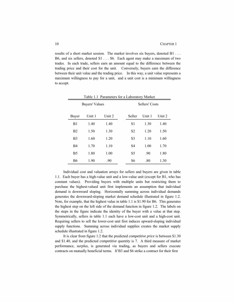
results of a short market session. The market involves six buyers, denoted B1 . . . B6, and six sellers, denoted S1 . . . S6. Each agent may make a maximum of two trades. In each trade, sellers earn an amount equal to the difference between the trading price and their cost for the unit. Conversely, buyers earn the difference between their unit value and the trading price. In this way, a unit value represents a maximum willingness to pay for a unit, and a unit cost is a minimum willingness to accept.

Individual cost and valuation arrays for sellers and buyers are given in table 1.1. Each buyer has a high-value unit and a low-value unit (except for B1, who has constant values). Providing buyers with multiple units but restricting them to purchase the highest-valued unit first implements an assumption that individual demand is downward sloping. Horizontally summing across individual demands generates the downward-sloping market demand schedule illustrated in figure 1.2. Note, for example, that the highest value in table 1.1 is $1.90 for B6. This generates the highest step on the left side of the demand function in figure 1.2. The labels on the steps in the figure indicate the identity of the buyer with a value at that step. Symmetrically, sellers in table 1.1 each have a low-cost unit and a high-cost unit. Requiring sellers to sell the lower-cost unit first induces upward-sloping individual supply functions. Summing across individual supplies creates the market supply schedule illustrated in figure 1.2. It is clear from figure 1.2 that the predicted competitive price is between $1.30 and $1.40, and the predicted competitive quantity is 7. A third measure of market performance, surplus, is generated via trading, as buyers and sellers execute contracts on mutually beneficial terms. If B3 and S6 strike a contract for their first

Table 1.1 Parameters for a Laboratory Market

Buyers' Values

Sellers' Costs

Buyer Unit 1 Unit 2 Seller Unit 1 Unit 2

B1 1.40 1.40 S1 1.30 1.40

B2 1.50 1.30 S2 1.20 1.50

B3 1.60 1.20 S3 1.10 1.60

B4 1.70 1.10 S4 1.00 1.70

B5 1.80 1.00 S5 .90 1.80

B6 1.90 .90 S6 .80 1.30

INTRODUCTION AND OVERVIEW 11

units, then the surplus created is $.80 ($1.60 – $.80). The maximum possible surplus that can be extracted from trade is $3.70, which is the area between the supply and demand curves to the left of their intersection. These predictions are summarized in the left-most column of table 1.2. Efficiency, measured as the percentage of the maximum possible surplus extracted, is shown in the fourth row of the table. Competitive price theory predicts (in the absence of externalities and other imperfections) that trading maximizes possible gains from exchange, and thus, predicted efficiency for the competitive theory is 100 percent.9 Finally, the available surplus could be distributed in a variety of ways, depending on the contracts made in the sequence of trades. Suppose B3 and S6 strike the contract as just mentioned for a price of $1.30. At this price, $.30 of the created surplus goes to B3 ($1.60 – $1.30), while $.50 of the surplus goes to S6 ($1.30 – $.80). The distribution of this surplus would be just reversed if the contract was struck at a price of $1.10. Under competitive conditions, the surplus should be distributed roughly equally among buyers and sellers in this design. If prices were exactly in the middle of the competitive range, then 50 percent of the surplus would go to the buyers and 50 percent to the sellers. As indicated by the “~” marks in the bottom two entries in the Perfect Competition

9 Some aspects of the efficiency concept are discussed in section 3.2 of chapter 3.

Figure 1.2 Supply and Demand Structure for a Market Experiment

12 CHAPTER 1

column, however, deviations from the 50/50 split are consistent with a competitive outcome, due to the range of competitive prices in this design. To evaluate the results of an experiment, it is useful to consider some alternative theories. If students in an economics class are given the value and cost information in table 1.1 (but not the representation in figure 1.2) and are asked to provide a theory that predicts the price outcomes for double-auction trading, they commonly suggest procedures that involve calculating means or medians of values and costs. If students are then shown figure 1.2 and asked to suggest alternatives to the theory of perfect competition, the suggestions are often couched in terms of maximization of one form or another. Perhaps the three most frequently suggested theories are (a) maximization of combined sellers' profits, (b) maximization of combined buyers' earnings, and (c) maximization of the number of units that can be traded at no loss to either party.10 The predictions of these three alternative theories are summarized in the three columns on the right side of table 1.2. Consider the predictions listed under the Monopoly column in the table. Assuming that units sell at a uniform price, the profit-maximizing monopoly price is $1.60, and four units will trade in a period. This yields a total revenue of $6.40 (four times $1.60). The least expensive way of producing four units is to use the “first units” of sellers S3-S6, for a total cost of $3.80 ($0.80 + $0.90 + $1.00 + $1.10). The resulting profit is the difference between revenue and cost, which is $2.60.11 Buyers' surplus at the monopoly price is only $0.60 ($0.30 for B6, $0.20 for B5, and $0.10 for B4). Total surplus is the sum of sellers' profits and buyers' surplus; this sum is $3.20, which is 87 percent of the maximum possible gains from trade ($3.70) that could be extracted from the market. Sellers will earn roughly 81 percent of that surplus (or the area between $1.60 and the supply curve for the first four units in figure 1.2).12 The symmetric predictions of buyer surplus maximization are summarized in the monopsony column of table 1.2. Finally, consider quantity maximization as a predictor. From a reexamination of table 1.1 it is clear that this design has the interesting feature that a maximum of twelve profitable trades can be made in a period, if all trades take

10 In our experience, economics students offer these theories more frequently than the (surplus-maximizing) model of perfect competition, which appears in all of their textbooks.

11 It can be verified that this is the monopoly price by constructing a marginal revenue curve. Alternatively, consider profits at nearby prices: Raising the price to $1.70 decreases sales to three units and profits to $2.40. Lowering the price to $1.50 increases sales to five units, but profits fall to $2.50. Other prices are even less profitable.

12 An even more profitable theory of seller profit maximization is that sellers perfectly price discriminate by selling one unit at $1.90, one unit at $1.80, etc. In this case, seven units trade, 100 percent efficiency is extracted, and all earnings go to sellers. A symmetric, cost-discrimination theory of buyer earnings maximization is also possible. These theories are left out of table 1.2 for ease of presentation.

INTRODUCTION AND OVERVIEW 13

place at different prices.13 In each trade, a buyer and seller will negotiate over the ten-cent difference between supply and demand steps, so there is no point prediction about the price and surplus distribution. Each trade generates a ten-cent surplus, so the total surplus is only $1.20, or about 32 percent of the maximum possible surplus. In order for twelve units to be traded, prices will be about as dispersed as individuals' values and costs, as indicated by the range of “.80 to 1.90” in the right-hand column of the table.

We conducted a short market session using twelve student participants and the parameters summarized in table 1.1.14 The session consisted of two “trading periods.” At the beginning of each period, the twelve participants were each privately assigned one of the cost or valuation schedules listed in table 1.1. Then they were given ten minutes to negotiate trades according to double-auction trading rules mentioned above: sellers could call out offer prices, which could be accepted by any buyer, and buyers could call out bid prices, which could be accepted by any seller. (The instructions used for this experiment are reproduced in appendix A1.1.) The transactions prices for the first period are listed below in temporal order, with prices in the competitive range underlined. 13 Let Sij denote the jth unit of seller Si, etc. Then twelve profitable trades can occur if they take place in the following order: S11 trades with B11, B21 with S12, S21 with B22, S22 with B31, S31 with B32, S32 with B41, S41 with B42, S42 with B51, S51 with B52, S52 with B61, S61 with B62, and finally S62 with B12.

14 Participants were fourth-year economics majors at the University of Virginia, and they were recruited from a small seminar class. None of the subjects had previously participated in a laboratory market. The session was conducted orally, with all prices recorded on the blackboard. Earnings were paid in cash at the end of two periods.

Table 1.2 Properties of Alternative Market Outcomes

Perfect Competition

Monopoly

Monopsony

Quantity Maximization

Price 1.30 to 1.40 1.60 1.10 .80 to 1.90

Quantity 7 4 4 12

Surplus 3.70 3.20 3.20 1.20

Efficiency 100% 87% 87% 32%

Buyers' Surplus ~50% 19% 81% –

Sellers' Surplus ~50% 81% 19% –

14 CHAPTER 1

Period 1: $1.60, 1.50, 1.50, 1.35, 1.25, 1.39, 1.40. Participants calculated their earnings at the end of the first period, and then the market was opened for a second period of trading, which only lasted seven minutes. The transactions prices for the second period are: Period 2: $1.35, 1.35, 1.40, 1.35, 1.40, 1.40, 1.35. Thus, by the second period, outcomes are entirely consistent with competitive predictions: All transactions were in the competitive price range, and seven units sold. The market was 100 percent efficient in both periods. These competitive results are typical of those obtained with the parameterization in figure 1.2. Notice that the number of traders was relatively small, and that no trader initially knew anything about supply and demand conditions for the market as a whole.15 1.4 Experimental Methods: Advantages and Limitations Each of the three literatures mentioned in section 1.2 has generated a body of findings using human subjects (usually college undergraduates) who make decisions in highly structured situations. The skeptical reader might question what can be learned about complex economic phenomena from behavior in these simple laboratory environments. Although this issue arises repeatedly in later chapters, it is useful to present a brief summary of the pros and cons of experimentation at this time. The chief advantages offered by laboratory methods in any science are replicability and control. Replicability refers to the capacity of other researchers to reproduce the experiment, and thereby verify the findings independently.16 To a degree, lack of replicability is a problem of any observational inquiry that is nonexperimental; data from naturally occurring processes are recorded in a unique and nonreplicated spatial and temporal background in which other unobserved factors are constantly changing.17 The problem is complicated in economics because

15 If the demand and supply functions are more asymmetric, convergence to a stationary pattern of behavior typically involves more than two periods. Chapter 3 considers some conditions under which convergence in double-auction markets is either slow or erratic.

16 This notion of replication should be distinguished from the conventional use of the term in econometrics. As Roth (1990) notes, the notion of replication in econometrics refers to the capacity to reproduce results with a given data set. In an experimental context, replication is the capacity to create an entirely new set of observations.

17 Laboratory observations, of course, also occur at spatially and temporally distinct locations, but laboratory procedures are implemented specifically to control for such effects. With careful attention, the

INTRODUCTION AND OVERVIEW 15

the collection and independent verification of economic data are very expensive. Moreover, the economics profession imposes little professional credibility on the data-collection process, so economic data are typically collected not by economists for scientific purposes, but by government employees or businessmen for other purposes. For this reason it is often difficult to verify the accuracy of field data.18 Better data from naturally occurring markets could be collected, and there is certainly a strong case to be made for improvements in this area. But relatively inexpensive, independently conducted laboratory investigations allow replication, which in turn provides professional incentives to collect relevant data carefully. Control is the capacity to manipulate laboratory conditions so that observed behavior can be used to evaluate alternative theories and policies. In natural markets, an absence of control is manifested in varying degrees. Distinguishing natural data may sometimes exist in principle, but the data are either not collected or collected too imprecisely to distinguish among alternative theories. In other instances, relevant data cannot be collected, because it is simply impossible to find economic situations that match the assumptions of the theory. An absence of control in natural contexts presents critical data problems in many areas of economic research. In individual decision theory, for example, one would be quite surprised to observe many instances outside the laboratory where individuals face questions that directly test the axioms of expected utility theory. The predictions of game theory are also frequently difficult to evaluate with natural data. Many game-theoretic models exhibit a multiplicity of equilibria. Game theorists frequently narrow the range of outcomes by dismissing some equilibria as being “unreasonable,” often on very subtle bases, such as the nature of beliefs about what would happen in contingencies that are never realized during the equilibrium play of the game (beliefs “off of the equilibrium path”). There is little hope that such issues can be evaluated with nonexperimental data. Perhaps more surprising is the lack of control over data from natural markets sufficient to test even basic predictions of neoclassical price theory. Consider, for example, the simple proposition that a market will generate efficient, competitive prices and quantities. Evaluation of this proposition requires price, quantity, and market efficiency data, given a particular set of market demand and supply curves. But neither supply nor demand may be directly observed with natural data. Sometimes cost data may be used to estimate supply, but the complexity of most markets forces some parameter measurements to be based on one or more convenient simplifications, such as log linearity or perfect product homogeneity,

experimenter can approximately duplicate a test environment in a subsequent trial.

18 The Washington Post (July 5, 1990, p. D1) summarized this consensus: “In studying government data, everyone from the National Academy of Sciences to the National Association of Business Economists has reached the same conclusion ─ there are serious problems regarding the accuracy and usefulness of the statistics.”

16 CHAPTER 1

which are violated in nonlaboratory markets, often to an unknown extent.19 Demand is even more difficult to observe, since there is nothing analogous to cost data for consumers. Although econometric methods may be used to estimate market supply and demand curves from transactions-price data, this estimation process typically rests on an assumption that prices are constantly near the equilibrium. (Then shifts in supply, holding demand constant, may be used to identify demand, and conversely for supply estimates.) Alternatively it is possible to estimate supply and demand without assuming that the market is in equilibrium, but in this case it is necessary to make specific assumptions about the nature of the disequilibrium. In either case, it is a questionable exercise to attempt to evaluate equilibrium tendencies in a market where supply and demand are estimated on the basis of specific assumptions about whether or how markets equilibrate. Thus, tests of market propositions with natural data are joint tests of a rather complicated set of primary and auxiliary hypotheses. Unless auxiliary hypotheses are valid, tests of primary hypotheses provide little indisputable information. On the one hand, negative results do not allow rejection of a theory. Evidence that seems to contradict the implications of a theory may arise when the theory is true, if a subsidiary hypothesis is false. On the other hand, even very supportive results may be misleading because a test may generate the “right” result, but for the wrong reason; the primary hypotheses may have no explanatory power, yet subsidiary hypotheses may be sufficiently incorrect to generate apparently supportive data. Laboratory methods allow a dramatic reduction in the number of auxiliary hypotheses involved in examining a primary hypothesis. For example, using the cost and value inducement procedure introduced by Chamberlin and Smith, a test of the capacity of a market to generate competitive price and quantity predictions can be conducted without assumptions about functional forms and product homogeneity that are typically needed to estimate competitive price predictions in a naturally occurring market. By inducing a controlled environment that is fully understood by the investigator, laboratory methods can be used to provide a minimal test of a theory. If the theory does not work under the controlled “best-shot” conditions of the laboratory, the obvious question is whether it will work well under any circumstances. Even given the shortcomings of nonexperimental data, critics are often skeptical about the value of laboratory methods in economics. Some immediate sources of skepticism are far less critical than they first appear. For example, one natural reservation is that relevant decision makers in the economy are more

19 Anyone who is familiar with predatory pricing cases, for example, knows the difficulties of measuring a concept as simple as average variable cost. Moreover, tests for predatory pricing (such as the Areeda/Turner test) are operationalized in average-cost rather than in more theoretically precise marginal-cost terms, because marginal-cost measures are too elusive.

INTRODUCTION AND OVERVIEW 17

sophisticated than undergraduates or MBA students who comprise most subject pools. This critique is more relevant for some types of experiments (e.g., studies of trading in futures markets) than for others (e.g., studies of consumer shopping behavior), but in any event, it is an argument about the choice of subjects rather than about the usefulness of experimentation. If the economic agents in relevant markets think differently from undergraduates, then the selection of subjects should reflect this. Notably, the behavior of decision makers recruited from naturally occurring markets has been examined in a variety of contexts, for example, Dyer, Kagel, and Levin (1989), Smith, Suchanek, and Williams (1988), Mestelman and Feeny (1988), and DeJong et. al (1988). Behavior of these decision makers has typically not differed from that exhibited by more standard (and far less costly) student subject pools. For example, Smith, Suchanek, Williams (1988) observed price “bubbles” and “crashes” in laboratory asset markets, with both student subjects and business and professional people.20 A second immediate reservation concerning the use of experiments is that the markets of primary interest to economists are complicated, while laboratory environments are often relatively simple. This objection, however, is as much a criticism of the theories as of the experiments. Granted, performance of a theory in a simple laboratory setting may not carry over to a more complex natural setting. If this is the case, and if the experiment is structured in a manner that is consistent with the relevant economic theory, then perhaps the theory has omitted some potentially important feature of the economy. On the other hand, if the theory fails to work in a simple experiment, then there is little reason to expect it to work in a more complicated natural world.21 It is imperative to add that experimentation is no panacea. Important issues in experimental design, administration, and interpretation bear continued scrutiny. For instance, although concerns regarding subject pool and environmental simplicity are not grounds for dismissing experimental methods out of hand, these issues do present prominent concerns. While available evidence suggests that the use of relevant professionals does not invariably affect performance, a number of studies do indicate that performance can vary with proxies for the aptitude of participants, such as the undergraduate institution (e.g., Davis and Holt, 1991) or using graduate instead of undergraduate students.22 For this reason, choosing a specific participant pool may be appropriate in some instances.

20 In some instances the use of “relevant professionals” impedes laboratory performance. Dyer, Kagel, and Levin (1989) and Burns (1985) find that relevant professionals involved in laboratory markets sometimes attempt to apply rules of thumb, which, while valuable for dealing with uncertainty in the parallel natural market, are meaningless guides in the laboratory. DeJong et al. (1988) report that businessmen need more instruction on the use of a computer keyboard.

21 This defense is well articulated by Plott (1982, 1989).

22 Ball and Cech (1991) provide a very extensive survey of subject-pool effects.

18 CHAPTER 1

Similarly, the relative simplicity of laboratory markets can be an important drawback if one's purpose is to make claims regarding the performance of natural markets. Economists in general are well acquainted with the pressures to “oversell” research results in an effort to attract funds from agencies interested in policy-relevant research. Experimental investigators are by no means immune to such temptations. It is all too easy, for instance, to give an investigation of a game-theoretic equilibrium concept the appearance of policy relevance by attaching catchy labels to the alternative decisions, and then interpreting the results in a broad policy context. But realistically, no variant of a prisoner's-dilemma experiment will provide much new information about industrial policy, regardless of how the decisions are labeled. Technical difficulties in establishing and controlling the laboratory environment also present important impediments to effective experimentation. This is particularly true when the purpose of the experiment is to elicit information about individual preferences (as opposed to evaluating the outcomes of group interactions given a set of induced preferences). The effectiveness of many macroeconomic policies, for example, depends on the recognition of intertemporal tradeoffs. Do people anticipate that tax cuts today will necessitate increases later, perhaps decades later? Do agents care about what happens to future generations? Do agents have a bequest motive? Although these are clearly behavioral questions, they may be very difficult to address in the laboratory. Most people may only consider questions regarding bequests seriously in their later years, and responses regarding intended behavior at other times may be poor predictors. Although elaborate schemes have been devised to address elicitation issues, it is probably fair to say that experimentalists have been much less successful with the elicitation of preferences than with their inducement. In addition, there are some ongoing questions about whether it is technically possible to induce critical components of some economic environments in the laboratory, for example, infinite horizons or risk aversion. Some very clever approaches to these problems will be discussed in later chapters. Overall, the advantages of experimentation are decisive. Experimental methods, however, complement rather than substitute for other empirical techniques. Moreover, in some contexts we can hope to learn relatively little from experimentation. It is important to keep the initial infatuation with the novelty of the technique from leading to the mindless application of experimental methods to every issue or model that appears in the journals. 1.5 Types of Experiments The “stick” of replicability forces those who conduct experiments to consider in detail the appropriate procedures for designing and administering experiments, as well as standards for evaluating them. Laboratory investigations can have a variety

INTRODUCTION AND OVERVIEW 19

of aims, however, and appropriate procedures depend on the kind of experiment being conducted. For this reason it is instructive to discuss several alternative objectives of experimentation: tests of behavioral hypotheses, sensitivity tests, and documentation of empirical regularities. This discussion is introductory. Chapter 9 contains a more thorough discussion of the relationship between economic experiments and tests of economic propositions. Tests of Behavioral Hypotheses Perhaps the most common use of experimental methods in economics is theory falsification. By constructing a laboratory environment that satisfies as many of the structural assumptions of a particular theory as possible, its behavioral implications can be given a best chance. Poor predictive power under such circumstances is particularly troubling for the theory's proponents. It is rarely a trivial task to construct idealized environments, that is, environments consistent with the structural assumptions of the relevant model. Indeed, this task is not likely to be accomplished in one iteration of experimentation. Despite the glamour of the much heralded “critical experiment,” such breakthroughs are rare. Rather, the process of empirical evaluation more often involves a continuing interaction between theorist and experimenter, and often addresses elements initially ignored in theory. For example, Chamberlin's demonstration that markets fail to generate competitive outcomes led Smith to consider the effects of trading rules on market performance, and ultimately led to the extensive consideration of important institutional factors that had been typically ignored by theorists. In this way, experiments foster development of a dialogue between the theorist and the empiricist, a dialogue that forces the theorist to specify models in terms of observable variables, and forces the data collector to be precise and clever in obtaining the desired control. Theory Stress Tests If the key behavioral assumptions of a theory are not rejected in a minimal laboratory environment, the logical next step is to begin bridging the gap between laboratory and naturally occurring markets. One approach to this problem involves examining the sensitivity of a theory to violations of “obviously unrealistic” simplifying assumptions. For example, even if theories of perfect competition and perfect contestability organize behavior in simple laboratory implementations, these theories would be of limited practical value if they were unable to accommodate finite numbers of agents or small, positive entry costs. By examining laboratory markets with progressively fewer sellers, or with positive (and increasing) entry costs, the robustness of each theory to its simplifying assumptions can be evaluated.

20 CHAPTER 1

Systematic stress-testing a theory in this manner is usually not possible with an analysis of nonexperimental data.23 Another immediate application of a theory stress test involves information. Most game theories postulate complete information, or incomplete information in a carefully limited dimension. But in some applications (e.g., industrial organization) game theory is being used too simplistically if the accuracy of its predictions is sensitive to small amounts of uncertainty about parameters of the market structure. There is some evidence that this is not the case, that is, that the concept of a noncooperative (Nash) equilibrium sometimes has more predictive power when subjects are given no information about others' payoff functions (Fouraker and Siegel, 1963, and Dolbear et al., 1968). This is because subjects do not have to calculate the noncooperative equilibrium strategies in the way that a theorist would; all they have to do is respond optimally to the empirical distribution of others' decisions observed in previous plays of the game. Searching for Empirical Regularities A particularly valuable type of empirical research is the documentation of surprising regularities in relationships between observed economic variables. For example, the negative effect of cumulative production experience on unit costs has led to a large literature on “learning curves.” Roth (1986) notes that experimentation can also be used to discover and document such “stylized facts.” This search is facilitated in laboratory markets in which there is little or no measurement error and in which the basic underlying demand, supply, and informational conditions are known by the experimenter. It would be difficult to conclude that prices in a particular industry are above competitive levels, for example, if marginal costs or secret discounts cannot be measured very well, as is usually the case. Anyone who has followed an empirical debate in the economics literature (for example, the concentration-profits debate in industrial organization) can appreciate the attractiveness of learning something from market experiments, even if the issues considered are more limited in scope. 1.6 Some Procedural and Design Considerations The diversity of research objectives and designs complicates identification of a single set of acceptable laboratory procedures. Consequently, both desirable and undesirable procedures will be discussed in various portions of the text, and specific examples and applications will be given in the chapter appendices. However, there

23 This “stress test” terminology is due to Ledyard (1990).

INTRODUCTION AND OVERVIEW 21

are some general design and procedural considerations common to most laboratory investigations, and it is instructive to review them at this time. For clarity, this discussion will be presented primarily in terms of market experiments. In general, the experimental design should enable the researcher to utilize the main advantages of experimentation that were discussed above: replicability and control. Although a classification of design considerations is, to some extent, a matter of taste, we find the following categories to be useful: procedural regularity, motivation, unbiasedness, calibration, and design parallelism. Procedural regularity involves following a routine that can be replicated. Motivation, unbiasedness, and calibration are important features of control that will be explained below. Design

parallelism pertains to links between an experimental setting and a naturally occurring economic process. These design criteria will be discussed in a general manner here; specific practical implications of some of these criteria are incorporated into a detailed list of suggestions for conducting a market experiment in appendix A1.2. Prior to proceeding, it is convenient to introduce some terminology. No standard conventions have yet arisen for referring to the components of an experiment, so for purposes of clarity we will adopt the following terminology: session: a sequence of periods, games, or other decision tasks

involving the same group of subjects on the same day cohort: a group of subjects that participated in a session treatment: a unique environment or configuration of treatment

variables, i.e., of information, experience, incentives, and rules

cell: a set of sessions with the same experimental treatment conditions

experiment design: a specification of sessions in one or more cells to evaluate the propositions of interest

experiment: the collection of sessions in one or more related cells The reader should be warned that some of these terms are often used differently in the literature. In particular, it is common to use the word “experiment” to indicate what we will call a “session.” Our definition follows Roth (1990), who argues that the interaction of a group of subjects in a single meeting should be called a “session,” and that the word “experiment” should be reserved for a collection of sessions designed to evaluate one or more related economic propositions. By this definition an experiment is usually, but not always, the evidence reported in a single paper.24

24 We will, however, continue to use “experiment” in a loose manner in instructions for subjects.

22 CHAPTER 1

Finally, most experimental sessions involve repeated decisions, and some terms are needed to identify separate decision units. Appropriate terminology depends on the type of experiment: A decision unit will be referred to as a trial, when discussing individual decision-making experiments, as a game when discussing games, and as a trading period when discussing market experiments. Procedural Regularity The professional credibility that an experimenter places on data collected is critical to the usefulness of experiments. It is imperative that others can and do replicate laboratory results, and that the researcher feel the pressure of potential replication when conducting and reporting results. To facilitate replication, it is important that the procedures and environment be standardized so that only the treatment variables are adjusted. Moreover, it is important that these procedures (and particularly instructions) be carefully documented. In general, the guiding

principle for standardizing and reporting procedures is to permit a replication that

the researcher and outside observers would accept as being valid. The researcher should adopt and report standard practices pertaining to the following:25 instructions illustrative examples and tests of understanding (which should be included

in the instructions) criteria for answering questions (e.g., no information beyond instructions) the nature of monetary or other rewards the presence of “trial” or practice periods with no rewards the subject pool and the method of recruiting subjects the number and experience levels of subjects procedures for matching subjects and roles the location, approximate dates, and duration of experimental sessions the physical environment, the use of laboratory assistants, special devices, and computerization any intentional deception of subjects procedural irregularities in specific sessions that require interpretation Even if journal space requirements preclude the publication of instructions, work sheets, and data, the researcher should make this information available to journal referees and others who may wish to review and evaluate the research.

25 This list approximately corresponds to Palfrey and Porter's (1991) list in “Guidelines for Submissions of Experimental Manuscripts.”

INTRODUCTION AND OVERVIEW 23

The use of computers has done much to strengthen standards of replicability in economics.26 The presentation of the instructions and the experimental environment via visually isolated computer terminals increases standardization and control within an experiment and decreases the effort involved in replication with different groups of subjects. Moreover, some procedural tasks that involve a lot of interaction or privacy are much easier to implement via computer, and computerization often enables the researcher to obtain more observations within a session by economizing on the time devoted to record keeping and message delivery.27 Importantly, however, computers are not necessary to conduct most experiments. Even with extensive access to computers, some noncomputerized procedures retain their usefulness. The physical act of throwing dice, for example, may more convincingly generate random numbers than computer routines if subjects suspect deception or if payoffs are unusually large. Similarly, even when instructions are presented via computer, we generally prefer to have an experimenter read instructions aloud as the subjects follow on their screens. This increases common knowledge, that is, everyone knows that everyone else knows certain aspects of the procedures and payoffs. Reading along also prevents some subjects from finishing ahead of others and becoming bored. A final issue in procedural matters regards the creation and maintenance of a subject pool. Although rarely discussed, the manner in which subjects are recruited, instructed, and paid can importantly affect outcomes. Behavior in the laboratory may be colored by contacts the students have with each other outside the laboratory; for example, in experiments involving deception or cooperation, friends may behave differently from anonymous participants. Problems of this type may be particularly pronounced in some professional schools and European university systems, where all students in the same year take the same courses. Potential problems may be avoided by recruiting participants for a given session from multiple classes (years). For similar reasons, an experimenter may wish to avoid being present in sessions that involve subjects who are currently enrolled in one of his or her courses. Such students may alter their choices in light of what they think their professor wants to see. The researcher should also be careful to avoid deceiving participants. Most economists are very concerned about developing and maintaining a reputation among the student population for honesty in order to ensure that subject actions are

26 At present there are some two dozen computerized economics laboratories in the United States, as well as several in Europe.

27 The effects of computerization in the context of the double auction are discussed in chapter 3, section 3.3. Also, one of the advantages of computerization lies in the way instructions can be presented. Instructions for a computerized implementation of a posted-offer auction are presented in appendix 4.2 to chapter 4.

24 CHAPTER 1

motivated by the induced monetary rewards rather than by psychological reactions to suspected manipulation. Subjects may suspect deception if it is present. Moreover, even if subjects fail to detect deception within a session, it may jeopardize future experiments if the subjects ever find out that they were deceived and report this information to their friends.28 Another important aspect of maintaining a subject pool is the development of a system for recording subjects' history of participation. This is particularly important at universities where experiments are done by a number of different researchers. A common record of names and participation dates allows each experimenter to be more certain that a new subject is really inexperienced with the institution being used. Similarly, in sessions where experience is desired, a good record-keeping system makes it possible to control the repeated use of the same subjects in multiple “experienced” sessions. Motivation In designing an experiment, it is critical that participants receive salient rewards that correspond to the incentives assumed in the relevant theory or application. Saliency simply means that changes in decisions have a prominent effect on rewards. Saliency requires (1) that the subjects perceive the relationship between decisions made and payoff outcomes, and (2) that the induced rewards are high enough to matter in the sense that they dominate subjective costs of making decisions and trades. For example, consider a competitive quantity prediction that requires the trade of a unit worth $1.40 to a buyer, but which costs a seller $1.30. This trade will not be completed, and the competitive quantity prediction will “fail,” if the joint costs of negotiating the contract exceed $.10. One can never be assured, a priori, that rewards are adequate without considering the context of a particular experiment. On the one hand, participants will try to “do well” in many instances by maximizing even purely hypothetical payment amounts. On the other hand, inconsistent or variable behavior is not necessarily a signal of insufficient monetary incentives. No amount of money can motivate subjects to perform a calculation beyond their intellectual capacities, any more than generous bonuses would transform most of us into professional athletes.29 It has been fairly well established, however, that providing payments to subjects

28 Many economists believe that deception is highly undesirable in economics experiments, and for this reason, they argue that the results of experiments using deceptive procedures should not be published. Deceptive procedures are more common and perhaps less objectionable in other disciplines (e.g., psychology).

29 Vernon Smith made a similar point in a different context in an oral presentation at the Economic Science Association Meetings, October 1988.

INTRODUCTION AND OVERVIEW 25

tends to reduce performance variability.30 For this reason, economics experiments almost always involve nonhypothetical payments. Also, as a general matter, rewards are monetary. Monetary payoffs minimize concerns regarding the effects of heterogeneous individual attitudes toward the reward medium. Denominating rewards in terms of physical commodities such as coffee cups or chocolate bars may come at the cost of some loss in control, since participants may privately value the physical commodities very differently. Monetary payoffs are also highly divisible and have the advantage of nonsatiation; it is somewhat less problematic to assume that participants do not become “full” of money than, say, chocolate bars. In many contexts, inducing a sufficient motivation for marginal actions will require a substantial variation in earnings across participants, even if all participants make careful decisions. High-cost sellers in a market, for example, will tend to earn less than low-cost sellers, regardless of their decisions. If possible, average rewards should be set high enough to offset the opportunity cost of time for all participants. This opportunity cost will depend on the subject pool; it will be higher for professionals than for student subjects. If there are several alternative theories or hypotheses being considered, then the earnings levels should be adequate for motivational purposes at each of the alternative outcomes under consideration. For example, if sellers' earnings are zero at a competitive equilibrium, then competitive pricing behavior may not be observed, since zero earnings may result in erratic behavior. In some experiments, subjects' earnings are denominated in a laboratory currency, for example, tokens or francs, and later converted into cash. A very low conversion rate (e.g., 100 laboratory “francs” per penny earned) can create a fine price grid to more nearly approximate theoretical results of continuous models. A coarse price grid in oligopoly games, for example, can introduce a number of additional, unwelcome equilibria. A second advantage of using a laboratory currency “filter” arises in situations where the experimenter wishes to minimize interpersonal payoff comparisons by giving subjects different conversion ratios that are private information. Procedures of this sort have been used in bargaining experiments. A laboratory currency may also be used to control the location of focal payoff points when payoff levels are of some concern. The effects of earnings levels on the absolute payoff level could be controlled, for example, by conducting treatments in the same design, but under different franc/dollar conversion rates. The

30 In the absence of financial incentives, it is more common to observe occasional large and nonsystematic deviations in behavior from the norm. In addition, the relevant economic model often yields better predictions when sufficient financial motivation is provided. For example, Siegel and Goldstein (1959) showed that an increase in the reward level resulted in an increase in the proportion of rational, maximizing choices in a forecasting experiment. This experiment is discussed in chapter 2.

26 CHAPTER 1

denomination of payoffs in lab dollars could also control for differences in focal points in sessions conducted in different countries with different currencies. Some experimentalists further maintain that a currency filter can increase incentives; for example, subjects may make an effort to earn 100 francs, even if they would scoff at the monetary equivalent of, say, one penny. We find this money-illusion argument less persuasive. Many tourists in a foreign country for the first time return with stories about spending thousands of pesos, or whatever, and not worrying about the real cost of goods. It is possible that the use of a laboratory currency could similarly mask or even dilute financial incentives. Moreover, even if laboratory payoffs do create a monetary illusion, they could also create an artificial “game-board” sense of speculative competitiveness. For these reasons, it is probably prudent to denominate laboratory earnings in cash, unless the researcher has a specific design motivation for using a laboratory currency. Three additional comments regarding motivation bear brief mention. First, it is a fairly standard practice to pay participants an appearance fee in addition to their earnings in the course of the experiment. Payment of a preannounced fee facilitates recruiting of subjects, establishes credibility, and perhaps provides some incentive for participants to pay attention to instructions. Second, it is usually important for the experimenter to be specific about all aspects of the experiment in order to control the motivation. For example, the failure to provide information about the duration or number of periods in a session may affect subjects' perceptions of the incentives to collude in an unknown and uncontrolled manner. The third point is a qualification of the second. There is a risk of losing control over incentives if subjects are given complete information about others' money payoffs. With complete information, envy and benevolence are more likely, which is a problem if the theoretical model stipulates that agents maximize their own payoffs. Smith (1982) includes privacy (only knowing one's own payoff function) in a list of sufficient conditions for a valid microeconomics experiment. Privacy is appropriate for some purposes, such as tests of theories that specify privacy or stress tests of those that do not. On the other hand, privacy may not be appropriate for experiments motivated by a game-theoretic model that specifies complete information about the game structure.31 Unbiasedness Experiments should be conducted in a manner that does not lead participants to perceive any particular behavioral pattern as being correct or expected, unless explicit suggestion is a treatment variable. The possibility of replication should provide incentives sufficient to deter egregious attempts at distorting participant

31 Smith (1982) contains a classic discussion of motivation, which is based on formal definitions of nonsatiation, saliency, and privacy.

INTRODUCTION AND OVERVIEW 27

behavior. We mention the issue of biasedness, however, not to warn researchers away from patently suggestive behavior, but rather to note how careful even the most well-intentioned researcher must be to avoid subtle behavioral suggestions. Unlike other observational laboratory data (say atomic particles), human participants can be eager to do what the researcher desires and can respond to surprisingly subtle indications that they are doing “well.” If an experiment is conducted by hand, it is sometimes useful to have the experiment administrator be unaware of the theoretical predictions in a particular design. In a laboratory market session, for example, this can be done by adding a parameter-disguising constant to all values and costs, which shifts supply and demand vertically by the same distance, without changing the essential structure of the market. Altering the shift parameter with each session makes it possible for an experiment monitor to be unaware of the equilibrium price. These alterations also reduce the chance that ex post discussions among students will affect behavior in subsequent sessions. Some researchers believe that sessions should be conducted by assistants who do not know the purpose of the experiment, that is, in a “double-blind” setting. Our own feeling is that the researcher has the strongest incentive and ability to spot procedural problems, and therefore we prefer to be present during a session. But subjects in some types of experiments, especially those involving fairness issues, may be influenced by the fact that they are being observed by third parties. In such situations, it may be best for the researcher to be unobtrusive or unobserved. Another possible source of bias is the terminology used to explain the incentives. The trade of abstract commodities, as opposed to “pollution permits” or “failing firms,” may prevent unobserved personal preferences or aversions for particular goods from influencing results. Certain economic or market terms may also suggest particular types of behavior, for example, “cartel” or “conspiracy.” For these reasons, it is usually considered a good practice to avoid references to any particular good. There is, however, a tradeoff to be made here. Although simple tests of game-theoretic concepts can and should be conducted without giving economic names to the decision variables, the use of market terminology in other, more complicated trading institutions is valuable in communicating the payoff structure effectively. For example, although is possible to conduct one of Smith's double-auction market experiments without ever using words such as “buyer,” “seller,” or “price,” it would be very difficult to explain the structure to the subjects. (If you are not convinced, try it! Revise the double-auction instructions in appendix A1.1 so that they are entirely neutral with respect to market terminology.) One should use common sense in evaluating the tradeoff between providing enough of an economic context to explain the incentive structure and not providing suggestive terminology. It is worthwhile to spend a lot of time working on instructions; the safest procedure is to begin with standard, often-used instructions, and to modify them for the purpose at hand. Pilot experiments and individual “debriefing” sessions can be useful in spotting problems with the wording. For

28 CHAPTER 1

example, one of the authors once had a subject tell him that the word “oligopoly” on a receipt form “gave away” the purpose of the experiment, since the subject remembered from his introductory economics class that oligopolists are supposed to collude. This subject was unusually successful at colluding. As a result, all previously collected data were discarded, and the receipt form was changed. Calibration Experiments also need to be designed with an eye to the generated data. Calibration involves the establishment of a clear basis of comparison. Suppose, for example, that the hypothesis being investigated is that competitive behavior is altered by a treatment, say, the consolidation of market power in the hands of a few sellers. In this case, it is desirable to begin with a “baseline” condition in which competitive outcomes are generated in the absence of market power. A related aspect of calibration is the use of a design in which the predictions of alternative theories are cleanly separated. This aspect is important because the process of evaluating a behavioral theory comes through falsification rather than validation, and falsification is more convincing if there is a reasonable alternative that is not falsified. To make this discussion concrete, consider an evaluation of data that could be generated with the experimental market design in figure 1.2. Suppose that nine independent sessions (with different cohorts of subjects) have been conducted, each lasting for the same number of trading periods. Suppose further that we are concerned about evaluating the tendency for this market to generate predicted competitive prices (between $1.30 and $1.40). One way to analyze the results would be to take a single price measure from each session, such as the average final-period price. Admittedly, such a procedure discards much of the relevant data, but its simplicity makes it a useful expositional device. Also, the consequent observations have the advantage of statistical independence, since each session is done with a different group of subjects.32 Consider now some possible mean-price outcomes. Suppose first that prices deviated rather substantially and uniformly from the competitive prediction. For example, assume that the average of the nine price observations is $1.60, with a standard deviation (of the final-period mean prices) of $0.20. In this case, the null hypothesis of the competitive price prediction could be rejected at normal levels of

32 More sophisticated econometric techniques may be worthwhile if the results are not immediately apparent. Such techniques would involve the specification of the structure of the error terms in the process that generates transactions price data. The simple procedure used in the text is less powerful but avoids auxiliary assumptions.

INTRODUCTION AND OVERVIEW 29

significance.33 Now consider what happens when prices are closer to the competitive prediction. For example, suppose the mean of the nine observations was $1.45, with the same $.20 standard deviation. The null hypothesis of the competitive prediction could no longer be rejected at any conventional level of significance.34 But neither could it be accepted. In fact, we would be unable to make an affirmative statistical claim about the competitive prediction even if the mean price was closer to the competitive range. Rather, affirmative claims are limited to nonquantitative observations that prices “appear” to conform to the competitive prediction. This is the process (and problem) of falsification; we can sometimes determine when data do not support a theory, but it is far more difficult to conclude that evidence actually supports a theory. We avoid the philosophical issue of what is ultimately necessary for empirical verification of a theory. However, more convincing claims can be made if the data allow falsification of rival theories. For example, consider what could be said if the mean of the nine price observations was $1.35, with a $.20 standard deviation, in light of the monopoly or monopsony predictions listed in table 1.2. Although these observations cannot directly allow acceptance of the hypothesis that prices are competitive, the competitive-price hypothesis cannot be rejected, and the alternative hypotheses that prices are at the collusive level for either buyers or sellers can be rejected at standard significance levels. This is the issue of calibration. Theories are much more meaningfully evaluated in light of alternatives. Rejection of reasonable alternatives strengthens a failure to reject the maintained hypothesis. Conversely, a theory that organizes some aspects of the data well should not be discarded until a better alternative is found. Behavioral “noise” is inevitable. For example, although prices clustered about the competitive prediction in the two periods of the market session discussed in section 1.3, they were not uniformly confined within the bounds of the competitive price range. In fact, it is quite reasonable to suspect that some residual price variability would remain, even after a relatively large number of trading periods with the same traders. In light of this behavioral noise, two points need to be made. The first is a design issue. Careful experimental design requires more than merely identifying alternative predictions. The behavioral consequences of rival predictions should further be sufficiently distinct to be readily differentiated from inherent performance variability. For example, an alteration in the figure 1.2 design that made the demand curve much more elastic would make the behavioral distinction between cooperative and competitive behavior much more difficult, since the price consequences of these two alternatives would be much closer.

33 For example, a t-test statistic for the null hypothesis that observed prices are not significantly different from the competitive prediction would be 3, or [$1.60 – $1.40] / [.20 / 9]. Nonparametric tests are discussed in chapter 9.

34 The t-test statistic for the null examined in the previous footnote would be .75.

30 CHAPTER 1

The second issue has to do with anticipated performance variability that is outside the domain of the theory. Although some behavioral variability is effectively irreducible noise, there exist other theoretically irrelevant factors that quite regularly affect performance, such as experience with the experimental environment, group effects, and the order in which treatments are presented. To draw legitimate statistical claims, it is important to control for these anticipated sources of variability. Blocking, or systematic pairing of observations, may be used to neutralize the effects of such nuisance variables. Consider, for example, a market experiment designed to evaluate the effects of communication among sellers on pricing. The experiment contains two treatments: A (no-communication) and B (communication). If it turns out that communication tends to produce higher, collusive prices, it would also not be surprising to observe a sequencing, or order-of-treatment, effect. In a given session, we might expect to see higher prices in no-communication treatment A when it follows communication treatment B than when it precedes B. Sometimes the economics of the problem suggests a particular sequence. For example, it is often reasonable for a status quo treatment to precede a treatment that implements a possible alternative policy. When the economics of the situation does not require a particular sequence, it may be advisable to reverse the order of the treatments in every other session to control for sequence effects. Another way to avoid sequence effects would be to have only one treatment per session, but this necessitates a large number of sessions if there is considerable variability from one group of subjects to another. To clarify this point, suppose that six sessions using the A and B treatments are conducted, and that the sequence is alternated in every other session. Sessions in figure 1.3 are denoted as separate rows. In each row, the average price for each treatment is denoted with an A or a B, along a horizontal scale where prices increase with rightward movements. There is a clear treatment effect; in each session, price is higher for treatment B. But group effects are such that there is very little correlation between treatment and average price in the aggregate. Very little could have been concluded if the data in figure 1.3 had been generated from twelve independent sessions; both A and B observations tend to cluster about the vertical bar printed in the center of the graph. (Look in particular at the bottom row.) But consideration of the data in figure 1.3 as paired treatments allows one to reject the hypothesis of no treatment effect with a very high degree of confidence, with at least the same confidence that one can reject the hypothesis that a coin is fair after observing six heads in a row. In this context, blocking allows one to control for sequence and subject-group effects at the same time.35 The example in figure 1.3 also illustrates the notion that the structure of the experimental design (treatment cells, blocking, and numbers of trails) should

35 One potential disadvantage of using multiple treatments per session is that the amount of time available with each treatment is reduced. This can be a problem if adjustment to equilibrium is slow or erratic.

INTRODUCTION AND OVERVIEW 31

be planned with a consideration for the subsequent statistical analysis of the hypotheses of interest. This is rarely done by experimental economists, as noted by Hinkelmann (1990).

Sometimes the number of things that can be systematically blocked is unreasonably large and the alternative configurations can be selected randomly, in a randomized

block. For example, in an experiment with three buyers and one seller, there are twenty-four ways in which the order of subject arrival times can be related to the four role assignments. It would not be advisable to let the first person to arrive always have the monopoly role, since early arrival may be correlated with some unobserved characteristic of importance. A complete block would require twenty-four sessions, and a random assignment method is a simpler way to avoid systematic biases.36 Design Parallelism As a final design issue, we consider the extent to which experiments should be constructed to resemble naturally occurring economic situations. The term design

parallelism is used here to indicate closeness to natural situations rather than

36 We will say more about the relationship between experimental design and statistical analysis of data in chapter 9.

Session Lower Prices Higher Prices

1 A B

2 A B

3 A B

4 AB

5 A B

6 A B

1-6 A BA BAB A B A AB B Figure 1.3 Hypothetical Data from a Blocked Design

32 CHAPTER 1

closeness to the theories that economists have devised.37 Given the relative simplicity of laboratory environments, nonexperimentalists tend to be skeptical, and experimentalists should be cautious of claims about behavior in natural markets. Nevertheless, as a general matter, the experimenter should strive for parsimony. Recall that theory falsification is a prominent goal of experimental analysis. Such tests require specification of a laboratory environment that satisfies the conditions of the theory, rather than the conditions of a natural market. Increasing design parallelism by adding complexity to an experiment is seductively easy, but it often results in situations that are difficult to analyze in theory and difficult for subjects to comprehend quickly. The process of theory falsification in an idealized environment is not devoid of policy relevance. Although simple experiments will not predict the effects of a particular theory or policy remedy in richer environments, such experiments can provide a reasonable amount of evidence about whether policy proposals will have desired effects. For example, Isaac and Smith (1985) conducted a series of sessions with a proposed antipredation rule that prohibits a temporary price reduction by a dominant firm in response to entry; these sessions exhibited higher prices and lower efficiencies than were observed in comparable “unprotected” markets, conducted without the rule. These results make the regulatory “cure” highly suspect, for it harms performance even under the best of circumstances. In general, if the behavioral assumptions of a theory fail under simple conditions, the burden of explanation should be shifted to the advocates of the related policy. Maximum parsimony is not always desirable, however. Adding complexity is justifiable when attempting to make positive claims about a theory as part of the stress-testing process. The likelihood that a theory works in the natural world increases as the theory outperforms rival theories in increasingly complex experimental environments. In fact, it would seem logical to follow a laboratory study with a field experiment, that is, a test in a restricted natural setting. Field experiments are usually expensive, and as a consequence they are rare. One important issue in design parallelism is the appropriate amount of information to give subjects. For example, a minimal test of the behavioral assumptions of an oligopoly or game theory should reproduce the informational environment that is assumed in the theory, even though this may require much more precise information than is typically possessed by firms in industrial markets. On the other hand, experiments in which traders do not know each other's costs and values, such as Smith's (1962) initial market experiments, can be appropriately viewed both as sensitivity tests and as efforts to discover stylized facts in “realistic”

37 Smith (1982) used the term parallelism to mean transferability, i.e., that the results of the experiment will carry over to the corresponding nonexperimental setting. We use the term design parallelism to emphasize parallelism in the structure of the two settings, as opposed to parallelism in behavior.

INTRODUCTION AND OVERVIEW 33

environments. Therefore, the degree of design parallelism depends on the purpose of the experiment. Summary Although the discussion above may appear somewhat abstract, it is important to emphasize that it has is a very practical side. Those familiar with experimental methods simply will not take the results of an experiment seriously unless it satisfies some basic procedural standards. The most common “fatal errors” made by inexperienced researchers are:

failure to use complete and unbiased instructions failure to use salient financial rewards failure to include a baseline control treatment that calibrates results failure to restrict focus on a few treatments of interest that do not

change too many things at once failure to choose the degree of institutional complexity appropriate to

the problem being investigated

Any one of these failures pretty much renders results meaningless, even if the experiment is otherwise carefully conceived and reported. Finally, although these mistakes are readily spotted by the critic after the experiment is conducted, they can only be corrected before collecting data. A little extra planning and reflection prior to conducting an experiment can save many headaches. 1.7 Laboratory Trading Institutions Economists have traditionally viewed economic problems almost exclusively in terms of structural characteristics, such as the number of agents, their endowments, initial information, preferences, costs, and productive technologies. These structural characteristics, which must be induced in an experiment, are often referred to as the environment. The discovery of the behavioral importance of trading rules by Smith and others has led economists to reconsider the importance of institutions. In a loose sense, a market institution specifies the rules that govern the economic interaction: the nature and timing of messages and decisions, and the mapping from these messages and decisions to the traders' monetary earnings. Adding a specification of a trading institution to the analysis of an economic problem is consistent with the analytic approach taken by game theorists: both the game theorist and the experimentalist will assert that a full articulation of the problem's institutional and environmental components is necessary. The game theorist, however, uses somewhat different terminology. The articulation of a

34 CHAPTER 1

problem for the game theorist requires identification of each of the components of an extensive-form game that maps vectors of feasible strategies into utility “payoffs” for each player. Relevant components are comprised of a series of factors, which include the number of players, their payoff functions, and their knowledge (information sets).38 There is no simple correspondence between the game-theoretic and experimental terminology. For example, some payoff-relevant factors, such as commissions and transactions taxes, can be considered to be components of the trading institution. Other payoff-relevant factors, such as values or costs, define components of the environment. Each terminology has its benefits, and at various points each will be used.39 Regardless of the type of experiment or the focus of investigation, institutional rules and other environmental features must be specified. Most advanced theory texts do not pay much attention to institutional rules. For example, at the outset of a typical text, a tatonnement mechanism with its famous hypothetical auctioneer may be presented to justify price-taking competitive behavior. In a tatonnement mechanism, an auctioneer calls out a series of prices. Each agent responds to the announcements by truthfully indicating a quantity that the agent desires to purchase or sell at the price under consideration. In this sense, traders are “price takers.” A competitive, binding allocation occurs when quantity supplied equals quantity demanded.40 Competitive outcomes are assumed in the typical microeconomics text, at least until a chapter on imperfect competition that is likely to motivate noncompetitive outcomes with other institutions, such as the Cournot quantity-choice model, which (strictly speaking) rarely exists in naturally occurring markets.41 This neglect of institutional detail is unfortunate, since seemingly small alterations in the laboratory trading rules can have large effects, both on game-theoretic predictions and on observed behavior. Therefore, issues of institutional design are central in experimental economics. Experimentalists tend to classify experiments by both the institution and the subfield of economics that provides the research hypotheses. These two dimensions are closely related in practice. For example, Smith's double auctions are commonly used in the study of financial markets. Institutions with publicly posted list prices are commonly used in the analysis of retail markets with many small buyers. The organization of this book, therefore, is largely determined by the sequence of institutions considered. For this reason, a description of the commonly used

38 These terms are discussed in detail in chapter 2.

39 The terminology of the experimentalist has the advantage of forcing consideration of the manipulable components of an economic process even in instances where the structure of the game is too complicated to allow game-theoretic equilibrium analysis.

40 Price vectors, rather than single prices, are called out by the auctioneer in a multimarket setting.

41 The Cournot institution is discussed below.

INTRODUCTION AND OVERVIEW 35

laboratory institutions will provide a useful overview of the remainder of the book. It is also important to see how different institutions are related, since the intuition gained by observing trading in one institution can help one understand behavior in closely related contexts. The essential differences between the initially bewildering array of laboratory institutions to be encountered are listed in tables 1.3 and 1.4. The tables are distinguished by the timing of decisions. Simpler environments, where decisions are made independently (and in this sense simultaneously), are summarized in table 1.3. Table 1.4 summarizes more complex institutions where decisions are made sequentially, and in real time. In each table, the name of the institution is listed in the left column. The second column indicates the numbers of sellers and buyers, where a dash corresponds to any integer, and the special cases of one seller or one buyer are indicated with the number 1. The parenthetical notation in the second column indicates the number of units to be sold in auctions with an exogenously fixed supply. The third column shows whether buyers or sellers send price messages, which are called “bids” for buyers or “offers” or “asking prices” for sellers. The fourth column indicates whether messages are made simultaneously or sequentially. The final column, on the right side of the table, shows who responds to price proposals and how contracts are confirmed. The remainder of this section summarizes principal characteristics of these trading institutions. The discussion is divided into two subsections; simultaneous-decision institutions are considered first, followed by discussion of sequential-decision institutions. Institutions Involving Simultaneous Decisions It is natural to begin this discussion with the simple quantity-choice framework first articulated by Cournot (1838), because much of oligopoly theory is formulated in terms of this institution. In the Cournot institution, seller subjects select quantities simultaneously, and then each seller is told the aggregate quantity selected by all sellers. This market quantity determines price according to a simulated-buyer inverse demand schedule, which can be given to subjects in tabular form. Subjects use their own cost information to calculate their money profits. Subjects may or may not have complete information about other sellers' costs. As summarized in the first row of table 1.3, there can be any number of buyers and sellers, and no one sends price messages, since price is endogenous.42 An important disadvantage of this Cournot (posted quantity) institution is that critical behavioral assumptions are built into it; the implicit assumption is that, after output quantities are produced,

42 The Cournot institution has been used in experiments by Carlson (1967), Holt (1985), Holt and Villamil (1986), Welford (1990), and others.

36 CHAPTER 1

competition will drive price down (up) to the level at which there is no excess supply (demand).

The most prominent alternative to the Cournot model of quantity competition is the Bertrand (1883) model of price competition. An important implication of the Bertrand model is that price competition can lead to competitive outcomes, even in highly concentrated markets. Given a homogeneous product, excess capacity, and

Table 1.3 Trading Institutions with Simultaneous Decisions

#Sellers/#Buyers

(# units)

Who Proposes

Prices

Decisions and

Timing

How Contracts Confirmed

Cournot (quantity choice)

- / - price is endogenous

quantities posted simultaneously

simulated buyers

Posted Offer Auction

- / - sellers offers posted simultaneously

buyers shop in sequence

Ultimatum Bargaining (offer version)

1/1 seller seller makes single offer on 1 unit

buyer accepts or rejects

Posted Bid Auction

- / - buyers bids posted simultaneously

sellers shop in sequence

Discriminative Auction

1 / - (N units)

buyers bids posted simultaneously

highest N bidders pay own bids

1st Price Sealed-Bid Auction

1 / - (1 unit)

buyers bids posted simultaneously

high bidder pays own

“1st” price

Competitive Sealed-Bid Auction

1 / - (N units)

buyers bids posted simultaneously

highest N bidders pay N+1st price

Second Price Sealed-Bid Auction

1 / - (1 unit)

buyers bids posted simultaneously

highest bidder pays 2nd

price

Clearinghouse Auction

- / - buyers and sellers

bids and offers posted

simultaneously

intersection of bid and

offer arrays

INTRODUCTION AND OVERVIEW 37

simultaneous price postings, this result follows, since each seller always has an incentive to undercut any common supracompetitive price. The extremity of this prediction has led some commentators to defend the Cournot model as a more reasonable predictor of the outcome of price competition in markets with few sellers. For example, Spence (1976, p. 235) notes that “the quantity version captures a part of the tacit coordination to avoid all-out price competition, that I believe characterizes most industries.” Hart (1979, p. 28) makes a similar argument: “We reject the Bertrand approach because it has the implausible implication that perfect competition is established even under duopoly.” These arguments, however, cannot be used to justify the exogenous imposition of the Cournot institution in laboratory markets. Indeed the arguments suggest the opposite: that is, the use of a price-choice institution to see whether the resulting prices approximate the level determined by the equilibrium in a Cournot quantity-choice game. The Cournot institution is reasonably used in experimental analysis to test the predictions of theories built on a Cournot model. However, both theories and tests of theories that more explicitly address the mechanics of price determination will allow more direct insights into the dynamics of naturally occurring processes. For this reason, it is desirable to implement an institution where fewer behavioral assumptions are “hard wired” into the trading mechanism. Bertrand models with price-setting firms have the distinct advantage of having a direct analogue in those natural markets where sellers independently post and advertise a price. Instances where sellers publicly post “list” prices are common: sellers quote prices on a take-it-or-leave-it basis in many retail and mail-order situations, for example. Laboratory implementations of this price-setting activity are typically operationalized in the form of a posted-offer auction. In this institution, sellers independently select a price and a maximum quantity limit. After prices and quantity limits have been selected, the prices are displayed on the blackboard or on all traders' computer screens. Then buyers are chosen randomly from a waiting mode. The first buyer selected makes purchases from sellers at their posted prices. When a buyer has purchased all desired units, another buyer is selected randomly and is given the same opportunity. The trading period ends when all buyers have had an opportunity to shop or when all sellers are out of stock. Then earnings are calculated, and a new period typically follows. The characteristics of the posted-offer auction are summarized in the second row of table 1.3. Allowing one side of the market to post terms of trade on a nonnegotiable basis represents an important behavioral asymmetry. To anticipate these effects, imagine a bilateral monopoly situation in which a single unit may be traded. The seller has a cost of $1.00, and the buyer has a value of $2.00. With unstructured bilateral bargaining, one would expect the traders to reach a price agreement somewhere in the middle. But if the trading institution enables the seller to post a take-it-or-leave-it price offer, one would expect the seller to extract the bulk of the available surplus. In theory, the seller could sell the unit at any price below $2.00. But extreme price

38 CHAPTER 1

demands are somewhat tempered in this context, as agents sometimes refuse to complete contracts proposed on very inequitable terms (see chapter 5). A posted-offer institution with one seller and one buyer, and where only a single unit is exchanged, is referred to as an ultimatum bargaining game. The characteristics of this game are summarized in row 3 of table 1.3. The intuition provided by the ultimatum game carries over somewhat to posted-offer oligopoly cases: in laboratory experiments, the overall effect of allowing sellers to post offers is to raise prices and reduce market efficiency (Plott and Smith, 1978, and Plott, 1986a).43 The effects of posted-pricing are considered in detail in chapter 4. There are a number of closely related institutions in which some agents post terms of agreement on a nonnegotiable basis. Characteristics of these related institutions are listed in the remaining rows of table 1.3. Reversing the roles of buyers and sellers in a posted offer (i.e., allowing buyers to post bids and subsequently selecting sellers in random order to make sales decisions) implements the posted-bid auction, which is characterized in the fourth row. The case where buyers submit posted bids to a single seller, who offers some fixed number of units, N, to the highest bidders, generates a discriminative auction, summarized in the fifth row of the table. For example, if two units are offered for sale and four bidders submit bids of 15, 17, 10, and 9, then the first two bidders obtain the units at prices of 15 and 17 respectively. This auction is called discriminative since winners must pay their own bid prices, and in this sense the seller engages in “price discrimination.” The U.S. Treasury uses a variation of a discriminatory auction to sell Treasury bills to major buyers each week. When there is only one unit or “prize,” the high bidder in a discriminative auction wins the auction and purchases it at his/her bid price, which is the highest, or “first” price. Therefore, a discriminative auction with a single unit is sometimes called a first-price sealed-bid auction. In contrast to the discriminative case, it is possible to design a mechanism for selling multiple units in which all of the N highest (winning) bidders pay a uniform price. When the uniform price is specified to be the highest rejected bid, the institution is known as a competitive auction. In the previous example, with two units and bids of 15, 17, 10, and 9, the first two bidders obtain the units, but they pay the same price, 10. Since all winning bidders pay the same market-clearing price, this institution can create an impression of fairness. A second-price auction is a special case of a competitive sealed-bid auction with only one prize; the highest rejected bid is the second highest price, which is what the winning bidder must pay. One issue to be considered in chapter 5 is whether sales revenues are higher with a discriminative or a competitive auction.

43 Since the posted-price institution is similar to the rate-posting procedures that have been imposed by government regulators in several industries, the relative inefficiency of the posted price institution has important policy implications (Hong and Plott, 1982).

INTRODUCTION AND OVERVIEW 39

As a final simultaneous-choice institution, we mention the clearinghouse

auction, summarized in the bottom row of table 1.3. This auction is two-sided; buyers submit bids and sellers submit offers. Once submitted, bids are arrayed in descending order, from highest to lowest, while offers are arrayed in ascending order, from lowest to highest. A price is then determined by a crossing of the bid and offer arrays. This two-sided institution eliminates the performance asymmetries associated with allowing only one side of the market to submit price quotes. Variants of the clearinghouse auction are used in stock exchanges. For example, the New York Stock Exchange opens each day with a clearinghouse auction, prior to commencing trades on a continuous basis. Several European stock exchanges are organized exclusively on clearinghouse rules (Van Boening, 1990). Experiments regarding some variants of the clearinghouse auction, which are either currently being used or proposed, are reviewed in chapter 5. Institutions Involving Sequential Decisions We turn our attention now to markets where agents make key decisions sequentially and in real time. These institutions, summarized in table 1.4, are much more difficult to analyze theoretically than those presented in table 1.3, but they are closer to institutional rules in many financial, commodities, and producer goods markets. We proceed from the most complex institution, Chamberlin's decentralized

negotiations listed at the bottom of table 1.4, and work up the table. As noted earlier, Chamberlin's subjects were allowed to roam freely around the room and negotiate contracts. Each seller (buyer) had one unit that could be sold (purchased) with a cost (reservation value) listed on a card. After a contract was completed, the buyer and seller would report the price to the professor's desk, and the price was usually written on the blackboard at the time it was reported. The most striking departure from the competitive outcome predicted by the intersection of the induced supply and demand curves was the tendency for quantity exchanged to be too high. Chamberlin attributed the high sales quantity to the decentralized nature of the bargaining process. He supported this conjecture with a simulation in which he first constructed a series of submarkets by randomly drawing three buyer cards and three seller cards drawn from a deck of cost and value cards, and enacting all trades that would occur in a competitive equilibrium for the submarket. Cards for units that were not traded were returned to the deck, and the process was repeated many times. This simulation generated transaction quantities that exceeded the competitive level, and the excess quantity declined as the size of the simulated submarkets was increased. (Note the difference between an experiment with human traders and a simulation with artificial agents that follow exogenously specified decision rules.) To understand how decentralized negotiations can result in high trading volume, recall the quantity-maximization hypothesis for the market illustrated in

40 CHAPTER 1

figure 1.2 and summarized in the rightmost column of table 1.1. Note that up to twelve units can trade in this market (five more than the competitive quantity), but prices must be quite variable to generate (inefficient) trades of extra-marginal units with high costs or low values. While centralized bid and offer information would tend to eliminate trades involving extra-marginal units, the absence of information on the bid-ask spread in decentralized markets would facilitate the consummation of these inefficient contracts. Subsequent experimental results are largely consistent with Chamberlin's explanation of excess-quantity with decentralized trading. Although the earnings in Chamberlin's experiment were hypothetical, Hong and Plott (1982) observed excess trading volume in decentralized trading among financially motivated subjects who communicated with each other bilaterally by telephone.44

44 One apparent exception to this excess-quantity result is Joyce (1983), who observed only small quantity increases in “Chamberlin” markets (with decentralized trading among subjects walking around a room) over symmetric double-auction markets of the type used by Smith (1962). A closer examination of Joyce's structure, however, suggests that, if anything, the relatively small quantity increases observed by Joyce actually support the excess-quantity hypothesis. Joyce's supply and demand arrays allowed for the possible trade of only one extra-marginal unit; his design is quite similar to the design in figure 1.2 if one were to remove the second, high-cost units for sellers S2-S5 and the second, low-value units for buyers

Table 1.4 Trading Institutions with Sequential Decisions

#Sellers/ #Buyers

Who Proposes

Prices

Decisions and

Timing

How Contracts Confirmed

Dutch Auction

1 / - (1 unit)

seller clock

price lowered sequentially

buyer who stops clock

English Auction

1 / - (1 unit)

auctioneer prices raised sequentially

sale to high bidder

Bid Auction - / - buyers prices raised sequentially

sellers

Offer Auction - / - sellers prices lowered sequentially

buyers

Double Auction

- / - both types bids raised and offers lowered sequentially

both types

Decentralized Negotiation

- / - both types sequential but decentralized

both types

INTRODUCTION AND OVERVIEW 41

Smith (1962, 1964) induced more price uniformity and fewer extra-marginal trades with his double auction. Under double-auction rules, any buyer who makes a bid must raise his/her hand and be recognized. The bid is then publicly announced to the market. Sellers' offers are also publicly announced. All bids and offers are written on the blackboard as they are made. Only the most attractive bid or offer has “standing” or can be accepted. Any buyer is free at any time to accept a standing offer, and any seller can accept a standing bid. It is a common practice to add an “improvement rule,” that is, that a new bid be greater than the standing bid and that a new offer be lower than the standing offer. This is a double auction in the sense that bids rise, as in a typical auction for antiques, and offers fall at the same time. The acceptance of a bid or offer constitutes a binding contract that typically invalidates all previous bids and offers, but new bids or offers can be tendered. After time allotted to the market period is over, the market closes, and subjects calculate their earnings.45 Then the market reopens, usually with the same initial endowments of unit values or costs for each buyer or seller, and with no inventory carryover. Under these stationary market conditions, the aggregate demand and supply functions are the same at the beginning of each period. Traders are normally given no information about the values and costs of other traders. Smith (1976) recalls that he “did not seriously expect competitive price theory to be supported,” but that the double auction would give the theory its best chance. Smith's experiments generally produced prices and quantities that were surprisingly near competitive levels, although some marginally profitable units did not always trade, for example, the units of traders B1 and S1 in figure 1.2. Due to its impressively robust performance, the double auction is probably the most commonly used laboratory trading mechanism. Such auctions are often conducted on either a mainframe computer network, such as the University of Illinois' NovaNet computer system (formerly PLATO), or on a network of personal computers. Williams (1980) and Smith and Williams (1981, 1983) describe other details of the NovaNet (PLATO) implementation. In particular, there is an improvement rule and a “rank queue,” which stores ranked bids that are below the highest outstanding bid (or inversely ranked offers that are above the lowest outstanding offer).46 An improvement rule with a rank-ordered queue (an electronic “specialist's book”) provides the least variability in observed prices, and this is the rule that implements the prominent features of trading on the New York Stock Exchange.

B3-B6. Then, at most, the excess quantity could be one unit, and the resulting efficiency loss would be small if the difference between cost and value of the extra-marginal units were small, as was the case in his experiment.

45 A market period lasts from three to ten minutes, depending on the numbers of traders and units being traded.

46 The effects of these rules are discussed in chapter 3.

42 CHAPTER 1

The striking competitive tendency of the double-auction institution, which has been confirmed by hundreds of sessions in a variety of designs, indicates that neither complete information nor large numbers of traders is a necessary condition for convergence to competitive equilibrium outcomes. Smith (1976, p. 57) concludes: There are no experimental results more important or more significant

than that the information specifications of traditional competitive price theory are grossly overstated. The experimental facts are that no double auction trader needs to know anything about the valuation conditions of other traders, or have any understanding or knowledge of market supply and demand conditions, or have any trading experience (although experience may speed convergence) or satisfy the quaint and irrelevant requirement of being a price “taker” (every trader is a price maker in the double auction).

The third and fourth rows of table 1.4 describe two simple variations on the double auction where only sellers or only buyers make price quotes: An offer

auction is an institution in which sellers can make offers sequentially, and buyers are able to accept any offer, but not to make bids. This institution may approximate the way consumers use travel agents to purchase tickets via computerized airline reservations networks. Conversely, a bid auction refers to the opposite case in which buyers can make bids sequentially, but sellers can only indicate that a bid is accepted. In markets with at least four buyers and four sellers, the effects of differences between these three institutions are apparently minor, at least for some supply and demand parameterizations.47 Finally, note that a bid auction with a single seller is essentially an English auction (but with no auctioneer) in which the seller waits while bids rise until only one active bidder remains. This is the familiar type of auction used for antiques and art, and its characteristics are shown in the second row of table 1.4. The top row of the table pertains to a Dutch auction, in which a single selling agent lowers the price sequentially until a buyer agrees to pay the seller's price. Often the prices are indicated by a mechanical pointer, like the hand of a clock, which falls over a price scale until a buyer presses a button to stop the clock. The first buyer to do this obtains a unit at the price in effect at the time that the clock was stopped. The Dutch auction derives its name from its extensive use in wholesale flower markets in Holland.

47 Smith (1964) initially observed a consistent ranking: bid-auction prices > double-auction prices > offer-auction prices. But there is no theoretical basis for expecting such a ranking to occur generally, and this pattern did not appear in a subsequent experiment conducted under a different parameterization (Walker and Williams, 1988).

INTRODUCTION AND OVERVIEW 43

Other Institutions There are many ways to alter the institutions described in this section. These alternatives deserve serious consideration. In particular, the double auction and the posted-offer auction are relied on too extensively, the double auction because it yields predictable competitive results in most contexts, and the posted-offer auction because it is simple to implement. Consider, for example, two recent modifications of the posted offer. First, recall the standard restriction that sellers may not make sales at prices below the posted price in either a Bertrand game or the posted-offer auction that implements it. Buyers solicit and obtain price concessions from sellers in a wide variety of natural markets, particularly markets for producer goods and consumer durables. In contrast to the double auction, where price reductions are public and nonselective in the sense that any price reduction is offered to all buyers, price concessions in many decentralized markets are private and selective. Indeed, the apparent absence of secret discounts from list prices was one of the factors that triggered the Federal Trade Commission investigation of contractual practices of lead-based gasoline additive producers (the Ethyl case).48 Experiments with discounts from posted list prices are relatively rare. Grether and Plott (1984), motivated by the Ethyl case, conducted experiments in which sellers' list prices were communicated electronically to buyers and sellers in individual rooms. Then buyers could contact sellers by telephone to seek discounts, subject to contractual constraints that were the target of the FTC litigation. More recently, Davis and Holt (1991) have implemented a list/discount

institution in which sellers post prices at their computer terminals, as in a posted- offer auction, and buyers are selected from a waiting queue in a random sequence. Once selected, a buyer can request a discount, and the seller may or may not respond with a price reduction for that buyer. Davis and Holt report that sellers do discount if permitted, but that discounting opportunities do not necessarily make the pricing situation more competitive. Although this research is preliminary, one important result is that sellers will offer discounts if given the opportunity. Therefore, the posting of a single, nonnegotiable price in the standard posted-offer institution is an important restriction, and data from posted-offer markets should be interpreted with care. A second and quite interesting variation of the posted offer is the introduction of continuous trading in a real-time context. Millner, Pratt, and Reilly (1990a and 1990b) have developed a flow-market version of the posted-offer institution. Sellers can alter prices at any instant, and the simulated demand determines sales flows per

48 Ethyl Corporation, E.I. du Pont de Nemours and Company, PPG Corporation and Nalco

Chemical Corporation, Docket no. 9128. Federal Trade Commission.

44 CHAPTER 1

unit of time as a function of the prices. Although flow markets are difficult to analyze theoretically, they introduce an element of realism that, as we shall see, is especially useful in the analysis of “hit-and-run” entry. 1.8 Conclusion and Overview Laboratory methods have provided economists with a level of replicability and control that was not previously available. Moreover, as illustrated by the effects of changes in trading rules on market performance, it is clear that experiments can be used to demonstrate the importance of variables typically thought to be unimportant in explaining behavior. Thus, experimentation holds out the promise of a new, symbiotic relationship between economic theory and evidence. Experiments also provide an inexpensive way to examine various economic policy proposals, and while the results of policy experiments are seldom definitive, the presumption is that what does not work in simple situations should not work in more complex natural environments. Thus, experimentation may allow identification of proposals that are unlikely to be effective, and this can shift the burden of proof for policy proposals that do exhibit predicted results in the laboratory. Experiments have been used to evaluate performance in a wide variety of trading institutions. It is easiest to derive the implications of relevant theories in more structured institutions. More complicated institutions, especially those that allow discounting and active buyer shopping for discounts, are difficult to analyze but generate environments that are appropriate for the study of markets with large buyers. Posted-offer and double-auction markets represent the most thoroughly investigated institutions. The posted-offer institution is easy to implement and is a good approximation of the pricing process in retail situations in which the seller prices on a take-it-or-leave-it basis. Informationally rich double-auction markets correspond to the open trading that occurs in many centralized stock markets. Extensions of posted-offer and double-auction institutions deserve serious consideration. The remainder of this text is devoted to the techniques and lessons of experimental investigation in economics. The discussion begins, in chapter 2, with an introduction to topics in individual decision theory and game theory. This chapter has a dual purpose: first, it reviews (or perhaps introduces) some essential theoretical assumptions and tools used in the remainder of the manuscript. Second, it introduces some useful experimental techniques for evaluating these elements. Given this foundation, we turn our attention to the behavioral consequences of a variety of trading institutions. Double-auction markets are the subject of chapter 3, while posted-offer markets are the subject in chapter 4. The fifth chapter then considers a variety of additional institutions, ranging from very simple trading mechanisms, such as bilateral bargaining and uniform price auctions, to more

INTRODUCTION AND OVERVIEW 45

sophisticated mechanisms, such as variants of the clearinghouse auction. Some prominent areas where experiments have been used are considered in the next two chapters. Chapter 6 discusses experiments involving public goods and externalities, and chapter 7 discusses experiments designed to investigate problems of asymmetric information. Chapter 8 contains a somewhat more technically demanding discussion of individual choice experiments. We conclude the book by returning to a discussion of experimental methodology. Chapter 9 discusses the relationship between research objectives, experimental design, and statistical analysis of data. This final chapter is essential for readers who wish to make the transition from reviewing prior experimental results to doing their own original research.49

49 A teacher using this material as a course reference may wish to deviate from this order of presentation. In a one-semester undergraduate course, one could truncate the discussion of chapter 2, and then follow chapters 3 and 4 with the applications discussions in chapters 6 and 7. Topics in chapters 5, 8 and 9 could be presented as time permits, at the end of the semester.

46 CHAPTER 1

APPENDIX A1 This appendix contains instructions for administering an oral double auction. The instructions are based on those widely used in experimental economics, but they are written for demonstration rather than research purposes.50 It is assumed that neither the experiment administrator nor the participants have experience with double auctions. Additional examples and explanations have been added to anticipate many common mistakes and questions. Some of the explanations may consequently seem rather tedious to an experimentalist, and some of the sequences of bids and offers in the Trading Rules section may be a little too suggestive of actual trading strategies for research purposes. To adapt these instructions for use as a research tool, we suggest removing the material marked with brackets. This appendix is divided into two parts. The first part contains instructions for participants, while the second part presents a detailed list of administrative tasks associated with conducting a laboratory market session. Although many of these tasks also apply to other types of experiments, the discussion here is in terms of a double auction, since lists of procedural guidelines are both clearer and more interesting when they are presented in the context of a specific experiment. Tasks necessary for a classroom demonstration are marked with an asterisk to distinguish them from those that are only necessary for research purposes.51 Most of the lists are also relevant if the experiment is computerized, but fewer assistants and less paper and preparation materials are required.

50 There are a variety of instances where one might use a laboratory trading session for purposes of demonstration. In particular, it is useful to conduct a double auction in an initial meeting of an experimental economics course, before students have done any reading in chapter 1. An exercise of this type not only demonstrates the robust convergence of the double auction, but it also directs the attention of students to the links between theoretical predictions and evidence. The authors often have participants record data from the classroom session, as well as the underlying cost and value parameters for the market. Students are then asked to consider theories explaining why the (typically rather stable) series of prices was observed. A subsequent class discussion would focus on the empirical consequences of theories, and on how the predictions of rival theories may be behaviorally distinguished.

51 For an alternative, somewhat more detailed list, see Plott (1986b).

INTRODUCTION AND OVERVIEW 47

A1.1 Oral Double-Auction Instructions [for demonstration] Today we are going to set up a market in which some of you will be buyers and others will be sellers. The commodity to be traded is divided into distinct items or “units.” We will not specify a name for the commodity; we will simply refer to units. Trading will occur in a sequence of trading periods. The prices that you negotiate in each trading period will determine your earnings, in dollars and cents. You will keep track of these earnings on the forms provided. [These earnings are

hypothetical; nobody will make or receive actual cash payments.]52 We will proceed in the following way. First I will explain how buyers and sellers compute their earnings, and then I will explain how sales and purchases are arranged in the market. Importantly, these instructions explain how both sellers and buyers calculate earnings and negotiate contracts. In today's market, however, you will be either a buyer or a seller. Information specific to your role in today's market will be presented to you at the end of the instructions. After reading the instructions and reviewing your specific information, I will give you a chance to ask any questions you might have. Then we will begin the first trading period. Instructions for Sellers Seller decisions and earnings will be recorded on a sheet similar to the Seller Decision Sheet, shown below. Trading periods are designated by separate columns. In each trading period, a seller may sell up to two units. For the first unit that may be sold during a period, the seller incurs a cost of the amount listed in row 2, marked “cost of 1st unit.” If a second unit is sold during the same period, the seller incurs the cost listed in row 5, marked “cost of 2nd unit.” A seller may sell one or both units in a period and may sell to either a single buyer or different buyers. Sellers earn money by selling units at prices that are above their costs. Earnings from the sale of each unit are computed by taking the difference between the sales price and the unit cost. Total earnings for the period are computed by adding up the earnings on all units sold. Consider, for example, trades in period 0 of the Seller Decision Sheet. In this practice period, the cost for the first unit is $130, and the cost for the second unit is $140, as shown in rows 2 and 5. Suppose a seller negotiates sales of both units in period 0; the first unit for a price of $190 and the second unit for a price of $160. To record these sales, please enter $190 in row 1 and $160 in row 4 of the Seller

52 If cash earnings are to be paid, substitute the following: All money that you earn during the trading will be yours to keep and will be paid to you, privately, in cash at the end of the session today. These earnings are in addition to the $_.__ initial payment that the assistant will give to each of you at this time.

48 CHAPTER 1

Decision Sheet. Remember to stay in the shaded column for period 0. Earnings on the sale of the first unit are obtained by subtracting the cost in row 2, which is $130, from the selling price in row 1, which is $190. The difference of $60 should be entered in row 3 at this time. Similarly, everyone should compute the earnings from the sale of the second unit and enter it in row 6. Total earnings for the period would be the sum of $60 (on the first unit sold) and $20 (on the second unit sold). If this were not a practice period, this sum of $80 would now be entered in row 7. Earnings in this example are for illustrative purposes only; actual earnings will be lower. Subsequent periods are represented by numbered columns: period 1, period 2, etc. The blanks in each column of the Seller Decision Sheet will help sellers to keep track of their earnings in a period. But please remember: all calculations for each period should be reflected in the column for that period.

SELLER DECISION SHEET for SELLER ________

trading period

unit row 0 1 2 3

1st unit

1 selling price

2 cost of 1st unit $130

3 earnings

2nd unit

4 selling price

5 cost of 2nd unit $140

6 earnings

7 total earnings for the period

(not paid)

8 cumulative earnings

$0.00

A Sample Seller Decision Sheet

INTRODUCTION AND OVERVIEW 49

Importantly, a seller does not incur the cost for a unit unless the unit is sold. Thus, earnings for each unsold unit in a period are zero. If you are a seller, the first unit you sell during a trading period is your “1st unit,” regardless of whether or not other sellers have previously sold units in the period. The sale price for your first unit should be recorded in row 1 immediately after the sale, and the earnings should be recorded in row 3. If you sell a second unit, record its sale price in row 4 immediately. You cannot sell your second unit before your first unit, and therefore you will move down a column during a period. Units listed on adjacent columns are unavailable until subsequent trading periods. At the end of the period, record your total earnings in row 7 of your decision sheet. Earnings for subsequent periods will be calculated similarly, and you should keep track of your cumulative earnings in the bottom row of the decision sheet. Instructions for Buyers Buyer decisions and earnings will be recorded on a sheet similar to the Buyer Decision Sheet, shown below. This sheet is formatted in a manner parallel to the Seller Decision sheet, with trading periods designated by separate columns. In each trading period, a buyer may purchase up to two units. For the first unit that may be bought during a period, the buyer receives the amount listed in row 1, marked “value of 1st unit.” If a second unit is purchased during the same period, the buyer receives the additional amount listed in row 4, marked “value of 2nd unit.” A buyer may purchase one or both units in a period and may buy from either a single seller or different sellers. Buyers earn money by purchasing units at prices that are below their values. Earnings from the purchase of each unit are computed by taking the difference between the value of the unit and the purchase price. Total earnings for the period are computed by adding up the earnings on all units purchased. Consider, for example, purchases in period 0 of the Buyer Decision Sheet. In this practice period, the value of the first unit is $210 and the value of the second unit is $170, as shown in rows 1 and 4. Suppose a buyer negotiates the purchase of two units in period 0; the first unit for a price of $160 and the second unit for a price of $150. To record these purchases, please enter $160 in row 2 and $150 in row 5 of the Buyer Decision Sheet. Remember to stay in the shaded column for period 0. Earnings on the purchase of the first unit are obtained by subtracting the purchase price in row 2, which is $160, from the value in row 1, which is $210. The difference of $50 should be entered in row 3 at this time. Next, everyone should compute the earnings from the purchase of the second unit and enter it in row 6. Total earnings for the period would be the sum of $50 (on the first unit purchased) and $20 (on second unit purchased). If this were not a practice period, this sum of $70 would now be entered in row 7. Earnings in this example are for illustrative purposes only; actual earnings will be lower.

50 CHAPTER 1

Subsequent periods are represented by separate columns; period 1, period 2, etc. The blanks in each column of the Buyer Decision Sheet will help buyers to keep track of their earnings in a period. But please remember; all calculations for each period should be reflected in the column for that period. Importantly, a buyer does not receive the value for a unit unless the unit is purchased. Thus, earnings for each unpurchased unit in a period are zero. If you are a buyer, the first unit that you purchase during a period is your “1st unit,” regardless of whether or not other buyers have previously bought units in the period. The purchase price for your 1st unit should be recorded in row 2 immediately after the purchase, and the earnings should be recorded in row 3. If you buy a second unit, record its purchase price in row 5 immediately. You cannot buy your second unit before your first unit. Therefore, you will move down a column during a period. Units listed in subsequent columns are not available until subsequent trading periods. At the end of the period, record your total earnings in row 7 of your decision sheet.

BUYER DECISION SHEET for BUYER ________

trading period

unit row 0 1 2 3

1st unit

1 value of 1st unit $210

2 purchase price

3 earnings

2nd unit

4 value of 2nd unit $170

5 purchase price

6 earnings

7 total earnings for the period

(not paid)

8 cumulative earnings

$0.00

A Sample Buyer Decision Sheet

INTRODUCTION AND OVERVIEW 51

Earnings for subsequent periods will be calculated similarly, and you should keep track of your cumulative earnings in the bottom row of the decision sheet. Trading Rules I will begin each five-minute trading period with an announcement that the market is open. At any time during the period, any buyer is free to raise his/her hand and, when called on, to make a verbal bid to buy a unit at a price specified in the bid. Similarly, any seller is free to raise his/her hand and, when called on, to make a verbal offer to sell a unit at the price specified in the offer. All bids and offers pertain to one unit, it is not possible to sell two units as a package. All buyers and sellers have identification numbers; your number is given in the upper part of a Decision Sheet that is in your folder. These numbers should be used when making a bid or offer. Buyers should use the word “bid,” and sellers should use the word “ask.” For example, if Buyer 1 wants to make a bid of $120, then this person would raise his/her hand and, when recognized, say “Buyer 1 bids $120.” I will repeat the buyer number and the bid to give the person at the blackboard time to record it. Similarly, if Seller 5 decides to offer a unit for sale at $250, this seller should raise his/her hand and, when recognized, say “Seller 5 asks $250.” I will repeat this information while it is recorded, and the blackboard will appear

Bids Asks

B1 120

S5 250

We ask you to help us enforce a bid/ask improvement rule: All bids must be higher than the highest outstanding bid, should one exist, and asking prices must be lower than the lowest outstanding offer, should one exist. In the example above, the next bid must be above $120, and the next ask must be below $250. [For example, suppose that Buyer 1, the next person recognized, raises his/her own

bid from $120 to $130, and then Seller 4 is called on and asks $165. I would repeat

the bid and ask as they are recorded on the blackboard:

Bids Asks

B1 120

B1 130

S5 250

S4 165

]

52 CHAPTER 1

To save space, the bids and asks will be written in small numbers, without the dollar signs and decimals. Please tell us if you cannot read the numbers recorded or if you think that a bid or ask was not recorded correctly. Any seller is free at any time to accept or not accept the bid of any buyer, and any buyer is free to accept or not accept the asking price of any seller. To accept a bid or ask, simply raise your hand. After you are recognized, announce your identity and indicate acceptance, e.g., Buyer 2 accepts Seller 3's ask. [Suppose that Buyer 3 bids $160, and that the next person recognized is Seller 5

who accepts this bid. I would repeat this acceptance, while the person at the

blackboard circles the buyer number, seller number, and transactions price. To see

how this will look, please draw a flat circle around the boldfaced row in the

following chart.

Bids Asks

B1 120

B1 130

B3 160

S5 250

S4 165

S5 accepts

Instead of accepting the bid of $160, Seller 5 could have stated an asking price that

is below the highest outstanding bid, say at $150, but to do so would result in a

lower sale price than could have been obtained by accepting the bid of $160.] If a bid or ask is accepted, a binding contract has been closed for a single unit, and the buyer and seller involved will immediately record the contract price and earnings for the unit. After each contract is closed, all previous bids and asks will be automatically withdrawn before any new ones can be made. [Following the acceptance of Buyer 3's bid of $160, a horizontal line would

have been drawn below the circled contract. Subsequent bids need not be above

$160 and in fact could be below any of the earlier bids. The horizontal line is to

remind you that the contract invalidates previous bids and asks.

If Seller 4 wished to ask $165 again, this seller would raise his/her hand and

be recognized. Suppose that Buyer 1 bids $140 and Buyer 3 is then recognized and

accepts Seller 4's asking price. The blackboard will appear as below, except that

the parties to a contract will be circled instead of boldfaced.

INTRODUCTION AND OVERVIEW 53

Bids Asks

B1 120

B1 130

B3 160

S5 250

S4 165

S5 accepts

B1 140

B3 accepts

S4 165

Notice that Buyer 3 has just purchased his/her second unit. Instead of

accepting the lowest standing offer of $165, this buyer could have made a higher

bid, say $170, but to do so would have resulted in a higher purchase price than

could have been obtained by accepting the offer of $165.] Except for bids, asks, and their acceptances, you are expected not to speak to any other person, even if there are many bids and offers that are not accepted. Procedural Details and Review In your folder, you will find a sheet, labeled “Buyer Decision Sheet” or “Seller Decision Sheet.” This sheet is separate from these instructions. It identifies your role as a buyer or seller and will be used to calculate your earnings. THE INFORMATION ON THIS SHEET IS PRIVATE, PLEASE DO NOT REVEAL IT TO ANYONE. Others may or may not have the same cost or value numbers that you have. You should now look at your decision sheet to see whether you are a buyer or a seller. Has everyone done this? Also, please note your identification number at the top of this sheet; this is how you will identify yourself during the trading process. Now is the time for questions. You may ask questions about any aspect of the market of which you are unsure. However, be careful not to reveal the private cost or value information that appears on your decision sheet. Are there any questions? (Questions) We are about to begin trading period 1. Buyers should check the redemption values in rows 1 and 4 of the column for period 1. Recall, the only way for a buyer to earn money on a unit is to purchase it for a price that is below its redemption

54 CHAPTER 1

value.53 Similarly, sellers should check the cost numbers in the column for period 1. Recall, the only way for a seller to earn money on a unit is to sell it for a price that exceeds its cost.54 Barring any further questions, we will begin trading period 1. Are there any remaining questions? (Questions) Beginning the Session The market is now open for bids and offers. If you raise your hand, please do not speak until I call on you. I will do my best to call on people in the order in which the hands went up, but if many hands go up at the same time I will have to choose between people in a nonsystematic way. The period will last for ___ minutes and will end at _______. Are there any bids or asks? (After the first contract is made, but not after subsequent contracts, read the paragraph that follows.) At this time the buyer and seller involved in this contract should record the price and calculate their earnings. This buyer and seller now have finished with their first units, and the relevant value or cost for them is that of their second unit for period 1. The rest of you are still considering the sale or purchase of your first unit in the period 1 column. Remember that when you make a contract, you move down the column for the current period to your second unit; you do not move across a row until the beginning of the next period. At this time, the recorder should draw a horizontal line below the final bids and asks. There are ____ minutes remaining in period 1, and the market is open for bids and asks. (At the appropriate times, the one-minute and 30-second warnings are given. At the end of the period, read:) Period 1 has ended, and you should add up the earnings on units traded and enter the total in row 7 of the column for this period. If you did not buy or sell a unit, the earnings for that unit are zero. We will erase the blackboard as soon as all transaction prices are recorded. At this time, one of us will come around to your desk to check your calculations. Please do not talk with each other; if you have a question, raise your hand.

53 If trades at a loss are not permitted, insert: Buyers will not be permitted to make a purchase at a price that exceeds their redemption value for the unit.

54 If trades at a loss are not permitted, insert: Sellers will not be permitted to make a sale at a price that is less than their cost for the unit.

INTRODUCTION AND OVERVIEW 55

Ending the Session (The following statement is to be read at the end of a research session.) The final period has ended. Please refrain from talking while you finish adding up your cumulative earnings across periods in row 8. One of us will come around to assist you with this if necessary. Then add the $_.__ participation fee (paid previously) to the total and round the result up to the nearest 25-cent increment (e.g., $5.35 becomes $5.50). Enter the total on the receipt form that you will find in your folder. Please fill out the rest of the receipt form, making sure that you include the date, your signature, and your social security number. Then remain seated without talking until you are asked to take your receipt form to be paid. Please leave all other materials in the folder on your desk. Thank you for your participation. A1.2 Suggestions for Conducting an Oral Double Auction This section contains practical considerations that may help in the administration of an experiment. Our suggestions are organized into a series of lists that address concerns in approximately chronological order. The categories include experimental design, advance arrangements, preparation of folders and materials, recruiting, room preparation, starting the session, controlling the market trading, and ending the session. Much more detailed planning is required for conducting a market for research than for demonstration purposes. In the latter case, attention may be confined to comments marked with an asterisk. Finally, although our listed considerations apply fairly generally to experimental sessions other than double-auction markets, they are not intended to be definitive in any application. In designing and conducting an experiment, the researcher should keep in mind the general principles of replicability, motivation, calibration, control, and unbiasedness discussed in the text. Experimental Design *1. Decide on the numbers of buyers and sellers. These numbers depend on the purpose and design of the experiment, but it is unwieldy to conduct an oral double auction with more than fifteen to twenty traders. In addition, it is useful to have four extra people to help: i. an auctioneer to read instructions and recognize buyers and sellers (this would be the instructor in a classroom demonstration) ii. a first recorder to record bids, asks, and contracts on the blackboard iii. a second recorder to record data on paper and keep time

56 CHAPTER 1

iv. a monitor to check for illegal trades (e.g., trades at a loss if they are not permitted)

If there are extra students present in a classroom demonstration, you can distribute decision sheets to every second or third person and let students who are not participating assist those who are. *2. Decide on value and cost parameters. The participant decision sheets in the instructions given above contain space for two units per person for a maximum of three trading periods. Increases in the numbers of units or periods would require straightforward changes in the instructions and decision sheets. No modification is necessary if you use variants of the design discussed in section 1.3 (summarized in table 1.1).55 3. Decide whether to permit trades at a loss (sales below cost or purchases above value). In our experience, there will sometimes be trades at a loss in the first period with inexperienced subjects. If trades at a loss are not permitted, extra monitoring will be required; see item 1.iv in this list. Even if such trades are permitted in a demonstration experiment, you may wish to explain (privately) why the trade will result in a loss. 4. Decide on parameter shifts. For research sessions, it is essential to avoid the possibility that prior expectations will affect behavior. After a session ends and participants have left the room, they may talk with other potential participants. In oral auctions, there is also the possibility that the auctioneer can affect outcomes, perhaps inadvertently, through facial expressions. One solution is to add a parameter-disguising constant to all values and costs, and to keep the auctioneer uninformed of the equilibrium price. Decide on the length of the periods. Trading will go more quickly after the first period or two, so shorter periods may be used in a research experiment if trading volume is not too large. As a rough guide, count on about forty-five seconds per unit that is expected to trade. Changes in the time limits will require obvious changes in the instructions.

55 This design has a number of features that are desirable for purposes of demonstration, including symmetry (which tends to speed convergence), and clean separation between the competitive prediction and rival predictions such as monopoly, monopsony, and quantity maximization. The numbers of buyers and sellers may be easily modified in a way that retains the design's desirable features. For example, an additional buyer and seller pair may be added to table 1.1 as follows. Key new buyer B7's values off of those for B6: Make B7's first unit worth .10 more than B6's first unit, and B7's second unit should be worth .10 less than B6's second unit. The new seller S7 should be given a first unit that costs .10 less than S6's first unit, and then given the second unit previously held by S6 as a second unit. Then set the cost of S6's second unit to .10 more than the cost of S5's second unit. The addition of trader pairs in this manner preserves the difference between quantity maximization and competitive predictions.

INTRODUCTION AND OVERVIEW 57

Advance Arrangements 1. Hire four assistants to cover the roles described above, and stress the need to arrive on time. 2. Instruct assistants not to talk unnecessarily during the experiment and not to provide suggestive or colorful answers to questions. 3. Reserve the room for the time needed, plus about fifteen minutes before the starting time and about thirty minutes afterward, to reduce “end-effects” and to prevent a situation in which students for an incoming class are crowding around the doorway. 4. When paying earnings in cash, obtain sufficient change, usually a roll of quarters and the rest in $1, $5, and $10 bills. Note that the maximum earnings may be calculated in advance as the product of the number of periods and the sum of buyers' and sellers' surplus. To facilitate the making of change, bills should be primarily in small denominations. Preparation of Folders and Materials *1. Photocopy instructions for all participants, assistants, and observers. (For research sessions, remove “T” chart examples from the Trading Rules section of the instructions, as indicated by the square brackets.) *2. Photocopy enough buyer and seller decision sheets, excerpted from the above instructions. *3. Write the buyer or seller identification numbers at the top of each decision sheet. Unlike the example in section 1.3, there is probably less chance of mistaken identity if you use low numbers for buyers and high numbers for sellers, with no overlap. *4. Write the buyers' values and sellers' costs, for each unit and for each

period, on the appropriate decision sheets. *5. Check to be sure that values and costs are recorded correctly and in the appropriate rows: 1 and 4 for buyers' values and 2 and 5 for sellers' costs. For a more thorough check, use the subjects' own decision sheets to reconstruct the market supply and demand functions. *6. Make a folder for each participant with the identification number written on the folder and the following included: instructions, decision sheet marked with participant's identification number and cost or value parameters, and receipt form (if you are paying earnings in cash and will be reimbursed). *7. Make a folder for yourself, with a copy of the instructions to be read and extra copies of receipt forms for alternates. *8. Make a folder for each assistant, with instructions for all, a pad of paper for the person who records contracts, and, if relevant, a list of demand and cost parameters for the person who is to check for illegal trades (sales below cost or

58 CHAPTER 1

purchases above value). An example of such a list is given in section 1.3. It is most convenient to have multiple copies of the parameter list (one for each period) so the assistant can mark off units as they are traded. *9. Bring extra pens for participants. Recruiting 1. Prior to the day of the session, go to classes just at the beginning of class, with the instructor's prior approval, and use a prepared announcement to obtain a list of potential subjects. Ask the instructor not to make a speech about experimentation after you finish. 2. Use an announcement that is not suggestive about the type of behavior expected in the experiment, for example: You are invited to participate in one or more economics experiments that

will be conducted in the next several months at the ______ (name of college or university) under the supervision of Professor ______.

The experiment involves an economic decision-making situation, and if you participate, you will be paid $_.__ for appearing promptly at your scheduled appointment time. In addition, you will be able to earn money during the session, which will last about two hours. These earnings will be determined by your decisions and by the decisions of other participants. We cannot say in advance exactly what your earnings will be, but they will typically exceed the compensation that you would receive for working a comparable number of hours. All earnings will be paid in cash immediately after the session.

There will be a number of sessions, each of which will last for about two hours. If you are interested in participating in one or more sessions, please supply the information requested below and return this sheet. If you do so, someone from the Economics Department will call you later to arrange a specific time and place. Thank you.

Your Name_____________________________ Phone (day)___________________________ (evening, if different)___________________ Please indicate which times are most likely to be convenient this semester; feel

free to indicate more than one time: _______________1530–1730 on a Tuesday _______________1530–1730 on a Wednesday _______________1530–1730 on a Thursday

INTRODUCTION AND OVERVIEW 59

3. When calling individuals who have expressed in interest in participation, identify yourself, be polite, and do not oversell, since a reluctant subject is unlikely to show up. A possible approach: Hello, this is __________ calling from the Economics Department about

the experiment in which you expressed an interest. We're organizing a session tomorrow from __:__ to about __:__ in the afternoon (morning). Are you able to come? (If not, thank them and ask if they would like to be called again.) Do you have a pen to record the time and place? (Record the person's name on the participant list while they are going to get a pen.) The experiment will be held in room ___ of _____ (building) at __:__p.m. (a.m.) tomorrow. There is no need to arrive early, but we cannot start until everyone is present, so please come on time. We need to have an exact number of people, so if you must cancel for any reason, please call us at _______ and leave a message saying that you will not come. We always recruit a couple of extras in case someone cancels at the last minute. As mentioned in the class announcement, we will pay everyone $__.__ for showing up, and therefore if all of the positions are taken when you arrive, we will pay you this amount and call you back another day. If you participate, all money that you earn in the session (plus the participation payment) will be paid to you in cash immediately afterward. You do not need to bring anything.

4. In some situations, on-the-spot recruiting is preferred to telephone recruiting.56 To do this, divide the above recruiting announcement that is read in class into two parts. There should be a place for the student's name and phone number on the top part (names are needed so that unexpected substitutes can be turned away at the time of the experiment). The bottom part should be a tear-off part containing the time and place of the session. Instruct participants that returning the top part with their name and phone number written in the blanks indicates their intention to show up on time. It helps to confirm the details by phone with subjects who can be reached. 5. With either method of recruiting, you should be able to answer questions in a manner that reassures prospective subjects and arouses interest, without introducing biased expectations. Some useful comments: “This is not a test or an exam, it is not stressful.” “I cannot be more precise about how much you may earn, since earnings differ from person to person and from experiment to experiment. I can say that most people volunteer to participate again.” “I do not have time to describe the experiment in detail, and the nature of the experiment may change from

56 In Spain, for example, it is very difficult to reach students by phone.

60 CHAPTER 1

day to day. Some experiments involve students taking the roles of buyers and sellers in a market-like situation, for example.” 6. Recruit subjects in a manner that minimizes the chances of getting friends or roommates. This is most easily accomplished via telephone recruiting, by calling individual subjects the night before the session, and using a list of phone numbers and names of people who had earlier expressed a general interest in participating on particular weekdays or time periods. This point is probably not important for individual decision-making experiments in which there is no interaction among subjects. 7. Make a list of participants' names so that you can check them off at the door when they arrive. In our experience, you will need to over-recruit by about 25 percent of the number of participants needed for a session when participants are inexperienced. Fewer alternates are needed if participants have had experience in a previous session. More alternates may be needed if you are recruiting directly from a class, for a session that is to take place several days later. Room Preparation *1. Reorganize the seats in the room, if necessary, so that it is not possible for participants to read numbers off of others' decision sheets. *2. Check to be sure that the blackboard is clean or prepared with the T charts for recording bids and asks, and check for chalk and erasers. The T charts should be large enough to be read, but small enough so that lots of data can fit on the same blackboard. *3. When the session is being conducted for research, arrange for one of the experimenters to arrive about twenty minutes early to ensure that subjects who come early do not talk with one another. Starting the Session 1. Devise a random device (e.g., a bowl with marked, folded pieces of paper) to be used to assign subjects to roles as buyer or seller. This is particularly important in markets with large cost and value asymmetries. 2. Ask each subject who has been assigned a position to be seated and remain quiet until the session begins; proscribing talking facilitates replication and minimizes the effects of personal relationships. 3. Have an assistant show subjects to their seats while you stay at the door to meet subjects. This is a good time to distribute pens and any “consent form” that may be required by your university (such forms must typically be approved by a human subjects committee).

INTRODUCTION AND OVERVIEW 61

4. Keep subjects from opening their folders before you begin to read the instructions. This minimizes the possibility that subjects see the private information on each others' decision sheets. 5. If subjects have not participated previously, begin the experiment by making the initial payment and by showing them the cash that you will use to make payments after the session (otherwise some may have doubts about cash payments). *6. Read the instructions aloud to the students; this creates common knowledge, and it will prevent boredom by ensuring that all finish at the same time. The instructions should not be read too quickly. Read the instructions exactly as they are written. Pause at appropriate times, for example, when subjects are asked to look at a different page or to write responses to questions based on an example. To facilitate replication, do not insert clarifying comments or examples. The urge to interject explanations is a sure sign that the instructions are too brief. *7. Repeat questions clearly before answering them. Answers should only clarify the instructions. Do not provide new information; feel free to reread the relevant part of the instruction or say that you cannot answer that question. Never discuss the goals or anticipated outcomes. Controlling the Market Trading *1. The bids and asking prices should be written in relatively small letters and numbers so that the blackboard does not fill up too quickly. Be consistent and keep bids on the left and asking prices on the right. To save time, omit dollar signs and decimals. Insist that participants give their role and identification number (e.g., Buyer 1) before submitting bids and asks. Do not let people speak without being recognized, otherwise you will lose control. To keep roles clear, you should insist that buyers use the word “bid” and sellers use the word “ask,” as in “Buyer 1 bids 140” or “Seller 5 asks 180.”57 *2. The auctioneer should be prompted to give warnings when one minute and thirty seconds remain in the trading period. The period should be stopped exactly on time; to do otherwise will encourage traders to delay. *3. The time between periods should be brief, say a couple of minutes. There should be no talking. If talking is a problem, explain that the instructions specify that participants should remain quiet at all times, as if you are just carrying out orders from above. 4. Have an assistant in the room with subjects at all times to maintain quiet, especially while subjects are being paid after the session in a separate location.

57 Alternatively you could let sellers use the word “offer” instead of “ask.”

62 CHAPTER 1

5. To facilitate replication, be consistent about what remains on the chalkboard from one period to the next, either clean it every time or leave the same amount of data up from previous periods. *6. Have an assistant check earning calculations after the first period. The assistant should also spot check major earning calculations throughout the session. Subjects are typically very honest, but it is necessary to avoid major calculation errors that dilute incentives. 7. In the event of a major error such as trading units from the wrong period, remember that such errors are equivalent to undesired shifts in supply or demand, and therefore that the session is probably useless for any purpose other than training subjects for later sessions. (It is often useful to replicate sessions using subjects who all have previous experience with the trading institution.) Ending the Session 1. Ensure that subjects leave all instructions, decision sheets, etc. in their folders before being paid. 2. Pay subjects individually in a separate location, hallway, or visually isolated part of the room. Even though the session has ended, privacy in the payment process is important to avoid conditions in which feelings of envy, guilt, or benevolence after one session may affect a subject's behavior in a subsequent session. An assistant should send the subjects to you one at a time to avoid crowding around the payment area. 3. Ensure that subjects write their names, social security numbers, and signatures on receipt forms that you will need for records and to grant reimbursements. Receipt forms should then be placed face down so that other subjects will not be able to see the payment amounts. 4. Subjects should be able to leave the room individually without having to discuss earnings with others, even though you have no control over later hallway discussions. 5. Write a brief report after the session with the date, names of persons present, earnings, experimental design or treatment variables, significant procedural errors, and any salient pattern of the data. One of the least confusing ways to identify experiments is by date, unless you run more than one session on the same day.

INTRODUCTION AND OVERVIEW 63

REFERENCES Ball, Sheryl B., and Paula A. Cech (1991) “The What, When and Why of Picking a

Subject Pool,” working paper, Indiana University. Battalio, Raymond, John Kagel, R. Winkler, E. Fisher, R. Basmann, and L. Krasner

(1973) “A Test of Consumer Demand Theory Using Observations of Individual Consumer Purchases,” Western Economic Journal, 11, 411–428.

Bertrand, J. (1883) “Review of Theorie Mathematique de la Richesse Sociale and

Recherches sur les Principes Mathematicque de la Theoire des Richesse,” Journal des Savants, 499–508.

Burns, Penny (1985) “Experience and Decision Making: A Comparison of Students and Businessmen in a Simulated Progressive Auction,” in V. L. Smith, ed., Research in Experimental Economics, vol. 3. Greenwich, Conn.: JAI Press, 139–157.

Carlson, John (1967) “The Stability of an Experimental Market with a Supply-Response Lag,” Southern Economic Journal, 33, 305–321.

Chamberlin, Edward H. (1948) “An Experimental Imperfect Market,” Journal of

Political Economy, 56, 95–108. ───── (1962) The Theory of Monopolistic Competition (A Re-orientation of the

Theory of Value), 8th edition. Cambridge: Harvard University Press. Coleman, Andrew (1983) Game Theory and Experimental Work. London:

Pergamon Press. Cournot, Augustine (1838) Researches into the Mathematical Principles of the

Theory of Wealth, trans. N. Bacon. New York: Kelly, 1960. Cyert, Richard M., and Lester B. Lave (1965) “Collusion, Conflit et Science

Economique,” Economie Appliquee, 18, 385–406. Davis, Douglas D., and Charles A. Holt (1991) “List Prices and Discounts,”

working paper, University of Virginia. DeJong, Douglas V., Robert Forsythe, and Wilfred C. Uecker (1988) “A Note on the

Use of Businessmen as Subjects in Sealed Offer Markets,” Journal of

Economic Behavior and Organization, 9, 87–100. Dolbear, F. T., L. B. Lave, G. Bowman, A. Lieberman, E. Prescott, F. Rueter, and

R. Sherman (1968) “Collusion in Oligopoly: An Experiment on the Effect of Numbers and Information,” Quarterly Journal of Economics, 82, 240–259.

Dyer, Douglas, John Kagel, and Dan Levin (1989) “A Comparison of Naive and Experienced Bidders in Common Value Offer Auctions: A Laboratory Analysis,” Economic Journal, 99, 108–115.

Encyclopedia Britannica, Macropaedia: Knowledge in Depth, 27, (1991) 15th edition. Chicago: University of Chicago Press.

Fouraker, Lawrence E., and Sidney Siegel (1963) Bargaining Behavior. New York: McGraw Hill.

64 CHAPTER 1

Friedman, James W. (1963) “Individual Behavior in Oligopolistic Markets: An Experimental Study,” Yale Economic Essays, 3, 359–417.

───── (1967) “An Experimental Study of Cooperative Duopoly,” Econometrica, 35, 379–397.

───── (1969) “On Experimental Research in Oligopoly,” Review of Economic

Studies, 36, 399–415. Grether, David M., and Charles R. Plott (1984) “The Effects of Market Practices in

Oligopolistic Markets: An Experimental Examination of the Ethyl Case,” Economic Inquiry, 22, 479–507.

Hart, Oliver D. (1979) “Monopolistic Competition in a Large Economy with Differentiated Commodities,” Review of Economic Studies, 46, 1–30.

Hinkelmann, Klaus (1990) “Experimental Design: The Perspective of a Statistician,” working paper, Virginia Polytechnic Institute.

Holt, Charles A. (1985) “An Experimental Test of the Consistent-Conjectures Hypothesis,” American Economic Review, 75, 314–325.

Holt, Charles A., and Anne Villamil (1986) “A Laboratory Experiment with a Single-Person Cobweb,” Atlantic Economic Journal, 14, 51–54.

Hong, James T., and Charles R. Plott (1982) “Rate Filing Policies for Inland Water Transportation: An Experimental Approach,” The Bell Journal of Economics, 13, 1–19.

Isaac, R. Mark, and Vernon L. Smith (1985) “In Search of Predatory Pricing,” Journal of Political Economy, 93, 320–345.

Joyce, Patrick (1983) “Information and Behavior in Experimental Markets,” Journal

of Economic Behavior and Organization, 4, 411–424. Kagel, John H., Raymond C. Battalio, Howard Rachlin, Leonard Green, Robert L.

Basmann, and W. R. Klemm (1975) “Experimental Studies of Consumer Behavior Using Laboratory Animals,” Economic Inquiry, 13, 22–38.

Lave, Lester B. (1962) “An Empirical Approach to the Prisoner's Dilemma,” Quarterly Journal of Economics, 76, 424–436.

───── (1965) “Factors Affecting Cooperation in the Prisoner's Dilemma,” Behavioral Science, 10, 26–38.

Ledyard, John (1990) “Is There a Problem with Public Good Provision?” forthcoming in A. Roth and J. Kagel, eds., A Handbook of Experimental

Economics. Princeton: Princeton University Press. May, Kenneth O. (1954) “Intransitivity, Utility and the Aggregation of Preference

Patterns,” Econometrica, 22, 1–13. McKelvey, Richard D., and Peter C. Ordeshook (1990) “A Decade of Experimental

Research on Spatial Models of Elections and Committees,” in J. M. Enlow and M. J. Hinich, eds., Readings in the Spatial Theory of Voting. Cambridge: Cambridge University Press.

INTRODUCTION AND OVERVIEW 65

Mestelman, Stuart, and D. H. Feeny (1988) “Does Ideology Matter?: Anecdotal Experimental Evidence on the Voluntary Provision of Public Goods,” Public

Choice, 57, 281–286. Millner, Edward L., Michael D. Pratt, and Robert J. Reilly (1990a) “Contestability

in Real-Time Experimental Flow Markets,” Rand Journal of Economics, 21, 584–599.

───── (1990b) “An Experimental Investigation of Real-Time Posted-Offer Markets for Flows,” working paper, Virginia Commonwealth University.

Palfrey, Thomas, and Robert Porter (1991) “Guidelines for Submission of Manuscripts on Experimental Economics,” Econometrica, 59, 1197–1198.

Plott, Charles R. (1982) “Industrial Organization Theory and Experimental Economics,” Journal of Economic Literature, 20, 1485–1527.

───── (1986a) “Laboratory Experiments in Economics: The Implications of Posted-Price Institutions,” Science, 232, 732–738.

───── (1986b) “An Introduction to Some Experimental Procedures,” working paper, California Institute of Technology.

───── (1989) “An Updated Review of Industrial Organization: Applications of Experimental Methods,” in R. Schmalensee and R. D. Willig, eds., Handbook

of Industrial Organization, vol. 2. Amsterdam: North-Holland, 1109–1176. ───── (1991) “Will Economics Become an Experimental Science?” Southern

Economic Journal, 57, 901–919. Plott, Charles R., and Vernon L. Smith (1978) “An Experimental Examination of

Two Exchange Institutions,” Review of Economic Studies, 45, 133–153. Rapoport, Anatol, and Albert M. Chammah (1965) Prisoner's Dilemma: A Study in

Conflict and Cooperation. Ann Arbor: University of Michigan Press. Roth, Alvin E. (1986) “Laboratory Experimentation in Economics,” in T. Bewley,

ed., Advances in Economic Theory, Fifth World Congress. Cambridge: Cambridge University Press, 269–299.

───── (1988) “Laboratory Experimentation in Economics: A Methodological Overview,” Economic Journal, 98, 974–1031.

───── (1990) “Lets Keep the Con out of Experimental Economics: A Methodological Note,” working paper, University of Pittsburgh.

Sauerman, Heinz, and Reinhard Selten (1959) “Ein Oligopolexperiment,” Zeitschrift

fur die Gesamte Staatswissenschaft, 115, 427–471. Savage, Leonard J. (1954) The Foundations of Statistics. New York: Wiley. Schotter, Andrew, and Yale M. Braunstein (1981) “Economic Search: An

Experimental Study,” Economic Inquiry, 19, 1–25. Sherman, Roger (1966) “Capacity Choice in Duopoly,” doctoral dissertation,

Carnegie-Mellon University. Siegel, Sidney, and Lawrence E. Fouraker (1960) Bargaining and Group Decision

Making. New York: McGraw Hill.

66 CHAPTER 1

Siegel, Sidney and D. A. Goldstein (1959) “Decision-making Behavior in a Two-Choice Uncertain Outcome Situation,” Journal of Experimental Psychology,

57, 37–42. Smith, Vernon L. (1962) “An Experimental Study of Competitive Market

Behavior,” Journal of Political Economy, 70, 111–137. ───── (1964) “The Effect of Market Organization on Competitive Equilibrium,”

Quarterly Journal of Economics, 78, 181–201. ───── (1976) “Experimental Economics: Induced Value Theory,” American

Economic Review Papers and Proceedings, 66, 274–279. ───── (1982) “Microeconomic Systems as an Experimental Science,” American

Economic Review, 72, 923–955. Smith, Vernon L., Gerry L. Suchanek, and Arlington W. Williams (1988) “Bubbles,

Crashes, and Endogenous Expectations in Experimental Spot Asset Markets,” Econometrica, 56, 1119–1151.

Smith, Vernon L., and Arlington W. Williams (1981) “On Nonbinding Price Controls in a Competitive Market,” American Economic Review, 71, 467–474.

───── (1983) “An Experimental Comparison of Alternative Rules for Competitive Market Exchange,” in Englebrecht-Wiggins et al., eds., Auctions, Bidding and

Contracting: Uses and Theory. New York: New York University Press, 307-334.

Spence, A. Michael (1976) “Product Selection, Fixed Costs, and Monopolistic Competition,” Review of Economic Studies, 43, 217–235.

Tucker, A. W. (1950) “A Two-Person Dilemma,” working paper, Stanford University, published as “On Jargon: The Prisoner's Dilemma,” UMSP

Journal, 1, 1980, 101. Van Boening, Mark V. (1990) “Call Versus Continuous Auctions: A Comparison of

Experimental Spot Asset Markets,” working paper, University of Arizona. von Neumann, J., and O. Morgenstern (1944) Theory of Games and Economic

Behavior. Princeton: Princeton University Press. Walker, James, and Arlington Williams (1988) “Market Behavior in Bid, Offer, and

Double Auctions: A Reexamination,” Journal of Economic Behavior and

Organization, 9, 301–314. Welford, Charissa P. (1990) “Horizontal Mergers: Concentration and

Performance,” in Takeovers and Horizontal Mergers: Policy and

Performance, doctoral dissertation, University of Arizona. Williams, Arlington W. (1980) “Computerized Double-Auction Markets: Some

Initial Experimental Results,” Journal of Business, 53, 235–258. ───── (1987) “The Formation of Price Forecasts in Experimental Markets,” The

Journal of Money, Credit and Banking, 19, 1–18.