experimental and theoretical characterization of surface ... · to eleonora and neri to the memory...
TRANSCRIPT
Experimental and Theoretical Characterization of
Surface Acoustic Waves in an High Frequency 1D
Phononic Crystal
Ph.D. Thesis
Scuola di Dottorato in Fisica (XXII ciclo)
Universita degli Studi di Firenze
Author: Iacopo Malfanti
Tutor: Dott. Renato Torre
Coordinator of the Ph.D. School: Prof. Alessandro Cuccoli
December 2009
(FIS03)


Contents
Introduction and Abstract 1
1 MECHANICAL WAVES IN PERIODIC STRUCTURES 3
1.1 Notions, history and modern research . . . . . . . . . . . . . . . . . 4
1.1.1 Transient grating literature . . . . . . . . . . . . . . . . . . 11
1.2 Theoretical elements . . . . . . . . . . . . . . . . . . . . . . . . . . 13
1.2.1 Linear elasticity elements . . . . . . . . . . . . . . . . . . . . 13
1.2.2 Surface Acoustic Waves . . . . . . . . . . . . . . . . . . . . 16
1.2.3 Periodic systems and lattices . . . . . . . . . . . . . . . . . . 19
2 SAMPLES AND EXPERIMENTAL TECHNIQUE 25
2.1 Transient Grating experiment . . . . . . . . . . . . . . . . . . . . . 25
2.1.1 Signal definition . . . . . . . . . . . . . . . . . . . . . . . . . 28
2.2 Transient grating experimental setup . . . . . . . . . . . . . . . . . 31
2.2.1 Laser system and optical setup . . . . . . . . . . . . . . . . 32
2.2.2 Heterodyne and Homodyne detections . . . . . . . . . . . . 38
2.3 Samples . . . . . . . . . . . . . . . . . . . . . . . . . . . . . . . . . 41
3 SIMULATIONS 45
iii

3.1 COMSOL Multiphysics c© . . . . . . . . . . . . . . . . . . . . . . . 45
3.1.1 Structural mechanics module . . . . . . . . . . . . . . . . . 46
3.1.1.1 Plane Strain application mode . . . . . . . . . . . . 47
3.2 Standard procedure and software test . . . . . . . . . . . . . . . . . 49
3.2.1 Setting up the simulation . . . . . . . . . . . . . . . . . . . 50
3.2.2 The comparison with literature . . . . . . . . . . . . . . . . 53
3.3 Periodic surfaces and CM simulations: comparison with experimen-
tal results . . . . . . . . . . . . . . . . . . . . . . . . . . . . . . . . 55
3.3.1 SAW simulations and surface mode coefficient ∆ . . . . . . . 55
3.3.2 Periodically surface profiled homogeneous sample . . . . . . 57
3.3.3 Periodic surface elastic composites sample . . . . . . . . . . 59
4 RESULTS AND DISCUSSION 63
4.1 Propagation in homogenous region and in grooved region parallel
to the grooves . . . . . . . . . . . . . . . . . . . . . . . . . . . . . . 63
4.2 Propagation perpendicular to the grooves . . . . . . . . . . . . . . . 73
4.2.1 Rayleigh and Sezawa mode analysis . . . . . . . . . . . . . . 79
4.2.2 Structures of modes at the band edge . . . . . . . . . . . . . 84
4.2.3 Group velocity . . . . . . . . . . . . . . . . . . . . . . . . . 88
4.3 Concluding Remark . . . . . . . . . . . . . . . . . . . . . . . . . . . 95
Bibliography 97
iv

Introduction and Abstract
The propagation of mechanical waves in media is a wide field of research that
involves many sciences: from geology to medicine, passing through meteorology
and astronomy.
After many years of scientific studies band gap materials are already a funda-
mental part of our everyday life: to think about the impact that semiconductors
had on humankind in the last fifty years, justifies the above statement.
The discovery of photonic band gap materials in the late 80s made the scientific
community to open towards the chance to realize light control as much as it was
been achieved that of electronic properties.
It was only a matter of time to make a step beyond and to realize band gap struc-
tures for mechanical waves. Mechanical waves attracted the attention due to both
their richness in the intrinsic physics (let’s say the major number of polarization
states with respect to electric field) and to their large relapse on many branches
of sciences and technology, such as solid state physics, geophysics, architectural
noise control, and substantially each field where control over mechanical waves is
of importance.
1

Much work has been realized from a theoretical point of view, not that much
has been done experimentally. Up to now most of experimental literature has con-
centrated on low frequency regime, while contributions at high frequencies are not
many. This work has realized an experimental investigation on the propagation
of high frequency surface acoustic waves over a periodically structured surface.
Some new insight on the character of mechanical waves propagating in such ma-
terials have been observed. For example, in this thesis we have directly observed,
for the first time, really slow waves. We will show that the slowing of mechan-
ical waves is to be attributed to the periodic structure (Phononic Crystal) that
was investigated. All the experimental job realized during this Ph.D. thesis has
been corroborated with a theoretical analysis. In fact, simulations have been re-
alized both to confirm the experimental data, and to have a deeper insight over
mechanical waves in such structures.
The present work is divided in four chapters. The first chapter contains the
main elements needed to fully comprehend the subject under study. This means
that the basic notions regarding propagation of mechanical waves in periodic struc-
tures will be given along with a review of the scientific literature.
In the second chapter the samples that have been investigated and the experiment
that we have realized in order to characterize them will be presented.
Third chapter is about the simulations. Here the software that we have employed
together with some simulated data. During the discussion the way to perform such
simulations will be clarified.
Concluding chapter is about the results that we have obtained. In particular the
experimental results will be compared with those obtained by the simulations. Key
points of the discussion will be the characterized band structure, and the direct
observation of extraordinary slow waves.
2

Chapter 1MECHANICAL WAVES IN PERIODIC
STRUCTURES
This first chapter is devoted to a general presentation of the framework of this
Ph.D. thesis. It is composed of two sections where main elements at the basis of
the Phononic Crystals (PC) research will be given.
The chapter is organized as follows: in the first section the historical (not nec-
essarily chronological) overview of this research area and some modern literature
related to the thesis itself will be presented. Obviously this choice put the writer in
front of the problem that along this first part some still undefined physical quan-
tities and theories will be recalled: while the physical meaning will come directly
in the discussion, their mathematical definition will be explicit only in sections
two and three. The choice is guided by the desire to immediately set the reader
in the PC world, instead of an ab initio development of the elastic theories to fi-
nally reach the PC. In the second section some general theoretical elements will be
given: definition of equation of motion governing mechanical wave propagation in
inhomogeneous samples, some general arguments about surface mechanical waves,
and some notes on periodic lattice.
3
1. MECHANICAL WAVES IN PERIODIC STRUCTURES
Before moving to the first section a fundamental question has to be answered.
What is a Phononic Crystal? we define this as an object formed by the periodic
arrangement of different elastic properties. This definition is really general, but
also, to the writer’s opinion, the most complete and correct one. This in fact avoid
any possible confusion about the number of constituent materials, which can be
even one (as vacuum cannot be considered a material!).
1.1 Notions, history and modern research
Across the end of 19th century and the first part of 20th century particular atten-
tion has been addressed to the problem of waves propagating in periodic potentials.
Wether interested in electronic wave functions or in classical electromagnetic or
mechanical waves the dispersion relation for waves propagating in such periodic
materials has been subject of numerous studies and has shown to posses “bizarre”
(at that time) peculiarities as forbidden frequency regions (band gaps) arising from
the particular dispersion relation for these periodic systems: band structure. In
spite of this early studies long time passed before scientific community was at-
tracted by this research area.
Since then almost a century elapsed before the interest over these topics take off.
In fact it was only in 1987 that two milestones papers, about propagation of light
in periodically structured media, by Yablonovitch [1] and John [2] made the com-
munity starts to massively approach this subject. The era of photonic crystals was
come!
As we know mechanical wave propagation deals with many phenomena, among
these: earthquakes, sound and heat propagation. Ultimately Phononic Crystals
4
1.1 Notions, history and modern research
(only PC frome here on) can realize the dream to have direct control at a wave-
length scale over various phenomena where (tough at different characteristic length
scale) the underlying physics is more or less the same. Just as in case of photonic
crystals, the idea of creating materials (the word metamaterials would be more
appropriate as it defines materials whose peculiarities arise from the realizative
geometry while aren’t proper of the constitutive bulk material/s) with complete
acoustic (or elastic, the difference is related to the fluid or solid nature of the ma-
terial in analysis. From here on, however, we will use the two words as synonyms)
band gaps, i.e. frequency regions in which wave propagation is blocked for any
direction inside the material, sparked a new interest in periodic elastic materials.
Since 1987 photonic crystals research fuelled that on PC but a dozen years had to
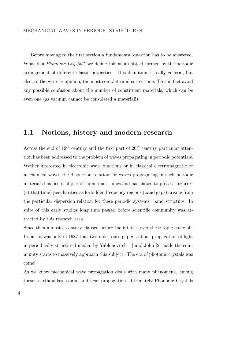
Figure 1.1: Some phenomena where mechanical waves play a fundamental role.
5

1. MECHANICAL WAVES IN PERIODIC STRUCTURES
pass before a consistent number of publications over mechanical counterparts of
photonic crystals (PC exactly) was reached in year 2000 (see Fig. 1.2). However,
as early works on photonic crystals can be dated back to 1888 with the work of
Lord Rayleigh [3], also PC can claim a noticeable ancestor: Leon Brillouin. His
book, titled Wave Propagation in Periodic Structures was published at the end of
Second World War in 1946, and it is curious to tell the story of the copy conserved
here at University’s of Florence library: it was donated from “the american people
trough CARE” as a “response to Unesco reconstruction appeal”. The chance for
Phononic Crystals to have large impact on everyday life was even foreseen by the
just established Unesco!.
Figure 1.2: Growth of publications over Phononic Crystals, the number of
publications is intended per year.
In fact potential applications are wide. They can be realized as waveguides [4] (in
fact a wave, propagating in a homogeneous region sorrounded by a PC, with a char-
acteristic frequency which falls within the band gap of the PC itself, will be guided
6

1.1 Notions, history and modern research
along the path surrounded by the PC), sound barrier [5], delay lines and many
other applicative objects as sound lenses [6] and the legendary acoustic cloak [7].
Moreover the scale invariance which applies to mechanical wave equations (as to
Maxwell’s equation for photonic crystals) allows to extend the operative frequency
range from infrasound [8] (less than 20 Hz) to hypersonic regime [9] (GHz range).
Furthermore PC notion can be applied to different mechanical wave classes as
bulk waves (longitudinal or transverse character), surface waves (Rayleigh or Love
type), or Lamb waves characteristic of plates [10]. Finally periodicity can be real-
ized in one, two or three dimensional fashion.
Figure 1.3: Kinetic sculpture by Eusebio Sempere, built entirely of hollow steel
cylinders arranged in a periodic square array.
The search for periodic elastic composites possessing elastic band gaps was initi-
ated by theoretical works of Kushwaha et al. with two master papers published
in first half of 90s [11], [12]. Major effort in the field has initially concentrated
on elucidating the conditions that favour the formation of band gaps in various
7
1. MECHANICAL WAVES IN PERIODIC STRUCTURES
type of PC (1D, 2D or 3D and solid/solid, or solid/liquid or liquid/liquid), and
the dependance of band gaps width on the filling ratio (substantially, figuring the
PC as a matrix with inclusion, the filling ratio is the ratio between the volume of
inclusions and that of the matrix) [13], [14].
Few years later first experimental studies followed and reached notoriety af-
ter Nature’s publication Sound attenuation by sculpture by R. Martinez-Sala et
al. [15] where attenuation measurements for longitudinal waves lying in the plane
orthogonal to the bars were presented, showing a band gap centered at around 1.7
KHz (see Fig. 1.3). At that time some experimental results were already present,
and others followed. However, before presenting main experimental techniques
trough which PC have been investigated, it is worth to stress that experimental
publications over this topic are really a few when compared to theoretical ones.
Early works [16], [17] can be dated at the very birth of PC research and were real-
ized with Brillouin Light Scatterin (BLS). These report of unexpected behaviour of
the dispersion relation for Rayleigh waves (surface mode, will be back on this in the
next section) in holographic gratings. The BLS technique is particulary suitable
for direct band diagram characterization in fact the exchanged wave vector can be
varied collecting the diffused light at different angles, allowing the band diagram
reconstruction. Finally the technique is particulary appropriate for under micron
PC periodicity, since smaller wave vectors would imply lower frequency Brillouin
peaks that would be hardly resolved due to Rayleigh elastic peak [9], [18].
The most employed experimental technique is that which exploits mechanical
transducers both to excite and reveal waves [19], [20], [21]. In this experiments
sound attenuation measurements are realized. Sometimes they are referred to as
tank-experiments, in that they are worked out in a filled liquid tank were the pe-
riodic solid structures embedded in the liquid realize inclusions. The technique
8

1.1 Notions, history and modern research
can be upgraded employing an imaging system in order to access the displacement
field, recently negative refraction of sound was experimentally demonstrated in
such an experiment [22].
Imaging not exclusively has to be related to a transducer wave source. Depend-
ing on the PC characteristic length it can be associated to optical excitation of
broadband waves [23] (imaging system will obviously differ). In fact it has to be
stressed that nowadays faster mechanical transducers, with the exception of inter-
digital transducers over piezoelectric substrates, reach up to 100 MHz which is any-
how not enough when micrometric or submicrometric structures are investigated.
When considering PC with lattice step at such scale, an all optical investigation
becomes necessary. As already said BLS is suitable for such structures. However
two other experimental technique are available: Picosecond Ultrasonic (PU) and
Transient Grating (TG) experiments. PU is a pump and probe technique [24].
The idea at the basis of this technique is to shine the sample with a short time
optical laser pulse that is absorbed by the material under analysis. This causes
an instantaneous thermal profile in the structure that sets up a stress field which
reveals in propagative waves. The probe laser monitors the induced waves. De-
tection can be realized simply by monitoring the probe intensity variation due to
change in the reflection coefficient (due to the induced strain) or with an interfer-
ometer that detect surface ripples [10]. Many works on PC have been realized with
this technique, e.g. [10], [25], [26], [27]. PU however is not particularly suitable
for band diagram characterization since the pump process generate broad band
wave packet. It is on the contrary TG that shows to be the ad hoc technique
for dispersion relation characterization. Surprisingly when this Ph.D. work was
started one only paper, where PC were studied by means of the TG experiment,
had been published.
Finally it should be remembered that, although the analogies with photonic crys-
9
1. MECHANICAL WAVES IN PERIODIC STRUCTURES
tals are many, the nature of the two types of waves (electromagnetic in the case of
phononic crystals, and elastic in the case of PC) that propagates in the two classes
of metamaterial is completely different. In fact, as it is well known, electromag-
netic waves in isotropic media are pure transverse waves, while elastic waves can
be both transverse and longitudinal. This as many implication when dealing with
the solution of respective governing equations (Maxwell’s equations for the electric
field, mechanical equations for the displacement field): for PC, even in isotropic
materials, the solutions of the equations directly imply the coupling between the
transverse and the longitudinal displacement field so that the polarization state of
the solutions is more complicated than that of the photonic crystals.
At the moment great interest is devoted to the realization of a novel class of
metamaterial that results from the unification of photonic and phononic crystal
properties: phoXonic crystal structures, that would allow a simultaneous control
of the two types of waves [28]. As a matter of fact interaction between photons
and phonons inherently takes place in a large number of optical structures and
devices, and the chance to have control over these phenomena is a just developing
field of research. Great deal of interest, for example, is devoted to the chance
of realizing a, phonon assisted, efficient light emission in silicon. As it is known
silicon present an indirect electronic bandgap so that light emission can take place
only with the exchange of a phonon. The concept is then to realize a periodically
arranged silicon structure to tailor phonons in order to increment the efficiency of
light emission in silicon.
The challenges in front of the PC community are many and still much work has
to be done.
10
1.1 Notions, history and modern research
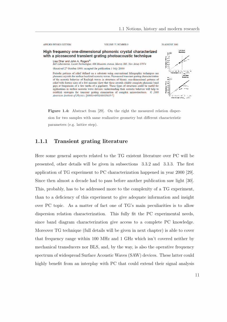
Figure 1.4: Abstract from [29]. On the right the measured relation disper-
sion for two samples with same realizative geometry but different characteristic
parameters (e.g. lattice step).
1.1.1 Transient grating literature
Here some general aspects related to the TG existent literature over PC will be
presented, other details will be given in subsections 3.3.2 and 3.3.3. The first
application of TG experiment to PC characterization happened in year 2000 [29].
Since then almost a decade had to pass before another publication saw light [30].
This, probably, has to be addressed more to the complexity of a TG experiment,
than to a deficiency of this experiment to give adequate information and insight
over PC topic. As a matter of fact one of TG’s main peculiarities is to allow
dispersion relation characterization. This fully fit the PC experimental needs,
since band diagram characterization give access to a complete PC knowledge.
Moreover TG technique (full details will be given in next chapter) is able to cover
that frequency range within 100 MHz and 1 GHz which isn’t covered neither by
mechanical transducers nor BLS, and, by the way, is also the operative frequency
spectrum of widespread Surface Acoustic Waves (SAW) devices. These latter could
highly benefit from an interplay with PC that could extend their signal analysis
11
1. MECHANICAL WAVES IN PERIODIC STRUCTURES
capability .
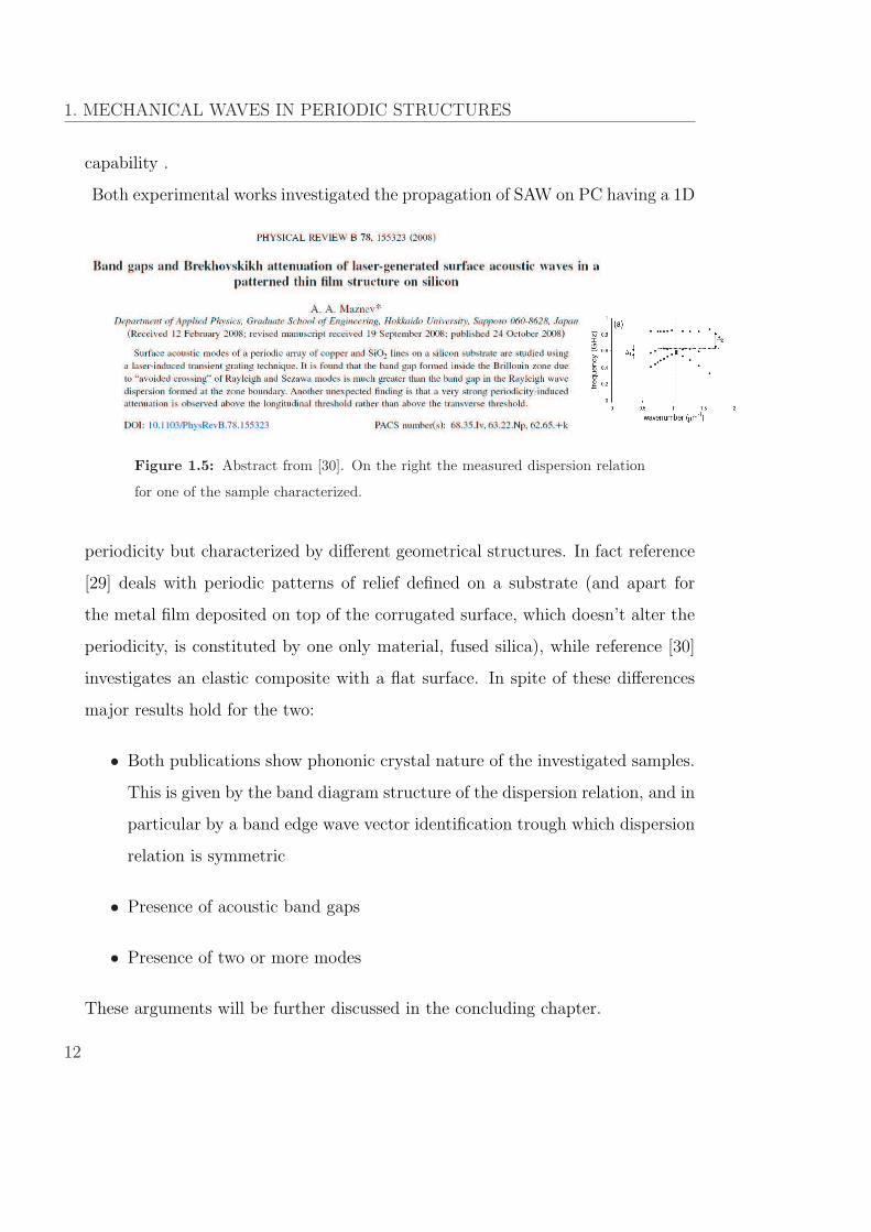
Both experimental works investigated the propagation of SAW on PC having a 1D
Figure 1.5: Abstract from [30]. On the right the measured dispersion relation
for one of the sample characterized.
periodicity but characterized by different geometrical structures. In fact reference
[29] deals with periodic patterns of relief defined on a substrate (and apart for
the metal film deposited on top of the corrugated surface, which doesn’t alter the
periodicity, is constituted by one only material, fused silica), while reference [30]
investigates an elastic composite with a flat surface. In spite of these differences
major results hold for the two:
• Both publications show phononic crystal nature of the investigated samples.
This is given by the band diagram structure of the dispersion relation, and in
particular by a band edge wave vector identification trough which dispersion
relation is symmetric
• Presence of acoustic band gaps
• Presence of two or more modes
These arguments will be further discussed in the concluding chapter.
12

1.2 Theoretical elements
1.2 Theoretical elements
This section is organized in three subsections. The first one is devoted to the
introduction of the dynamic equations for an inhomogeneous elastic body. The
second will recall some general arguments about the propagation of surface acoustic
waves. The third will recall the keynotes of periodic systems: general arguments
over direct and reciprocal lattice, and the wave equation in periodic media.
1.2.1 Linear elasticity elements
Along this section mechanics of solid bodies, regarded as continuous media will be
presented. References [31] and [12] are the guidelines that have been adopted here
to develop the theory of elasticity, we have heavily exploited them due to their
clearness.
Under the action of applied forces, solid bodies exhibit deformation, i.e. they
change in shape and volume. Deformations can be defined rigorously in the fol-
lowing way. The position of any point in in the body is defined by its radius vector
r (with components x1 = x, x2 = y, x3 = z) in some coordinate system. When the
body is deformed, every point in it is in general displaced. Let us consider some
particular point; let its radius before deformation be r, and that after deformation
be r′(with components x
′i). The displacement of this point due to the deformation
is then given by the vector r - r′which we shall denote by u:
ui = x′i − xi (1.1)
The vector u is called the displacement vector. The coordinates x′i of the displaced
point depend obviously on the coordinate xi of the point . Therefore if the vector
u is given as a function of xi, the deformation of the body is entirely determined.
When a body is deformed, the distances between its points change. Let us consider
two points very close one to another. If the radius vector joining them before
13

1. MECHANICAL WAVES IN PERIODIC STRUCTURES
deformation is dxi, the radius vector joining the same two points when the body
is deformed is dx′i = dxi + dui. The distance between the points before and after
the deformation will be dl =√
dx21 + dx2
2 + dx23, and dl
′=
√dx
′12 + dx
′22 + dx
′32
respectively. Using the rule of summation over repeated indices we can write
dl2 =∑
i=1 3dx2i , dl
′2 =∑
i=1 3dx′i2 =
∑i=1 3(dxi + dui)
2. Substituting dui =
(∂ui/∂xk)dxk we get
dl′2 = dl2 + 2
∂ui
∂xk
dxidxk +∂ui
∂xk
∂ui
∂xl
dxkdxl (1.2)
Since the summation is taken over both suffixes i and k in the second term, on the
right hand side of the equation we can put (∂ui/∂xk)dxidxk = (∂uk/∂xi)dxidxk.
In the third term, we interchange the suffixes i and l. Then dl′2 takes the form
dl′2 = dl2 + 2uikdxidxk (1.3)
where the tensor uik is defined as
uik =1
2(∂ui
∂xk
+∂uk
∂xi
+∂ul
∂xi
∂ul
∂xk
) (1.4)
' 1
2(∂ui
∂xk
+∂uk
∂xi
) (1.5)
The tensor uik is called strain tensor and is, by definition,symmetrical. The third
term of the summation in the right hand side of eq. (1.4) can be dropped down
when small deformations are considered , i.e. linear elasticity approximation is
considered (eq. (1.5)). We will assume that this approximation applies to the in-
vestigated samples.
In a body that is not deformed, the arrangement of molecules corresponds to a
state of thermal equilibrium, then all parts of the body are in mechanical equilib-
rium.
When a deformation occurs molecule’s arrengment is changed, and the body ceases
to be at rest. Therefore the body returns to the original equilbrium state by means
14

1.2 Theoretical elements
of forces that arises due to the deformation itself. This internal forces are known
as internal stresses, and in the following we will consider that internal stresses
are only governed by elastic forces (Hooke’s law) without any contribution from
eventual stresses arising from pyroelectric or piezoelectric effects.
We can now write down the equations of dynamics. We consider an inhomo-
geneous, however isotropic and linearly elastic solid of infinite extension. At every
point r the medium is characterized by three purely mechanical parameters: the
mass density ρ(r), the longitudinal speed of sound cl(r) and the transverse speed
of sound ct(r). In terms of these the stress tensor assumes the form
σij = 2ρc2t uij + ρ(c2
l − c2t )ullδij (1.6)
where the summation over repeated indices (throughout all the text) convention
is adopted, then Newton’s law of dynamic reads [12]
ρ∂2ui
∂t2=
∂σij
∂xj
(1.7)
= ρc2t∇2ui + ρ(c2
l − c2t )
∂
∂xi
∇ · u +∇(ρc2t ) · ∇ui (1.8)
+∇(ρc2t ) ·
∂u
∂xi
+ [∂
∂xi
(ρc2l − 2ρc2
t )]∇ · u (1.9)
after some algebra this can be brought into the form
ρ∂2ui
∂t2= ∇ · (ρc2
t∇ui) +∇ · (ρc2t
∂
∂xi
u) +∂
∂xi
[(ρc2l − 2ρc2
t )∇ · u] (1.10)
Equation (1.10) represents the elastic wave equation for an inhomogeneous elas-
tic medium. It is somehow complicated, with respect to that of an homogeneous
medium, since with ρ, cl and ct being position dependent the equation cannot be
separated into two independent equations, one for the longitudinal displacement
(that satisfies ∇ × u = 0) and the other for the transverse displacement (with
∇ · u = 0).
15

1. MECHANICAL WAVES IN PERIODIC STRUCTURES
1.2.2 Surface Acoustic Waves
Here some general notions about waves propagating at the free surface of a body
will be considered. The approach to the surface waves theory presented here is
not intended to be neither complete, nor detailed or analytical, but, instead, will
only focus on general aspects of main interest to this Ph.D. thesis: qualitative key
points on some specific types of surface waves will be presented here.
Let us consider the case of a homogeneous, isotropic finite media. Bulk waves will
continue to be a solution of the equations (1.10) but other solution are present at
the boundaries of the body (on the surface).
Let us consider the sagittal plane (in red in Fig. 1.6), that is the plane containing
both the normal to the surface and the wave vector (lying in the surface), it can be
shown that surface waves contained in this plane are decoupled from those in the
plane orthogonal to the sagittal one. Surfaces acoustic waves (SAW) contained in
the sagittal plane are semi-transverse (longitudinal and transverse displacements
aren’t decoupled). They’re usually referred to as Rayleigh waves. SAW lying in
the plane orthogonal to the sagittal plane will have a pure transverse character
and are known as Love waves. In the rest of this thesis only Rayleigh SAW will
be considered (sometime only the acronym SAW will be used).
The equation of motion predicts, in the case of an homogeneous body, a single SAW
mode (the Rayleigh mode) which is non dispersive (upper right part in Fig. 1.6).
The sound speed cR have an empirical expression given by the Viktorov formula
cR ' 0.87 + 1.12ν
1 + νct (1.11)
where ν is the Poisson’s ratio. Obviously cR < ct.
The Rayleigh is a guided mode, the associated displacement field decays exponen-
tially with depth in the material. At a depth of some wavelengths, no displacement
is associated to the wave propagating at the surface.
16

1.2 Theoretical elements
Semi-infinite media
Semi-infinite media + film
Figure 1.6: In red the sagittal plane. Two different cases are that of a free
homogeneous surface of a semi-infinite media or that of a film bounded to the
surface. Different dispersion relation are related to the two cases.
In order to perform our experimental investigation of SAW we are forced to use
samples characterized by an high reflection coefficient. This is achieved realizing
a thin metal film on the sample surface. The equation of motion of the system is
then modified and hence the SAW definition [32].
When a film is bounded to the surface several modes can be guided along the
surface (lower right part in Fig. 1.6). Two general cases can be distinguished:
“fast” films over “slow” substrates, and viceversa. We will focus on the latter case
17

1. MECHANICAL WAVES IN PERIODIC STRUCTURES
Figure 1.7: Dispersive character of the modes guided along the surface of a
body constituted by a “fast” substrate and a “slow” film. In this graph the phase
velocity is plotted against the product of the wavector associated to the wave and
the film thickness [32]. To interprete the meaning of the indicated values please
note that: V stands for velocity, the subscript t (R, lg) for transverse (Rayleigh
or longitudinal respectively), while subscript s (f) is indicating a substrate (or
film) property.
(“slow” films over “fast” substrates) as the samples studied along this Ph.D. work
fit this class. As it has been said many dispersive modes can be supported. To
clarify the behaviour of these surface waves (generally first order mode is named
Rayleigh mode and higher orders are called Rayleigh-Sezawa modes or simply
higher order Rayleigh modes) the Fig. 1.7 taken from [32] results useful. Here the
phase velocity of the wave is plotted against the product of the wave vector (k)
associated to the wave itself and the film thickness (h).
As it can be seen depending on the kh value more modes can be supported by the
surface. For high values of kh (a film thickness much bigger than the wavelength
18
1.2 Theoretical elements
of the wave itself) the displacement will mainly involve the film itself and its
properties will be sensed. In fact, as shown in Fig. 1.7, the Rayleigh mode will
have a velocity that at limit approaches the Rayleigh velocity of the film while
Rayleigh-Sezawa modes will tend to the film’s transverse velocity.
For low values of the product kh (that means waves characterized by a wavelength
much bigger than the film thickness) the first mode approaches the value of the
Rayleigh mode of the substrate. Higher order mode have a phase velocity cutoff
(we’ll be back on the meaning of this cutoff in last chapter) given by the transverse
velocity of the substrate itself. In some way when the wavelength is much bigger
than the film thickness the wave senses only a little the presence of the film as
the wave’s associated displacement involves (penetrating in depth for about a
wavelength) mainly the substrate.
In the experimental investigation reported in this work the product kh < 0.14 so
that the substrate properties can be easily investigated.
1.2.3 Periodic systems and lattices
As this thesis deals mainly with waves propagating in spatially periodic structures,
here we want to recall the basic properties and definition over such structures.
The starting point in the description of the symmetry of any periodic arrangement
is the concept of Bravais lattice. The Bravais Lattice is defined as an infinite
spatial array of discrete points with such an arrangement and orientation that it
appears exactly the same from whichever of its points the array is viewed [33].
Mathematically, a three dimensional Bravais lattice is defined as a collection of
point with position vectors R of the form
R =3∑
i=1
miai (1.12)
19
1. MECHANICAL WAVES IN PERIODIC STRUCTURES
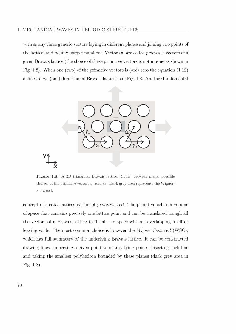
with ai any three generic vectors laying in different planes and joining two points of
the lattice; and mi any integer numbers. Vectors ai are called primitive vectors of a
given Bravais lattice (the choice of these primitive vectors is not unique as shown in
Fig. 1.8). When one (two) of the primitive vectors is (are) zero the equation (1.12)
defines a two (one) dimensional Bravais lattice as in Fig. 1.8. Another fundamental
a1a1
a2a2
Figure 1.8: A 2D triangular Bravais lattice. Some, between many, possible
choices of the primitive vectors a1 and a2. Dark grey area represents the Wigner-
Seitz cell.
concept of spatial lattices is that of primitive cell. The primitive cell is a volume
of space that contains precisely one lattice point and can be translated trough all
the vectors of a Bravais lattice to fill all the space without overlapping itself or
leaving voids. The most common choice is however the Wigner-Seitz cell (WSC),
which has full symmetry of the underlying Bravais lattice. It can be constructed
drawing lines connecting a given point to nearby lying points, bisecting each line
and taking the smallest polyhedron bounded by these planes (dark grey area in
Fig. 1.8).
20

1.2 Theoretical elements
b1
b2
Figure 1.9: The reciprocal lattice of the 2D triangular Bravais lattice shown
in Fig. 1.8 is (arbitrary) represented with green crosses. It is a triangular lattice
as the direct one. The reciprocal lattice is rotated of 30◦ with respect to direct
lattice. The same applies to the WSC. In red the basis resulting from the the
direct basis choice a1 and a2 shown on the right of Fig. 1.8. Green arrows indicate
that the lattice has infinite extent.
The Bravais lattice, which is defined in real space, is sometimes referred to as
direct lattice. At the same time there exists the concept of reciprocal lattice, which
play a fundamental role in virtually any study of any wave phenomena in periodic
structures. For any Bravais lattice R in real space given by equation (1.12) there
exist a set of wavectors G, that constitute the reciprocal lattice in the reciprocal
space (the space of wave vectors), satisfying
e[i·(G·R)] = 1 (1.13)
for every R in the direct lattice. The reciprocal lattice is a Bravais lattice itself.
21

1. MECHANICAL WAVES IN PERIODIC STRUCTURES
The primitive vectors bi of the reciprocal lattice are constructed from the primitive
vectors ai of the direct lattice by the following expressions
b1 = 2πa2 ∧ a3
a1 · (a2 ∧ a3)
b2 = 2πa3 ∧ a1
a2 · (a3 ∧ a1)(1.14)
b3 = 2πa1 ∧ a2
a3 · (a1 ∧ a2)
As the reciprocal lattice is a Bravais lattice one can identify its WSC, conven-
tionally called first Brillouin zone (contained within the red hexagon in Fig. 1.9).
Of particular interest is the irreducible Brillouin zone (ZIB) (red area in Fig. 1.9)
along whose boundaries the properties of the periodic medium under analysis can
be fully characterized.
The equation (1.10) is valid for an arbitrary inhomogeneity. Now we focus
on inhomogeneous material which exhibits spatial periodicity. This implies that
all the material properties ρ(r), cl(r) and ct(r) may be expanded in Fourier series.
Actually it is convenient to expand ρc2l and ρc2
t rather than cl and ct themselves [12]
ρ(r) =∑G
ρ(G)eiG·r
ρ(r)c2l (r) =
∑G
Λ(G)eiG·r (1.15)
ρ(r)c2t (r) =
∑G
τ(G)eiG·r
The periodicity of the medium may be three, two or one dimensional, the reciprocal
lattice vector has corresponding dimensionality. The summation in (1.15) extends
over the infinite reciprocal lattice that correspond to the Bravais lattice in real
space. The displacement, associated to the generic wave vector k, uk(r) must
22

1.2 Theoretical elements
satisfy the Bloch theorem
uk(r) = ei(k·r−ωt)∑G
uk(G)eiG·r (1.16)
where ω is the circular frequency of the wave. Substitution of equations (1.16)
and (1.15) in equation (1.10), and the use of some vector algebra together with
the multiplication by exp(−iG′′ · r) and integration over the unit cell, gives the
result
∑
G′{τ(G−G′)uk(G
′)(k+G′)·(k+G)+τ(G−G′)uk(G′)·(k+G)(k+G′)+ (1.17)
+[Λ(G−G′)− 2τ(G−G′)]uk(G′) · (k + G′)(k + G)− ω2ρ(G−G′) = 0
If we allow G to take all the points of the reciprocal lattice, then equation (1.17)
is an infinite set of linear equations for the eigenvectors uk(G). For a given value
of the wave vector k this set of equations has solution for some eigenvalues ωn(k),
where n = 1, 2, ... is the first, second, etc. vibrational band. Then if we plot
the eigenvalues ωn obtained for the values of the Bloch wave vector k along the
ZIB we obtain the so-called band diagram, which is nothing else than the relation
dispersion characteristic of the periodic system under study.
23


Chapter 2SAMPLES AND EXPERIMENTAL
TECHNIQUE
This chapter is composed of two main sections. In the first one a detailed pre-
sentation of the experimental technique adopted to investigate the sample and a
theoretical analysis of the measured signal will be given. In the second section the
investigated samples will be presented.
2.1 Transient Grating experiment
The Transient Grating experiment (TG) is a time resolved optical technique, based
on non linear optical effects [34], it is indeed a particular case of the large category
of the so called four-wave-mixing techniques [35, 36]. This experimental tool is
particularly suitable to measure mechanical, acoustic, viscous and thermal phe-
nomena in solids as in liquids. It enables the investigation of a very wide temporal
range, from nanosecond to millisecond. Thanks to the Heterodyne Detection (HD)
(a detailed description will follow) the measured signal is characterized by an ex-
cellent signal to noise ratio. Definitely, HD-TG experiments can be considered an
25
2. SAMPLES AND EXPERIMENTAL TECHNIQUE
important breakthrough within the framework of the optical techniques, because
of their capability to measure many different dynamics in a time window where
alternative methods fail.
It has to be stressed that two possible configurations of the experiment are possible:
• Transmission geometry: suitable to investigate bulk properties of semi-transparent
materials.
• Reflection geometry: suitable to investigate superficial properties of reflect-
ing media.
As already pointed out during this Ph.D. work all measurement have been realized
in this latter configuration.
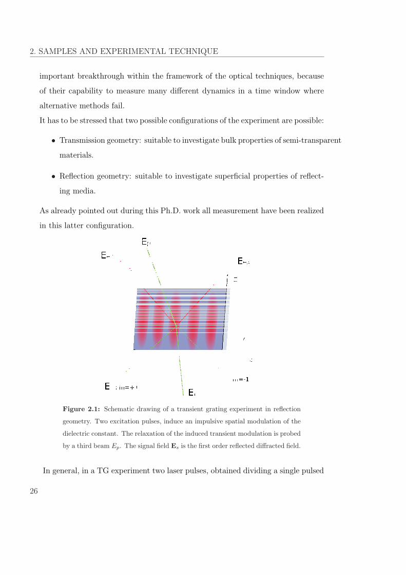
Figure 2.1: Schematic drawing of a transient grating experiment in reflection
geometry. Two excitation pulses, induce an impulsive spatial modulation of the
dielectric constant. The relaxation of the induced transient modulation is probed
by a third beam Ep. The signal field Es is the first order reflected diffracted field.
In general, in a TG experiment two laser pulses, obtained dividing a single pulsed
26

2.1 Transient Grating experiment
laser beam, are made to interfere on a sample (over its surface or in bulk depending
on the mechanical waves under study) and generate a spatially periodic variation
of the optical material properties (e.g. refractive index) due to radiation-matter
interaction phenomena. [36–38].This modulation is probed by a third laser beam,
typically of different wavelength from that of the pump; it can be either a pulsed
or a continuous-wave (CW) beam. It impinges on the induced grating and it is
subsequently diffracted by it (be it reflected or transmitted). The diffracted signal
provides information on the relaxing grating, then on the induced dynamics.
p
ex
1E
ex
2E
Ep
qex
s
Es
x
y
k1
k2
Figure 2.2: Schematic drawing of a transient grating experiment in transmis-
sion geometry. Two excitation pulses, Eex1 and Eex
2 induce an impulsive spatial
modulation of the dielectric constant with step Λ. The relaxation of the induced
transient modulation is probed by a third beam, Ep.
Schematic drawings of a TG experiment are shown in Fig. 2.1 and Fig.2.2. To
be as clear as possible the details are shown in the transmission geometry figure,
however the same holds for the reflection geometry. The spatial modulation is
characterized by the wave-vector q, equal to the wave-vector difference (k1 − k2)
of the two pump pulses. Its modulus is:
q =4π sin (θex)
λex
, (2.1)
27
2. SAMPLES AND EXPERIMENTAL TECHNIQUE
where λex and θex are the wavelength and the incidence angle of the exciting pulses,
respectively.
2.1.1 Signal definition
Concentrating over excitation of surface acoustic waves in metals we consider that
radiation-matter interaction between pump light and metallic surface is dominated
by absorption phenomena due to free electrons. In fact the free electrons rapidly
absorb pump light and instantaneously (relatively to the experimental temporal
resolution, that corresponds to few tens of picoseconds) relax via non-radiative
channels generating a local heating. So that, soon after pump light absorption,
the interference optical grating rapidly turns into a temperature grating. The
rapid conversion of electromagnetic energy into heat enables to separate the pump
process from the probing.
The probe process consists in detecting the first order reflected diffracted field Es
(shown in Fig. 2.1) of the probe field Ep (wave vector kp). To what the wave
vector ks of Es is involved, normal reflection rules apply to the y and z component
(ks y = −kp y, ks z = kp z), while the x component of the diffracted field is related
to the diffraction from the induced grating
ks x = kp x + q. (2.2)
In order to define the measured signal it is useful to introduce the ratio between
the amplitude of the i-th component (the 1,2,3 indices stand for x,y,z axis) of the
probe field Ep i and that of the electromagnetic field E′p i, given by the interaction
of the probe beam with the metallic surface eventually modified from the gratings
generated by the pump light absorption (we will illustrate these phenomena in the
28
2.1 Transient Grating experiment
following), in the very surface proximity
E′p i(x, y, z = ε, t) = RijEp j (2.3)
The E′p i distribution generates, in the far field condition the reflected field and the
diffracted beams. The ij element of the complex reflection tensor R is defined as
the product of an amplitude and a phase term
Rij = rijei·ϕij (2.4)
In what way a grating induced on the surface affects this field? The pump in-
duced grating results as a thin, sinusoidal amplitude and phase grating along the
surface (which is, moreover, no longer flat but sinusoidally rippled due to thermal
expansion, with a ripple amplitude ε around the flat value z=0. This turns to
be an extra phase-grating contribution that, only for the moment, we neglect).
Since modulations of the pump induced gratings are weak the two effects can be
considered, in first approximation, as independent.
The amplitude modulation produce a field distribution at the very surface prox-
imity
E′p i = [rij + ∆rij(t) cos(qx)]ei·ϕijEp j (2.5)
where ∆rij(t) cos(qx) is the amplitude variation of the ij element of the reflection
tensor induced by the amplitude transient grating. The reflected electromagnetic
field and the diffracted orders fields in the far-field approximation (distance y
from the surface satisfies y >> Λ2/λ, with λ electromagnetic wavelength) can be
obtained within the framework of Fourier optics and is proportional to the Fourier
transform of the electromagnetic field distribution at the surface [39]. It can be
shown that the first order reflected diffracted field (Es) distribution is then
Es i ∝ ∆rij(t, q)Ep j (2.6)
29

2. SAMPLES AND EXPERIMENTAL TECHNIQUE
Similarly the phase modulation generated by the grating induces a field distribu-
tion
E′p i = rije
i·[ϕij+∆ϕij(t) cos(qx)]Ep j (2.7)
where ∆ϕij(t) cos(qx) is the phase variation in the ij element of the reflection
tensor induced by the transient phase grating. In this case, it can be shown that
the first order reflected diffracted field distribution is
Es i ∝ i∆ϕij(t, q)Ep j (2.8)
When a phase grating and an amplitude grating are present at the same time and
weak grating approximation is considered (induced variations are few percentage of
the unperturbed reflection coefficients), the previous results still hold for the sum
of the two contributions: first order diffracted reflected field is simply proportional
to the sum of the induced variations
Es i ∝ [∆rij(t, q) + i∆ϕij(t, q)]Ep j (2.9)
The reflectivity tensor is defined by the dielectric tensor εij and so to the
experimental observables. In a metal the dielectric tensor is complex
εij = ε′ij + iε
′′ij (2.10)
It can be shown that [40] transient grating induced variations ∆rij and ∆ϕij can be
written in terms of transient grating induced variations of the real and imaginary
components of dielectric tensor as
∆rij = a∆ε′ij + b∆ε
′′ij (2.11)
∆ϕij = c∆ε′ij + d∆ε
′′ij (2.12)
where the constants a, b, c, and d are parameters proper of the metal considered.
In conclusion the real and imaginary part of the dielectric variation tensor can be
30
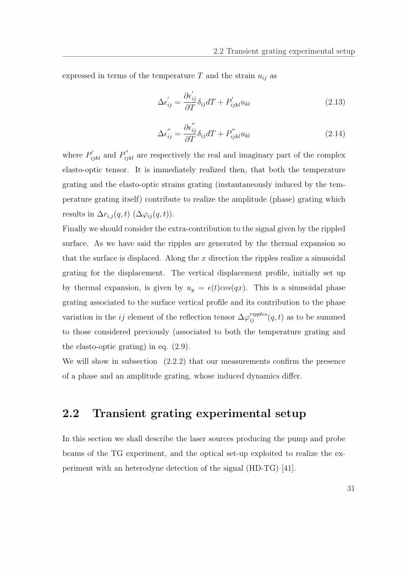
2.2 Transient grating experimental setup
expressed in terms of the temperature T and the strain uij as
∆ε′ij =
∂ε′ij
∂TδijdT + P
′ijklukl (2.13)
∆ε′′ij =
∂ε′′ij
∂TδijdT + P
′′ijklukl (2.14)
where P′ijkl and P
′′ijkl are respectively the real and imaginary part of the complex
elasto-optic tensor. It is immediately realized then, that both the temperature
grating and the elasto-optic strains grating (instantaneously induced by the tem-
perature grating itself) contribute to realize the amplitude (phase) grating which
results in ∆ri,j(q, t) (∆ϕij(q, t)).
Finally we should consider the extra-contribution to the signal given by the rippled
surface. As we have said the ripples are generated by the thermal expansion so
that the surface is displaced. Along the x direction the ripples realize a sinusoidal
grating for the displacement. The vertical displacement profile, initially set up
by thermal expansion, is given by uy = ε(t)cos(qx). This is a sinusoidal phase
grating associated to the surface vertical profile and its contribution to the phase
variation in the ij element of the reflection tensor ∆ϕripplesij (q, t) as to be summed
to those considered previously (associated to both the temperature grating and
the elasto-optic grating) in eq. (2.9).
We will show in subsection (2.2.2) that our measurements confirm the presence
of a phase and an amplitude grating, whose induced dynamics differ.
2.2 Transient grating experimental setup
In this section we shall describe the laser sources producing the pump and probe
beams of the TG experiment, and the optical set-up exploited to realize the ex-
periment with an heterodyne detection of the signal (HD-TG) [41].
31
2. SAMPLES AND EXPERIMENTAL TECHNIQUE
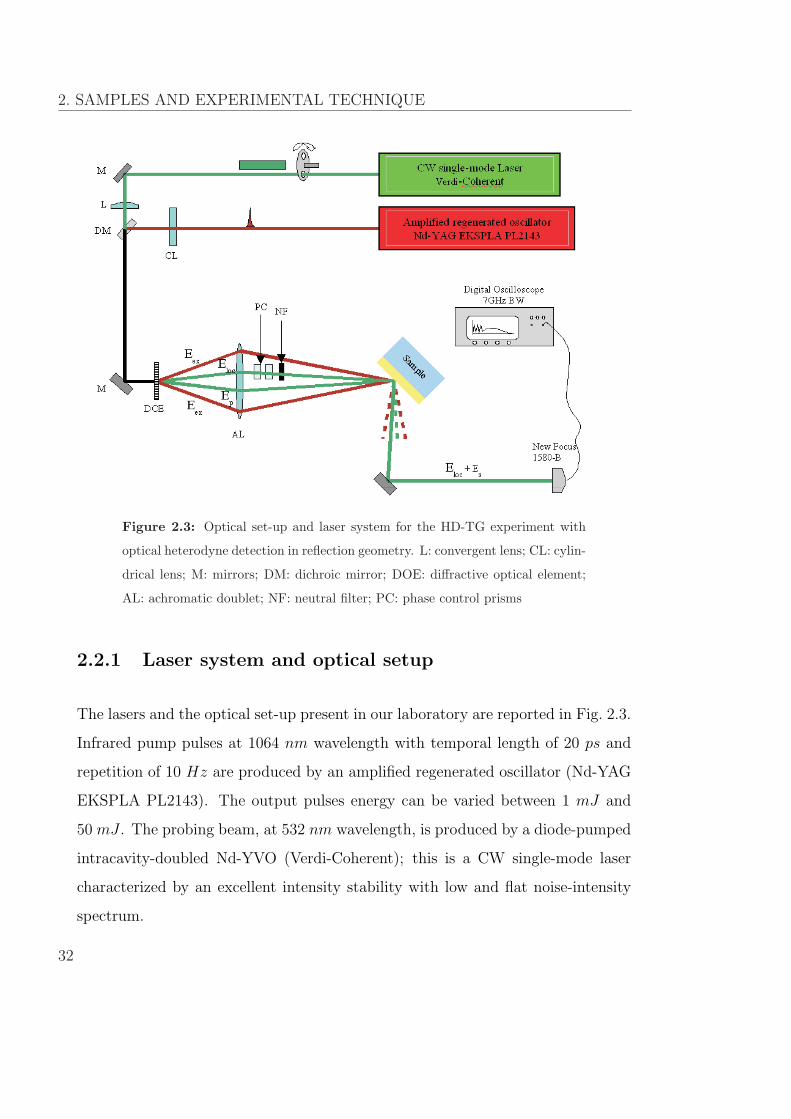
Figure 2.3: Optical set-up and laser system for the HD-TG experiment with
optical heterodyne detection in reflection geometry. L: convergent lens; CL: cylin-
drical lens; M: mirrors; DM: dichroic mirror; DOE: diffractive optical element;
AL: achromatic doublet; NF: neutral filter; PC: phase control prisms
2.2.1 Laser system and optical setup
The lasers and the optical set-up present in our laboratory are reported in Fig. 2.3.
Infrared pump pulses at 1064 nm wavelength with temporal length of 20 ps and
repetition of 10 Hz are produced by an amplified regenerated oscillator (Nd-YAG
EKSPLA PL2143). The output pulses energy can be varied between 1 mJ and
50 mJ . The probing beam, at 532 nm wavelength, is produced by a diode-pumped
intracavity-doubled Nd-YVO (Verdi-Coherent); this is a CW single-mode laser
characterized by an excellent intensity stability with low and flat noise-intensity
spectrum.
32

2.2 Transient grating experimental setup
The two beams are collinearly coupled by the dichroic mirror DM and sent on
the grating phase (DOE Diffractive Optical Element), described in detail later.
This produces the two excitation pulses, Eex, the probing, Ep, and the reference
beam, El. These beams, cleaned by a spatial mask of other diffracted orders,
are collected and focused on the sample’s surface by an achromatic doublet (AL,
f = 160 mm). This optical element is mounted over a slide guide to translate
along the optical axis in order to vary the magnification of the system and so the
induced wave vector. In this way the excitation grating produced on the sample is
an image of the enlightened DOE phase pattern whose magnification is established
by the AL position [42], [43]. The local laser field is also attenuated by a neutral
density filter NF and adjusted in phase by with the use of a pair of quartz prisms
that allow to vary the optical path of El with respect to Ep, and so their relative
phase (to avoid confusion please note that in Fig. 2.3, PC stand for Phase Control).
The HD-TG signal is optically filtered from eventual spurious components and
measured by a fast photodiode, New Focus model 1580-B with a bandwidth of
DC−12 GHz. The signal is then recorded by a digital oscilloscope with a 7 GHz
bandwidth (at the voltage scale we work it reduces down to about 1 GHz) and
a 20 Gs/s sampling rate (Tektronix). The measured signals have a typical tem-
poral duration of some microseconds so the time window of the oscilloscope. The
sampling of the signal is the maximum allowed by the oscilloscope: 50 ps time-
step). Each scan is an average of 1000 recordings, which is sufficient to produce
an excellent signal to noise ratio.
We reduced the laser energy on the samples to the lowest possible level to
avoid undesirable thermal effects, and the CW beam has been gated in a window
of about 3 ms every 100 ms by using a mechanical chopper synchronized with the
excitation pulses. Depending on the induced wave vector, the mean exciting energy
was in the range 0.4−4 mJ for each pump pulse and the probing power was about
33
2. SAMPLES AND EXPERIMENTAL TECHNIQUE
10− 100 mW. The reference beam intensity is very low; it was experimentally set
by means of a variable neutral filter in order to be almost 100 times the intensity
of the diffracted signal. With these intensities, the experiment was well inside the
linear response regime and no dependence of HD-TG signal shape on the intensities
of the beams could be detected.
As already stated in the introduction, the diffractive optical element DOE was
first introduced in 1998 [42,43]. It provides considerable advantages. It is a trans-
mission phase grating, characterized by a square shaped profile, is hollowed out
on a fused silica plate by ion beam techniques. Thanks to the square profile of
the grating, it is possible to obtain very high diffraction efficiency on the only
first orders by controlling the depth ∆ of the grooves. Choosing ∆ = λ/2(n−1)
, with
n the refractive index of silica, the diffraction efficiency would be, theoretically,
maximized on each first order. Since we have to diffract both 1064 and 532 nm
beams, a compromise must be reached. The chosen DOE is optimized for 830 nm
radiation, and it gives on a single beam at first order a 12% diffraction efficiency
for the 532 nm and 38% for the 1064 nm.
Some important features have to be emphasized. With this set-up automatic
collimation of local field and diffracted field is obtained with the further advan-
tage of a very stable phase locking between the probing and reference beam: two
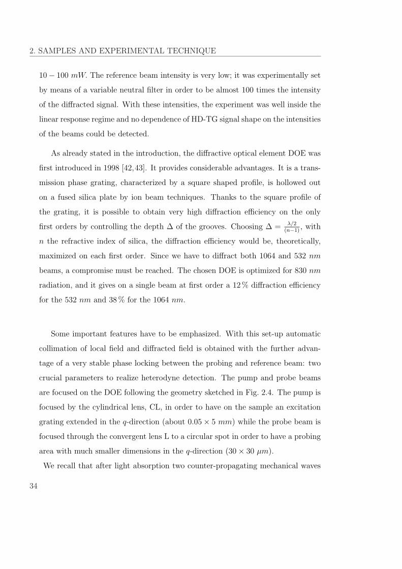
crucial parameters to realize heterodyne detection. The pump and probe beams
are focused on the DOE following the geometry sketched in Fig. 2.4. The pump is
focused by the cylindrical lens, CL, in order to have on the sample an excitation
grating extended in the q-direction (about 0.05× 5 mm) while the probe beam is
focused through the convergent lens L to a circular spot in order to have a probing
area with much smaller dimensions in the q-direction (30× 30 µm).
We recall that after light absorption two counter-propagating mechanical waves
34
2.2 Transient grating experimental setup
Figure 2.4: Drawing of the cylindrical spot shape of pump and the circular spot
of probe on the DOE.
are launched in the q-direction and their superposition gives rise to a stationary
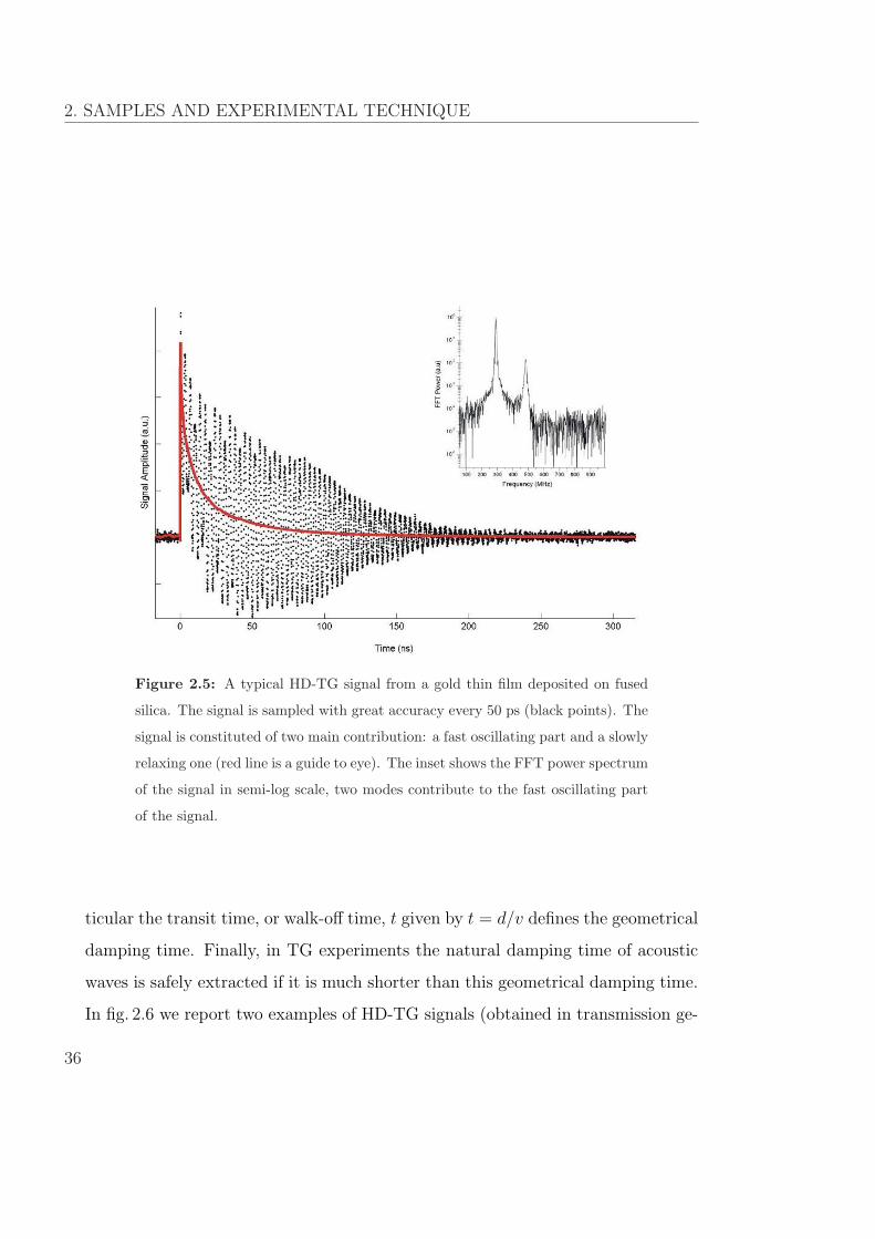
wave. As it can be seen in Fig. 2.5 the experimental data are composed by a
fast oscillating contribution (mechanical waves contribution) and a slowly relaxing
term (thermal relaxation). Fourier transform of the signal allows to extract the
frequency content of the excited mechanical waves in correspondence of the peaks
(shown in the inset of Fig. 2.5): two different mode are excited, first is at about
280 MHz, the second at 470 MHz. Fourier transform is realized with a Fast
Fourier Transform (FFT) routine. Comments over the nature of these modes are
postponed to the last chapter.
What about the damping of the sound? Clearly, the two induced waves have a
spatial extension in the q-direction which is limited by the dimension of the in-
duced grating that is clearly related to the dimension of the pump pulses. Thus,
the induced stationary wave has a life time due to geometrical features. This geo-
metrical time depends on the pump spatial extension 2d in the q-direction and on
velocity v at which the counterpropagating waves travel , i.e. on the sound phase
velocity (group velocity in dispersive media) of the investigated material. In par-
35
2. SAMPLES AND EXPERIMENTAL TECHNIQUE
Figure 2.5: A typical HD-TG signal from a gold thin film deposited on fused
silica. The signal is sampled with great accuracy every 50 ps (black points). The
signal is constituted of two main contribution: a fast oscillating part and a slowly
relaxing one (red line is a guide to eye). The inset shows the FFT power spectrum
of the signal in semi-log scale, two modes contribute to the fast oscillating part
of the signal.
ticular the transit time, or walk-off time, t given by t = d/v defines the geometrical
damping time. Finally, in TG experiments the natural damping time of acoustic
waves is safely extracted if it is much shorter than this geometrical damping time.
In fig. 2.6 we report two examples of HD-TG signals (obtained in transmission ge-
36

2.2 Transient grating experimental setup
0.0 0.1 0.2 0.3 0.4 0.5
HD
-TG
sign
al (a
rb. u
n.)
Time ( s)
Figure 2.6: Comparison between HD-TG transmission geometry signal on fused
silica (upper graph) and CCl4 (lower graph). In the first case, the damping is
dominated by the gaussian spatial shape of the pumps, whereas in the second we
probe exclusively the natural damping.
ometry) where the geometrical damping and natural damping differently affect the
respective signal. In the upper graph the HD-TG signal obtained for fused silica,
whose natural damping time is very long compared the the geometrical: here the
acoustic oscillations decay with a gaussian profile due to the pump gaussian shape.
In the loweer graph, instead, we show the HD-TG signal obtained in CCl4: here
the pump width is extended enough to measure the exponential natural damping
which is much shorter that in silica one. In the silica case we can observe also an
other phenomenon. At around 400 ns the oscillations suddenly death. In this case
the cylindrical focalization has a dimension larger than the 5 mm width of the
phase mask. This dimension, considering the silica sound velocity of 6000 m/s,
fixes the maximum measurable time window for the acoustic oscillation which is
37

2. SAMPLES AND EXPERIMENTAL TECHNIQUE
around 400 nm.
2.2.2 Heterodyne and Homodyne detections
Typically, detectors of electromagnetic field measure the intensity:
S (t) = Is (t) =⟨|E(t)|2⟩
op.c., (2.15)
where 〈·〉op.c. means the time averaging over the optical period1. A direct measure-
ment of the scattering intensity is called homodyne detection (HO). If the measured
field is a signal field supplying dynamic information about some relaxing system,
like in a TG experiment, through a response function R (t) (i.e. Es (t) ∝ R (t)),
the homodyne signal is clearly proportional to the square of the response function.
Another detection mode exists by which it is possible to directly measure the
amplitude of the diffracted field; this detection mode is called optical heterodyne
detection (HD). In HD, both the signal (the first order reflected diffracted field) and
reference field are superimposed on the detector, and the intensity of interference
field is recorded. In general Es can be written as
Es(t) = eEs (t) exp [i (ks · r− ωt)] + c.c., (2.16)
with Es(t), in general, a complex function; then we choose a reference field with
same wave-vector, direction and frequency of Es(t) and with constant amplitude
El(t) = eEl exp [i (ks · r− ωt + φ)] + c.c., where φ is the optical phase between the
signal and reference field and El is a real amplitude. Hence, the heterodyne signal
is
S (t) =⟨|Es(t) + El|2
⟩op.c.
(2.17)
= Is(t) + Il + 2{Re[Es(t)]El cos φ + Im[Es(t)]El sin φ}.1Strictly speaking the average will be performed over the detector integration time, which
even in ultrafast detectors is much longer than the time of optical cycle but generally shorter
than the signal relaxation times.
38

2.2 Transient grating experimental setup
The first two terms in the right-hand side of eq. 2.17 are the homodyne contribution
Is(t) = 〈|Es(t)|2〉op.c. and the local field intensity Il, while the third, between curly
braces, is the heterodyne contribution. If the local field has a high intensity, the
homodyne contribution becomes negligible and the time variation of the signal is
dominated by the heterodyne term, which is directly proportional to the signal
field. Moreover, this last term can be experimentally isolated by the subtraction
of two signals with a phase difference of π. In fact, recording a first signal, S+,
with φ+ = φ0 and then a second one, S−, with ϕ− = φ0 +π, we immediately have
SHD(t) = [S+ − S−] (2.18)
= 4 {Re [Es (t)] El cos φ0 + Im [Es (t)] El sin φ0} .
It is clear from expression 2.18 that by choosing φ0 = 0 or π/2, it would possible to
extract only the real or imaginary part of Es (t). Still the phase relation between
the two field is not known in absolute but only in relative terms, so that we are
not able to separate the various contributions.
In fact in a TG experiment, Re [Es (t)] corresponds to a birefringence-phase grat-
ing, and Im [Es (t)] corresponds to a dichroic-amplitude grating [37,44,45]. As we
have demonstrated, a signal obtained from a metal film contains both the real and
imaginary contribution, as indicated in eq.(2.9), that are, on their side, realized
by different effects such as elasto-optic coupling, temperature grating and surface
ripples. Both contributions (real and imaginary) to the signal have shown to be
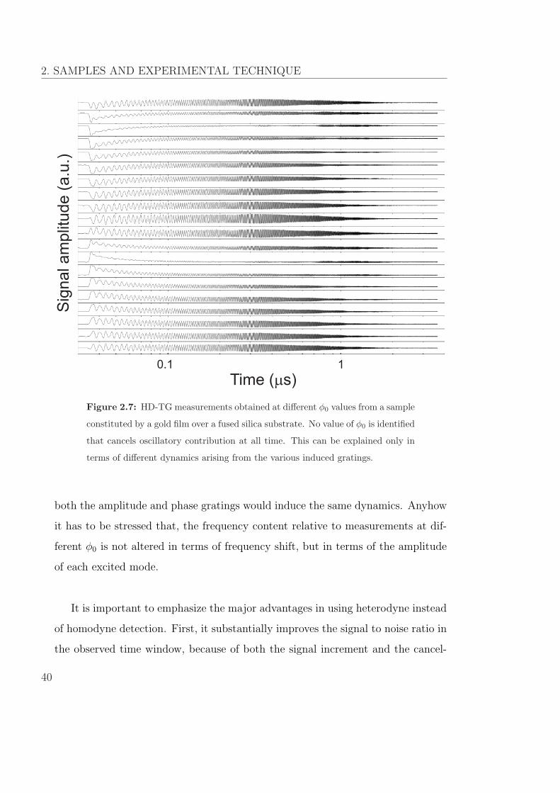
effective, and with different dynamics content as it can be understood from figure
2.7 where each of the 20 recorded signal is obtained at a phase φ0 according to
(2.18) and the phase φ0 is varied of π/10 from measurement to measurement in
order to cover the full phase angle 2π.
The fact that the various induced grating do not produce the same dynamics is
easily understood in terms of the absence of a phase term φ0 that cancels all the
oscillating contribution at all times, has it should results according to (2.18) if
39
2. SAMPLES AND EXPERIMENTAL TECHNIQUE
Time ( s)m
0.1 1
Sig
nal am
plit
ude (
a.u
.)
Figure 2.7: HD-TG measurements obtained at different φ0 values from a sample
constituted by a gold film over a fused silica substrate. No value of φ0 is identified
that cancels oscillatory contribution at all time. This can be explained only in
terms of different dynamics arising from the various induced gratings.
both the amplitude and phase gratings would induce the same dynamics. Anyhow
it has to be stressed that, the frequency content relative to measurements at dif-
ferent φ0 is not altered in terms of frequency shift, but in terms of the amplitude
of each excited mode.
It is important to emphasize the major advantages in using heterodyne instead
of homodyne detection. First, it substantially improves the signal to noise ratio in
the observed time window, because of both the signal increment and the cancel-
40

2.3 Samples
lation of the spurious signals which are not phase sensitive. Second, it enhances
the dynamic range since the recorded signal is directly proportional to signal field
instead of being proportional to its square. In the study of materials with a weak
scattering efficiency and complex responses, these features turn out to be of basic
importance. Furthermore, HD allows the measurement of the signal at very long
times, where the TG signals become very weak. Nevertheless, the effective real-
ization of such detection is quite difficult at optical frequencies. Indeed, to get an
interferometric phase stability between the diffracted and the local field is not a
simple experimental task, which explains why only very few HD-TG experiments
have been realized so far [37]. The introduction of the phase mask DOE in the
TG optical setup (see subsection 2.2.1) has considerably reduced the difficulties of
achieving heterodyne detection.
2.3 Samples
The sample that we characterized is a gold coated fused silica plate 2 mm thick.
An image of the sample is shown in Fig. 2.8(a). Two distinct area are clearly
distinguishable, an homogeneous region and a grooved one (5 × 5 mm). During
this work we have theoretically and experimentally characterized both regions.
In the rest of this thesis we will refer to those region as to the homogeneous
sample and the PC sample. The grooving displayed in Fig. 2.8(b) is obtained by
photolithographically defining a one dimensional squared optical grating in a layer
of photoresist coated on the glass surface. Reactive ion etching enables to transfer
the grating pattern to the glass surface. The remaining photoresist is then removed
with acetone. Finally, in order to excite surface acoustic waves, a thin gold film
is deposited on the surface by evaporation. In Fig. 2.8(c) a schematic view of the
grooving is given. The parameters peculiar of the lattice are: the lattice step a=5
41

2. SAMPLES AND EXPERIMENTAL TECHNIQUE
10 mm
Wigner-Seitz Cell
h
SiO2
Au
homogeneous
grooved
a
b
d
(a) (b)
(c)
Figure 2.8: (a) Macroscopic image of the sample. Two regions are identified:
the homogeneous and the grooved one. In (b) a SEM image of the grooved area
and in (c) a scheme corresponding to a cross section of the sample perpendicular
to the grooving.
µm, the duty cycle b/a=52%, the depth of the squared lattice d=0.860 µm and,
both for the homogeneous and grooved region, the film thickness h=0.130 µm.
The Wigner-Seitz cell is that chosen to simulate the band diagram of the sample
itself.
The values of mechanical parameters of both medium (Young’s modulus E,
Poisson’s ratio ν and density ρ) are plotted against a wide range of temperature
in Fig. 2.9. First row is that relative to gold’s parameters while second one is that
of fused silica.
We can relate these mechanical parameters to those present in the equation of
dynamics (1.10) (again the density ρ plus cl and ct, the longitudinal and transverse
42

2.3 Samples
0 400 800 120040
60
80
You
ng's
mod
ulus
(GP
a)
Temperature (K)300 600 900 1200
0.445
0.450
Poi
sson
's ra
tio
Temperature (K)200 400 600 800 1000
18800
19200
Den
sity
(kg/
m3 )
Temperature (K)
0 200 400 600 800 1000 1200 1400 1600
72
76
80
You
ng's
mod
ulus
(GP
a)
Temperature (K)200 400 600 800 1000 1200 1400 1600
0.16
0.17
0.18
0.19
Poi
sson
's ra
tio
Temperature (K)200 400 600 800 1000
2218
2220
Den
sity
(kg/
m3 )
Temperature (K)
Figure 2.9: First row: gold mechanical parameters as a function of temperature
over a wide range. Second row: fused silica mechanical parameters
velocity respectively) according to the following equations
cl =
√1
ρ
E(1− ν)
(1 + ν)(1− 2ν)(2.19)
ct =
√1
ρ
E
2(1 + ν)(2.20)
We performed our measurements at room temperature, however it has to be noted
that even a huge variation of 10 K around the room temperature do not signif-
icantly alters the mechanical parameters. Their values at room temperature are
43
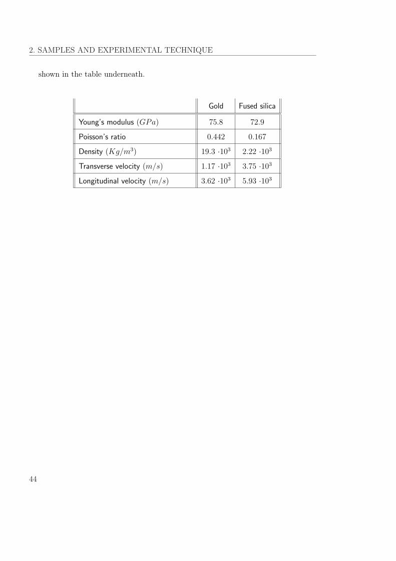
2. SAMPLES AND EXPERIMENTAL TECHNIQUE
shown in the table underneath.
Gold Fused silica
Young’s modulus (GPa) 75.8 72.9
Poisson’s ratio 0.442 0.167
Density (Kg/m3) 19.3 ·103 2.22 ·103
Transverse velocity (m/s) 1.17 ·103 3.75 ·103
Longitudinal velocity (m/s) 3.62 ·103 5.93 ·103
44
Chapter 3SIMULATIONS
A consistent part of this study has been directed towards the theoretical charac-
terization of the dispersion relation of the analyzed samples. In this chapter the
main characteristics of the software by which simulations has been realized will be
briefly introduced. The goodness of our simulations will be then tested in com-
parison with literature results [9] and a standard procedure for the eigenfrequency
analysis will be given. Finally the comparison between literature’s experimental
TG results regarding propagation of SAW in periodic surfaces (lacking of any sim-
ulation) [29] [30] will be compared to the simulations that have been performed
on those samples.
3.1 COMSOL Multiphysics c©
COMSOL Multiphysics (CM) is a commercial software. It consists of a simulation
environment that allows all steps in the modelling process (defining the geome-
try, specifying the physics, meshing, solving and then post-processing the results)
without any specific programming knowledge. It performs calculations of partial
differential equations (PDE) over complex domains performing a finite element
45

3. SIMULATIONS
analysis (FEA). FEA is a numerical technique to find approximate solutions to
PDE. The solution approach is based on transforming PDE into an approximating
system of ordinary differential equations, that are numerically stable and can be
solved with standard techniques.
Model set up is quick, thanks to a number of predefined modelling interfaces for
applications ranging from fluid flow and heat transfer to structural mechanics (that
of our interest) and electromagnetic analysis. Material properties, source terms
and boundary conditions can all be arbitrary functions of the dependent variables.
COMSOL Multiphysics operates as the primary tool for modelling needs. Its main
peculiarities are its versatility, flexibility and usability.
3.1.1 Structural mechanics module
This module is specialized in the analysis of components and subsystems where it
is necessary to evaluate structural deformations. Application modes in this module
solve stationary and dynamic models, perform eigenfrequency, parametric, quasi-
static and frequency-response analysis.
COMSOL Multiphysics includes four application modes for stress analysis and
general structural mechanics simulation:
• The Solid, Stress-Strain application mode (for 3D geometries)
• The Plane Stress application mode, applicable in volume bodies with one
dimension much smaller than the other two (realizes a 2D geometry)
• The Plane Strain application mode, usually applied in volume bodies with
one dimension (z in Fig. 3.1) much bigger than the other two (realizes a 2D
geometry)
• The Axial Symmetry Stress-Strain application mode (for 2D axisymmetric
geometries)
46
3.1 COMSOL Multiphysics c©
The last three cases are 2D simplifications of the full 3D equations. Simplifications
are valid under certain assumptions.
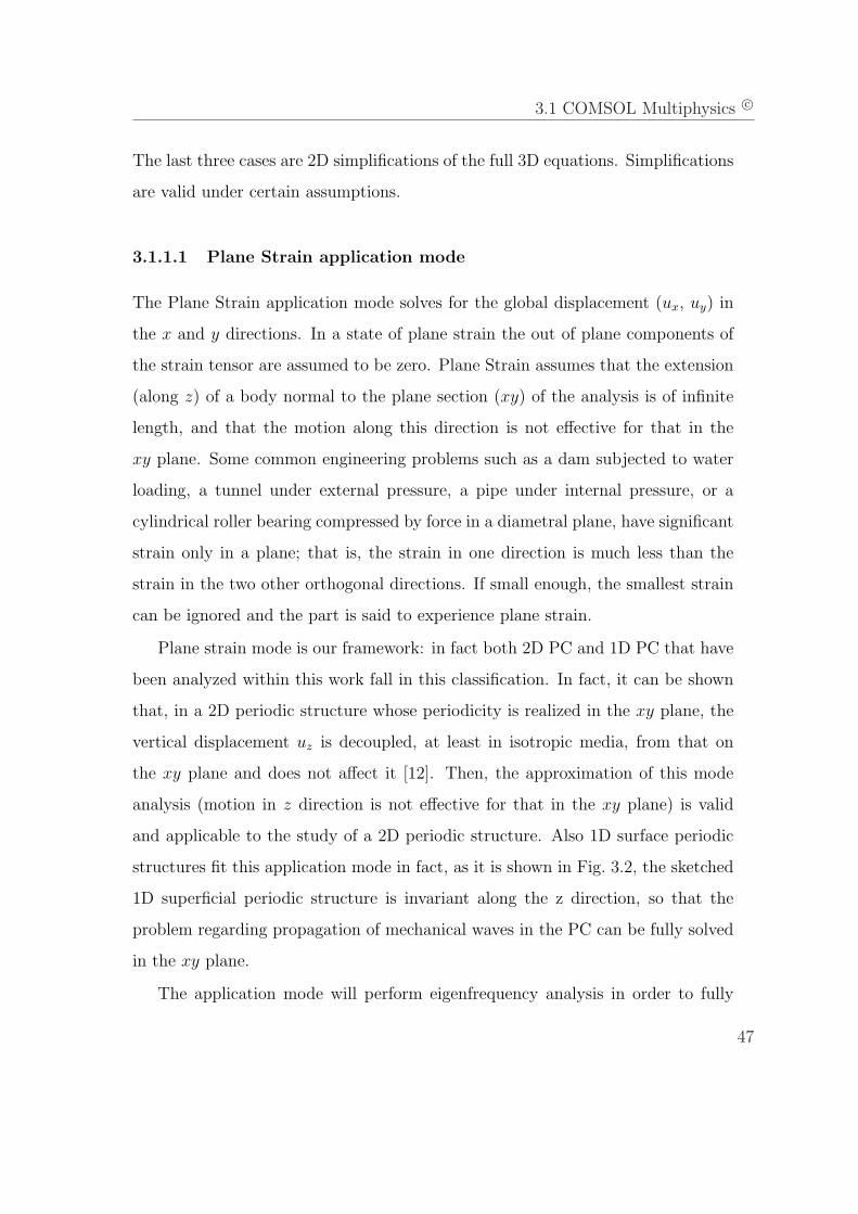
3.1.1.1 Plane Strain application mode
The Plane Strain application mode solves for the global displacement (ux, uy) in
the x and y directions. In a state of plane strain the out of plane components of
the strain tensor are assumed to be zero. Plane Strain assumes that the extension
(along z) of a body normal to the plane section (xy) of the analysis is of infinite
length, and that the motion along this direction is not effective for that in the
xy plane. Some common engineering problems such as a dam subjected to water
loading, a tunnel under external pressure, a pipe under internal pressure, or a
cylindrical roller bearing compressed by force in a diametral plane, have significant
strain only in a plane; that is, the strain in one direction is much less than the
strain in the two other orthogonal directions. If small enough, the smallest strain
can be ignored and the part is said to experience plane strain.
Plane strain mode is our framework: in fact both 2D PC and 1D PC that have
been analyzed within this work fall in this classification. In fact, it can be shown
that, in a 2D periodic structure whose periodicity is realized in the xy plane, the
vertical displacement uz is decoupled, at least in isotropic media, from that on
the xy plane and does not affect it [12]. Then, the approximation of this mode
analysis (motion in z direction is not effective for that in the xy plane) is valid
and applicable to the study of a 2D periodic structure. Also 1D surface periodic
structures fit this application mode in fact, as it is shown in Fig. 3.2, the sketched
1D superficial periodic structure is invariant along the z direction, so that the
problem regarding propagation of mechanical waves in the PC can be fully solved
in the xy plane.
The application mode will perform eigenfrequency analysis in order to fully
47

3. SIMULATIONS
ux
uy
Figure 3.1: Also 2D periodic structure can be solved in the plane strain mode:
along the z direction, invariant for translation, the displacement uz is decoupled
from that in the plane ux and uy [12].
ux
uy
Figure 3.2: Schematic draw of a 1D superficial PC. The sample is z direction
invariant. Once again the displacements ux and uy in the plane xy can be fully
calculated independently of the z dimension.
48
3.2 Standard procedure and software test
reconstruct the band diagram of the analyzed PC.
3.2 Standard procedure and software test
x
y
a
G
M X
x
y
a)
b)
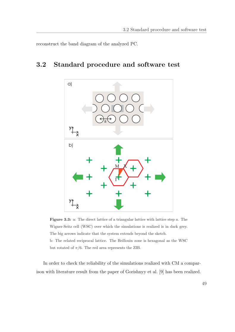
Figure 3.3: a: The direct lattice of a triangular lattice with lattice step a. The
Wigner-Seitz cell (WSC) over which the simulations is realized is in dark grey.
The big arrows indicate that the system extends beyond the sketch.
b: The related reciprocal lattice. The Brillouin zone is hexagonal as the WSC
but rotated of π/6. The red area represents the ZIB.
In order to check the reliability of the simulations realized with CM a compar-
ison with literature result from the paper of Gorishnyy et al. [9] has been realized.
49
3. SIMULATIONS
This section is organized as follows: first the procedure to realize the simulations
will be shown (the specific geometry that is presented here will be easily extendible
to other general cases), then a direct comparison of the simulated band diagrams
will be presented.
3.2.1 Setting up the simulation
Once that the appropriate structural mechanic module (plane stress) and applica-
tion mode (eigenfrequency analysis) have been chosen it’s time to concentrate on
the geometry of the system. The sample investigated in [9] consists of triangular
arrays of empty cylindrical holes in epoxy matrix (with a radius to lattice step
ratio of 0.33) and the relation dispersion to be characterized is that of bulk waves
propagating in the plane orthogonal to the cylinder axis with wave vector along
the ΓM direction of the irreducible Brillouin zone (ZIB). The first step is to de-
sign the Wigner-Seitz cell of the system under study (Draw menu) and assign the
appropriate materials to the domains trough the Physics/Subdomain Settings
menu. Until now no prescriptions have been given to the software about the pe-
riodicity of the system. This is realized imposing the displacement field to satisfy
the Bloch conditions on the boundary of the cell. In this particular case there
are three translation relative to three different direct lattice vectors which define
the translation from side 1 to side 4 (R14), side 2 to side 5 (R25) and side 6 to
side 3 (R63) where side 1 is chosen to be vertical side on the left and enumeration
proceeds clockwise.
How this informations are given to the software? This is realized substantially
in two steps. The first one consists in defining the opportune constants trough
Options/Constants menu (as in Fig. 3.5). The second is realized imposing the
Bloch conditions trough the Physics/Periodic Boundary Conditions menu. Here
side i is selected (be it 1, 2 or 6) and two constraints are defined: horizontal dis-
50
3.2 Standard procedure and software test
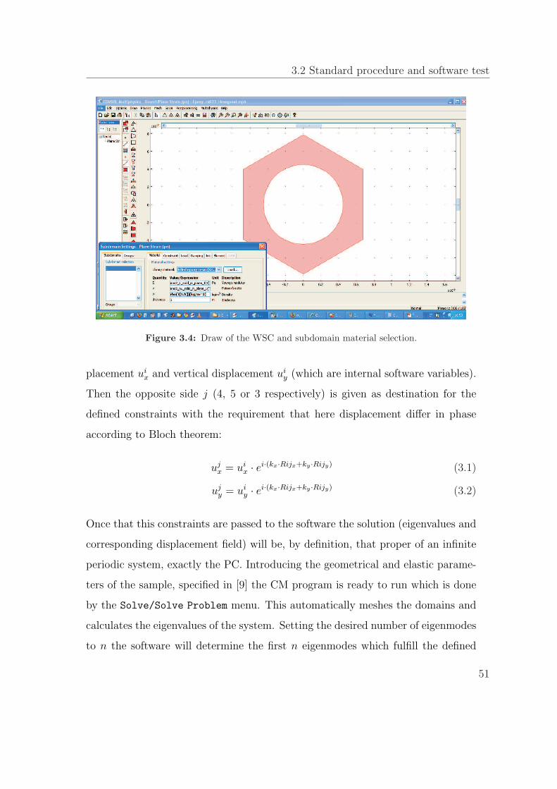
Figure 3.4: Draw of the WSC and subdomain material selection.
placement uix and vertical displacement ui
y (which are internal software variables).
Then the opposite side j (4, 5 or 3 respectively) is given as destination for the
defined constraints with the requirement that here displacement differ in phase
according to Bloch theorem:
ujx = ui
x · ei·(kx·Rijx+ky ·Rijy) (3.1)
ujy = ui
y · ei·(kx·Rijx+ky ·Rijy) (3.2)
Once that this constraints are passed to the software the solution (eigenvalues and
corresponding displacement field) will be, by definition, that proper of an infinite
periodic system, exactly the PC. Introducing the geometrical and elastic parame-
ters of the sample, specified in [9] the CM program is ready to run which is done
by the Solve/Solve Problem menu. This automatically meshes the domains and
calculates the eigenvalues of the system. Setting the desired number of eigenmodes
to n the software will determine the first n eigenmodes which fulfill the defined
51

3. SIMULATIONS
Figure 3.5: List of the constants defined by the user.
sample from the lower eigenfrequency mode. The CM program solves the equa-
tion of motion defining the eigenvalues and eigenvectors. The relative displacement
field are shown on the main prompt, ready to be postprocessed. Varying the wave
vector ky specified in the constants the relation dispersion over ΓM is obtained.
However, defining the appropriate wave vector in the constants, it is possible to
fully characterize the relation dispersion along all the boundaries of the ZIB as
it can be understood from Fig. 3.3 b. For example if interested in the dispersion
along ΓX it is sufficient to set ky=0 in the constants and vary the value of kx from
zero up to ‖ΓX‖ = 4π/3a with convenient stepping. Finally to investigate the XM
edge kx will be varied (keeping ky=0) between ‖ΓX‖ and ‖ΓX‖+‖XM‖ with the
opportune stepping.
Finally, before comparing CM simulated band diagram with literature, it is worth
52

3.2 Standard procedure and software test
k =0.9 My ° G
1st mode 2nd mode
Figure 3.6: Displacement field associated to the first (predominantly transverse)
and second (predominantly longitudinal) eigenmode. Colour scale represents the
total displacement (√
u2x + u2
y) in arbitrary units. Arrows stand for the displace-
ment field (also in arbitrary units).
noticing that plotted arrows in the first mode of Fig. 3.6 clearly manifest the
predominantly transverse character of this eigenmode (remember wave vector is
along y axis, vertical direction in figure), while, the second one is predominantly
longitudinal.
3.2.2 The comparison with literature
In Fig. 3.7 a comparison with some literature results is presented. The band
diagram characterized in [9], has been simulated by CM and compared with that
reported in [9]. Data from [9] are represented by open circles in Fig. 3.7, blue
(green) circles correspond to mainly transverse (longitudinal) modes, as stated in
53

3. SIMULATIONS
0.0 0.5 1.0 1.5 2.0 2.5 3.0
0
200
400
600
800
1000
1200
1400
Freq
uenc
y (M
Hz)
wave vector ( m-1)M
Figure 3.7: Comparison between band diagram present in [9] (open circles)
and CM simulations (dashed squares). Different colours within the same set of
simulations correspond to different states of polarization of the modes (see text).
the paper. The simulation realized with CM program using the previously reported
procedures is plotted with full dashed squares. Black (red) squares correspond to
mainly transverse (longitudinal) modes.
It has to be stressed that the agreement between our simulation and the data
from [9] is really satisfying. This staten, CM reveals itself as a reliable software
to perform such calculations and modelings. This has proven to be a fundamental
and innovative part of this Ph.D. thesis, since, to our knowledge, no scientific pub-
lications declaring the employment of this software were present when we started
to use it.
54
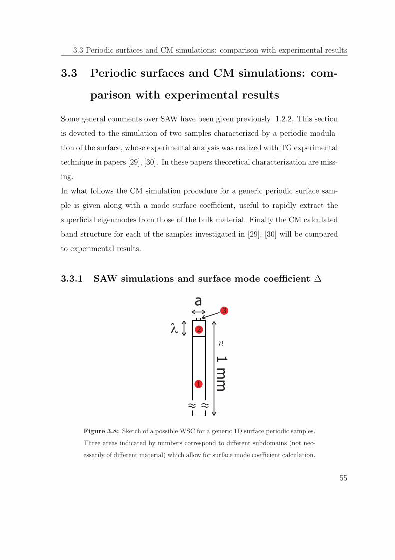
3.3 Periodic surfaces and CM simulations: comparison with experimental results
3.3 Periodic surfaces and CM simulations: com-
parison with experimental results
Some general comments over SAW have been given previously 1.2.2. This section
is devoted to the simulation of two samples characterized by a periodic modula-
tion of the surface, whose experimental analysis was realized with TG experimental
technique in papers [29], [30]. In these papers theoretical characterization are miss-
ing.
In what follows the CM simulation procedure for a generic periodic surface sam-
ple is given along with a mode surface coefficient, useful to rapidly extract the
superficial eigenmodes from those of the bulk material. Finally the CM calculated
band structure for each of the samples investigated in [29], [30] will be compared
to experimental results.
3.3.1 SAW simulations and surface mode coefficient ∆
l
a
1 m
m.
1
3
2
Figure 3.8: Sketch of a possible WSC for a generic 1D surface periodic samples.
Three areas indicated by numbers correspond to different subdomains (not nec-
essarily of different material) which allow for surface mode coefficient calculation.
55

3. SIMULATIONS
The simulation of a thick sample presenting a surface periodicity, as that shown
in Fig. 3.2 follows the same general procedure already presented. In such samples
we are mainly interested in the investigation of surface waves characteristics. Some
remarks are needed to make the scenario clearer.
The generic sample that we consider is a thick plate (say of a millimeter) with a
1D surface periodicity (some microns) realized on one of the two principal faces of
the plate itself. Here we are defining a generic sample structure that characterize
all the samples investigated in this thesis. As we will show, the simulation of the
real sample will require some modification of this generic structure.
The first step consists in the definition of the cross section of minimum periodicity
and the realization with CM Draw menu of the chosen WSC (whose choice is
obviously not unambiguous). In Fig. 3.8 we report a possible WSC for a generic
surface periodic sample: the vertical side is the thickness dimension of the plate
, while horizontal side correspond to the lattice step of the sample itself. Once
that the WSC is realized it is useful to define a depth limit from the profiled
surface of about λ (remembering the constants table defined in section 3.6, this
means 2π/kx since the wave vector is parallel to the surface) that identifies a
surface portion of the thick plate. Then three domains can be identified within
the WSC: 1 - deep bulk, 2 - superficial bulk and 3- surface. After that the integral
inti =∫∫
Diρ(
√u2
x + u2y)dx dy should be defined (by the Options/Integration
Coupling Variables menu) in each of the subdomains (with 1 < i < 3) in order
to properly weight the displacement associated to each domain. By means of this
integrals we define the surface mode coefficient given by ∆ = (int2 + int3)/(int1 +
int2 + int3). Only surface acoustic modes will have significantly non zero value of
this coefficient, so that plotting ∆ against the eigenmode number (remember that
CM determines n eigenvalues as specified by the user) will allow to immediately
identify surface eigenmodes from those of the bulk, instead of identifying them
56

3.3 Periodic surfaces and CM simulations: comparison with experimental results
plot after plot.
3.3.2 Periodically surface profiled homogeneous sample
The surface profiled sample that has been investigated in [29] is that shown in
Fig. 3.9 (a), (b). Substantially it consists of a silica plate with square-wave surface
profile, with an additional aluminum coating.
Figure 3.9: (a,b) SEM images of the surface profiled sample. The grating
period is 3µm, the depth 1.15µm. An aluminum film coating of 75 nm was
deposited on the sample surface to easily excite and detect SAW. (c,d) Disper-
sion of acoustic frequencies on the aluminum coated patterned (open symbols)
and unpatterned (closed symbols) surface of glass. Vertical dotted line in (c)
represents the band edge wave vector, while dashed line in (d) represents the
longitudinal bulk velocity.
57
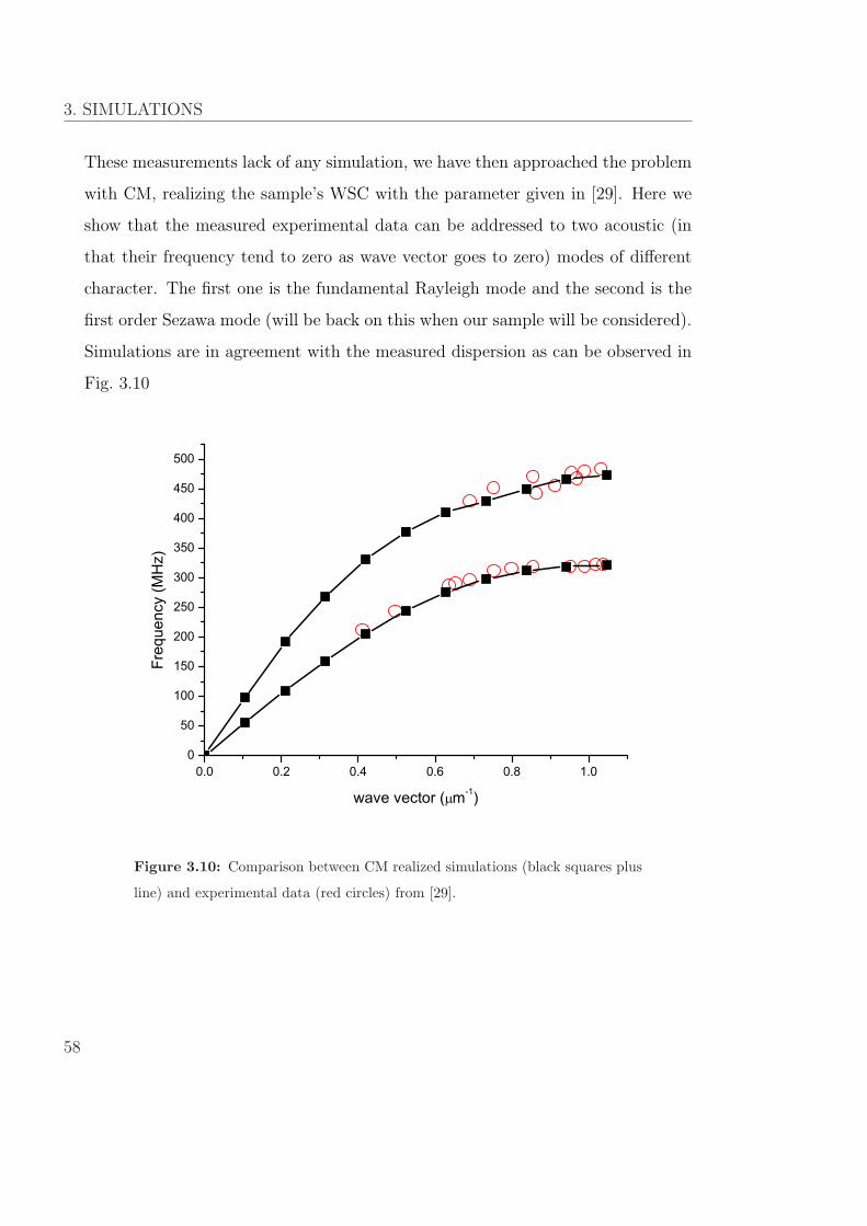
3. SIMULATIONS
These measurements lack of any simulation, we have then approached the problem
with CM, realizing the sample’s WSC with the parameter given in [29]. Here we
show that the measured experimental data can be addressed to two acoustic (in
that their frequency tend to zero as wave vector goes to zero) modes of different
character. The first one is the fundamental Rayleigh mode and the second is the
first order Sezawa mode (will be back on this when our sample will be considered).
Simulations are in agreement with the measured dispersion as can be observed in
Fig. 3.10
0.0 0.2 0.4 0.6 0.8 1.00
50
100
150
200
250
300
350
400
450
500
Freq
uenc
y (M
Hz)
wave vector ( m-1)
Figure 3.10: Comparison between CM realized simulations (black squares plus
line) and experimental data (red circles) from [29].
58

3.3 Periodic surfaces and CM simulations: comparison with experimental results
3.3.3 Periodic surface elastic composites sample
Figure 3.11: Top figure: a sketch of the sample from reference [30], and all
characteristic parameters. Bottom figure: (a) measured dispersion as a function
of induced wave vector, (b) dispersion as a function of reduced wave vector.
The surface composites sample of reference [30] consists of a periodic superficial
arrangement of silica and copper lines over a silicon bulk, as in Fig. 3.11. This
sample’s periodicity is realized by alternating materials of different elastic prop-
erties, while in that of reference [29] the periodicity was determined by surface
profiling. No theoretical band calculation is present in paper [30], then CM simu-
lations have been realized, realizing the appropriate WSC in accordance with the
parameters given in [30], and can be seen in Fig. 3.12. The agreement between the
experimental and simulated data is really satisfying. Three modes are observed.
While the first two have an acoustic character (once again in that frequency goes
to zero as wave vector goes to zero), contrarily the third mode does not reach zero
frequency for low wave vectors and is a flat “optical” mode (we name it “optical”
in analogy with diatomic chain). Finally it can be of interest to have a look at
the displacement field at the band edge (where the wavelength is twice the lattice
59
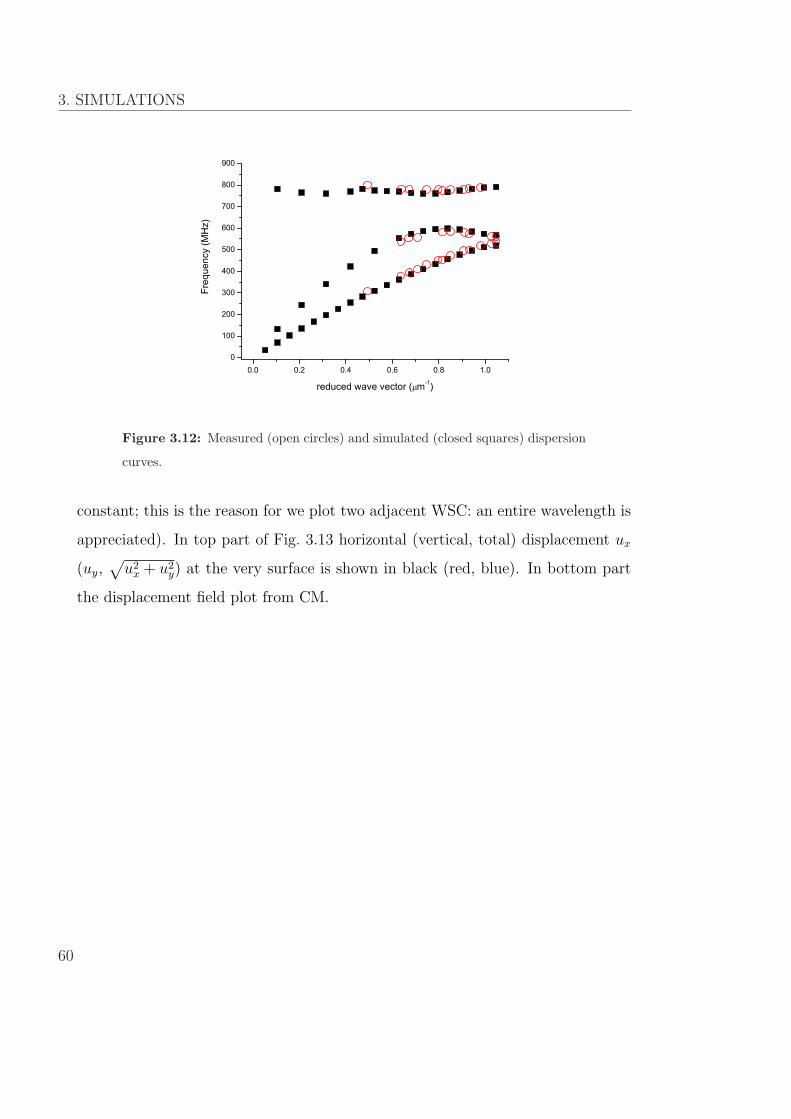
3. SIMULATIONS
0.0 0.2 0.4 0.6 0.8 1.00
100
200
300
400
500
600
700
800
900
Freq
uenc
y (M
Hz)
reduced wave vector ( m-1)
Figure 3.12: Measured (open circles) and simulated (closed squares) dispersion
curves.
constant; this is the reason for we plot two adjacent WSC: an entire wavelength is
appreciated). In top part of Fig. 3.13 horizontal (vertical, total) displacement ux
(uy,√
u2x + u2
y) at the very surface is shown in black (red, blue). In bottom part
the displacement field plot from CM.
60

3.3 Periodic surfaces and CM simulations: comparison with experimental results
Figure 3.13: Top: displacement at the very surface of the sample for the band
edge wave vector as a function of horizontal axis. From left to right: the first,
second and third order mode. Black line (red, blue) correspond to ux (uy,√u2
x + u2y). Bottom: plot from CM for each of the simulated mode. Colour
scale is for total displacement while arrows are displacement field.
61


Chapter 4RESULTS AND DISCUSSION
This concluding chapter concerns the main results obtained within this Ph.D.
thesis.
The results obtained both for the patterned and homogeneous region of the sample
will be presented. We will mainly focus on the great difference in the measured
dispersion relation between the two cases, and, in particular, great attention will
be devoted to the band diagram structure revealed and theoretically calculated for
the patterned region of the analyzed sample. Along with these main results other
results will be presented, such as the direct measurement of extraordinary slow
waves due to the surface profiling. During the discussion some key points (already
widely discussed in the preceding chapters) needed for a full comprehension will
be recalled.
4.1 Propagation in homogenous region and in
grooved region parallel to the grooves
Subject of our study are those surface waves which lay in the sagittal plane, by
definition that which contains both the normal to the surface and the wave vector.
63
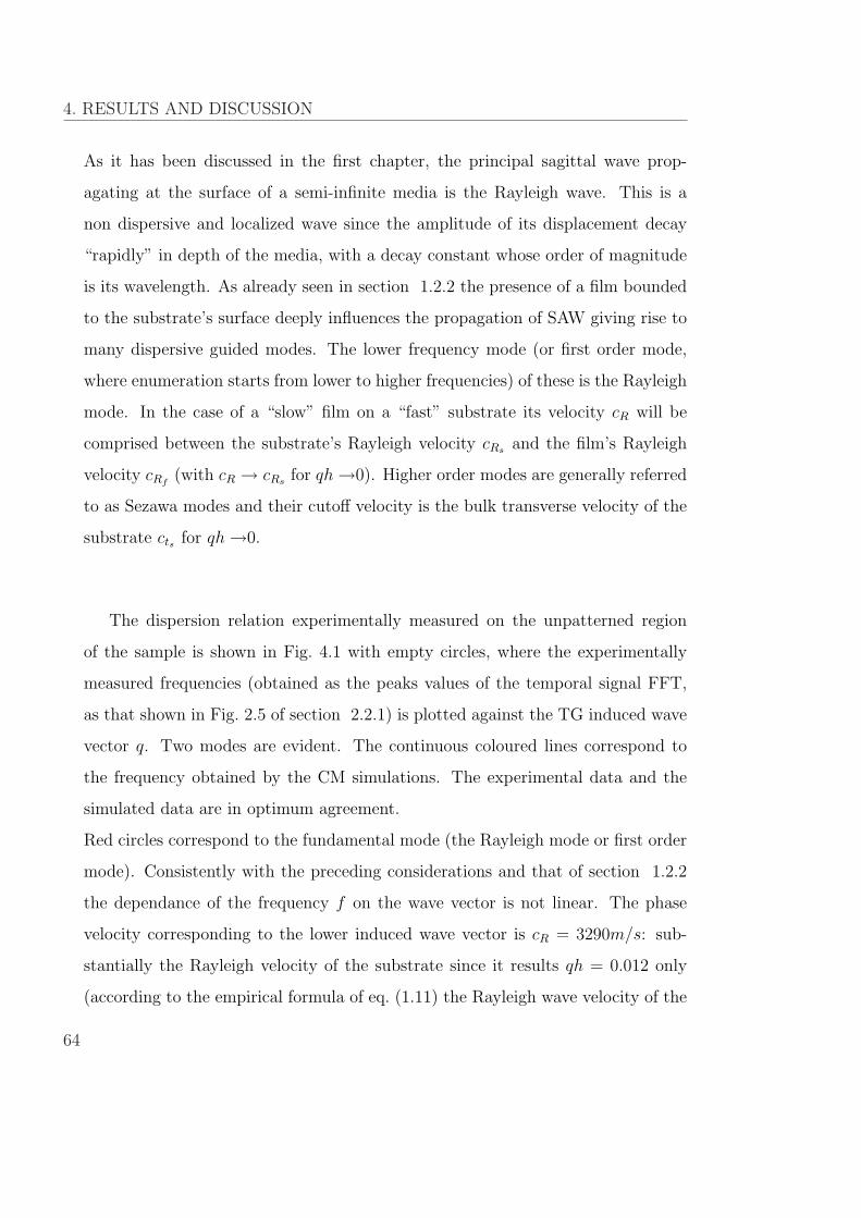
4. RESULTS AND DISCUSSION
As it has been discussed in the first chapter, the principal sagittal wave prop-
agating at the surface of a semi-infinite media is the Rayleigh wave. This is a
non dispersive and localized wave since the amplitude of its displacement decay
“rapidly” in depth of the media, with a decay constant whose order of magnitude
is its wavelength. As already seen in section 1.2.2 the presence of a film bounded
to the substrate’s surface deeply influences the propagation of SAW giving rise to
many dispersive guided modes. The lower frequency mode (or first order mode,
where enumeration starts from lower to higher frequencies) of these is the Rayleigh
mode. In the case of a “slow” film on a “fast” substrate its velocity cR will be
comprised between the substrate’s Rayleigh velocity cRs and the film’s Rayleigh
velocity cRf(with cR → cRs for qh →0). Higher order modes are generally referred
to as Sezawa modes and their cutoff velocity is the bulk transverse velocity of the
substrate cts for qh →0.
The dispersion relation experimentally measured on the unpatterned region
of the sample is shown in Fig. 4.1 with empty circles, where the experimentally
measured frequencies (obtained as the peaks values of the temporal signal FFT,
as that shown in Fig. 2.5 of section 2.2.1) is plotted against the TG induced wave
vector q. Two modes are evident. The continuous coloured lines correspond to
the frequency obtained by the CM simulations. The experimental data and the
simulated data are in optimum agreement.
Red circles correspond to the fundamental mode (the Rayleigh mode or first order
mode). Consistently with the preceding considerations and that of section 1.2.2
the dependance of the frequency f on the wave vector is not linear. The phase
velocity corresponding to the lower induced wave vector is cR = 3290m/s: sub-
stantially the Rayleigh velocity of the substrate since it results qh = 0.012 only
(according to the empirical formula of eq. (1.11) the Rayleigh wave velocity of the
64
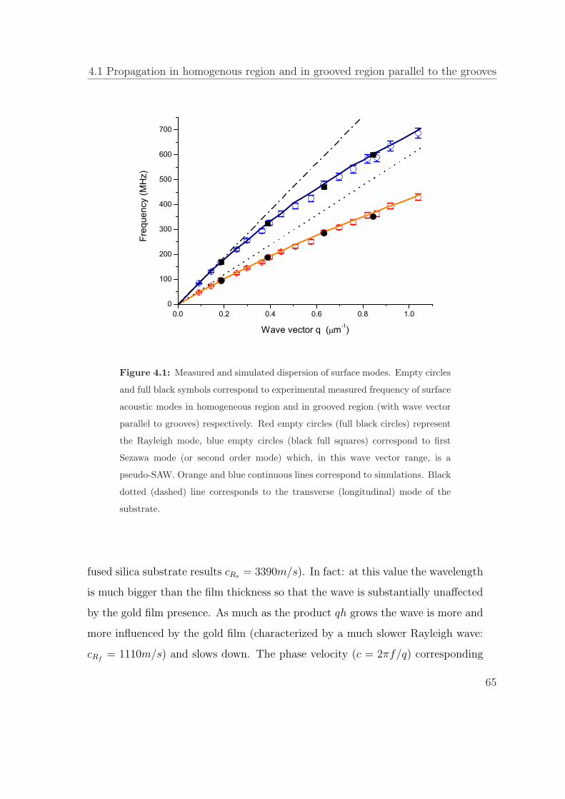
4.1 Propagation in homogenous region and in grooved region parallel to the grooves
0.0 0.2 0.4 0.6 0.8 1.00
100
200
300
400
500
600
700
Freq
uenc
y (M
Hz)
Wave vector q ( m-1)
Figure 4.1: Measured and simulated dispersion of surface modes. Empty circles
and full black symbols correspond to experimental measured frequency of surface
acoustic modes in homogeneous region and in grooved region (with wave vector
parallel to grooves) respectively. Red empty circles (full black circles) represent
the Rayleigh mode, blue empty circles (black full squares) correspond to first
Sezawa mode (or second order mode) which, in this wave vector range, is a
pseudo-SAW. Orange and blue continuous lines correspond to simulations. Black
dotted (dashed) line corresponds to the transverse (longitudinal) mode of the
substrate.
fused silica substrate results cRs = 3390m/s). In fact: at this value the wavelength
is much bigger than the film thickness so that the wave is substantially unaffected
by the gold film presence. As much as the product qh grows the wave is more and
more influenced by the gold film (characterized by a much slower Rayleigh wave:
cRf= 1110m/s) and slows down. The phase velocity (c = 2πf/q) corresponding
65
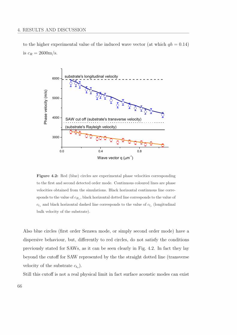
4. RESULTS AND DISCUSSION
to the higher experimental value of the induced wave vector (at which qh = 0.14)
is cR = 2600m/s.
0.0 0.4 0.8
3000
4000
5000
6000
(substrate's Rayleigh velocity)
substrate's longitudinal velocity
Pha
se v
eloc
ity (m
/s)
Wave vector q ( m-1)
SAW cut off (substrate's transverse velocity)
Figure 4.2: Red (blue) circles are experimental phase velocities corresponding
to the first and second detected order mode. Continuous coloured lines are phase
velocities obtained from the simulations. Black horizontal continuous line corre-
sponds to the value of cRs , black horizontal dotted line corresponds to the value of
cts and black horizontal dashed line corresponds to the value of cls (longitudinal
bulk velocity of the substrate).
Also blue circles (first order Sezawa mode, or simply second order mode) have a
dispersive behaviour, but, differently to red circles, do not satisfy the conditions
previously stated for SAWs, as it can be seen clearly in Fig. 4.2. In fact they lay
beyond the cutoff for SAW represented by the the straight dotted line (transverse
velocity of the substrate cts).
Still this cutoff is not a real physical limit in fact surface acoustic modes can exist
66

4.1 Propagation in homogenous region and in grooved region parallel to the grooves
also beyond this. This waves are known in literature as pseudosurface acoustic
waves (PSAW) or leaky waves in that they radiate energy to the substrate [46,47].
The nature of these PSAW differs from that under the cutoff. As a matter of fact
the displacement field and modulus has a different behaviour from those of “pure”
SAWs (under the cutoff) as it will be shown in the following. The only physical cut
off is given by the segmented straight line representing the substrate’s longitudinal
mode. We observe that for low q values the phase velocity is approximately that
of the longitudinal acoustic mode in the bulk of the substrate as from Fig. 4.2.
How do these modes look like? The simulation allow us to visualize the dis-
X
Y
1st mode 2nd mode
max
min
Figure 4.3: Displacement field (a.u.) associated to first and second mode is
vectorially represented by the arrows, total displacement is in colour scale (legend
shown on the right). The x dimension is equal to that of the simulated wavelength
(λ = 10µm → q = 0.628µm−1).
placement field of each mode, and this turns to be an optimum tool to have a
deeper insight over the character of the surface modes. Let’s make some general
67

4. RESULTS AND DISCUSSION
comments over the two modes displayed in Fig. 4.3 (what follow holds for all the
investigated wave vector range), where, arrows represent the displacement field in
vectorial form, and total displacement is shown in colour scale. The x direction
extension shown in the figure is equal to that of the simulated wavelength (in this
particular case λ = 10µm). First of all: total displacement (√
u2x + u2
y) clarifies
the surface character of these modes, in fact the maxima are located at the very
surface of the simulated sample. Another information is retrieved by means of the
total displacement: the different decay in depth of the two modes. Plotting the
decay of ux, uy and√
u2x + u2
y as a function of depth in the material (Fig. 4.4)
the different behaviour of the two surface modes is evident. The first mode de-
0 10 20 30
(2ndmode)
(1st mode)
ux
uy
(u2x+u2
y)0.5
Dis
plac
emen
t (a.
u.)
Y depth ( m)
=10 m
0 10 20 30
0
0
Figure 4.4: Displacement ux, uy and total displacement√
u2x + u2
y as a function
of depth.
cays within a depth y ∼ λ and is already approximately zero when y ∼ 2λ. This
68
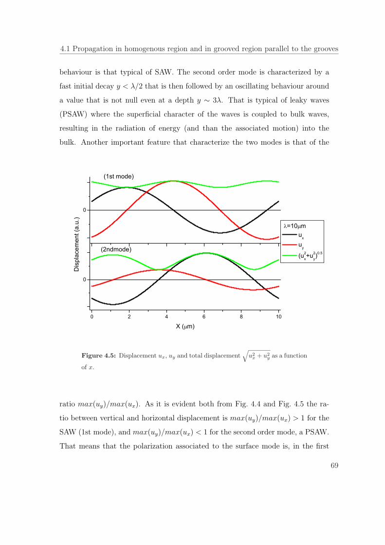
4.1 Propagation in homogenous region and in grooved region parallel to the grooves
behaviour is that typical of SAW. The second order mode is characterized by a
fast initial decay y < λ/2 that is then followed by an oscillating behaviour around
a value that is not null even at a depth y ∼ 3λ. That is typical of leaky waves
(PSAW) where the superficial character of the waves is coupled to bulk waves,
resulting in the radiation of energy (and than the associated motion) into the
bulk. Another important feature that characterize the two modes is that of the
0 2 4 6 8 10
0
0
=10 m u
x
uy
(u2x+u2
y)0.5
Dis
plac
emen
t (a.
u.)
X ( m)
(1st mode)
(2ndmode)
Figure 4.5: Displacement ux, uy and total displacement√
u2x + u2
y as a function
of x.
ratio max(uy)/max(ux). As it is evident both from Fig. 4.4 and Fig. 4.5 the ra-
tio between vertical and horizontal displacement is max(uy)/max(ux) > 1 for the
SAW (1st mode), and max(uy)/max(ux) < 1 for the second order mode, a PSAW.
That means that the polarization associated to the surface mode is, in the first
69

4. RESULTS AND DISCUSSION
case, that of an ellipsis with main axes along the normal to the surface, while in
the second case is that of an ellipsis with main axis along the x axis, that of the
wave vector associated to the modes. So, for the first mode the motion is mainly
transverse, and for the second is mainly of longitudinal character, as it is evident
considering Fig. 4.3.
Finally we want to underline that in both cases (first and second order mode), both
displacements (ux and uy) evolution along the x direction (Fig. 4.5) are sinusoidal
and have a relative phase difference of π/2.
The elusive nature of PSAW requires an excellent signal to noise ratio in order
to detect them experimentally, in fact as one of main contribution to the signal
of TG experiment is associated to the vertical displacement whereas their associ-
ated displacement is predominantly longitudinal (horizontal displacement ux) the
detection of such waves can be a hard task.
It is interesting to define a SAW likeness coefficient α =∫ ∫ 2π/q
0v2/u2dxdy for
these PSAW (leaky waves): in Fig. 4.6 (top) it can be observed that as the wave
vector increases the value of α also raises which implies that the wave tends to
assume the mainly vertical character of those modes under the cutoff. This trend
has an experimental confirmation as shown in Fig. 4.6 (bottom), in fact, given
the predominantly vertical displacement’s sensitivity of the experiment, by com-
paring the amplitude of the PSAW peak relative to q=0.092 µm−1 (in black) and
to q=1.04 µm−1. As expected the intensity of this peak (each spectra has been
normalized so that the maximum of the first order peak is unity) is higher for the
bigger wave vector, which is consistent with the observation over α.
Finally it is worth noticing that it is not surprising that we observe one only
“pure” SAW in fact the qh range we explore is really narrow and close to zero
0.012 < qh < 0.14 (dashed region shown in Fig. 4.7), which is the analogue of
70
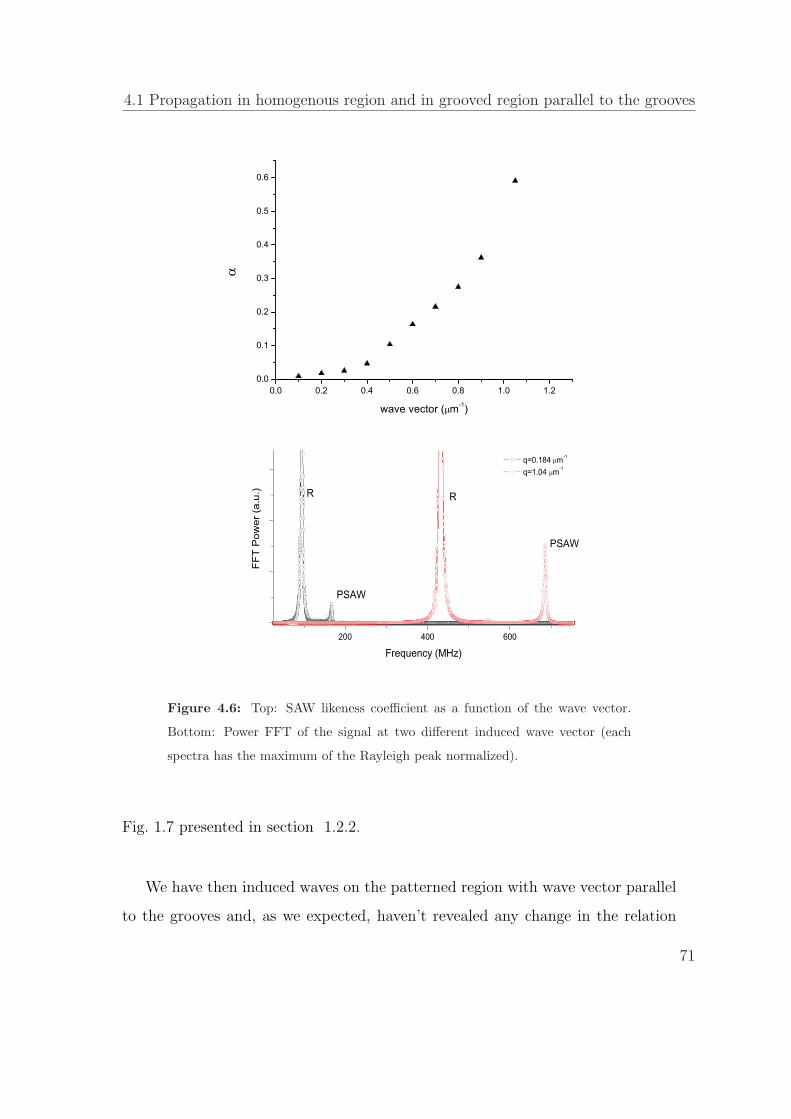
4.1 Propagation in homogenous region and in grooved region parallel to the grooves
0.0 0.2 0.4 0.6 0.8 1.0 1.20.0
0.1
0.2
0.3
0.4
0.5
0.6
wave vector ( m-1)
200 400 600
q=0.184 m-1
q=1.04 m-1
Frequency (MHz)
FFT
Pow
er (a
.u.)
PSAW
R R
PSAW
Figure 4.6: Top: SAW likeness coefficient as a function of the wave vector.
Bottom: Power FFT of the signal at two different induced wave vector (each
spectra has the maximum of the Rayleigh peak normalized).
Fig. 1.7 presented in section 1.2.2.
We have then induced waves on the patterned region with wave vector parallel
to the grooves and, as we expected, haven’t revealed any change in the relation
71

4. RESULTS AND DISCUSSION
0 2 4 6 8 10
1000
2000
3000
4000
5000
6000
phas
e ve
loci
ty (m
/s)
qh (h=film thickness, q=wave vector)
SAW cut off
Substrate's bulk longitudinal
Figure 4.7: Phase velocity as a function of the product of the wave vector q
and the film thickness h, experimental data are represented with circles, simula-
tions are shown as continuous line. Shaded region is the experimentally explored
region.
dispersion (see Fig. 4.1) of the two modes (black circles and square respectively):
the wave do not sense the surface structure as long as it propagates parallel to
grooves since, being contained in the sagittal plane, no periodicity is present along
this plane. That staten, please note that, when in the following we will refer to
the homogeneous data also the case of propagation in the patterned sample with
wave vector parallel to grooves will be implied.
72
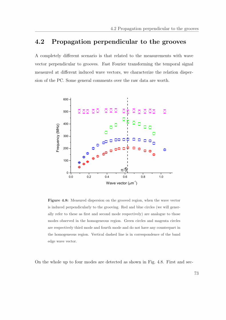
4.2 Propagation perpendicular to the grooves
4.2 Propagation perpendicular to the grooves
A completely different scenario is that related to the measurements with wave
vector perpendicular to grooves. Fast Fourier transforming the temporal signal
measured at different induced wave vectors, we characterize the relation disper-
sion of the PC. Some general comments over the raw data are worth.
0.0 0.2 0.4 0.6 0.8 1.00
100
200
300
400
500
600
Freq
uenc
y (M
Hz)
Wave vector ( m-1)
5
Figure 4.8: Measured dispersion on the grooved region, when the wave vector
is induced perpendicularly to the grooving. Red and blue circles (we will gener-
ally refer to these as first and second mode respectively) are analogue to those
modes observed in the homogeneous region. Green circles and magenta circles
are respectively third mode and fourth mode and do not have any counterpart in
the homogeneous region. Vertical dashed line is in correspondence of the band
edge wave vector.
On the whole up to four modes are detected as shown in Fig. 4.8. First and sec-
73
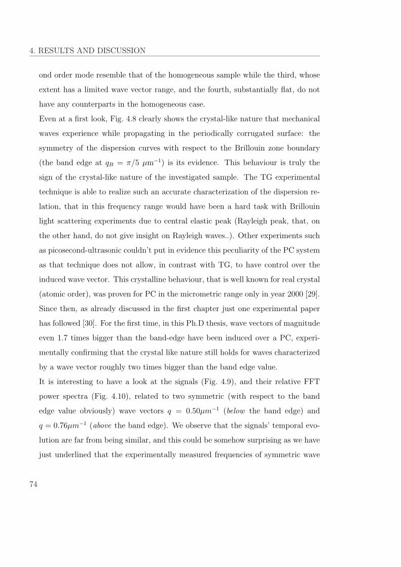
4. RESULTS AND DISCUSSION
ond order mode resemble that of the homogeneous sample while the third, whose
extent has a limited wave vector range, and the fourth, substantially flat, do not
have any counterparts in the homogeneous case.
Even at a first look, Fig. 4.8 clearly shows the crystal-like nature that mechanical
waves experience while propagating in the periodically corrugated surface: the
symmetry of the dispersion curves with respect to the Brillouin zone boundary
(the band edge at qB = π/5 µm−1) is its evidence. This behaviour is truly the
sign of the crystal-like nature of the investigated sample. The TG experimental
technique is able to realize such an accurate characterization of the dispersion re-
lation, that in this frequency range would have been a hard task with Brillouin
light scattering experiments due to central elastic peak (Rayleigh peak, that, on
the other hand, do not give insight on Rayleigh waves..). Other experiments such
as picosecond-ultrasonic couldn’t put in evidence this peculiarity of the PC system
as that technique does not allow, in contrast with TG, to have control over the
induced wave vector. This crystalline behaviour, that is well known for real crystal
(atomic order), was proven for PC in the micrometric range only in year 2000 [29].
Since then, as already discussed in the first chapter just one experimental paper
has followed [30]. For the first time, in this Ph.D thesis, wave vectors of magnitude
even 1.7 times bigger than the band-edge have been induced over a PC, experi-
mentally confirming that the crystal like nature still holds for waves characterized
by a wave vector roughly two times bigger than the band edge value.
It is interesting to have a look at the signals (Fig. 4.9), and their relative FFT
power spectra (Fig. 4.10), related to two symmetric (with respect to the band
edge value obviously) wave vectors q = 0.50µm−1 (below the band edge) and
q = 0.76µm−1 (above the band edge). We observe that the signals’ temporal evo-
lution are far from being similar, and this could be somehow surprising as we have
just underlined that the experimentally measured frequencies of symmetric wave
74
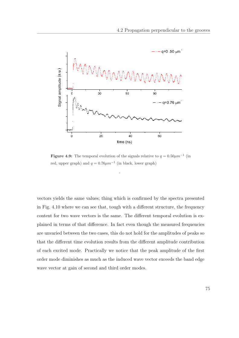
4.2 Propagation perpendicular to the grooves
Sig
na
l a
mp
litu
de
Figure 4.9: The temporal evolution of the signals relative to q = 0.50µm−1 (in
red, upper graph) and q = 0.76µm−1 (in black, lower graph)
.
vectors yields the same values; thing which is confirmed by the spectra presented
in Fig. 4.10 where we can see that, tough with a different structure, the frequency
content for two wave vectors is the same. The different temporal evolution is ex-
plained in terms of that difference. In fact even though the measured frequencies
are unvaried between the two cases, this do not hold for the amplitudes of peaks so
that the different time evolution results from the different amplitude contribution
of each excited mode. Practically we notice that the peak amplitude of the first
order mode diminishes as much as the induced wave vector exceeds the band edge
wave vector at gain of second and third order modes.
75

4. RESULTS AND DISCUSSION
Figure 4.10: The FFT power spectrum of the signals reveals that the frequency
content is, within the errors, the same
.
Given the crystalline behaviour, it is helpful to plot the dispersion curves ver-
sus the reduced wave number as in Fig. 4.11. The measured dispersion is consis-
tent with the simulations, continuous lines in Fig. 4.11, that we realized over the
Wigner-Seitz cell. In particular we want to stress that simulations of eigenmodes
allow for direct visualization of the associated displacement field, which will result
helpful in order to address the specific peculiarity of each mode. Both the data
and simulations show a separation of about 70 MHz at the band edge between the
first and second mode, anyhow this is not a band gap in the density of states, as
the second order mode bends down in frequency and overlap with this. Two real
76
4.2 Propagation perpendicular to the grooves
0.0 0.2 0.4 0.60
100
200
300
400
500
600
Freq
uenc
y (M
Hz)
Reduced wave vector ( m-1)
Figure 4.11: The data have been reduced to the first Brillouin zone. Contin-
uous coloured lines represent the simulated dispersion curves for the PC, folded
dispersion curves of the homogeneous sample (Rayleigh and Sezawa mode) are re-
plotted as lines (dot-dash and dot-dot-dash respectively), black dotted (dashed)
line correspond to the bulk transverse (longitudinal) mode in the substrate.
band gap are observed: one between the second and the third mode of approxi-
mately 55 MHz and the other between the third and the fourth mode of about 80
MHz. Some more words about the band gaps are needed, in fact we would have
expected a much larger band gap inside the Brillouin zone. This, as observed by
Maznev in [30], should have originated as a result of the “avoided crossing” be-
tween the homogeneous region Sezawa and zone folded Rayleigh modes (re-plotted
in Fig. 4.11 as dash-dot-dot and dash-dot lines respectively). Its frequency gap
would have been of about 220 MHz. A more detailed analysis of some analogue
77

4. RESULTS AND DISCUSSION
0.0 0.2 0.4 0.6103
Pha
se v
eloc
ity (m
/s)
Reduced wave vector ( m-1)
104
Figure 4.12: Phase velocities versus wave vector in the reduced zone scheme.
Red, blue, green and magenta circles correspond to first, second, third and fourth
mode respectively. Only the fourth mode phase velocity extends beyond the
longitudinal bulk velocity of the substrate. Dotted (dashed) line corresponds to
transverse (longitudinal) bulk phase velocity of the substrate.
samples where only pure SAW are excited (say the same sample with a thicker
film) would help to have a deeper comprehension of this phenomenon.
In Fig. 4.12 we plot the phase velocities deduced from dispersion relation in
the reduced zone scheme. We observe that the second order mode (blue circles)
cross the SAW cutoff (dotted horizontal line) at a value q ∼ 0.44µm−1.
The third order mode starts to be detected at a reduced wave vector value of
q ∼ 0.33µm−1 with a velocity which is that of the longitudinal bulk velocity
(dashed horizontal line), as much as the second order mode does at lower q values.
78
4.2 Propagation perpendicular to the grooves
We wonder if this third order mode is somehow to be attributed to a frequency
lowering (induced by the surface structuring) of the third order mode present in
the homogeneous simulation shown in Fig. 4.7. In fact, two interpretation of the
nature (apart its undoubted PSAW character) of this mode are possible: whether
it is an optical mode (where the word optical is used in analogy with the optical
mode of a diatomic chain) or it is an acoustic mode (meaning that its frequency
tends to zero as the wave vector tends to zero). The fact that we detect it exactly
in correspondence of the longitudinal bulk values let us be in favour of the latter
hypothesis, since, if it would be an optical mode, no restriction would apply to its
phase velocity.
Finally the fourth mode shows an impressive phase velocity well above that of the
longitudinal bulk velocity and its nature is evidently not acoustic.
Comparing the dispersion relation of the homogeneous sample with the first two
observed modes (Fig. 4.11) it is evident the importance that metamaterial could
cover in order to manipulate the mechanical parameters. In fact from the con-
stituent materials point of view, nothing is changed with respect to the homoge-
neous case. It is just the realization geometry that alters so much the effective
mechanical parameters, so that, for example, the second order mode, that had a
PSAW character in the homogeneous sample throughout all the investigated wave
vector range, becomes a SAW, in the PC, already at q = 0.44µm−1 and its fre-
quency at the band edge is roughly half of that of the homogeneous sample at
the same wave vector (qBE = 0.628µm−1). Engineering the design would result in
extracting the desired properties from bulk materials.
4.2.1 Rayleigh and Sezawa mode analysis
Lets now turn the attention on the first (Rayleigh) and second order (Sezawa)
mode. These are the analogue of those observed in the homogeneous region. The
79

4. RESULTS AND DISCUSSION
l=12.6 mm
l=40 mm
-1
-1
q m=0.50 m
q m=0.157 m
Figure 4.13: Displacement field associated to the second order at different wave
vector. Bottom: displacement field characteristic of PSAW for q = 0.157µm−1.
Top: SAW characteristic displacement field forq = 0.5µm−1.
effect of the surface structuring is to lower the frequency of both modes. The
two modes flatten as the wave vector tends to the band edge, so that their group
velocity reaches a null value leading to non propagative modes, we will consider
this in section 4.2.3.
As already said the second mode changes its superficial character along the
wave vector span at q = 0.44µm−1. It is a PSAW for wave vectors under this
value and become a SAW for wave vectors above this value. It can be instructive
80
4.2 Propagation perpendicular to the grooves
to plot its displacement field for the two cases (Fig. 4.13). Bottom part shows
a mainly longitudinal displacement field, and a not at rest condition in depth of
the material, that is typical of PSAW. By the way there are many similarities to
that commented in the homogeneous sample section 4.1. This is not surprising in
fact the wavelength is eight times the lattice step, then much bigger than both the
depth of the grooving and the lattice step itself. Top part of Fig. 4.13 shows on
the contrary a typical SAW displacement field: it is mainly transverse as testified
by the arrows, and no motion in the depth is present. A supplementary comment
over this displacement field may be worth. In fact it may be surprising that the
displacement field does not repeat periodically with the wavelength. It is not,
in fact, at q = 0.5µm−1 the wavelength is not a multiple of the lattice step, it
then follows that considering two points at the same depth and at a distance
λ they won’t be in the same relative position with respect to the cell. Then
the displacement associated to the two points will be differently affected by the
structure, so that the displacement doesn’t have the wavelength periodicity. This
can be easily understood in terms of the following arguments: the simulation
realizes the displacement field uq(r). So that the solution at a point r + R, where
R is a generic direct lattice vector will differ by a phase according to Bloch theorem
uq(r + R) = uq(r)e−i(q·R) (4.1)
To clarify the above statements we plot in bottom part of Fig. 4.14 the horizontal
(black) and vertical (red) displacement (at a fixed depth in the very proximity of
the surface) as a a function of the x axis for the wave vector q1 = 0.157µm−1,
and in bottom of Fig. 4.15 the same quantities for the wave vector q2 = 0.5µm−1.
From Fig. 4.14 we immediately see that for the lower wave vector the horizon-
tal displacement is predominating over the vertical displacement consistently with
its PSAW character, while the inverse hold in Fig. 4.15 for q2 (consistently with
its SAW character). Moreover the horizontal displacement for the wave vector
81

4. RESULTS AND DISCUSSION
0 100 200 300 400 500
Dis
plac
emen
t (a.
u.)
X Axis ( m)
0.0 0.1 0.2 0.3 0.4 0.5 0.6
FFT
Pow
er (a
.u.)
1/ m-1
Figure 4.14: Bottom: Displacement components at q1 = 0.157µm−1 as a func-
tion of X direction. In black (red) horizontal (vertical) displacement. The peri-
odicity is well defined by the associated wavelength and correspond to eight times
the lattice step (40µm). Top: Corresponding Spatial FFT. Both horizontal and
vertical displacement have a principal peak at 2π/q1, the peak at higher spatial
frequency corresponds to the symmetric wave vector q1′(see text).
q1 (corresponding to a wavelength λ = 40µm) is substantially a pure sinusoidal
function (with period λ) as it can be seen from its associated spatial FFT power
shown in top part of Fig. 4.14,confirming that the surface structuring substan-
tially doesn’t affect the horizontal displacement at such long wavelength. Also the
vertical displacement has a well defined period but, on the other hand, shows a
second contribution in the spectra since it is the vertical displacement that is more
82
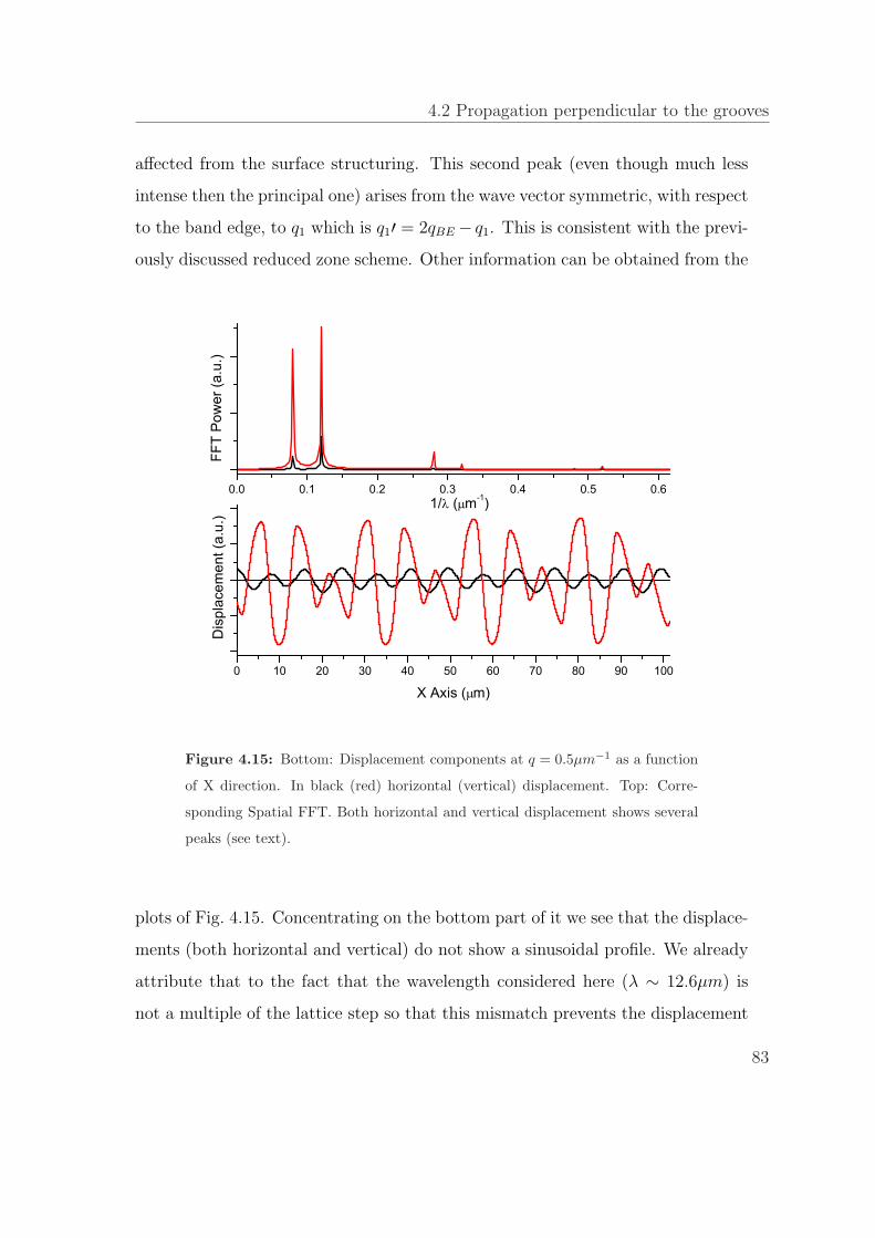
4.2 Propagation perpendicular to the grooves
affected from the surface structuring. This second peak (even though much less
intense then the principal one) arises from the wave vector symmetric, with respect
to the band edge, to q1 which is q1′ = 2qBE − q1. This is consistent with the previ-
ously discussed reduced zone scheme. Other information can be obtained from the
0 10 20 30 40 50 60 70 80 90 100
Dis
plac
emen
t (a.
u.)
X Axis ( m)
0.0 0.1 0.2 0.3 0.4 0.5 0.6
FFT
Pow
er (a
.u.)
1/ ( m-1)
Figure 4.15: Bottom: Displacement components at q = 0.5µm−1 as a function
of X direction. In black (red) horizontal (vertical) displacement. Top: Corre-
sponding Spatial FFT. Both horizontal and vertical displacement shows several
peaks (see text).
plots of Fig. 4.15. Concentrating on the bottom part of it we see that the displace-
ments (both horizontal and vertical) do not show a sinusoidal profile. We already
attribute that to the fact that the wavelength considered here (λ ∼ 12.6µm) is
not a multiple of the lattice step so that this mismatch prevents the displacement
83
4. RESULTS AND DISCUSSION
field from having the wavelength periodicity. Another interesting feature is seen
in top part of Fig. 4.15. In fact here, not only the two contribution from q2 and
its symmetric wave vector q2′ = 2qBE − q2 are observed, but also other are peaks
are present. Where do they arise from? This peaks are the contributions of the
Bloch harmonics relative to q2 and q2′. In fact, the displacement, say the vertical
displacement uy (but the same holds for the horizontal), of a mode propagating
along the x axis with wave vector q can be represented, dropping the temporal
term, by a superposition of Bloch harmonics [30]
uy =n=+∞∑n=−∞
Anei[(q+ 2πna
)x) (4.2)
whose peaks are those observed in top part of Fig. 4.15.
4.2.2 Structures of modes at the band edge
The plots shown in Fig. 4.16 are instructive, for we can appreciate the different
character of each of the detected modes. From this plots we extrapolated cross-
sectional displacement field, along both the horizontal (Fig. 4.16), and the vertical
direction (Fig. 4.17). We clearly distinguish the SAW character of the first and
second order mode. The third mode character is more ambiguous. In fact it is
by definition a PSAW (its phase velocity is above the threshold, see Fig. 4.12)
still both its decay profile and the ratio between the amplitude of the longitudinal
and horizontal oscillation do not fully confirm this thesis. In fact even tough the
non zero value around which it oscillates in deep bulk is that typical of PSAW,
the initial decay is not so “fast” as that typical of leaky waves, as shown for the
homogeneous sample, but resemble that of first and second order mode, two pure
SAW. Finally the ratio between the maximum horizontal and vertical displace-
ment is that characteristic of SAW, as a matter of fact the polarization is mainly
transverse.
84
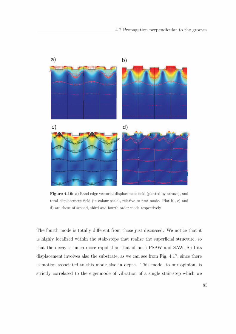
4.2 Propagation perpendicular to the grooves
a) b)
c) d)
Figure 4.16: a) Band edge vectorial displacement field (plotted by arrows), and
total displacement field (in colour scale), relative to first mode. Plot b), c) and
d) are those of second, third and fourth order mode respectively.
The fourth mode is totally different from those just discussed. We notice that it
is highly localized within the stair-steps that realize the superficial structure, so
that the decay is much more rapid than that of both PSAW and SAW. Still its
displacement involves also the substrate, as we can see from Fig. 4.17, since there
is motion associated to this mode also in depth. This mode, to our opinion, is
strictly correlated to the eigenmode of vibration of a single stair-step which we
85

4. RESULTS AND DISCUSSION
1E-7 1E-6 1E-5
1E-5
1E-4
1E-3
0.01
0.1
1
Tota
l dis
plac
emen
t (a.
u.)
Y depth (m)
Figure 4.17: Total displacement as a function of depth in the material for the
four modes present at the band edge. Red line and blue line (first and second
order mode respectively) show a SAW typical decay profile, green line (third
order mode) is the typical PSAW decayand magenta line to the fourth.
have simulated obtaining an eigenmode at about the same frequency. This single
stair-step eigenmode then slightly varies its frequency (say a part over a hundred)
and its displacement field when the simulation is realized over the entire sample
resulting as an eigenmode of the whole structure. The plot of the displacement
field along the horizontal direction (black line for the horizontal displacement, red
line for the vertical displacement and green line for the total displacement), ob-
tained as an horizontal cross section at a depth corresponding to the lower part
of the surface (Fig 4.16), shows that the first mode has the maxima of the total
displacement on the corners of the stair-steps and the minima in their center, (in
86

4.2 Propagation perpendicular to the grooves
0 5 10 15 20 25 30 35 40 45 50
X Axis ( m)
a)
Dis
plac
emen
t (a.
u.)
b)
c)
d)
Figure 4.18: Horizontal (vertical, total) displacement, at a fixed depth in the
material, as a function of the horizontal axis is plotted with black (red, green)
continuous line for each of the mode detected (a=1st mode, b=2nd mode, etc.)
fact the vertical displacement posses nodes in the central part of the stair-steps).
Conversely the second order mode has total displacement maxima in correspon-
dence of the center of the stair-steps and the minima in the cental lower part of
the superficial structure (the vertical displacement in this case posses nodes in the
center of the chosen WSC). The third mode is similar to the first in fact has its
minima at the center of the stair-steps but realizes the maximum total displace-
ment in correspondence of the central lower part (where the second mode had the
minima) instead that in the corner of the stair-steps.
87

4. RESULTS AND DISCUSSION
4.2.3 Group velocity
As it is well known the group velocity vg associated to a dispersive mode is defined,
for a generic wave vector k = (kx, ky), as
vg = (∂ω
∂kx
,∂ω
∂ky
) (4.3)
In a TG experiment the induced wave vector can be considered as one dimensional,
say k = (kx, 0), then vg = ∂ω/∂kx.
That staten it is immediately understood that the group velocity associated to
a generic mode can be obtained as the derivative of the measured dispersion curve.
However this is not a direct measurement of the group velocity. In order to realize
an accurate direct measurement of the group velocity associated to the acoustic
wavepacket it is convenient to displace the probe spot from the pump spot along
the direction where the grating is realized, so that the ratio between the relative
displacement of the two spots S and the measured arrival time t of the acoustic
wave packet is a direct measurement of the group velocity vg = S/t. We have
then slightly modified our setup. The cylindrical lens that focused the pump spot
has been removed and replaced by a simple convergent lens. To allow the relative
displacement of the two spots the mirror M in front of the exit of the probe laser,
has been mounted over a translating stage in order to realize the displacement
(along the direction where the grating is realized) between the two spots .
We have realized the measurements for different values of the experimental
wave vector (q = 0.50µm−1, q = 0.55µm−1 and q = 0.63µm−1 ' qBE) both in
the homogeneous sample and the PC. In Fig. 4.19 we show the signals obtained
on the homogeneous sample for different relative displacements of the two spots
(in black the measurement when the spots are overlapped) at the wave vector
q = 0.50µm−1: the arrival time of the wavepacket, that we define to be that cor-
88

4.2 Propagation perpendicular to the grooves
responding to the maxima of the wavepacket, increases as the distance between
the two spots is augmented as illustrated in Fig. 4.21. The same behaviour is also
present in the homogeneous sample investigated at q = 0.63µm−1.
The typical wavepacket is shown in the inset of Fig. 4.19 together with the fit
that we performed in order to determine the arrival time. The fit function that
we employed is given by the product of a gaussian distribution (the envelope of
the wavepacket) determined by the laser spot, and a sinusoidal function (oscil-
lating at the frequency of the propagative mode). The same behaviour is also
present when the homogeneous sample has been investigated at q = 0.55µm−1
and q = 0.63µm−1.
Then the PC was taken in analysis. At the wave vectors q = 0.50µm−1 and
q = 0.55µm−1 the trend is qualitatively the same observed in the homogeneous
sample: the signal is observed both when the probe and pump spots are overlapped
and when are displaced, as shown, for q = 0.50µm−1, in the upper part of Fig.4.20.
A totally different scenario is that related to the wave vector q = 0.63µm−1 ' qBE.
For this wave vector value, the signal is only obtained when the two spots are over-
lapped, while no signal is detected when the analysis is realized over the travelling
wavepacket (the two spots aren’t overlapped). This is consistent with a nearly zero
group velocity of the wavepacket. In fact the modes at the band edge are charac-
terized by a null group velocity and do not propagate, so that, when the probe is
displaced from the pump, there is no any travelling wavepacket that reaches the
probe spot to produce the signal.
The displacement S is linearly dependent on the arrival time t, the slope of the
linear fit is a direct measurement of the group velocity. In Fig. 4.21 the re-
sults obtained both for the homogeneous sample and the PC at q = 0.50µm−1,
q = 0.55µm−1 and q = 0.63µm−1 are presented.
The measured group velocities are in good agreement with those obtained from
89

4. RESULTS AND DISCUSSION
0 200 400 600 800 1000 1200
300 350 400 450 500 550
data FIT
Sig
nal a
mpl
itude
(a.u
.)
Time (ns)
Sig
nal a
mpl
itude
(a.u
.)
Time (ns)
Figure 4.19: Measured signals in the homogeneous region at q = 0.50µm−1 for
different relative displacements of the probe and the pump spot. In the inset the
typical signal associated to the travelling wavepacket is shown. The envelope of
the signal is the gaussian spot of the laser, while the fast oscillations have the
frequency of the associated mode(s).
the differentiation of the dispersion curve of the first amd second order modes of
both the homogeneous and the PC sample (see Fig. 4.22). As it can be observed
the measured values are those relative to the first mode only, since the excited
travelling wavepacket spectra contribution are dominated by the first order mode.
Using this experimental technique we clearly show a strong reduction of the group
velocity that is approaching zero when q coincide with qBE. In order to attempt a
direct measure of vg(qBE) we can follow a different approach.
As already mentioned in section 2.2 the group velocity is that responsible of the
90
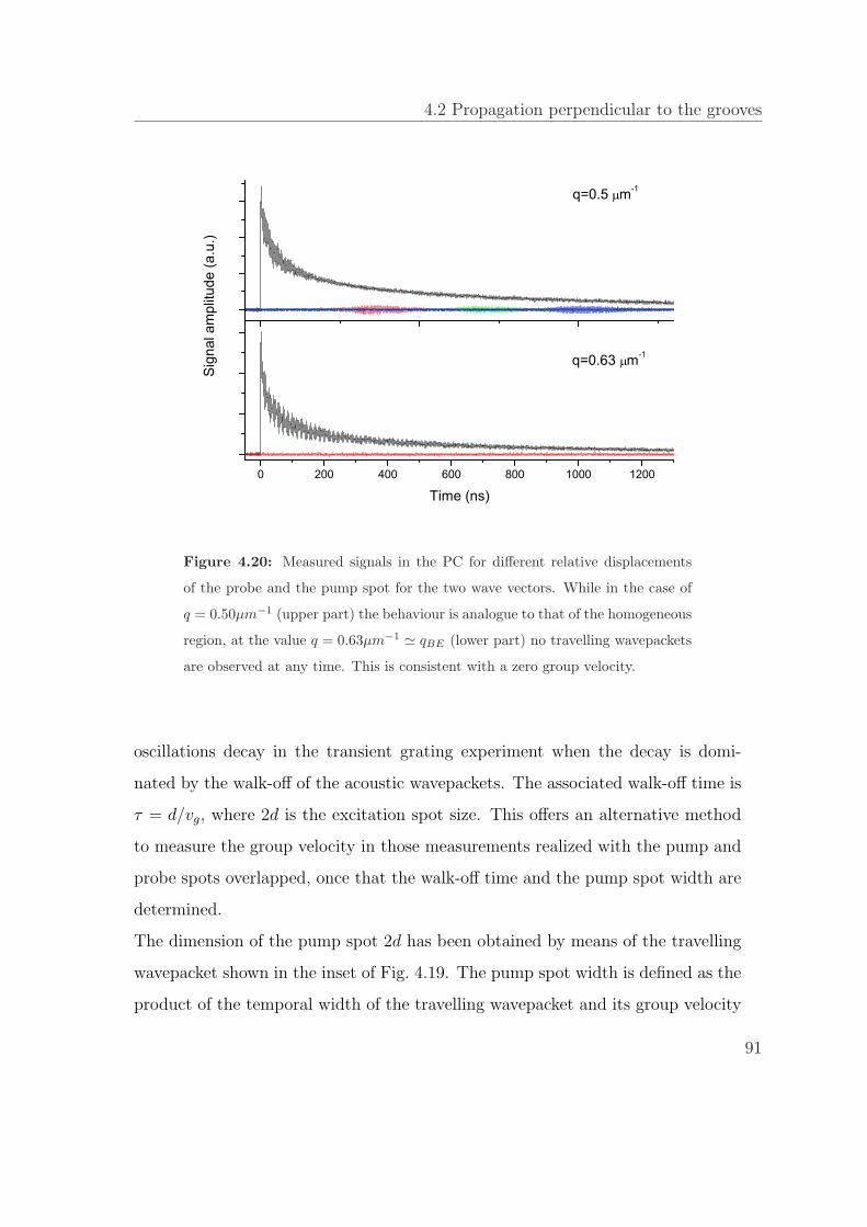
4.2 Propagation perpendicular to the grooves
0 200 400 600 800 1000 1200
Sig
nal a
mpl
itude
(a.u
.)
Time (ns)
q=0.63 m-1
q=0.5 m-1
Figure 4.20: Measured signals in the PC for different relative displacements
of the probe and the pump spot for the two wave vectors. While in the case of
q = 0.50µm−1 (upper part) the behaviour is analogue to that of the homogeneous
region, at the value q = 0.63µm−1 ' qBE (lower part) no travelling wavepackets
are observed at any time. This is consistent with a zero group velocity.
oscillations decay in the transient grating experiment when the decay is domi-
nated by the walk-off of the acoustic wavepackets. The associated walk-off time is
τ = d/vg, where 2d is the excitation spot size. This offers an alternative method
to measure the group velocity in those measurements realized with the pump and
probe spots overlapped, once that the walk-off time and the pump spot width are
determined.
The dimension of the pump spot 2d has been obtained by means of the travelling
wavepacket shown in the inset of Fig. 4.19. The pump spot width is defined as the
product of the temporal width of the travelling wavepacket and its group velocity
91
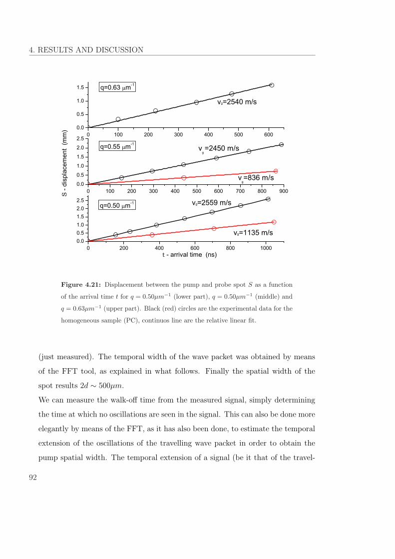
4. RESULTS AND DISCUSSION
0 200 400 600 800 10000.00.51.01.52.02.5
S -
disp
lace
men
t (m
m)
t - arrival time (ns)
vg=2559 m/s
vg=1135 m/s
q=0.50 m-1
0 100 200 300 400 500 600 700 800 9000.0
0.5
1.0
1.5
2.0
2.5q=0.55 m-1
vg
=2450 m/s
vg=836 m/s
q=0.63 m-1
vg=2540 m/s
0 100 200 300 400 500 6000.0
0.5
1.0
1.5
Figure 4.21: Displacement between the pump and probe spot S as a function
of the arrival time t for q = 0.50µm−1 (lower part), q = 0.50µm−1 (middle) and
q = 0.63µm−1 (upper part). Black (red) circles are the experimental data for the
homogeneous sample (PC), continuos line are the relative linear fit.
(just measured). The temporal width of the wave packet was obtained by means
of the FFT tool, as explained in what follows. Finally the spatial width of the
spot results 2d ∼ 500µm.
We can measure the walk-off time from the measured signal, simply determining
the time at which no oscillations are seen in the signal. This can also be done more
elegantly by means of the FFT, as it has also been done, to estimate the temporal
extension of the oscillations of the travelling wave packet in order to obtain the
pump spatial width. The temporal extension of a signal (be it that of the travel-
92

4.2 Propagation perpendicular to the grooves
0.0 0.2 0.4 0.6 0.8 1.00
1000
2000
3000
4000
5000
6000
Gro
up v
eloc
ity (m
/s)
Wave vector ( m-1)
Figure 4.22: Black full circles are the experimentally measured group velocities.
Continuous (PC) and dash-dotted (homogeneous sample) lines are the simulated
group velocities obtained as the derivative of the simulated dispersion curves
multiplied by a factor 2π. Red refers to first order modes and blue to second
order modes.
ling wavepacket, or that obtained with the pump and probe spots overlapped) is
obtained by the following procedure: subdivide the whole measured signal tempo-
ral evolution (e.g. 1µs) in time intervals of a properly chosen time window (e.g.
100ns); perform the FFT within each interval until an interval, whose FFT peak’s
magnitude is about 2% that of the peak obtained in the first interval, is found (e.g.
time interval 700−800ns). The walk-off time can be defined as that corresponding
to half of the latter interval (750ns).
In Fig. 4.23 the measurement at q ' qBE realized in the homogeneous sample
93

4. RESULTS AND DISCUSSION
0 200 400 600 800 1000 1200 1400 1600
50 100 150 200 250 300 350 400 450 500
q=0.63 m-1
Sig
nal a
mpl
itude
(a.u
.)
Time (ns)
Frequency (MHz)FF
T po
wer
(a.u
.)
Figure 4.23: Signal temporal evolution obtained at q ' qBE for the homoge-
neous sample (black) and the PC sample (red). The temporal scale over which
the signal associated to the PC sample evolves, is more than a order of magni-
tude than that of the homogeneous. In the inset the FFT power associated to
the walk-off measured time.
(black) and the PC (red) are shown. The thermal contribution to both signals has
been subtracted by means of a fit in order to clearly show and appreciate the oscil-
lating contribution. It is impressive the different timescale over which the walk-off
realizes in the two cases. This is due to the large difference between the group
velocity of the samples, in fact the excited wave vector is nearly the band edge
wave vector, that nominally implies a null group velocity for the PC. With the
estimated walk-off times we obtain a value of vg = 2490m/s for the homogeneous
sample and a extraordinary slower value for the PC vg = 180m/s. This latter value
is evidently not zero, however this can be justified in terms of the uncertainty over
94
4.3 Concluding Remark
the excited wave vector. In fact, a slight uncertainty of a ∼ 1% over the nominal
value of qBE, that we admit to have, would justify the measured group velocity.
We note that an attempt to measure slow waves by means of the walk-off time has
been realized within a recent paper [48]. However no evidence of these slow waves
was reported. In the paper the fact is attributed to an inhomogeneous broadening
arising from various factors such as scattering due to surface roughness, poly-
cristalline structure of the metal film, and the deviation of the structure from the
exact periodicity, both in the lattice step, the width and the eight of the stair-steps.
4.3 Concluding Remark
In this work we have characterized the propagation of surface acoustic waves in a
fused silica plate composed of two distinct regions: an homogeneous region and a
grooved one. The experimental characterization of the dispersion relation of the
homogeneous sample and that of the grooved sample, in the two opposite case
of wave vector parallel or orthogonal to the grooving, has been realized with a
transient grating experiment.
The characterization has been realized not only experimentally, but also theoret-
ically. The theoretical analysis has been performed with a commercial software,
that showed to be a good and reliable tool to perform band diagram character-
ization. The insight given by the simulations on the surface waves allowed to
unambiguously characterize the observed modes, both in their frequency and their
spatial form (the displacement field).
We have observed that the waves propagating in the homogeneous sample are
composed of two modes. The same holds for the waves propagating in the grooved
region with wave vector parallel to the grooves. The experimental data were in
95
4. RESULTS AND DISCUSSION
good agreement with the simulations.
When the waves are induced in the grooved sample with wave vector orthogonal
to the grooved region, the dispersion relation greatly alters from the preceding
case. Waves are affected by the periodically patterned surface and their disper-
sion relation becomes that typical of crystals: band diagram. In fact a band edge
wave vector was experimentally identified and the number of observed modes was
increased. Also in this case the agreement between the simulations and the exper-
iment was really satisfying.
Finally direct measurements of the group velocity have been performed. In these
the very first observation of really slow waves has been obtained around the band
edge wave vector.
96
Bibliography
[1] E.Yablonovitch. Phys. Rev. Lett. 58, 2059 (1987).
[2] S.John. Phys. Rev. Lett. 58, 2486 (1987).
[3] J.W.S.Rayleigh. Phyl. Mag. 26, 256 (1888).
[4] A.Khelif, A.Chouujaa, S.Benchabane, B.Djafari-Rouhani, and V.Laude. Appl.
Phys. Lett. 84, 4400 (2004).
[5] F.Cervera, L.Sanchis, J.V.Sanchez-Perez, R.Martınez-Sala, C.Rubio,
F.Meseguer, C.Lopez, D.Caballero, and J.Sanchez-Dehesa. Phys. Rev. Lett.
88, 023902 (2002).
[6] S.Zhang, L.Yin, and N.Fang. Phys. Rev. Lett. 102, 194301 (2009).
[7] S.A.Cummer and D.Schurig. New Jour. of Phys. 9, 45 (2007).
[8] M.Farhat, S.Guenneau, and S.Enoch. Phys. Rev. Lett. 103, 024301 (2009).
[9] T.Gorishnyy, C.K.Ullal, G.Fytas, and E.L.Thomas. Phys. Rev. Let. 94,
115501 (2005).
[10] B.Bonello, C.Charles, and F.Ganot. Ultasonics 44, e1259 (2006).
97
BIBLIOGRAPHY
[11] M.S.Kushwaha, P.Halevi, L.Dobrzysnki, and B.Djafari-Rouhani. Phys. Rev.
Lett. 71, 2022 (1993).
[12] M.S.Kushwaha, P.Halevi, G.Martınez, L.Dobrzynski, and B.Djafari-Rouhani.
Phys. Rev. B 49, 2313 (1994).
[13] E.N.Economu and M.M.Sigalas. Phys. Rev. B 48, 13434 (1993).
[14] M.Kafesaki, M.M.Sigalas, and E.N.Economu. Solid State Comm. 96, 285
(1995).
[15] R.Martınez-Sala, J.V.Sanchez, J., V.Gomez, J.Llinares, and Meseguer, F. Na-
ture 318, 241 (1995).
[16] J.R.Dutcher, S.Lee, B.Hillebrands, G.J.McLaughlin, B.G.Nickel, and
G.I.Stegeman. Phys. Rev. Lett. 68, 2464 (1992).
[17] S.Lee, L.Giovannini, J.R.Dutcher, F.Nizzoli, G.I.Stegeman, A.M.Marvin,
Z.Wang, J.D.Ross, A.Amoddeo, and L.S.Caputi. Phys. Rev. B 49, 2273
(1994).
[18] W.Cheng. Nature Materials 5, 830 (2006).
[19] F.R.Montero, E.Jimenez, and M.Torres. Phys. Rev. Lett. 80, 1208 (1998).
[20] D.Caballero, J.Sanchez-Dehesa, C.Rubio, R.Martinez-Sala, J.V.Sanchez-
Perez, F.Meseguer, and J.Llinares. Phys. Rev. E 60, R6316 (1999).
[21] J.O.Vasseur, P.A.Deymier, B.Chenni, B.Djafari-Rouhani, L.Dobrzynski, and
D.Prevost. Phys. Rev. Lett. 86, 3012 (2001).
[22] A.Sukhovich, L.Ling, and J.H.Page. Phys. Rev. B 77, 014301 (2008).
98
BIBLIOGRAPHY
[23] D.M.Profunnser, O.B.Wright, and O.Matsuda. Phys. Rev. Lett. 97, 055502
(2006).
[24] H.T.Grahn, H.J.Maris, and J.Tauc. IEEE J. of Quan. Ele. 25, 2562 (1989).
[25] H.N.Lin, H.J.Maris, K.Y.Lee, L., H.Luhn, and D.P.Kern. J. Appl. Phys 73,
37 (1993).
[26] G.A.Antonelli. J. Appl. Phys. 91, 3261 (2002).
[27] J.F.Robillard, A.Devos, I.Roch-Jeune, and P.A.Mante. Phys. Rev. B 78,
064302 (2008).
[28] TailphoX european project, Available at http://www.tailphox.org.
[29] L.Dhar and J.A.Rogers. Appl. Phys. Lett. 77, 1402 (2000).
[30] A.A.Maznev. Phys. Rev. B 78, 155323 (2008).
[31] L.D.Landau and E.M.Lifshitz. Course of Theoretical Physics, volume Volume
7 - Theory of Elasticity. Pergamon Press, Oxford, New York, Toronto, Sydney,
Paris, Braunschweig, (1959).
[32] J.A.Rogers, A.A.Maznev, M.J.Banet, and K.A.Nelson. Annu. Rev. Mater.
Sci. 30, 117 (2000).
[33] N.W.Ashcroft and N.D.Mermin. Solid State Physics. Saunders College,
Philadelphia, (1976).
[34] N.Bloembergen. Nonlinear optics. Benjamin, New York, (1977).
[35] Y.R.Shen. Principles of non-linear optics. John Wiley & Sons, New York,
(1984).
99

BIBLIOGRAPHY
[36] AAVV. Special issue on dynamic grating and four-wave mixing, volume 22.
IEEE J. Quant. Electron., (1986).
[37] H.J.Eichler, P.Gunter, and D.W.Pohl. Laser-Induced Dynamic Gratings.
Springer-Verlag, Berlin, (1986).
[38] Y.Yan and K.A.Nelson. J. Chem. Phys. 87, 6240 (1987).
[39] J.W.Goodman. Introduction to Fourier Optics. Mc Graw Hill, NewYork,
(1996).
[40] A.Miklos and A.Lorincz. J. Appl. Phys. 63, 2391 (1988).
[41] A.Taschin, R.Eramo, P.Bartolini, and R.Torre. Time-resolved spectroscopy of
complex liquids, chapter Transient grating experiments in glass-former liquids,
129. Springer, New York (2008).
[42] A.A.Maznev, K.A.Nelson, and J.A.Rogers. Opt. Lett. 23, 1319 (1998).
[43] G.D.Goodno, G.Dadusc, and R.J.D.Miller. J. Opt. Soc. Am. B 15, 1791
(1998).
[44] M.Terazima. J. Phys. Chem. A 103, 7401 (1999).
[45] S.Mukamel. Principles of nonlinear optical spectroscopy. Oxford University
Press, New York, (1995).
[46] N.E.Glass and A.A.Maradudin. J. Appl. Phys. 54, 796 (1983).
[47] D.Nardi, F.Banfi, C.Giannetti, B.Revaz, G.Ferrini, and F.Parmigiani. Phys.
Rev B 80, 104119 (2009).
[48] A.A.Maznev and O.B.Wright. J. Appl. Phys. 105, 123530 (2009).
100