experimental and analytical examination of golf - virginia tech
TRANSCRIPT

Experimental and Analytical Examination of GolfClub Dynamics
by
Paul R. Braunwart
Thesis submitted to the faculty of
Virginia Polytechnic Institute and State University
in partial fulfillment of the requirements for the degree of
Master of Science
in
Mechanical Engineering
Dr. Charles Knight, Chairman
Dr. Alfred Wicks
Dr. Reginald Mitchiner
December 11, 1998Blacksburg, Virginia
Keywords: Finite Element Analysis, Experimental Modal Analysis, Golf
Copyright 1998, Paul R. Braunwart

Experimental and Analytical Examination of Golf Club Dynamicsby
Paul R. BraunwartDr. Charles E. Knight, Chair
Department of Mechanical Engineering
(Abstract)
To provide the average golfer with more consistent results, manufacturers have
continued to improve the available equipment. This has led to larger club-heads, with
larger “sweet spots”, different shaft thickness for different swing styles, and the use of
advanced materials, such as graphite and titanium, for the construction.
The development of improved equipment, which utilizes advanced materials, has
spurred the need for advanced scientific analysis using a variety of techniques. Among
the most prevalent of these methods are finite element analysis and experimental modal
analysis, and use of these techniques in examining a golf club is the focus of this work.
The primary goals of this work are the development and correlation of an
appropriate finite element model, the characterization of the hands-free boundary
condition and the examination of the club golf dynamic response. To accomplish these
objectives, the physical parameters of the golf club are determined to develop the finite
element model. The analysis of natural frequencies and mode shapes correlate well with
the results extracted from experimental modal analysis for the free-free and clamped-free
boundary conditions. With the correlation established, a third boundary condition, hands-
free, is tested experimentally to ascertain the effects of the golfer’s grip on the boundary
conditions. With the FEA model confirmed, a nonlinear dynamic response of the club
during the down-swing is investigated using the nonlinear solver in Algor, and the club-
head position relative to the shaft is predicted.

iii
Acknowledgements
Dr. Charles Knight I would like to thank Dr. Knight for all of his help,
patience and guidance. Under his tutelage, I have
enhanced my knowledge of finite elements and their
applications, and I have grown in my development as
an engineer. I owe him my utmost gratitude.
Dr. Reginald Mitchiner
and Dr. Alfred Wicks
I would like to thank the members of my committee
for all their assistance and valuable advice. Their
knowledge of mechanics of materials, vibrations and
modal analysis proved to an invaluable asset.
Jim Neighbors I would like to thank Jim for all his help, especially
with the modal analysis. His assistance was
instrumental to the completion of this project, and his
patience as an office mate and friend will not be
forgotten.
Dan Clatterbuck, Steve
Weidmann and Zachary Kitts
I would like to thank these three individuals for their
entertainment, friendship and support. They have
made my time at Virginia Tech a memorable period.
Karen Kowalski I would like to thank to Karen for all her love,
patience and unwavering support. She has truly been
my guiding light.

iv
Table of Contents
Acknowledgements .................................................................................................... iiiTable of Contents ....................................................................................................... ivList of Figures ........................................................................................................... viiList of Tables ............................................................................................................. xi
Chapter 1 ..................................................................................................... 1Literature Review........................................................................................................ 3
Determination of the Club-Head Inertia Properties .................................................. 3Modal Analysis and Finite Element Analysis........................................................... 4Dynamic Response and Simulation.......................................................................... 6
Chapter 2 ..................................................................................................... 8Stiffness Matrix........................................................................................................... 9
Bar Element .......................................................................................................... 10Simple Beam ......................................................................................................... 112 Dimensional Beam Element................................................................................ 153 Dimensional Beam Element................................................................................ 16
Dynamic Analysis ..................................................................................................... 19Structural Dynamics .............................................................................................. 20
Undamped Free Vibration.................................................................................. 20Transient Response Analysis ............................................................................. 21
Formulation of the Mass and Damping Matrices........................................................ 22Mass Matrix Formulation ...................................................................................... 22Damping Matrix Formulation ................................................................................ 23
Chapter 3 ....................................................................................................26Theoretical Background ............................................................................................ 27
Single-degree of Freedom Model........................................................................... 27Multi-degree of Freedom Model ............................................................................ 29
Undamped Case................................................................................................. 30Damped Models ................................................................................................ 32
General FRF Formulation...................................................................................... 33Impulse Response.............................................................................................. 33Random Vibration ............................................................................................. 34
Modal Model Formulation......................................................................................... 35Test Configuration and Transducer Location ......................................................... 35Data Acquisition.................................................................................................... 36
Signal Analysis.................................................................................................. 37

v
H1 Estimator .................................................................................................. 38Coherence Function ....................................................................................... 38
Parameter Extraction ............................................................................................. 39SDOF Curve-fitting ........................................................................................... 39MDOF Methods ................................................................................................ 41
SDOF Extension Curve-fitting....................................................................... 41General Curve-fitting..................................................................................... 41
Modal Parameter Correlation................................................................................. 42
Chapter 4 ....................................................................................................44Coordinate System Development and Club-Head Characterization............................ 44
Lie and Loft........................................................................................................... 46Determination of the Center of Gravity...................................................................... 47Moment of Inertia...................................................................................................... 50
Moment of Inertia Setup........................................................................................ 52Setup Calibration................................................................................................... 54Determination of Club-Head Moments of Inertia ................................................... 55
Flexural Stiffness ...................................................................................................... 55Experimental Determination of EI ......................................................................... 56
Modal Analysis ......................................................................................................... 60Modal Model......................................................................................................... 61Boundary Conditions............................................................................................. 63
Free-Free Boundary Condition........................................................................... 63Clamped-Free .................................................................................................... 64Hands-Free ........................................................................................................ 65
Finite Element Analysis............................................................................................. 66Eigenvalue Analysis .............................................................................................. 66
Development of the Model ................................................................................ 67Steel Shaft.................................................................................................. 68Graphite..................................................................................................... 68
Non-Linear Dynamics ........................................................................................... 68Event Simulation ............................................................................................... 69
Chapter 5 ....................................................................................................70Club-Head Mass Moment of Inertia........................................................................... 70Shaft EI..................................................................................................................... 72Dynamic Analysis Results ......................................................................................... 82
Modal Data ........................................................................................................... 83Comparison and Correlation .................................................................................. 86
Frequency Comparison ...................................................................................... 86Steel Shaft ..................................................................................................... 86Graphite Shaft................................................................................................ 88
Mode Shape....................................................................................................... 90Steel Shaft ..................................................................................................... 91
Free-Free ................................................................................................... 91Clamped-Free ............................................................................................ 96

vi
Comparison of Hands-Free versus Free-Free and Clamped-Free .............. 101Graphite Shaft.............................................................................................. 105
Free-Free ................................................................................................. 106Clamped-Free .......................................................................................... 107Comparison of Hands-Free versus Free-Free and Clamped-Free .............. 108
Nonlinear Dynamic Analysis ............................................................................... 109Determination of Moment Curve ..................................................................... 110Dynamic Response .......................................................................................... 112
Summary of Results and Conclusions...................................................................... 113Summary of Results ............................................................................................ 114
Future Work............................................................................................................ 116
References ................................................................................................118
Appendix A - Graphite Shaft Results .........................................................121Free-Free Boundary Conditions........................................................................... 121
Droop Plane..................................................................................................... 121Swing Plane..................................................................................................... 122
Clamped-Free...................................................................................................... 124Droop-Plane .................................................................................................... 124Swing-Plane .................................................................................................... 125
Comparison of Hands-Free versus Free-Free and Clamped-Free.......................... 127Hands-Free vs. Free-Free................................................................................. 127Hands-Free vs. Clamped-Free.......................................................................... 128
Appendix B – Computer Programs............................................................130Freqtest.m ........................................................................................................... 130
Vita ......................................................................................................................... 133

vii
List of Figures
Figure 2.1 Nodal Forces associated with deformation of a two-node barelement. (a) Node 1 displaced u1 units. (b) Node 2 displacedu2 units. (From Reference 24)..................................................................... 10
Figure 2.2 (a) Simple plane beam element and its nodal d.o.f. (b) Nodalloads associated with the d.o.f. (From Reference 24)................................. 11
Figure 2.3 (a-d) Deflected shapes associated with activation of eachd.o.f. in turn. (From Reference 24) ............................................................ 12
Figure 2.4 3-D beam element oriented with respect to local and globalcoordinate systems. .................................................................................... 16
Figure 2.5 3-D beam element nodal degrees of freedom expressed in (a)local coordinates and (b) global coordinates. (FromReference 24)............................................................................................. 17
Figure 3.1 Linear model with noise m(t) and n(t) at input and output .......................... 37
Figure 3.2 Half-power points and natural frequency for the PeakAmplitude Method (From Reference 28)................................................... 40
Figure 4.1 Measured Points using a three axis mill and dial indicator.......................... 45
Figure 4.2 Club-head Lie and Loft (a) Lie Angle. (b) Loft Angle .............................. 46
Figure 4.3 Determination of x and z coordinates of c.g. .............................................. 48
Figure 4.4 Determination of the y-position of the Centroid.......................................... 49
Figure 4.5 Experimental Setup for the Determination of Club-Head MassMoment of Inertia ...................................................................................... 51
Figure 4.6 Setup Components ..................................................................................... 53
Figure 4.7 Test Specimen Used for Calibration ........................................................... 54
Figure 4.8 (a) 90 Degree Connector (b) 45 Degree Connector................................... 55

viii
Figure 4.9 (a) Concentrated Load Applied by Instron Tester. (b)Corresponding Theoretical Representation of Applied Loadand Supports .............................................................................................. 57
Figure 4.10 The Ovalization of the Shaft Due to Localized Deflection byConcentrated Load..................................................................................... 58
Figure 4.11 (a) Distributed Load Applied by Instron Tester. (b)Corresponding Theoretical Representation of Applied Loadand Supports .............................................................................................. 59
Figure 4.12 Modal Setup for the Free-Free Boundary Conditions.................................. 64
Figure 4.13 Modal Setup for the Clamped-Free............................................................. 65
Figure 4.14 Modal Setup for Hands-Free ...................................................................... 66
Figure 5.1 (a) Determination of k Using a Linear Least SquaresTechnique (b) Curve-Fit Residuals ........................................................... 73
Figure 5.2 Comparison of Theoretical and Experimental Techniques forthe Determination of the Moment of Inertia for an 8 inchBeam with a Mid-Span Load and Simple Supports..................................... 74
Figure 5.3 Exaggerated Ovalization of the Shaft at the Point of LoadApplication. ............................................................................................... 75
Figure 5.4 Comparison of Deflection Values for Finite Element,Experimental, and Theoretical Methods ..................................................... 76
Figure 5.5 Comparison of the percent discrepancies of 8 and 12 inchsimply-supported span with a 25 lb load applied mid-span. ........................ 77
Figure 5.6 Comparison of the percent discrepancies of a 12 inch under adistributed load with simply supported and distributedsupports. .................................................................................................... 78
Figure 5.7 Comparison of experimental and theoretical deflections forsteel shaft................................................................................................... 79
Figure 5.8 Comparison of experimental and theoretical moments ofinertia......................................................................................................... 79
Figure 5.9 Comparison of the EI curves for the steel and graphite shafts. .................... 80

ix
Figure 5.10 (a) Fifth order least-squares curve-fit of the experimentalmoment of inertia data for the 75H graphite shaft. (b)Corresponding curve-fit residuals............................................................... 81
Figure 5.11 Steel shaft, free-free driving point FRF. (a) Amplitude (b)Coherence.................................................................................................. 84
Figure 5.12 Comparison of driving point FRFs for steel shaft – 2nd swingplane mode. (a) Amplitude (b) Phase...................................................... 85
Figure 5.13 Comparison of the mass-normalized mode shapes for thedroop-plane of the steel shaft with free-free boundaryconditions. (a) First Mode (b) Second Mode (c) ThirdMode ......................................................................................................... 93
Figure 5.14 Comparison of the mass-normalized mode shapes for theswing-plane of the steel shaft with free-free boundaryconditions. (a) First Mode (b) Second Mode (c) ThirdMode ......................................................................................................... 94
Figure 5.15 Comparison of the mass-normalized mode shapes for thedroop-plane of the steel shaft with clamped-free boundaryconditions. (a) First Mode (b) Second Mode (c) ThirdMode ......................................................................................................... 97
Figure 5.16 Comparison of the mass-normalized mode shapes for thedroop-plane of the steel shaft with clamped-free boundaryconditions. (a) First Mode (b) Second Mode (c) ThirdMode ......................................................................................................... 98
Figure 5.17 Comparison of first and second droop modes for the steelshaft......................................................................................................... 101
Figure 5.18 Comparison of the mass-normalized mode shapes for theswing-plane of the steel shaft with free-free versus hands-freeboundary conditions. (a) First Mode (b) Second Mode (c)Third Mode.............................................................................................. 102
Figure 5.19 Comparison of the mass-normalized mode shapes for theswing-plane of the steel shaft with clamped-free versus hands-free boundary conditions. (a) First Mode (b) Second Mode(c) Third Mode........................................................................................ 104
Figure 5.20 Calibration of strain gauges for two steel shafts........................................ 110
Figure 5.21 Moment for curve for the swing-plane...................................................... 111

x
Figure 5.22 Development of Accupak event curve using consecutivelinear approximations............................................................................... 112
Figure 5.23 Dynamic swing results obtained using Accupak softwareutility in Algor. ........................................................................................ 113
Figure A.1 Comparison of the mass-normalized mode shapes for thedroop-plane of the graphite shaft with free-free boundaryconditions. (a) First Mode (b) Second Mode (c) ThirdMode ....................................................................................................... 122
Figure A.2 Comparison of the mass-normalized mode shapes for theswing-plane of the graphite shaft with free-free boundaryconditions. (a) First Mode (b) Second Mode (c) ThirdMode ....................................................................................................... 123
Figure A.3 Comparison of the mass-normalized mode shapes for thedroop-plane of the graphite shaft with clamped-free boundaryconditions. (a) First Mode (b) Second Mode (c) ThirdMode ....................................................................................................... 125
Figure A.4 Comparison of the mass-normalized mode shapes for theswing-plane of the graphite shaft with clamped-free boundaryconditions. (a) First Mode (b) Second Mode (c) ThirdMode ....................................................................................................... 126
Figure A.5 Comparison of the mass-normalized mode shapes for theswing-plane of the graphite shaft with free-free versus hands-free boundary conditions. (a) First Mode (b) Second Mode(c) Third Mode........................................................................................ 128
Figure A.6 Comparison of the mass-normalized mode shapes for theswing-plane of the graphite shaft with clamped-free versushands-free boundary conditions. (a) First Mode (b) SecondMode (c) Third Mode............................................................................. 129

xi
List of Tables
Table 4.1 Coordinates for the Club-Head in the Desired System ................................ 46
Table 4.2 Summary of modal test settings.................................................................. 62
Table 5.1 Mode frequencies for steel shaft. (a) Free-Free (b)Clamped-Free 87
Table 5.2 Mode frequencies for the hands-free boundary condition forthe steel shaft. ............................................................................................ 87
Table 5.3 Mode frequency comparison between hands-free and the free-free and clamped-free cases........................................................................ 88
Table 5.4 Mode frequencies for graphite shaft. (a) Free-Free (b)Clamped-Free ............................................................................................ 89
Table 5.5 Mode frequencies for the hands-free boundary condition forthe steel shaft. ............................................................................................ 90
Table 5.6 Mode frequency comparison between hands-free and the free-free and clamped-free cases........................................................................ 90
Table 5.7 Free-Free MAC for steel shaft (a) Droop-plane (b) SwingPlane.......................................................................................................... 96
Table 5.8 Clamped-Free MAC for steel shaft (a) Droop-plane (b)Swing Plane ............................................................................................. 100
Table 5.9 Free-free versus hand-free MAC for steel shaft ........................................ 105
Table 5.10 Free-Free MAC for graphite shaft. (a) Droop Plane (b)Swing Plane ............................................................................................. 107
Table 5.11 Clamped-Free MAC for graphite shaft. (a) Droop Plane (b)Swing Plane ............................................................................................. 108
Table 5.12 Free-free versus hand-free MAC for graphite shaft................................... 109

1
Chapter 1
Introduction and Literature Review
The game of golf is an enigma. Shots, which are solidly hit straight and true on
one day, may slice, fade or hook on the next, and for years, golfers of all ages have
attempted to conquer, or at least understand, the mysterious nature of this game. To
provide the average player with more consistent results, manufacturers have continued to
improve the available equipment. This has led to larger club-heads, with larger
corresponding “sweet spots”, different shaft thickness for different swing styles, and the
use of advanced materials, such as graphite and titanium, for the construction.
The development of improved equipment, which utilizes advanced materials, has
spurred the need for advanced scientific analysis using a variety of techniques. Among
the most prevalent of these methods are finite element analysis and experimental modal
analysis, and use of these techniques in examining a golf club is the focus of this
research.
The finite element method is a numerical method for analyzing structures and
system that are typically too complex to be analyzed through standard analytical

2
techniques. In this technique, a structure is divided piecewise into elements, and the
performance of each element is then simply characterized. The elements are then
connected, and the resulting algebraic equations are simultaneously solved utilizing
computational capabilities.
Experimental modal analysis has emerged as an extremely useful procedure.
Performed under controlled conditions, it encompasses excitation of a structure, or
component; acquisition of data; and the subsequent analysis of the response. The uses of
modal analysis are varied and range from determination of natural frequencies and
damping factor to full development of a mass-spring-damper model of a particular
system.
For this work, a finite element model, which uses beam elements, is developed
from analytically and experimentally determined data and is used to examine the dynamic
response of the golf club. The number of elements is increased until convergence, and
resulting eigenvalues and eigenvectors are subsequently correlated with results from
experimental modal analysis.
Two boundary conditions, free-free and clamped-free, are employed for both
techniques since these conditions are among easiest and most widely used for both
methods. Also, an additional case, hands-free, is investigated solely using modal analysis
to ascertain the boundary conditions of a typical grip.
The experimental modal analysis is performed on a golf club, and the mode
frequencies and mode shapes are then extracted for three different boundary conditions.
The first two boundary conditions, free-free and clamped-free, are used to compare with
3
the finite element model, while the final case, hands-free, is employed to simulate the
conditions due the golfer gripping the club.
The finite element analysis (FEA) and experimental modal analysis (EMA) results
are correlated to determine the suitability of the finite element model, and with this
established, the nonlinear dynamic response of the club during the down-swing is
investigated using FEA in the software package Algor®. To accomplish this task, swing
shaft strain data is first calibrated and converted to produce an input moment curve,
which is then approximated in the software. This information is input into the software,
which automatically converges the model at the desired time steps, and the results are
then examined to determine shaft and club-head response, with special interest in the
club-head position at impact with the ball.
Literature Review
The earliest scientific analysis of the golf-swing and club performance is
contained in Cochran and Stobbs’ [1] groundbreaking work, The Search for the Perfect
Swing. Since its publication in 1968, numerous scientific articles concerning golf have
been published, and three scientific congresses on the game have been held.
Determination of the Club-Head Inertia Properties
The center of gravity of a structure is traditionally determined by suspending an
object at several different points, noting the position and using the principles of statics.
To determine the club-head center of gravity, Thomas, Deiter and Best [2] utilize a similar
technique. The club-head is suspended from a string and photographed with the
appropriate scale, and the center of gravity is then determined from the scales and

4
photographs. This method can be quite cumbersome, so Twigg and Butler [3] utilize an
“analytical balance” with a sliding beam balance and the sum of moments principle about
a pivot to determine the center of gravity.
The club-head moments of inertia are generally determined using two different
approaches. The first method, utilized by Thomas et al [2] and Johnson [4], uses a
pendulum to determine the moment of inertia about three axes. The values are obtained
for a second coordinate system, and the principle moments of inertia are then determined
using the direction cosines between the two coordinate systems or by solving the inertia
matrix. For the other method, used by Twigg and Butler, the moment of inertia is
obtained by spinning the object on a spring attached to a drill motor, and “as the system
reaches steady-state”, the object will align itself with a principle moment axis.
Modal Analysis and Finite Element Analysis
The use of modal analysis and finite element analysis has increased in the
determination of shaft response. The correlation of FEA and EMA is examined in a
number of articles, with most focusing on the correlation of results for particular
boundary conditions and some attempting to characterize the hands-free case as either
free-free or clamped-free.
In their work, Swider and Ferraris [5] model the shaft and club-head using plate
elements but consider only a clamped-free boundary condition for the club. Examination
of the results reveals “good” correlation between the experimental and finite element
mode shapes and frequencies, and this suggests that an appropriate FEA model can be
developed for the club.

5
Okubo and Simada [6] consider the three boundary conditions – free-free,
clamped-free and hands. In this case, tests are performed solely on 1 wood, and the EMA
results are compared with “the vibration and strain mode shapes generated using
computer aided engineering.” Based upon their results, the authors suggest that the
boundary conditions due to gripping vary through the swing, with the conditions similar
to clamped-free at lower frequencies and closer to the free-free case at higher
frequencies.
Thomas, Deiter and Best [2] model the shaft using tapered beam elements, and the
club-head is modeled as a lumped mass at the center of gravity. Three boundary
conditions are again employed, but for the finite element analysis, the hands-free case is
assumed to be a clamped-free case using springs to represent the hands. Additionally,
only the FEA and EMA frequency results are compared, with no comparison of mode
shapes included.
Friswell, Smart and Mottershead [7] also utilize beam elements, but only the
clamped-free boundary condition is analyzed to avoid any uncertainty that may be
associated with the hands-free boundary condition. The club-head mass moments of
inertia are initially determined from a computer-aided design (CAD) package and then
updated in their model.
Experimental frequencies are determined directly from the frequency response
functions (FRFs) and then compared with the initial and updated FEA results. Friswell,
Smart and Mottershead suggest that mode shapes are difficult to obtain “due the mass
loading of the accelerometer”, and thus the typical “modal analysis techniques, using a
roving accelerometer or roving hammer excitation, are impractical on the golf club.”

6
Dynamic Response and Simulation
Cochran and Stobbs provide the earliest analysis of the golf swing and the shaft
response. In the work, Cochran and Stobbs model the golfer and the golf club as a two-
pendulum system, with the upper pendulum constituting the golfer’s shoulders and arms.
With the wrists as a pivot, the lower pendulum consists of the club, hands and wrist.
Using this double pendulum model, Budney and Bellows [8] develop a dynamic
model of the club to relate the forces and torques that are present during the swing.
Expanding on this, a kinetic analysis of the golf swing is performed, which establishes
the force curve for the swing. [9]
While the double pendulum model is the most commonly held, the swing can also
be modeled as a cantilever beam that is attached to a rotating hub. Using this method, the
natural frequencies have been determined by Schilansl [10], Rao and Carnegie [11] and
Pnuelli [12].
The dynamic deflections are determined by both Christensen and Lee [13] and
Yoo, Ryan and Scott [14]. Christensen and Lee utilize a Newton-Raphson method to solve
a nonlinear finite element model, which considers both axial and transverse deflections.
Meanwhile, Yoo, Ryan and Scott use the Raleigh-Ritz method to solve a set of linearized
equations, which account for the both axial and transverse deflections.
The effects of tip mass are introduced in the works of Bhat [15], Hoa [16], Lee [17],
Putter and Mannor [18] and Winfield and Soriano [19]. In Bhat’s approach, the mode
frequencies and mode shapes are determined by the Raleigh-Ritz method, while the
remaining approaches use the finite element method to determine the natural frequencies.

7
In their work, Winfield and Soriano determine “the dynamic response of the beam
due to a specified hub rotation”, and the results of this analysis suggest that the club-head
“kicks” or “springs back” just before impact with the ball. In other words, the club-head
position is behind the shaft through the majority of the swing, but just prior to impact, the
club-head quickly moves to a position just in front of the shaft. This sudden change of
club-head position, or “kick”, is then thought to impart greater momentum on the ball.
This “kick” phenomenon has also been the focus of other works, and there
appears to be a slight controversy on the actual club-head position just prior to impact.
On one side, Horwood [20]. Thomas et al [2], Masuda and Korjima [21] all believe that the
club-head “springs back” just beforehand. On the other side, Milne [22] and Milne and
Davis [23] believe the club-head lags just before impact.
8
Chapter 2
Finite Element Theory
The finite element method is a numerical method for analyzing structures which
are usually too complicated to be solved through standard analytical techniques. In this
method, a structure is divided piecewise into elements, and the response of each element
is simply characterized. The elements are connected, and the resulting algebraic
equations are simultaneously solved utilizing computational capabilities.
The finite element method is utilized in a wide range of applications including,
heat transfer, fluid mechanics, acoustics, electromagnetism, and structural mechanics, and
the desired field quantity is particular to each area of interest. The primary interest of this
work is the area of structural dynamics, and the desired field quantities are the natural
frequencies and displacement response.
A brief discussion of the element formulation and solution techniques is discussed
in the subsequent sections. The formulation of the stiffness matrix for beam elements is
first considered, and the various types of dynamic analysis and the formulations of the
mass and damping matrices follow.

9
Stiffness Matrix
The stiffness matrix relates nodal displacements to nodal forces. There are three
basic methods used to determine the stiffness matrix – the direct method, the variational
method, and the weighted residual method.
The direct method, based on physical understanding, is limited to simple
elements, but is helpful in understanding the finite element method. In this technique,
force components and general displacements are related by the following equation,
fkd = (2.1)
k is the element stiffness matrix, d is the associated nodal displacement vector, and f is
the internal force component vector. Considering the physical characteristics of the
element, the stiffness matrix is produced from the superposition of simple element
solutions. Applying a unit displacement to one component while the remaining
components remain zero, the magnitude of the force required to maintain the
displacement state is evaluated. The procedure is repeated for the remaining components,
and the values are recorded in matrix form.
The development of the stiffness matrix is first examined for a bar element and
the simple beam element. Using superposition, the2-D plane beam and 3-D beam
element are developed from these two elements and basic beam theory.
10
Bar Element
Lx
u1
F11 F21
1
F11= F21
A,E
2
(a)
Lx
u2
F12 F22
1
F12= F22
A,E
2
(b)
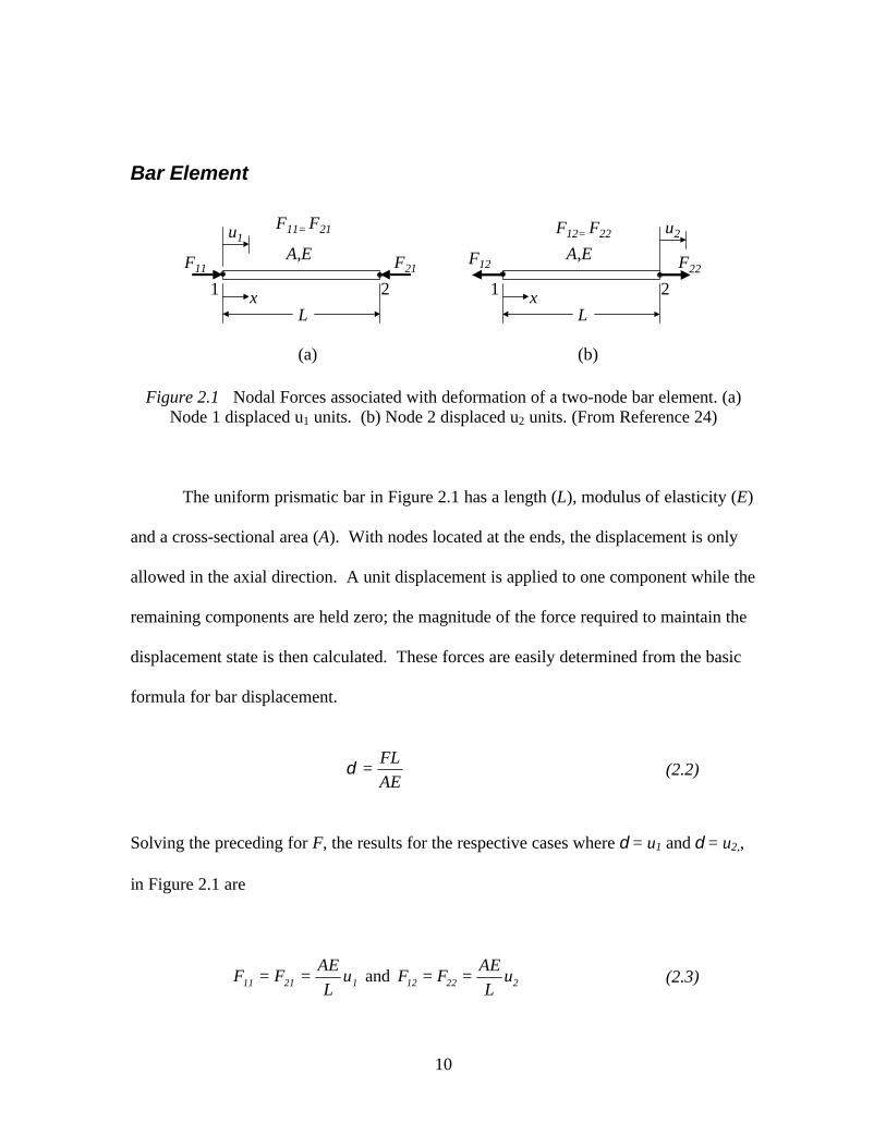
Figure 2.1 Nodal Forces associated with deformation of a two-node bar element. (a)Node 1 displaced u1 units. (b) Node 2 displaced u2 units. (From Reference 24)
The uniform prismatic bar in Figure 2.1 has a length (L), modulus of elasticity (E)
and a cross-sectional area (A). With nodes located at the ends, the displacement is only
allowed in the axial direction. A unit displacement is applied to one component while the
remaining components are held zero; the magnitude of the force required to maintain the
displacement state is then calculated. These forces are easily determined from the basic
formula for bar displacement.
AEFL
=δ (2.2)
Solving the preceding for F, the results for the respective cases where δ = u1 and δ = u2,,
in Figure 2.1 are
12111 uL
AEFF == and 22212 u
LAE
FF == (2.3)

11
Fij is the force at node i associated with the node j displacement, and these results can
then be written in matrix form. Using the sign convention that force and displacements
are positive to the right, the matrix form is thus,
=
−
−
2
1
2221
1211
F
F
1
1
FF
FF or
=
−
−
2
1
2
1
F
F
u
u
11
11
LAE
(2.4)
Here, F1 and F2 are the resultant, internal forces applied to the bar at nodes 1 and 2
respectively.
Simple Beam
With the bar element completed, a simple beam element is considered. It is
prismatic with a modulus of elasticity, E, and a centroidal area moment of inertia, I, of its
cross-sectional area. From Euler beam theory, the centerline, lateral displacement,
v=v(x), is a cubic polynomial in x for a uniform prismatic beam with loads only at the
ends. (Figure 2.2) The associated degrees of freedom are two lateral translations, v1 and
v2, and two rotations parallel to the z-axis, θz1 and θz2.
Lv1 v2
θz1 θz2 x
y,v
E, I
(a)
LF1 F2
M1 M2 xE, I
y,v
(b)
Figure 2.2 (a) Simple plane beam element and its nodal d.o.f. (b) Nodal loadsassociated with the d.o.f. (From Reference 24)

12
Using a similar procedure to the bar element, the stiffness matrix for the simple
beam element can be constructed column by column using the principles of beam theory
and superposition. As before, a unit displacement is applied to one component while the
remaining components remain zero, and the magnitude of the force and moments
required to maintain the displacement state must then be evaluated.
LF1
F2
M1
M2v1 = 1
LF1 F2
M1M2θz1 = 1
(a) (b)
LF1
F2
M1
M2
v2 = 1
L
F1 F2
M1 M2
θz2 = 1
(c) (d)
Figure 2.3 (a-d) Deflected shapes associated with activation of each d.o.f. in turn.(From Reference 24)
As an example, the development of the first column of the stiffness matrix is
considered. Using the element in Figure 2.2, a unit vertical displacement, v1 = 1, is
applied with the remaining values (v2, θz1 and θz2) held to zero, and the depicted
deflection of Figure 2.3a results. To produce this deflection, the appropriate nodal forces
and moments are superposed, and the element equations expressed in matrix form are,

13
=
2
2
1
1
44434241
34333231
24232221
14131211
M
F
M
F
0
0
0
1
kkkk
kkkk
kkkk
kkkk
(2.5)
From the preceding, the following relationships can be defined,
111 Fk =
121 Mk =
231 Fk =
241 Mk =
(2.6)
These nodal forces and moments are then related to deflection and rotation using
superposition and beam equations,
EI2
LM
EI3
LF1v
21
31
1 −==
EI
LM
EI2
LF0 1
21
1z −==θ
(2.7)
Solving the preceding simultaneously yields,
31 LEI12
F =
21 LEI6
M =
(2.8)
The values for the F2 and M2 are then determined using the principles of statics,

14
32 LEI12
F −=
22 LEI6
M =
(2.9)
Using the relationships in equation (2.6), the values for the first column of the stiffness
matrix are thus determined.
Using similar procedures, the remaining columns are determined, and the
resulting stiffness matrix, k, is
−
−−−
−
−
=
LEI4
LEI6
LEI2
LEI6
LEI6
LEI12
LEI6
LEI12
LEI2
L
EI6LEI4
L
EI6
L
EI6
L
EI12
L
EI6
L
EI12
22
2323
22
2323
k (2.10)
This is the stiffness matrix associated with [ ]T2z21z1 vv θθ=d , and this formulation
provides an exact representation of the beam using traditional beam theory for loads
applied at the nodes. For load distributed across the span, the solution is inexact but
approaches the exact solution with increased numbers of element. Therefore, careful
modeling should be employed when using this formulation.

15
2 Dimensional Beam Element
While the foregoing formulation is useful for simple beams, another formulation
is desired when axial loads exist as well. The 2-D beam element, also called a plane
frame element, considers axial loads, shear force and rotation in one direction, and it is
formed by the superposition of the simple bar element and the simple beam. Combining
equations (2.4) and (2.10), the resulting stiffness matrix along the x-axis is
−
−−−
−
−
−
−
=
LEI4
LEI6
0LEI2
LEI6
0
L
EI6
L
EI120
L
EI6
L
EI120
00L
AE00
LAE
LEI2
L
EI60
LEI4
L
EI60
L
EI6
L
EI120
L
EI6
L
EI120
00L
AE00
LAE
22
2323
22
2323
k (2.11)
The matrix superposes the stiffness matrices of the bar and beam, and hence, the d.o.f
vector is [ ]T2z121z11 vuvu θθ=d .
As with all element formulations, care must taken when employing this element.
For small displacements, this superposition of elements “will be accurate, however there
is an interaction that occurs between axial and lateral loading on beams.” [25] The effects
of a tensile axial load tend to attenuate the effect of lateral loads. Conversely, a
compressive axial load tends to magnify the effect of the later loads.

16
3 Dimensional Beam Element
The beam element most often utilized in general finite element codes has 3-
dimensional capability and is also termed a “space beam” element. To develop this
element, the formulation must include “the capability for torsional loads about the axis of
the line element as well as flexural loads acting in the x-z plan” [25] First, a local
coordinate system, xyz, is established for a beam element in the global, XYZ coordinate
system. (See Figure 2.4) The x-axis is along the line of the element, the y-axis is one
lateral direction, and the z-axis, along the orthogonal lateral direction, completes the
right-hand coordinate system.
xy
z X
Z
Y
2
1
Figure 2.4 3-D beam element oriented with respect to local and global coordinatesystems.

17
Using the relationship of torque and angle of twist from basic mechanics of
materials, the effects of torsion are added through superposition. For a two-node
element, the relationship is given by following equation in matrix notation.
=
−
−
j
i
xj
xi
T
T
LJG
LJG
LJG
LJG
φ
φ (2.12)
J is a torsional constant about the x-axis, but for a beam with circular cross-section, it is
the polar moment of inertia. G is the modulus of rigidity, L is the element length, and φxi
and φxj are the nodal d.o.f. associated with the angle of twist at each node about the x-
axis. Finally, Ti and Tj are the torques or moments about the x-axis for the individual
nodes.
uXi
vi
wi
θxi
θyi
θzi
θXi
vYi
wZi
θYi
θZi
(a) (b)
Figure 2.5 3-D beam element nodal degrees of freedom expressed in (a) localcoordinates and (b) global coordinates. (From Reference 24)

18
With the addition of flexure in the x-z plane, another stiffness matrix, similar to
the one in equation (2.11), is added. In this case, the area moment of inertia is about the
y-axis and passes through the cross-sectional, neutral axis.
These two matrices are then superimposed with the stiffness matrix from equation
(2.13), and this yields the 12 x 12 stiffness matrix in equation.
−
−
−−
−
−−−
−
−
−
−
−−−
−
−
L
EI4000
L
EI60
L
EI2000
L
EI60
0L
EI40
L
EI6000
L
EI20
L
EI600
00L
JG00000
LJG
000
0L
EI60
L
EI12000
L
EI60
L
EI1200
L
EI6000
L
EI120
L
EI6000
L
EI120
00000L
AE00000
LAE
L
EI2000
L
EI60
L
EI4000
L
EI60
0L
EI20
L
EI6000
L
EI40
L
EI600
00L
JG00000
LJG
000
0L
EI60
L
EI12000
L
EI60
L
EI1200
L
EI6000
L
EI120
L
EI6000
L
EI120
00000LAE
00000L
AE
z2
zx2
z
y
2
yy
2
y
2
y
3
y
2
y
3
y
2z
3z
3z
3z
z2
zz2
z
y
2
yy
2
y
2
y
3
y
2
y
3
y
2z
3z
2z
3z
(2.13)
This is the stiffness matrix in the local coordinate system in Figure 2.4,
and its corresponding displacement vector,
{ }T2z2y2x2221z1y1x111 wvuwvud θθθθθθ= . To formulate this matrix
for the global coordinate system, a coordinate transformation must be performed.

19
Since this element is based upon conventional beam theory, this element is
limited by the fundamental assumptions of conventional beam and torsion theories, and
the results can only be as accurate as the theory. Also, this formulation fails to couple the
lateral and axial loading, and nonlinear coupling does exist between the two. The
analysis also does not account for stress concentration factors at changes in cross-section
nor point load applications.
Dynamic Analysis
To account for inertial effects, dynamic analysis utilizes mass and damping
matrices as well as the stiffness matrix. For a structure modeled by a finite number of
nodal d.o.f., the set differential equations of motion for dynamic analysis can be in
expressed in matrix form.
FKDDCDM =++ &&& (2.14)
Here, M is mass matrix of the structure, D&& is the nodal acceleration vector, C is the
damping matrix of the structure, and D& is the nodal velocity vector. K is again the
stiffness matrix of the structure, D is the nodal displacement vector, and F is the time-
variable nodal load vector.
Equation (2.14) is the general equation for all dynamic problems, but these
problems can be classified as either wave propagation or structural dynamics. Wave
propagation problems typically have impact or blast loading. The response is generally
replete with high frequencies, and effects of stress waves are the primary interest. In
structural dynamics, the frequency of excitation is generally in the same range as the

20
lowest natural frequencies of the structure. Structural dynamics is usually subdivided
into eigenvalue analysis and time-history analysis. In eigenvalue analysis, the natural
frequency and the corresponding mode shapes of a structure are desired, while in time-
history analysis, the movements of the structure under prescribed conditions are sought.
This category includes frequency response analysis and transient response analysis. In
frequency response analysis, the steady state response of the structure to harmonic force
input is also harmonic; while the loading is an arbitrary time dependent function for
transient response analysis.
Structural Dynamics
For this work, the natural frequencies, mode shapes and response under
designated conditions are the primary interests. Therefore, the two structural dynamics
subdivisions will be briefly examined here, while a thorough discussion of wave
propagation problems, or shock loading problems is included in references [24] and [26].
Undamped Free Vibration
In structural dynamics analysis, the eigenvalue analysis is the most typical form.
Here, the undamped free vibration of a system by an initial disturbance is the focus, and
the natural frequencies and corresponding mode shapes are primarily sought. To
accomplish this, the applied forces, F, and damping matrix, C, in equation (2.14) are set
to zero. The motion of each node is then assumed to be a “sinusoidal function of the
peak displacement amplitude for that node” [25], and the displacement vector is also
sinusoidal. The system can then be expressed as,
( ) 0AMK =− 2ω (2.15)

21
ω2 is the eigenvalue, and for the trivial case, equation (2.15) has the solution D = 0. The
nontrivial solutions are the primary interest and are the same number as the nodal degrees
of freedom.
For a nontrivial case, the determinant of the ( )MK 2ω− matrix must be zero, and
solution yields the characteristic equation where the roots are the eigenvalues - ω2. The
natural frequencies are then calculated, and the corresponding eigenvector - φφ, a set of
relative node displacements, can be determined. This is accomplished by substitution of
ω2 into equation (2.15) and solving for A. A is then normalized, and the result is the
eigenvector, or normal mode shape, for a particular eigenvalue.
Although the solution of the eigenproblem yields a natural frequency for each
d.o.f., the nature of the finite element approximation yields high inaccuracies in the
higher eigenvalues and eigenvectors. Only the lowest eigenvalues of a model are
generally considered because the primary response typically involves only the lowest
natural frequencies.
Transient Response Analysis
Transient response analysis is performed when arbitrary time-dependent loading
function is used rather than a harmonic load. Two general approaches, direct integration
and modal superposition, are used to solve this type of problem. In the direct integration,
the system equations are first analyzed using finite elements and subsequently integrated
in the time for the velocity and acceleration component. While the preceding technique
requires considerable computing resources, the modal superposition technique alleviates
some of the burden. The approach assumes that the superposition of lower frequency

22
mode shapes sufficiently represents the actual dynamic response of the system.
Basically, the node displacement coordinates are changed to a set of modal coordinates;
therefore, the set of system equations is reduced from one per nodal d.o.f. to a set of
modal equations for the desired number of modes. Several solution algorithms have been
developed for the two techniques, and a few are discussed in reference [26].
Formulation of the Mass and Damping Matrices
For the various dynamic analysis techniques examined previously, the solution
includes the mass and damping matrices, but the formation of each has yet to be
discussed. Analogous to the formulation of the stiffness matrix, the matrices are first
formulated on the elemental level, the structural level matrices are then developed.
Mass Matrix Formulation
The formulation of the mass matrix begins by employing D’Alembert principle to
develop body forces and then uses a work equivalent distribution. The general form of
mass matrix, m, is thus,
∫= dVT ρNNm (2.16)
N is the element shape function matrix, ρ is the mass density, and dV is the incremental
volume. Since this mass matrix uses the same shape functions as the stiffness matrix, it is
commonly called the “consistent” mass matrix. When applied to the bar element (Figure
2.1), the matrix is
23
=
3AL
6AL
6AL
3AL
ρρ
ρρ
m (2.17)
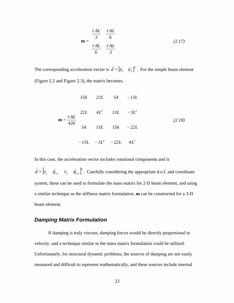
The corresponding acceleration vector is [ ]T21 uud &&&&&& = . For the simple beam element
(Figure 2.2 and Figure 2.3), the matrix becomes.
−−−
−
−
−
=
22
22
L4L22L3L13
L22156L1354
L3L13L4L22
L1354L22156
420ALρ
m (2.18)
In this case, the acceleration vector includes rotational components and is
[ ]T2z21z1 vvd θθ &&&&&&&&&& = . Carefully considering the appropriate d.o.f. and coordinate
system, these can be used to formulate the mass matrix for 2-D beam element, and using
a similar technique as the stiffness matrix formulation, m can be constructed for a 3-D
beam element.
Damping Matrix Formulation
If damping is truly viscous, damping forces would be directly proportional to
velocity, and a technique similar to the mass matrix formulation could be utilized.
Unfortunately, for structural dynamic problems, the sources of damping are not easily
measured and difficult to represent mathematically, and these sources include internal

24
friction and Coulomb friction in connections. Although it is difficult to represent, the
damping forces in many cases are small – less than 10% of the KD, DM && , and F – and
can be idealized as viscous damping. Two typical methods of including viscous damping
in the model are proportional damping and modal damping.
In proportional damping, also called Rayleigh Damping, the damping matrix is
arbitrarily defined as,
KMC βα += (2.19)
The proportionality constants, α and β, are then selected by the analyst and are typically
based on experimental data measured from a similar material and structure. For modal
damping the, both sides of equation (2.14) are divided by the mass matrix:
tωsin
=
+
+
m
Fx
mk
xmc
d 0&&& (2.20)
Here,
n2ξω=mc
(2.21)
2nω=
mk
(2.22)
ξ is the selected damping ratio, and ωn is the natural frequency of the structure.
Both of the preceding techniques attempt to relate the enigmatic nature of
damping to the finite element formulation, and for structures with relatively low
damping, each appears to perform reasonably well. For further information regarding

25
these methods, consult references [24], [25], [26] and [27] as well as structural dynamics
books.

26
Chapter 3
Modal Theory
In the study of structural dynamics, experimental modal analysis has emerged as
an extremely useful procedure. Performed under controlled conditions, it encompasses
excitation of a structure, or component; acquisition of data; and the subsequent analysis
of the response. The uses of modal analysis are varied and range from determination of
natural frequencies and damping factor to full development of a mass-spring-damper
model of a particular system.
The development of the model contains four primary tasks – identification of
measurement locations and transducers, data acquisition, modal parameter extraction and
modal parameter application. In the first task, excitation and response locations are based
on the number of desired modes and analogous points in an analytical or finite element
model, while the structure and nature of the test govern transducer selection. The
acquisition of data includes the frequency range selection and choice of excitation
method. Additionally, this task includes the selection of frequency response estimation
technique, number of averages, and windowing method. Modal parameter extraction

27
includes the determination of natural frequencies, damping, and eigenvectors. This is
accomplished by implementing either time domain or frequency domain techniques for
the appropriate single-degree of freedom (SDOF) or multi-degree of freedom (MDOF)
model. Finally, the modal parameters are used to correlate the analytical and modal
model, update or modify the analytical model, or develop design properties.
Theoretical Background
To develop an effective modal model, the fundamental theories of this technique
must first be examined. For the sake of brevity, the two theoretical models used, the
single-degree of freedom model and the multi-degree of freedom model, will be briefly
covered here, while a more detailed explanation is contained in [28] and [29].
Single-degree of Freedom Model
Although limited in the number of practical applications, the single degree of
freedom model is an important foundation of modal theory. The equation of motion for
the system is again given by,
fkddcdm =++ &&& (3.1)
Here, m is mass of the structure, d&& is the acceleration, c is the damping value of the
system, d& is the velocity, k is again the stiffness, d is the displacement, and f is the time-
variable force.

28
If the force is harmonic, the displacement and force relationship can be expressed
as,
( ) ( ) ckmH
fd
ωωω
i1
2 ++−== (3.2)
H(ω) is the frequency response function (FRF), or receptance of this system, and is only
a function of the frequency and the physical parameters of the system.
If normalized with respect to one physical parameter, equation (3.2) can be
expressed solely in terms of frequency. Dividing m and c by k yields,
2n
1
ω=
km
(3.3)
n
2ω
ξ=
kc
(3.4)
If the two preceding equations are substituted into equation (3.2), the magnitude of H(ω)
is then
( )
+
−
=2
n
22
n
21
1H
ωωξ
ωω
ω
(3.5)
Again, ω is the particular frequency, and ωn is the natural frequency. The corresponding
phase angle is then,

29
−
= −2
n
n1
1
2
ωω
ωωξ
ϕ tan (3.6)
Equation (3.5) is the receptance of the system and relates displacement to force.
Multi-degree of Freedom Model
The single-degree of freedom serves as a theoretical base and an introduction to
important modal concepts, but its limited application necessitates the development of a
more general model – the multi-degree of freedom model. In this model, systems are
characterized by N differential equations, which must be solved simultaneously. These
equations are given by the following general equation,
FKDDCDM =++ &&& (3.7)
Again, M is the mass matrix of the system, D&& is the acceleration vector, C is the damping
matrix, D& is the velocity vector, K is the stiffness matrix, D is the nodal displacement
vector, and F is the forcing function vector.
The MDOF systems are typically divided into three classes – undamped,
proportionally damped, and generally damped. The undamped case, as the name implies,
does not include damping and is the simplest case. The remaining cases attempt to relate
the complex mechanisms of damping by utilizing either viscous or structural damping
techniques. In proportional damping, the damping matrix is related to the mass and
stiffness matrices, while the third case considers a general solution to equation (3.7).

30
Undamped Case
The undamped multi-degree of freedom system is the simplest form, and equation
(3.7) can expressed as
FKDDM =+&& (3.8)
To establish the natural modal properties, the free vibration problem is first examined.
The displacement is assumed harmonic, and employing typical vibration analysis
techniques, the eigenvalues and eigenvectors are determined by,
nn MAKA 2nω= n = 1, 2, … , N (3.9)
The natural frequency, ωn, is obtained from the eigenvalue – ωn2, and An is the associated
eigenvector of the system.
While the eigenvalues, ωn2, are unique, the corresponding eigenvectors are not
unique; only the eigenvector amplitude is unique. If An is normalized to the mass matrix,
the resulting mass-normalized mode shapes, φφn, are
nT MAA
A
n
nn =φφ n = 1, 2, … , N (3.10)
This normalized eigenvector is related to the stiffness matrix by the following,
2n
T ω=nn Kφφφφ (3.11)

31
The preceding demonstrates an important property of the undamped system –
orthogonality. When weighted by the mass or stiffness matrices, the eigenvectors are
orthogonal.
0=mnMAA mn ≠ n,m = 1, 2, … , N (3.12)
0=mnKAA mn ≠ n,m = 1, 2, … , N (3.13)
Thus the mode shapes are orthogonal when weighted by either the stiffness or mass
matrices.
With the natural frequency and normal mode shapes determined, the focus shifts
to the response and development of the frequency response function for the undamped
case. Assuming a harmonic excitation and response, the FRF is then,
( ) ( )[ ] T22nDiag ΦΦΦΦ ωωω −=H (3.14)
Here ( )22nDiag ωω − is a diagonal matrix, and ΦΦ, the mass-normalized modal matrix,
contains the individual mass-normalized mode shapes, φφ, as its columns.
The preceding demonstrates an important property of the FRF matrix – symmetry.
That is,
( ) ( )j
kkj
k
jjk F
DH
F
DH === ωω (3.15)
This is the principle of reciprocity, and combined with equation (3.14), it allows any
individual FRF parameter to be determined.

32
( ) ∑= −
=N
1n22
n
knjnjkH
ωω
φφω (3.16)
( ) ∑=
=N
1njnknjk ZH φω (3.17)
Here,
22n
knknZ
ωωφ
−= (3.18)
Zkn is the modal participation factor of the nth mode due to forcing at k. From a modal
analysis perspective, a more practical form is,
( ) ∑= −
=N
1n22
n
njk
jk
AH
ωωω (3.19)
Here, njkA , the modal constant, relates coordinates j and k at mode n and is often called
the residue, while the corresponding natural frequency is termed the pole.
Damped Models
The undamped system provides an important foundation for modal theory, but
most structures and systems exhibit the complicated mechanism of damping, which tends
to couple the equations of motion. To account for damping, two cases, proportionally
damped and generally damped, are developed to uncouple the equations of motion, and
for this research, proportional damping is utilized. Since the focus of this work is the
application of modal theory rather than its development, the reader is encouraged to
examine [28] for a detailed investigation.

33
General FRF Formulation
In the previous sections, the FRF was developed from the equations of motion
using an assumed harmonic forcing-function and corresponding response, but the FRF is
an intrinsic property of the system and independent of excitation form. It is also
important to note that the FRF is defined in the frequency domain, and thus, the utilized
excitation forms should be expressed in the frequency domain.
Since there are a variety of excitation types, a more general definition of the FRF
is needed. To accomplish this task, brief derivations of the FRF are examined for two
cases – impulse response function and random vibrations, which are characteristic of
typical modal excitation techniques
Impulse Response
In the first case, the frequency response function is developed using a impulse
response function, otherwise known as a Dirac delta function, and the input force is
assumed to be
( ) ( )τδ −= ttf (3.20)
t is the time, τ is the time shift, and ( )τδ −t is zero everywhere except at t = τ. Here, the
magnitude is infinite with a zero duration and unit area.
Employing the convolution integral and taking the Fourier transform, the
frequency response function, H(ω) , be expressed as,
( ) ( )( )ωωω
FD
H = (3.21)

34
Here, D(ω) and F(ω) are the Fourier transform of the response and input respectively,
and as before, the FRF is complex-valued function, which has both magnitude and phase.
Random Vibration
Random vibration signals unfortunately cannot be analyzed using the preceding
approach because random signals are not periodic, and their inherent properties violate
the Dirichlet condition, which is necessary to perform the Fourier transform. To
circumvent this problem, a practical approach, which utilizes signal-processing
techniques, is applied.
For a random signal, f(t), Fourier transform is performed on the auto-correlation
function, Rff, and Sff, the power spectral or auto-spectral density function, results. This is
a real and even function of frequency and forms the Fourier transform pair with the Rff.
( ) ( ) ( )ωωω xx
2
ff SHS = (3.22)
Utilizing a similar approach, the cross-correlation, Rxf, and cross-spectral density, Sxf,
relate a pair of random function x(t) and f(t).
( ) ( ) ( )ωωω xxxf SHS = (3.23)
Through similar manipulations, the following is developed
( ) ( ) ( )ωωω fxff SHS = (3.24)
Here, Sff and Sxx are the input and output dual-sided, auto-spectral densities, and Sxf and
Sfx are the dual-sided cross-spectral densities.

35
Examination of the preceding equations provides important insight. In equation
(3.22), no FRF phase information is retained, while equations (3.23) and (3.24) retain
both the magnitude and phase of the frequency response function. The preceding
equations form the basis for signal processing of random signals and are utilized in
typical signal processors.
Modal Model Formulation
With the theoretical background established, the four main components of the
model modal development can then be examined. These primary tasks include:
identification of measurement locations and transducers, data acquisition, modal
parameter extraction and modal parameter application.
Test Configuration and Transducer Location
In the first task, the test configuration and nature of the test are established, and
the location and type of transducers are determined. The structure and nature of the test
govern transducer selection, while excitation and response locations are based on the
number of desired modes and analogous points in an analytical or finite element model.
The structure and test configurations are an integral component in the selection of
transducers. Since the structure, test configuration, and transducers all interact, the test
configuration and transducer selection should be carefully determined. Utilizing
appropriate boundary conditions, test configuration and transducer influence on the tested
structure should be minimized to ensure the proper system or structure is tested.
Various transducers are used to measure vibration or motion of the system, and
the number of modes and corresponding points in an analytical model generally

36
determine the location of excitation and response transducers. While various transducers
and measuring methods exist, piezoelectric sensing transducers, either force or
acceleration or both, and strain gauges are typically used.
Data Acquisition
The second component of the modal model encompasses the excitation of the
structure and the analysis of the response. Using an exciter, the system is vibrated, and
the data is captured using a data acquisition system and subsequently analyzed using
signal processing techniques.
Excitation is provided to a structure by various methods, but electromagnetic, also
called electrodynamic, shakers and modal impact hammers are typical techniques. In the
shaker, a supplied input signal is converted to a mechanical response that is introduced
via a connector to the structure. The modal impact hammer is another popular method of
exciting a structure. In this procedure, an impact hammer, which contains a force
transducer in the tip, strikes the structure, and a transducer measures the response.
Input excitation and response output are captured using a data acquisition system,
which includes conversion, amplification and conditioning of the signal. The analog
input signal is first conditioned and amplified. It is then changed to a digital one using an
analog to digital (A/D) converter and subsequently transformed using either a Discrete
Fourier Transform (DFT) or the Fast Fourier Transform (FFT). These, as well as a signal
generator, are included in one commonly used device – the digital signal analyzer. It is
an important tool and allows the examination of actual signal processing and FRF
estimation rather than the idealized ones presented previously.

37
Signal Analysis
In previous sections, signal processing and frequency response formulations were
examined for idealized cases. In reality, the process of measuring true excitation and
response does not exist. Uncorrelated signals, or noise, affect both the input and output,
and three different cases have been developed to consider the effects of noise. The first
case assumes the uncorrelated noise only influences the input, while the noise is
presumed to affect only the output in the second case. The final, considered
subsequently, assumes both the input and output are influenced by noise.
In the final case, the noise is assumed to affect both the input and output and is
generally a more realistic estimated of the frequency response. The values f(t) and x(t)
are the measured for the input and output, respectively, and given by
)()()( tmtutf ±= (3.25)
)()()( tntvtx ±= (3.26)
Here, u(t) and v(t) are the true input and output of the signal, and m(t) and n(t) are the
uncorrelated noise signals (See Figure 3.1).
H(ω)
±
±
u(t)
m(t) )()()( tmtutf ±=
)()()( tntvtx ±=
n(t)
v(t)
Figure 3.1 Linear model with noise m(t) and n(t) at input and output

38
In the previous sections, Sxx and Sxf, equations (3.22) and (3.23), were defined as
the dual-sided, auto-spectral and cross-spectral density, respectively, of the time
functions. This is because the Fourier transform is defined for the range ∞− to ∞+ , but
in practice, the time records generally start at t = 0. To account for this, the single-sided
auto-spectral, Gxx, and cross-spectral, Gxf, are defined from 0 to ∞+ , and the FRFs can
be stated in practical terms.
H1 Estimator
Using the preceding equations and the FRF derived for random noise (equations
(3.22) and (3.23)), the FRF could be expressed as,
( )ff
fx1 G
GH =ω (3.27)
( )mmuu
uv1 GG
GH
+=ω (3.28)
Here, the H1(ω) is the FRF estimator in terms of the single-sided cross-spectrum of the
signals u(t) and v(t) and the auto-spectrum of the input and corresponding noise. If the
noise is zero, Gmm, the auto-spectrum of the noise, is then zero, and H1(ω) gives an
unbiased estimate of the frequency response function.
Coherence Function
To relate the input and output signals and the FRFs, the coherence function, based
upon the concepts of the correlation coefficient, is examined. Defined in the frequency
domain, the coherence function measures the linear relationship between the output and
input and can be defined as

39
( )( )
( ) ( )ωω
ωωγ
xxff
2
fx2
GG
G= (3.29)
Where, γ2(ω) is the coherence function relating the input and output and is defined over
the range ( ) 10 2 ≤≤ ωγ .
Parameter Extraction
The third component of the modal model formulation is the extraction of modal
parameters and the subsequent determination of natural frequencies, damping, and
eigenvectors. Parameter extraction, or estimation, methods are available for both the
frequency and time domains and utilize SDOF or MDOF curve-fitting techniques. In
SDOF methods, the closest mode is assumed to dominate the region around resonance,
and these techniques “work adequately for structure whose FRF exhibit well-separated
modes.” [28] The MDOF methods consider the response contributions due to other modes
and are necessary for closely space modes.
SDOF Curve-fitting
In the single-degree of freedom techniques, each FRF of the structure is curve-fit
individually, and resonance response is presumably the result of one mode. Various
methods are available and examined in more detail in [28], but the simplest is called the
peak-amplitude method. This is accomplished by assuming the natural frequency, ωn, of
a particular mode occurs at the corresponding resonance, and the maximum value of the
frequency response function, α̂ , is then determined. The frequency bandwidth, ( )ω∆ , is

40
determined for a half-power level, 2
α̂ , and the two points that enclose the band are the
“half-power points”, ωb and ωa. (See Figure 3.2)
α
ωnωbω aω
α̂
2
α̂
Figure 3.2 Half-power points and natural frequency for the Peak Amplitude Method(From Reference 28)
The damping of the particular mode is then determined by one of the following
equations [28],
( )n
2b
2a
n ωωω
η−
= (3.30)
nn 2ηξ = (3.31)
Here, ηn and ξ2 and the corresponding damping values of the particular mode. The
modal constant, or residue, is then given by the following.
n2
nnA ηωα̂= (3.32)

41
Here, An is the modal constant for a specific mode, and the total resonant region response
is attributed to the mode in question.
MDOF Methods
While SDOF are useful for particular circumstances, the MDOF methods are
applicable to a broader range and attempt to ameliorate the limitations of the single-
degree of freedom models. To accomplish this, two different methods have been
developed; the first method is merely an extension of the SDOF methods, while the
second approach is a general curve-fitting approach.
SDOF Extension Curve-fitting
The first approach is an extension of the SDOF methods, but the effects of other
modes are not assumed constant near the resonance of a particular mode. By utilizing the
results of previous SDOF analysis, the FRF can be then be determined for a particular
mode. Thus, the effects of additional modes on a specific mode are considered through
an iterative examination of each mode.
General Curve-fitting
The second approach, which considers the modes simultaneously, is a general
curve-fitting procedure that utilizes the advancements in numerical methods and
computational capabilities. In this method, the error between the curve-fit of theoretical
and experimental frequency response function is given by, [28]
( ) ( )ijkijki HE ωωε −= i = 1, 2, …, m (3.33)

42
For m modes determined experimentally, Ejk and Hjk are the experimental and theoretical
FRFs, respectively, and εi is the error in fit for a given frequency. Although complex in
form, the error can be expressed as a scalar,
∑=
=m
1i
2
iie ε (3.34)
This could be further generalized by adding a weighting factor, wi, to each point of
interest,
∑=
=m
1iiiewE (3.35)
E is the total, weighted error, and the modal parameters are then estimated by minimizing
the total error. This is accomplished by differentiating with respect to E,
0qE
=
∂∂
q = ω1, ω2, …,η1, η2, …, Ajk1, Ajk
2 (3.36)
The preceding results in equations that are linear in Ajkn but nonlinear ωn and ηn. To
solve these, various algorithms, which make individuals assumptions, are then employed.
Modal Parameter Correlation
The final task of the model modal development is the correlation of parameters.
In this procedure, the extracted modal parameter, natural frequencies and mode shapes of
the structure or system, are compared with the corresponding values in the theoretical or
analytical methods. Natural frequencies are generally compared by inspection, but to

43
provide more insight, a linear least-square curve-fitting of the two methods may be
applied. While mode shapes can be compared by visual inspection, the Modal Assurance
Criterion is generally employed for comparison.
To correlate the mode shapes, the Modal Assurance Criterion, or MAC is utilized,
( )( ) ( )
( ) ( ) ( ) ( )
=
∑∑
∑
==
=
J
1jjbjb
J
1jjaja
2J
1jjbja
baMAC**
*
,
φφφφ
φφ (3.37)
Here φ are the eigenvectors, j is the spatial location, and a and b refer to the compared
methods. The values for the MAC tend toward unity for good correlation, while poor
correlation tends toward zero.

44
Chapter 4
Model Development and Experimental
Setup
The development of appropriate FEA and EMA models requires knowledge of the
physical parameters of the system, and a coordinate system must be established. For this
work, a coordinate system based upon the club-head geometry is established, and the
physical parameters include location of the club-head center of gravity and mass
moments of inertia along with shaft area moments of inertia and elastic modulus.
Coordinate System Development and Club-Head
Characterization
A coordinate system for the club-head and shaft must be established before these
characteristics can be determined, and the shaft and club-head can then be positioned
with respect to this system. The z-axis is defined as the center-line of the hosel and shaft,
and the xy-plane is placed at the end of the hosel. The x-axis is then defined as a line in
the xy-plane parallel to score lines on the club-face, and the y-axis is defined normal to x
and z in a right-hand orientation.

45
To position the club-face in the coordinate system, a three-axis table and dial
indicator are employed. The hosel of the club-head is secured in a fixture that is
subsequently fastened in the work-plane of the mill by a vise, and the values are
measured from a starting point. (See Figure 4.1)
2
6
1
7
4
5
3
Start Point
z
x
Fixture
Figure 4.1 Measured Points using a three axis table and dial indicator.
Using the vertical slide, the locations in the z-direction are determined in
reference to the starting point a fixed distance from the hosel end. Employing the
horizontal slide of the mill, the x-coordinate for each point is then measured from the
centerline of the hosel. The y-coordinate for each point is then determined cross-slide in
the mill. The number of points characterized is limited by the adjustments of the mill and
the dial indicator. To ensure repeatability in the results, several points are measured more
than once, and all these values are included in Table 4.1.

46
Table 4.1 : Coordinates for the Club-Head in the Desired System
Point x-coordinate y-coordinate z-coordinate(in) (in) (in)
1 0.232 0.214 1.7122 2.127 0.204 2.8383 2.361 0.433 2.474 0.47 0.378 1.4485 2.378 0.444 2.4566 2.132 0.202 2.8437 0.2316 0.212 1.715
Lie and Loft
The characterization of the club head establishes the coordinates of the club-face
geometry in the desired system, and the club-face geometry can now be expressed in
terms of two common golf terms – lie and loft. These values help relate the position of
the shaft, club-head and the ground and are used to relate a global coordinate system and
a club-face based system in the modal parameter extraction discussed subsequently.
θ
Lie
φ (Loft)
(a) (b)
Figure 4.2 Club-head Lie and Loft (a) Lie Angle. (b) Loft Angle

47
The lie of the club, the angle formed by the shaft and the ground, is first
determined. Using the x and z coordinates for points 2 and 3 (Figure 4.1 and Table 4.1),
the value for θ, 32.451 degrees, is determined through simple geometry. (See Figure
4.2a) The lie is 90 - θ or 57.549 degrees.
The loft of the club is the angle formed by the club-face and a shaft plane
perpendicular to the ground, and it is determined using translational and rotational
transformations. Transforming points 2 and 3, the value for φ is then calculated to be
27.709 degrees. (See Figure 4.2(b)) These values are then compared with typical five
iron lie and loft angles of 60 and 28 degrees, respectively, and the resulting discrepancies
are approximately four and one percent, respectively.
Determination of the Center of Gravity
With the locations of various positions on the club-face determined, the center of
gravity of the club head is then found. Using an electronic balance, the mass of the club
is first measured to be 253.5 grams. The hosel is then supported on a shaft, a pointed
support is then placed at point 3 of the club-face (See Figure 4.3a), and the resultant force
is determined. Using the mass of the club-head, the location of point 3, and the resultant
force due to the club-head at the point support, the moments about the center are
balanced. A line of action 1.597 inches relative to the hosel center-line (See Figure 4.3a)
is determined for the center of gravity.

48
*
x
*
?
*
*
?
z
(a) (b)
Figure 4.3 Determination of x and z coordinates of c.g.
With the distance from the z-axis (hosel center-line) determined, the direction
from the x-axis can then be determined using a similar procedure. The hosel end is
rotated 90 degrees using a fixture (Figure 4.8a) and again supported on the shaft. Using a
pointed support and the principles of statics as before, another line of action 2.562 inches
relative to the plane of the hosel end is calculated for the center of gravity. (Figure 4.3b)

49
α
α
y
c.g.
club-face
Figure 4.4 Determination of the y-coordinate of the center of c.g.
The location of the center of gravity relative to the hosel coordinate system is now
known, and the y-coordinate distance to the center of gravity is determined. The hosel is
again placed on a shaft and supported (See Figure 4.4). Since the force of gravity acts in
the vertical direction, the distance can be related to a vertical plane by an angle. Using a
standard, adjustable drafting triangle, the value of the angle was determined, and the
distance from the club-face is then computed to be 0.126 inches using standard
geometrical techniques.

50
Moment of Inertia
The mass moments of inertia of the club-head are determined using the compound
pendulum method developed by S.H. Johnson [4]. In this technique, a rigid body is placed
on a rotating shaft and allowed to swing with small amplitudes. The moment of inertia
about the axis of rotation is then given by the following equation.
2ωlmg
I = (4.1)
I is the mass moment of inertia in lb-in-sec2, l is distance from the center of gravity to the
axis of rotation, and g is acceleration due to gravity in in/sec2. The mass, m, is in
inseclb 2− , and ω is the undamped natural frequency in rad/sec. With the moment of
inertia about the axis of rotation determined, the parallel- axis theorem can then be
applied to determine the moment of inertia about an axis through the center of gravity.
Using the apparatus in Figure 4.5, the moments of inertia with respect to the three
axes at the hosel end – Ixx, Iyy and Izz – can be determined. Then applying the parallel axis
theorem, the moments of inertia with respect to a coordinate system at the cg can then be
determined. The determined values are not generally the principal values, and the
products of inertia – Ixy, Ixz and Iyz – are not necessarily zero.

51
ClubheadSupport Block
Air-bearing
Shaft
Reflective tape
Light SourceSensor
Figure 4.5 Experimental Setup for the Determination of Club-Head Mass Moment ofInertia
Products of inertia cannot be directly determined using the previously discussed
procedure. However, these values can be determined with respect to an axis system at
the center of rotation, xyz, and another coordinate system also at the center of rotation,
x’y’z’. This second system results from a 45o rotation about the original z axis, and using
the preceding direct method, the moments of inertia of this new coordinate system can
then be determined.
The product of inertia, Ixy, can then be computed from the moments of inertia in a
two-axis system [30],
( )2''
yyxxxxxy
IIII
+−= ,
( )''2 yy
yyxxxy I
III −
+= (4.2)

52
Another coordinate system, x’’y’’z’’, can then be created with the 45o rotation about the
original y axis, and the product of inertia, Ixz, can then be determined.
( )2''''
zzxxxxxz
IIII
+−= ,
( )''''2 zz
zzxxxz I
III −
+= (4.3)
If a third coordinate system is established by a 45o rotation about the original x axis, the
product of inertia, Iyz, can then be determined.
( )''''''2 yy
zzyyyz I
III −
+= ,
( )2''''''
zzyyzzyz
IIII
++= (4.4)
Using the preceding direct method, moments of inertia can be determined for the Ix’x’,
Iy’y’, Ix’’x’’, Iz’’z’’, Iy’’’y’’’ and Iz’’’z’’’.
Moment of Inertia Setup
To determine the undamped natural frequency, the experimental setup depicted in
Figure 4.5 is utilized. Ball-bearings were initially used, but examination of the of the
time data reveals a highly damped response, and to circumvent this problem, an air-
bearing is manufactured.
In this technique, the shaft is supported by a thin layer of air and allowed to rotate
freely, and examination of the time data reveals an undamped response. The supporting
shaft is coated with a matte black paint, and a reflective strip is placed on the top of the
shaft. The reflected light is detected by the optical sensor, and the time response is
recorded by a HP Digital Signal Analyzer. Ten averages are recorded for each axis of

53
rotation, and the freqtest.m program (Appendix B) then determines the frequency of the
collected data.
1 2
3
24 secinlbf10x8141I ⋅⋅= −.26 secinlbf10x4171I ⋅⋅= −.
23 secinlbf10x8171I ⋅⋅= −.
Figure 4.6 Setup Components
This frequency includes the contributions due to mass moments of inertia of the
setup components (Figure 4.6); therefore, the values of these components have to be
determined and subtracted from the measured moment of inertia. The setup includes a
solid steel shaft (1 and 2) and an aluminum cylinder (3) to balance the weight of the test
specimen – the club-head. For the purposes of analysis, the shaft has been examined as
two separate parts. The masses of the components are calculated using a balance, and the
dimensions of the components are measured a micrometer and dial caliper. With the
masses and dimensions determined, the centroids of each of the components are
calculated using standard theoretical techniques, and the setup centroid is subsequently
determined. The moments of inertia of each of the components, and subsequently the
setup, are then computed.

54
Setup Calibration
A test specimen with the proceeding characteristics is machined (See Figure 4.7)
in order to test the experimental apparatus. The length of the specimen (L), the width
(w), the thickness (t), the radius (r) and the offset (o) are then measured using calipers,
while the mass is determined to be 290.7 grams using the balance. The centroids and
theoretical moments of inertia are then calculated for each of the axes.
t
Lw
r
o
Figure 4.7 Test Specimen Used for Calibration
The undamped frequency for the test specimen and the shaft setup are determined
for the experimental setup (Figure 4.5). Using the techniques described previously, the
mass moments of inertia for the combined setup and club-head system are determined,
and the values for the setup are subsequently subtracted to determine effects of the club-
head alone. From these values, the value for the moments of inertia about a parallel axis

55
through the center of gravity is then computed. These values are then compared with
theoretical values, and the values are within 6 percent.
Determination of Club-Head Moments of Inertia
With the experimental setup calibrated, the moments of inertia of the club-head
are then determined with respect to each axis of the coordinate system using the shaft and
the 90 degree connector. The 45 degree connector is then used, and the values for the
products are determined. These values are used in the lumped mass approximation in the
finite element model.
25 secinlbf10x0054I ⋅⋅= −. 25 secinlbf10x5201I ⋅⋅= −.
(a) (b)
Figure 4.8 (a) 90 Degree Connector (b) 45 Degree Connector
Flexural Stiffness
The finite element method requires the knowledge of the physical parameters of
the desired structure to relate a force input to a displaced output. Since the finite element
model for this work utilized beam elements, its formulation is governed by the principles
of beam theory. Namely, the deflection is related by the product of the modulus of
elasticity and moment of inertia, EI, also known as the flexural stiffness.

56
For objects with constant properties across a prescribed cross-section, such as the
steel shaft, these parameters can be easily determined from the dimensions of the
structure and material property tables. For those objects with variable properties across a
cross-section, experimental techniques must be utilized to determine these parameters
and relationship.
The moments of inertia are first determined for the steel shaft based upon the
physical dimensions of the shaft. The shaft is cut based upon the length of the tapered
section, and the length of each section is then measured. The outer and inner radii are
measured at each end of the selected segment, and the corresponding outer and inner radii
for other points of the segment are interpolated. From this information, the moment of
inertia of the shaft can be calculated, while the modulus is obtained from material
property tables.
For the graphite shaft, the materials vary across the cross-section, and a different
method must be utilized. In this case, I is calculated from the shaft geometry, but
determination of E requires proprietary knowledge from the manufacturer. For modeling
convenience, the modulus of elasticity can be assumed constant, and the moment of
inertia allowed to vary.
Experimental Determination of EI
Since the EI values for the steel shafts can be determined from dimensions and
tables, the experimental technique is calibrated using the steel shaft. The shaft blank is
placed in a three-point bend apparatus in an Instron tester, which applies an increasing
load and records the corresponding displacement. This data is curve-fit using a linear
least squares method to determine the relationship between displacement and force.

57
Using this information, the value of EI is determined using traditional beam deflection
theory.
Supporting Rods
Force(P) Appliedby Instron Tester
(a)
L/2
L
P
δ
RA RB
(b)
Figure 4.9 (a) Concentrated Load Applied by Instron Tester. (b) CorrespondingTheoretical Representation of Applied Load and Supports
Originally, a concentrated load with simple support (Figure 4.9) is utilized, but a
comparison of the results with the theoretical values, determined by the area-moment
method, reveals a significant discrepancy over most of the shaft. In an effort to explain
the discrepancies, a finite element model using shell elements of the shaft in a three-point
bending is analyzed. From this analysis, an ovalization of the shaft is revealed near the

58
application of the load. In other words, the concentrated load causes localized deflections
that are greater than expected, and the shaft ovalizes similar to Figure 4.10
Original Diameter
Ovalized Diameter
Figure 4.10 The Ovalization of the Shaft Due to Localized Deflection byConcentrated Load
Since the concentrated loading and support did not yield the desired results, two
additional cases are examined using FEA to determine an appropriate testing procedure.
The first case, a simply-supported distributed load, exhibits improvement from the first
case, but the values still differ significantly from the expected values. Therefore, a
second case, a distributed load with distributed supports (Figure 4.11) is examined.
Examination of the FEA results reveals significant improvement, and this case is tested
using three one inch blocks loosely attached to the shaft using electrical tape. The
deflection is then compared with theoretical values determined by the area-moment
method.
++
++
++=
3223
2a
b322a
ba962a
ba45a8EI192
way (4.5)

59
Here, y is the deflection, w is the distributed load, a is the length of the applied load, and
b is length between the loads. E is the modulus of elasticity, and I is the moment of
inertia of the shaft.
Supporting Rods
Force(P) Appliedby Instron Tester
Block
(a)
ab b
a a
L
RA RB
(b)
Figure 4.11 (a) Distributed Load Applied by Instron Tester. (b) CorrespondingTheoretical Representation of Applied Load and Supports

60
The preceding experimental technique calibration establishes the validity for use
on the graphite shaft. Also, for the graphite shaft, the distribution of the mass must be
determined experimentally. To accomplish this, the graphite shaft is first cut into
segments of lengths based upon the taper, and then the mass of each shaft segment is then
measured using the electronic balance. To determine the volume, the outer and inner
radii are again measured at each end of the selected segment, and the corresponding
values for the remaining points of the segment are interpolated. The volume of each
segment is calculated based upon a frustum assumption.
( ) ( )[ ]22222 dcdcbabal31
V ++−++= π (4.6)
Here, V is the volume of the segment, and l is the length of the segment. a and b are the
outer and inner radii, respectively, for one end, while c and d are the corresponding
values for the opposite end. With the mass and volume of the segment calculated, the
mass density, important for the representation of mass in the finite element analysis, can
then be determined.
Modal Analysis
Three modal cases are examined for the golf club to compare the boundary
conditions and correlate with the finite element models. For the first case, free-free
boundary condition is simulated, while the clamped-free boundary case is examined for
the second. In the final case, the club is hand-gripped to simulate the conditions of a golf
swing.

61
Modal Model
As stated previously, the development of the model contains four primary tasks –
identification of measurement locations and transducers, data acquisition, modal
parameter extraction and modal parameter application. In the first task, the number of
desired modes and analogous points in analytical or finite element model govern
excitation and response locations, while the structure and nature of the test influence
transducer selection. The acquisition of data includes the frequency range selection and
choice of excitation method. Additionally, this task includes the selection of frequency
response estimation technique, number of averages, and windowing method. Modal
parameter extraction includes the determination of natural frequencies, damping, and
eigenvectors. This is accomplished by implementing either time domain or frequency
domain techniques for the appropriate single-degree of freedom (SDOF) or multi-degree
of freedom (MDOF) model. Finally, the modal parameters are used to correlate the
analytical and modal model, update or modify the model, or develop design properties.
For the first task, the tests are configured to simulate the desired boundary
conditions, and accelerometers are used to measure the output response for each test at
specific spatial locations along the shaft and the face of the club-head. Used to measure
response in both the swing and droop planes, the accelerometers are spaced two inches
along the length of the shaft and correspond to the locations of the EI testing. To
measure the input force, a force transducer is used for the free-free boundary, while a
modal impact hammer, which contains a force transducer, is used for the clamped-free
and hands cases.

62
The second component of the modal model encompasses the excitation of the
structure and the analysis of the response. Excitation is introduced to golf shaft using a
shaker for the free-free condition, while a modal impact hammer is used for the clamped-
free and hands-free cases. To acquire the necessary frequency response, the HP Digital
Signal Analyzer, 800 spectral lines, is utilized, and the H1 estimator is employed.
Since the golfer does not typically detect higher frequencies[31], the frequency
range of primary interest is 0 to 800 Hz. To ensure consistency in the response, the
number of averages is set for each case, and the coherence between averages is examined.
Additionally, the power spectrums are examined to ensure the appropriate input and
output for the system, and windows are employed if necessary. For this work, windows
are not used for the clamped-free and free-free cases, while a force-exponential window
is employed for the hands-free case. These general data acquisition settings are
summarized in Table 4.2.
Table 4.2 : Summary of modal test settings
Parameter Setting
Frequency Range 0 to 800 Hz
Frequency Resolution 800 spectral Lines
FRF Estimator H 1
Window None for Clamped-Free and Free-FreeForced Exponential for Hands
Modal parameter extraction, the third component of the modal model, includes
the determination of natural frequencies, damping, and eigenvectors and either SDOF or
MDOF techniques are employed. Since the modes are too closely spaced, the SDOF

63
curve-fitting techniques cannot be employed, and a multi-degree of freedom technique is
utilized. To accomplish this, CADA PC®, general MDOF curve-fitting technique by
LMS®, is used to determine the natural frequencies, damping and mode shapes, and these
values are then compared and correlated in the final task of the modal model. Finally, the
frequencies and mode shapes of the hands case are compared with the clamped-free and
free-free conditions to ascertain any similarities, and these are then compared with the
finite element results.
Boundary Conditions
Free-Free Boundary Condition
The free-free boundary condition is typically employed in modal analysis since it
is among the easiest to simulate and correlate. To simulate this condition, the club is
suspended by a rubber band from a beam clamped to a support table. The HP signal
analyzer produces a burst-chirp source signal that is amplified and supplied to a shaker,
which is suspended by bungee cords and attached to a force transducer. The force
transducer is connected via a stinger to a clamp, which positioned on the grip one inch
from the end of the shaft. To measure the response, a roving accelerometer is employed
at determined spatial locations along the shaft and club-head, and the acquired data is
analyzed using CADA PCTM.

64
Support Table
Bungee Cord
Amplifier
HP Analyzer
Shaker
Accelerometer
Club
Force Transducer
Figure 4.12 Modal Setup for the Free-Free Boundary Conditions
Clamped-Free
The clamped-free case is the one most often employed in finite element analysis,
and other analytical methods, since it is easy to model. To compare these FEA results
with the experimental data, the club grip is secured in a vise grip, which is attached to a
support table. A modal impact hammer is then used to excite the club on the face of the
club-head, while the response for the swing and droop plane is measured by a roving
accelerometers.

65
HP Analyzer
Accelerometer
Modal Hammer
Support Table
Club
Vise
Figure 4.13 Modal Setup for the Clamped-Free
Hands-Free
In the final case, the club is hand-gripped to simulate the conditions of a golf
swing, while the club-face is struck again by a modal impact at location midway along
the first score line. The response is again measured using a roving accelerometer, but the
spatial locations are limited by the addition of hands and by the 1 inch diameter tip used
for the modal hammer. These values are then analyzed and compared with the clamped-
free and free-free boundary conditions.

66
HP Analyzer
Modal Hammer
Accelerometer
Club
Hands
Figure 4.14 Modal Setup for Hands-Free
Finite Element Analysis
Finite element analysis is employed in a variety of applications from acoustics to
heat transfer. The primary focus of this research, however, is structural dynamics, and
the desired output is the frequencies and corresponding mode shapes. Once these values
compare with the modal analysis to establish the suitability of the model, the nonlinear
dynamic response of the shaft is investigated using the nonlinear dynamic solver in
Algor®.
Eigenvalue Analysis
One of the primary objectives of this research is the examination of eigenvalues
and eigenvectors for two clubs – a steel-shafted five iron and a graphite-shafted club.
They are evaluated for two boundary conditions – free-free and clamped-free. These

67
cases are examined because both are typically employed in the finite element modeling of
a golf club and represent two typical ways to emulate the effects of the hands.
Development of the Model
Since the shaft is intrinsically a beam, beam elements can be employed to model
the shaft, while the head can be represented as a lumped mass with corresponding
moments of inertia. This reduces the complexity of the model, and thus the
computational requirements.
The club is geometrically represented as two components – the shaft and a
connecting link to the lumped mass. The shaft is divided into beam elements of desired
length, and the physical parameters of each element, which include moment of inertia and
polar moment of inertia are then input. To account for the mass effects of the grip, the
grip is divided into segments and the mass of each section is measured with electronic
balance, and these values are then applied as a lumped mass to appropriate nodes of the
shaft.
Although a rigid link is more desirable, it is difficult to implement in Algor®, and
a stiff beam is used instead to connect the shaft end to the cg location of the lumped
mass, which represents the club-head. To simulate the effects of a rigid link, the values
for E and I are increased by an order of magnitude, while the area, which is used with
weight density to determine the element mass, is decreased. The lumped mass is then
applied to the end of this “rigid” beam, and the experimentally determined mass moment
of inertia properties are used.

68
Steel Shaft
As previously mentioned, the physical properties of the steel shaft are constant
along the cross-section. Hence, modulus of elasticity and mass density remain constant,
while the moment of inertia, the polar moment of inertia and the area vary along the
length of the shaft. These values are entered, and the number of elements is increased
until convergence.
Graphite
The development of a FEA model for the graphite shaft is a little more involved
than the steel shaft model because the physical parameters of the graphite are not constant
across the cross-section. Therefore, the interrelation of the physical and geometrical
parameters is used, and the parameters are adjusted to produce constant properties over
the element length and cross-section.
Using the experimentally determined EI data, the modulus of elasticity is held at a
constant value, while the I is allowed to vary down the length of the shaft in agreement
with the EI data. The area of each element must be adjusted so the appropriate mass is
included in the eigenvalue solution.
Non-Linear Dynamics
To determine the suitability of the FEA model, it is correlated with modal
analysis, and once this has been accomplished, non-linear dynamic analysis is performed
using the nonlinear dynamic solver in Algor®. This package allows the user to simulate
an event, part of the golf swing in this case, over a desired interval for a prescribed event

69
curve, the moment applied at the grip for this application. The goal of this analysis is to
determine the position of the club-head with respect the shaft through the swing.
Event Simulation
The software simulates the desired event for a certain time interval based upon a
known, or assumed, event curve. Since part of the golf swing is desired, the time interval
and strain curve are determined from previous work on shaft strain. The data, obtained
using strain gauges placed 14 inches from the grip end of the shaft, is first converted to a
curve of the input moment by calibrating the strain gauges. With the data converted, an
event curve for the swing is constructed by selecting a few representative points from the
moment curve. In other words, the moment curve is simulated using a number of linear
approximations, which are successively increased to better represent the curve.
The finite element model is created, and the event is simulated while the software
automatically converges each step of the model. Once the model has been converged, the
dynamic performance of the shaft and club-head is examined over the prescribed event
curve and time interval, and this response is then investigated to determine the club-head
position relative to the shaft through the swing as expected.

70
Chapter 5
Results and Conclusions
The primary goals of this work are the development and correlation of an
appropriate finite element model, the characterization of the hands-free boundary
condition and the examination of the club golf dynamic response. To accomplish these
objectives, the physical parameters of the club golf club must first be determined to
develop the finite element model, which is then analyzed. The mode frequencies and
mode shapes are then correlated with results extracted from modal analysis for the free-
free and clamped-free modal cases. With the values correlated, a third modal case,
hands-free, is employed to ascertain the effects of the grip on the boundary conditions.
With the appropriateness of the FEA model confirmed, the nonlinear dynamic response
of the club during part of the down-swing is investigated using the nonlinear solver in
Algor®, and the possibility of club-head “lag” is then examined.
Club-Head Mass Moment of Inertia
The values for the moments of inertia are determined using the procedure
discussed in the previous chapter. The time response of the club-head and shaft setup is
first determined using the experimental setup, and the frequency is then determined using

71
the freqtest.m program. From this frequency, the moment of inertia of the entire system
is then determined, and the value for the club-head is determined by subtracting the
values of the shaft setup. The values for the moments of the original axis system are
then,
23xx secinlb10x6561I ⋅⋅= −.
23yy secinlb10x8392I ⋅⋅= −.
23zz secinlb10x8242I ⋅⋅= −.
(5.1)
These are the values for the original coordinate system, and these are the only moment
values employed to characterize the lumped mass in the Algor software. For other
software packages, the products of inertia are required, and these are determined by
rotating the original axis system about each axis.
A 45-degree rotation about the original z-axis yields a new coordinate system –
x’y’z’, and the value of the moment inertia about the y’-axis yields the following,
23yy secinlb10x0836I ⋅⋅= −.'' (5.2)
From this value, the value for the Ixy is then determined using Equation (4.2).
23xy inlb10x8363I sec. ⋅⋅−= − (5.3)
Using a 45 degree rotation about the original y axis, another coordinate system, x’’y’’z’’,
is then created, and the moment about the z’’-axis is then,
2zz ⋅='''' (5.4)

72
Ixz (4.3).
23xz secinlb10x0344I ⋅⋅−= −. (5.5)
The final product of inertia is determined by a 45o rotation of the original x-axis. From
this new coordinate system – x’’’y’’’z’’’, the moment of inertia about the y’’’-axis is then
determined.
23yy secinlb10x02514I ⋅⋅= −.'''''' (5.6)
Using Equation (4.4), the value for the remaining product of inertia, Iyz, is then computed.
23yz secinlb10x19411I ⋅⋅−= −. (5.7)
The values for moments of inertia are now determined for the original coordinate system.
Shaft EI
The area moments of inertia of the shaft are experimentally determined using a
three-point bend apparatus and an Instron testing machine. To calibrate the experimental
shaft EI method, a steel shaft is examined, and the values are compared with the
theoretical values determined by carefully measuring the shaft.
Originally, a concentrated load is applied mid-span on a simply supported beam,
and the deflection versus load data is curve-fit using a linear least squares technique -
Figure 5.1. The correlation coefficient, R2 equals 0.9883, and the well-scattered residuals
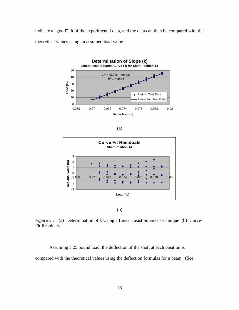
73
indicate a “good” fit of the experimental data, and the data can then be compared with the
theoretical values using an assumed load value.
Determination of Slope (k)Linear Least Squares Curve-Fit for Shaft Position 14
y = 4453.2x - 305.95
R2 = 0.9883
0
10
20
30
40
50
0.068 0.07 0.072 0.074 0.076 0.078 0.08
Deflection (in)
Lo
ad (
lb)
Instron Test Data
Linear Fit (Test Data)
(a)
Curve Fit Residuals Shaft Position 14
-3
-2
-1
0
1
2
3
0.068 0.07 0.072 0.074 0.076 0.078 0.08
Load (lb)
Res
idu
al V
alu
e (i
n)
(b)
Figure 5.1 (a) Determination of k Using a Linear Least Squares Technique (b) Curve-Fit Residuals
Assuming a 25 pound load, the deflection of the shaft at each position is
compared with the theoretical values using the deflection formulas for a beam. (See

74
Figure 5.2) From the figure, it is apparent that the values differ significantly towards the
butt end of the shaft and become closer towards tip.
Comparison of Methods8 inch Span - 25 lb load, Simple Supports
0
0.0002
0.0004
0.0006
0.0008
0.001
0.0012
0 4 8 12 16 20 24 28 32 36
Shaft Position (in)
Mo
men
t o
f In
erti
a (i
n4 )
I_Theoretical
I_Experimental
Figure 5.2 Comparison of Theoretical and Experimental Techniques for theDetermination of the Moment of Inertia for an 8 inch Beam with a Mid-Span Load andSimple Supports
This suggests a problem with the technique, and finite element analysis is used to
examine the problem. Performed at five positions on the shaft, FEA results demonstrated
ovalization of the shaft at the application of the load. This is most likely due to localized
deflection, especially for positions with thin cross-sections compared with the outer
diameter. (See Figure 5.3)

75
Figure 5.3 Exaggerated Ovalization of the Shaft at the Point of Load Application.
With the finite element analysis performed, the FEA results are then compared
with the theoretical and experimental values for deflection. (See Figure 5.4) It is
apparent that the deflection values for experimental and finite element are greater than
values determined by theory. Additionally, the deflections of the experimental and FEA
are similar. Thus, “ovalization” of the shaft is considered a major contributor to large
discrepancies, and additional load conditions are considered using finite element analysis
of the shaft sections.

76
Comparison of Methods8 inch Span - 25 lb Center Load, Simple Supports
0
0.005
0.01
0.015
0.02
0.025
0.03
0 2 4 6 8 10 12 14 16 18 20 22 24 26 28 30 32 34 36
Shaft Position (in)
Def
lect
ion
(in
)
FEA Deflection
Exp Deflection
Theo Deflection
Figure 5.4 Comparison of Deflection Values for Finite Element, Experimental, andTheoretical Methods
The large discrepancy of deflection values establishes the need to evaluate
additional cases, and supplementary loading conditions are examined using FEA. In the
hopes that a longer span would improve results, the span length is increased from 8
inches to 12 inches for the first case. An examination of the percent discrepancies in
Figure 5.5 reveals an improvement with the discrepancies ranging from 25% at the butt
end to 4 % at the tip. Although extension of the span length has reduced the
discrepancies, the values still differ significantly from the theoretical values, and the
effects of localized deflection are still evident. Therefore, other loading conditions must
be examined.

77
Discrepancy of Methods(Theoretical - FEA)
-80
-70
-60
-50
-40
-30
-20
-10
0
0 4 8 12 16 20 24 28 32 36
Shaft Position (in)
Dis
crep
ancy
(%
)8 in Concentrated - S.S.
12 in Concentrated - S.S.
Figure 5.5 Comparison of the percent discrepancies of 8 and 12 inch simply-supportedspan with a 25 lb load applied mid-span.
To circumvent the localized deflection of the concentrated load, distributed
loading cases are examined. A distributed loading case, 25 lb/inch over 1 inch, with
simple supports is first considered, but the discrepancy values are only slightly better than
the 12 inch concentrated load with simple supports. (See Figure 5.6) A distributed load
with 1 inch distributed support is then considered, and the discrepancies are less than the
simply-supported distributed case and range from 4.5% at the butt end to 2.7% at the tip
of the shaft.

78
Discrepancy of Methods(Theoretical - FEA)
-25
-20
-15
-10
-5
0
0 4 8 12 16 20 24 28 32 36
Shaft Position (in)
Dis
crep
ancy
(%
)12 in Distributed - S.S.
12 in Distributed - D.S.
Figure 5.6 Comparison of the percent discrepancies of a 12 inch under a distributed loadwith simply supported and distributed supports.
Based upon the FEA results, experimental testing with the Instron tester is again
performed on the steel shaft, but this time, three one inch blocks are also employed to
simulate the distributed load and support. The applied load and corresponding deflection
is again curve-fit using a least squares technique, and the deflection is compared with the
theoretical values determined using Equation (4.5) on page 58. From Figure 5.7, it is
apparent that the deflections are similar for the majority of the shaft but differ at the ends,
especially the butt end of the shaft. Since the shaft hangs in the three-point bend
apparatus, the force of gravity on the overhanging portion may provide slightly higher
deflections at the butt end and slightly lower deflections at the tip. Unfortunately, tests
could not be performed to confirm these suspicions, but investigation of this possibility is
recommended for further work in the experimental determination of the shaft.

79
Comparison of MethodsSteel Shaft
00.010.020.030.040.050.060.070.08
2 6 10 14 18 22 26 30 34
Shaft Position (in)
Def
lect
ion
(in
)
Experimental
Theoretical
Figure 5.7 Comparison of experimental and theoretical deflections for steel shaft.
The flexural stiffness of the shaft is then determined by rearranging and solving
Equation (4.5) on page 58. Since the cross-section material of the steel shaft is
homogeneous, the moment of inertia is easily determined and compared with the
theoretical values. From Figure 5.8, it is apparent that the results are similar for most of
the shaft.
Comparison of MethodsSteel Shaft
0
0.0002
0.0004
0.0006
0.0008
0.001
0.0012
2 6 10 14 18 22 26 30 34
Shaft Position (in)
Mo
men
t o
f In
erti
a (i
n4 )
Experimental
Theoretical
Figure 5.8 Comparison of experimental and theoretical moments of inertia.
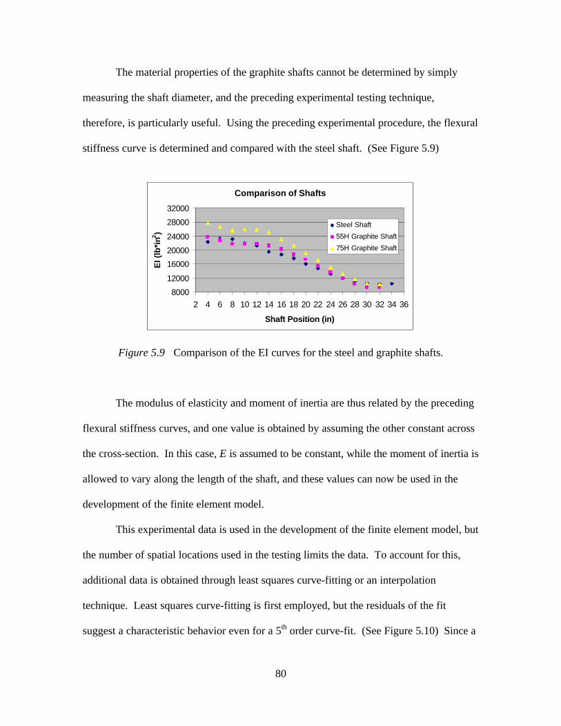
80
The material properties of the graphite shafts cannot be determined by simply
measuring the shaft diameter, and the preceding experimental testing technique,
therefore, is particularly useful. Using the preceding experimental procedure, the flexural
stiffness curve is determined and compared with the steel shaft. (See Figure 5.9)
Comparison of Shafts
8000
12000
16000
20000
24000
28000
32000
2 4 6 8 10 12 14 16 18 20 22 24 26 28 30 32 34 36
Shaft Position (in)
EI (
lb*i
n2)
Steel Shaft
55H Graphite Shaft
75H Graphite Shaft
Figure 5.9 Comparison of the EI curves for the steel and graphite shafts.
The modulus of elasticity and moment of inertia are thus related by the preceding
flexural stiffness curves, and one value is obtained by assuming the other constant across
the cross-section. In this case, E is assumed to be constant, while the moment of inertia is
allowed to vary along the length of the shaft, and these values can now be used in the
development of the finite element model.
This experimental data is used in the development of the finite element model, but
the number of spatial locations used in the testing limits the data. To account for this,
additional data is obtained through least squares curve-fitting or an interpolation
technique. Least squares curve-fitting is first employed, but the residuals of the fit
suggest a characteristic behavior even for a 5th order curve-fit. (See Figure 5.10) Since a

81
“good” curve-fit is unavailable, the additional data is merely interpolated using the
experimentally measured positions.
Determination of Additional DataLeast Squares Curve-Fit for 75H Graphite Shaft
I = -3E-10x5 + 3E-08x4 - 1E-06x3
+ 2E-05x2 - 0.0001x + 0.0013R2 = 0.999
0
0.0002
0.0004
0.0006
0.0008
0.001
0.0012
2 6 10 14 18 22 26 30 34
Shaft Postion (in)
Mo
men
t o
f In
erti
a (i
n4 )
Experimental Data
5th Order Fit
(a)
Curve-Fit Residuals
-0.00002
-0.000015-0.00001
-0.000005
0
0.0000050.00001
0.000015
0.00002
2 6 10 14 18 22 26 30 34
Shaft Position (in)
Res
idu
al V
alu
e (i
n4 )
(b)
Figure 5.10 (a) Fifth order least-squares curve-fit of the experimental moment ofinertia data for the 75H graphite shaft. (b) Corresponding curve-fit residuals.
With the determination of EI, the remaining physical parameters of the shaft are
then determined. As previously stated, each shaft is divided into sections based upon the
taper of the shaft, and the mass and physical dimensions are measured. The mass is
measured using an electronic balance, while the length and diameters of the sections are

82
determined using the calipers. The inner and outer diameters are measured at each
section end using dial calipers, while the values for the interior positions of each section
are then interpolated. Assuming the section is a frustum, the volume of each section is
calculated using Equation (4.6) on page 60, and the weight density is obtained by
dividing the weight by the volume.
Finally, the grip is characterized to account for the effects of its mass on the
system. Using a similar procedure as the shaft, the grip is divided into sections, and the
mass of each section is measured using the electronic balance. The value for the mass at
corresponding shaft locations is then interpolated and used as lumped mass in the finite
element modeling of the system.
Dynamic Analysis Results
The finite element and modal models are developed according to the procedures
outlined in the previous chapters, and the requisite eigenvalues and eigenvectors are
obtained for the desired boundary conditions. Free-free and clamped-free cases are
examined for both, and the mode shapes and frequencies are compared to determine the
degree of correlation, if any between the two methods. Also, an additional case, hands-
free, is investigated solely using modal analysis to ascertain the boundary conditions of a
typical grip.
Once the appropriateness of the FEA is established through correlation, the
dynamic effects of the shaft are examined using the nonlinear dynamic solver in Algor®.
To accomplish this task, previously acquired swing data is calibrated, and the down-
swing portion of the moment curve is then interpolated by a series of lines. These lines

83
are then input into the Accupak utility, and the dynamic response of the club is
determined for the club model.
Modal Data
The coherence is first examined to determine the casuality between the input and
output at each spatial position. As stated previously, the coherence function measures the
linear relationship between the output and input and is defined between 0 and 1, with
unity being total correlation. Figure 5.11b is the driving point coherence for free-free,
steel shaft test and is representative of the coherences. It approaches unity for most
frequencies, but is low at the extremely low frequencies. Since the HP analyzer uses the
H1 estimator, low coherence can occur at anti-resonances, which is the case here.
Examination of the driving point FRF, Figure 5.11a, reveals an anti-resonance at the
extremely low frequency, which is most likely due to rigid body modes.

84
Driving Point FRF Steel Shaft, Free-Free
0.1
1
10
100
1000
0 100 200 300 400 500 600 700 800
Frequency
Am
plit
ud
e (d
B)
(a)
Driving Point FRF Steel Shaft, Free-Free
0
0.2
0.4
0.6
0.8
1
0 100 200 300 400 500 600 700 800
Frequency
Co
her
ence
(b)
Figure 5.11 Steel shaft, free-free driving point FRF. (a) Amplitude (b) Coherence
With the frequency response functions acquired, modal data is input into CADA
PCTM, and the modal parameters are extracted using a MDOF curve-fitting technique in
the software package. The poles, mode frequencies, are then selected, and the
corresponding mode shapes are estimated for each mode. To ensure proper curve-fitting,
an FRF is synthesized by the software and then compared with the original. From Figure
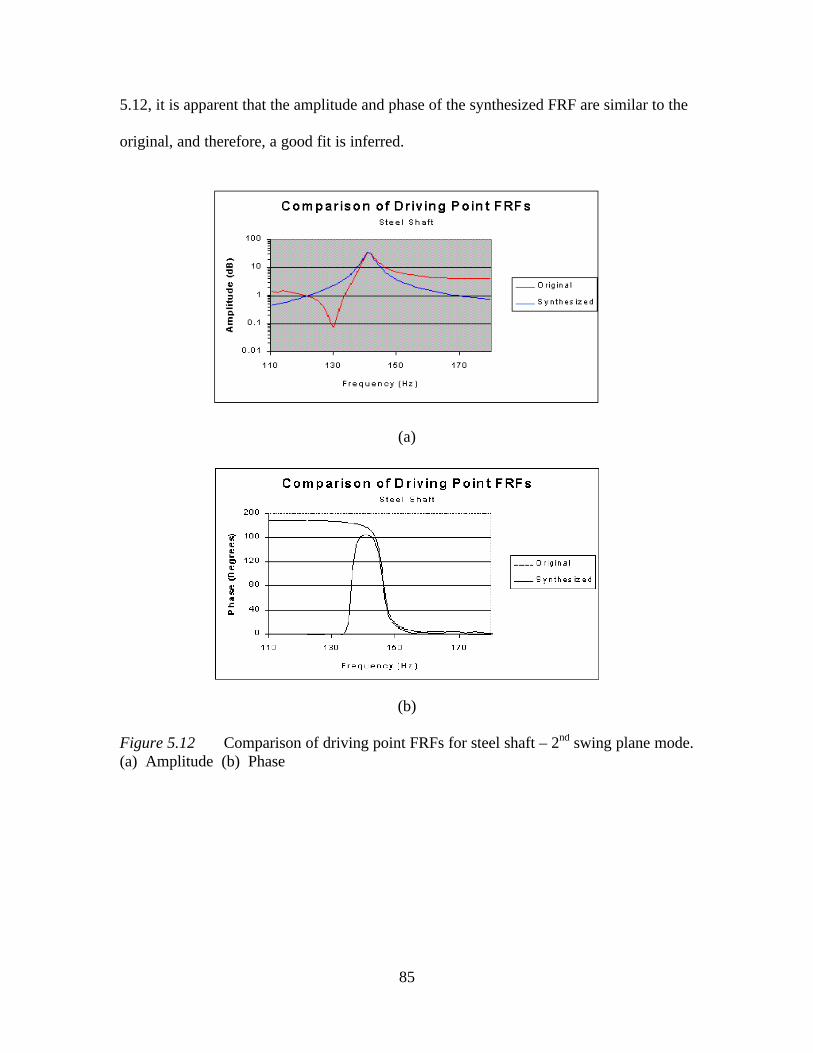
85
5.12, it is apparent that the amplitude and phase of the synthesized FRF are similar to the
original, and therefore, a good fit is inferred.
(a)
(b)
Figure 5.12 Comparison of driving point FRFs for steel shaft – 2nd swing plane mode.(a) Amplitude (b) Phase
86
Comparison and Correlation
Perhaps the most important component of any analysis is the comparison of the
obtained results. After the appropriate values have been garnered, the mass-normalized
mode shapes and frequencies are compared for the desired boundary conditions. This is
first accomplished with a comparison of the mode frequencies and then inspection of the
mode shapes.
Frequency Comparison
The contrasting of frequencies is among the simplest forms of comparing
different analysis methods and provides insight into correlation, or lack there of, between
the techniques. Thus, if two methods are truly similar, the results will agree within a
relatively small discrepancy, while dissimilar values will have larger discrepancies.
Steel Shaft
The finite element and modal frequencies are first compared for the steel shaft.
The finite element and modal frequencies are compared for the free-free and clamped-
free boundary conditions. Examining Table 5.1, it is apparent that the mode frequencies
are similar for both the free-free and clamped-free cases, with the largest discrepancy
occurring at the third droop-plane mode.

87
Table 5.1 : Mode frequencies for steel shaft. (a) Free-Free (b) Clamped-Free
Mode FEA Modal Damping Plane % discrepancy
(Hz) (Hz) % (FEA-Modal)1 42.13 39.73 0.19 Droop 5.692 47.05 46.01 1.12 Swing 2.213 126.92 119.62 0.46 Droop 5.754 143.91 144.01 0.13 Swing -0.075 261.02 243.02 1.16 Droop 6.906 287.98 290.99 1.90 Swing -1.05
(a)
Mode FEA Modal Damping Plane % discrepancy
(Hz) (Hz) % (FEA-Modal)1 5.90 5.70 0.84 Droop 3.352 5.90 5.87 1.17 Swing 0.583 58.01 59.61 1.76 Torsional -2.774 65.82 63.43 0.13 Droop 3.645 83.38 88.94 1.29 Swing -6.676 186.77 169.89 1.90 Droop 9.047 231.92 231.83 1.13 Swing 0.04
(b)
Additionally, another case, hands-free in the swing-plane only, is examined using
modal analysis alone since the exact mechanisms for simulating the finite element
boundary conditions are unknown for this case, and the results are listed in Table 5.2.
The hands-free frequencies are compared against the swing-plane values determined for
the other two boundary cases.
Table 5.2 : Mode frequencies for the hands-free boundary condition for the steel shaft.
Mode Modal Damping
(Hz) %1 50.11 6.362 148.02 3.373 281.56 0.87
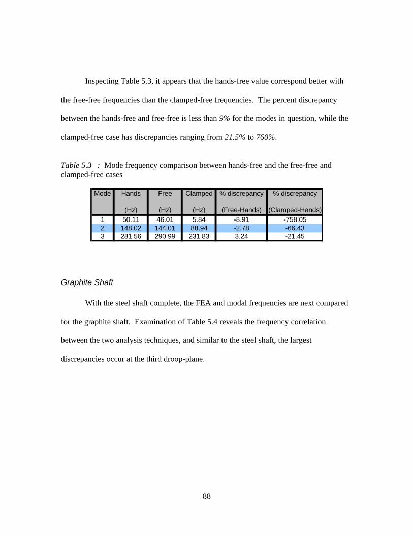
88
Inspecting Table 5.3, it appears that the hands-free value correspond better with
the free-free frequencies than the clamped-free frequencies. The percent discrepancy
between the hands-free and free-free is less than 9% for the modes in question, while the
clamped-free case has discrepancies ranging from 21.5% to 760%.
Table 5.3 : Mode frequency comparison between hands-free and the free-free andclamped-free cases
Mode Hands Free Clamped % discrepancy % discrepancy
(Hz) (Hz) (Hz) (Free-Hands) (Clamped-Hands)1 50.11 46.01 5.84 -8.91 -758.052 148.02 144.01 88.94 -2.78 -66.433 281.56 290.99 231.83 3.24 -21.45
Graphite Shaft
With the steel shaft complete, the FEA and modal frequencies are next compared
for the graphite shaft. Examination of Table 5.4 reveals the frequency correlation
between the two analysis techniques, and similar to the steel shaft, the largest
discrepancies occur at the third droop-plane.

89
Table 5.4 : Mode frequencies for graphite shaft. (a) Free-Free (b) Clamped-Free
Mode FEA Modal Damping Plane % discrepancy
(Hz) (Hz) % (FEA-Modal)7 48.01 46.38 1.13 Droop 3.398 52.61 50.99 0.97 Swing 3.099 136.62 128.57 0.54 Droop 5.89
10 155.81 156.04 0.29 Swing -0.1511 282.91 262.68 1.05 Droop 7.1512 309.56 313.22 0.50 Swing -1.18
(a)
Mode FEA Modal Damping Plane % discrepancy
(Hz) (Hz) % (FEA-Modal)1 5.90 5.76 0.58 Droop 2.352 5.91 5.84 0.59 Swing 1.123 58.32 53.69 1.19 Torsional 7.944 69.56 67.17 1.57 Droop 3.445 91.63 94.66 0.74 Swing -3.316 209.40 190.35 1.41 Droop 9.107 257.70 262.00 0.73 Swing -1.67
(b)
The hands-free case is also examined for the graphite shaft, and the resulting
frequency values, Table 5.5, are once more compared with the free-free and clamped-free
boundary conditions. From Table 5.6, it once again appears that the free-free values
appear to correlate better with the hands-free frequencies than with the clamped-free
frequencies.

90
Table 5.5 : Mode frequencies for the hands-free boundary condition for the steel shaft.
Mode Modal Damping
(Hz) %1 54.01 5.712 158.02 3.373 302.65 0.74
Table 5.6 : Mode frequency comparison between hands-free and the free-free andclamped-free cases
Mode Hands Free Clamped % discrepancy % discrepancy
(Hz) (Hz) (Hz) (Free-Hands) (Clamped-Hands)1 54.01 50.99 5.84 -5.92 -824.832 158.02 156.04 94.66 -1.27 -66.933 302.65 313.22 262.00 3.37 -15.52
Mode Shape
With the mode frequency comparison complete, the mode shapes of the different
techniques are contrasted. This is first accomplished by visual inspection of the mode
shapes for the plane of interest, the droop and swing planes in this case. With visual
similarities established, the eigenvectors are then compared numerically using the Modal
Assurance Criterion, which is discussed in Chapter 3.
Since the mode shapes are similar for both the graphite and steel shafts, a detailed
examination of the steel shaft is discussed in the ensuing sections. Conversely, the
graphite shaft will only be covered tersely in the subsequent discussion of results, but all
mode shapes are included in the appendix of this work.

91
Steel Shaft
Free-free and clamped-free cases are examined using both modal and finite
element analysis, and the mode shapes and frequencies are compared to determine the
degree of correlation, if any between the two methods. Also, an additional case, hands-
free, is investigated solely using modal analysis to ascertain the boundary conditions of a
typical grip.
The examination of mode shapes is first accomplished with a visual inspection of
the mode shapes. When visual similarity has been established, the mode shapes are then
numerically compared using the MAC, and the values range from 0 to 1, with unity again
being total correlation and zero representing no correlation.
Free-Free
The free-free boundary condition is typically utilized in structural dynamic
analysis since it is among the easiest to simulate in finite element and modal analysis.
Therefore, it is the first case examined by visual inspection and the MAC.

92
Visual inspection of the droop (Figure 5.13) and swing (Figure 5.14) planes
reveals similarities between the finite element and EMA mode shapes. Additionally,
closer examination of the figures reveals particularly close visual correlation for the
second swing mode (Figure 5.14b), while the second droop (Figure 5.13b) and the third
swing mode (Figure 5.14c) exhibit a greater discrepancy.
This slight discrepancy is to be expected due to the nature of the analysis
methods. The finite element analysis is analytical technique and therefore yields the
smoothed mode shapes exhibited in the two figures. Conversely, the modal analysis is an
experimental technique, and the eigenvectors are obtained by curve-fitting data obtained
through testing. Thus, the results are not the “smoothed” mode shapes predicted by
analytical and theoretical techniques.
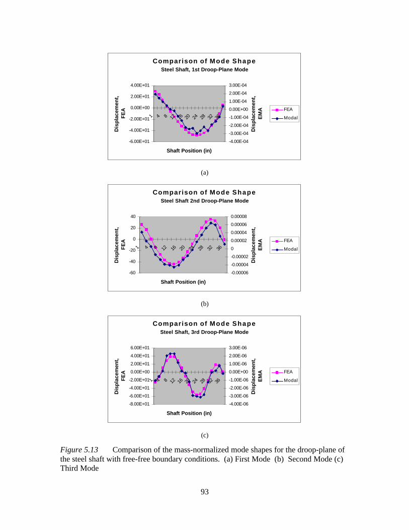
93
Comparison of Mode ShapeSteel Shaft, 1st Droop-Plane Mode
-6.00E+01
-4.00E+01
-2.00E+01
0.00E+00
2.00E+01
4.00E+01
1 4 8 12 16 20 24 28 32 36
Shaft Position (in)
Dis
pla
cem
ent,
F
EA
-4.00E-04
-3.00E-04
-2.00E-04
-1.00E-04
0.00E+00
1.00E-04
2.00E-04
3.00E-04
Dis
pla
cem
ent,
E
MA FEA
Modal
(a)
Comparison of Mode ShapeSteel Shaft 2nd Droop-Plane Mode
-60
-40
-20
0
20
40
1 4 8 12 16 20 24 28 32 36
Shaft Position (in)
Dis
pla
cem
ent,
F
EA
-0.00006
-0.00004
-0.00002
0
0.00002
0.00004
0.00006
0.00008
Dis
pla
cem
ent,
E
MA FEA
Modal
(b)
Comparison of Mode ShapeSteel Shaft, 3rd Droop-Plane Mode
-8.00E+01
-6.00E+01
-4.00E+01
-2.00E+01
0.00E+00
2.00E+01
4.00E+01
6.00E+01
1 4 8 12 16 20 24 28 32 36
Shaft Position (in)
Dis
pla
cem
ent,
F
EA
-4.00E-06
-3.00E-06
-2.00E-06
-1.00E-06
0.00E+00
1.00E-06
2.00E-06
3.00E-06
Dis
pla
cem
ent,
E
MA FEA
Modal
(c)
Figure 5.13 Comparison of the mass-normalized mode shapes for the droop-plane ofthe steel shaft with free-free boundary conditions. (a) First Mode (b) Second Mode (c)Third Mode

94
Comparison of Mode ShapeSteel Shaft, 1st Swing-Plane Mode
-4.00E+01
-2.00E+01
0.00E+00
2.00E+01
4.00E+01
6.00E+01
1 4 8 12 16 20 24 28 32 36
Shaft Position (in)
Dis
pla
cem
ent,
F
EA
-6.00E-05
-4.00E-05
-2.00E-05
0.00E+00
2.00E-05
4.00E-05
6.00E-05
8.00E-05
Dis
pla
cem
ent,
E
MA FEA
Modal
(a)
Comparison of Mode ShapeSteel Shaft, 2nd Swing-Plane Mode
-6.00E+01
-4.00E+01
-2.00E+01
0.00E+00
2.00E+01
4.00E+01
6.00E+01
1 4 8 12 16 20 24 28 32 36
Shaft Position (in)
Dis
pla
cem
ent,
F
EA
-6.00E-05
-4.00E-05
-2.00E-05
0.00E+00
2.00E-05
4.00E-05
6.00E-05
Dis
pla
cem
ent,
E
MA FEA
Modal
(b)
Comparison of Mode ShapeSteel Shaft, 3rd Swing-Plane Mode
-6.00E+01
-4.00E+01
-2.00E+01
0.00E+00
2.00E+01
4.00E+01
6.00E+01
1 4 8 12 16 20 24 28 32 36
Shaft Position (in)
Dis
pla
cem
ent,
F
EA
-3.00E-07
-2.00E-07
-1.00E-07
0.00E+00
1.00E-07
2.00E-07
3.00E-07
Dis
pla
cem
ent,
E
MA FEA
Modal
(c)
Figure 5.14 Comparison of the mass-normalized mode shapes for the swing-plane ofthe steel shaft with free-free boundary conditions. (a) First Mode (b) Second Mode (c)Third Mode

95
With the visual correlation established, the mode shapes are then compared
numerically using the modal assurance criterion. The diagonal values are the primary
interest of the comparison since a value close to unity implies “good” correlation between
the compared eigenvectors, while the off-diagonal terms compare the relationship
between different modes.
Examination of the MACs (Table 5.7) reveals diagonal values of 0.9 or greater
with the exception of the third swing mode, which has a value of 0.88. Using the visual
method (Figure 5.14c), it is apparent that the displacements are less than expected for a
few spatial locations (positions 20 and 22) near the middle of the club. The exact nature
of this discrepancy is unknown, and it may just be the nature of the test and the curve-
fitting. To examine these possibilities, future work, with focus on the curve-fitting and
data acquisition, must be performed.
Although not unity, these diagonal MAC values suggest “good” correlation
between the finite element and modal mode shapes even for the third swing mode. It is
also notable that the first and third droop planes exhibit some similarity, roughly 0.25 or
25 percent, and visual inspection implies a small degree of likeness as well.

96
Table 5.7 : Free-Free MAC for steel shaft (a) Droop-plane (b) Swing Plane
1 2 3
1 0.9667 0.0244 0.2671
2 0.0003 0.9038 0.0632
3 0.2577 0.0624 0.9559
Modal
FEA
Mode
Mode
(a)
1 2 3
1 0.9469 0.0718 0.1652
2 0.0224 0.9227 0.0539
3 0.0836 0.0037 0.8873
Modal
FEA
Mode
Mode
(b)
Clamped-Free
The clamped-free is the one most often employed in finite element analysis of the
golf club, and it is typically used to simulate the effects of the players grip in dynamic
analysis. Since one of the objectives of this work is to establish the boundary conditions
of the hands, visual inspection and the use of the MAC are again utilized to contrast the
FEA and EMA mode shapes. Visual inspection of the two planes (Figure 5.15 and
Figure 5.16) reveals similarities between the finite element and modal mode shapes,
particularly for the first droop and swing plane modes

97
Comparison of Mode ShapeSteel Shaft, 1st Droop-Plane Mode
-3.00E+01
-2.50E+01
-2.00E+01
-1.50E+01
-1.00E+01
-5.00E+00
0.00E+0010 14 18 22 26 30 34
Shaft Position (in)
Dis
pla
cem
ent,
F
EA
-8.00E-01
-6.00E-01
-4.00E-01
-2.00E-01
0.00E+00
Dis
pla
cem
ent,
E
MA FEA
Modal
(a)
Comparison of Mode ShapeSteel Shaft, 2nd Droop-Plane Mode
-6.00E+01
-5.00E+01
-4.00E+01
-3.00E+01
-2.00E+01
-1.00E+01
0.00E+00
1.00E+01
10 14 18 22 26 30 34
Shaft Position (in)
Dis
pla
cem
ent,
F
EA
-2.50E-03
-2.00E-03
-1.50E-03
-1.00E-03
-5.00E-04
0.00E+00
5.00E-04
Dis
pla
cem
ent,
E
MA FEA
Modal
(b)
Comparison of Mode ShapeSteel Shaft, 3rd Droop-Plane Mode
-4.00E+01
-2.00E+01
0.00E+00
2.00E+01
4.00E+01
6.00E+01
8.00E+01
10 14 18 22 26 30 34
Shaft Position (in)
Dis
pla
cem
ent,
F
EA
-1.00E-04
-5.00E-05
0.00E+00
5.00E-05
1.00E-04
1.50E-04
2.00E-04
Dis
pla
cem
ent,
E
MA FEA
Modal
(c)
Figure 5.15 Comparison of the mass-normalized mode shapes for the droop-plane ofthe steel shaft with clamped-free boundary conditions. (a) First Mode (b) Second Mode(c) Third Mode

98
Comparison of Mode ShapeSteel Shaft, 1st Swing-Plane Mode
-3.00E+01
-2.50E+01
-2.00E+01
-1.50E+01
-1.00E+01
-5.00E+00
0.00E+0010 14 18 22 26 30 34
Shaft Position (in)
Dis
pla
cem
ent,
F
EA
-8.00E-01
-6.00E-01
-4.00E-01
-2.00E-01
0.00E+00
Dis
pla
cem
ent,
E
MA FEA
Modal
(a)
Comparison of Mode ShapeSteel Shaft, 2nd Swing-Plane Mode
-6.00E+01
-5.00E+01
-4.00E+01
-3.00E+01
-2.00E+01
-1.00E+01
0.00E+00
1.00E+01
10 14 18 22 26 30 34
Shaft Position (in)
Dis
pla
cem
ent,
F
EA
-2.50E-03
-2.00E-03
-1.50E-03
-1.00E-03
-5.00E-04
0.00E+00
5.00E-04
Dis
pla
cem
ent,
E
MA FEA
Modal
(b)
Comparison of Mode ShapeSteel Shaft, 3rd Swing-Plane Mode
-8.00E+01
-6.00E+01
-4.00E+01
-2.00E+01
0.00E+00
2.00E+01
4.00E+01
6.00E+01
10 14 18 22 26 30 34
Shaft Position (in)
Dis
pla
cem
ent,
F
EA
-6.00E-04
-4.00E-04
-2.00E-04
0.00E+00
2.00E-04
4.00E-04
6.00E-04
Dis
pla
cem
ent,
E
MA FEA
Modal
(c)
Figure 5.16 Comparison of the mass-normalized mode shapes for the droop-plane ofthe steel shaft with clamped-free boundary conditions. (a) First Mode (b) Second Mode(c) Third Mode

99
The mode shapes are then compared using the MAC, and for both planes,
examination of the MAC (Table 5.8) reveals “high” correlation between the finite
element analysis and modal analysis. In fact, the diagonal values are above 0.97 or 97 %
for the droop plane, while 0.946, or 94.6%, is the lowest for the swing-plane. Upon first
glance, these values seem unreasonably “high”, especially after the visual comparison has
been completed, but after further consideration, these values appear more feasible.
The two lowest diagonal values of the MAC occur at the third mode for both
droop and swing planes, and these mode shapes are more closely examined. From Figure
5.15c and Figure 5.16c, it first appears as though the two mode shapes differ
significantly, but the scale of the figures is different from the free-free mode shape scale.
For the free-free mode shapes, spatial locations from 4 to 34 are examined, while the
number of location is limited to spatial location from 10 to 34 because the grip is clamped
in the vise. Thus, a small difference in mode shape visually appears to be a larger one.

100
Table 5.8 : Clamped-Free MAC for steel shaft (a) Droop-plane (b) Swing Plane
1 2 3
1 0.9976 0.6812 0.0380
2 0.6701 0.9903 0.4355
3 0.0190 0.3341 0.9782
Modal
FEA
Mode
Mode
(a)
1 2 3
1 0.9986 0.6860 0.0316
2 0.6744 0.9955 0.0769
3 0.1353 0.0022 0.9464
Modal
FEA
Mode
Mode
(b)
It is also interesting to note the “high” degree of correlation, greater than 67%,
between the first and second modes for both planes. Although this seems unusual, visual
inspection of the FEA mode shapes reveals the similarity. From Figure 5.17, it is
apparent that the two modes have comparable shapes, particularly for spatial location’s 4
to 20.

101
Comparison of Mode ShapeSteel Shaft, Droop-Plane Modes
-3.00E+01
-2.50E+01
-2.00E+01
-1.50E+01
-1.00E+01
-5.00E+00
0.00E+00
10 14 18 22 26 30 34
Shaft Position (in)
Dis
pla
cem
ent,
1s
t M
od
e
-6.00E+01
-5.00E+01
-4.00E+01
-3.00E+01
-2.00E+01
-1.00E+01
0.00E+00
1.00E+01
Dis
pla
cem
ent,
2n
d M
od
e 1st Droop -FEA
2nd Droop -FEA
Figure 5.17 Comparison of first and second droop modes for the steel shaft.
Comparison of Hands-Free versus Free-Free and Clamped-Free
The hands-free is the final case examined and is employed to simulate the
boundary conditions due to the gripping of the golf club. In this case, the club is gripped,
the face is struck by a modal impact hammer, and the corresponding response is captured.
The resulting FRFs are then curve-fit to determine the frequencies and mode shapes, and
the eigenvalues and eigenvectors are then compared with the free-free and clamped-free
cases to determine any similarities.
The hands-free case is first visually compared with the free-free case to examine
any correlation. (See Figure 5.18) Although the number of spatial locations is limited by
the grip of the hands, it is apparent that the hands-free and free-free mode shapes are
similar, especially for the first and second modes.

102
Comparison of Mode ShapeSteel Shaft, 1st Swing-Plane Mode
-6.00E-05
-4.00E-05
-2.00E-05
0.00E+00
2.00E-05
4.00E-05
6.00E-05
8.00E-05
0 6 12 18 24 30 36
Shaft Position (in)
Dis
pla
cem
ent
-1.00E+00
-5.00E-01
0.00E+00
5.00E-01
1.00E+00
1.50E+00
2.00E+00
2.50E+00
Dis
pla
cem
ent
Free-Free
Hands
(a)
Comparion of Mode ShapeSteel Shaft, 2nd Swing-Plane
-6.00E+01
-4.00E+01
-2.00E+01
0.00E+00
2.00E+01
4.00E+01
6.00E+01
0 6 12 18 24 30 36
Shaft Position (in)
Dis
pla
cem
ent
-1.00E-04
-5.00E-05
0.00E+00
5.00E-05
1.00E-04
Dis
pla
cem
ent
Free-Free
Hands
(b)
Comparison of Mode ShapeSteel Shaft, 3rd Swing-Plane
-3.00E-07
-2.00E-07
-1.00E-07
0.00E+00
1.00E-07
2.00E-07
3.00E-07
0 4 8 12 16 20 24 28 32 36
Shaft Position (in)
Dis
pla
cem
ent
-1.50E+00
-1.00E+00
-5.00E-01
0.00E+00
5.00E-01
1.00E+00
Dis
pla
cem
ent
Free-Free
Hands
(c)
Figure 5.18 Comparison of the mass-normalized mode shapes for the swing-plane ofthe steel shaft with free-free versus hands-free boundary conditions. (a) First Mode (b)Second Mode (c) Third Mode

103
After the free-free and hands-free cases have been compared, the relationship
between the clamped-free and hands-free is then investigated. (See Figure 5.19) The
mode shapes may initially appear to be alike, but closer inspection, especially at the first
spatial location, reveals the dissimilarity between the mode shapes.
Examining the first mode shape, it is apparent the mode shapes are different at the
spatial locations for the upper (butt end) half of the shaft. This is particularly evident for
the first spatial location, which differs significantly between the two modes. For the
clamped-free case, the first spatial location is obviously clamped and thus has zero
displacement, while the corresponding location in the hands-free case obviously has a
relative displacement.
The second and third modes also appear to have an initial resemblance, especially
for the second half (tip end) of the shaft, but further examination, with particular attention
to the first spatial location, exposes the differences between the two boundary conditions.
As previously noted, the clamped-case limits the first location displacement to zero, but
the relative displacements of the corresponding location are obviously for the hands-free
mode.

104
Comparison of Mode ShapeSteel Shaft, 1st Swing-Plane Mode
-8.00E-01
-6.00E-01
-4.00E-01
-2.00E-01
0.00E+000 6 12 18 24 30 36
Shaft Position (in)
Dis
pla
cem
ent
-1.00E+00
-5.00E-01
0.00E+00
5.00E-01
1.00E+00
1.50E+00
2.00E+00
2.50E+00
Dis
pla
cem
ent
Clamped-Free
Hands
(a)
Comparion of Mode ShapeSteel Shaft, 2nd Swing-Plane
-2.50E-03
-2.00E-03
-1.50E-03
-1.00E-03
-5.00E-04
0.00E+00
5.00E-04
0 4 8 12162024 283236
Shaft Position (in)
Dis
pla
cem
ent
-1.00E-04
-5.00E-05
0.00E+00
5.00E-05
1.00E-04
Dis
pla
cem
ent
Clamped-Free
Hands
(b)
Comparison of Mode ShapeSteel Shaft, 3rd Swing-Plane Mode
-6.00E-04
-4.00E-04
-2.00E-04
0.00E+00
2.00E-04
4.00E-04
6.00E-04
0 6 12 18 24 30 36
Shaft Position (in)
Dis
pla
cem
ent
-1.50E+00
-1.00E+00
-5.00E-01
0.00E+00
5.00E-01
1.00E+00
Dis
pla
cem
ent
Clamped-Free
Hands
(c)
Figure 5.19 Comparison of the mass-normalized mode shapes for the swing-plane ofthe steel shaft with clamped-free versus hands-free boundary conditions. (a) First Mode(b) Second Mode (c) Third Mode

105
The visual inspection of the mode shapes establishes the similarity of the free-free
and hands-free mode shapes and exposes the disparity between the clamped-free and
hands-free eigenvectors. Therefore, the free-free and hands-free are only compared using
the modal assurance criterion, which confirms the high degree of correlation.
Examining the MAC – Table 5.9, the “high” correlation between the two cases is
confirmed by the diagonal values, which are greater than 0.9 or 90%, and the
comparatively low off-diagonal terms. These values, combined with the frequency
comparison, indicate strong similarity between the free-free and hands-free case; hence it
can be confidently inferred that gripping of the club produces a boundary condition that is
intrinsically a free-free case.
Table 5.9 : Free-free versus hand-free MAC for steel shaft
1 2 3
1 0.9603 0.0036 0.1066
2 0.0023 0.9896 0.0061
3 0.2460 0.0251 0.9071
Hands
Free
Mode
Mode
Graphite Shaft
Since the mode shapes are similar for both the graphite and steel shafts, the steel
shaft is examined in detail in the previous sections, and the graphite results are now

106
briefly examined. The free-free and clamped-free are again analyzed using both FEA and
EMA, and EMA is again employed to analyze the hands-free conditions.
The eigenvectors are again determined using a MDOF curve-fitting technique,
and the resulting mode shapes are correlated using the same procedure as the steel shaft.
The resulting MACs are included in the subsequent sections, but for the sake of brevity,
the visual comparisons of the mode shapes are included in the appendix of this work.
Free-Free
The free-free eigenvectors are again contrasted visually (See Appendix.) to
determine similarity. With the visual comparison complete, the droop and swing plane
mode shapes are then contrasted numerically using the modal assurance criterion.
Examination of the MACs (Table 5.10) reveals diagonal values of 0.9 or greater
with the exception of the third swing mode, which has a value of 0.887 or 87%. This
correlation value is similar to the value determined for the steel shaft, and thus reinforces
the concerns, and need for future investigation, that are noted in the foregoing steel shaft
section.

107
Table 5.10 : Free-Free MAC for graphite shaft. (a) Droop Plane (b) Swing Plane
1 2 3
1 0.9655 0.2623 0.0853
2 0.0696 0.9628 0.0589
3 0.2530 0.0614 0.9591
Modal
FEA
Mode
Mode
(a)
1 2 3
1 0.9469 0.0718 0.1652
2 0.0224 0.9227 0.0539
3 0.0836 0.0037 0.8873
Modal
FEA
Mode
Mode
(b)
Clamped-Free
The clamped-free is typically employed in finite element of the shaft, and the
resulting mode shapes are once more compared by visual inspection (See Appendix).
This reveals similarities between the finite element and modal mode shapes, and the
mode shapes are thus compared using the MAC.
Inspection of the MAC (Table 5.11) reveals a “high” correlation between the
finite element analysis and modal analysis mode shapes. While not as “high” as the steel
shaft, the diagonal values are above 0.978 or 97.8% for the droop plane, and 0.945, or
94.5%, is the lowest for the swing-plane. These values may once again seem
unreasonably “high” after the visual inspection, but as previously noted, the visual

108
discrepancy appear larger because of the different scaling for the clamped-free and free-
free boundary conditions.
Table 5.11 : Clamped-Free MAC for graphite shaft. (a) Droop Plane (b) Swing Plane
1 2 3
1 0.9949 0.8689 0.2057
2 0.7225 0.9780 0.6411
3 0.2418 0.6176 0.9872
Modal
FEA
Mode
Mode
(a)
1 2 3
1 0.9972 0.7981 0.0029
2 0.7216 0.9914 0.2389
3 0.0278 0.0621 0.9455
Modal
FEA
Mode
Mode
(b)
Comparison of Hands-Free versus Free-Free and Clamped-Free
With the prevalence of graphite shafts in the market, the hands-free is also
investigated for this shaft material and is utilized to simulate the boundary conditions due
to the gripping of the golf club. The testing and parameter extractions are the same as
previously stated, and the resulting eigenvalues and eigenvectors are again contrasted
with the free-free and clamped-free case to investigate any similarities.
The hands-free case is first visually compared with the free-free and clamped-free
cases to examine any correlation between the boundary conditions. (See Appendix), and

109
as expected, the correlation is similar to the steel shaft. Examining the figures, it is also
evident that the hands-free correlates “better” with the hands-free case than the clamped-
free case, and therefore, only the free-free and hands-free are compared using the MAC.
Inspecting the MAC –Table 5.12, the “high” correlation between the two cases is
confirmed by the diagonal values, which are greater than 0.91 or 91%, and the
comparatively low off-diagonal terms. These values, combined with the foregoing
frequency comparison, reinforce the inference made for the steel shaft. Namely, the
gripping of the club produces a boundary condition that is essentially a free-free case.
Table 5.12 : Free-free versus hand-free MAC for graphite shaft
1 2 3
1 0.9728 0.0668 0.2437
2 0.0100 0.9114 0.0001
3 0.2394 0.1068 0.9154
Hands
Free
Mode
Mode
Nonlinear Dynamic Analysis
With the finite element and modal analysis correlated, the large displacement
nonlinear dynamic response of the shaft is then investigated using Algor®. Previously
acquired strain gage data has been taken during an actual club swing. The moment strain
in the shaft at the gage location may be assumed to be an approximation of the applied
moment from the golfer’s hands. The moment strain may be calibrated to get the applied
moment on the shaft. The moment curve for the down swing portion is then interpolated
by a series of line segments. These lines are then input into the nonlinear solver, and the
dynamic response of the club is determined for the club model.

110
Determination of Moment Curve
The input moment curve for the swing is determined by calibrating strain,
obtained using strain gauges, and converting the data. Using previously acquired strain
data, the strain gauge is first calibrated for a flexible and stiff steel shaft (Figure 5.20),
and the input moment curve is then obtained by converting strain data for a typical swing
curve (Figure 5.21).
Calibration of Strain GaugesSteel Shafts
S = 385.85M - 15.64
S = 341.55M - 6.2771
0
100
200
300
400
500
600
0 0.2 0.4 0.6 0.8 1 1.2 1.4 1.6Strain (V)
Mo
men
t (l
b*i
n)
Strain FlexibleStrain Stiff
Linear (Strain Flexible)Linear (Strain Stiff)
Figure 5.20 Calibration of strain gauges for two steel shafts.

111
Moment CurveAveraged Swing Data, Swing-Plane
-150
-100
-50
0
50
100
150
200
250
-2 -1.5 -1 -0.5 0 0.5 1
Time (sec)
Mo
men
t (l
bf*
in)
Figure 5.21 Moment for curve for the swing-plane.
With the data converted, a piecewise linear curve for the swing is then constructed
by selecting a number representative points from the moment curve to linearly
approximate the moment curve. To accomplish this task, the curve is initially simulated
using eight points, while the second, and final, approximation employs 14 points. (See
Figure 5.22) These event curves are then input into the Accupak software utility, and the
finite element is then solved until the software determines convergence.

112
Development of Piecewise Linear Curves
-150
-100
-50
0
50
100
150
200
-0.8 -0.7 -0.6 -0.5 -0.4 -0.3 -0.2 -0.1 0
Time (sec)
Mo
men
t (l
b*i
n)
Average
1st Fit
2nd Fit
Figure 5.22 Development of Accupak event curve using consecutive linearapproximations.
Dynamic Response
The model is solved until convergence has been attained for the desired time
steps, and the response of the golf shaft is then investigated. Examining Figure 5.23, it is
interesting to note the shaft displacement at each time step during the swing. The shaft
and club-head are initially inline, but the club-head soon starts to “lag” the shaft.
Although this “lagging” continues through the downswing, the head begins to “catch” the
shaft midway through the down-swing and barely “lags” the shaft at impact.

113
Figure 5.23 Dynamic swing results obtained using Accupak software utility in Algor.
Summary of Results and Conclusions
The primary objectives of this research are three-fold: 1) the development and
correlation of an appropriate finite element model, 2) the characterization of the hands-
free boundary condition and 3) the examination of the golf club swing dynamics. A finite
element model is developed the using experimentally determined physical parameters.
The model is then solved and correlated with results from the experimental modal
analysis, while a separate modal case is used to determine the boundary conditions

114
caused by the gripping of the club. With the modes correlated, the shaft down-swing is
simulated on the computer.
Summary of Results
The physical parameters of the club-head and golf shaft are determined
experimentally, and then used to develop the finite element model. The club-head center
of gravity is determined using elementary statics, and using the pendulum technique
developed by Johnson (2), the moments of inertia are calculated for the axes of interest.
For the golf shaft, the desired physical parameters are determined through
measurement of the shaft dimensions and three-point bend testing on the Instron tester.
For the Instron testing, it is important to note the effects of localized deflection (See
Figure 5.3) for the concentrated load case with simple supports. The applied load causes
the shaft to ovalize at the point of application and causes the results to differ significantly
from the theoretical.
Finite element analysis, using plate elements, is then performed to examine
alternative testing techniques. The effects of increasing span length, as well as different
loading conditions and supports, are examined. Examining the results, the closest testing
results to theory came by using the 12-inch span beam with a distributed load and
distributed supports. The discrepancies for this case are relatively low, less 5%.
This case is therefore simulated using three 1-inch blocks in the three-point bend
apparatus and Instron tester, and the resulting experimental deflections are comparable to
theory. The EI curves can then be determined, and the values for either the moment of
inertia or modulus of elasticity are determined by holding one constant while the other
115
varies. Here, E is assumed constant for both the graphite and steel shafts, while the
moment of inertia is allowed to vary along the length of the shaft.
Using these physical parameters, the finite element model is analyzed for two
boundary conditions – free-free and clamped-free. These cases are solved until
convergence, and the mode frequencies and shapes are then visually and numerically
correlated with the values extracted from the modal analysis. Visually comparing the
mode shapes (Figure 5.13 to Figure 5.19), it is evident that the finite element and
experimental mode shapes are quite similar. This is further confirmed by the diagonal
values of the MACs, which are about 0.9% or better.
One additional modal case, the hands-free, is performed to ascertain the boundary
conditions due to gripping of the club. When this case is visually compared with the
free-free and clamped-free cases, the hands-free mode shapes correspond with the free-
free case, rather than the clamped-free case. This is confirmed by the values of the MAC,
and it can then be inferred that the hands-free is close to a damped free-free boundary
condition.
With the FEA and modal analysis correlated, the dynamic response of the club
during the down-swing is then computed by analyzing finite element model with the
Accupak software. By converting previously acquired strain data, a moment curve is
determined, and an event curve is established by linearly approximating the moment
curve.
Examining Figure 5.23, it is interesting to note the shaft displacement during
the displayed swing positions. Initially, the shaft and club-head are inline, but club-head
soon starts to “lag” the shaft. This “lagging” continues throughout the downswing, but

116
the head begins to “catch” the shaft midway through the down-swing and “lags” the shaft
slightly at impact.
Future Work
This thesis is the culmination of a great amount of research and analysis, but it is
not the completion of this research. It is merely the beginning, and opportunities abound
for continued work for this project, especially in a few key areas.
The finite element model of the club-head is the first area of opportunity for
continued work. In this research, the club-head was modeled as a lumped mass at the
center of gravity, and the solver did not consider the moments of inertia. To better
characterize the club and its mass distribution, a solver that considers the moments of
inertia must be used, or the club-head could be model using either shell or solid elements.
Additionally, modeling the club-head with either shell or solid elements allows
for the comparison of the club-face mode shapes with the results from experimental
analysis. This would aid in the examination of the club-face node line and the
relationship of the “sweet spot” with the center of gravity.
The characterization of the shaft flexural stiffness is another opportunity for
continued research. In this project, the flexural stiffness was determined at discrete
points using a distributed load simulated by a three-point apparatus and three 1-inch bars,
but this technique limits the number of points examined. To better represent the flexural
stiffness, alternative loading techniques may need to be examined.
A third area of future work concerns the analysis of the golf club during the
backswing and downswing. For this work, only the down-swing of golf club was

117
simulated using a nonlinear dynamic solver, and the analysis was based upon an event
curve of a limited number of points and was not correlated with experimental results.
To improve the analysis, experimental model analysis must be performed on the
club during the swing and through the impact. To accomplish this, different response
transducers and bonding techniques must be used. Additionally, the number of event
curve points must be increased to better represent the actual swing in the dynamic
simulation.

118
References
1. Cochran, A. and Stobbs, J. The search for the perfect swing. Heinemann Press, 1968
2. Thomas, G., Deiters, T., and Best, C. “Simulating golf club performance using modalanalysis.” Proceedings of 13th International Modal Analysis Conference, v 1, SEM,Nashville, TN, 1995, p 989-995
3. Twigg, M. and Butler, J. “Determining the central principal inertia dyadic of a golfclub head. Experimental Techniques, V 20, n 5, p 13-18
4. Johnson, S. “Experimental determination of inertia ellipsoids”. Science and Golf II:Proceedings of the World Scientific Congress of Golf, Chapman and Hall, London,1994, p 290 – 295
5. Swider, P. and Ferraris, G. “Theoretical and experimental dynamic behavior of a golfclub made of composite materials.” Modal Analysis: The International Journal ofAnalytical and Experimental Modal Analysis, V 9, n 1, January 1994, p 57-69
6. Okubo, N. and Simada, M. “Application of CAE (computer-aided engineering) togolf club dynamics Proceedings of the First World Scientific Congress of Golf,Chapman and Hall, London, 1990, p 270 – 273
7. Friswell, M., Smart, M. and Mottershead, J. “Updating finite element models of golfclubs”, Proceedings of 15th International Modal Analysis Conference, v 1, SEM,Bethel, CT, 1997, p 155-161
8. Budney, D and Bellows, D. “A dynamic model for the golf swing”. Paper presented5th International Congress of Sports Sciences, Edmonton, Canada, 1978
9. Budney, D and Bellows, D. “Kinetic analysis of a golf swing”. Research Quarterly,V 50, n 2, 1979, p 171-179
10. Schilansl, N. “Bending frequency of a rotating cantilever beam.” ASME Journal ofApplied Mechanics, V 25, 1958, p 28-30

119
11. Roa, J and Carnegie, W. “Nonlinear vibrations of rotating cantilever beams”, TheAeronautical Journal of the Royal Aeronautical Society, V 74, p 161-165
12. Pnuelli, D. “Natural bending frequency comparable to rotation frequency in rotatingcantilever beam” ASME Journal of Applied Mechanics, V 39, p 602-604
13. Christensen, E. and Lee, S. “Nonlinear finite element modeling of the dynamics ofunrestrained flexible structure” Computers and Structures, V 23, n 6, 1986, p 819-829
14. Yoo, H., Ryan, R. and Scott, R. “Dynamics of flexible beams undergoing overallmotions” Journal of Sound and Vibration, V 181, n 2, 1995, p 261-278
15. Bhat, R. “Transverse vibrations of a rotating uniform beam with tip mass aspredicted by using beam characteristic orthogonal polynomials in the Raleigh-RitzMethod” Journal of Sound and Vibration, V 105, 1986, p 199-210
16. Hoa, S. “Vibration of rotating beam with tip Mass.” Journal of Sound and Vibration,V 67, 1979, p 369-381
17. Lee, H. “Vibration on an inclined rotating cantilever beam with tip mass” ASMEJournal of Vibration and Acoustics, V 193, 1993, p 241-245
18. Putter, S. and Manor, H. “Natural frequencies of radial rotating beams” Journal ofSound and Vibration, V 56, 1978, p 175-185
19. Winfield, D. and Soriano, B, “Planar Motion of a flexible beam with a tip masssdriven by two kinematic rotational degrees of freedom” ASME Journal of Vibrationand Acoustics, V 120, 1998, p 206-213
20. Horwood, G. “Golf shafts – a technical perspective.” Science and Golf II:Proceedings of the World Scientific Congress of Golf, Chapman and Hall, London,1994, p 247 – 258
21. Masuda, M. and Kojima, S. “Kick back effect of club-head at impact” Science andGolf II: Proceedings of the World Scientific Congress of Golf, Chapman and Hall,London, 1994, p 285 – 289
22. Milne, R. “What is the role of the shaft in the golf swing?” Science and Golf II:Proceedings of the World Scientific Congress of Golf, Chapman and Hall, London,1994, p 252 – 257
23. Milne, R. and Davis, J. “The role of the shaft in the golf swing” Journal ofBiomechanics, V 25, n 9, 1992, p 975-983

120
24. Cook, R. Finite Element Modeling for Stress Analysis, John Wiley and Sons, NewYork, 1995
25. Knight, C. The Finite Element Method in Mechanical Design, PWS-KentPublishing, Boston, 1993
26. Cook, R., Malkus, D. and Piesha, M. Concepts and Applications of Finite ElementAnalysis, Third Edition, John Wiley and Sons, New York, 1989
27. Thomson, W. and Dillon Dahleh, M. Theory of Vibration with Applications, PrenticeHall, Upper Saddle River, NJ, 1998
28. Ewins, D. Modal Testing: Theory and Practice, Research Studies Press Ltd,Letchworth, England, 1986
29. McConnell, K. Vibration Testing, Theory and Practice, John Wiley and Sons, NewYork, 1995
30. Greenwood, D. Principles of Dynamics, Prentice Hall, Englewood Cliffs, NJ, 1988
31. O’Brien, T. Handbook of Human Factors Testing and Evaluation, LawrenceErlbaum Associates, Mahwah, NJ, 1996

121
Appendix A - Graphite Shaft Results
Free-Free Boundary Conditions
Droop Plane
Comparison of Mode ShapeGraphite Shaft, 1st Droop-Plane Mode
-8.00E+01
-6.00E+01
-4.00E+01
-2.00E+01
0.00E+00
2.00E+01
4.00E+01
6.00E+01
0 2 6 10 14 18 22 26 30 34
Shaft Position (in)
Dis
pla
cem
ent
-1.50E-04
-1.00E-04
-5.00E-05
0.00E+00
5.00E-05
1.00E-04
1.50E-04
Dis
pla
cem
ent
FEA
Modal
(a)
Comparison of Mode ShapeGraphite Shaft, 2nd Droop-Plane Mode
-4.00E+01
-2.00E+01
0.00E+00
2.00E+01
4.00E+01
6.00E+01
8.00E+01
0 2 6 10 14 18 22 26 30 34
Shaft Position (in)
Dis
pla
cem
ent
-4.00E-05
-3.00E-05
-2.00E-05
-1.00E-05
0.00E+00
1.00E-05
2.00E-05
Dis
pla
cem
ent
FEA
Modal
(b)

122
Comparison of Mode ShapeGraphite Shaft, 3rd Droop-Plane Mode
-4.00E+01
-2.00E+01
0.00E+00
2.00E+01
4.00E+01
6.00E+01
8.00E+01
0 2 6 10 14 18 22 26 30 34
Shaft Position (in)
Dis
pla
cem
ent
-4.00E-06
-2.00E-06
0.00E+00
2.00E-06
4.00E-06
6.00E-06
8.00E-06
Dis
pla
cem
ent
FEA
Modal
(c)
Figure A.1 Comparison of the mass-normalized mode shapes for the droop-plane of thegraphite shaft with free-free boundary conditions. (a) First Mode (b) Second Mode (c)Third Mode
Swing Plane
Comparison of Mode ShapeGraphite Shaft, 1st Swing-Plane Mode
-8.00E+01
-6.00E+01
-4.00E+01
-2.00E+01
0.00E+00
2.00E+01
4.00E+01
6.00E+01
0 2 6 10 14 18 22 26 30 34
Shaft Position (in)
Dis
pla
cem
ent
-6.00E-05
-4.00E-05
-2.00E-05
0.00E+00
2.00E-05
4.00E-05
Dis
pla
cem
ent
FEA
Modal
(a)

123
Comparison of Mode ShapeGraphite Shaft, 2nd Swing-Plane Mode
-8.00E+01
-6.00E+01
-4.00E+01
-2.00E+01
0.00E+00
2.00E+01
4.00E+01
0 2 6 10 14 18 22 26 30 34
Shaft Position (in)
Dis
pla
cem
ent
-3.00E-05
-2.00E-05
-1.00E-05
0.00E+00
1.00E-05
2.00E-05
Dis
pla
cem
ent
FEA
Modal
(b)
Comparison of Mode ShapeGraphite Shaft, 3rd Swing-Plane Mode
-1.00E+02
-8.00E+01
-6.00E+01
-4.00E+01
-2.00E+01
0.00E+00
2.00E+01
4.00E+01
0 2 6 10 14 18 22 26 30 34
Shaft Position (in)
Dis
pla
cem
ent
-2.50E-06
-2.00E-06
-1.50E-06
-1.00E-06
-5.00E-07
0.00E+00
5.00E-07
1.00E-06
Dis
pla
cem
ent
FEA
Modal
(c)
Figure A.2 Comparison of the mass-normalized mode shapes for the swing-plane of thegraphite shaft with free-free boundary conditions. (a) First Mode (b) Second Mode (c)Third Mode

124
Clamped-Free
Droop-Plane
Comparison of Mode ShapeGraphite Shaft, 1st Droop-Plane Mode
0
5
10
15
20
25
10 14 18 22 26 30 34
Shaft Position (in)
Dis
pla
cem
ent
0
0.1
0.2
0.3
0.4
Dis
pla
cem
ent
FEA
Modal
(a)
Comparison of Mode ShapeGraphite Shaft, 2nd Droop-Plane
0
1020
30
4050
60
10 14 18 22 26 30 34
Shaft Position (in)
Dis
pla
cem
ent
0
0.0020.004
0.006
0.0080.01
0.012
Dis
pla
cem
ent
FEA
Modal
(b)

125
Comparison of Mode ShapeGraphite Shaft, 3rd Droop-Plane Mode
-100
-80
-60
-40
-20
0
20
40
10 14 18 22 26 30 34
Shaft Position (in)
Dis
pla
cem
ent
-1.2-1-0.8-0.6-0.4-0.200.20.4
Dis
pla
cem
ent
FEA
Modal
(c)
Figure A.3 Comparison of the mass-normalized mode shapes for the droop-plane of thegraphite shaft with clamped-free boundary conditions. (a) First Mode (b) Second Mode(c) Third Mode
Swing-Plane
Comparison of Mode ShapeGraphite Shaft, 1st Swing-Plane Mode
-30
-25
-20
-15
-10
-5
010 14 18 22 26 30 34
Shaft Position (in)
Dis
pla
cem
ent
-1.2
-1
-0.8
-0.6
-0.4
-0.2
0
Dis
pla
cem
ent
FEA
Modal
(a)

126
Comparison of Mode ShapeGraphite Shaft, 2nd Swing-Pland Mode
0
20
40
60
80
10 14 18 22 26 30 34
Shaft Position (in)
Dis
pla
cem
ent
0
0.0020.004
0.006
0.0080.01
0.012
Dis
pla
cem
ent
FEA
Modal
(b)
Comparison of Mode ShapeGraphite Shaft, 3rd Swing-Plane Mode
-100-80-60-40-20
0204060
10 14 18 22 26 30 34
Shaft Position (in)
Dis
pla
cem
ent
-1.5
-1
-0.5
0
0.5
1
Dis
pla
cem
ent
FEA
Modal
(c)
Figure A.4 Comparison of the mass-normalized mode shapes for the swing-plane of thegraphite shaft with clamped-free boundary conditions. (a) First Mode (b) Second Mode(c) Third Mode

127
Comparison of Hands-Free versus Free-Free and Clamped-Free
Hands-Free vs. Free-Free
Comparison of Mode ShapeGraphite Shaft, 1st Swing-Plane Mode
-6.00E-05
-4.00E-05
-2.00E-05
0.00E+00
2.00E-05
4.00E-05
0 6 12 18 24 30 36
Shaft Position (in)
Dis
pla
cem
ent
-5.00E-04-4.00E-04-3.00E-04-2.00E-04-1.00E-040.00E+001.00E-042.00E-043.00E-04
Dis
pla
cem
ent
Free-Free
Hands
(a)
Comparion of Mode ShapeGraphite Shaft, 2nd Swing-Plane
-3.00E-05
-2.00E-05
-1.00E-05
0.00E+00
1.00E-05
2.00E-05
0 4 8 12 16 20 24 28 32 36
Shaft Position (in)
Dis
pla
cem
ent
-3.00E-04
-2.00E-04
-1.00E-04
0.00E+00
1.00E-04
2.00E-04
Dis
pla
cem
ent
Free-Free
Hands
(b)

128
Comparison of Mode ShapeGrahpite Shape Shaft, 3rd Swing-Plane
-2.50E-06-2.00E-06-1.50E-06-1.00E-06-5.00E-070.00E+005.00E-071.00E-06
0 4 8 12 16 20 24 28 32 36
Shaft Position (in)
Dis
pla
cem
ent
-1.50E-04
-1.00E-04
-5.00E-05
0.00E+00
5.00E-05
1.00E-04
Dis
pla
cem
ent
Free-Free
Hands
(c)
Figure A.5 Comparison of the mass-normalized mode shapes for the swing-plane of thegraphite shaft with free-free versus hands-free boundary conditions. (a) First Mode (b)Second Mode (c) Third Mode
Hands-Free vs. Clamped-Free
Comparison of Mode ShapeGraphite Shaft, 1st Swing-Plane Mode
-1.20E+00
-1.00E+00
-8.00E-01
-6.00E-01
-4.00E-01
-2.00E-01
0.00E+000 6 12 18 24 30 36
Shaft Position (in)
Dis
pla
cem
ent
-3.00E-04-2.00E-04-1.00E-040.00E+001.00E-042.00E-043.00E-044.00E-045.00E-04
Dis
pla
cem
ent
Clamped-Free
Hands
(a)

129
Comparion of Mode ShapeGraphite Shaft, 2nd Swing-Plane
0.00E+00
2.00E-03
4.00E-03
6.00E-038.00E-03
1.00E-02
1.20E-02
0 6 12 18 24 30 36
Shaft Position (in)
Dis
pla
cem
ent
-1.00E-04
-5.00E-05
0.00E+00
5.00E-05
1.00E-04
Dis
pla
cem
ent
Clamped-Free
HandsGr
(b)
Comparison of Mode ShapeGraphite Shaft, 3rd Swing-Plane Mode
-1.50E+00
-1.00E+00
-5.00E-01
0.00E+00
5.00E-01
1.00E+00
0 6 12 18 24 30 36
Shaft Position (in)
Dis
pla
cem
ent
-6.00E-05
-4.00E-05
-2.00E-05
0.00E+00
2.00E-05
4.00E-05
Dis
pla
cem
ent
Clamped-Free
Hands
(c)
Figure A.6 Comparison of the mass-normalized mode shapes for the swing-plane of thegraphite shaft with clamped-free versus hands-free boundary conditions. (a) First Mode(b) Second Mode (c) Third Mode

130
Appendix B – Computer Programs
Freqtest.m
The following program is used to determine the frequency of the combinedexperimental setup and club-head. The collected data is first loaded andnormalized, the zero-crossings of each signal are determined, and the period iscalculated for each set. These values are then averaged, and traditionalstatistical techniques are used for comparison.
clear allformat longhome
% Selects the location of the data files
[a,path]=uigetfile('*.asc','Select File',0,0);cd(path(1:length(path)-1));
% Prompts user to enter filename, extension and number of files
prompt={'Enter Filename Without Extension:','Enter file extension:',... 'Number of Files', 'To plot data and splines, type y'};
def={'','.asc','','y'};xtitle='Natural Frequency';lineNo=1;answer=inputdlg(prompt,xtitle,lineNo,def);rootnamef=char(answer(1));ext=char(answer(2));r=str2num(char(answer(3)));c=char(answer(4));res = 0.0001;
% Loads data and Creates time and amplitude vectors for each data set
time=0;amp=0;newamp=0;

131
for p=1:r; [a,b]=loaddata(rootnamef,ext,p); newamplitude=b-((max(b)-min(b))/2)-min(b); % meantot=(maxtot-mintot)/2; if time == 0; time=a; else time=[time,a]; end if amp==0; amp=b; else amp=[amp,b]; end if newamp==0; newamp=newamplitude; else newamp=[newamp,newamplitude]; endend
% Plots the Mean-Zero Data of Time Output 1
figure(1)plot(time(:,1),newamp(:,1)),grid;title(['Mean-Zero Time Output ',num2str(1)]);xlabel('Time (s)');ylabel('Amplitude (V)');
% User selects the inputs for the ranges
disp('pick once to the left and right');startpoint1 = ginput(1); % User selects start pointendpoint1 = ginput(1); % User selects end point
disp('pick once to the left and right');startpoint2 = ginput(1);endpoint2 = ginput(1);
% Splines the data and determines the Zero-Crossing by finding the% index where the sign of the absolute value of the derivative changes
for n=1; xi = time(:,n); yi = newamp(:,n);
[timeilow,timeihigh]=freqperi(xi,yi,startpoint1,endpoint1,startpoint2,endpoint2,res,c,n);
peri = timeihigh - timeilow; % Period of the first data% set
end

132
for n=2:r;
xi = time(:,n); yi = newamp(:,n);
[timeilow,timeihigh]=freqperi(xi,yi,startpoint1,endpoint1,startpoint2,endpoint2,res,c,n); peri = [peri,(timeihigh - timeilow)];end
% Outputs the period, average period, standard deviation and variancefor analyzed data
period = peri' % Vector of period dataavgper = mean(period) % Average of the period datastandard_deviation = std(period) % Standard deviation of
% period vectorvariance = std(period)^2 % Variance of the period

133
Vita
Paul R. Braunwart was born November 1, 1973 in Bronx, New York and spent his
early childhood there until his family moved across the Hudson River to Rockland
County, New York. Located in the scenic Hudson Valley Region, Rockland County
offered outdoor escapes that complemented the cultural and athletic opportunities offered
in New York City, and these complementary forces help shape his childhood.
While a young boy, Paul joined a Cub Scout Pack in Thiells, New York, and this
formed the basis of his involvement in the scouting movement that continues to this day.
The appreciation of the outdoors and scouting skills that he developed in the Cubs
blossomed in Boy Scouts, and in April of 1989, Paul received the Eagle Scout Award, the
highest award in scouting. During his trail towards eagle, Paul was elected to scouting’s
service organization of honor campers, the Order of the Arrow, and in 1991, he received
the highest honor of this organization, the Vigil Honor.
Although Scouting was an influential part of his life, Paul also sought the refuge
of the athletic fields, and as a youth, he participated in little league, basketball and
recreation soccer. At Don Bosco Prep High School in Ramsey, New Jersey, Paul
participated in cross-country and developed his love for the game of lacrosse. After
lettering at Don Bosco, he played for four years at Manhattan College, but he returned to
Don Bosco as assistant lacrosse coach for one season before pursuing his graduate
studies.
Scholastically, Paul developed his academic foundation at St. Gregory Barbarigo
Grammar School in Garneville, New York and continued his academic pursuits at Don
Bosco Prep High School. At Don Bosco, he developed a love of both the arts and

134
literature and the sciences, and his appreciation of both pointed him toward Manhattan
College. Returning to the borough of his birth, Paul pursued his bachelor of science in
mechanical engineering while writing for the school paper and hosting a radio program
on the school station. After completing his bachelor’s degree in 1996, Paul moved to
Blacksburg, Virginia to pursue his master of science in mechanical engineering, and his
studies has focused in experimental and analytical examination of vibrations.
The relocation to Virginia also affected him personally with one person in
particular has significantly impacting his life for the better. While attending a Christmas
party at a friend’s home, he became enraptured with a fellow displaced New Yorker. The
two soon learned that they had numerous interests in common, and love soon blossomed.
The two quickly realized that the lives would be forever intermingled and have set
August 7, 1999 as their wedding date.