Phys 275 - June 2021 130

Experiment X II Designing an experiment to measure g to 0.1% I. Purpose The main goal of this experiment is to learn about experimental design. To do this, you will design key parts of an experiment so that you can then measure the acceleration g due to gravity to an accuracy and a precision of 1 part in 1000 or better. II. Preparing for the Lab You need to prepare before going to the lab and doing this experiment. Carefully read through the entire write-up and consult the references if you need more on the basic physics of the pendulum. Don’t forget to finish the Homework from the last lab and do the Pre-Lab Questions on Expert TA before your lab session starts. If you have time before your lab meets, notice that you can work through all of Part A on your own. III. Pre-Lab Questions Must be answered on Expert TA before the start of your first lab class #1. Suppose you have a pendulum that is 1.80 m long and the acceleration due to gravity is g =

9.80 m/s2. What is the period of small oscillations of the pendulum?

#2. Why can’t you use a pendulum inside the international space station to measure the acceleration due to gravity? (a) You, the station and the pendulum are all in the same free-falling (inertial) reference frame. (b) There is no gravity in space. (c) The gravity is too small to measure in space. (d) You would have to move the pendulum outside the station to get an accurate measurement.

#3. Suppose a pendulum has length L = 1.700 m ± 0.001 m and period τ = 2.585s ± 0.001 s. (a) Plug these values into the equation g=4π2L/t2 to find g. (b) Use propagation of error on this formula to find the uncertainty in g.

#4. For the data shown in Figure 4, how many full oscillations does the pendulum complete? (a) 1, (b) 3, (c) 7, or (d) 8.

IV. References For more discussion on the physics of the simple pendulum, see any introductory calculus-based physics textbook. For example, in Knight’s Mastering Physics see pp. 391-394. V. Equipment 1-m standard of length (length of 1.00000 m ± 0.00005 m at 20 oC) 2-meter stick with pointer and stop-block two calibrated 2-m metal rulers pendulum set up with top plate optical gate Calipers Excel LoggerPro program

Phys 275 - June 2021 131

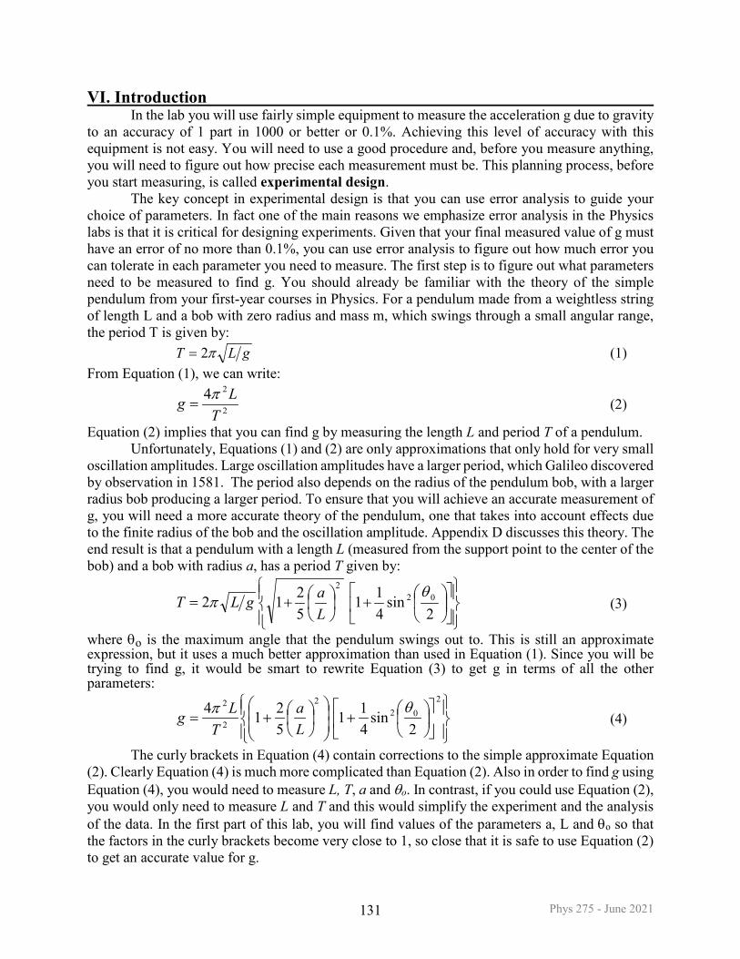
VI. Introduction In the lab you will use fairly simple equipment to measure the acceleration g due to gravity to an accuracy of 1 part in 1000 or better or 0.1%. Achieving this level of accuracy with this equipment is not easy. You will need to use a good procedure and, before you measure anything, you will need to figure out how precise each measurement must be. This planning process, before you start measuring, is called experimental design. The key concept in experimental design is that you can use error analysis to guide your choice of parameters. In fact one of the main reasons we emphasize error analysis in the Physics labs is that it is critical for designing experiments. Given that your final measured value of g must have an error of no more than 0.1%, you can use error analysis to figure out how much error you can tolerate in each parameter you need to measure. The first step is to figure out what parameters need to be measured to find g. You should already be familiar with the theory of the simple pendulum from your first-year courses in Physics. For a pendulum made from a weightless string of length L and a bob with zero radius and mass m, which swings through a small angular range, the period T is given by: gLT π2= (1) From Equation (1), we can write:

2

24T

Lg π= (2)

Equation (2) implies that you can find g by measuring the length L and period T of a pendulum. Unfortunately, Equations (1) and (2) are only approximations that only hold for very small oscillation amplitudes. Large oscillation amplitudes have a larger period, which Galileo discovered by observation in 1581. The period also depends on the radius of the pendulum bob, with a larger radius bob producing a larger period. To ensure that you will achieve an accurate measurement of g, you will need a more accurate theory of the pendulum, one that takes into account effects due to the finite radius of the bob and the oscillation amplitude. Appendix D discusses this theory. The end result is that a pendulum with a length L (measured from the support point to the center of the bob) and a bob with radius a, has a period T given by:

+

+=

2sin

411

5212 02

2 θπ

LagLT (3)

where θo is the maximum angle that the pendulum swings out to. This is still an approximate expression, but it uses a much better approximation than used in Equation (1). Since you will be trying to find g, it would be smart to rewrite Equation (3) to get g in terms of all the other parameters:

+

+=

202

2

2

2

2sin

411

5214 θπ

La

TLg (4)

The curly brackets in Equation (4) contain corrections to the simple approximate Equation (2). Clearly Equation (4) is much more complicated than Equation (2). Also in order to find g using Equation (4), you would need to measure L, T, a and θo. In contrast, if you could use Equation (2), you would only need to measure L and T and this would simplify the experiment and the analysis of the data. In the first part of this lab, you will find values of the parameters a, L and θo so that the factors in the curly brackets become very close to 1, so close that it is safe to use Equation (2) to get an accurate value for g.

Phys 275 - June 2021 132

VII. Experiment Part A: Simplifying the Procedure The Big Picture: In this part you will work out how to arrange things so that you can use the simple Equation (2) rather than the complicated Equation (4) to find g. The period of a pendulum depends on the amplitude θ0 of the pendulum’s oscillation, which leads to a somewhat complicated expression for g (see Equation 4). Notice however that the angle only enters in Equation (4) through the factor: F1 ={1+ [¼ sin2(θ0/2)]}2. If we can choose θ0 to be small enough, then F1 will be very close to 1 and we can simply ignore this factor. In this first step of the design, you are going to set things up so that F1 - 1 is less than 10-4, which is 10 times smaller than the 0.1% precision you need to achieve for g. To proceed, recall that when x is very small compared to 1, a good approximation to ( )nx+1 can be found by making a Taylor series expansion. One finds ( ) xnx n +≈+ 11 . Use this to get a simple approximate expression for F1. If you are working with a PDF use the graphics pad to write you work directly in the space below: F1 = Next rearrange this slightly to get an expression for F1-1: F1-1 = Now use the trigonometric result to rewrite your expression for F1-1 so that it is in terms of cos(θ). F1-1 = From Figure 1 it is easy to show that

2

cos( ) 1 oxL

θ = −

Substitute this into your expression for F1-1 so that it is now in terms of xo/L. F1-1 =

( ) ( ) 2/cos12sin 2 θθ −=

Figure 1. Diagram showing a simple pendulum of length L swinging through angle θ.

Phys 275 - June 2021 133

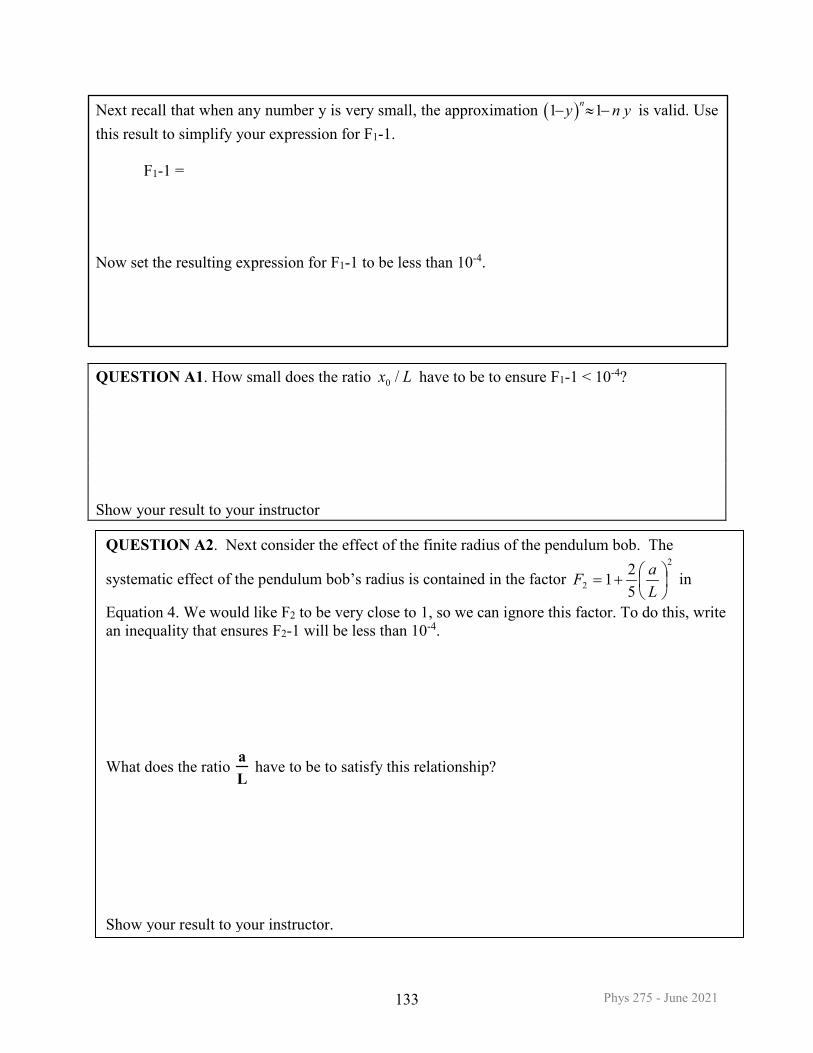
Next recall that when any number y is very small, the approximation ( )1 1ny n y− ≈ − is valid. Use this result to simplify your expression for F1-1. F1-1 = Now set the resulting expression for F1-1 to be less than 10-4. QUESTION A1. How small does the ratio Lx /0 have to be to ensure F1-1 < 10-4? Show your result to your instructor

QUESTION A2. Next consider the effect of the finite radius of the pendulum bob. The

systematic effect of the pendulum bob’s radius is contained in the factor 2

2 521

+=

LaF in

Equation 4. We would like F2 to be very close to 1, so we can ignore this factor. To do this, write an inequality that ensures F2-1 will be less than 10-4. What does the ratio a

L have to be to satisfy this relationship?

Show your result to your instructor.

Phys 275 - June 2021 134

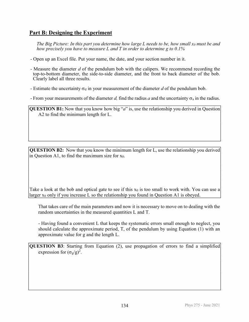
Part B: Designing the Experiment

The Big Picture: In this part you determine how large L needs to be, how small x0 must be and how precisely you have to measure L and T in order to determine g to 0.1%

- Open up an Excel file. Put your name, the date, and your section number in it. - Measure the diameter d of the pendulum bob with the calipers. We recommend recording the

top-to-bottom diameter, the side-to-side diameter, and the front to back diameter of the bob. Clearly label all three results.

- Estimate the uncertainty σd in your measurement of the diameter d of the pendulum bob. - From your measurements of the diameter d, find the radius a and the uncertainty σa in the radius.

QUESTION B1: Now that you know how big “a” is, use the relationship you derived in Question

A2 to find the minimum length for L.

QUESTION B2: Now that you know the minimum length for L, use the relationship you derived in Question A1, to find the maximum size for x0. Take a look at the bob and optical gate to see if this x0 is too small to work with. You can use a larger x0 only if you increase L so the relationship you found in Question A1 is obeyed. That takes care of the main parameters and now it is necessary to move on to dealing with the

random uncertainties in the measured quantities L and T. - Having found a convenient L that keeps the systematic errors small enough to neglect, you

should calculate the approximate period, T, of the pendulum by using Equation (1) with an approximate value for g and the length L.

QUESTION B3: Starting from Equation (2), use propagation of errors to find a simplified

expression for (σg/g)2.

Phys 275 - June 2021 135

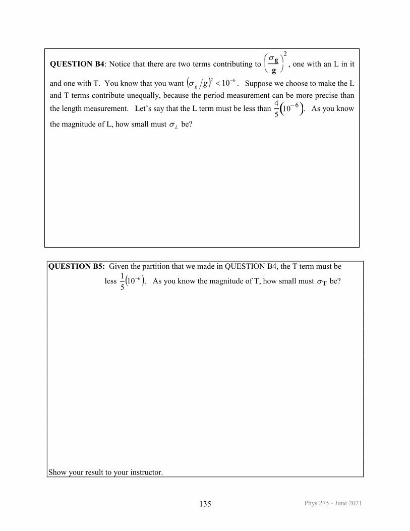
QUESTION B5: Given the partition that we made in QUESTION B4, the T term must be

less ( )61051 − . As you know the magnitude of T, how small must σT be?

Show your result to your instructor.

QUESTION B4: Notice that there are two terms contributing to σ gg

2, one with an L in it

and one with T. You know that you want ( ) 62 10−<ggσ . Suppose we choose to make the L and T terms contribute unequally, because the period measurement can be more precise than the length measurement. Let’s say that the L term must be less than 4

510− 6( ). As you know

the magnitude of L, how small must Lσ be?

Phys 275 - June 2021 136

Part C: Calibrated Measurement of the Pendulum Length The Big Picture: In this part you will make a calibrated measurement of the pendulum’s length. DO NOT START THIS PART UNTIL AFTER YOU HAVE GONE THROUGH ALL OF PARTS A and B WITH YOUR INSTRUCTOR.

- In Question B4 you found how small Lσ must be (you should have found it must be smaller than about 1.4 mm). Ordinarily we are just worried about the uncertainty σL in the measurement, but you also need the measurement to be accurate to within σL. Unfortunately, the 2-m wooden rulers that you will be using do not have the required level of accuracy. To obtain a measurement with this level of accuracy, you will need to use a ruler that is known to be accurate because it has been compared to a calibrated standard meter. The lab has two metal calibrated 2-m rulers that are known to be accurate to within about ± 0.1 mm. By comparing your 2-meter wooden ruler to one of the metal calibrated 2-m rulers you can obtain a measurement with the required accuracy and also find the inaccuracy of your 2-m wooden ruler, i.e. whether it is really 2 meters long, or is too short or too long by some factor.

- Each 2-m wooden ruler is uniquely numbered, usually in the middle of the stick. Record the

stick number in your spreadsheet. Use only this ruler for making measurements. Never use anyone else’s wooden ruler. Make sure your ruler has a sliding square stop and a pointer.

- In the next few steps you will very carefully measure the length L' from the bottom of the

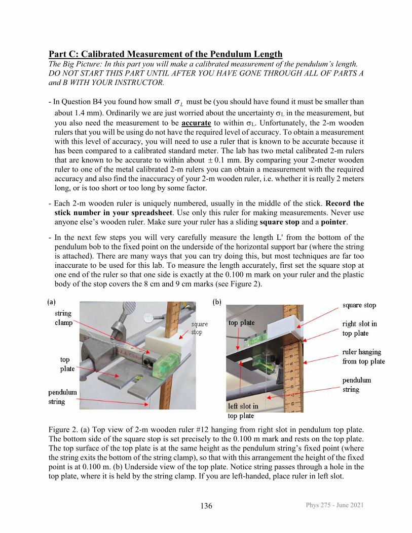
pendulum bob to the fixed point on the underside of the horizontal support bar (where the string is attached). There are many ways that you can try doing this, but most techniques are far too inaccurate to be used for this lab. To measure the length accurately, first set the square stop at one end of the ruler so that one side is exactly at the 0.100 m mark on your ruler and the plastic body of the stop covers the 8 cm and 9 cm marks (see Figure 2).

Figure 2. (a) Top view of 2-m wooden ruler #12 hanging from right slot in pendulum top plate. The bottom side of the square stop is set precisely to the 0.100 m mark and rests on the top plate. The top surface of the top plate is at the same height as the pendulum string’s fixed point (where the string exits the bottom of the string clamp), so that with this arrangement the height of the fixed point is at 0.100 m. (b) Underside view of the top plate. Notice string passes through a hole in the top plate, where it is held by the string clamp. If you are left-handed, place ruler in left slot.

Phys 275 - June 2021 137

- Place the 2-meter wooden ruler into the slot in the top plate, with the square stop holding the ruler in place on the top plate (see Figure 2). Use the slot on the right if you are right-handed and choose the left slot if you are left-handed. Note that the top surface of the top plate is at the same level as the fixed point where the pendulum string is attached. The top end of the pendulum string is now at y1=0.100 m with an uncertainty that is much less than 1 mm.

- Now slide the pointer on the wooden ruler until it is just grazing the bottom of the pendulum and

clamp it in place. With the pointer clamped in place and the pendulum swinging back and forth, verify that the bottom of the bob is just barely brushing the top of the pointer. Don’t push or pull on the ruler or the pendulum bob, just let the ruler hang and the bob swing back and forth. Adjust the pointer’s position until you are satisfied and then show your instructor.

- Remove the ruler from the top plate. Double-check that bottom side of the square stop is still at

exactly the y1 = 0.100 m mark. Next carefully determine the location y2 of the pointer. You can use your phone or web camera to take pictures of the pointer; this may be easier to read.

- Record y1, y2 and L' = y2 - y1 in your spreadsheet. This is the uncalibrated length from the fixed

point (at the top of the string) to the bottom of the bob. - Being very careful not to bump the square stop or pointer, move your ruler to the table at the

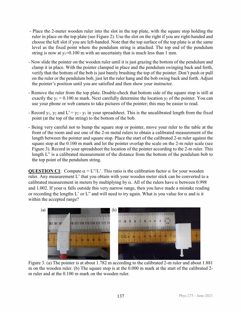
front of the room and use one of the 2-m metal rulers to obtain a calibrated measurement of the length between the pointer and square stop. Place the start of the calibrated 2-m ruler against the square stop at the 0.100 m mark and let the pointer overlap the scale on the 2-m ruler scale (see Figure 3). Record in your spreadsheet the location of the pointer according to the 2-m ruler. This length L” is a calibrated measurement of the distance from the bottom of the pendulum bob to the top point of the pendulum string.

QUESTION C1: Compute α = L”/L’. This ratio is the calibration factor α for your wooden ruler. Any measurement L’ that you obtain with your wooden meter stick can be converted to a calibrated measurement in meters by multiplying by α. All of the rulers have α between 0.998 and 1.002. If your α falls outside this very narrow range, then you have made a mistake reading or recording the lengths L’ or L” and will need to try again. What is you value for α and is it within the accepted range?

Figure 3. (a) The pointer is at about 1.782 m according to the calibrated 2-m ruler and about 1.881 m on the wooden ruler. (b) The square stop is at the 0.000 m mark at the start of the calibrated 2-m ruler and at the 0.100 m mark on the wooden ruler.

Phys 275 - June 2021 138

- Have another student measure the length L” of your setup using their ruler. While they are doing this, you should measure their setup using your ruler. You must use your ruler to measure their apparatus, and they must use their ruler to measure your apparatus. At this point, don’t confer with your partner or let them know what you obtained for your L” or their L”. The idea is that you want to make sure they finish getting a good independent measurement of your L”, without being biased by your result, and vice versa. This will give each of you a check on how accurately you might be measuring L”. Carefully record and label the L” for your partner’s apparatus in your spreadsheet.

- After you and your partner get values for L" for each of your setups, your instructor should insist

that you record them on the whiteboard at the front of the lab. It can be confusing where to write your values for each L”, so consult with your instructor!

- If two measurements of L" for the same apparatus differ by more than σL (see your answer to question B4), then one or both of you have made an error that is too large. You must sort this out with the other person. This can take up to an hour, but it is critical to get the length pinned down accurately. Do not proceed past this point until you have resolved the disagreement…. this is not a case where you can “agree to disagree” unless your disagreement is less than σL. If you are off by 1 cm or more, it is likely that one or both of you have misread the ruler, for example by looking at the wrong side of the pointer. If you disagree by a few mm, use both rulers to measure one setup and then try laying both rulers side by side on the floor to see if the pointers are physically agreeing on the length.

- Once the agreement with your partner is acceptable, use your value for L" and d to calculate the

length L of the pendulum using " / 2L L d= − .

- Find the uncertainty σL in the length L of the pendulum by using the following simple result from propagating the errors

2 2 2

2 2 2" "" 4

dL L d L

L LL d

σσ σ σ σ∂ ∂ = + = + ∂ ∂

Here σL” is the uncertainty in the length L” reported by the 2-m ruler. Considering the inaccuracy in the length (a systematic error of ± 0.1 mm) and the intrinsic precision of readings made with a ruler that is read to the nearest 1-mm interval ( ± 0.28 mm, see Appendix A), we can take:

2 2" (0.0001 ) (0.00028 ) 0.0003L m m mσ = + =

Note: We gave the inaccuracy of the calibrated metal 2-m rulers as ± 0.1 mm, but how can we

know this is correct? Only by comparing the ruler to a better standard of length. The Phys 275 Lab also has a 1-m standard ruler (see Figure 4) that has a known length of L1= 1.00000 m ±5x10-5 m at 20 oC. Since it is only 1-m long, and is not marked every mm, it is hard to use for calibrating the 2-m wooden rulers. Never the less, it can be used to check the 2-m rulers if needed.

Figure 4. Photo of 1-m standard of length. The length is 1.00000 m ± 0.00005 m at 20 oC.

Phys 275 - June 2021 139

Part D: Measure the Pendulum Period In this part you will use an optical gate to find the period T of the pendulum by measuring

the times at which the pendulum's string crosses through the optical gate. When the string passes through the optical gate, there will be a minimum in transmitted light intensity, causing the voltage from the sensor to dip. If you set the optical gate sampling rate at a frequency of fsample, then the time between samples is δt=1/fsample. Ideally, the minimum intensity occurs at some time tm, where m is the sample number. However, two successive times tm and tm+1 may both reach the minimum value (see Figure 5), leading to large uncertainty in the crossing time. For this reason, it is better to define the crossing time as the time when the intensity is changing rapidly and passing through a specific “threshold” value. In Figure 4, the dashed horizontal line shows a threshold value of 2.000V. To find the crossing time, you can simply choose the time tn when the voltage is closest to 2.000 V and decreasing. In this case tn = 0.394 s. With this measurement scheme, you can think of the time sampling as being equivalent to having a “time-ruler” that is marked in intervals of δt. The 1/3 rule then gives the uncertainty: σt = δt/3 = 1/(3fsample). (5) Equation 5 gives the uncertainty in the time when a particular crossing occurred. But what you will need is the uncertainty in the measured time interval TN = tN - to for N periods. From propagation of errors, this uncertainty is just:

220 tNtTN

σσσ += , (6) where σt0 is the uncertainty in the time of the intensity minimum at the beginning of the first period, when N = 0, and σtN is the uncertainty in the time of the minimum intensity at the end of the N-th period. These two uncertainties are equal and given by Equation 5. Substituting gives

sample

ttNtT fN 322 2

022

0 ==+= σσσσ (7)

The average time for a single period is given by:

NTT N

av = (8)

Figure 5. Plot of intensity versus time t as the string crosses through the optical gate. Dashed line shows the choice of a 2V threshold and the identification of the crossing time at tn. The minimum occurs somewhere between times tm and tm+1.

Phys 275 - June 2021 140

QUESTION D1: Propagate errors to find the uncertainty in Tav as a function of σNT and N: (Hint: Is there any uncertainty in N?) Use Equation 7 to substitute for

NTσ and get σTav as a function of f and N. Show your result to your instructor. The string crosses the optical gate in about tc ≈ 15 ms. You need to get several samples taken during this time interval. This means that fsample must be very much larger than 1/tc, i.e.

csample tf /1>> . Calculate 1/tc and then select a sampling frequency fsample that is very much bigger than this value. Do not exceed 1000 Hz (Hint: Does 1000 exceed 1000)! QUESTION D2: What must N be to get σT to meet the condition set in question B5? - Turn on the power to the optical gate and check that the gate is placed so the string cuts through

the gate at the bottom of the swing.

- Set the sampling rate in LoggerPro according to your answer to question D3. - Pull the pendulum bob aside a small distance (see you answer to QUESTION B2). Roughly

measure x0 and record it in your spreadsheet (you won't need it very accurately). Then let the bob start swinging.

- Use Logger Pro to get a data set. Copy the data into your spreadsheet and make a plot (as in

Figure 5). Note that a full period corresponds to two crossings, one where the bob is heading forward through the gate and the other where it is coming back through the gate.

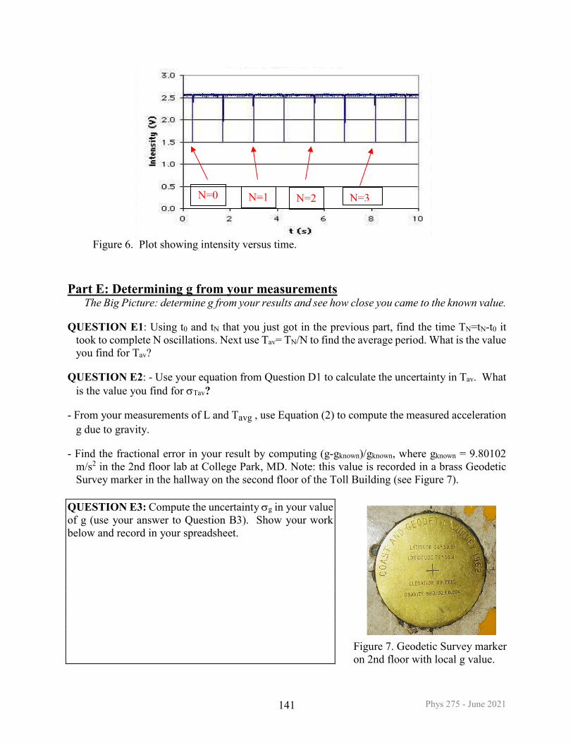
- Carefully examine your plot of intensity versus time and count how many complete oscillations

N there are (there will be two dips for each oscillation, see Figure 6). Record in your spreadsheet. - Now find the time t0 when the string first passes through the optical gate and the one time tN that

the pendulum completes oscillation number N (see Figure 6). You need very accurate numbers. Hint: choose a threshold voltage and discuss with your instructor. Record t0 and tN in your spreadsheet.

Phys 275 - June 2021 141

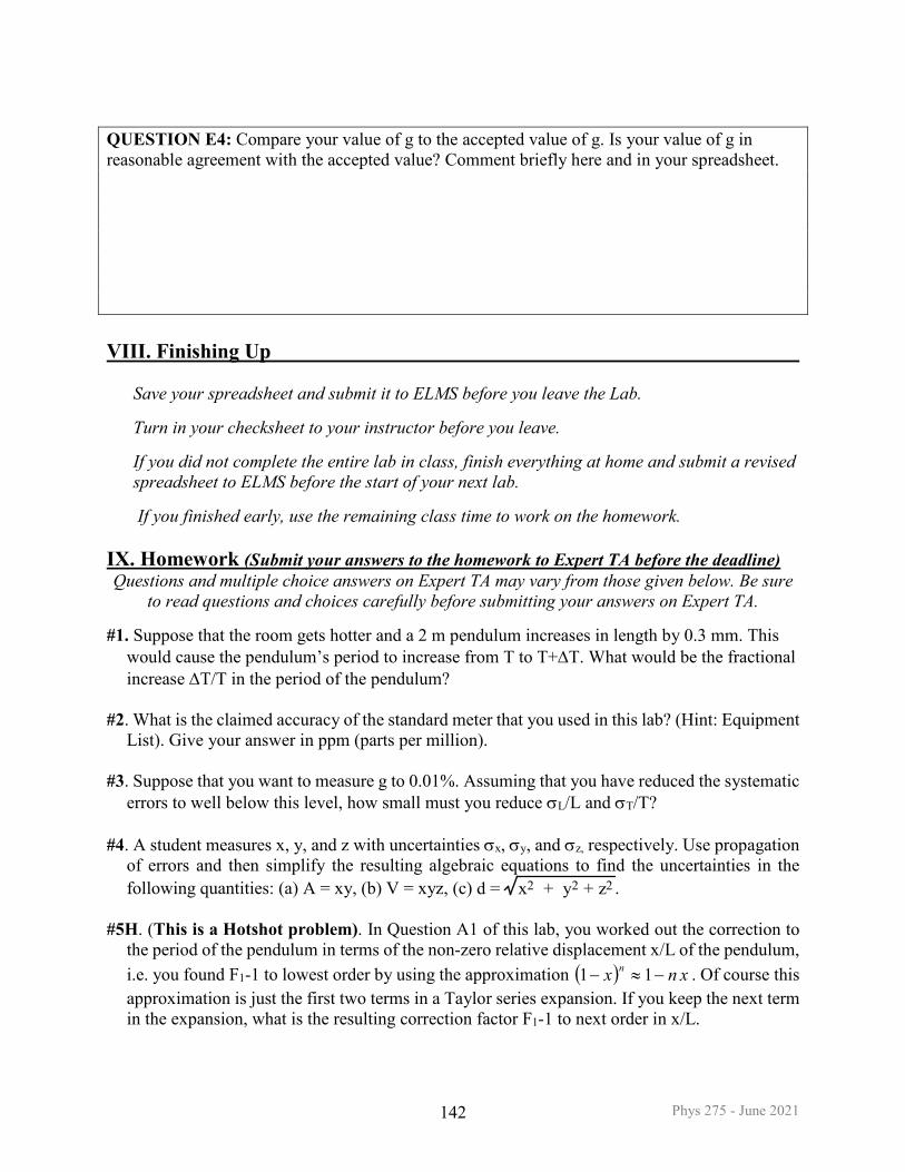
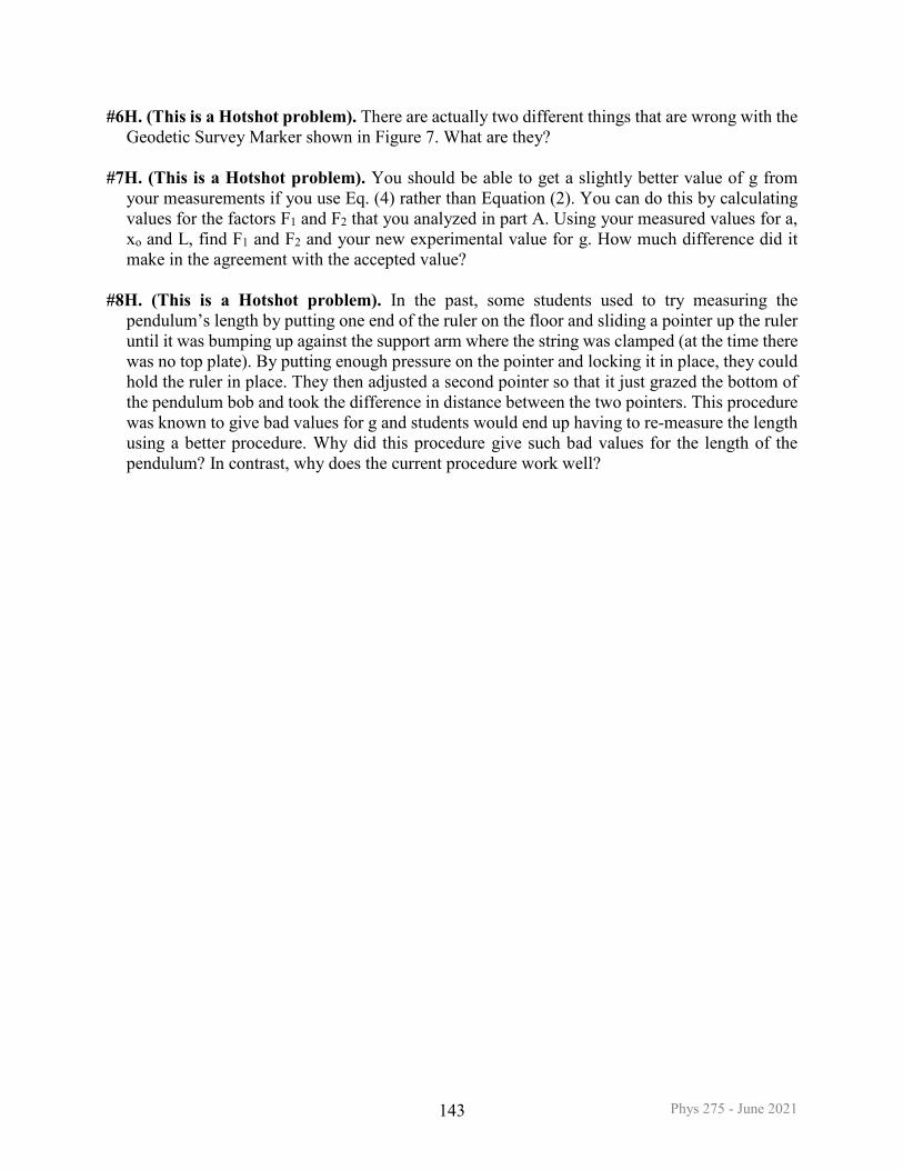
Figure 7. Geodetic Survey marker on 2nd floor with local g value.

Figure 6. Plot showing intensity versus time.

Part E: Determining g from your measurements

The Big Picture: determine g from your results and see how close you came to the known value. QUESTION E1: Using t0 and tN that you just got in the previous part, find the time TN=tN-t0 it

took to complete N oscillations. Next use Tav= TN/N to find the average period. What is the value you find for Tav?

QUESTION E2: - Use your equation from Question D1 to calculate the uncertainty in Tav. What

is the value you find for σTav? - From your measurements of L and Tavg , use Equation (2) to compute the measured acceleration

g due to gravity. - Find the fractional error in your result by computing (g-gknown)/gknown, where gknown = 9.80102

m/s2 in the 2nd floor lab at College Park, MD. Note: this value is recorded in a brass Geodetic Survey marker in the hallway on the second floor of the Toll Building (see Figure 7).

QUESTION E3: Compute the uncertainty σg in your value of g (use your answer to Question B3). Show your work below and record in your spreadsheet.

N=0 N=3 N=1 N=2

Phys 275 - June 2021 142

QUESTION E4: Compare your value of g to the accepted value of g. Is your value of g in reasonable agreement with the accepted value? Comment briefly here and in your spreadsheet. VIII. Finishing Up

Save your spreadsheet and submit it to ELMS before you leave the Lab. Turn in your checksheet to your instructor before you leave. If you did not complete the entire lab in class, finish everything at home and submit a revised spreadsheet to ELMS before the start of your next lab. If you finished early, use the remaining class time to work on the homework.

IX. Homework (Submit your answers to the homework to Expert TA before the deadline) Questions and multiple choice answers on Expert TA may vary from those given below. Be sure

to read questions and choices carefully before submitting your answers on Expert TA.

#1. Suppose that the room gets hotter and a 2 m pendulum increases in length by 0.3 mm. This would cause the pendulum’s period to increase from T to T+∆T. What would be the fractional increase ∆T/T in the period of the pendulum?

#2. What is the claimed accuracy of the standard meter that you used in this lab? (Hint: Equipment

List). Give your answer in ppm (parts per million). #3. Suppose that you want to measure g to 0.01%. Assuming that you have reduced the systematic

errors to well below this level, how small must you reduce σL/L and σT/T? #4. A student measures x, y, and z with uncertainties σx, σy, and σz, respectively. Use propagation

of errors and then simplify the resulting algebraic equations to find the uncertainties in the following quantities: (a) A = xy, (b) V = xyz, (c) .

#5H. (This is a Hotshot problem). In Question A1 of this lab, you worked out the correction to

the period of the pendulum in terms of the non-zero relative displacement x/L of the pendulum, i.e. you found F1-1 to lowest order by using the approximation ( ) xnx n −≈− 11 . Of course this approximation is just the first two terms in a Taylor series expansion. If you keep the next term in the expansion, what is the resulting correction factor F1-1 to next order in x/L.

d = x2 + y2 + z2

Phys 275 - June 2021 143

#6H. (This is a Hotshot problem). There are actually two different things that are wrong with the Geodetic Survey Marker shown in Figure 7. What are they?

#7H. (This is a Hotshot problem). You should be able to get a slightly better value of g from

your measurements if you use Eq. (4) rather than Equation (2). You can do this by calculating values for the factors F1 and F2 that you analyzed in part A. Using your measured values for a, xo and L, find F1 and F2 and your new experimental value for g. How much difference did it make in the agreement with the accepted value?

#8H. (This is a Hotshot problem). In the past, some students used to try measuring the

pendulum’s length by putting one end of the ruler on the floor and sliding a pointer up the ruler until it was bumping up against the support arm where the string was clamped (at the time there was no top plate). By putting enough pressure on the pointer and locking it in place, they could hold the ruler in place. They then adjusted a second pointer so that it just grazed the bottom of the pendulum bob and took the difference in distance between the two pointers. This procedure was known to give bad values for g and students would end up having to re-measure the length using a better procedure. Why did this procedure give such bad values for the length of the pendulum? In contrast, why does the current procedure work well?