Experiment Design Using ARM Software

Steven R. Gylling, Ph.D.

Gylling Data Management, Inc.

Plan Experiments to Have:

A reasonable chance of distinguishing anticipated treatment differences

The optimum number of replicates required to meet objectives

An efficient experimental design and randomization for desired precision

Cost-effective utilization of the available experimental area

January 2015 2

Why is Planning Critical?

Can reduce costs by selecting optimum number of replicates and samples

Expected treatment differences are typically < 10%, and frequently < 5%, so small precision gains can help to:

Distinguish an actual treatment difference (reject null hypothesis H0)

Strengthen evidence of no treatment diff.) (do not reject null hypothesis H0)

January 2015 3

ARM 2015 Power and Efficiency Planner

January 2015 4

Power and Efficiency Planner

"Lock at" to keep 3-4 columns constant

Calculates table of possible values for "unlocked" columns (e.g. Rep or CV)

Values entered by protocol writer are carried into trials created from protocol, conveying protocol expectations to trialist

January 2015 5

Power and Efficiency Planner

Plan replicates to achieve required precision 5 treatments with CV=5, 10% mean diff.

January 2015 6

Summary

Reps αSL=Significance

7 1% 0.01

5 5% 0.05

4 10-15% 0.1-0.15

3 20-30% 0.2-0.3

2 40-50% 0.4-0.5

Power and Efficiency Planner

CV effect on minimum detectable % mean difference at 5% αSL for 10 treatments, 4 reps

January 2015 7

Detectable Difference between Trt. Means

CV % Mean Diff.

3 6.17% difference

4 8.2% difference

5 10.3% difference

6 12.3% difference

7 14.4% difference

Randomization Quality Review

Goal is to improve experiment precision:

1. Arrange replicates as squares, not strips

2. Equalize treatment distribution

a. Balance average distance from all other treatments

b. Balance “Edge effect” across treatments

3. Randomize all replicates

January 2015 8

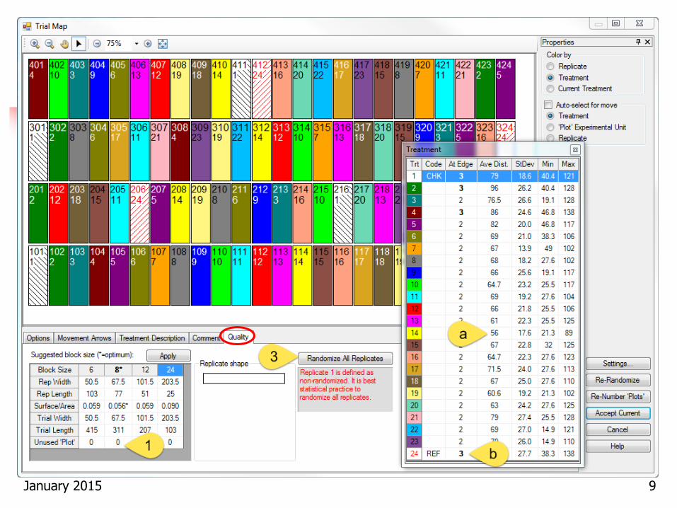
Randomization Quality Tab

January 2015 9

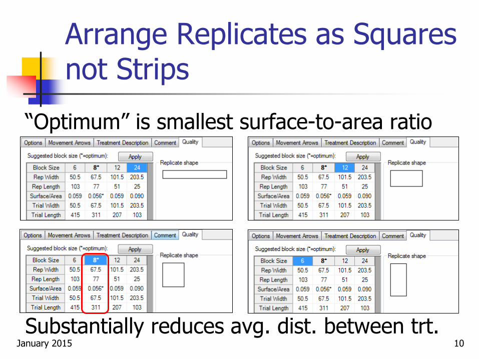
Arrange Replicates as Squares not Strips

“Optimum” is smallest surface-to-area ratio

Substantially reduces avg. dist. between trt.

January 2015 10

Equalize Treatment Distribution

“Undesirable” layout of 7 treatments and 5 replicates in Randomized Complete Block:

Trt. 6 in middle 3 columns of all reps

Trt. 5 in right 2 cols for all but one plot

Example from Federer, “Experimental Design” 1955 January 2015 11

Uses “Average Distance of Treatment” Comparison (ADTC)

van Es and van Es, “Spatial Nature of Randomization and Its Effect on the Outcome of Field Experiments”, Agron J, 85:420-428 (1993).

Goal is to create spatially-balanced designs.

Comparison between treatments 1 and 2 is taken from 5 plots for each treatment.

Measure the plot-to-plot distance for each plot containing treatment 1 to the paired plot within replicate containing treatment 2, for a total of 5 distances.

ADTC for treatment pair 1-2 is average of the 5 distances.

Repeat this comparison for all treatment pairs. January 2015 12

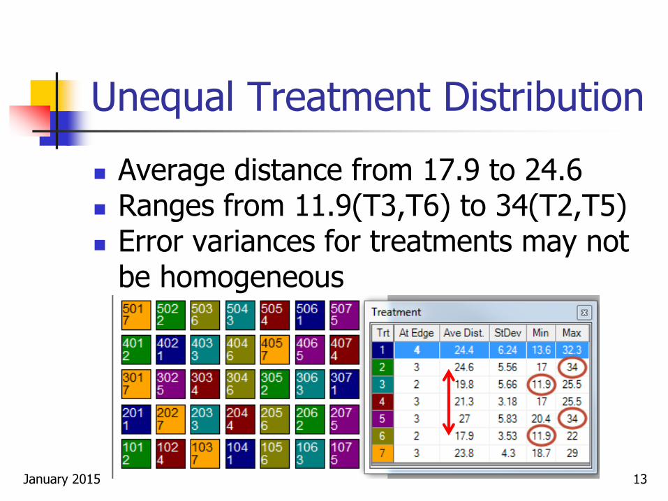
Unequal Treatment Distribution

Average distance from 17.9 to 24.6 Ranges from 11.9(T3,T6) to 34(T2,T5) Error variances for treatments may not

be homogeneous

January 2015 13

Unbalanced “Edge effect”

Treatment 1 occurs at edge 4 times, T2 and T3 at edge only 2 times

January 2015 14

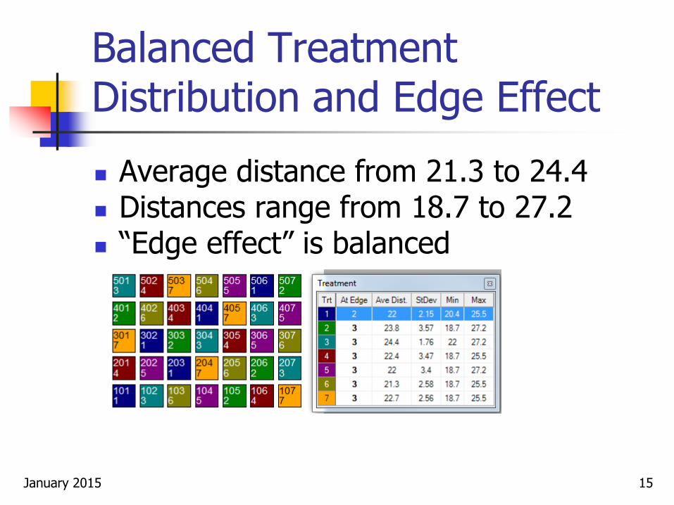
Balanced Treatment Distribution and Edge Effect

Average distance from 21.3 to 24.4 Distances range from 18.7 to 27.2 “Edge effect” is balanced

January 2015 15

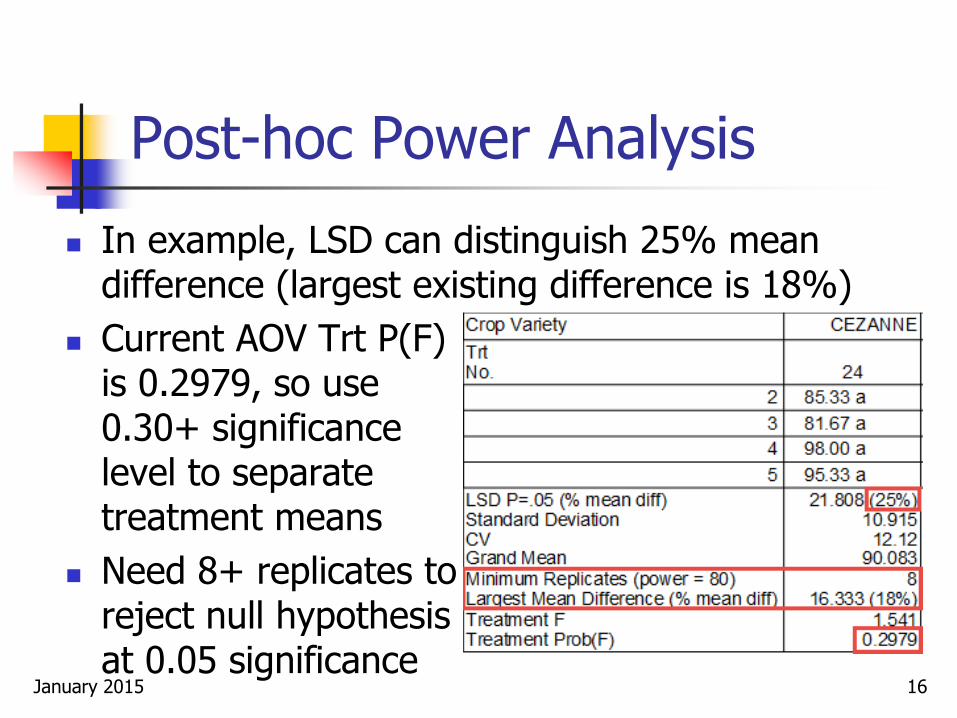
Post-hoc Power Analysis

In example, LSD can distinguish 25% mean difference (largest existing difference is 18%)

Current AOV Trt P(F) is 0.2979, so use 0.30+ significance level to separate treatment means

Need 8+ replicates to reject null hypothesis at 0.05 significance

January 2015 16

Summary

Software tools can help improve trial quality and efficiency:

Plan appropriate number of replicates

Improve quality of randomizations

Analyze results to improve planning of follow-up experiments

January 2015 17