expected utility theory - rice universityecon501/lectures/decision_eu.pdf · expected utility...

Expected Utility Theory

Simon GrantRice University

Timothy Van ZandtINSEAD

22 November 2007

This is a chapter for the forthcoming Handbook of Rational and Social Choice,Paul Anand, Prasanta Pattanaik, and Clemens Puppe, eds., Oxford UniversityPress, 2008. We review classic normative expected utility theory. Our goal isto frame the subsequent chapters (which consider more modern extensions toand deviations from this classic theory) in a way that is accessible to the non-specialist but also useful to the specialist. We start from scratch with a revealedpreference approach to the existence of a utility function. We then present themathematical structure of additive and linear utility representations and their ax-iomatizations, in the context of abstract choice theory and using intertemporalchoice as a source of examples. We are thus able to focus on this mathematicalstructure without the interference of the specific interpretation and notation fordecision under uncertainty. Furthermore, this approach allows us to focus on theinterpretation of the axioms when we turn to decision under uncertainty.

Contents

1. Introduction 1

2. Descriptive, prescriptive, and normative theories 2

3. A review of choice, preferences, and utility 3

4. Hidden assumption: Consequentialism 3

5. Weak axiom of revealed preference 4

6. From preferences to choice rules 6

7. Infinite choice sets and continuity assumptions 7

8. Additive utility 8

9. Linear preferences 12

10. Cardinal uniformity across factors 15

11. States of nature and acts 20

12. Sure-thing principle and additivity 22

13. Lotteries 27

14. Subjective expected utility without objective probabilities 31

15. Subjective expected utility with objective probabilities 33

16. Conclusion 36

References 40

Acknowledgments: We are deeply indebted to Peter Wakker for providing detailed comments on twoearlier drafts and helping shape this chapter. We also benefited from the feedback of Paul Anand andClemens Puppe, from discussions with Enrico Diecidue, and from corrections by Philippe Delquiéand Alminas Zaldokas.

Email addresses: [email protected] (Grant); [email protected] (Van Zandt).

Grant and Van Zandt • Expected Utility Theory 1

1. Introduction

This handbook is a modern look at decision theory and social choice. It empha-sizes recent developments that go beyond the classic theory of utility and expectedutility. However, a sensible starting point is the classical theory, a benchmark thatwill frame departures considered in subsequent chapters. Furthermore, it remainsthe prominent workhorse for applied economics.

This chapter presents the main features of that classical theory. The topicis broad and has been treated so much elsewhere that we do not attempt to betechnically comprehensive. Instead, we opt for a succinct and pedagogical treat-ment that will be accessible to nonspecialists yet still useful to the specialist forframing the subsequent chapters.

The theory reviewed here has had a long and complicated development. Ex-pected utility dates back at least to Bernoulli (1738). As a resolution to the famousSt. Petersburg paradox, he used a logarithmic utility index defined over wealthto compute a finite price for a gamble with an unbounded expected value. Eventhe modern foundations are a half-century old, with the development of an ax-iomatic choice-theoretic foundation for expected utility occurring roughly fromthe mid-1920s to the early 1960s.

We neither structure the chapter around such historical development nor at-tempt to explain it; a proper treatment would be too lengthy and would distractfrom the content of this chapter, whereas a succinct treatment would have toomany unfair omissions. Instead, our goal is to clarify the interpretation and math-ematical role of the various axioms that form the theory. We have the benefit ofhindsight and of our freedom to deviate from the chronology of the theory’s de-velopment.

Rather than delve immediately into choice under uncertainty, we start fromscratch with basic preference theory (Sections 2–7). Not all of this volume relatesto decision under uncertainty, but our other motive for reviewing this theory is toemphasize the assumptions that are already implicit when one represents choicesover uncertain prospects by a complete and transitive preference relation.

The fundamental mathematical properties of expected utility representationsare additivity and linearity. Our main expository innovation is to remain in thegeneral choice setting a little longer (Sections 8–10) in order to explore the in-dependence assumptions that lead to such structure without reference to decisionunder uncertainty. We can thereby (a) clarify the mathematics without the bag-gage of the uncertainty framework and (b) discuss the axioms in other contexts,such as multi-attribute decision problems and intertemporal choice, so that theirsignificance in decision under uncertainty is then better understood.

We thus do not reach decision under uncertainty until the middle of the chap-ter. We first introduce the “states of the world” (Savage) framework for represent-ing uncertainty in Section 11. This precedes our treatment of the lotteries rep-resentation of objective uncertainty (Section 13), in a reversal of the usual (andhistorical) order, because the states framework is useful and intuitive whether un-certainty is subjective or objective and because we refer to it when interpreting theaxioms of the lotteries model. Overall, we proceed as follows. After presentingthe states framework in Section 11, we take our characterization of preferences


and utility as far as an independence axiom and state-dependent expected utilityin Section 12. We then turn to expected utility for lotteries (objective uncertainty)in Section 13. In Sections 14 and 15, we return to the full subjective expectedutility representation in the states model with state-independent utility.

As noted, we emphasize the link between the independence axioms in con-sumer theory, in expected utility for objective lotteries, and in expected utilityunder subjective uncertainty. Fishburn and Wakker (1995) provide a comprehen-sive study of how these different versions arose and evolved historically. The wayin which we motivate the axioms—as following from dynamic consistency andconsequentialism—is analogous to the treatment in Hammond (1988).

Our decision to study additive and linear utility before any applications todecision under uncertainty has the advantages we claimed above. It comes attwo costs. First, those familiar with expected utility theory may be disconcertedto see, in the first half of the chapter, familiar axioms and theorems with onlypassing references to the seminal work in expected utility theory from whichthey originated. However, such omissions are rectified in the second half of thechapter and, with this warning, the reader should suffer no ill consequences. Thesecond cost is that we have to invent “context-free” names for several old axiomsfrom expected utility theory.

2. Descriptive, prescriptive, and normative theories

Decision theory has two goals: To describe how agents do make decisions (de-scriptive decision theory) and to prescribe how agents should make decisions(prescriptive decision theory). As in any theoretical modeling, decision theorybalances accuracy and simplicity. A prescriptive decision theory that is too com-plicated to learn or implement is hardly useful for a decision maker. A descriptivetheory should be simple because it is meant to be a framework that organizes andunifies a variety of situations and behavior, because it should be tractable enoughto derive conclusions, and because we may need to estimate the parameters ofthe theory from a limited amount of data.

A third branch of decision theory, normative decision theory, tries to describehow a hypothetical, infinitely intelligent being would make decisions. This maysound speculative and impractical but it provides important foundations for de-scriptive and prescriptive theories. A normative theory is inherently simpler thanan overtly descriptive or prescriptive theory because it need not concern itselfwith such complications as (a) errors or forgetting and (b) the heterogeneity ofthe intelligence and experience of decision makers. There are only a few ways tobe perfect, but many ways to be imperfect!

Simplicity is good, but how does a normative theory serve the goals of de-scriptive or prescriptive theory? Humans are goal oriented and work hard topursue these goals. Any descriptive theory should capture this first-order con-sideration, and a normative model is a powerful and parsimonious way to do so.To develop a prescriptive theory that helps mortal humans (with all their limita-tions) make decisions, it is useful to understand how unboundedly rational beingswould make decisions.


This chapter develops classical rational choice theory, particularly expectedutility theory, as a normative model. We leave it to subsequent chapters to eval-uate how well it serves as a descriptive or prescriptive theory.

3. A review of choice, preferences, and utility

Before tackling decision making under uncertainty, we study the theory of choicewithout uncertainty. Let’s call our decision maker “Anna”.

In most of this chapter, we limit attention to static choice. This means weconsider a single decision that Anna makes. We thus suppress the fact that Annamay anticipate having to make choices in the future and that current decisionsare intertwined with such future decisions. However, we do not thereby suppresstime: the objects of choice could be time paths of consumption.

We ignore much of the information processing that Anna must do in order tomake a decision. The only input to Anna’s problem is the set of possible alter-natives, which we allow to vary. There is a fixed set X containing all potentialalternatives, and Anna is presented with a set A ⊂ X from which she must choose,called a choice set. For example, X is the set of all consumption bundles and Ais the budget set, which depends on prices and the agent’s wealth. Alternatively,X could be the set of potential presidential candidates and A the set of candidateson the ballot. We want a model of what Anna would choose from each set offeasible alternatives.

Assume that X is finite and that every nonempty subset A of X is a potentialfeasible set. For each set A ⊂ X of feasible alternatives, let C(A) be the elementsof A that Anna might choose from A. She must always choose something, whichmeans that C(A) is nonempty, but C(A) may contain more than one item becauseof indifference. Call C(·) her choice rule. Our game is to find some conditionsthat lead to a simple representation of choice. The representation should allowone to derive qualitative conclusions in models without knowing specific choicesand should have few parameters, all of which could be estimated empirically.

There are two complementary approaches. One is to start with a choice ruleas a primitive. From this “empirical” object, one derives (revealed) preferences.The other approach is to start with preferences as the primitive. From these, onederives the choice rule. We follow the first (revealed preference) approach.

4. Hidden assumption: Consequentialism

We will be as explicit as space permits about hidden assumptions. For exam-ple, we have already outlined the static nature of the model. Another hiddenassumption is consequentialism: Anna cares about consequences—not how con-sequences are achieved.

In the decision model we have developed so far, “consequences” refers to thealternatives and “consequentialism” means that Anna does not care how she endsup facing a particular choice set A ⊂ X or how she chooses from A. For example,in consumer theory, one might suppose that Anna cares only about consumption


and not about the prices that determine which consumption bundles are afford-able. In decision making under uncertainty, we may suppose that Anna cares onlyabout probabilities of different outcomes and not about how these probabilitiesare generated (e.g., about whether uncertainty is resolved in one step or insteadin a multi-stage lottery).

We can redefine consequences in order to circumvent any particular violationof consequentialism. If Anna cares about prices, then we define a consequencenot only by how much she consumes of different goods but also by the pricesshe faces (we have thus redefined the set X). If Anna cares about the stages atwhich uncertainty unfolds, then a consequence can be defined to include suchinformation.

However, if we proceed this way without constraint, then—in our abstractmodel—a consequence would be defined by not only the element of X that Annaends up with but also by the set A from which she was able to select it. Hence,there would be no link or consistency conditions between the choices Anna mightmake from A ⊂ X and those she might make from A′ ⊂ X . We would have avacuous theory. Instead, we must be able to define consequences in a sufficientlyrestrictive way that we can envision Anna being presented with different sets ofconsequences and caring only about those consequences, not about how thosesets were generated.

From the empirical side of the theory, there is another hidden assumption.We are supposedly studying a single decision that Anna makes. However, forthat decision she will end up facing a single choice set A ⊂ X . We will neverbe able to observe an inconsistency between C(A) and C(A′) unless one of thefollowing two conditions is satisfied.

1. When presented with different hypothetical choice sets, Anna can report thechoices she would make.

2. Anna faces different instances of this problem at different times, and how shechooses from any choice set does not vary from one instance to the other.

Thus, we assume that one of these two conditions holds.

5. Weak axiom of revealed preference

Let x and y belong to X . Then x is revealed weakly preferred to y if x ∈ C(A) forsome A ⊂ X containing x and y (i.e., if y is available but x may be chosen). If alsoy /∈ C(A) then we say that x is revealed preferred to y or, if we want to emphasizethat the preference is not weak, that x is revealed strictly preferred to y.

The weak axiom of revealed preference (WARP) states that if x is revealedweakly preferred to y, then y is not revealed preferred to x. This is defined ex-plicitly in Axiom 1.

Axiom 1 (WARP). Let x and y belong to X , and let A and B be subsets of Xcontaining x and y. If x ∈ C(A) and y ∈ C(B), then x ∈ C(B).

WARP is a natural axiom of a normative theory, but it is at best an approx-


imation for descriptive or prescriptive theories. Especially when choice sets arelarge and complex, achieving such consistency is difficult.

This one consistency condition gets us far. First, it implies that the choicerule can be summarized by or deduced from more limited information: the binarychoices or preferences. To make this statement more precise, we first define, forx, y ∈ X ,

x � y if x ∈ C({x, y}) (x is weakly preferred to y);x � y if x � y but not y � x (x is (strictly) preferred to y);x ∼ y if x � y and y � x (x is indifferent to y).

The binary relations �, �, and ∼ are called the (weak) preference, strict prefer-ence, and indifference relations, respectively.

Definition 1. Let � be the preference relation defined for a choice rule C(·) asin the previous paragraph. Then the choice rule satisfies preference maximizationif, for every A ⊂ X and x ∈ A,

x ∈ C(A) ⇐⇒ x � y ∀y ∈ A.

In words, choices from large sets are consistent with binary choices. If we knowAnna’s binary choices (preferences), then we can derive C(·). Preference maxi-mization implies a considerable savings in the amount of information required inorder to know C(·).

It is also useful for Anna’s preferences to satisfy some consistency conditionsthemselves.

Definition 2. A binary relation � is a weak order if it satisfies the followingconditions.

1. (Completeness) For all x, y ∈ X , we have x � y or y � x (or both).2. (Transitivity) For all x, y, z ∈ X , if x � y and y � z then x � z.

Completeness of the preference relation follows from the assumption thatC has nonempty values. Transitivity is the important consistency condition; itfollows from WARP.

Proposition 1. The choice rule C(·) satisfies WARP if and only if (a) itsatisfies preference maximization and (b) the preference relation is complete andtransitive.

Proof. Samuelson (1938) defined WARP in the context of consumer theory (bud-get sets) and single-valued demand. Arrow (1959) defined WARP (as we did) forgeneral choice rules—that is, for abstract choice sets and possibly multi-valuedchoices. Proposition 1 is implied by Theorems 2 and 3 in Arrow (1959). �

One advantage of complete and transitive preferences is that they can be rep-resented by a utility function.


Definition 3. Let � be a preference relation on X and let U : X → R be afunction. Then U is a utility representation of �, and � is represented by theutility function U , if for all x, y,∈ X we have

x � y ⇐⇒ U (x) ≥ U (y).

Proposition 2. A preference relation � on X is complete and transitive if andonly if it has a utility representation.

Proof. The utility representation is easily constructed recursively. See Birkhoff(1948, Thm. 1, p. 31) for such a proof for countable X . �

Thus, WARP also means that Anna makes choices as if she maximized autility function, as stated in the next corollary.

Corollary 1. The choice rule C(·) satisfies WARP if and only if there is a utilityfunction U : X → R such that

C(A) = arg maxx∈A

U (x)

for all A ⊂ X.

If U : X → R is a utility representation of a preference relation � on X andif f : R → R is any strictly increasing function, then f ◦ U : X → R is also arepresentation of �. (The composition f ◦U is called a monotone transformationof U ). Therefore, the magnitudes of the utility values of a representation haveno particular meaning—they only define the ordinal relationship �.

6. From preferences to choice rules

Suppose instead that we let Anna’s preference relation � be the primitive andthen derive choices from this relation. (The primitive is thus any binary relationon X , which attains meaning as a preference relation through the subsequent usemade of it in the model.) In this approach, preference maximization becomes anaxiom that defines the choice rule: For A ⊂ X ,

C(A) = {x ∈ A | x � y ∀y ∈ A} .

Given this axiom, the standard way to proceed is by assuming that preferences arecomplete and transitive and then concluding that (a) the choice rule C(·) satisfiesWARP and (b) preferences have a utility representation.

We highlight the axiom of preference maximization—that choices from largesets be consistent with binary choices—because it is a critical consistency con-dition. If one observed a violation of WARP or a violation of transitivity, then itwould be reasonable to doubt preference maximization. Retaining it and merelytweaking the axioms on preferences could be a poor way to develop a theory thatencompasses such empirical violations.


7. Infinite choice sets and continuity assumptions

Infinite choice sets require two modifications to the theories described so far. Onesuch modification is that the choice rule might not be defined on all subsets of X :it has a restricted domain. For example, if X = R+ represents monetary prizes andif Anna would always choose the higher of two monetary prizes, then preferencemaximization would imply that Anna’s choice from all of X or from [0, 1) is notwell-defined.

This should be viewed as a nonsubstantive technical restriction. In practice, itis fair to say that Anna would always make a decision. (Not announcing a choicealso represents a decision, since there must be some default outcome that occurs.)The kind of choice sets that are suppressed from the domain of C typically eitherare unrealistic (“you can have as much money as you want”), arise only becausean inherently discrete problem has been modeled as a continuous approximation(“you can have any amount of money in [0, 1)”), or would lead to well-definedchoices if certain aspects of the problem were fully modeled (e.g., if the time ittook to get finer and finer divisions of a good were taken into account).

The second modification of the theory, which may be needed only if thechoice set is uncountable, is that there may be an important role for some kind ofcontinuity assumption on the preference relation.

Definition 4. Let X be endowed with a topology. A preference relation � onX is continuous if {y ∈ X | y � x} and {y ∈ X | x � y} are closed for all x ∈ X .

One representation theorem on infinite choice sets is the following.

Theorem 1. Suppose that X is a separable metric space and that � is contin-uous, complete, and transitive. Then � has a continuous utility representation.

Proof. See Theorem II in Debreu (1954). The actual topological assumption ismore general: that the topology on X have a countable base. For a metric space,this assumption is equivalent to separability. See Debreu (1964) for a discussionand alternate proofs of variants on this result. �

In Theorem 1, the continuity assumption is needed in order to obtain anyutility representation at all, but it has the added benefit that the theorem shows theexistence of a continuous representation. In the approach that starts at preferencesand derives choices, continuity assumptions are used to ensure that choices arewell-defined at least on compact sets. Continuity of the representation may beimportant in further applications.

However, it would be surprising if continuity of preferences were requiredfor the mere existence of a (not necessarily continuous) utility representation. Infact, there are nontopological variants of Theorem 1 (and of many other theoremsin this chapter) that use an “order-theoretic” or “algebraic” approach. We presentone example.

Define a subset Z of (X , �) (or of any weakly-ordered space) to be order-dense in (X , �) if, for all x, y ∈ X such that x � y, there exists z ∈ Z such that


x � z � y. For any Y ⊂ R, the linearly-ordered space (Y,≥) has a countableorder-dense subset. One can think of a utility representation as embedding theordered space (X , �) into (R,≥). Therefore, (X , �) must also have a countableorder-dense subset. This necessary condition is also sufficient for the existenceof a utility representation.

Theorem 2. If � is complete and transitive and contains a countable order-dense subset, then � has a utility representation.

Proof. This is Lemma II in Debreu (1954). It is closely related to results for lin-ear orders by Cantor (1895) and Birkhoff (1948, Thm. 2, p. 32). (See a completeproof of Birkhoff’s theorem in Krantz et al. (1971, Thm. 2.2).) One proves Theo-rem 2 by studying the induced linear order over equivalence classes of (X , �) andthereby reducing it to the case of linear orders. This is made explicit in Theorem3.1 of Fishburn (1970).

We provide a warning to the reader. The term “order dense” has several sim-ilar definitions in the mathematics and mathematical economics literature. Forexample, for a linearly-ordered space (Y,≥), Birkhoff (1948) defines Z ⊂ Y tobe order dense in (Y,≥) if, for all x, y ∈ Y \Z such that x > y, there is z ∈ Z suchthat x > z > y. This definition is equivalent to ours for a linearly-ordered set butnot for a weakly-ordered set. �

Theorems 1 and 2 are linked by the following fact: If X is a separable metricspace and � is continuous, then (X , �) has a countable order-dense subset.

An example of preferences that have no countable order-dense subset andhence have no utility representation are lexicographic preferences onR2

+: (x1, x2) �(y1, y2) if and only if either x1 > y1 or x1 = y1 and y1 > y2. Any order-densesubset of (R2

+, �) is not countable because it must contain an element for everyvalue of the first coordinate.

Apart from this brief aside, we stick to the topological approach throughoutthis chapter. The topological assumptions tend to be both easier to state and morefamiliar to the reader than are the algebraic assumptions. The interested readermay consult Krantz et al. (1971) and Fishburn (1970) for further development ofthe algebraic approach.

8. Additive utility

Maintained assumptions. The rest of this chapter is about the additional struc-ture that preferences and their utility representation may have. Therefore, as weproceed and even as the set of alternatives varies, we avoid repetition by main-taining the assumptions that choices satisfy preference maximization, that thesymbol � denotes the preferences relation, and that � is complete and transitive.


8.1. Overview

We study two types of structure that one might impose on preferences or utility:additivity and linearity. Why do we tackle these technical topics in the settingof abstract choice theory when this chapter is supposed to focus on choice underuncertainty? In decision under uncertainty, additivity is the most important struc-ture imposed on preferences over state-contingent outcomes, and linearity is themost important assumption imposed on preferences over lotteries. We would liketo understand the mathematics of these structures in the absence of a particularinterpretation so that (a) the mathematical structure is clearer, (b) when we reachdecision under uncertainty, we can focus on their interpretation rather than themath, and (c) we can better understand the relationship between expected utilitytheory and, say, intertemporal choice.

8.2. Additive separability

In this section, we assume that X is a product set: X = X1 × · · · × XJ . Eachcomponent j = 1, . . . , J is called a factor. Here are some possible cases.

1. There are J goods; (x1, . . . , xJ ) ∈ X is a consumption bundle; and Xj = R+

is the set of possible quantities of any one of the goods.2. There is one good with multiple varieties, which are characterized by J at-

tributes; a particular variety is given by a list (x1, . . . , xJ ) ∈ X of attributes;and Xj is the set of possible values of attribute j.

3. There are J periods; (x1, . . . , xJ ) ∈ X is a time path of consumption; and Xj

is the set of possible consumption bundles in period j.4. There are J states of nature; (x1, . . . , xJ ) ∈ X is a state-contingent outcome;

and Xj is the set of possible outcomes in state j.5. There are J people; (x1, . . . , xJ) ∈ X is an allocation; and Xj is the set of

possible consumption bundles of agent j. (The decision maker is an outsideobserver.)

Given preferences � on X , we are interested in whether there is a represen-tation of the form

U (x1, . . . , xJ ) =J

∑j=1

uj(x j)

for some functions uj : Xj → R. Such a representation is called additive or addi-tively separable.

Suppose such a representation exists. Recall that any monotone transforma-tion of U represents the same preferences. However, it need not be additive. Thefamily of additive representations can be fairly narrow. Under a variety of as-sumptions, including those of Theorem 3 to follow, an additive representation isunique up to an affine transformation. That is, V is another additive representa-tion if and only if V = a+ bU , where a ∈ R and b ∈ R++. The magnitudes of theutilities of the different factors have some meaning because they are aggregatedacross factors to determine the overall ranking of alternatives.

For example, suppose x1, x2, x3, x4 ∈ X , with x1 � x2 and x3 � x4. Comparethe “extra kick” from getting x1 rather than x2 with the extra kick of getting x3


rather than x4 and measure this comparison by the ratio

U (x1) −U (x2)

U (x3) −U (x4). (1)

This ratio is the same for any additive representation U , yet can have any positivevalue if we allow for nonadditive representations.

For this reason, additive utilities are often referred to as cardinal utilities.However, only ratios such as (1) are uniform across additive representations.Thus, additive utilities are not interpersonal cardinal scales as used in utilitari-anism.

8.3. Joint independence

An immediate consequence of an additive representation is that preferences sat-isfy joint independence, meaning that “how one ranks what happens with somefactors does not depend on what happens with the other factors”.

We introduce some notation to formalize joint independence. For a given setK ⊂ {1, . . . , J} of factors, let XK ≡ ∏ j∈K Xj. For a partition {K, L} of {1, . . . , J},we may write an element of X as (a, c), where a ∈ XK denotes the values for thefactors in K and c ∈ XL denotes the values for the factors in L. For the specialcase in which K is a singleton { j}, we may write (x j, x− j), where x j ∈ Xj andx− j ∈ X− j ≡ ∏k �= j Xk.

Axiom 2 (Joint independence). For all partitions {K, L} of {1, . . . , J}, for alla, b ∈ XK , and for all c, d ∈ XL,

(a, c) � (b, c) ⇐⇒ (a, d) � (b, d).

Joint independence (a term used by Krantz et al. 1971, p. 339) has also beencalled conjoint independence, strong separability (Strotz 1959), independenceamong factors (Fishburn 1970, Sec. 4.1; Debreu 1960), and coordinate indepen-dence (Wakker 1989). It was called the sure-thing principle by Savage (1954) fora model in which the factors are states.

We mentioned intertemporal choice as a setting in which one may want towork with additive representations. Note how strong the joint independence con-dition can be in that setting. It implies that how Anna prefers to allocate con-sumption between periods 2 and 3 does not depend on how much she consumedin period 1. However, after a shopping and eating binge on Tuesday, Anna mightwell prefer to take it easy on Wednesday and defer some consumption until Thurs-day. Joint independence also implies that Anna’s ranking of today’s meal optionsdoes not depend on what she ate yesterday and that whether she wants to talk toher boyfriend today does not depend on whether they had a fight yesterday.

Yet additive utility is a mainstay of intertemporal models in economics. Theassumption becomes a better approximation when outcomes are measured at amore aggregate level, as is typical in such models. Suppose, then, that the modeldoes not include such details as meal options and social relationships, address-ing instead one-dimensional aggregate consumption. Then joint independence


in a two-period model is satisfied as long as Anna’s preferences are monotone(though we will see that, in this case, the assumption is not enough to guaranteean additive utility representation). With more than two time periods, joint inde-pendence implies that Anna’s desired allocation between periods 2 and 3 doesnot depend on period-1 consumption; this assumption is more plausible when aperiod is one year rather than one day.

8.4. A representation theorem

Joint independence is the main substantive assumption needed to obtain an addi-tive representation. Here is one such representation theorem.

Theorem 3. Assume J ≥ 3 and that the following hold.

1. Xj is connected for all j = 1, . . . , J.2. � is continuous.3. � satisfies joint independence.4. Each factor is essential: for all j, there exist x j, x′j ∈ Xj and x− j ∈ X− j such

that (x j, x− j) � (x′j, x− j).

Then � has an additive representation that is continuous.

Proof. This result is similar to Debreu (1960, Thm. 3), except that the latteralso assumes that each Xj is separable. Krantz et al. (1971, Thm. 13, Sec. 6.11)provides an algebraic approach to such a representation; the topological assump-tions are replaced by algebraic conditions on the preferences and the continu-ity of the additive representation is not derived. Their Theorem 14 then showsthat our topological assumptions imply their algebraic conditions. Wakker (1988,Thm 4.1) complements this by showing that, under the topological assumptions,any additive representation must be continuous. �

8.5. Revealed trade-offs

Joint independence should not be confused with the weaker assumption of single-factor independence (also called weak separability): that preferences over eachsingle factor do not depend on what is held fixed for the other factors. The factthat such independence must hold for preferences over multiple factors is thereason for the term “joint” in “joint independence”.

For example, any monotone preference relation on RJ+ satisfies single-factor

independence. Yet even with the additional assumptions of Theorem 3, not allmonotone preferences have additive representations. To illustrate this, we needonly find a continuous and monotone function that cannot be transformed mono-tonically into an additive function; U (x1, x2) = min{2x1 + x2, x1 + 2x2} will do.

With just two factors, single-factor and joint independence are the same. Thisis why Theorem 3 assumed that there were at least three essential factors. To han-dle the two-factor case, one needs an assumption that is more explicit about thetrade-offs Anna may make between factors. We now review such an axiomatiza-tion and its extension to J factors.


Let j ∈ {1, . . . , J}, let aj, bj , c j, dj ∈ Xj, and let x− j, y− j ∈ X− j. Suppose

(x− j, aj) � (y− j, bj) but (x− j, c j) � (y− j, dj).

This reveals (one might say) that, keeping fixed the comparison x− j versus y− j onfactors other than j, the strength of preference for c j over dj on factor j weaklyexceeds the strength of preference for aj over bj on factor j. For nonadditiveutility, a switch in such revealed strength of preference could easily occur. Thatis, there might also be w− j, z− j ∈ X− j such that

(w− j, aj) � (z− j, bj) but (w− j, c j) ≺ (z− j, dj).

If there is such a reversal then coordinate j reveals contradictory trade-offs.The assumption that no coordinate reveals contradictory trade-offs is also calledtriple cancellation for the case of J = 2 (Krantz et al. 1971) and generalizedtriple cancellation for J ≥ 2 (Wakker 1989).

One way to put the “no contradictory trade-offs” condition into words isroughly as follows. When it holds, Anna could say—

When I choose among consumption paths for the week, one of my considerationis what I will do on Friday night. I prefer to go to a great movie on Friday ratherthan read a book. I also prefer to go to a dance rather than play poker. But thefirst comparison is more likely to swing may decision than the second one.

—without any qualification about what is happening the rest of the week.Our next theorem derives an additive representation from this condition.

Theorem 4. Assume J ≥ 2 and that the following hold:

1. Xj is a connected for all j = 1, . . . , J;2. � is continuous;3. no coordinate reveals contradictory trade-offs.

Then � has an additive representation that is continuous.

Proof. See Krantz et al. (1971, Sec. 6.2) for the two-factor case. See Wakker(1989, Thm. III.6.6) for the J-factor case. �

9. Linear preferences

9.1. Linear utility

Suppose that X is a convex subset of Rn. Then a subclass of utility functions thatare additive across dimensions of the space are those that are linear.

Let u ∈ Rn be the vector representation of the linear utility function. Thatis, U (x) = ∑n

i=1 uixi = u · x, where u · x denotes the inner product. A typicalindifference curve is

{x ∈ X | u · x = u}.


That is, the indifference curves are parallel hyperplanes (more specifically, theintersection of such parallel hyperplanes with X), and there is a direction U—perpendicular to the hyperplanes—that points in the direction of increasing util-ity.

These two conditions are also sufficient for the existence of a linear utility rep-resentation. We merely take the normal vector of one of the hyperplanes, pointingin the direction of increasing utility, and this defines a linear utility representation.

9.2. Linearity axiom

What axioms on the preference relation give us linear and parallel indifferencecurves? Let’s start with just the linearity of a particular indifference curve. Roughlyspeaking, we need that, for any two points on an indifference curve, any linepassing through those points also lies on the indifference curve—at least whereit intersects X . We can state this condition as follows.

Axiom L1. For all 0 < α < 1 and all x, y ∈ X ,

αx + (1 − α)y ∼ x ⇐⇒ x ∼ y. (2)

Because Axiom L1 is an “if and only if” condition, it is stronger than convex-ity of the indifference curves and really does imply that they are linear subspaces.Take x and y on the same indifference curve and let z ∈ X be any point on theline through x and y. If z lies between x and y, then we must have z ∼ x becauseof the ⇐ direction of condition (2). If instead z lies beyond y, then y is a con-vex combination of x and z and we have z ∼ x because of the ⇒ direction ofcondition (2).

The second condition we want is for the translation of an indifference curveto be another indifference curve, so that the indifference curves are parallel. Wemight state this as follows.

Axiom L2. For all x, y ∈ X and z ∈ Rn such that x + z ∈ X and y + z ∈ X ,

x + z ∼ y + z ⇐⇒ x ∼ y.

However, there is a more succinct way to combine Axioms L1 and L2.

Axiom L3. For all 0 < α < 1 and all x, y, z ∈ X ,

αx + (1 − α)z ∼ αy + (1 − α)z ⇐⇒ x ∼ y. (3)

Axioms L1 and L2 are equivalent to Axiom L3. By letting z = y in condi-tion (3), one obtains condition (2). Figure 1 illustrates Axiom L3 for z that is notcolinear with x and y. The axiom then implies that x ∼ y if and only if x′ ∼ y′

and x′′ ∼ y′′. One can see why this axiom implies that the indifference curves areparallel.

However, Axiom L3 does not ensure that there is a common direction of in-creasing utility. To add this property, we can strengthen L3 by stating it in termsof � rather than ∼. We thus obtain the final statement of the linearity axiom.


�

�

�

�

� �

�

x y

z

x′

x′′

y′

y′′

Figure 1. An illustration of Axiom L3 or Axiom L: Axiom L3 states that x ∼ y if and only if x′ ∼ y′

and x′′ ∼ y′′; Axiom L is the same but for �.

Axiom L (Linearity). For all 0 < α < 1 and all x, y, z ∈ X ,

αx + (1 − α)z � αy + (1 − α)z ⇐⇒ x � y.

9.3. Continuity and the representation theorem

We have controlled for everything but the dimensionality of the indifference curves.It is fine for X to be one huge indifference curve; we can use the trivially linearutility function that maps all of X to 0. Otherwise, we need the dimensionality ofthe indifference curves to be one less than the dimensionality of X , so that eachcurve is the intersection of X and a hyperplane.

For example, lexicographic preferences on R2 satisfy the linearity axiom, andeach indifference curve is indeed a linear subspace: a point. However, lexico-graphic preferences do not have a linear utility representation because the di-mensionality of the indifference curves is too small.

A continuity assumption suffices to get the dimensionality correct. Consider,for example, an indifference curve through an alternative x that is neither thebest nor the worst element of X . If preferences are continuous, then the set ofpoints worse than x is open and the set of points better than x is open; hence theirunion cannot be a connected set. This means that the indifference curve throughx must separate these two sets, which in turn requires that the indifference curve’sdimension be one less than the dimension of X .

Given the linearity axiom, continuity is guaranteed by the following Archimedeanaxiom (which would be weaker than continuity in the absence of linearity).

Axiom 3 (Archimedean). For all x, y, z ∈ X , if x � y � z then there exist α, Β in(0, 1) such that

αx + (1 − α)z � y � Βx + (1 − Β)z.

We now have our representation theorem.

Theorem 5. If � satisfies the linearity and Archimedean axioms, then � has alinear utility representation.


Proof. As we will see in Sections 13, this proposition is similar to the expectedutility theorem of von Neumann and Morgenstern (1944). However, this form isdue to Jensen (1967, Thm. 8). It can be generalized to infinite-dimensional vectorspaces. The simplest way is to develop a theory for an abstract generalizationof convex sets, called “mixture spaces”, as in Herstein and Milnor (1953). Acomprehensive treatment can be found in Fishburn (1970, Chaps. 8 and 10). �

9.4. Linearity implies joint independence

Suppose there are J factors and each Xj is a convex subset of Euclidean space.Then X = X1×· · ·×XJ is also a convex set. According to Theorem 5, if � satisfiesthe linearity and Archimedean axioms, then � has a linear utility representation,which can be written

U (x1, . . . , xJ ) =J

∑j=1

uj · x j.

Since such a representation is additive across factors, � satisfies joint indepen-dence. Thus, with such a factor structure, a corollary to Theorem 5 is that thelinearity and Archimedean axioms imply joint independence.

However, the Archimedean axiom is not needed for this implication. A di-rect proof of the stronger result, stated in the next proposition, clarifies the linkbetween linearity and joint independence.

Proposition 3. If � satisfies linearity then � satisfies joint independence.

Proof. Let {K, L} be a partition of {1, . . . , J}, let a, b ∈ XK , and let c, d ∈ XL.Assume (a, c) � (b, c). We show that (a, d) � (b, d).

Linearity and (a, c) � (b, c) imply

12 (a, c) + 1

2 (a, d) � 12 (b, c) + 1

2 (a, d). (4)

By simple algebra, we can swap the terms a and b on the right hand side of (4),so that this equation becomes

12 (a, c) + 1

2 (a, d) � 12 (a, c) + 1

2 (b, d). (5)

Since (a, c) is a common term on both sides of the preference in (5), we obtainfrom a second application of linearity that (a, d) � (b, d). �

10. Cardinal uniformity across factors

10.1. Ordinal versus cardinal uniformity

Return to the setting of Section 8, in which there are J factors and X = X1 ×· · ·×XJ . There we found conditions under which Anna’s preferences would have anadditive representation

U (x1, . . . , xJ ) =J

∑j=1

uj(x j).


Suppose that each factor has the same set of possible alternatives: Xj = X for j =1, . . . , J. It is then meaningful to consider the special case in which preferencesover each factor are the same—i.e., in which uj and uk represent the same ordinalpreferences for j �= k.

To state this condition in terms of preferences rather than utility, define thepreference relation on factor 1 (for example) as follows. Pick x−1 ∈ ∏J

j=2 Xj andthen define x1 �1 x′1 by (x1, x−1) � (x′1, x−1); single-factor independence impliesthat this preference ordering on X1 is the same no matter which x−1 we use todefine it. Then the preferences � satisfy ordinal uniformity across factors if � j

is the same for all j.However, ordinal uniformity adds little tractability beyond that of a general

additive representation. It would be more interesting that the within-factor utilityfunctions uj were mere positive affine transformations of each other. Then wecould find a common utility function u : X → R and weights Δ1, . . . , ΔJ > 0 suchthat

U (x1, . . . , xJ ) =J

∑j=1

Δ ju(x j).

Such a representation has cardinal uniformity across factors.For example, suppose that the factors are different time periods. Then such a

representation is what we mean by time-independent preferences with discount-ing. We might normalize the factors by dividing by Δ1; then the new Δ1 equals 1and we interpret Δ j as the discount factor from period j to period 1.

Such time independence of the utility representation simplifies economic mod-els and allows one to derive stronger results. What is the essence of cardinaluniformity that allows for this? We can separate the relative importance ofthe factors from the within-factor preferences. The weights {Δ1, . . . , ΔJ} pro-vide a meaningful measure of the importance of the factors. For example, ina multi-agent intertemporal general equilibrium model, the assumption that allconsumers have the same discount factors (i.e., the same impatience) is a pow-erful restriction even if their within-period utility functions u are heterogeneous.Without time-independent preferences, we would not even be able to formulatesuch as assumption.

Ordinal uniformity of preferences does not imply cardinal uniformity of theutility representation. Cardinal uniformity requires additional restrictions, whichwe explore in the rest of this section.

10.2. Ranking of factors

As the preceding intertemporal consumption example illustrates, one of the keyfeatures of cardinal uniformity is that there is a measure {Δ1, . . . , ΔJ} of the rel-ative importance of the different factors. In terms of preferences, we can definean ordinal version of this condition as follows.

Axiom 4 (Joint ranking of factors). Suppose that preferences satisfy ordinaluniformity and let �∗ be the common-across-factors ordering on X . Let x1, x2, x3, x4 ∈X be such that x1 �∗ x2 and x3 �∗ x4. Let K, L ⊂ {1, . . . , J} and let, for example,


x1K be the element of XK that equals x1 on each coordinate. Then

(x1K , x2

Kc ) � (x1L , x2

Lc ) ⇐⇒ (x3K , x4

Kc ) � (x3L, x4

Lc ). (6)

Joint ranking of factors is the same as Savage’s P4 axiom, which we will seein Section 11. It yields an unambiguous weak order over the subsets of factorswhen we interpret (x1

K , x2Kc ) � (x1

L, x2Lc ) in equation (6) as meaning that the set of

factors K is more important than the set of factors L.Ordinal uniformity across factors has no implications for the trade-offs across

factors, whereas joint ranking of factors does. For example, consider an intertem-poral consumption example with a single good and monotone preferences. Ordi-nal uniformity holds merely because preferences are monotone. Joint ranking offactors implies additional restrictions, such as the following.

1. If Anna prefers the consumption path (100, 98, 98) over the consumptionpath (98, 100, 98), then she must also prefer (40, 30, 30) over (30, 40, 30).This captures the idea that Anna is impatient—not a normative assumptionbut one that is, at least, easy to interpret and empirically motivated.

2. The word “joint” (in “joint ranking of factors”) applies because K and L canbe arbitrary subsets of factors. Thus, suppose that Anna prefers the con-sumption path (100, 98, 98, 100, 98) over (98, 100, 100, 98, 98), which re-flects fairly complicated trade-offs between the periods. Then she must alsoprefer (40, 30, 30, 40, 30) over (30, 40, 40, 30, 30). This goes well beyondimpatience.

However, joint ranking of factors (with also joint independence and ordinaluniformity) is not yet sufficient for the existence of a cardinally uniform repre-sentation unless the choice set is rich enough for the axioms to impose enoughrestrictions. The problem is analogous to the way joint independence is sufficientfor an additive representation when there are three factors but not when there areonly two. We explore three ways to resolve this problem.

10.3. Enriching the set of factors

One approach is to enrich the set of factors so that it is infinite and perfectlydivisible.

The first steps are to extend the definition of an additive representation to aninfinite set of factors and then extend Theorem 3 to axiomatize the existence ofsuch a representation. For this we refer the reader to Wakker and Zank (1999,Thm. 12). Joint independence remains the main behavioral assumption for addi-tivity. Some additional technical assumptions are needed to handle the nonatomic-ity of the set of factors.

For example, suppose the set of factors is an interval [0, 1] of time. A con-sumption path is a function x : [0, 1] → X . Joint independence and additionaltechnical assumptions might yield an additive representation of the form

U (x) =∫ 1

0u(x( j), j) d j;


here, for each j, u(·, j) : X → R is the within-factor utility for factor j. In thisexample, integration is with respect to the Lebesgue measure, so (a) any set offactors of Lebesgue measure 0 is negligible, in the sense that changing a con-sumption plan on such a set does not change utility, and (b) the set of factorsis nonatomic. Such features hold generally in the representation of Wakker andZank (1999) and are important for what follows. Absent nonatomicity, the set offactors may not be rich enough for joint ranking of factors to imply cardinal uni-formity. However, we repeat that these are essentially restrictions on the settingand not on the behavior of the decision maker.

We now show that, in this example, joint ranking of factors is sufficient to gofrom an additive representation to one that is also cardinally uniform. To keepthe illustration simple, we assume that X contains only the three elements a, b, c.The main step is the following lemma.

Lemma 1. Assume ordinal uniformity and joint ranking of factors, and assumethat a �∗ b �∗ c. Then the ratio

u(b, j) − u(c, j)u(a, j) − u(c, j)

(7)

is the same for a.e. j.

Before proving this lemma, observe that it allows us to obtain a cardinallyuniform representation. Define v(a) = 1 and v(c) = 0, and let v(b) be the com-mon value of the ratio (7). Define also Π( j) = u(a, j) − u(c, j). Then

V (x) ≡∫ 1

0Π( j) v(x( j)) d j

equals U − ∫10 u(c, j) d j. Thus, V is an additive representation with cardinal uni-

formity.

Proof of Lemma 1. We prove a contrapositive: Given ordinal uniformity and anadditive representation, if the ratio (7) is not the same for almost every j thenjoint ranking of factors does not hold.

Suppose (7) varies on a set of positive measure. Then there exist Ρ > 0 anddisjoint sets K, L ⊂ [0, 1] such that

u(b, j) − u(c, j)u(a, j) − u(c, j)

> Ρ for j ∈ K andu(b, j) − u(c, j)u(a, j) − u(c, j)

< Ρ for j ∈ L. (8)

Given nonatomicity, we can find A ⊂ K and B ⊂ L of strictly positive measuresuch that ∫

A(u(a, j) − u(c, j)) d j =

∫B(u(a, j) − u(c, j)) d j. (9)

Let x1 be equal to a on A and to c elsewhere; let x2 be equal to a on B and celsewhere. Observe that

U (x1) −U (x2) =∫

A(u(a, j) − u(c, j)) d j −

∫B(u(a, j) − u(c, j) d j = 0. (10)


That is, x1 ∼ x2.Joint ranking of factors implies that this same indifference should hold if y1

and y2 are defined accordingly except with a replaced by b. However, the twoinequalities ∫

A(u(b, j) − u(c, j)) d j > Ρ

∫A

(u(a, j) − u(c, j)) d j,

∫B(u(b, j) − u(c, j)) d j < Ρ

∫B

(u(a, j) − u(c, j)) d j

(which following from the two inequalities in equation (8)), together with equal-ity (9), imply that∫

A(u(b, j) − u(c, j)) d j >

∫B(u(b, j) − u(c, j)) d j.

Therefore, as an analog to equation (10), we have U (y1) > U (y2). Hence, jointranking of factors does not hold. �

10.4. A factor-independent version of no contradictory trade-offs

The second approach is to assume that X is connected and then use, as a startingpoint, the axiom that no coordinate reveals contradictory trade-offs. We capturestate-independence by modifying the axiom so that it holds even when we per-mute the indices. That is, if

(x− j, a) � (y− j, b) but (x− j, c) � (y− j, d),

then it cannot be the case that

(w−k, a) � (z−k, b) but (w−k, c) ≺ (z−k, d).

(We are being loose in the notation: the idea is that a, b, c, d show up in coordinatej in the first equation but in coordinate k in the second equation.) The resultingaxiom is called cardinal coordinate independence or no contradictory trade-offsin Wakker (1989).

Proposition 4 (Wakker 1989). Suppose that X is connected and that allfactors are essential. Assume � is continuous and satisfies cardinal coordinateindependence. Then � has a continuous additive representation that is cardinallyuniform across factors.

Cardinal coordinate independence subsumes joint independence, ordinal uni-formity across factors, and joint ranking of factors. It captures the idea that therelative strength of trade-offs is uniform across factors.

10.5. The linear case

The third approach is to consider linear preferences. Suppose that X is a con-vex subset of Euclidean space and that we obtain an additive representation in


which each uj is linear. Recall that, if u1 and u2 (for example) are two linearrepresentations of the same ordinal preferences on X , then u2 is a positive affinetransformation of u1. Thus, linearity combined with the ordinal uniformity acrossfactors gives us cardinal uniformity across factors!

We summarize this in a single representation theorem. If X is convex, thenX = X J is also convex and so we can impose the linearity and Archimedean ax-ioms directly on �. Linearity implies additivity; the axiom of joint independenceis thus redundant. We merely need to add ordinal uniformity.

Proposition 5. Suppose � satisfies the linearity, Archimedean, and ordinaluniformity across factors axioms. Then � has a utility representation of the form

U (x1, . . . , xJ ) =J

∑j=1

Δ ju(x j),

where u : X → R is linear and continuous.

Proof. This is a consequence of Theorem 5 and the observation that ordinal uni-formity implies cardinal uniformity for a linear representation. In Section 15,we will see that this is the expected utility theorem of Anscombe and Aumann(1963). �

11. States of nature and acts

We now reach (finally!) decisions under uncertainty. The first question is basic:How do we model uncertainty? We start with the states-of-the-world formulationand then move to the more reduced-form lotteries formulation.

11.1. Setup

In a static decision problem under uncertainty, Anna is uncertain about the out-comes of her actions. A formal model should make a careful distinction betweenthose aspects of the world:

1. that she controls, which we call an action and denote by a ∈ A;2. that she is uncertain about and cannot influence, which we call a state and

denote by s ∈ S;3. that she cares directly about, which we call an outcome and denote by z ∈ Z.

These aspects are linked by a function F : A × S → Z that summarizes how theoutcome is determined by her actions (which she controls) and the state (whichshe cannot influence).

11.2. From large to small worlds

Savage (1954, p. 9) describes a state of the world as “a description of the world,leaving no relevant aspect undescribed”, but in Chapter 5 he goes on to explain


that an actual model of decisions (whether constructed by a decision theorist orcontemplated by Anna) could not contain such detail. He then draws the follow-ing link between the abstract “large worlds”, whose specification can omit nodetails, and the “small worlds” that appear in our models.

Let S∗ be the set of “large worlds” or states as envisioned by Savage. A subsetE ⊂ S∗ is called an event. To construct a model of a particular decision problem,we replace S∗ by a partition {E1, . . . , En} of S∗ that is

• fine enough that, for every action, states in the same event lead to the sameoutcome,

• but otherwise as coarse as possible.

Each state s j in the model corresponds to an event E j in the partition.Consider, for example, a portfolio choice problem in which Anna will in-

vest a fixed amount of money in securities, hold the securities for one year, andthen cash out the securities. The actions are the different portfolios Anna couldchoose. Suppose that Anna cares only about the monetary payoff of her portfo-lio; such payoffs are the outcomes. Then a state could represent the values of allthe securities at the time Anna cashes in her portfolio. Each “state” in the modelis really an event. For instance, distinct large-world states within an event coulddiffer in terms of the outcome of elections, the growth of the plants in Anna’sgarden, and other factors that do not affect portfolio returns.

11.3. From actions to acts

The decision maker chooses an action a ∈ A. For example, Anna chooses aportfolio. Given action a, each state s leads to outcome F(a, s). This defines amap s �→ F (a, s) from S to Z. We call such a map an act. The act s �→ F (a, s) isthe one induced by the action a.

A first assumption is that, when choosing among actions, Anna comparesthe acts that they induce. This is plausible as long as we have defined outcomescarefully enough that they include any aspects of the action that Anna may careabout (see Section 4). This leads to a reduced-form model in which Anna choosesamong acts. Let’s go a step further. Assume that Anna can contemplate hypo-thetical choices among any acts, even those that are not induced by any action.

(Our distinction between actions and acts abuses vocabulary but is useful.When Savage coined the term “act”, he was thinking of it as synonymous with“action”. However, he jumped immediately to the reduced form and defined anact to be a mapping between S and Z. It is useful to retain the notion of the trueaction that Anna controls so that the model can more naturally describe actualdecision problems.)

We can relate the resulting model to the ones developed earlier in the chapteras follows.

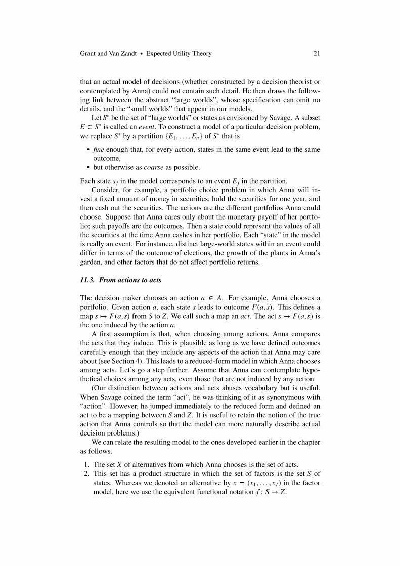
1. The set X of alternatives from which Anna chooses is the set of acts.2. This set has a product structure in which the set of factors is the set S of

states. Whereas we denoted an alternative by x = (x1, . . . , xJ ) in the factormodel, here we use the equivalent functional notation f : S → Z.


f

z1

s1

z2

s2

z3

s3

Figure 2. Visualization of an act.

3. In each state, the set of outcomes is the same: Z. In the factor decomposition,this corresponds to the special case in which Xj = X = Z for each factor.

Although mathematically an act is just an element of a product set, it is ap-pealing to visualize an act (when there are finitely many states) as in Figure 2,because it illustrates the unfolding of uncertainty. At the moment of making achoice, Anna stands in a position at or before the root node. Then one of thethree states is realized—that is, one and only one of the branches from the rootnode occurs, leading to the consumption bundle (or, more generally, the outcome)z = f (s).

12. Sure-thing principle and additivity

Since X has a product structure, we can look for an additive representation ofAnna’s preferences �.

12.1. Joint independence

In this setting, the assumption of joint independence was called the sure-thingprinciple by Savage and has also been called the independence axiom (althoughthe latter term has been used for related axioms in other settings). We pointedout that joint independence was a strong assumption when the factors are con-sumption of different goods or consumption in different time periods: one wouldnever insinuate in those settings that joint independence was a normative axiomas opposed to a mere simplifying assumption. However, in this decision problemunder uncertainty, the sure-thing principle is a plausible normative assumption.

With state-contingent consumption, only one of the states will ever be real-ized. It seems natural to most people, barring any mistakes Anna might make,that deciding how to spend the money Anna might earn if she wins a bet does notdepend on what she might do if she loses the bet. We argue this more fully in thefollowing section.

12.2. Dynamic consistency

The notion of dynamic consistency can help us understand the sure-thing princi-ple and judge whether it is a compelling normative axiom. Because our goal isnot to develop a full theory of dynamic consistency for its own sake and becausesuch a framework is notationally intensive when set out formally, we keep the


discussion informal.In Section 3, we stated that (a) our model of static choice also applied to

choosing a once-and-for-all plan in a temporal setting, but that (b) this chapterwas not about making decisions at different decision epochs or the link betweensuch decisions. Consider, however, such a possibility.

We are developing a normative model. Hence, though it would difficult forher to do so, imagine that Anna can envision all the opportunities in which shewill make decisions, that any uncertainty about available actions and outcomesof actions is reflected in her model of a set of states of the world, and that Annaunderstands how uncertainty is resolved over time as she learns new information.(All this would be modeled formally as a decision tree, which means an extensivegame form in which there are moves by nature but otherwise Anna is the onlyplayer.) A plan specifies the actions Anna would choose at each decision epoch(i.e., a plan is the same as a strategy in an extensive game form). Anna can thenenvision all possible plans and choose among them.

Suppose she then begins executing her preferred plan. At each decision epoch,she could reevaluate the plan—that is, consider all continuation plans on thesubtree (subgame) that follows and choose among them. Dynamic consistencymeans that, as long as she has followed the ex ante preferred plan so far, Annanever wishes to deviate from the plan.

This paints an unrealistic picture of the way people actually make decisions.We do not set up a full model and choose among all possible plans. Even inan easily codified situation such as a chess game to be played during an after-noon, the set of possibilities is so large that it overwhelms our ability to envisionand choose among them. Thus, we always have partially formulated plans, weconstantly extend our partial model further into time, we review our availableoptions, and we revise our decisions.

This is all due to the sheer complexity of devising a complete dynamic plan.However, it is fairly well accepted that dynamic consistency is a reasonable nor-mative axiom—something Anna would satisfy if she were infinitely smart andhad unlimited computational power.

Consider a simple situation in which there are six states, {s1, s2, s3, s4, s5, s6},and in which Anna learns whether the state is in E1 ≡ {s1, s2, s3} or in E2 ≡{s4, s5, s6} before choosing an action. She formulates a plan of what action tochoose depending on whether she observes E1 or E2. Each such plan leads to anact.

For a given act f , we can represent the unfolding of information as in Fig-ure 3. Observe that this is not a full decision tree; it depicts a single act and doesnot show the actions available at each decision epoch. Only nature’s moves fromthe decision tree are shown. Behind the scenes we understand that different de-cisions lead to different acts, which means that Anna’s choices determine whichoutcomes are at the leaves. The partial acts f1 and f2 specify the outcomes forthe states in E1 and E2, respectively. We can write f = ( f1, f2).

If Anna is dynamically consistent, then if she observed E1 she will want tostick to her plan. In other words, when choosing among acts defined on the statesin E1 after observing that event, she will still choose f1 among the available acts.It is a fairly compelling assumption that, when she chooses among continuation


f

f1

E1

z1

s1

z2

s2

z3

s3

f2

E2

z4

s4

z5

s5

z6

s6

Figure 3. An act that results from making decisions after observing {E1, E2}.

plans having observed E1, her preferences do not depend on what she thinks shemight have done had E2 been realized instead.

No theorem states that an infinitely smart person capable of such complexplanning could not then be influenced in her decisions at each decision epoch bythe plans she had made if other contingencies had been realized. “Fairly com-pelling assumption” simply means that these authors (at least) imagine that if wewere so smart then this is how we would make decisions.

This assumption, combined with dynamic consistency, implies that if ( f1, f2) �( f ′1, f2) then also ( f1, f ′2) � ( f ′1, f ′2) for any other partial act f ′2 defined on thestates in E2. More generally, it implies that preferences over acts satisfy the sure-thing principle.

12.3. Expected utility representation with state-dependent utility

Assume now that the sure-thing principle holds (along with other technical as-sumptions, such as those in Theorem 3), so that Anna’s preferences over actshave an additive representation ∑J

j=1 uj(x j), which we may write as

U ( f ) = ∑s∈S

us( f (s)).

Let Π : S → R be any probability measure on S such that Π(s) > 0 for all s ∈ S.For each s ∈ S, define vs : Z → R by vs(z) = us(z)/Π(s). Then

U ( f ) = ∑s∈S

Π(s) vs( f (s)). (11)

Written this way, it it tempting to interpret U as an expected utility representation.Anna’s utility in state s is vs( f (s)) and, given the probability measure Π on states,U ( f ) is the expected value of Anna’s utility. However, since the probability mea-sure was chosen arbitrarily, the probabilities or beliefs used in this representationare indeterminate. Therefore, we cannot claim to have uncovered Anna’s beliefsfrom her preferences.

The problem arises because the utility functions us in the additive represen-tation have no link to each other. Utility is therefore said to be state dependent.


12.4. Expected utility representation with state-independent utility

On the other hand, suppose that the representation satisfies cardinal uniformityacross states and can thus be written as

U ( f ) = ∑s∈S

Δsu( f (s)),

where Δs > 0 for all s and u : Z → R. We then say that the utility is state indepen-dent. We can normalize the weights {Δs | s ∈ S} so that they sum to 1 by settingΠ(s) = Δs/(∑s′∈S Δs′ ); this is equivalent to multiplying the utility representationby 1/(∑s′∈S Δs′ ). Then we have the representation

V ( f ) = ∑s∈S

Π(s) u( f (s)). (12)

If we take another additive representation, we know that it is a positive affinetransformation of V . When we retain the restriction that the weights Π sum to1, the multiplicative and additive constants must end up in the function u. Thus,any additive representation of the preferences can be written in the form of (12)and will always end up with the same weighting function Π. It then becomesmore plausible to refer to these weights as probabilities or beliefs because theyare uniquely identified.

12.5. Is identification of beliefs important?

The answer is both “no” and “yes”, as we now explain.

Identification is a leap of faith. Although the weights Π in representation (12) areuniquely defined, their interpretation as beliefs remains a leap of faith. We cannotfully disentangle—from preferences over acts—whether Anna cares about whathappens in a state because she considers the state likely or because the state affectsher feelings. This is a general point, but we can give a concrete technologicalexample in which preferences have the representation in equation (12) yet theweights Π(s) do not represent beliefs. Let the elements of Z be inputs in a single-output production process that is affected by state-contingent shocks such thatoutput in state s, given inputs z ∈ Z, is Θsu(z) (i.e., the production function in states is z �→ Θsu(z)). An act is a state-contingent input plan f : S → Z. Anna’s beliefsare given by Π, and she is a risk-neutral expected utility maximizer with respectto output. Then her preferences over state-contingent input plans are given by

V ( f ) = ∑s∈S

Π(s) Θs u( f (z)).

The weights Π(s) Θs, written as Π(s) in equation (12), confound probabilities andproductivity shocks. This is an argument that Karni (1985) gives in favor of study-ing state-dependent preferences and utility as opposed to inferring beliefs from anormalization of weights that is not derived from preferences or choice behavior.


Identification of beliefs is not needed for Bayesian decision making. Are weconcerned merely that Anna act as if she were probabilistically sophisticatedand maximized expected utility, so that we can apply the machinery of Bayesianstatistics to Anna’s dynamic decision making? Or rather is our objective to uniquelyidentify her beliefs?

The latter might be useful if we wanted to measure beliefs from empiricallyobserved choices in one decision problem in order to draw conclusions about howAnna would act in another decision problem. Otherwise, the former is typicallyall we need, and state-dependent preferences are sufficient.

We can pick an additive representation of the form (11) with any weights Π.Suppose that Anna faces a dynamic decision problem in which she can revise herchoices at various decision nodes after learning some information (representedby a partition of the set of states). Given dynamic consistency, she will makethe same decisions whether she makes a plan that she must adhere to or insteadrevises her decisions conditional on her information at each decision node. Fur-thermore, in the latter case her preferences over continuation plans will be givenby expected utility maximization with the same state-dependent utilities and withweights (beliefs) that are revised by Bayesian updating. This may allow the an-alyst to solve her problem by backward induction (dynamic programming or re-cursion), thereby decomposing a complicated optimization problem into multiplesimpler problems.

Yet state independence is a powerful restriction. The real power of state-independentutility comes from the structure and restrictions that this imposes on preferences,particularly in equilibrium models with multiple decision makers. We alreadydiscussed this in the context of an intertemporal model with cardinally uniformutility. Let’s revisit this point in the context of decision making under uncertainty.

With state-independent utility, we can separate the relative probabilities of thestates from the preferences over outcomes. For example, when the outcomes aremoney, we can separate beliefs from risk preferences. This is particularly power-ful in a multi-person model because we can then give substance to the assumptionthat all decision makers have the same beliefs. Consider a general equilibriummodel of trade in state-contingent transactions, such as insurance or financialsecurities. Suppose that all traders have state-independent utility with the samebeliefs but heterogeneous utilities over money. If the traders’ utilities are strictlyconcave (they are risk averse) and if the total amount of the good that is avail-able is state independent (no aggregate uncertainty), then in any Pareto efficientallocation each trader’s consumption is state independent (each trader bears norisk).

State independence is without loss of generality (more or less). It can be arguedthat state independence is without loss of generality: if it is violated, one canredefine outcomes to ensure that the description of an outcome includes every-thing Anna cares about—even things that are part of the description of the state.However, when this is done some acts are clearly hypothetical.

Perhaps the two states are “Anna’s son has a heart attack” and “Anna’s sonheart is just fine”. What Anna controls is whether her son has heart surgery.


Clearly her preferences for heart surgery depend on whether or not her son has aheart attack. However, we can define an outcome so that it is specified both bywhether her son has a heart attack and by whether he undergoes the surgery. Inorder to maintain the assumption that the set of acts is the set of all functions fromstates to outcomes, Anna must be able to contemplate and express preferencesamong such hypothetical acts as the one in which her son has a heart attack andgets heart surgery in both states, including the state in which he does not have aheart attack!

Furthermore, when decision under uncertainty is applied to risk and risk shar-ing, the modeler assumes that preferences over money are state independent. Thisis a strong assumption even if preferences were state independent for some ap-propriately re-defined set of outcomes.

13. Lotteries

13.1. From subjective to objective uncertainty

We postpone until Section 14 a discussion of the axioms that capture state in-dependence of preferences and yield a state-independent representation U ( f ) =∑s∈S Π(s) u( f (s)). In the meantime, we consider how state independence com-bined with objective uncertainty allows for a reduced-form model in which choicesamong state-dependent outcomes (acts) is reduced to choices among probabilitymeasures on outcomes (lotteries). We then axiomatize expected utility for sucha model.

One implication of state-independent expected utility is that preferences de-pend only on the probability measures over outcomes that are induced by theacts. That is, think of an act f as a random object whose distribution is the in-duced probability measure p on Z. Assume that S and Z are finite, so that thisdistribution is defined by p(z) = Π{s ∈ S | f (s) = z}. We can then rewriteU ( f ) = ∑s∈S Π(s) u( f (s)) as ∑z∈Z p(z) u(z). In particular, Anna is indifferent be-tween any two acts that have the same induced distribution over outcomes.

Let us now take as our starting point that Anna’s decision problem reducesto choosing among probability measures over outcomes—without a presumptionof having identified an expected utility representation in the full model. We thenstate axioms within this reduced form that lead to an expected utility representa-tion.

For this to be an empirical exercise (i.e., in order to be able to elicit prefer-ences or test the theory), the probability measures over outcomes must be observ-able. This means that the probabilities are generated in an objective way, such asby flipping a coin or spinning a roulette wheel. Therefore, this model is typicallyreferred to as one of objective uncertainty. The other reason to think of this asa model of objective uncertainty is that we will need data on how the decisionmaker would rank all possible distributions over Z. This is plausible only if wecan generate probabilities using randomization devices.

Thus, the set of alternatives in Anna’s choice problem is the set of probabil-ity measures defined over the set Z of outcomes. To avoid the mathematics of


p

z1

p1

z2

p2

z3

p3

Figure 4. A lottery.

measure theory and abstract probability theory, we continue to assume that Z isfinite, letting n be the number of elements. We call each probability measure onZ a lottery.

Let P be the set of lotteries. Each lottery corresponds to a function p : →[0, 1] such that ∑z∈Z p(z) = 1. Each p ∈ P can equivalently be identified with thevector in Rn of probabilities of the n outcomes. The set P is called the simplex inRn; it is a compact convex set with n − 1 dimensions.

We can illustrate a lottery graphically as in Figure 4. The leaves correspondto the possible outcomes and the edges show the probability of each outcome.Figure 4 looks similar to the illustration of an act in Figure 2, but the two figuresshould not be confused. When Anna considers different acts, the states remainfixed in Figure 2 (as do their probabilities); what change are the outcomes. WhenAnna considers different lotteries, the outcomes remain fixed in Figure 4; whatchanges are the probabilities. This reduced-form model of lotteries has a flexibil-ity with respect to possible probability measures over outcomes that would notbe possible in the states model unless the set of states were uncountably infiniteand beliefs were nonatomic.

By an expected utility representation of Anna’s preferences � on P we meanone of the form

U (p) = ∑z∈Z

p(z) u(z),

where u : Z → R. Then U (p) is the expected value of u given the probabilitymeasure p on Z. We call this a Bernoulli representation because Bernoulli (1738)posited such an expected utility as a resolution to the St. Petersburg paradox:that a decision maker would prefer a finite amount of money to a gamble whoseexpected payoff was infinite. Bernoulli took the utility function u : Z → R as aprimitive and expected utility maximization as a hypothesis. His innovation wasto allow for an arbitrary, even bounded, function u : Z → R for lotteries overmoney rather than a linear function, thereby avoiding the straitjacket of expectedvalue maximization—the state of the art in his day.

Expected utility did not receive much further attention until von Neumannand Morgenstern (1944) first axiomatized it (for use with mixed strategies ingame theory). For this reason, the representation is also called a von Neumann–Morgenstern utility function. As we do here, von Neumann and Morgensterntook preferences over lotteries as a primitive and uncovered the expected utilityrepresentation from several axioms on those preferences.


13.2. Linearity of preferences

Recall that P is a convex set and recall from Section 9 that � admits a linearutility representation if if it satisfies the linearity and Archimedean axioms. Weproceed as follows.

1. We observe that a linear utility representation is the same as a Bernoulli rep-resentation.

2. We discuss the interpretation of the linearity and Archimedean axioms.

In this setting, linearity (Axiom L) is called the independence axiom.So suppose we have a linear utility representation

U (p) = ∑z∈Z

uz pz

of Anna’s preferences. We can write the vector {uz | z ∈ Z} of coefficients asa function u : Z → R and use the functional form p : Z → [0, 1] of a lottery p.Then the linear utility representation can be written as

U (p) = ∑z∈Z

p(z) u(z), (13)

that is, as a Bernoulli representation. Like any additive representation, this oneis unique up to a positive affine transformation; such a transformation of U cor-responds to an affine transformation of u. All this is summarized in our nexttheorem.

Theorem 6. If � satisfies the linearity (independence) and Archimedeanaxioms, then � has a Bernoulli representation.

Proof. This is an application of Theorem 5; as such, it is due to Jensen (1967,Thm. 8). Von Neumann and Morgenstern’s representation theorem used a dif-ferent set of axioms that implied but did not contain an explicit independence(linearity) axiom like our Axiom L. The role of the independence axiom, whichwe interpret further in what follows, was uncovered gradually by subsequent au-thors. See Fishburn and Wakker (1995) for a history of this development. �

13.3. Interpretation of the axioms

The convex combinations that appear in the linearity and Archimedean axiomshave a nice interpretation in our lotteries setting. Suppose the uncertainty bywhich outcomes are selected unfolds in two stages. In a first stage, there is arandom draw to determine which lottery is faced in a second stage. With proba-bility α, Anna faces lottery p in the second stage; with probability 1−α she faceslottery r. This is called a compound lottery and is illustrated in Figure 5.

Consider the overall lottery t that Anna faces ex ante, before any uncertaintyunfolds. The probability of outcome z1 (for example) is t1 = αp1 + (1− α)r1. Asa vector, the lottery t is the convex combination αp + (1 − α)r of p and r. Thus,we can interpret convex combinations of lotteries as compound lotteries.


t

p

z1

p1

z2

p2

z3

p3

r

z1

r1

z2

r2

z3

r3

Figure 5. A compound lottery.

t ′

q

z1

q1

z2

q2

z3

q3

r

z1

r1

z2

r2

z3

r3

Figure 6. Another compound lottery.

Consider this compound lottery and the one in Figure 6, recalling the dis-cussion of dynamic consistency and the sure-thing principle from Section 12.Suppose Anna chooses t over t ′ and then, after learning that she faces lottery pin the second stage, is allowed to change her mind and choose lottery q instead.Dynamic consistency implies that she would not want to do so. Furthermore,analogous to our normative justification of the sure-thing principle, it is also nat-ural that her choice between p and q at this stage would depend neither on whichlottery she would otherwise have faced along the right branch of the first stagenor on the probability with which the left branch was chosen. Together, these twoobservations imply that she would choose lottery t over t ′ if and only if she wouldchoose lottery p over q. Mathematically, in terms of the preference ordering �,this is Axiom L. It is called the independence axiom or substitution axiom in thissetting because the choices between t and t ′ are then independent of which lotterywe substitute for r in Figure 6.

Thus, the justification for the independence (linearity) axiom in this lotteriesmodel is the same as for the sure-thing principle (joint independence axiom) inthe states model, but the two axioms are mathematically distinct because the twomodels define the objects of choice differently (lotteries vs. acts).

The Archimedean axiom has the following meaning. Suppose that Annaprefers lottery p over lottery q. Now consider the compound lottery t in Fig-ure 6. Lottery r might be truly horrible. However, if the Archimedean axiom issatisfied then, as long as the right branch of t occurs with sufficiently low prob-ability, Anna still prefers lottery t over lottery q. This is illustrated by the risk of


death that we all willingly choose throughout our lives. Death is certainly some-thing “truly horrible”; however, every time we cross the street we choose a lotterywith small probability of death over the lottery we would face by remaining onthe other side of the street.

13.4. Calibration of utilities

The objective probabilities are used in this representation to calibrate the decisionmaker’s strength of preference over the outcomes. To illustrate how this is done,suppose Anna is considering various alternatives that lead to varying objectivelymeasurable probabilities of the following outcomes:

e — Anna stays in her current employment;m — Anna gets an MBA but then does not find a better job;M — Anna gets an MBA and then finds a much better job.

We let Z = {e, m, M} be the set of outcomes and, since this is a reduced form,we view her choice among her actions as boiling down to the choice among theprobabilities over Z that the actions induce. Furthermore, we suppose that she cancontemplate choices among all probability measures on Z, and not merely thoseinduced by one of her actions. We assume M � e � m, where (for example)M � e means that she prefers getting M for sure to getting e for sure.

Anna’s preference for e relative to m and M can be quantified as follows. Wefirst set u(M) = 1 and u(m) = 0. We then let u(e) be the unique probability forwhich she is indifferent between getting e for sure and the lottery that yields Mwith probability u(e) and m with probability 1 − u(e)—that is, for which e ∼u(e)M + (1−u(e))m. The closer e is to M than to m in her strength of preference,the greater this probability u(e) would have to be and, in our representation, thegreater is the utility u(e) of e.

The Archimedean axiom implies that such a probability u(e) exists. The in-dependence axiom then implies that the utility function u : Z → R thus definedyields a Bernoulli representation of Anna’s preferences. The actual proof of therepresentation theorem is an extension of this constructive proof to more generalZ.

14. Subjective expected utility without objective probabilities

14.1. Overview

Let us return to the states and acts setting of Sections 11 and the state-dependentexpected utility representation from Section 12. Recall the challenge—posed butnot resolved—of finding a state-independent representation, so that the probabil-ities would be uniquely identified and could be interpreted as beliefs revealed bythe preferences over acts. This is called subjective expected utility (SEU).

One of the first derivations of subjective expected utility (involving the jointderivation of subjective probabilities to represent beliefs about the likelihood ofevents as well as the utility index over outcomes) appeared in a 1926 paper by


Frank Ramsey, the English mathematician and philosopher. This article was pub-lished posthumously in Ramsey (1931) about the same time that an independentbut related derivation appeared in Italian by the statistician de Finetti (1931).The definitive axiomatization in a purely subjective uncertainty setting appearedin Leonard Savage’s 1954 book, The Foundation of Statistics.

In Section 12, we showed that the sure-thing principle implied additivity ofthe utility. We went on to say that SEU requires that the additive utility be cardi-nally uniform across states, but we stopped before showing how to obtain such aconclusion. Recall further back to Section 10, where we tackled cardinal unifor-mity in the abstract factors setting. Axiomatizing cardinal uniformity was tricky,but we outlined three solutions. Each of those solutions corresponds to an ap-proach taken in the literature on subjective expected utility.

1. Savage (1954) used an infinite and nonatomic state space as in Section 10.3.We develop this further in Section 14.2.

2. Wakker (1989) assumed a connected (hence infinite) set of outcomes andassumed cardinal coordinate independence, as we did in Section 10.4. Car-dinal coordinate independence involves specific statements about how thedecision maker treats trade-offs across different states and assumes that suchtrade-offs are state independent.

3. Anscombe and Aumann (1963) mixed subjective and objective uncertaintyto obtain a linear representation, as in Section 10.5. We develop this in Sec-tion 15.

14.2. Savage

We give a heuristic presentation of the representation in Savage (1954). (In whatfollows, Pn refers to Savage’s numbering of his axioms.) Savage began by as-suming that preferences are transitive and complete (P1: weak order) and satisfyjoint independence (P2: sure-thing principle); this yields an additive or state-dependent representation. The substantive axioms that capture state indepen-dence are ordinal uniformity (P3: ordinal state independence) and joint rankingof factors (P4: qualitative probability).

As a normative axiom, P3 is really a statement about the ability of the modelerto define the set of outcomes so that they encompass everything that Anna caresabout. Then, given any realization of the state, Anna’s preferences over outcomesshould be the same.

Because Savage works with an infinite state space in which any particularstate is negligible, his version of P3 is a little different from ours and he needs anadditional related assumption. These are minor technical differences.

1. Savage’s P3 states that Anna’s preferences are the same conditional on anynonnegligible event, rather than on any state. With finitely many states, thetwo axioms are equivalent.

2. Savage adds an axiom (P7) that the preferences respect statewise dominance:given Anna’s state-independent ordering �∗ on Z, if f and g are such thatf (s) �∗ g(s) for all s ∈ S then f � g. With finitely-many states, this condi-tion is implied by the sure-thing principle and ordinal state independence.


Let consider in more detail Savage’s P4, which is our joint ranking of fac-tors. We begin by restating this axiom using the terminology and notation of thepreferences-over-acts setting.

Axiom 5 (Qualitative probability). Suppose that preferences satisfy ordinal stateindependence and let �∗ be the common-across-states ordering on Z. Let A, B ⊂S be two events. Suppose that z1 �∗ z2 and z3 �∗ z4. Let, for example, (IAz1, IAc z2)be the act that equals z1 on event A and z2 on its complement. Then

(IAz1, IAc z2) � (IBz1, IBc z2) ⇐⇒ (IAz3, IAc z4) � (IBz3, IBc z4).

This axiom takes state independence one step further: it captures the ideathat the decision maker cares about the states only because they determine thelikelihood of the various outcomes determined by acts. If preferences are stateindependent, then the only reason Anna would prefer (IAz1, IAc z2) to (IBz1, IBc z2)is because she considers event A to be more likely than event B. In such case, shemust also prefer (IAz3, IAc z4) to (IBz3, IBc z4).

As explained in Section 10.3, ordinal state independence and qualitative prob-ability impose enough restrictions to yield state-independent utility only if thechoice set is rich enough—with one approach being to have a nonatomic set offactors or states. This is the substance of Savage’s axiom P6 (continuity). Thericher state space allows one to calibrate beliefs separately from payoffs over theoutcomes.

15. Subjective expected utility with objective probabilities

15.1. Horse-race/roulette-wheel lotteries

Anscombe and Aumann (1963) avoided resorting to an infinite state space oraxioms beyond joint independence and ordinal uniformity by combining (a) alotteries framework with objective uncertainty and (b) a states framework withsubjective uncertainty.

In their model, an act assigns to each state a lottery with objective probabili-ties. These two-stage acts are also called horse-race/roulette-wheel lotteries, butwe continue to refer to them merely as acts and to the second-stage objective un-certainty as lotteries. Fix a finite set S of states and a finite set Z of outcomes. Welet P be the set of lotteries on Z. An act is a function f : S → P. Let H be the setof acts.

15.2. Linearity: sure-thing principle and independence axiom

First notice that H, which is the product set PS, is also a convex set and thatthe convex combination of two acts can be interpreted as imposing compoundlotteries in the second (objective) stage of the unfolding of uncertainty. In otherwords, for any pair of acts f , g in H and any α in [0, 1], α f + (1−α)g correspondsto the act h in H for which h(s) = α f (s)+ (1−α)g(s), where α f (s)+ (1−α)g(s)is the convex combination of lotteries f (s) and g(s).


In Section 9, we showed that � has a linear utility representation if � satisfiesthe linearity and Archimedean axioms. Let us consider the interpretation of sucha utility representation and the interpretation of these axioms.

The dimensions of H are S×Z and a linear utility function on H can be writtenas

∑s∈S

∑z∈Z

usz psz = ∑s∈S

∑z∈Z

usz × f (s)(z). (14)

On the left side, we have represented the element of H as a vector p ∈ RS×Z; theprobability of outcome z in state s is psz. On the right side, we have representedthe element of H as an act f : S → P; the probability of outcome z in state s isf (s)(z). (That is, f (s) is the probability measure or lottery in state s and f (s)(z) isthe probability assigned to z by that measure.) We used a “×”’ on the right-handside for simple multiplication to make clear that f (s)(z) is a single scalar term.The order of summation in equation (14) is irrelevant.

For any probability measure Π on S we can also write the linear utility functionin the form

∑s∈S

Π(s) ∑z∈Z

f (s)(z) × us(z). (15)

We derived equation (15) from (14) by:

• dividing each coefficient usz by Π(s) and writing the result as us(z); then• reversing the order of multiplication so that ∑z∈Z f (s)(z)×us(z) is recognized

as the expected utility in state s—given that f (s) is the probability measureon Z and us : Z → R is the utility function on Z in state s.

Thus, (15) can be interpreted as the subjective expected value (over states S withsubjective probability Π) of the objective expected utility (over outcomes Z givenobjective probabilities f (s) in state s). We call equation (15) a state-dependentAnscombe–Aumann representation. We thus have, as a corollary to Theorem 5and this discussion, the following representation theorem.

Theorem 7. Assume that � satisfies the linearity and Archimedean axioms.Then � has a state-dependent Anscombe–Aumann representation.

The linearity axiom on � thus encompasses two independence conditions:

1. the sure-thing principle as applied to subjective uncertainty across differentstates (that is, linearity implies joint independence over factors, as shown inSection 9.4);

2. the independence axiom as applied to objective uncertainty within each state(that is, linearity of � implies linearity of the within-state preferences).

The normative arguments that justify these two axioms or principles, which wehave already discussed extensively, also justify the linearity axiom in this Anscombe–Aumann framework.


15.3. State independence

The probability measure Π is still not uniquely identified because we have state-dependent utility. However, recall from Section 10.5 that the additional assump-tion of ordinal state independence is enough to obtain state-independent linearutility and thus to pin down the subjective beliefs. The overall representationbecomes

U ( f ) = ∑s∈S

Π(s) ∑z∈Z

f (s)(z) × u(z). (16)

We call equation (16) an Anscombe–Aumann representation.We summarize this as follows.

Theorem 8. Assume that � satisfies the linearity, Archimedean, and ordinalstate independence axioms. Then � has an Anscombe–Aumann representation.

Proof. This follows from Theorem 5 and the preceding discussion. It is alsoessentially Anscombe and Aumann (1963, Thm. 1) though their axiomatizationis a bit different. �

15.4. Calibration of beliefs

The simplicity of Theorem 8 and the fact that it is a mere application of linearutility masks the way in which beliefs and utilities are disentangled. We illustratehow such calibration happens using ideas that lurk in the proof of the theorem.

For example, consider a less reduced-form version of the story in Section 13.4.Anna chooses between two actions:

leave — leaving her current employment to undertake an MBA;stay — staying put.

The relevant outcomes are the three enumerated in Section 13.4: (e) no MBA andstaying in her current employment; (m) bearing the cost of an MBA without thenfinding a better job; and (M) bearing the cost of an MBA and then finding a betterjob.

The last element in the decision problem is the event E , the set of states inwhich Anna obtains the better job if she gets an MBA. We take this to be a stateor elementary event in the small-worlds model; hence the set of states is {s1, s2},where s1 corresponds to event E and s2 corresponds to event Ec. Therefore thetwo acts associated with the actions leave and stay are

leave(s1)=M, leave(s2)=m;

stay(s1)=e, stay(s2)=e.

Whether we have leave � stay or stay � leave seems to depend on two sep-arate considerations. How good Anna feels the chances of obtaining a better jobwould have to be in order to make it worthwhile to leave her current employment;and how good in her opinion the chances of obtaining a better job actually are.What Anna does when she answers the former question is quantify her personal


preference for e relative to m and M. What Anna does when she answers the latterquestion is quantify her personal judgment concerning the relative strengths ofthe factors that favor and oppose certain events.

In order to calibrate these two considerations, we must assume that she canmeaningfully compare any horse-race/lottery acts, nor merely the acts leave andstay available to her in this problem. Thus, she must be able to express prefer-ences over hypothetical acts such as the act

g(s1) = m, g(s2) = M,

(in the state s2 where she would not find a good job if she got an MBA, she getsan MBA and finds a good job!) and the act that yields, in both states, a lotterywith equal probability of the three outcomes.

We can first quantify the strength of Anna’s personal preference for e relativeto m and M by considering the constant acts (lotteries that are not state depen-dent). That is, we abstract from the subjective uncertainty about the states andconsider her preferences over objectively generated lotteries. This is the repre-sentation and calibration we covered in Section 13. We thereby let u(m) = 0 andu(M) = 1 and define u(e) to be such that Anna is indifferent between e and thelottery u(e)M + (1 − u(e))m.

To quantify Anna’s judgment concerning the likelihood of state s1, we letΠ(s1) be the unique probability for which Anna is indifferent between the act leaveand the act that leads, in every state, to the lottery with probability Π(s1) on M andprobability 1− Π(s1) on m. The idea is that, given state-independent preferences,the state is simply a randomization device from Anna’s point of view: if Anna isindifferent between these two acts, it is because the objective probability Π(s1) isthe same as Anna’s subjective likelihood of state s1.

16. Conclusion

Throughout this chapter we have emphasized the link between independence ax-ioms in standard consumer theory, in expected utility theory for decision underobjective uncertainty, and in expected utility theory for decision under subjec-tive uncertainty. We contend that the independence axioms have considerablenormative appeal in decision under uncertainty.

However, experimental and empirical evidence shows that behavior deviatessystematically from these theories, implying that (not surprisingly) such norma-tive theories make for only approximate descriptive models. Furthermore, manyauthors have disagreed with our claim that the independence axioms are norma-tively compelling.

There is now a vast literature that has developed generalizations, extensions,and alternatives to expected utility. We will not provide a guide to this literature;doing so would be beyond the scope of our chapter whereas later chapters in thishandbook treat it extensively. However, as a transition to those chapters and as afurther illustration of the content of the independence axioms, we outline someof the experimental violations.

One of the earliest and best known tests of expected utility is the common


Lottery Simple form Compound form

I Prob. Prize

.66 $50,000

.33 $53,000

.01 $0 $50,000

.66 .34

$53,000

33/34

$0

1/34

II Prob. Prize

1 $50,000

$50,000

.66

$50,000

.34

III Prob. Prize

.67 $0

.33 $53,000

$0

.66 .34

$53,000

33/34

$0

1/34

IV Prob. Prize

.66 $0

.34 $50,000

$0

.66

$50,000

.34

Figure 7. Common consequence paradox (Allais paradox): The simple lotteries on the left are thereduced lotteries of the compound lotteries on the right. Preferences II � I and III � IV violate theindependence axiom but are common for subjects in decision experiments.


Lottery Simple form Compound form

I Prob. Prize

.2 $0

.8 $4,000

$0

.2

$4,000

.8

II Prob. Prize

1 $3,000

$3,000

1

III Prob. Prize

.8 $0

.2 $4,000

$0

.75 .25

$0

.2

$4,000

.8

IV Prob. Prize

.75 $0

.25 $3,000

$0

.75 .25

$3,000

1

Figure 8. Common ratio paradox: The simple lotteries on the left are the reduced lotteries of thecompound lotteries on the right. Preferences II � I and III � IV violate the independence axiom butare common for subjects in decision experiments.

consequence paradox, first proposed by Maurice Allais (1953). It is illustrated inFigure 7. Allais conjectured (and found) that most people would prefer lottery IIto lottery I but would prefer lottery III to lottery IV (when presented as the simplelotteries on the left). By writing the simple lotteries as the compound lotteries onthe right, we can see that such choices violate the independence axiom (AxiomL).

A closely related and frequently observed systematic violation of expectedutility theory is the common ratio paradox (see Kahneman and Tversky 1979).This is illustrated in Figure 8. Again, the choices of II over I and III over IV arecommon but violate the independence axiom.

There has been debate about whether these violations are due to boundedrationality or whether the normative model needs adjustment, but there certainlyroom for better descriptive models than the classic theory reviewed in this chapter(even if, for many applications, the classic theory has proved to be a suitablyaccurate approximation).

Systematic violations of expected utility theory—observed in choice prob-


lems such as these paradoxes—suggests the following: when altering a lottery byreducing the probability of receiving a given outcome, the portion of the proba-bility we must place on a better outcome (with the remaining portion on a worseoutcome) in order to keep the individual indifferent is not independent of thelottery with which we began. Yet the independence axiom implies that it is inde-pendent. Indeed, for any three outcomes H, M, L, with H � M � L, the trade-offfor an expected utility maximizer is simply the constant slope of the indifferencecurves in the simplex of lotteries:

u(M) − u(L)u(H) − u(M)

.

When assessing the accumulated experimental evidence, Machina (1982) pro-posed that one could account for these observed systematic violations of expectedutility by assuming that this trade-off is increasing the “higher up” (in preferenceterms) in the simplex is the lottery with which one starts. Geometrically, this cor-responds to a “fanning out” of the indifference curves in the simplex. Many otherpatterns have been observed that depend on the size and sign of the payoffs.

In response, several versions of so-called non- or generalized expected utilityhave axiomatized and analyzed nonlinear representations of preferences over lot-teries. These include, among others, rank dependent expected utility of Quiggin(1982) and Yaari (1987), cumulative prospect theory of Tversky and Kahneman(1992) and Wakker and Tversky (1993), betweenness of Dekel (1986) and Chew(1989), and additive bilinear (regret) theories of Loomes and Sugden (1982) andFishburn (1984).

Another famous experiment, whose results are inconsistent with subjectiveexpected utility theory, is the Ellsberg paradox. Daniel Ellsberg (1961) proposeda number of thought experiments to suggest that, in situations with ambiguityabout the nature of the underlying stochastic process, preferences over subjec-tively uncertain acts would not allow for beliefs over the likelihood of events tobe represented by a well-defined probability distribution.

One such choice problem involves an urn from which a ball will be drawn.Anna knows there are 90 balls in total, of which 30 are red. However, the onlyinformation she has about the remaining 60 balls is that some are black and someare white—she is not told the actual proportions. Consider two choice problems.

1. A choice between ( f ) an act that pays $100 dollars if the ball drawn is redand nothing if it black or white, and (g) an act that pays $100 dollars if theball drawn is black and nothing if it is red or white.

2. A choice between ( f ′) an act that pays $100 dollars if the ball drawn is redor white and nothing if it is black, and (g′) an act that pays $100 dollars ifthe ball drawn is black or white and nothing if it is red.

Ellsberg conjectured that many individuals would be averse to ambiguity inthe sense that they would prefer to bet on “known” rather than “unknown” odds.In this example, they would strictly prefer the bet on red to the bet on black in thefirst problem ( f � g)—indicating a subjective belief that black is less likely thanred—but then prefer the bet on black or white to the bet on red or white in thesecond problem (g′ � f ′)—indicating a subjective belief that black is more likely


than red. As indicated, such a preference pattern is inconsistent with beliefs beingrepresented by a well-defined probability measure.

In response, models have been developed in which beliefs are represented bymultiple measures and/or nonadditive capacities (which is a generalization of aprobability measure). Examples are Gilboa and Schmeidler (1989) and Schmei-dler (1989).

We have mentioned only a small sample of critiques of classic expected utilitytheory reviewed and of the extensions to that theory. This theme is developedfurther in other chapters of this handbook.

References

Allais, Maurice (1953). La psychologie de l’homme rationnel devant le risque: critiquedes postulats et axiomes de l’école Américaine. Econometrica, 21, 503–546.

Anscombe, F.J. and R.J. Aumann (1963). A Definition of Subjective Probability. Annalsof Mathematical Statistics, 34, 199–205.

Arrow, Kenneth J. (1959). Rational Choice Functions and Orderings. Economica, 26,121–127.

Bernoulli, Daniel (1738). Specimen Theoriae Novae de Mensura Sortis. CommentariiAcademiae Scientiarum Imperialis Petropolitanae, 5, 175–192.

Birkhoff, Garrett (1948). Lattice Theory. New York: American Mathematical Society.Cantor, Georg (1895). Beiträage zur Begründung der trans nieten Mengenlehre I. Math-

ematische Annalen, 46, 481–512.Chew, Soo Hong (1989). Axiomatic Utility Theories with the Betweenness Property.

Annals of Operations Research, 19, 273–298.de Finetti, Bruno (1931). Sul Significato Soggettivo della Probabilità. Fundamenta Math-

ematicae, 17, 298–329.Debreu, Gerard (1954). Representation of a Preference Ordering by a Numerical Function.

In R. M. Thrall, C. H. Coombs, and R. L. Davis (Eds.), Decision Processes, pp. 159–165. New York: Wiley.

Debreu, Gerard (1960). Topological Methods in Cardinal Utility Theory. In K. J. Arrow,S. Karlin, and P. Suppes (Eds.), Mathematical Methods in the Social Sciences, 1959,pp. 16–26. Stanford University Press.

Debreu, Gerard (1964). Continuity Properties of Paretian Utility. International EconomicReview, 5, 285–293.

Dekel, Eddie (1986). An Axiomatic Characterization of Preferences under Uncertainty:Weakening the Independence Axiom. Journal of Economic Theory, 40, 304–318.

Ellsberg, Daniel (1961). Risk, Ambiguity, and the Savage Axioms. Quarterly Journal ofEconomics, 75, 643–669.

Fishburn, Peter (1970). Utility Theory for Decision Making. New York: John Wiley &Sons.

Fishburn, Peter (1984). Dominance in SSB Utility Theory. Journal of Economic Theory,34, 130–148.

Fishburn, Peter and Peter Wakker (1995). The Invention of the Independence Conditionfor Preferences. Management Science, 41, 1130–1144.

Gilboa, Itzhak and David Schmeidler (1989). Maxmin Expected Utility with a Non-Unique Prior. Journal of Mathematical Economics, 18, 141–153.

Hammond, Peter J. (1988). Consequentialist Foundations for Expected Utility. Theoryand Decision, 25, 25–78.


Herstein, I.N. and John Milnor (1953). An Axiomatic Approach to Measurable Utility.Econometrica, 21, 291–297.

Jensen, Niels-Erik (1967). An Introduction to Bernoullian Utility Theory, I, II. SwedishJournal of Economics, 69, 163–183, 229–247.

Kahneman, Daniel and Amos Tversky (1979). Prospect Theory: An Analysis of Decisionunder Risk. Econometrica, 47, 263–291.

Karni, Edi (1985). Decision Making under Uncertainty: The Case of State-DependentPreferences. Cambridge, MA: Harvard University Press.

Krantz, David H., R. Duncan Luce, Patrick Suppes, and Amos Tversky (1971). Founda-tions of Measurement, volume I. Additive and Polynomial Representations. NewYork: Academic Press.

Loomes, Graham and Robert Sugden (1982). Regret Theory: An Alternative Theory ofRational Choice under Uncertainty. Economic Journal, 92, 805–824.

Machina, Mark J. (1982). ‘Expected Utility’ Analysis without the Independence Axiom.Econometrica, 50, 277–323.

Quiggin, John (1982). A Theory of Anticipated Utility. Journal of Economic Behaviorand Organization, 3, 323–343.

Ramsey, Frank P. (1931). Truth and Probability. In Foundations of Mathematics and otherLogical Essays. London: K. Paul, Trench, Trubner, and Co.

Samuelson, Paul A. (1938). A Note on the Pure Theory of Consumer’s Behaviour. Eco-nomica, 5, 61–71.

Savage, Leonard J. (1954). The Foundations of Statistics. New York: Wiley.Schmeidler, David (1989). Subjective Probability and Expected Utility without Additivity.

Econometrica, 57, 571–587.Strotz, Robert H. (1959). The Utility Tree—A Correction and Further Appraisal. Econo-

metrica, 27, 482–488.Tversky, Amos and Daniel Kahneman (1992). Advances in Prospect Theory: Cumulative

Representation of Uncertainty. Journal of Risk and Uncertainty, 5, 297–323.von Neumann, John and Oskar Morgenstern (1944). Theory of Games and Economic

Behavior. Princeton, NJ: Princeton University Press.Wakker, Peter (1988). The Algebraic versus the Topological Approach to Additive Rep-

resentations. Journal of Mathematical Psychology, 32, 421–435.Wakker, Peter (1989). Additive Representations of Preferences: A New Foundation of

Decision Analysis. Dordrecht, The Netherlands: Kluwer Academic Publishers.Wakker, Peter and Amos Tversky (1993). An Axiomatization of Cumulative Prospect

Theory. Journal of Risk and Uncertainty, 7, 147–176.Wakker, Peter and Horst Zank (1999). State Dependent Expected Utility for Savage’s

State Space. Mathematics of Operations Research, 24, 8–34.Yaari, Menahem E. (1987). The Dual Theory of Choice under Risk. Econometrica, 55,

95–15.

expected utility theory - rice universityecon501/lectures/decision_eu.pdf · expected utility...

Documents