exercise topic: getting started with hec-hms part 1: create and calibrate a hec-hms runoff model 1....
TRANSCRIPT

1
George Mason University Department of Civil, Environmental and Infrastructure Engineering
Dr. Celso Ferreira
Prepared by Lora Baumgartner December 2015 Revised by Brian Ross July 2016
Exercise Topic: Getting started with HEC-HMS
____________________________________________________________________________________________________________
Objective: Calculate the design hydrograph for a bridge construction project based on the data and instructions given below.
a) Set-up your HMS model
b) Calibrate your model parameters based on the measured data and the Muskingum Method
c) Calculate your design hydrograph
Challenges:
a) Evaluate the impact of land use changes upstream
b) Evaluate the impact of subwatershed changes
c) Explore using different methods for transform, losses and routing.
**Refer to the ArcGIS Resource Center for definitions and context of the steps and tools in this tutorial, currently found in the Help Menu of HEC-HMS.
Tutorial DEM obtained from GMU Campus Lidar file (provided)
Versions used for this tutorial: HEC-HMS 4.0

2
Part 1: Create and Calibrate a HEC-HMS Runoff Model
1. Create a New Project
2. Open the HEC-HMS program and create a new project by clicking on the worksheet icon at the top left of the page.
3. Enter the project name, project description (as needed), the preferred file location, and the preferred unit system.
4. Click “Create”.

3
2. Supporting Data
The basin is composed of four sub-basins, labeled with letters A-D.
The basin contains two reaches, labeled with Roman numerals I – II.
The measured rainfall data for the basin is given to the far right.
The land use and soil type of each
sub-basin is listed to the right.
The attributes of each river reach are listed to the right.

4
The reference table for land use
curve numbers and percent impervious values is shown to the right.

5
The measured discharge data for the
basin is given to the far right.

6
3. Create a Basin
1. Select the “Basin Model Manager” from the Components drop-down menu.
2. Click “New” in the Basin Model Manager window.
3. Enter the new basin name and description (as needed).
4. Click “Create”.
5. Note that a new Basin has been added to the project and close out the window.

7
4. Create Subbasins
1. In the left sidebar Components window, click the plus sign to the left of the “Basin Models” folder and select the newly created basin. The Basin Model diagram window will open to the right.
2. Select the “Subbasin Creation Tool” icon in the top toolbar.
3. Click on the Basin Model window to initiate creation of a subbasin. When the “Create a New Subbasin Element” pops up, fill in the subbasin name and description (as needed).
4. Click “Create”. The new subbasin will be shown on the diagram. Drag the icon to move the subbasin to the preferred location.
5. Repeat steps 10 through 12 to create the remaining three subbasins.
6. In the left sidebar Components, click the plus sign to the left of the Basin folder to show the subbasins.

8
5. Create River Reaches
1. Select the “Reach Creation Tool” icon in the top toolbar.
2. To start the first river reach, click on the Basin model screen in the suggested location (shown at right).
3. To complete the first river reach, click on the Basin model screen in the suggested location (shown at right).
4. Fill in the reach name and description (as needed).
5. Click “Create”.
6. Repeat steps 15 through 19 to create the second river reach. Suggested configuration shown at right.
9
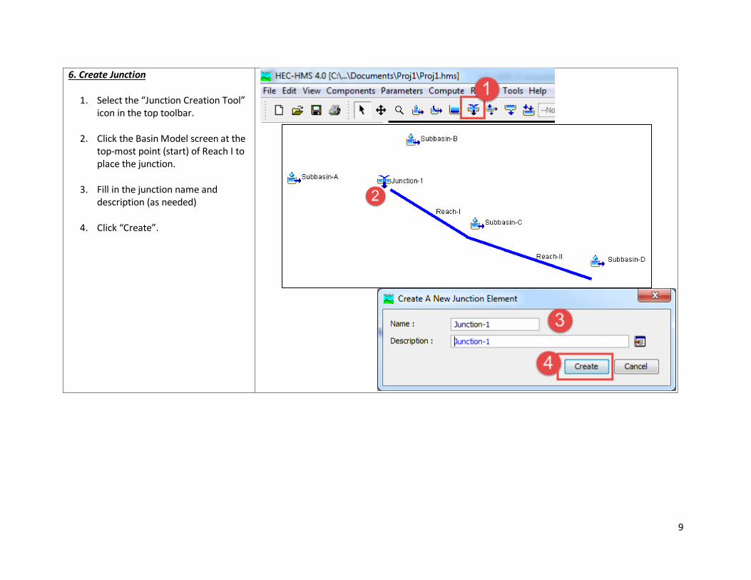
6. Create Junction
1. Select the “Junction Creation Tool” icon in the top toolbar.
2. Click the Basin Model screen at the top-most point (start) of Reach I to place the junction.
3. Fill in the junction name and description (as needed)
4. Click “Create”.

10
7. Create Sink
1. Select the “Sink Creation Tool” icon in the top toolbar.
2. Click the Basin Model screen at the bottom-most point (end) of Reach II to place the sink.
3. Fill in the sink name and
description (as needed).
4. Click “Create”.

11
8. Create Time-Series Data Tables
1. Select the “Time-Series Model Manager” from the Components drop-down menu.
2. Select “Precipitation Gages” from the Data Type drop-down menu.
3. Click “New” in the Time-Series Model Manager window.
4. Enter the new Precipitation Gage name and description (as needed).
5. Click “Create”.
6. Repeat steps 3 through 5 after selecting “Discharge Gages” from the Data Type drop-down menu.
7. Note that a new Discharge Gage has been added to the project and close the window.

12
9. Configure Time-Series Data Tables
1. In the left sidebar Components window, select the plus signs next to the Precipitation Gage menus. Select the Gage.
2. In the Time-Series Gage window below, select “1 Hour” from the Time Interval drop-down menu.
3. In the Components window, select the dated Gage item.
4. In the Time-Series Gage window below, select the tab labeled “Table”.
5. Manually enter the measured rainfall data given in Step 2.
6. Select the tab labeled “Time Window”.
7. Change the End Date to match the Start Date and change the End Time to reflect the length of the measured rainfall.
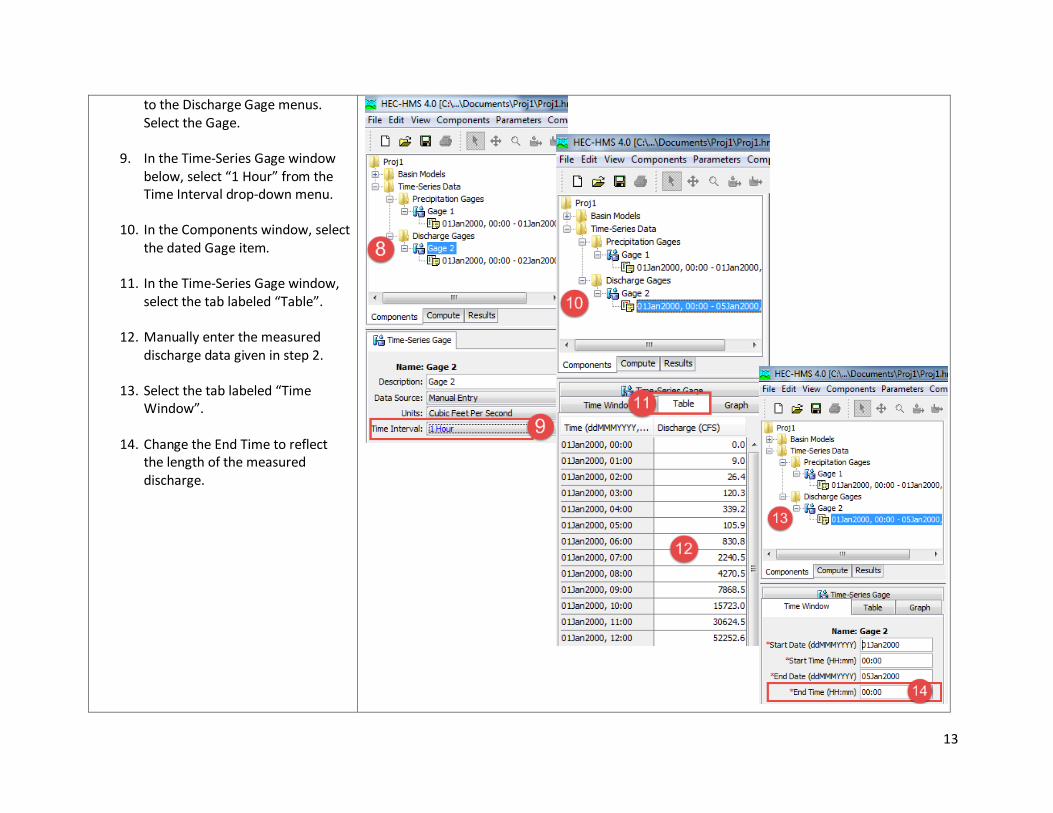
8. In the left sidebar Components window, select the plus signs next
13
to the Discharge Gage menus. Select the Gage.
9. In the Time-Series Gage window below, select “1 Hour” from the Time Interval drop-down menu.
10. In the Components window, select the dated Gage item.
11. In the Time-Series Gage window, select the tab labeled “Table”.
12. Manually enter the measured discharge data given in step 2.
13. Select the tab labeled “Time Window”.
14. Change the End Time to reflect the length of the measured discharge.

14
10. Create a Meteorologic Model
1. Select the “Meteorologic Model Manager” from the Components drop-down menu.
2. Click “New” in the Meteorologic Model Manager window.
3. Enter the new meteorologic model name and description (as needed).
4. Click “Create”.
5. Note that a new meteorologic model has been added to the project and close out the window.

15
11. Configure Meteorologic Model
1. In the left sidebar Components window, select the plus sign next to the Meteorologic Models menu. Select the Met Model.
2. In the Components menu below, select the tab labeled “Meteorology”.
3. Select “Set To Default” from the Replace Missing drop-down menu.
4. Select the tab labeled “Basins”.
5. Select “Yes” from the Include Basins drop-down menu.
6. In the left sidebar Components window, select the “Specified Hyetograph” Met Model item.
7. Under the Subbasins tab, specify the precipitation gage under each subbasin drop-down menu.

16
12. Configure Basin Components This exercise uses the Muskingum method to calculate runoff. Canopy, surface, and baseflow methods are neglected.
1. In the left sidebar Components window, select the plus sign next to the Basin Models menu. Select Subbasin A.
2. Select the tab labeled “Subbasin”.
3. Specify the downstream component as “Junction I”.
4. Enter the surface area of the subbasin as given in Step 2.
5. Select “SCS Curve Number” from the Loss Method drop-down menu.
6. Select “SCS Unit Hydrograph” from the Transform Method drop-down menu.
7. Select the tab labeled “Loss”.
8. Enter the Curve number and Percent Impervious as determined from the land use table given in Step 2 (interpolate as needed).
9. Select the tab labeled

17
“Transform”.
10. Enter the Lag Time as given in Step 2.
11. Repeat Steps 1 through 10 for Subbasins B, C, and D.
Choose Junction I to be downstream of Subbasin B. Choose Reach II to be downstream of Subbasin C. Choose Sink I to be downstream of Subbasin D.
12. Select Junction I. 13. Specify the downstream
component as “Reach I”.
14. Select Reach I.

18
15. Select the tab labeled “Reach”.
16. Specify the downstream
component as “Reach II”.
17. Select “Muskingum” from the Routing Method drop-down menu.
18. Select the tab labeled “Routing”.
19. Enter the values for [Muskingum] K and X as given in Step 2.
20. Repeat steps 14 through 19 for Reach II. (Specify Sink I as downstream.)
21. Select Sink I. 22. Select the tab labeled “Options”. 23. Specify the discharge gage in the
Observed Flow drop-down menu.

19
At this point, the geographical, meteorological, and measured data components of the model have been set.

20
13. Create Control Specifications Manager
1. Select the “Control Specifications Manager” from the Components drop-down menu.
2. Click “New” in the Control Specifications Manager window.
3. Enter the new Control Specifications name and description (as needed).
4. Click “Create”.
5. Note that a new Control Specification has been added to the project and close out the window.

21
14. Configure Control Specification Manager
1. In the left sidebar Components menu, select the Specification Control.
2. Set the timeframe to approximately equal, but not exceed, the start and end times of the measured discharge data given in Step 2.
3. Select “5 Minutes” from the Time Interval drop-down menu.

22
15. Prepare Simulation Run
1. Select the “Simulation Run Manager” from the Compute drop-down menu.
2. Click “New” in the Simulation Run Manager window.
3. Enter the Run name.
4. Click “Next”.
5. Select the preferred Basin.
6. Click “Next”.

23
7. Select the preferred Meteorologic
Model.
8. Click “Next”.
9. Select the preferred Control Specification.
10. Click “Finish”.
11. Note that a new Simulation Run has been created and close the window.

24
16. Run Simulation
1. Select the new Run from the Current Compute Selection drop-down menu.
2. Click the “Compute Current Run” icon.
3. If the computation is successful (e.g. all components are present and configured properly), the progress bar will read 100%. Click Close.
Note that the program has provided several status updates in the Dialogue Box. While the computations were successfully completed, several possible optimizations are recommended.

25
17. View Results
1. In the left sidebar, select the tab labeled “Results”.
2. Click the plus signs to the left of the Simulation Runs menus and select “Global Summary” for the run completed in Step 16.
3. View the summary table of results for the watershed.
4. Select Sink I.
5. Select “Graph” to view the discharge for the watershed and compare the curve of the computation to the curve of the measured discharge data.
Note that the curve of the “Sink I Result: Outflow” peaks slightly earlier and at a greater value than the measured outflow data. Calibration of the Muskingum variables can be performed to more closely replicate the actual watershed in the model.

26
18. Calibrate Model Using trial-and-error, slightly revise the values for X and K (reaches) and curve number (subbasins) within reasonable margins. In general:
As X increases,
As K increases,
As curve number increases, While it is unlikely that the curve for Sink I Outflow will exactly match the measured discharge curve, the curves should be made as close as possible. The sample to the right was achieved by slightly decreasing X values and slightly increasing K values.

27
Part 2: Use an SCS Type 2 design storm to design for a peak flow representing a 100 year design storm for 24 hours.
19. Supporting Data – SCS Type 2 Design Storm The next objective is to simulate the effect of a 100-year design storm on the Basin.
The reference IDF graph is shown to the right.

28
20. Add SCS Storm Meteorologic Model
1. Repeat Steps 10-1 through 10-5 to create a new Meteorologic Model.
2. In the left sidebar Components
window, select the plus sign next to the Meteorologic Models menu. Select the new Met Model.
3. In the Components menu, select the tab labeled “Meteorology”.
4. Select “SCS Storm” from the Precipitation drop-down menu.
5. Select “Set To Default” from the Replace Missing drop-down menu.
6. Select the tab labeled “Basins”.
7. Select “Yes” from the Include Subbasins drop-down menu.
8. In the left sidebar Components window, select the SCS Storm.
9. Select “Type 2” from the Method drop-down window and enter a depth of approximately 11.28 in. 0.47 in/hr * 24 hr = 11.28 in
[More info here about using IDF.]

29
21. Add Simulation Run to include new Met Model
1. Repeat Steps 15-1 through 15-11 to create a new Simulation Run. Select the second (new) Met Model.
22. Run SCS Type 2 Simulation
1. Repeat Steps 16-1 through 16-3 to run a new computation. Select the second (new) Simulation Run.
23. View SCS Type 2 Simulation Results
1. Repeat Steps 17-1 through 17-5 to view the results of the SCS Simulation Run.