exchange rates forecasting: local or global methods?

This article was downloaded by: [University of Chicago Library]On: 07 October 2014, At: 13:05Publisher: RoutledgeInforma Ltd Registered in England and Wales Registered Number: 1072954 Registered office: Mortimer House,37-41 Mortimer Street, London W1T 3JH, UK

Applied EconomicsPublication details, including instructions for authors and subscription information:http://www.tandfonline.com/loi/raec20

Exchange rates forecasting: local or global methods?Marcos Alvarez-Diaz aa Department of Economics , Columbia University , New York, NY 10027, USA E-mail:Published online: 11 Apr 2011.

To cite this article: Marcos Alvarez-Diaz (2008) Exchange rates forecasting: local or global methods?, Applied Economics,40:15, 1969-1984, DOI: 10.1080/00036840600905308

To link to this article: http://dx.doi.org/10.1080/00036840600905308

PLEASE SCROLL DOWN FOR ARTICLE

Taylor & Francis makes every effort to ensure the accuracy of all the information (the “Content”) containedin the publications on our platform. However, Taylor & Francis, our agents, and our licensors make norepresentations or warranties whatsoever as to the accuracy, completeness, or suitability for any purpose of theContent. Any opinions and views expressed in this publication are the opinions and views of the authors, andare not the views of or endorsed by Taylor & Francis. The accuracy of the Content should not be relied upon andshould be independently verified with primary sources of information. Taylor and Francis shall not be liable forany losses, actions, claims, proceedings, demands, costs, expenses, damages, and other liabilities whatsoeveror howsoever caused arising directly or indirectly in connection with, in relation to or arising out of the use ofthe Content.

This article may be used for research, teaching, and private study purposes. Any substantial or systematicreproduction, redistribution, reselling, loan, sub-licensing, systematic supply, or distribution in anyform to anyone is expressly forbidden. Terms & Conditions of access and use can be found at http://www.tandfonline.com/page/terms-and-conditions

http://www.tandfonline.com/loi/raec20

http://www.tandfonline.com/action/showCitFormats?doi=10.1080/00036840600905308

http://dx.doi.org/10.1080/00036840600905308

http://www.tandfonline.com/page/terms-and-conditions

http://www.tandfonline.com/page/terms-and-conditions

Applied Economics, 2008, 40, 1969–1984

Exchange rates forecasting: local or

global methods?

Marcos Alvarez-Diaz

Department of Economics, Columbia University,

New York, NY 10027, USA

E-mail: [email protected]

Exchange rates forecasters usually assume that local methods (nearest

neighbour) dominate the global ones (neural networks or genetic

programming, for example). In this article, first, we use different

generalizations of the standard nearest neighbours to predict the dynamic

evolution of the Yen/US$ and Pound Sterling/US$ exchange rates

one-period ahead. Second, we compare our results with those employing

global methods such as neural networks, genetic programming, data fusion

and evolutionary neural networks. Finally, we find out the existence

of predictable structures � periods ahead. Our results reveal a slightly but

significant forecasting ability for one-period ahead which is lost when

more periods ahead are considered, and no important predictive

differences between local and global methods have been found.

I. Introduction

Since the breakdown of the Bretton–Woods agree-

ments, exchange rates modelling and forecasting

have become a recurrent concern for many different

agents. From an empirical point of view, exchange

rates forecasting provides useful information

to international investors, speculators, multinationals

or governments, in order to improve their decision-

making process. On the other hand, from a theore-

tical perspective, exchange rates modelling constitutes

a difficult challenge for academic researchers inter-

ested in understanding and explaining a complex and

apparently erratic behaviour. Nevertheless, in spite

of being a relevant topic for many people, neither

a great evidence of predictability has been obtained

yet nor a consistent explanation has been achieved.A parametric and linear perspective has been

commonly followed in economics and finance

in order to model and predict exchange rates.

Therefore, it is usually assumed an a priori, rigid

and linear functional form with a series of parameters

which are estimated later using some optimization

procedure. Within this framework, the analysis

branches off toward two approaches of modelling:

structural and univariant models. Structural models

attempt to forecast the variability of exchange rates

through linear relationships of explanatory variables

such as money supply, real income, interest rates,

inflation rates and current-account balances.

However, the empirical verification of such models

often provides incorrect signs, a low statistical

significance of the estimated parameters and, subse-

quently, a low forecasting capability. This pitfall is

mainly because of two factors. First, the great

difficulties of discovering and establishing all of the

main principles required to successfully make a good

model and, second, the existence of measurement

errors in the explanatory variables which produce

negative effect on the quality of the model.

Applied Economics ISSN 0003–6846 print/ISSN 1466–4283 online � 2008 Taylor & Francis 1969http://www.informaworld.com

DOI: 10.1080/00036840600905308

Dow

nloa

ded

by [

Uni

vers

ity o

f C

hica

go L

ibra

ry]

at 1

3:05

07

Oct

ober

201

4

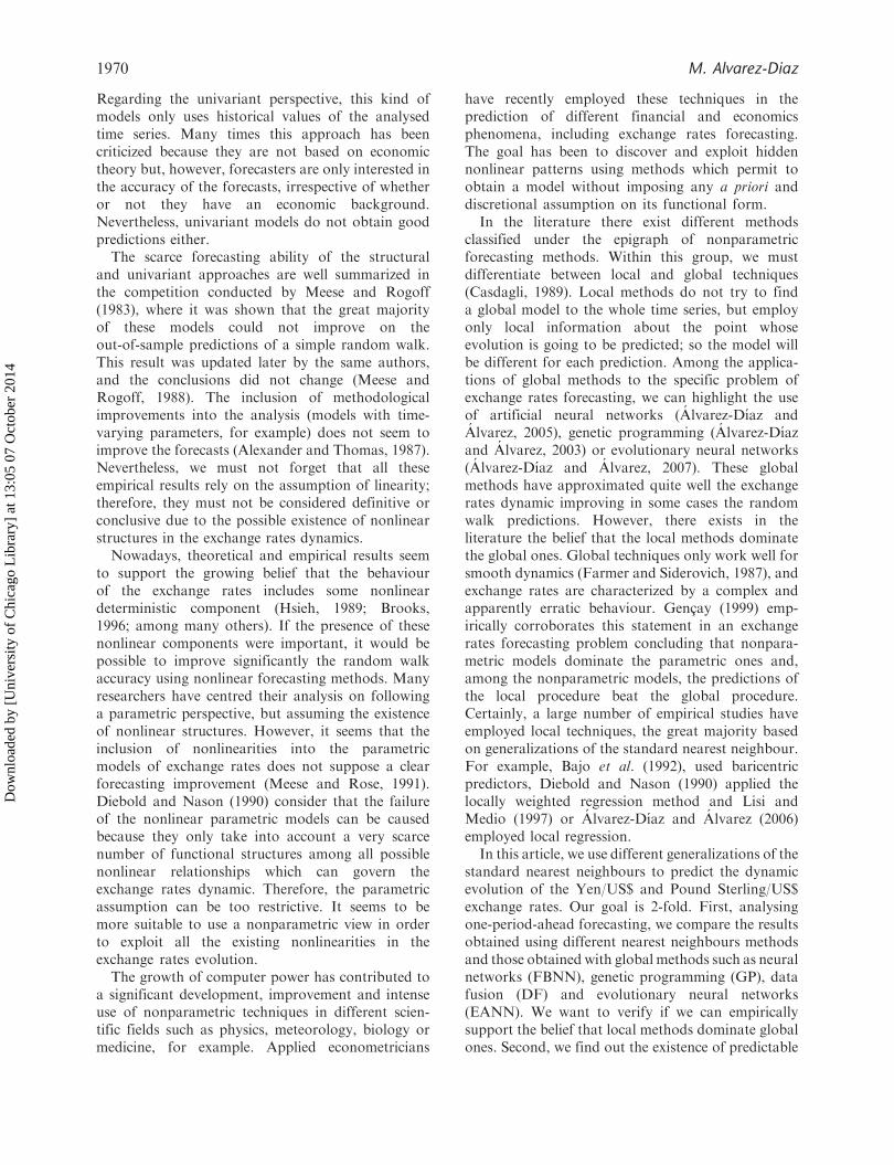
Regarding the univariant perspective, this kind ofmodels only uses historical values of the analysedtime series. Many times this approach has beencriticized because they are not based on economictheory but, however, forecasters are only interested inthe accuracy of the forecasts, irrespective of whetheror not they have an economic background.Nevertheless, univariant models do not obtain goodpredictions either.

The scarce forecasting ability of the structuraland univariant approaches are well summarized inthe competition conducted by Meese and Rogoff(1983), where it was shown that the great majorityof these models could not improve on theout-of-sample predictions of a simple random walk.This result was updated later by the same authors,and the conclusions did not change (Meese andRogoff, 1988). The inclusion of methodologicalimprovements into the analysis (models with time-varying parameters, for example) does not seem toimprove the forecasts (Alexander and Thomas, 1987).Nevertheless, we must not forget that all theseempirical results rely on the assumption of linearity;therefore, they must not be considered definitive orconclusive due to the possible existence of nonlinearstructures in the exchange rates dynamics.

Nowadays, theoretical and empirical results seemto support the growing belief that the behaviourof the exchange rates includes some nonlineardeterministic component (Hsieh, 1989; Brooks,1996; among many others). If the presence of thesenonlinear components were important, it would bepossible to improve significantly the random walkaccuracy using nonlinear forecasting methods. Manyresearchers have centred their analysis on followinga parametric perspective, but assuming the existenceof nonlinear structures. However, it seems that theinclusion of nonlinearities into the parametricmodels of exchange rates does not suppose a clearforecasting improvement (Meese and Rose, 1991).Diebold and Nason (1990) consider that the failureof the nonlinear parametric models can be causedbecause they only take into account a very scarcenumber of functional structures among all possiblenonlinear relationships which can govern theexchange rates dynamic. Therefore, the parametricassumption can be too restrictive. It seems to bemore suitable to use a nonparametric view in orderto exploit all the existing nonlinearities in theexchange rates evolution.

The growth of computer power has contributed toa significant development, improvement and intenseuse of nonparametric techniques in different scien-tific fields such as physics, meteorology, biology ormedicine, for example. Applied econometricians

have recently employed these techniques in theprediction of different financial and economicsphenomena, including exchange rates forecasting.The goal has been to discover and exploit hiddennonlinear patterns using methods which permit toobtain a model without imposing any a priori anddiscretional assumption on its functional form.

In the literature there exist different methodsclassified under the epigraph of nonparametricforecasting methods. Within this group, we mustdifferentiate between local and global techniques(Casdagli, 1989). Local methods do not try to finda global model to the whole time series, but employonly local information about the point whoseevolution is going to be predicted; so the model willbe different for each prediction. Among the applica-tions of global methods to the specific problem ofexchange rates forecasting, we can highlight the useof artificial neural networks (Alvarez-Dıaz andAlvarez, 2005), genetic programming (Alvarez-Dıazand Alvarez, 2003) or evolutionary neural networks(Alvarez-Dıaz and Alvarez, 2007). These globalmethods have approximated quite well the exchangerates dynamic improving in some cases the randomwalk predictions. However, there exists in theliterature the belief that the local methods dominatethe global ones. Global techniques only work well forsmooth dynamics (Farmer and Siderovich, 1987), andexchange rates are characterized by a complex andapparently erratic behaviour. Gencay (1999) emp-irically corroborates this statement in an exchangerates forecasting problem concluding that nonpara-metric models dominate the parametric ones and,among the nonparametric models, the predictions ofthe local procedure beat the global procedure.Certainly, a large number of empirical studies haveemployed local techniques, the great majority basedon generalizations of the standard nearest neighbour.For example, Bajo et al. (1992), used baricentricpredictors, Diebold and Nason (1990) applied thelocally weighted regression method and Lisi andMedio (1997) or Alvarez-Dıaz and Alvarez (2006)employed local regression.

In this article, we use different generalizations of thestandard nearest neighbours to predict the dynamicevolution of the Yen/US$ and Pound Sterling/US$exchange rates. Our goal is 2-fold. First, analysingone-period-ahead forecasting, we compare the resultsobtained using different nearest neighbours methodsand those obtained with global methods such as neuralnetworks (FBNN), genetic programming (GP), datafusion (DF) and evolutionary neural networks(EANN). We want to verify if we can empiricallysupport the belief that local methods dominate globalones. Second, we find out the existence of predictable

1970 M. Alvarez-Diaz

Dow

nloa

ded

by [

Uni

vers

ity o

f C

hica

go L

ibra

ry]

at 1

3:05

07

Oct

ober

201

4

structures � periods ahead in the considered exchange

rates.

This article is structured in five sections. After

this introductory section, the different nearest

neighbours methods are explained. In Section III,

the data are described and some technical details are

explained. In Section IV, the results obtained for each

local method are showed, commented and compared

with the global ones. Lastly, we conclude with a

summary of the main findings and results.

II. Nearest Neighbour Methods

The nearest neighbour method (NN) is one of the

nonparametric techniques most widely used for

nonlinear financial prediction and, specifically, for

exchange rates forecasting (Diebold and Nason,

1990). Basically, two reasons can explain this fact.

First, the computational requirements are not as high

as other methods such as neural networks or genetic

programming and, second, they have empirically

shown an important forecasting capacity. The

method is inspired by the predictions of nonlinear

dynamic systems (Farmer and Siderowich, 1987),

and seeks to predict the future dynamics of a time

series by analysing how it has evolved in similar

situations in the past before. Therefore, forecasters

only take the most recent history available and search

over the past dynamics the K most similar patterns,

called the nearest neighbour vectors. Later on, they

analyse toward which values these past dynamics

have evolved and, using this information, they infer

toward which value the most recent history is likely

going to evolve.In our application, we use different generalizations

of the method. To be more specific, we employ

different schemes of baricentric predictors and local

regression (Cleveland and Devlin, 1988). Every

method differs from other only in certain technical

details, but there exists a common procedure for all

of them which can be briefly described by a series

of simple steps. First of all, given a time series fxtgTt¼1,

the following matrix is constructed

which is called the Trajectory Matrix. Each rowof the trajectory matrix is made up of vectors of thefollowing form

Xi ¼ ðxi, xiþ�, xiþ2�, . . . , xiþðm�1Þ�Þ

i ¼ 1, . . . ,T� �ðm� 1Þ ð2Þ

defining a vector space whose dimension (m) is calledembedding dimension and � is known as the delayparameter. According to the Takens’ Theorem (1981),the geometrical trajectory of this sequence of vectorsforms a multi-dimensional object at <m whichmaintains unaltered certain characteristics of thetrue but unknown process that generates the data,for appropriate values of m and �. Furthermore,if the time series is deterministic, the Theoremguarantees the possibility of predicting its evolutionfrom past values.

One important question is how to find appropriatevalues for the embedding dimension and time delay.There is a large literature on the optimal choice ofthese parameters. For the delay choice, we can finddifferent procedures to choose � from a time seriessuch as the autocorrelation function method and themutual information method (Fraser and Swinney,1986), however, they are not considered too rigorous.In our study, we shall only consider the case of �¼ 1.Three reasons justified our choice: we simplify ouranalysis without excessively modifying the finalresult, we reduce the computational time and, finally,this assumption is employed in the majority of theforecasting studies in Finance (Fernandez-Rodrıguezet al., 1999) and, specifically, in exchange ratesforecasting (Bajo-Rubio et al., 1992; Soofi and Cao,1999). Regarding to the optimal choice of theembedding dimension, we can also find in theliterature different methods which help to select m,but neither of them is accepted by general consensusamong researchers. For example, the method of falsenearest neighbours provides one of the most employedpossibility for estimating m (Kennel et al., 1992);however, arbitrary parameters must be previouslyestablished by the researcher. In our specific

�T�ðm�1Þ�xm ¼

X1

X2

:

:

:

XT��ðm�1Þ

0BBBBBBBB@

1CCCCCCCCA¼

x1 x1þ� : : : x1þðm�1Þ�

x2 x2þ� : : : x2þðm�1Þ�

: : : : : :

: : : : : :

: : : : : :

xT�ðm�1Þ� xT�ðm�1Þ�þ� : : : xT

0BBBBBBBB@

1CCCCCCCCA

ð1Þ

Exchange rates forecasting 1971

Dow

nloa

ded

by [

Uni

vers

ity o

f C

hica

go L

ibra

ry]

at 1

3:05

07

Oct

ober

201

4

forecasting study, we adopt a trial-and-error proce-

dure in order to select m (Casdagli, 1992). We will

pick up the thread before finishing this section where

a more detailed explanation about the choice of this

parameter will be offered.Given the common assumption of �¼ 1, the

Trajectory Matrix will adopt the form

�T�mþ1xm ¼

X1

X2

:

:

:

XT�mþ1

0BBBBBBBBB@

1CCCCCCCCCA

¼

x1 x2 : : : xm

x2 x3 : : : xmþ1

: : : : : :

: : : : : :

: : : : : :

xT�mþ1 xT�mþ2 : : : xT

0BBBBBBBBB@

1CCCCCCCCCAð3Þ

The following step consists in specifying toward

which value has evolved each Xi vector

ð8i ¼ 1, . . . ,T�m� � þ 1Þ� periods ahead. To do

so, the Evolution Matrix is constructed:

EðT�m��þ1Þxðmþ1Þ

¼

X1

X2

:

:

:

XT�m��þ1

R1

R2

:

:

:

RT�m��þ1

��

0BBBBBBBBB@

1CCCCCCCCCA

¼

x1 x2 : : : xm

x2 x3 : : : xmþ1

: : : : : :

: : : : : :

: : : : : :

xT�m��þ1 xT�m��þ2 : : : xT��

xmþ�

xmþ1þ�

:

:

:

xT

��

0BBBBBBBBB@

1CCCCCCCCCAð4Þ

where the last column shows the value generated

by the vector Xi � periods in the future. For example,

the vector X1 ¼ ðx1, x2, . . . , xmÞ has generated a

future value R1 ¼ xmþ� and the vector XT�m��þ1 ¼

ðxT�m��þ1, xT�m��þ2, . . . , xT��Þ has given a future

value RT�m��þ1 ¼ xT. Once the trajectory matrix

has been defined, the next step is to select the past

dynamics which are more similar to the recent

behaviour of the time series (XT�mþ1). To do so, we

look for the K vectors Xi 2 <m which minimize the

distance regarding to XT�mþ1. Different concepts

of distance have been recommended in the literature.

Casdagli (1989) suggests employing the sup norm to

calculate distances, while others advocate the use

of the Euclidean norm (Yakowitz, 1987, Cleveland

and Devlin, 1988). We consider the last recommenda-

tion given its widespread use in forecasting exchange

rates. In formal notation, the K closest neighbours

to the current dynamic XT�mþ1 will be the vectors

which minimize the function.

di ¼ distaðXi,XT�mþ1Þ ¼ Xi � XT�mþ1��

¼Xml¼1

xl, 1 � xl,T�mþ1� �2� � !1=2

ð5Þ

Therefore, based on the calculation of the Euclidean

distance, we can build both the N matrix with the

K vectors closest to XT�mþ1, as well as the E matrix

which reflects the value to which each of the K vectors

evolves � period ahead.

NKxðmþ1Þ ¼

N1

N2

:

:

:

NK

0BBBBBBBBBB@

1CCCCCCCCCCA¼

k11 k12 : : : k1m

k21 k22 : : : k2m

: : : : : :

: : : : : :

: : : : : :

kK1 kK2 : : : kkm

0BBBBBBBBBB@

1CCCCCCCCCCA

;

EKx1 ¼

E1

E2

:

:

:

EK

0BBBBBBBBBB@

1CCCCCCCCCCA

ð6Þ

For example, the vector N1 has evolved to a value

E1 at � periods in the future, while the vector NK has

generated a value EK. Each vector Ni inside this

matrix is sorted according to its distance to XT�mþ1.

In this way, N1 and NK are the closest and the more

distant vectors to XT�mþ1, respectively.Up to this point the common procedure for the

different nearest neighbour methods has been

described. How to predict the future value xTþ�from the recent history XT�mþ1 will make the

difference among the methods. We start with

the easiest and simplest method of local prediction:


Dow

nloa

ded

by [

Uni

vers

ity o

f C

hica

go L

ibra

ry]

at 1

3:05

07

Oct

ober

201

4

the nearest neighbour method (Lorenz, 1969).

This method considers as predictor exclusively the

evolution of the closest point N1 (the nearest

neighbour)

xTþ� ¼ E1 ð7Þ

This simple method is very intuitive, didactic and it

does not require excessive time computing. However,

we exclude it in our study because for short and/or

noisy time series this method has a scarce forecasting

power. An improvement is simply to take the average

of the K nearest neighbours (unweighted baricentric

predictor)

xTþ� ¼E1 þ E2 þ � � � þ EK

Kð8Þ

or the average can be also weighted according to the

distance of the respective nearest neighbour points

to the target point XT�mþ1 (weighted baricentric

predictor)

xTþ� ¼ w1 � E1 þ w2 � E

2 þ � � � þ wK � EK ð9Þ

where

wi ¼distaðXi,XT�mþ1ÞXK

j¼1distaðXj,XT�mþ1Þ

ð10Þ

This is only one of a number of plausible weight

functions that one might choose but, from a

computational point of view, this structure of

weighting is the most popular in literature. Another

generalization is to assume a first order or linear

approximation taking the K nearest neighbours and

fitting a linear polynomial (local regression)

xTþ� ¼ b0 þ b1 � xT�mþ1 þ b2 � xT�mþ2 þ � � �

þ bm � xT ð11Þ

where the coefficients bi are estimated by ordinary

least squares (OLS), using the matrices N and E

(b ¼ ðN0NÞ�1N0E).Other more complex alternatives of local regression

include different weighting schemes (weighted local

regression). We can mention the use of the tricube

function (Diebold and Nason, 1990)

ui ¼ ð1� w3i Þ

3ð12Þ

with

wi ¼distaðXi,XT�mþ1Þ

distaðXK,XT�mþ1Þð13Þ

or the exponential weight function

ui ¼ expð�distaðXi,XT�mþ1ÞÞ ð14Þ

These structures produce a smooth and gradualdecline in weights regarding to the distance fromXT�mþ1. Considering these weighting procedures, theN and E matrices will adopt the form

N�Kxðmþ1Þ ¼

N�1

N�2

:

:

:

N�K

0BBBBBBBB@

1CCCCCCCCA

¼

u1 � k11 u1 � k12 : : : u1 � k1m

u2 � k21 u2 � k22 : : : u2 � k2m

: : : : : :

: : : : : :

: : : : : :

uk � kK1 uk � kK2 : : : uk � kkm

0BBBBBBBB@

1CCCCCCCCA

;

E�K�1 ¼

u1 � E1

u2 � E2

:

:

:

uk � EK

0BBBBBBBB@

1CCCCCCCCA

ð15Þ

And the predictions will arrive from the expression

xTþ� ¼ b�0 þ b�1 � xT�mþ1 þ b�2 � xT�mþ2 þ � � �

þ b�m � xT ð16Þ

where the coefficients b�i are estimated by OLS,employing now the matrices N* and E*(b� ¼ ðN�0N�Þ�1N� 0E�). The weighted local regressionshows certain attractive theoretical aspects but,empirically, there exist difficulties in its implementa-tion and, in presence of noise, it provides very oftenworse predictions than unweighted local regression(Jaditz and Riddick, 2000).

Once the common procedure and the differentapproaches of predicting have been detailed, it stillremains the problem of selecting the optimal values ofm and K. The success of the prediction dependsdeeply on the right choice of these parameters.Regarding K, there is no general guideline forchoosing this parameter which has been generallyaccepted among researchers. Some basic recommen-dations have been proposed in the literature likesetting K � 2 � ðmþ 1Þ (Casdagli, 1989), or K ¼ T�

with �<1 (Diebold and Nason, 1990), but theymust be set up discretionally. Following the recom-mendations proposed in the literature, we select Kand m at the same time using a trial-and-error process(Casdagli, 1992). Therefore, we try with different


Dow

nloa

ded

by [

Uni

vers

ity o

f C

hica

go L

ibra

ry]

at 1

3:05

07

Oct

ober

201

4

values of K and m, and we choose such combinationwhich optimizes a given fit criterion in a specificsub-sample (called selection period). We assumethe specific framework developed by Hsieh (1991)analysing a number of nearest neighbour between10% of all observations up to 90%, increasing insteps of 10% and, for the case of the embeddingdimension, we consider values from two to ten.

III. Data and Forecasting Set Up

Our database is composed of weekly data on theexchange rates for the Japanese Yen and the PoundSterling against the American Dollar, and it wasdownloaded from The Pacific Exchange RatesService (University of British Columbia). Thesecurrencies along with the Euro conform the corecurrencies in the world economy. The weekly data isthe exchange rate during a representative day of theweek, usually Wednesday, and if a particularWednesday happens to be a nontrading day,then either Tuesday or Thursday are retained(Diebold and Nason, 1990). The sample finallyselected goes from the first week of 1973 to the lastweek of July 2002; therefore, a total of 1542 areobtained. A weekly frequency avoids possible biasesinherent to daily data (weekend effect, for example)and, moreover, it contains sufficient informationto reflect accurately the dynamics of exchangerates (Yao and Tan, 2000). As usual in financialforecasting and, specifically, in exchange rates fore-casting, we consider the difference of the exchangerate logarithm,

xt ¼ logðytÞ � logðyt�1Þ ð17Þ

where yt is the exchange rate under analysis, log (yt)is its logarithmic transformation and xt its return.This transformation has become standard in financialanalyses as it allows us to obtain a stationary seriesthat can be interpreted as returns. However, takingdifferences can increase the existing noise in the seriesand, in consequence, destroy some predictable signal(Broomhead and King, 1988; Soofi and Cao, 1999).If we assumed the academic postulates and weconsidered that the exchange rates followed arandom walk process, the sequence fxtg

Tt¼1 would be

random and unpredictable. There would not be anychance of obtaining accurate predictions employingany kind of forecasting methods.

In order to achieve a fair predictive exercise andfollowing the recommendations proposed in thespecialized literature (Yao and Tan, 2000), the totalsample was divided into three sub-periods: Training,

selection and out-of-sample. The first one, composedby the first 1080 observations, is reserved as historyof the time series. The selection period, which coversthe 306 following observations, is used to determinean optimal value for the parameters m and K. Finally,we have reserved the last 155 observations to validatethe predictive ability of the methods.

In this specific forecasting study, we will applytwo kinds of fit criterions depending if we wantto predict the exact value of the exchange rate(point prediction), or if we want to anticipate thedirection of its sign movements (sign prediction).For the point prediction, we consider as fit criterionthe Normalized Mean Square Error (NMSE) definedby the expression

NMSE ¼1

VarðxÞ�

XM

t¼mþ1xt � xt½ �

2

Tsð18Þ

where Var(x) is the variance of the time series,Ts is the total number of observations in the specificsub-sample S, and xt and xt are the predicted andactual value, respectively. This fit criterion comparesthe errors of the forecasting method and the errorsobtained by considering the sample mean as naivepredictor. Therefore, a NMSE value lower/equal/higher than one would imply a forecasting abilitybetter than/equal to/worse than the mean aspredictor. The criterion has been recommended inthe literature (Casdagli, 1989) and it was used toevaluate entries into the Santa Fe Time SeriesCompetition (Weigend and Gershenfeld, 1992).Moreover, the measure has been traditionally appliedin exchange rate forecasting (Elms, 1994; Tenti, 1996;Yao et al., 1999; Yao and Tan, 2000).

On the other hand, for the sign prediction, the fitcriterion will be the success ratio defined by theexpression

SR ¼

XM

t¼mþ1�½xt � xt > 0�

Tsð19Þ

where SR is the ratio of correctly predicted signs(success ratio) and �ð�Þ is the Heaviside function(�ð�Þ ¼ 1 if xt � xt > 0 and �ð�Þ ¼ 0 if xt � xt < 0).Therefore, this criterion gives us the percentage ofcorrect predictions in direction changes.

IV. Results

Point predictions

Analysing one-period-ahead forecasts, Figs 1 and 2show the sensitivity of the considered nearestneighbour methods to different embedding


Dow

nloa

ded

by [

Uni

vers

ity o

f C

hica

go L

ibra

ry]

at 1

3:05

07

Oct

ober

201

4

Fig. 1. Point prediction: selection of the embedding dimension: YEN/$ case. (a) Unweighted baricentric predictor; (b) Weighted

baricentric predictor; (c) Local regression; (d) Tricube weighted local regression; (e) Exponential weighted local regression


Dow

nloa

ded

by [

Uni

vers

ity o

f C

hica

go L

ibra

ry]

at 1

3:05

07

Oct

ober

201

4

Fig. 2. Selection of the embedding dimension: BP/$ case. (a) Unweighted baricentric predictor; (b) Weighted baricentric

predictor; (c) Local regression; (d) Tricube weighted local regression; (e) Exponential weighted local regression


Dow

nloa

ded

by [

Uni

vers

ity o

f C

hica

go L

ibra

ry]

at 1

3:05

07

Oct

ober

201

4

dimensions in terms of the NMSE reached in theselection sample. As we can observe, all methodsshow a smooth predictive behaviour consideringdifferent delays. In spite of this stability andfollowing the trial-and-error process previously com-mented, we have chosen the value of the embeddingdimension (m) which minimizes the NMSE in theselection period.

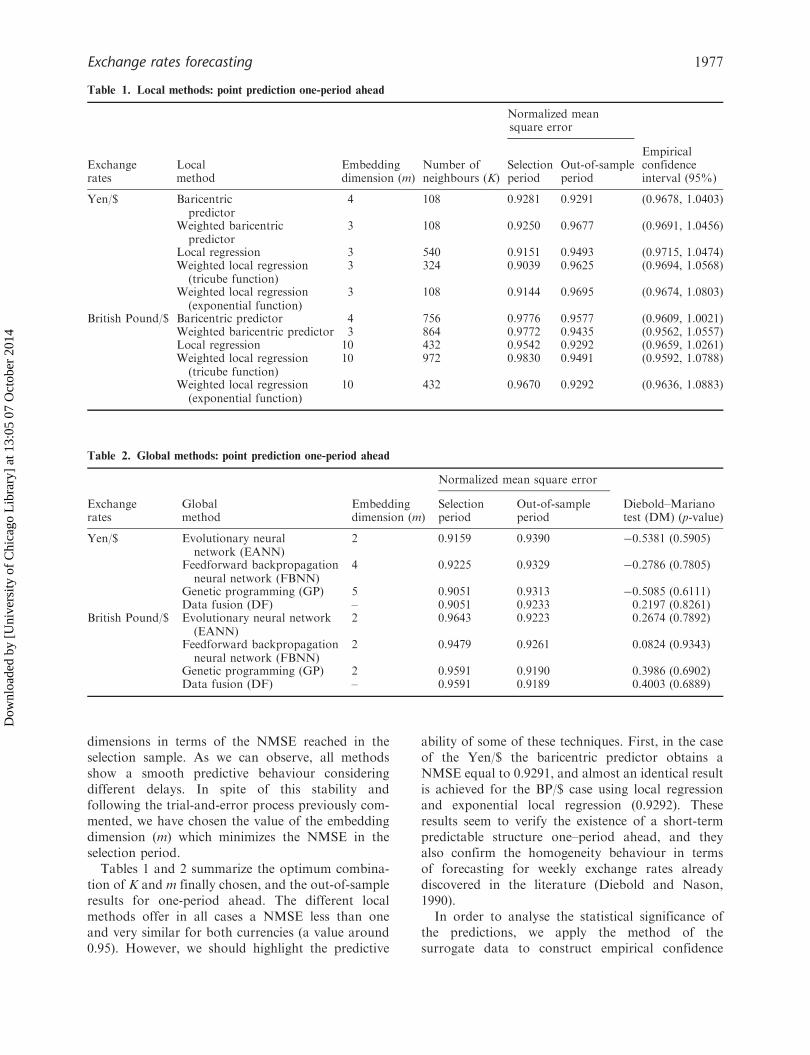
Tables 1 and 2 summarize the optimum combina-tion of K and m finally chosen, and the out-of-sampleresults for one-period ahead. The different localmethods offer in all cases a NMSE less than oneand very similar for both currencies (a value around0.95). However, we should highlight the predictive

ability of some of these techniques. First, in the caseof the Yen/$ the baricentric predictor obtains aNMSE equal to 0.9291, and almost an identical resultis achieved for the BP/$ case using local regressionand exponential local regression (0.9292). Theseresults seem to verify the existence of a short-termpredictable structure one–period ahead, and theyalso confirm the homogeneity behaviour in termsof forecasting for weekly exchange rates alreadydiscovered in the literature (Diebold and Nason,1990).

In order to analyse the statistical significance ofthe predictions, we apply the method of thesurrogate data to construct empirical confidence

Table 2. Global methods: point prediction one-period ahead

Normalized mean square error

Exchangerates

Globalmethod

Embeddingdimension (m)

Selectionperiod

Out-of-sampleperiod

Diebold–Marianotest (DM) (p-value)

Yen/$ Evolutionary neuralnetwork (EANN)

2 0.9159 0.9390 �0.5381 (0.5905)

Feedforward backpropagationneural network (FBNN)

4 0.9225 0.9329 �0.2786 (0.7805)

Genetic programming (GP) 5 0.9051 0.9313 �0.5085 (0.6111)Data fusion (DF) – 0.9051 0.9233 0.2197 (0.8261)

British Pound/$ Evolutionary neural network(EANN)

2 0.9643 0.9223 0.2674 (0.7892)


2 0.9479 0.9261 0.0824 (0.9343)

Genetic programming (GP) 2 0.9591 0.9190 0.3986 (0.6902)Data fusion (DF) – 0.9591 0.9189 0.4003 (0.6889)

Table 1. Local methods: point prediction one-period ahead

Normalized meansquare error

Exchangerates

Localmethod


Number ofneighbours (K)

Selectionperiod

Out-of-sampleperiod

Empiricalconfidenceinterval (95%)

Yen/$ Baricentricpredictor

4 108 0.9281 0.9291 (0.9678, 1.0403)

Weighted baricentricpredictor

3 108 0.9250 0.9677 (0.9691, 1.0456)

Local regression 3 540 0.9151 0.9493 (0.9715, 1.0474)Weighted local regression(tricube function)

3 324 0.9039 0.9625 (0.9694, 1.0568)

Weighted local regression(exponential function)

3 108 0.9144 0.9695 (0.9674, 1.0803)

British Pound/$ Baricentric predictor 4 756 0.9776 0.9577 (0.9609, 1.0021)Weighted baricentric predictor 3 864 0.9772 0.9435 (0.9562, 1.0557)Local regression 10 432 0.9542 0.9292 (0.9659, 1.0261)Weighted local regression(tricube function)

10 972 0.9830 0.9491 (0.9592, 1.0788)


10 432 0.9670 0.9292 (0.9636, 1.0883)


Dow

nloa

ded

by [

Uni

vers

ity o

f C

hica

go L

ibra

ry]

at 1

3:05

07

Oct

ober

201

4

intervals (Theiler et al., 1992). This method hasbecome a very useful analytical tool for manyscientific fields, including finance. The proceduresimply implies a permutation of data, and it can beeasily explained as follows. We artificially generate1.000 time series randomly shuffling the originaldata. By scrambling the data, we should destroy anypossible deterministic structure, but we maintainthe distributional properties of the original series.Later on, we apply our local methods to theseartificial and random series, we calculate theircorresponding NMSE and, finally, we construct anempirical distribution. If there were no predictablestructures, the NMSE obtained in the original seriesshould not be statistically different than the NMSEobtained by the shuffled series. Using the empiricaldistribution of NMSE, we can build a confidenceinterval with a specific significant level, in our caseat the 95%. Any NMSE inside this empiricalinterval would be considered as the result of theapplication of a forecasting method on a randomand unpredictable time series. Tables 1 and 2 alsoshows the empirical confidence interval at 95% forthe predictions of Yen/US$ and Pound Sterling/US$, respectively. We can observe how the totalityof the NMSE is out of the empirical intervalallowing us to verify statistically the existence ofpredictable structures in the exchange rate evolution.

In order to reaffirm the discovery of thesepredictable nonlinear structures, we follow theapproach introduced by Sugihara and May (1990)and empirically applied in economics by Finkenstadtand Kuhbier (1995) and Agnon et al. (1999), amongothers. The basic procedure consists on analysing theforecasting accuracy evolution of a time series.Specifically, for an unpredictable time series, theaccuracy of applying a nonlinear forecastmethod must wander around a NMSE equal to one(the accuracy of applying the mean as naıvepredictor) when increasing the forecast horizon.However, if the existence of short nonlinear pre-dictable dynamics was important, we should observethat the accuracy of the nonlinear forecast falls offwhen increasing the prediction period. In our study,Fig. 3 shows how the most accurate predictions forthe whole methods is achieved for one-period aheadand, for more periods ahead, the out-of-sampleNMSE increases and fluctuates around one.Therefore, this result seems to corroborate theexistence of a slightly but significant short-termpredictable pattern in the studied exchange ratesreturns.

Table 2 depicts the results previouslyobtained using global methods: a feedforwardbackpropagation neural network (FBNN), a genetic

programming (GP), data fusion (DF) (Alvarez-Dıazand Alvarez, 2005) and an evolutionary neuralnetwork (EANN) (Alvarez-Dıaz and Alvarez,2007). The comparison shows that all these globalmethods exploit the existing predictable nonlinearity,and all of them obtain similar forecastingresults to local methods. To be more precise, in thecase of Yen/US$, the baricentric predictor (0.9291)beats all global methods except data fusion (0.9233).However, for the Pound Sterling/US$ case, wecannot find a local method which improves anyof the global methods. Table 2 also providesinformation about the Diebold–Mariano Test. Theuse of this test in our application attempts to verifyif the predictions of the best local method (baricentricand local regression for Yen/US$ and PoundSterling/US$, respectively) are statistically differentthan those obtained using global techniques.Diebold and Mariano (1994) show that, underthe null hypothesis of equal forecasts ability

Fig. 3. Point prediction to different periods. (a) Yen /$

exchange rate; (b) BP/$ exchange rate


Dow

nloa

ded

by [

Uni

vers

ity o

f C

hica

go L

ibra

ry]

at 1

3:05

07

Oct

ober

201

4

between methods ðH0 : E ½ðerrorBest Local Methodtþ1 Þ

2� ¼

E½ðerrorGlobal Methodtþ1 Þ

2�Þ, the following statistic follows

asymptotically a standard normal distribution

D�M Test ¼�dffiffiffiffiffiffiffiffiffiffiffiffiffiffiffiffiffiffiffiffiffiffi

2� fdð0Þ=H

q ð20Þ

where H is the out-of-sample size, fdð0Þ is a consistent

estimate of the spectral density of the loss differential

at frequency zero corrected for serial correlation and

�d ¼

PðerrorGlobal Method

tþ1 Þ2� ðerrorBest Local Method

tþ1 Þ2

� H

ð21Þ

is the sample mean loss differential. A negative and

statistically significant value of the D–M test would

imply to reject the null hypothesis and, in conse-

quence, we could assert that the best local method

provides statistically better predictions that the

considered global method. However, observing

the D–M Test in Table 2 for both currencies and

for the different global methods, we can verify that

there are no statistical differences between the best

nearest neighbour and the rest of the global methods.

Therefore, we cannot generalize the deeply rooted

belief that local methods beat global ones in a

forecasting exchange rate exercise (Gencay, 1999).

In our specific predictive exercise, we verify that the

local methods offer statistically similar results than

the global ones.

Sign prediction

In this section our goal is to anticipate the direction

in which the exchange rate will move. Instead

of forecasting the exact value of the exchange rate,

now we centre our analysis on trying to forecast

whether there will be a currency appreciation or

depreciation. For empirical financial purposes, this

kind of analysis is much more interesting than point

prediction because even the smallest forecast errors

can lead to heavy losses in capital if the direction

of the forecast is mistaken (Tenti, 1996; Lisi and

Medio, 1997).Similar to the case of point prediction one-period

ahead, Figs 4 and 5 show the relative stability of the

success ratio in the selection period when different

embedding dimensions are considered. Again, follow-

ing our analytical procedure, we have selected the

value of m which optimizes the fit criterion in a

specific sub-sample. Therefore, we have chosen the

embedding dimension with the highest percentage

of correctly predicted signs in the selection period.

Table 3 shows the optimal combination of mand K, and the selection and out-of-sample successratio for each local method and for each analysedexchange rate. Regarding to the dynamics of the Yen/US$ exchange rate, the highest percentage is obtainedusing local regression and tricube local regression(58.33%). Applying once more the Surrogate method,we observe how almost the totality of the obtainedsuccess ratios is outside of the empirical interval.For the Pound Sterling/US$ exchange rates, thebest results are now obtained employing weightedbaricentric predictor and tricube local regression(57.69%). As before, the majority of the percentagesare outside of the empirical interval confirmingthe statistical significance of our predictions and,in consequence, allowing us to reject any randomnessin the dynamics of the analysed exchange rates.Therefore, these results are better than pure chance at5% significance level. Our results of one-period aheadalso state the great difficulty existing in exchangerates forecasting in exceeding the threshold of 60%(Lequarre, 1993).

Table 4 depicts the success ratios using globalmethods. The comparison among methods allows usto verify the forecasting superiority of global methodsin terms of directional accuracy. For both currencies,only in two cases the local methods outperformglobal methods (neural networks and evolutionaryneural networks, both cases for the Pound Sterling/US$ exchange rate). Therefore, for sign prediction weprove again the nonsuperiority of local methods.

Figure 6 describes the results obtained consideringdifferent prediction periods for the Yen/US$ andPound Sterling/US$. The analysis ofthis figure provides new evidences against theunpredictability of the exchange rates evolution. Ifthe time series was unpredictable, one would expectto observe a fluctuation in the percentage of correctforecasts about 50% (predictions obtained throwinga coin). However, we observe again how the highestpercentage is obtained one-period ahead and,when more predictive periods are considered, theforecasting ability is lost. This finding suggestsagain the existence of a predictive power which islimited only to the immediate future.

V. Conclusion

In this article, we have used different generalizationsof the standard nearest neighbours to predict thedynamic evolution of the Yen/$ and BP/$ exchangerates. Our results corroborate certain stylized factsin exchange rates forecasting. First, we confirm thehomogeneous behaviour in terms of forecasting


Dow

nloa

ded

by [

Uni

vers

ity o

f C

hica

go L

ibra

ry]

at 1

3:05

07

Oct

ober

201

4

Fig. 4. Sign prediction: Selection of the embedding dimension: YEN/$ Case. (a) Unweighted baricentric predictor; (b) Weightedbaricentric predictor; (c) Local regression; (d) Tricube weighted local regression; (e) Exponential weighted local regression


Dow

nloa

ded

by [

Uni

vers

ity o

f C

hica

go L

ibra

ry]

at 1

3:05

07

Oct

ober

201

4

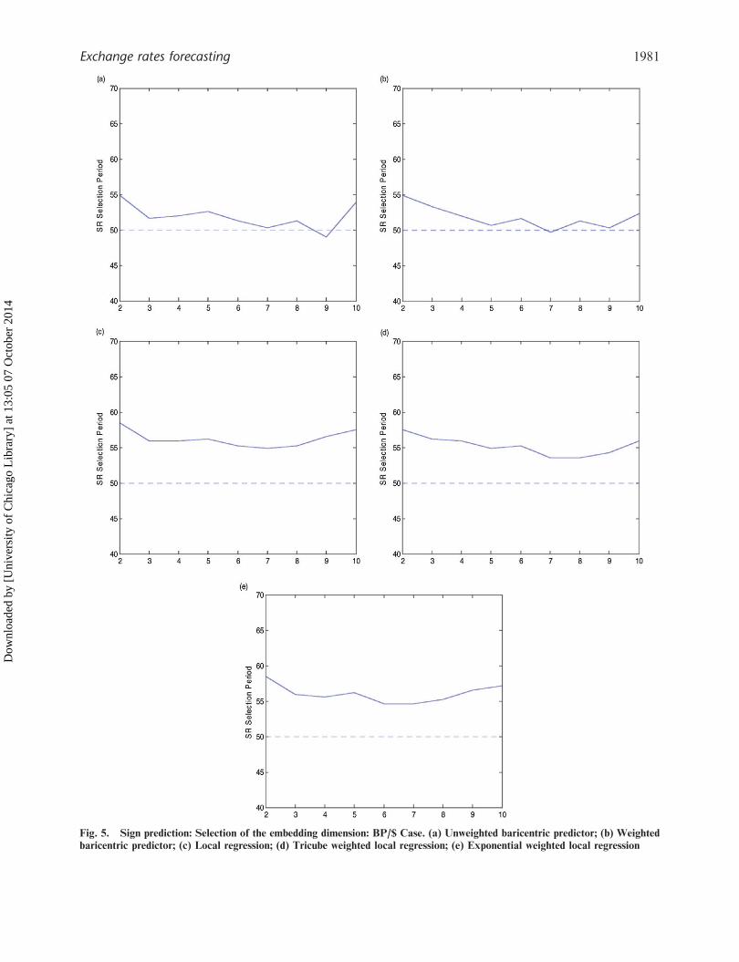
Fig. 5. Sign prediction: Selection of the embedding dimension: BP/$ Case. (a) Unweighted baricentric predictor; (b) Weighted

baricentric predictor; (c) Local regression; (d) Tricube weighted local regression; (e) Exponential weighted local regression


Dow

nloa

ded

by [

Uni

vers

ity o

f C

hica

go L

ibra

ry]

at 1

3:05

07

Oct

ober

201

4

for weekly exchange rate returns previously described

by Diebold and Nason (1990). Second, we verify the

existence of a significant short-term predictable

structure in the temporal evolution of both curren-

cies. We can obtain accurate predictions one-period

ahead, but this predictive capacity is lost when more

periods ahead are considered. Third, we also verify in

sign prediction the difficulties to exceed the 60%

threshold reported in the literature. Besides verifying

these stylized facts, our results do not confirm thegeneral belief which states that local methods

dominate the global ones in an exchange rates

forecasting exercise. At least for our specific applica-

tion, we could not find statistical predictive differ-

ences between both kinds of methods. Even more,

many times global techniques offered better predic-

tive results in terms of point and sign prediction.In summary, our predictive exercise provides

evidences against the unpredictability of the exchange

rates dynamic and, in consequence, against thestatement that exchange rates follow a random walk

process. Considering both point prediction and sign

prediction, the local and global methods offer

statistically significant better predictions than the

random walk model. However, in spite of this

significant improvement, the predictive gain is

small. We have obtained a NMSE around 0.93 and

a success ratio less than 60%. In the literature, we can

find several possible explanations to this significant

but poor predictability. First of all, it is possible theexistence of a weak nonlinear deterministic structure

in exchange rates, but we cannot exploit it to get a

great forecasting improvement (Diebold and Nason,

Table 3. Local methods: sign prediction one-period ahead

Success ratio

Exchangerates

Localmethod


Number ofneighbours (K)

Selectionperiod

Out-of-sampleperiod

Empiricalconfidenceinterval (95%)

Yen/$ Baricentric predictor 3 432 60.46 55.77 (41.67, 51.28)Weighted baricentric

predictor3 216 59.15 53.21 (40.38, 53.85)

Local regression 9 648 61.11 58.33 (40.38, 55.77)Weighted local regression

(tricube function)3 216 59.80 53.85 (40.38, 55.77)


9 648 61.44 58.33 (41.06, 56.41)

British Pound/$ Baricentric predictor 2 108 54.9 56.44 (42.31, 57.69)Weighted baricentric predictor 2 108 54.9 57.69 (41.67, 56.41)Local regression 2 540 58.5 56.77 (41.94, 56.77)Weighted local regression

(tricube function)2 108 57.52 57.69 (42.31, 57.05)


2 540 58.5 56.41 (42.31, 56.41)

Fig. 6. Sign prediction to different periods. (a) Yen/$

exchange rate; (b) BP/$ exchange rate


Dow

nloa

ded

by [

Uni

vers

ity o

f C

hica

go L

ibra

ry]

at 1

3:05

07

Oct

ober

201

4

1990). Another possible explanation would be thatwe need the development and/or improvement ofthe forecasting techniques. One final explanation,suggested by Stengos (1996), could be that, due to thegreat complexity present in the financial market(probably chaotic), an accurate forecast analysiswould require an extremely high number of observa-tions. Nevertheless, exchange rates forecasting is stillan open research avenue and more efforts must berealized in order to reach more accurate predictions.

Acknowledgements

I wish to thank Ministerio de Educacion y Ciencia

(Grant MTM2005-01274, FEDER funding included)for its financial support.

References

Agnon, Y., Golan, A. and Shearer, M. (1999)Nonparametric, nonlinear, short-term forecasting:theory and evidence for nonlinearities in the commod-ity markets, Economics Letter, 65, 293–9.

Alexander, D. and Thomas, L. R. (1987) Monetary/assetmodels of exchange rate determination: how well theyperformed in the 1980’s?, International Journal ofForecasting, 3, 53–64.

Alvarez-Dıaz, M. and Alvarez, A. (2003) Forecastingexchange rates using genetic algorithms, AppliedEconomics Letters, 10, 319–22.

Alvarez-Dıaz, M. and Alvarez, A. (2005) Genetic multi-model composite forecast for non-linear forecasting ofexchange rates, Empirical Economics, 30, 643–63.

Alvarez-Dıaz, M. and Alvarez, A. (2007) Forecastingexchange rates using an evolutionary neural network,Applied Financial Economics Letters, 3, 5–9.

Alvarez-Dıaz, M. and Alvarez, A. (2006) Forecastingexchange rates using local regression, AppliedEconomics Letters (In press).

Bajo, O., Fernandez, F. and Sosvilla, S. (1992) Chaoticbehaviour exchange-rate series. first results for thepeseta-U.S. dollar case, Economics Letters, 39, 207–11.

Brooks, C. (1996) Testing for non-linearity in daily sterlingexchange rates, Applied Financial Economics, 6,307–17.

Broomhead, D. S. and King, G. P. (1986) Extractingqualitative dynamics from experimental data, PhysicaD, 20, 217–360.

Casdagli, M. (1989) Nonlinear prediction of chaotic timeseries, Physica D, 35, 335–56.

Casdagli, M. (1992) Chaos and deterministic versusstochastic nonlinear modelling, Journal of the RoyalStatistical Society B, 54, 303–28.

Cleveland, W. S. and Devlin, S. J. (1988) Locally weightedregression: an approach to regression analysis by localfitting, Journal of the American Statistical Association,83, 596–610.

Diebold, F. X. and Nason, J. A. (1990) Nonparametricexchange rate prediction?, Journal of InternationalEconomics, 28, 315–32.

Diebold, F. X. and Mariano, R. S. (1994) Comparingpredictive accuracy, Journal of Business and EconomicStatistics, 3, 253–63.

Elms, D. (1994) Forecasting in financial markets, in,in Chaos and Non-Linear Models in Economics. Theoryand Applications (Eds) J. Creedy and V. L. Martin,Edward Elgar Publishing, Aldershot UK, pp. 169–86.

Farmer, D. and Siderowich, J. (1987) Predicting ChaoticTime Series, Physical Review Letters, 59, 845–8.

Fernandez-Rodrıguez, F., Sosvilla-Rivero, S. andGarcıa Artiles, M. (1999) Dancing with bulls andbears: nearest neighbour forecast for the nikkei index,Japan and the World Economy, 11, 395–413.

Finkerstadt, B. and Kuhbier, P. (1995) Forecasting non-linear economic time series: a simple test to accompanythe nearest neighbour approach, Empirical Economics,20, 243–63.

Fraser, A. M. and Swinney, H. L. (1986) Independentcoordinates for strange attractors from mutual infor-mation, Physic Review A, 33, 1134–40.

Table 4. Global methods: sign prediction one-period ahead

Success ratio

Exchangerates

Globalmethod


Selectionperiod

Out-of-sampleperiod

Yen/$ Evolutionary neural network(EANN)

2 59.80 59.62


3 60.46 60.00

Genetic programming (GP) 2 59.8 59.35Data fusion (DF) – 61.44 58.71

British Pound/$ Evolutionary neural network (EANN) 2 56.21 57.42Feedforward backpropagation

neural network (FBNN)4 58.17 56.13

Genetic programming (GP) 2 56.21 58.06Data fusion (DF) – 56.54 59.35


Dow

nloa

ded

by [

Uni

vers

ity o

f C

hica

go L

ibra

ry]

at 1

3:05

07

Oct

ober

201

4

Gencay, R. (1999) Linear, non-linear and essentialforeign exchange rate prediction with simple technicaltrading rules, Journal of International Economics, 47,91–107.

Hsieh, D. A. (1989) Testing for nonlinear dependence indaily foreign exchange rates, Journal of Business, 62,329–68.

Hsieh, D. A. (1991) Chaos and nonlinear dynamics:applications to financial markets, Journal of Finance,46, 1839–77.

Jaditz, T. and Riddick, L. A. (2000) Time-series near-neighbor regression, Studies in Nonlinear Dynamics &Econometrics, 4, 35–44.

Kennel, M., Brown, R. and Abarbanel, H. D. I. (1992)Determining embedding dimension for phase-spacereconstruction using a geometrical construction,Physical review A, 45, 3403–11.

Lequarre, J. Y. (1993) Foreign currency dealing: a briefintroduction, in Time Series Prediction: Forecasting theFuture and Understanding the Past (Eds)N. A. Gershenfeld and A. S. Weigend, AdisonWesley, Reading, MA, pp. 131–37.

Lisi, F. and Medio, A. (1997) Is a random walk the bestexchange rate predictor?, International Journal ofForecasting, 13, 255–67.

Lorenz, E. N. (1969) Atmospheric predictability asrevealed by naturally occurring analogies, Journal ofAtmospheric Science, 26, 636–46.

Meese, R and Rogoff, K. (1983) Empirical exchange ratemodels of the 1970’s: do they fit out of sample?,Journal of International Economics, 14, 3–24.

Meese, R. and Rogoff, K. (1988) Was it real? Theexchange rate-interest differential relation overthe modern floating-rate period, Journal of Finance,43, 933–47.

Meese, R. A. and Rose, A. K. (1991) An empiricalassesment of non-linearities in models of exchangerate determination, Review of Economic Studies, 58,603–19.

Soofi, A. S. and Cao, L. (1999) Nonlinear deterministicforecasting of daily peseta-dollar exchange rate,Economic Letters, 62, 175–8.

Stengos, T. (1996) Nonparametric forecasts of gold rates ofreturn, in Nonlinear Dynamics and Economics (Eds)W. Barnett, Ay. Kirman, and M. Salmon, CambridgeUniversity Press, Cambridge UK, pp. 393–406.

Sugihara, G. and May, R. M. (1990) Nonlinear forecastingas a way of distinguishing chaos from measurementerror in time series, Nature, 344, 734–41.

Takens, F. (1981) Detecting strange attractors in turbu-lence, in Dynamical Systems and Turbulence (Eds)D. A. Rand and L. S. Young, Springer-Verlag, Berlin,pp. 366–81.

Theiler, J., Eubank, S., Longtin, A. and Galdrikian, B.(1992) Testing for nonlinearity in time series: themethod of surrogate data, Physica D, 58, 77–94.

Tenti, P. (1996) Forecasting foreign exchange rates usingrecurrent neural networks, Applied ArtificialIntelligence, 10, 567–81.

Walzack, S. (2001) An empirical analysis of data require-ments for financial forecasting with neural networks,Journal of Management Information Systems, 17,203–22.

Weigend, A. S. and Gershenfeld, N. A. (1992) Time seriesprediction: forecasting the future and understandingthe past, in Proceedings of the NATO AdvancedResearch Workshop on Comparitive Time SeriesAnalysis, Santa Fe, May 14–17, Addison-Wesley,Reading, MA.

Yakowitz, S. (1987) Nearest-neighbor methods for timeseries analysis, Journal of Time Series Analisis, 8,235–47.

Yao, J., Tan, C. L. and Poh, H. L. (1999) Neural networksfor technical analysis: a study on KLCI, InternationalJournal of Theoretical and Applied Finance, 2, 221–41.

Yao, J. and Tan, C. L. (2000) A case study on using neuralnetworks to perform technical forecasting of Forex,Neurocomputing, 34, 79–98.


Dow

nloa

ded

by [

Uni

vers

ity o

f C

hica

go L

ibra

ry]

at 1

3:05

07

Oct

ober

201

4

exchange rates forecasting: local or global methods?

Documents