forecasting exchange rates using extended markov … · abstract forecasting exchange rates using...
TRANSCRIPT
FORECASTING EXCHANGE RATES USING EXTENDED
MARKOV SWITCHING MODELS
t
by
Hok-hoi Fung
A thesis
submitted in partial fulfillment
of the requirements for the degree of
Master of Philosophy in the Department of Economics
The Chinese University of Hong Kong
June 1995 I.
I
- -It.
.
- -I
I: •
1
- - im.l- ;
-•
- I ; .
u
IJ
•
.
‘.
I
、-
-
••jl
---
•
- -
- II
••
- ••
- -
i-l-
I
! I
m-—
{I
.
IK
-I I
ll-t
二-
I
•-
•
-
-,
cn f'!./{/
t
7> (
“
•
ABSTRACT
FORECASTING EXCHANGE RATES USING EXTENDED
MARKOV SWITCHING MODELS
by
Hok-hoi Fung
It is documented in the literature that the 2-state Markov model with time-
vaiying transition probabilities (TVTP) and the 3-state Markov model are more
suitable for delineating movement of the exchange rates. The exchange rates seem
to be more stable since the Lourve accord of March 1987, and it implies the
occurrence of a new state characterized by low variances and less drift. Therefore,
the Markov model with more than 2 states is necessary to incorporate these
characteristics. The assumption on constant transition probabilities of the simple
Markov model may be unrealistic so that a more flexible structure should be
developed. For the TVTP model, it has extra flexibility to allow transition
probabilities to adjust before a rise or decline in the exchange rate, and hence
helps to identify the current state or regime and forecast when the exchange rate
switches regimes. Three major currencies: the German mark, the Japanese yen
and the British pound over the period from September 1973 to June 1992 are
examined in the paper and the results indicate that these extensions seem to offer
better description in sample and generate more satisfactory forecasts for some
currencies when compared to the simple 2-state Markov model. For instance, the
German mark is more likely to follow a stochastic process generated by the TVTP
model while the 3-state Markov model delineates Japanese yen much better.
However, the Markov models do not out-peiform the random walk in out-of-
sample forecasting over short horizons.
I
” ,
!
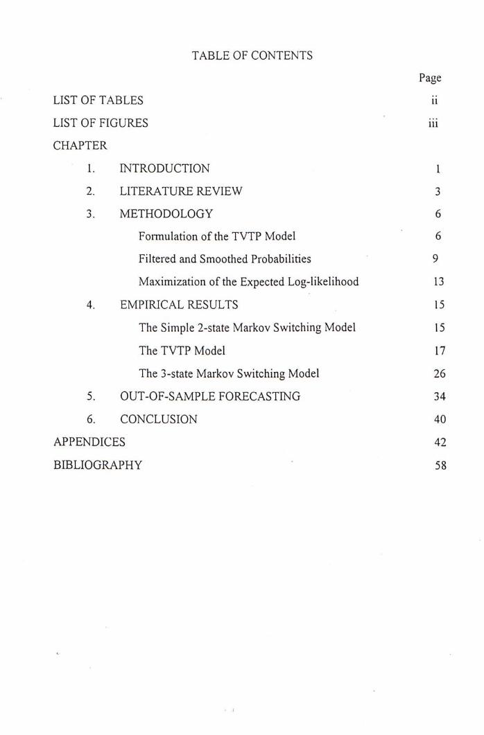
TABLE OF CONTENTS
Page
LIST OF TABLES ii
LIST OF FIGURES iii
CHAPTER
1. INTRODUCTION 1
2. LITERATURE REVIEW 3
3. METHODOLOGY 6
Formulation of the TVTP Model 6
Filtered and Smoothed Probabilities 9
Maximization of the Expected Log-likelihood 13
4. EMPIRICAL RESULTS 15
The Simple 2-state Markov Switching Model 15
The TVTP Model 17
The 3-state Markov Switching Model 26
5. OUT-OF-SAMPLE FORECASTING 34
6. CONCLUSION 40
APPENDICES 42
BIBLIOGRAPHY 58

LIST OF TABLES
Page
Table
1. Parameter Estimates for the 2-state Markov and
the TVTP Model 16
2. Parameter Estimates for the 3-state Markov Model 28
3. Post-sample Root Mean Squared Forecast Errors 36
4. Post-sample Mean Absolute Forecast Errors 37
ii

LIST OF FIGURES
Page
Figure
1. The Smoothed Probabilities of the 2-state Markov and the TVTP Models for Each Currency 18
2. The Transition Probabilities of the TVTP Model for Each Currency 23
3. The Smoothed Probabilities of the 3-state Markov Model for Each Currency 29
iii

CHAPTER 1
INTRODUCTION
Markov-switching model, originally devised by Hamilton, is claimed to
well model a random process which experiences discrete shifts in values of its
underlying parameters. During the past decade, the Markov model is broadly
applied to some economic issues as the business cycles dynamics (Goodwin 1993
and Filardo 1994),the term structure of interest rates (Hamilton 1988), the stock
price volatility (Hamilton and Susmel 1994) and the exchange rate analysis (Engel
and Hamilton 1990; Kaminsky 1993 and Engel 1994). As regard to the topic on
exchange rates, strong evidence has been found that the first difference in the log
of exchange rates of many major currencies experience shifts in regime from low
or negative to high or positive expected values.
Nevertheless, recent literature indicates that only simple 2-state Markov
model or its variant with constant transition probabilities is employed to trace out
the exchange rate movement. Engel (1994) proposed for future development that
the Markov model with more than two states may be operative in the exchange rate
analysis. Filardo (1994) introduced the time-varying instead of constant transition
probabilities (TVTP) in his study of the business cycles dynamics and found a
much better result and forecasting performance. Therefore, a natural question
emerges: can these extensions yield superior exchange rate forecasts when
compared to the simple Markov model, and even the driftless random walk? Or do
these formulations rather weaken the prediction power because oveifitting occurs
or the market fundamentals "distort" the estimates? The argument is based on the
fact that many structural exchange rate models, which use market fundamentals as
explanatory variables, produce unsatisfactory forecasts (Meese and Rogoff 1983).
These questions and corresponding answers constitute the main theme of
the discussion. In this paper, the 3-state Markov and TVTP models are estimated
for the US dollar against the German mark, the Japanese yen and the British pound
exchange rates, and are compared to the simple Markov and random walk models
in terms of forecasting performance. It is believed that these two extensions
should win over the simple 2-state Markov model because they have supportive
underlying rationales. As refer to the 3-state Markov model, Engel (1994) pointed
out that the poorer forecasts offered by the simple 2-state Markov model (when
compared to the zero-drift random walk) can be attributed to the Lourve accord of
March 1987. This accord seems to have stabilized the exchange rates and implied
the occurrence of a new state characterized by low variances and less drift (it is
called narrow spread) during his post-sample forecast period. Therefore, he
argued that the Markov model would perform better if it allowed for a third state
to incorporate the narrow spread characteristics of the exchange rate process. For
the TVTP model, it has extra flexibility to allow the transition probabilities to
adjust before a rise or decline in the exchange rate, and hence helps to identify the
current state or regime and forecast when the exchange rate switches regimes. It is
expected that the structure of the TVTP model is endowed with a satisfactory
prediction power.
The paper is organized as follows. The literature review is presented in
Chapter Two. Chapter Three delineates the formulation of the TVTP model with
the 2-state Markov model as a nested alternative. Chapter Four reports the
estimates of the 2-state and the 3-state Markov, and the TVTP models. Chapter
Five compares their forecasting performance. Conclusions are offered in Chapter
Six.
2
CHAPTER 2
LITERATURE REVIEW
The Markov model was first applied to the exchange rate analysis by Engel
and Hamilton (1990). The motivation of their study was that they observed
apparent long swings in several exchange rates against the dollar over the period
from the third quarter of 1973 to the first quarter of 1988 and this phenomenon
violated predictions from the stiiictural exchange rate models. For instance, if the
US real interest rate was driven up by the fiscal or monetary policies, it would
only result in one-time upward jump in the value of the dollar according to the
Dombusch (1976) sticky price model, and then the dollar would depreciate
gradually to equate the expected return across countries. However, reality told us
the truth that the dollar was instead much stronger for the subsequent one or two
years after a rise in the real interest rate during that period. Therefore, they were
questioned whether the exchange rates were generated by such stochastic process
that incorporated long swings as its systematic part, or just followed a random
walk with the directionless drifts. They applied the Markov model and assumed
any quarter's change in the exchange rate as driving from one of two regimes or
states which corresponded to episodes of a rising or falling rate respectively. The
results were robust in-sample that two different regimes were identified for
corresponding exchange rates and a given regime was likely to persist for several
years to support the phenomenon of long swings. However, the post-sample
forecasting ability of the Markov model was poor when compared to the zero-drift
random walk on the basis of the mean squared forecast error. In order to have a
complete and thorough comparison on the forecasting performance, Engel (1994)
examined eighteen exchange rates and chose thirteen rates as objects for the
contest. The post-sample forecast period began in the second quarter of 1986 and
ended in the first quarter of 1991. It was found that although the Markov model
3

was superior in forecasting the direction of change in exchange rates, it was still
out-performed by the zero-drift random walk in minimizing the mean squared
forecast eiTor.
Kaminsky (1993) argued that the poor forecasting performance of the
Markov irw del could be explained by its implicit assumption that investors used
only past exchange rate observations to make their forecasts. This information set
might not be enough to forecast changes in the economic environment which
would affect the future path of the exchange rate. Therefore, in his framework, it
was assumed that investors also included the announcements made by Federal
Reserve officials in their information set, and the news provided by such
announcements might be wrong in some situations but helped investors to identify
the current exchange rate regime. The model using this "imperfect,’ information
was termed the Markov model with imperfect regime classification information
(IRCI). The monthly dollar per British pound rate over the period from March
1976 to De:ember 1987 was examined, and it was shown that although the IRCI
model h a d � i higher forecasting performance when compared to the simple Markov
model, its forecasts were not superior than those offered by the zero-drift random
walk.
Filardo (1994) proposed another scheme to improve the forecasting
performance of the Markov model in the business cycle analysis. The transition
probabilities of the Markov model were allowed to evolve as a logistic function of
economic indicators, and were called the time varying transition probabilities
(TVTP). Sach flexibility would provide valuable additional information about
whether a particular business cycle phase had occurred and whether a turning
point was imminent. The idea was similar to those of the IRCI model that the
4
indicators helped to identify the current regime (expansion or contraction) which
the economy was in. The US business cycles over the period from January 1948
to August 1992 were considered, and they were measured by the growth rate in the
national output. The logarithmic first difference of seasonally adjusted total
industrial output from Federal Reserve was chosen as a proxy for the growth rate.
Data on the Composite Index of Eleven Leading Indicators, the Stock and Watson
Experimental index of Seven Leading Indicators, the Standard and Poor's
Composite Stock Index and so on were used as the economic indicators. It was
discovered that the TVTP model offered more satisfactory forecasts when
compared to the Markov model and time series models such as the ARJMA and
VAR.
5
CHAPTER 3
METHODOLOGY
The formulation of the TVTP model is presented in this chapter, and the
Markov models can be constructed by following the same rationale. The details of
the Markov models are described in Hamilton (1990,1993 and 1994).
Formulation of the TVTP Model
Following Diebold, Lee and Weinbach (1994), let the regime or state that a
given process is in at time t be indexed by an unobserved random variable s^,
which takes on the value zero or one, and it is assumed that changes in an
exchange rate e, follow such process. When S[ = 0’ the observed change, e is
assumed to be drawn from the N{/uq,ag^ ) distribution, whereas if s^ = 1, e^ is
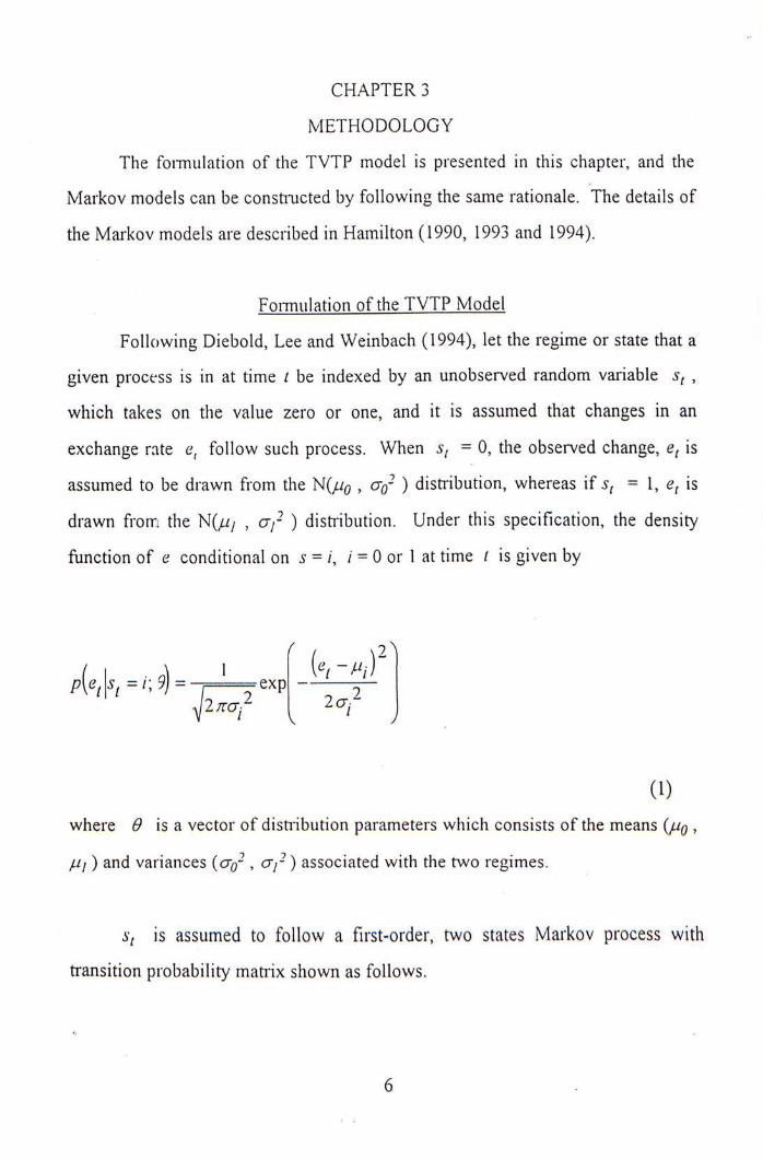
drawn from the N(/// , cr;- ) distribution. Under this specification, the density
function of e conditional on ^ = /.’ i = 0 or I at time I is given by
r W I J
(1)
where <9 is a vector of distribution parameters which consists of the means {juq ,
/u j ) and variances (cr^^ , a;-) associated with the two regimes.
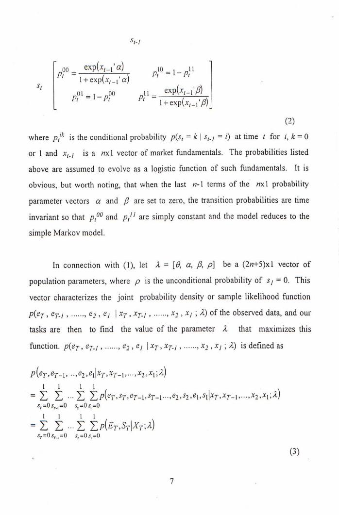
St is assumed to follow a first-order, two states Markov process with
transition probability matrix shown as follows.
i.
6
^'t-l
“ 0 0 - e x p C v i ' … 11 Pt 一 7 — r r Pt — 1 Pt
l + exp(x,_i a )
Pt 二 卜 凡 Pt —i + expOc卜 1,") • J
(2)
where 厂产 is the conditional probability p{Sf = k | s^.j = i) at time t for /•’ 众 = 0
or 1 and is a nxl vector of market fundamentals. The probabilities listed
above are assumed to evolve as a logistic function of such fundamentals. It is
obvious, but worth noting, that when the last n-l terms of the nxl probability
parameter vectors a and P are set to zero, the transition probabilities are time
invariant so that p P � a n d p / i are simply constant and the model reduces to the
simple Markov model.
In connection with (1), let X = [0, a, A p] be a (2«+5)xl vector of
population parameters, where p is the unconditional probability of Sj = 0. This
vector characterizes the joint probability density or sample likelihood function
,(^T-J, , ’ e j I Xt,Xf.j, , X 2 , X j ; X ) of the observed data, and our
tasks are then to find the value of the parameter X that maximizes this
function. p ( c ’ , , I "^r,^T - j,……,, Xj ; X) is defined as
P(叶’ct-I, ..,c)2,q|xr,xr-i,…,巧,义)
= Z Z - Z j : p { E r , S T \ X r a )
(3)
7
and
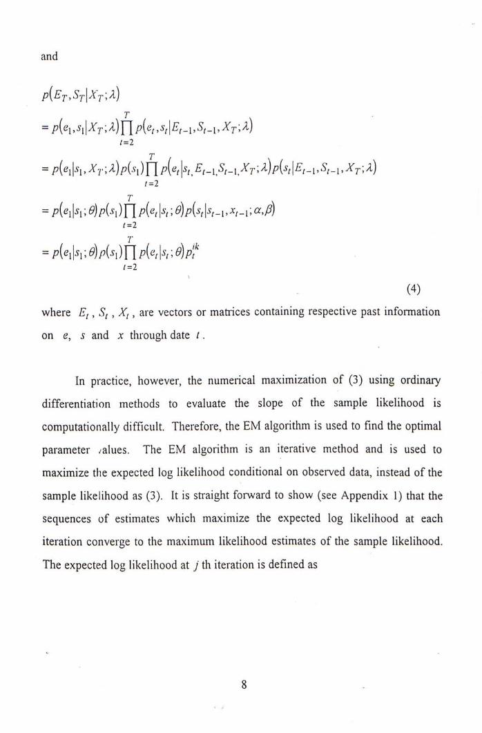
T
= 义 ) f l • , 丑 卜 i,、Vi,而;义)
t=2
T
t=2 T
= h ;约 p(5,i) n pi^t k ; /=2
T
= I 巧;动 p i h ) n pi^t k ;动 pI" t=2
(4)
where E^,S^,Xi,are vectors or matrices containing respective past information
on e, s and x through date i .
In practice, however, the numerical maximization of (3) using ordinary
differentiation methods to evaluate the slope of the sample likelihood is
computationally difficult. Therefore, the EM algorithm is used to find the optimal
parameter .'alues. The EM algorithm is an iterative method and is used to
maximize the expected log likelihood conditional on observed data, instead of the
sample likelihood as (3). It is straight forward to show (see Appendix 1) that the
sequences of estimates which maximize the expected log likelihood at each
iteration converge to the maximum likelihood estimates of the sample likelihood.
The expected log likelihood at j th iteration is defined as
8
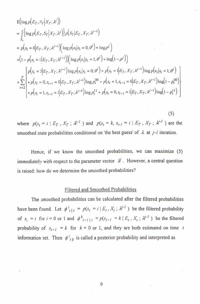
= [ \ o g p [ E r , S - f Xf
Sr
= = o | £ 7 , ’ A V ; A 厂 i)(logp(c’|«Sl =0;…+log/y.夕
+ ( 1 - • 二 拉 , ’ A V ; 1 ) ) [ " l o g • |、.i 二 1 ; … + 1 o g ( 1 V )
• \ 7
丁
⑶
where 厂 = i \ Ej , Xj ; ) and = k, s^., = i \ E-p , X^ • ) are the
smoothed state probabilities conditional on 丨 the best guess' of A at j-l iteration.
Hence, if we know the smoothed probabilities, we can maximize (5)
immediately with respect to the parameter vector M . However, a central question
is raised: how do we determine the smoothed probabilities?
Filtered and Smoothed Probabilities
The smoothed probabilities can be calculated after the filtered probabilities I
have been found. Let zW, | , = p{st = \ ?J'' ) be the filtered probability
of St = i for i = 0 or I and 於人 )十 / 1 , = 广 = k \ E" X^ 刃‘丨、be the filtered
probability of s^+j = k for k = Q or 1,and they are both estimated on time t
information set. Then ( j ) � i s called a posterior probability and interpreted as
9
/ \
, M c ' M • 广 - 1 , 义 " 义 广 \ = ] — ,
/ \ / \
_ 巧二。伊-1)厂(‘s) =/|E,-i,义/-i;义广\
/ \
一 M � k / •;没,-1)4-1
— • I五丨,义H ;义广 i )
(6)
where
(7)
and (j>^t+i\ t is called a prior probability and interpreted as
1 /=0
(8) j
where 丨力=/; ) is given by (1).
It is more convenient to express the derivation of the filtered probabilities in
matrix form. Let O , = [(f) \\t ’ ^t\t ]’ ^t+i\t =、伞 V / ] / ’ <t> ] and n广=
[p{e^ I 5广 0 ; 0 J - 1 � , I = 1 ; … " ) ] b e the matrices considered here. Then
10 .
(9)
and
�;+i | /=P/, i � ; k
(10)
Where P/+/ is the transition probability matrix as (2),and 1 is a column vector
whose elements are unity. The symbol * denotes element-by-element
multiplication.
Using (9) and (10), one can calculate the values of filtered probabilities �,丨,
and for each time t by iteration in the sample. Given the filtered
probabilities, the smoothed probabilities can be determined by following the
algorithm developed by Kim (1993). Let • = Pih = i \ Ej , Xj \ be the
smoothed probability of s^ = i on the time T information set and defined as
11
k=0
= Z / 4 + 1 二 众 |/ r,义 7,乂 二 小7+1 ="’五,’义。义叫 A: 二 0
f .-iV
= I : M-s’,+i = "五 r ,义 r ;义广 , .
/ \ ^
= 1 : / i ? , 卞 | 二 " | 五 r ’ 义 r ; 义 广 — — — — T ^
/ \
. 丨 、 乂 二 • + � , r ’ 义 r ; 广 1)
=p[S( = i ^ k=o = 五 / , 知 广 j
- / 4 + i = 0| 知 , 义 r;义广 1)
= • 卡 , ; 义 p i l l ]
(11)
provided that 厂 ( 〜 = i | V y 二 k , Et ’ 乂丁., ^!'') = = i | s …=k^E^.X^-, ?J'^) •
The algorithm can be made clear and compact in matrix form as
�The details of the proof can be found in Hamilton (1994).
12 .
(12)
where ^ ]• The symbol (+) denotes element-by-element division.
Therefore, the smoothed probabilities can be found by iterating on (12) backward
for t = T-1, T-2, 2, I. It is worth noting that the algorithm starts with Oj^j^
which is obtained from (9) for t = T.
Maximization of the Expected Log-likelihood
After the smoothed probabilities are obtained, the expected log likelihood
(5) is maximized directly with respect to the parameter M. The resulting 2n+5
expressions for the likelihood estimates are listed as follows.
T _
J - l^i h 一 丁 . I、
(13)
T 2 / .一 1、
YM -Mi) M � = z | £ v,A > ;乂广
rP- - i ^ 《一 T .,、
(14)
for / = 0, 1
(15)
13 .
r { 「 ; ; I 00 1 �
^ >卜 | 厂 “ =0’‘y卜 1 二 0|£',,A V ;义广•卜 1 广 1) p ? ' - — / L Jz
“ 一丁
(16)
T { / , \ . , \ ,, dp^ 1 .,
n - — — - ^
T (
r=2 P
(17)
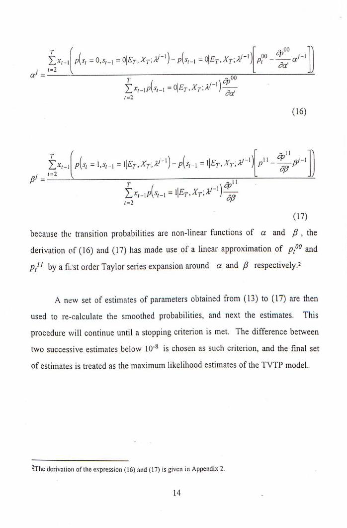
because the transition probabilities are non-linear functions of a and /? , the
derivation of (16) and (17) has made use of a linear approximation of 严 and
p/i by a fi:-st order Taylor series expansion around a and (5 respectively.2
A new set of estimates of parameters obtained from (13) to (17) are then
used to re-calculate the smoothed probabilities, and next the estimates. This
procedure will continue until a stopping criterion is met. The difference between
two successive estimates below 10"^ is chosen as such criterion, and the final set
of estimates is treated as the maximum likelihood estimates of the TVTP model.
2;rhe derivation of the expression (16) and (17) is given in Appendix 2.
14 ,
CHAPTER 4
EMPIRICAL RESULTS
The exchange rates examined in this paper are the US dollar against the
German mark, the Japanese yen and the British pound. Monetary theories state
that the exchange rate could be affected by such exogenous variables as the
difference in money supply changes, the difference in output changes, the
difference in interest rates and the difference in inflation rates between the
corresponding countries. Therefore, various combinations of the lagged values of
these variables have been attempted as the market fundamentals to influence the
transition probabilities, and it is observed that the interest rate differential ( R^, ,)
as proxied by the treasury bill rate differential or the call money rate differential
alone does the best in estimation and forecasting and its results are reported in this
thesis (the results produced by other combinations are also tried). In mathematical
term, this functional relation can be expressed as p!�=/( x^.j ) = / ( R^.j ) • The
data on exchange rates and market fundamentals are monthly series and obtained
from the International Financial Statistics (IFS). The sample period begins in
January 1976 for German mark and in September 1973 for Japanese yen and
British pound, and ends in January 1988. The starting point of the sample period
for each currency depends on the availability of data.
The Simple 2-state Markov Switching Model
The results are summarized in Table 1, and it can be seen that some
estimates on means are significant at the 5 or 10 percent level.^
^The estimates on the un-conditional probability p for each model are suppressed from Tables I and 2 because they are not the main concern of this paper.
15 .
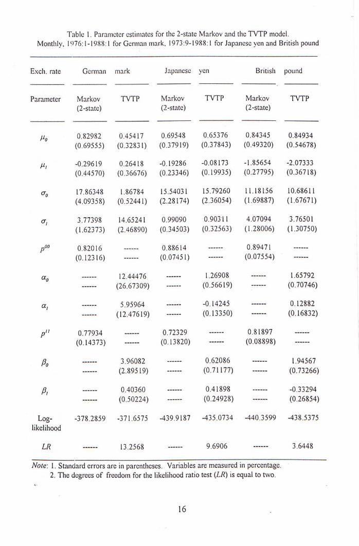
Table I. Parameter estimates for the 2-state Markov and the T V T P model. Monthly , 1976:1-1988:1 for German mark, 1973:9-1988:1 for Japanese yen and British pound
Exch. rate German mark Japanese yen British pound
Parameter Markov T V T P Markov T V T P Markov T V T P (2-state) (2-state) (2-state)
jjo 0 . 8 2 9 8 2 0 . 4 5 4 1 7 0 . 6 9 5 4 8 0 . 6 5 3 7 6 0 . 8 4 3 4 5 0 . 8 4 9 3 4
( 0 . 6 9 5 5 5 ) ( 0 . 3 2 8 3 1 ) ( 0 . 3 7 9 1 9 ) ( 0 . 3 7 8 4 3 ) ( 0 . 4 9 3 2 0 ) ( 0 . 5 4 6 7 8 )
… - 0 . 2 9 6 1 9 0 . 2 6 4 1 8 - 0 . 1 9 2 8 6 - 0 . 0 8 1 7 3 - 1 . 8 5 6 5 4 - 2 . 0 7 3 3 3
( 0 . 4 4 5 7 0 ) ( 0 . 3 6 6 7 6 ) ( 0 . 2 3 3 4 6 ) ( 0 . 1 9 9 3 5 ) ( 0 . 2 7 7 9 5 ) ( 0 . 3 6 7 1 8 )
(jo 1 7 . 8 6 3 4 8 1 .86784 15 .54031 1 5 . 7 9 2 6 0 1 1 . 1 8 1 5 6 1 0 . 6 8 6 1 1
( 4 . 0 9 3 5 8 ) ( 0 . 5 2 4 4 1 ) ( 2 . 2 8 1 7 4 ) ( 2 . 3 6 0 5 4 ) ( 1 . 6 9 8 8 7 ) ( 1 . 6 7 6 7 1 )
o ) 3 . 7 7 3 9 8 14 .65241 0 . 9 9 0 9 0 0 . 9 0 3 1 1 4 . 0 7 0 9 4 3 . 7 6 5 0 1
( 1 . 6 2 3 7 3 ) ( 2 . 4 6 8 9 0 ) ( 0 . 3 4 5 0 3 ) ( 0 . 3 2 5 6 3 ) ( 1 . 2 8 0 0 6 ) ( 1 . 3 0 7 5 0 )
p。o 0.82016 …… 0.88614 —— 0.89471 ——
(0.12316) - ( 0 . 0 7 4 5 1 ) -…-- (0.07554) -…―
… … 12.44476 -…“ 1.26908 ------ 1.65792
-…-- (26.67309) -…― (0.56619) -…-- (0.70746)
cCi —— 5 . 9 5 9 6 4 0 . 1 4 2 4 5 —— 0 . 1 2 8 8 2
‘ -…― (12.47619) -…-- (0.13350) -…-- (0.16832)
p" 0 . 7 7 9 3 4 —— 0 . 7 2 3 2 9 —— 0 . 8 1 8 9 7 ——
(0.14373) -…— (0.13820) -“… (0.08898) -…—
Po —— 3 . 9 6 0 8 2 —— 0 . 6 2 0 8 6 —— 1 . 9 4 5 6 7 —— (2 .89519) —— ( 0 . 7 U 7 7 ) —— (0 . 7 3 2 6 6 )
—— 0 . 4 0 3 6 0 —— 0 . 4 1 8 9 8 0 . 3 3 2 9 4 -…― (0.50224) -…-- (0.24928) -…-- (0.26854)
L o g - - 3 7 8 . 2 8 5 9 - 3 7 1 . 6 5 7 5 - 4 3 9 . 9 1 8 7 - 4 3 5 . 0 7 3 4 - 4 4 0 . 3 5 9 9 - 4 3 8 . 5 3 7 5
l ikelihood
LR —— 13 .2568 —— 9 . 6 9 0 6 —— 3 . 6 4 4 8
Note: 1. Standard errors are in parentheses. Variables are measured in percentage.
2. T h e degrees o f freedom for the l ikelihood ratio test {LR) is equal to two.
16 .
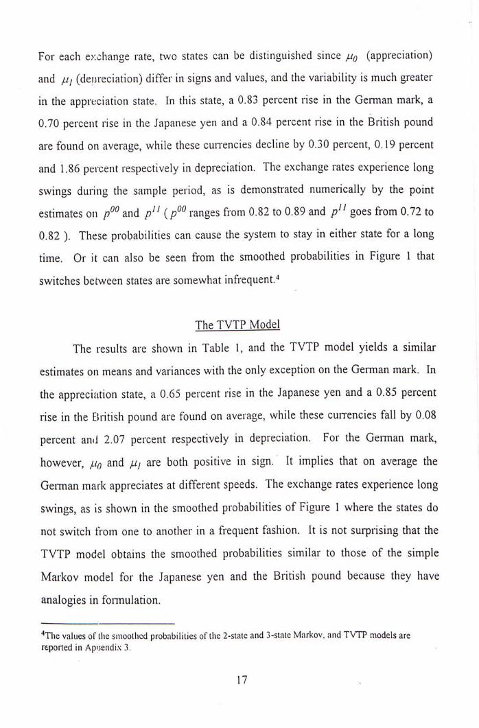
For each exchange rate, two states can be distinguished since juq (appreciation)
and jjj (denreciation) differ in signs and values, and the variability is much greater
in the appreciation state. In this state, a 0.83 percent rise in the German mark, a
0.70 percent rise in the Japanese yen and a 0.84 percent rise in the British pound
are found on average, while these currencies decline by 0.30 percent, 0.19 percent
and 1.86 percent respectively in depreciation. The exchange rates experience long
swings during the sample period, as is demonstrated numerically by the point
estimates on 卯 and p " (p卯 ranges from 0.82 to 0.89 and p " goes from 0.72 to
0.82 ). These probabilities can cause the system to stay in either state for a long
time. Or it can also be seen from the smoothed probabilities in Figure 1 that
switches between states are somewhat infrequent."^
The TVTP Model
The results are shown in Table 1,and the TVTP model yields a similar
estimates on means and variances with the only exception on the German mark. In
the appreciation state, a 0.65 percent rise in the Japanese yen and a 0.85 percent
rise in the British pound are found on average, while these currencies fall by 0.08
percent and 2.07 percent respectively in depreciation. For the German mark,
however, /.Iq and juj are both positive in sign. It implies that on average the
German mark appreciates at different speeds. The exchange rates experience long
swings, as is shown in the smoothed probabilities of Figure 1 where the states do
not switch from one to another in a frequent fashion. It is not surprising that the
TVTP model obtains the smoothed probabilities similar to those of the simple
Markov model for the Japanese yen and the British pound because they have
analogies in formulation.
� T h e values of the smoothed probabilities of the 2-statc and 3-state Markov, and TVTP models are reported in Apoendix 3.
17 .
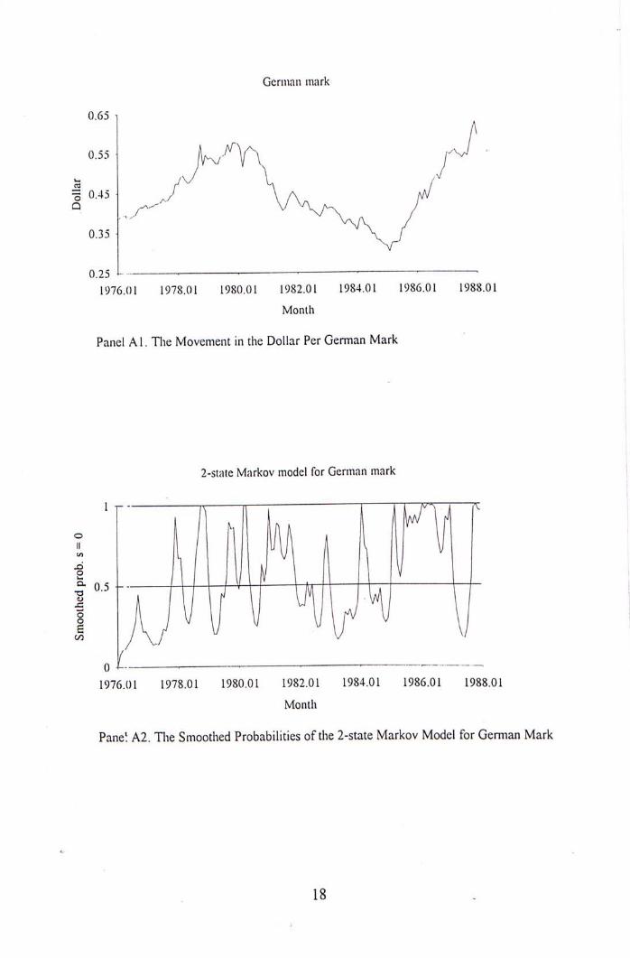
German mark
0.65
0.25 I" ‘ 1976.01 1978.01 1980.01 1982.01 1984.01 1986.01 1988.01
Month
Panel A1 • The Movement in the Dollar Per German Mark
2-state Markov model for German mark ' [ I I ji rjFjr I I m I V I . V _ L r ^ j W W H f
f 0 ‘ ‘ ‘ “ ‘
1976.01 1978.01 1980.01 1982.01 1984.01 1986.01 1988.01
Month
Pane: A2. The Smoothed Probabilities o f the 2-state Markov Model for German Mark
18 .
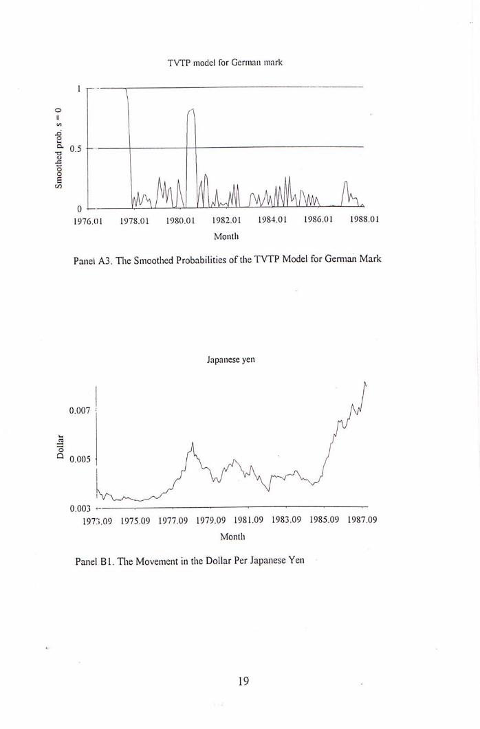
TVTP model for German mark
I r “ “
T n • t/i
^ 0.5 (U O O K
‘ J I m M I f i l i J I、aAI\ma • k
1976.01 1978.01 1980.01 1982.01 1984.01 1986.01 1988.01 Month
Panel A3. The Smoothed Probabilities of the T V T P Model for German Mark
Japanese yen
I / 0.007 • / V
。 。 “ . A / X r ^ y 0.003 — , ‘
197:;.09 1975.09 1977.09 1979.09 1981.09 1983.09 1985.09 1987.09
Month
Panel B l . The Movement in the Dollar Per Japanese Yen
19 ,
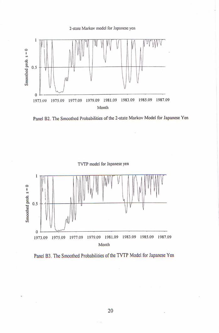
2-state Markov model for Japanese yen
。 I f f ! i _ i 哪 1/1 i i r t f 擎
1 I “ 『 I .
1 I V V F 0 —^^‘ ‘
1973.09 1975.09 1977.09 1979.09 1981.09 1983.09 1985.09 1987.09
Month
Panel B2. The Smoothed Probabilities of the 2-state Markov Model for Japanese Yen
TVTP model for Japanese yen !
i ' l Q E W : I 0.5 - t f I P | H | 1
I IM f : o L _ _ ^ .
1973.09 1975.09 1977.09 1979.09 1981.09 1983.09 1985.09 1987.09 Month
Panel B3. The Smoothed Probabilities of the TVTP Model for Japanese Yen
20 .
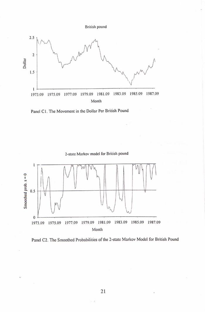
British pound
T 〜 y \ .
c、,\\ \
I ‘ 1973.09 1975.09 1977.09 1979.09 1981.09 1983.09 1985.09 1987.09
Month
Panel C I . The Movement in the Dollar Per British Pound
2-state Markov model for British pound
【 n A A r ^ i N v r M n / | I A V h I / w 』/ [fj u
0 ‘ — 1973.09 1975.09 1977.09 1979.09 1981.09 1983.09 1985.09 1987.09
Month Panel C2. The Smoothed Probabilities of the 2-state Markov Model for British Pound
21 ,
TVTP model for British pound
1 p w i M n n 1 1 fflfvi
J l\lUW ^ \ V • 1 0 . 5 - j - i t H \ r r i M l — ^
1 i \r lUl 0 J ‘
1973.09 1975.09 1977.09 1979.09 1981.09 1983.09 1985.09 1987.09 Month
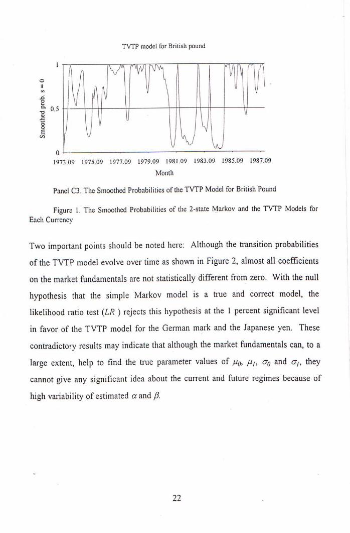
Panel C3. The Smoothed Probabilities of the T V T P Model for British Pound Figure I. The Smoothed Probabilities o f the 2-state Markov and the T V T P Models for
Each Currency
Two important points should be noted here: Although the transition probabilities |
of the TVTP model evolve over time as shown in Figure 2, almost all coefficients
on the market fundamentals are not statistically different from zero. With the null i
hypothesis that the simple Markov model is a true and correct model, the
likelihood ratio test (LR ) rejects this hypothesis at the 1 percent significant level
in favor of the TVTP model for the German mark and the Japanese yen. These
contradictory results may indicate that although the market fundamentals can, to a
large extern, help to find the true parameter values of /Uq, "/,cr^ and cr卜 they
cannot give any significant idea about the current and future regimes because of
high variability of estimated a and p.
22 ,
TVTP model for German mark
。 ' n r n n r i 0.5 1 " H H I I 1
o L u J J ~ 1 1 1 1 。 ~ l U Z _ _ U 1976.01 1978.01 1980.01 1982.01 1984.01 1986.01 1988.01
Month
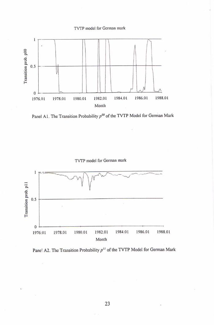
Panel A l . The Transition Probability o f the T V T P Model for German Mark
TVTP model for German mark
— 1 「 〜 、 ^ Y " ^ 八 〜 〜 〜
X) 2 CU c 0.5
.2
c 2 H
0 -L————‘ ‘ ‘ ^ 1976.01 1978.01 1980.01 1982.01 1984.01 1986.01 1988.01
Month
Pane!八2. The Transition Probability p" o f the T V T P Model for German Mark
I.
23 -
TVTP model for Japanese yen
。 ‘ [ 广 〜 一 • . 、 , — _
1 V 〜 " ^ • a 0.5 o •Z75 c 2 H
0 ‘ 1973.09 1975.09 1977.09 1979.09 1981.09 1983.09 1985.09 1987.09
Month
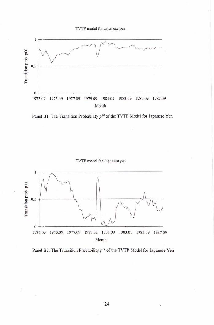
Panel B l . The Transition Probability p � � o f the T V T P Model for Japanese Yen
i i
TVTP model for Japanese yen I
! ) 广 - \ n
u —~‘ ‘ ‘ ‘ ‘ — ^ 1973.09 1975.09 1977.09 1979.09 1981.09 1983.09 1985.09 1987.09
Month
Pane) B2. The Transition Probability p" o f the T V T P Model for Japanese Yen
I.
24 .
TVTP model for British pound
1 1
g 八 一 、 一 — - 、
u.
a 0.5 0 G 03 H
0 ‘ — — 1973.09 1975.09 1977.09 1979.09 1981.09 1983.09 1985.09 1987.09
Month
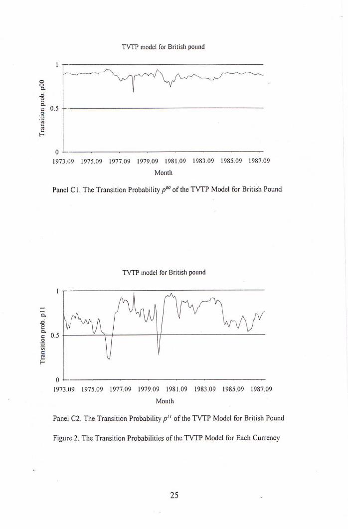
Panel C I . The Transition Probability / � o f the T V T P Model for British Pound
TVTP model for British pound
1 l i V H
0 J ‘ ‘ 1973.09 1975.09 1977.09 1979.09 1981.09 1983.09 1985.09 1987.09
Month
Panel C2. The Transition Probability p" o f the T V T P Model for British Pound
Figur-j 2. The Transition Probabilities o f the T V T P Model for Each Currency
25 .

The 3-state Markov Switching Model
The results are shown in Table 2, and it should be noted that in estimating
the 3-state Markov model, some are constrained to zero or one because their
unrestricted maximum likelihood estimates fall on the boiindaiy and this would
violate the regularity conditions to calculate the inverse of the information matrix
and hence the asymptotic standard errors. It can be seen that some estimates on
means are significant at the 5 or 10 percent l e v e l . ^ The appreciation, the
depreciation and the narrow spread states can be distinguished for each exchange
rate since / / … a n d differ in signs or values. The variability is higher in the
depreciation state for the German mark and the Japanese yen, while in the
appreciation state for the British pound. A 0.42 percent decline in the German
mark, a 0.03 percent rise in the Japanese yen and a 0.72 percent rise in the British
pound are found on average in the narrow spread state. These currencies rise by
5.25 percent, 5.20 percent and 2.01 percent in appreciation while decline in value
by 1.79 percent, 1.93 percent and 1.60 percent in depreciation respectively. Some
interesting features are observed: [1] when the German mark is in the depreciation
state, it will switch to the appreciation state next period (given p冗 is one), [2'
when the British pound is in the narrow spread state, it will never move to the
appreciation state next period (given p^^ is zero), [3] when the British pound is in
the depreciation state, it will never switch to the narrow spread state next period
(given is zero), [4] the German mark stays at the narrow spread state in a
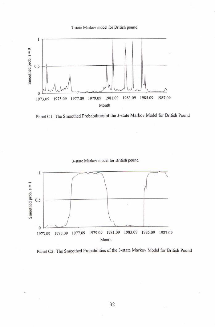
frequent fashion, as is shown in the smoothed probabilities of Figure 3,and [5] the
Japanese yen and the British pound experience long swings during the sample
^For 3-state Markov model, the transition probability matrix is defined as
- 尸 0 0 ^ 1 0 尸 2 0 -
P = . 1 - / / ^ 0 _ , , 0 1
26 ,

period, as is justified by the point estimates of p" and p— ( p " ranges from 0.77
to 0.98 and p - goes from 0.71 to 0.88 ),or by the smoothed probabilities in Figure
o J .
27 .
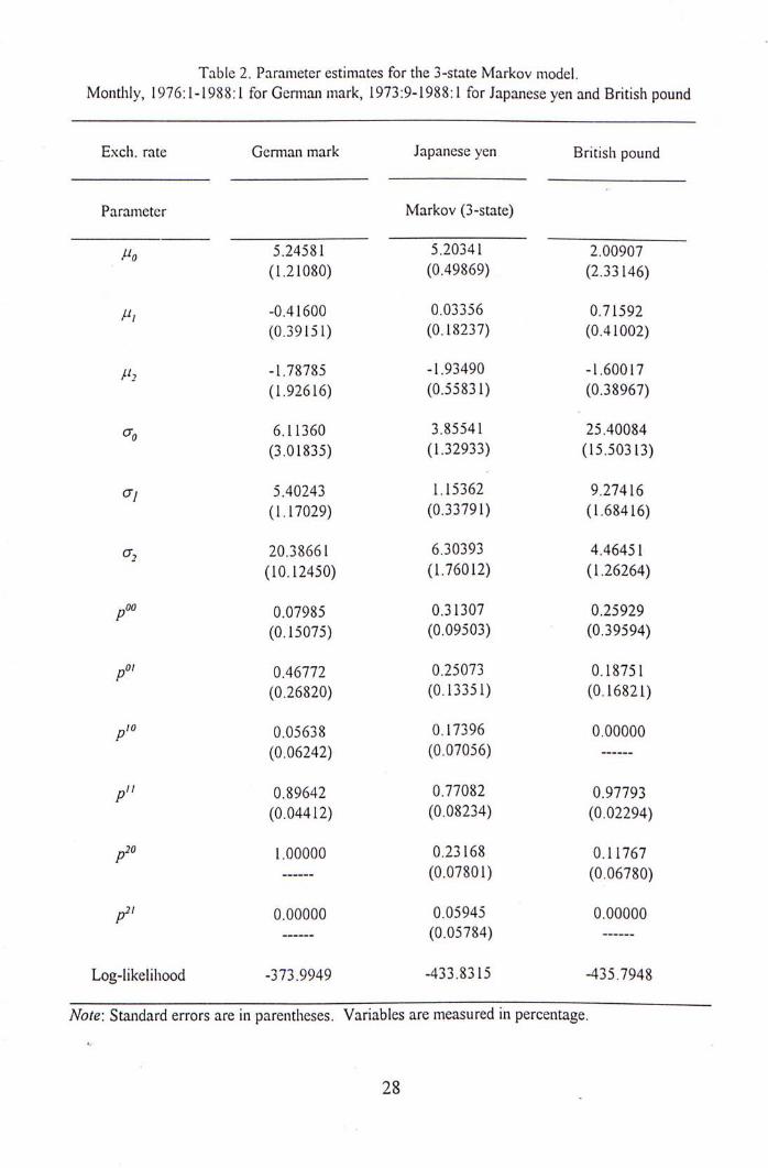
Table 2. Parameter estimates for the 3-state Markov model.
Monthly , 1976:1 -1988:1 for German mark,1973:9-1988:1 for Japanese yen and British pound
Exch. rate German mark Japanese yen British pound
Parameter Markov (3-state)
^ 5 . 2 4 5 8 1 5 . 2 0 3 4 1 2 . 0 0 9 0 7
( 1 . 2 1 0 8 0 ) ( 0 . 4 9 8 6 9 ) ( 2 . 3 3 1 4 6 )
/Ui - 0 . 4 1 6 0 0 0 . 0 3 3 5 6 0 . 7 1 5 9 2
( 0 . 3 9 1 5 1 ) ( 0 . 1 8 2 3 7 ) ( 0 . 4 1 0 0 2 )
- 1 . 7 8 7 8 5 - 1 . 9 3 4 9 0 - 1 . 6 0 0 1 7
‘ ( 1 . 9 2 6 1 6 ) ( 0 . 5 5 8 3 1 ) ( 0 . 3 8 9 6 7 )
cTq 6 . 1 1 3 6 0 3 . 8 5 5 4 1 2 5 . 4 0 0 8 4
( 3 . 0 1 8 3 5 ) ( 1 . 3 2 9 3 3 ) ( 1 5 . 5 0 3 1 3 )
cry 5 . 4 0 2 4 3 1 . 1 5 3 6 2 9 . 2 7 4 1 6
( 1 . 1 7 0 2 9 ) ( 0 . 3 3 7 9 1 ) ( 1 . 6 8 4 1 6 )
cr, 2 0 . 3 8 6 6 1 6 . 3 0 3 9 3 4 . 4 6 4 5 1
“ ( 1 0 . 1 2 4 5 0 ) ( 1 . 7 6 0 1 2 ) ( 1 . 2 6 2 6 4 )
pOo 0 . 0 7 9 8 5 0 . 3 1 3 0 7 0 . 2 5 9 2 9
( 0 . 1 5 0 7 5 ) ( 0 . 0 9 5 0 3 ) ( 0 . 3 9 5 9 4 )
p0' 0 . 4 6 7 7 2 0 . 2 5 0 7 3 0 . 1 8 7 5 1
( 0 . 2 6 8 2 0 ) ( 0 . 1 3 3 5 1 ) ( 0 . 1 6 8 2 1 )
p'o 0 . 0 5 6 3 8 0 . 1 7 3 9 6 0 . 0 0 0 0 0
( 0 . 0 6 2 4 2 ) ( 0 . 0 7 0 5 6 ) -…—
p" 0 . 8 9 6 4 2 0 . 7 7 0 8 2 0 . 9 7 7 9 3
( 0 . 0 4 4 1 2 ) ( 0 . 0 8 2 3 4 ) ( 0 . 0 2 2 9 4 )
广 1.00000 0.23168 0.11767
—— (0.07801) (0.06780)
p2 丨 0 . 0 0 0 0 0 0 . 0 5 9 4 5 0 . 0 0 0 0 0 —— (0.05784) ——
Log- l ike l ihood - 3 7 3 . 9 9 4 9 - 4 3 3 . 8 3 1 5 - 4 3 5 . 7 9 4 8
Note: Standard errors are in parentheses. Variables are measured in percentage.
28
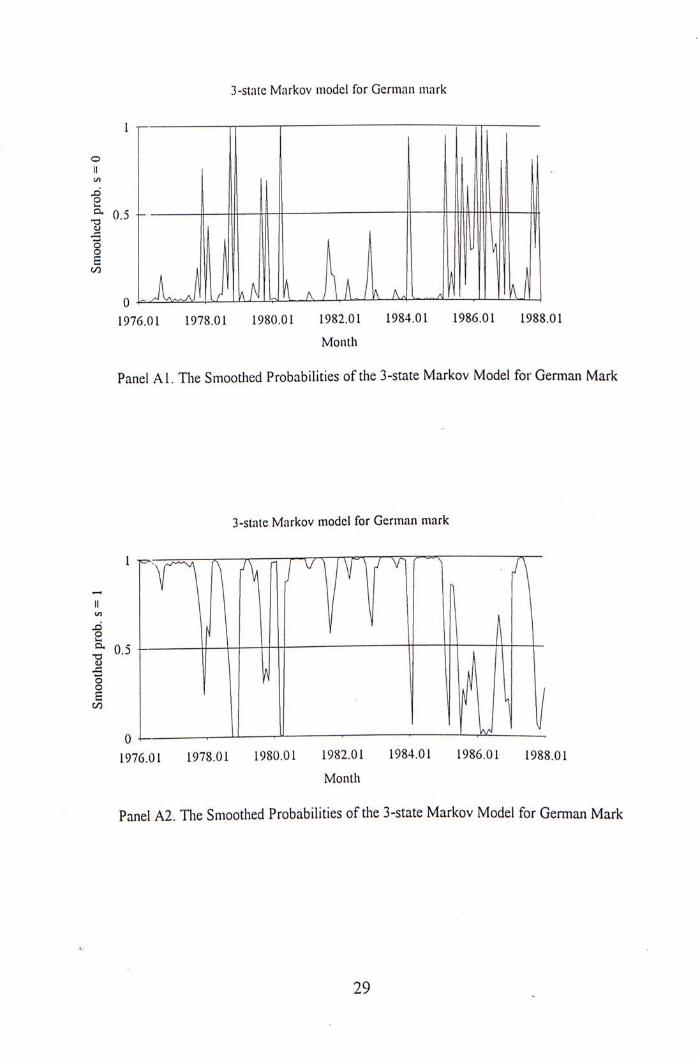
3-state Markov model for German mark
I 1 n
I.-4I1——[Mi I i i i i i n i n 。l i J i J i u i A AIu / I ajI j f i II l y
1976.01 1978.01 1980.01 1982.01 1984.(U 1986.01 1988.01
Month
Panel A l . The Smoothed Probabilities o f the 3-state Markov Model for German Mark
3 - s t a t e Markov model for German mark
I) 『\i 1 1 J\ I I M 」 _ _ J L 1 0.5 f t i — I t f t t I ^ J I S .
� 1 o i ^ J L i ^ — — -
1976.01 1978.01 1980.01 1982.01 1984.01 1986.01 1988.01 Month
Panel A2 . The Smoothed Probabilities o f the 3-state Markov Model for German Mark
29 ,
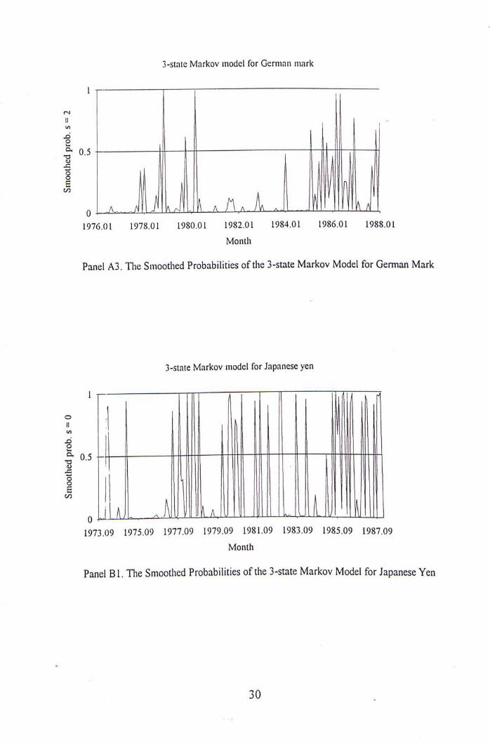
3-state Markov model for German mark
, ' f ^ n p .
卜 l i l h r r t t l J . J i l t J Ik . n A A . I f i n i U I
1976.01 1978.01 1980.01 1982.01 1984.01 1986.01 1988.01 Month
Panel A3. The Smoothed Probabilities o f the 3-state Markov Model for German Mark
3-state Markov model for Japanese yen
! I [ T i l I I I I I I I 1 - ! " 一 h i i r r H 0 1 C/3 I
。丨 i “ j i J i l l 1111 lift A m i l l III 丨 II i L n i m . 11) I 111 III 1973.09 1975.09 1977.09 1979.09 1981.09 1983.09 1985.09 1987.09
Month Panel B l . The Smoothed Probabilities o f the 3-state Markov Model for Japanese Yen
30 .
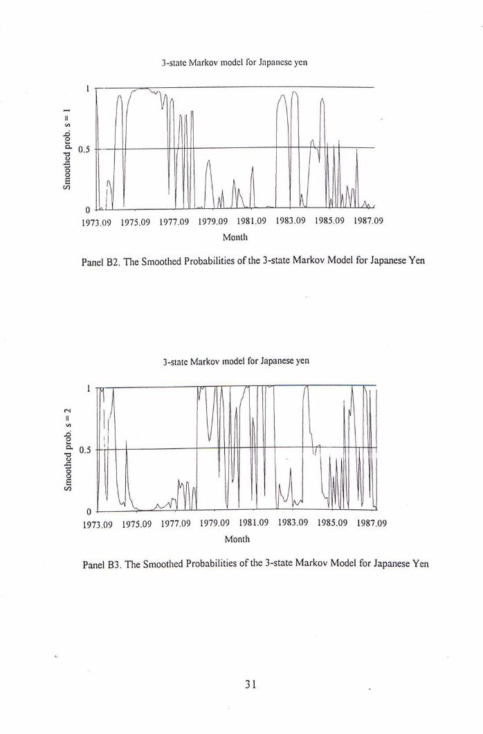
3-slate Markov model for Japanese yen
一 A / ^ A H a II f| (1 . ( / )
X)
1 0 . 5 … 4 | m\ —
‘ J i l IllUfrJ III I I IL 1973.09 1975.09 1977.09 1979.09 1981.09 1983.09 1985.09 1987.09
Month
Panel B2. The Smoothed Probabilities of the 3-state Markov Model for Japanese Yen
3-slate Markov model for Japanese yen
i f T n i i i i / i i i n 11”TT 7 ) L i L V i . 1 I 0.5 H | - 1 - . 1/1 I | |
‘ j . i l l J l i I I Iw i l l 1973.09 1975.09 1977.09 1979.09 1981.09 1983.09 1985.09 1987.09
Month Panel B3. The Smoothed Probabilities o f the 3-state Markov Model for Japanese Yen
31 .
3-state Markov model for British pound
I 1 —
o II .. 1/5
} ^^ 1
1973.09 1975.09 1977.09 1979.09 1981.09 1983.09 1985.09 1987.09
Month
Panel C I . The Smoothed Probabilities o f the 3-state Markov Model for British Pound
3-state Markov model for British pound
1 ,飞 厂 、
JD 2 ; 0 . 5 <U
‘ J I 0 “—— —^ ^ ^ ^
1973.09 1975.09 1977.09 1979.09 1981.09 1983.09 1985.09 1987.09 Month
Panel C2. The Smoothed Probabilities o f the 3-state Markov Model for British Pound
32 ,
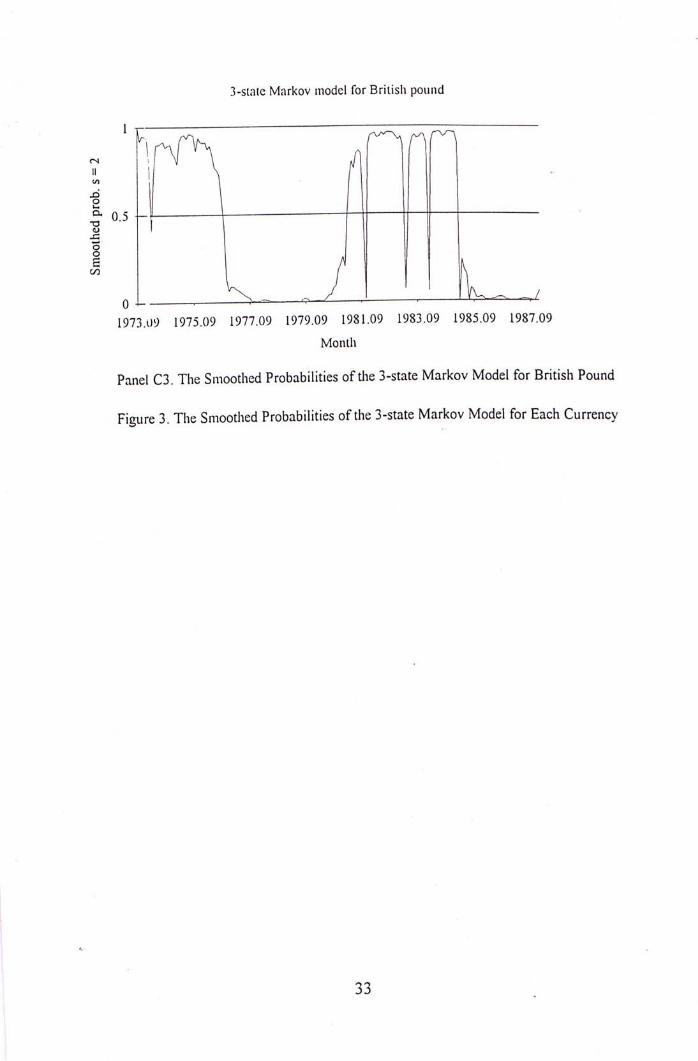
3-state Markov model for British pound
I n fiRnn ^ 0 5
1 丨 n n n
1973.09 1975.09 1977.09 1979.09 1981.09 1983.09 1985.09 1987.09
Month
Panel C3. The Smoothed Probabilities o f the 3-state Markov Model for British Pound
Figure 3. The Smoothed Probabilities o f the 3-state Markov Model for Each Currency
33 .
CHAPTER 5
OUT-OF-SAMPLE FORECASTING
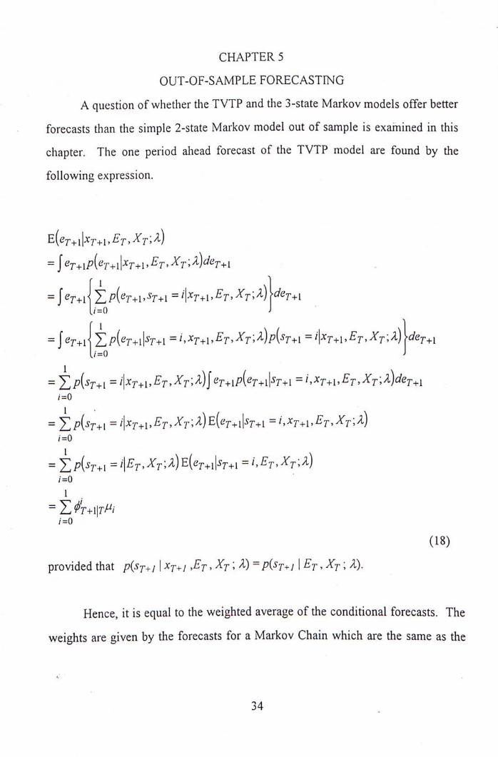
A question of whether the TVTP and the 3-state Markov models offer better
forecasts than the simple 2-state Markov model out of sample is examined in this
chapter. The one period ahead forecast of the TVTP model are found by the
following expression.
E ( c y + i | � + I , & 义 r;义)
= J " c Y + i P ( c Y + i k r + i ’ 五r,义r;义)"cY+i
l/=o
l/=o ‘
= H 行 + 1 , 五 ' 厂 , 和 ; 义 ) J 印 二 五 r , 和 ; 义 印 + 1 /=0
= = 和 r+i,"^r,义 r ; 义 ) = ,,"^7>1,丑 r ’ 义 r;义)
/=0
= S P ( 叶 + 1 = Et,XT.’X)E(cy+1 I T +i 二 /•,知,;义)
/=o 1
i=0
(18)
provided that 厂(叶+/1 � + / ’五r,义r ; 义 ) 丨 五 r , 义 r ;义).
Hence, it is equal to the weighted average of the conditional forecasts. The
weights are given by the forecasts for a Markov Chain which are the same as the
34 ,

filtered probabilities, (jj了+ 丨\丁 . These probabilities are determined by (8) or (10).
The m-period ahead forecast can be made by following the same rationale.
The forecasting period goes from February 1988 to June 1992. The choice
of when to start forecasting is arbitrary. The rolling regression technique is
applied to l e-estimate the parameters of three models for each forecast period in
order to fully utilize the most up-to-date information. Forecasts are generated at
the one, thi se, six, twelve and twenty-four month horizons and in the ex-post sense
for the TVTP model. It is assumed that the future values of the market
fundamentals are known with certainty. Minimization of the root mean squared
error (RMSE) and the mean absolute error (MAE) are chosen as measures to judge
the out-of-sample accuracy. The RMSE and the MAE are shown in Tables 3 and
4, and first consider the comparison between the 2-state and the 3-state Markov
model. The 3-state Markov model has the lower RMSE at the six, twelve and
twenty-four-month horizons for the German mark, at the one, six, twelve and
twenty-four-month horizons for the Japanese yen, and at the six and twenty-four-
month horizons for the British pound. Based on the MAE criterion, it out-
peifoiTns the 2-state Markov model at the six and twelve-month horizons for the
German mark, at all horizons for the Japanese yen, and at the twenty-four month
horizon for the British pound. These results indicate that the 3-state Markov
model performs much better for the Japanese yen. They are consistent with the
higher in-sample log-likelihood value in contrast with the simple 2-state Markov
model as shown in Table 2.
35 .
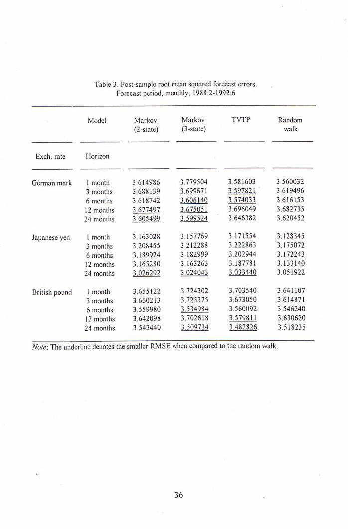
Table 3. Post - sample root mean squared forecast errors. . Forecast period, monthly, 1 9 8 8 : 2 - 1 9 9 2 : 6
Model Markov Markov T V T P Random (2-state) (3-state) walk
Exch. rate Horizon
German mark 1 month 3 . 6 1 4 9 8 6 3 . 7 7 9 5 0 4 3 . 5 8 1 6 0 3 3 . 5 6 0 0 3 2 3 months 3 . 6 8 8 1 3 9 3 . 6 9 9 6 7 1 3 . 5 9 7 8 2 1 3 . 6 1 9 4 9 6
6 months 3 . 6 1 8 7 4 2 3 . 6 0 6 1 4 0 3 . 5 7 4 0 3 3 3 . 6 1 6 1 5 3
12 months 3 . 6 7 7 4 9 7 3 . 6 7 5 0 5 1 3 . 6 9 6 0 4 9 3 . 6 8 2 7 3 5 24 months 3 . 6 0 5 4 9 9 3 . 5 9 9 5 2 4 ‘ 3 . 6 4 6 3 8 2 3 . 6 2 0 4 5 2
Japanese yen 1 month 3 . 1 6 3 0 2 8 3 . 1 5 7 7 6 9 3 . 1 7 1 5 5 4 3 . 1 2 8 3 4 5 3 months 3 . 2 0 8 4 5 5 3 . 2 1 2 2 8 8 3 . 2 2 2 8 6 3 3 . 1 7 5 0 7 2 6 months 3 . 1 8 9 9 2 4 3 . 1 8 2 9 9 9 3 . 2 0 2 9 4 4 3 . 1 7 2 2 4 3 12 months 3 . 1 6 5 2 8 0 3 . 1 6 3 2 6 3 3 . 1 8 7 7 8 1 3 . 1 3 3 1 4 0 2 4 months 3 . 0 2 6 2 9 2 3 . 0 2 4 0 4 3 3 . 0 3 3 4 4 0 3 . 0 5 1 9 2 2
British pound 1 month 3 . 6 5 5 1 2 2 3 . 7 2 4 3 0 2 3 . 7 0 3 5 4 0 3 . 6 4 1 1 0 7 3 months 3 . 6 6 0 2 1 3 3 . 7 2 5 3 7 5 3 . 6 7 3 0 5 0 3 . 6 1 4 8 7 1 6 months 3 . 5 5 9 9 8 0 3 . 5 3 4 9 8 4 3 . 5 6 0 0 9 2 3 . 5 4 6 2 4 0 12 months 3 . 6 4 2 0 9 8 3 . 7 0 2 6 1 8 3 . 5 7 9 8 1 1 3 . 6 3 0 6 2 0 24 months 3 . 5 4 3 4 4 0 3 . 5 0 9 7 3 4 3 . 4 8 2 8 2 6 3 . 5 1 8 2 3 5
Note: T h e underline denotes the smaller R M S E when compared to the random walk.
36 .
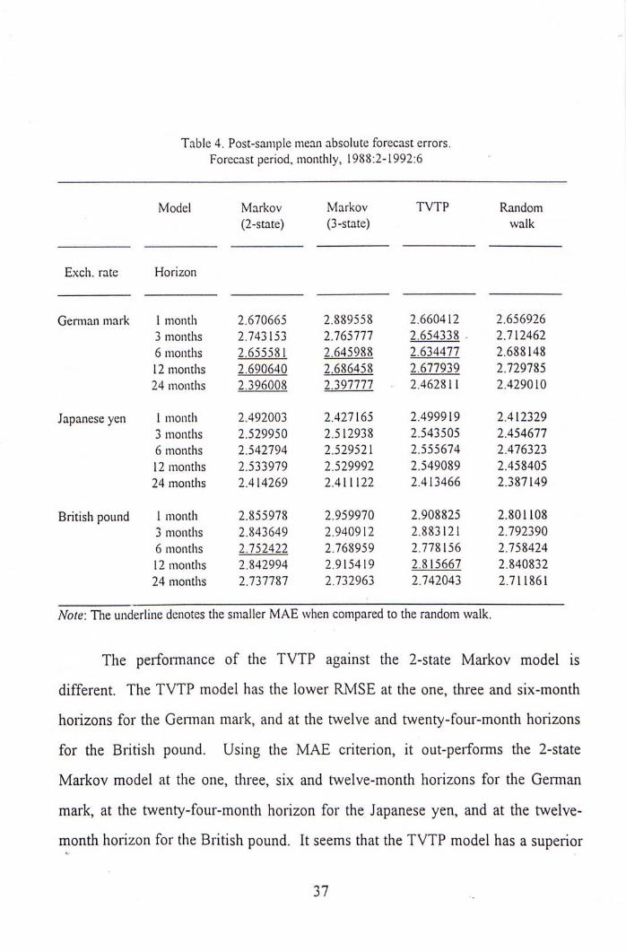
Table 4. Post -sample mean absolute forecast errors. Forecast period, monthly, 1988 :2 -1992:6 •
Model Markov Markov T V T P Random (2-state) (3-state) walk
Exch. rate Horizon
German mark 1 month 2 . 6 7 0 6 6 5 2 . 8 8 9 5 5 8 2 . 6 6 0 4 1 2 2 . 6 5 6 9 2 6 3 months 2 . 7 4 3 1 5 3 2 . 7 6 5 7 7 7 2 . 6 5 4 3 3 8 . 2 . 7 1 2 4 6 2 6 months 2 . 6 5 5 5 8 1 2 . 6 4 5 9 8 8 2 . 6 3 4 4 7 7 2 . 6 8 8 1 4 8
12 months 2 . 6 9 0 6 4 0 2 . 6 8 6 4 5 8 2 . 6 7 7 9 3 9 2 . 7 2 9 7 8 5 2 4 months 2 . 3 9 6 0 0 8 2 . 3 9 7 7 7 7 2 . 4 6 2 8 1 1 2 . 4 2 9 0 1 0
Japanese yen 1 month 2 . 4 9 2 0 0 3 2 . 4 2 7 1 6 5 2 . 4 9 9 9 1 9 2 . 4 1 2 3 2 9 3 months 2 . 5 2 9 9 5 0 2 . 5 1 2 9 3 8 2 . 5 4 3 5 0 5 2 . 4 5 4 6 7 7 6 months 2 . 5 4 2 7 9 4 2 . 5 2 9 5 2 1 2 . 5 5 5 6 7 4 2 . 4 7 6 3 2 3
12 months 2 . 5 3 3 9 7 9 2 . 5 2 9 9 9 2 2 . 5 4 9 0 8 9 2 . 4 5 8 4 0 5 2 4 months 2 . 4 1 4 2 6 9 2 . 4 1 1 1 2 2 2 . 4 1 3 4 6 6 2 . 3 8 7 1 4 9
British pound 1 month 2 . 8 5 5 9 7 8 2 . 9 5 9 9 7 0 2 . 9 0 8 8 2 5 2 . 8 0 1 1 0 8 3 months 2 . 8 4 3 6 4 9 2 . 9 4 0 9 1 2 2 . 8 8 3 1 2 1 2 . 7 9 2 3 9 0 6 months 2 . 7 5 2 4 2 2 2 . 7 6 8 9 5 9 2 . 7 7 8 1 5 6 2 . 7 5 8 4 2 4 12 months 2 . 8 4 2 9 9 4 2 . 9 1 5 4 1 9 2 . 8 1 5 6 6 7 2 . 8 4 0 8 3 2 2 4 months 2 . 7 3 7 7 8 7 2 . 7 3 2 9 6 3 2 . 7 4 2 0 4 3 2 . 7 1 1 8 6 1
Note: T h e underline denotes the smaller M A E when compared to the random walk.
The performance of the TVTP against the 2-state Markov model is
different. The TVTP model has the lower RMSE at the one, three and six-month
horizons for the German mark, and at the twelve and twenty-four-month horizons
for the British pound. Using the MAE criterion, it out-performs the 2-state
Markov model at the one, three, six and twelve-month horizons for the German
mark, at the twenty-four-month horizon for the Japanese yen, and at the twelve-
month horizon for the British pound. It seems that the TVTP model has a superior
37 .
forecasting power for the German mark, which is consistent with the large LR in
Table 1. The comparison in terms of the RMSE among the 2-state and the 3-state
Markov, the TVTP and the random walk models are also considered, and at the
one-month horizon the random walk does the best for all three currencies. At the
three-month horizon the TVTP and the random walk models do the best for one
and the remaining two currencies respectively. At the six and twelve-month
horizons the 3-state Markov, the TVTP and the random walk models perform
better for one currency individually. At the twenty-four-month horizon, the 3-state
Markov model yields more satisfactory forecasts for two currencies while the
TVTP model perfonns better for the remaining currency. Similar results are
drawn using the criterion of the MAE. At the one-month horizon the random walk
does the best for all three currencies. At the three-month horizon the TVTP and
the random walk models do the best for one and the remaining two currencies
respectively. At the six-month horizon the 2-state Markov, the TVTP and the
random walk models perform better for one currency individually. At the twelve-
month horizon the TVTP model produces more satisfactory forecasts for two
currencies while the random walk performs better for the remaining currency. At
the twenty-four-month horizon the 2-state Markov model out-performs the others
for one currency while the random walk offers more attractive prediction for the
remaining two currencies. These results show that the Markov models do not out-
perform the random walk in terms of forecasting over short horizons. To put the
picture differently, when the 2-state and the 3-state Markov and the TVTP models
are grouped together as a single entity and is compared to the random walk, it can
be observed that this entity has lower RMSE at the three, six, twelve and twenty-
four-month horizons for the German mark, at the twenty-four-month horizon for
the Japanese yen, and at the six, twelve and twenty-four-month horizons for the
British pound. Using the MAE criterion, it out-peiforms the random walk at the
38 .

three, six, twelve and twenty-four-month horizons for the German mark, at the six
and twelve-month horizons for the British pound. These results indicate that
although the Markov models as an entity offers more satisfactory forecasts for the
German mark, it is still defeated by the random walk in the contest of prediction
for the Japanese yen and the British pound.
I.
39 .

CHAPTER 6
CONCLUSION
This thesis demonstrates that the extended Markov switching models offer
better description of movement of some exchange rates in the sample than the
simple Markov switching model. For instance, the German mark is more likely to
follow a stochastic process generated by the TVTP model, while the TVTP and the
3-state Markov models delineate the Japanese yen much better. Moreover, the
TVTP model has higher out-of-sample prediction power for the German mark
while more satisfactory forecasts are given by the 3-state Markov model for the
German mark and the Japanese yen in contrast with the simple 2-state Markov
model. Nevertheless, one point should be noted that although the TVTP model is
suitable for modeling the Japanese yen in sample, it generates the poorest
forecasts. The reason may be that high variability of the estimates on the
coefficients of the transition probabilities causes the influence of the market
fundamentals ambiguous, or the coefficients may change over time as random
variables or also experience discrete shifts in regime in and out of sample. When
the contest with the random walk is considered, the results of the thesis indicate
that although the Markov models as a group have better forecasting ability for the
German mark, it is still defeated by the random walk in the contest for the
Japanese yen and the British pound, and as a whole the Markov models do not out-
perform the random walk in offering good forecasts over short horizons.
Exchange markets sometimes appear quite calm and at other times highly
volatile. Therefore, one can consider the changes in volatility over time in the
Markov-switching framework. The approach suggested by Hamilton and Susmel
(1994) is to modify the Markov model to incorporate the autoregressive
conditional heteroskedasticity (ARCH) effect. Nevertheless, some difficulties will
40 ,
be encountered that on the one hand, one must determine the lag order of the
conditional variance and the criteria for the order determination proposed by Engle
(1982) cannot be directly applied in this situation. On the other hand, the
algorithm developed by Kim (1993) cannot be adopted because this algorithm is
limited in use to the conditional density function which only depends on the
current state s , like (1),but the density function with the ARCH effect will
depend on St ’ .s^.y,....••, s . where z is the number of the lag of the conditional
variance. Therefore, these two restrictions cause estimation of the Markov model
with the ARCH effect more complicated.
One can also consider building a 3-state Markov model with time-varying
transition probabilities although the formulation is more complex since one cannot
again make use of the advantage on mathematical simplicity provided by the
logistic function for the 2-state TVTP model.
41 .
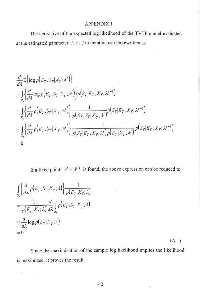
APPENDIX 1
The derivative of the expected log likelihood of the TVTP model evaluated
at the estimated parameter A at j th iteration can be rewritten as
±E[\ogp[Er.Sr\XT-xj)}
dX
二 J { 妄知 I 义一 )似‘?—丑‘厂’〜义厂 i )
二 妄 厂 ( 帖 丨 义 — — - — —
= 0
If a fixed point M = ?J'! is found, the above expression can be reduced to
二 ^ ( ^ i i y 去 知 , 知 丨 义 )
= -^\ogp[Ej\Xj\X)
aX = 0
(A. I)
Since the maximization of the sample log likelihood implies the likelihood
is maximized, it proves the result.
42 ,
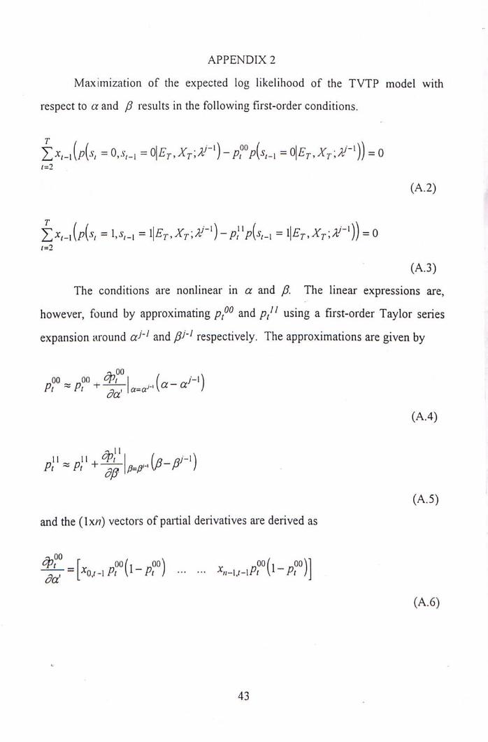
APPENDIX 2
Maximization of the expected log likelihood of the TVTP model with
respect to a and p results in the following first-order conditions.
T
2 >卜 1 ( / 7 ( 1 � = 0 ,‘ y 卜 1 二0| 五 义 广 = 0 | i r r ’ X , , ; 义 " - 1 ) ) 二 0
1=2
(A.2)
1=2
(A.3)
The conditions are nonlinear in a and p. The linear expressions are,
however, found by approximating and P t " using a first-order Taylor series
expansion around a�'丨 and p j ] respectively. The approximations are given by
„00 ”00 , Cp, j-\\ Pt h 丨 I仅一仅
(A.4)
o 1 1
Pt - A p=/}'AP-P
(A.5)
and the (Ixa?) vectors of partial derivatives are derived as
o 00 - . > / \ 1
^O.r-1 Pt [^-Pt . ^n-U-lPt V Pt I dd I- J
(A.6)
43 ,
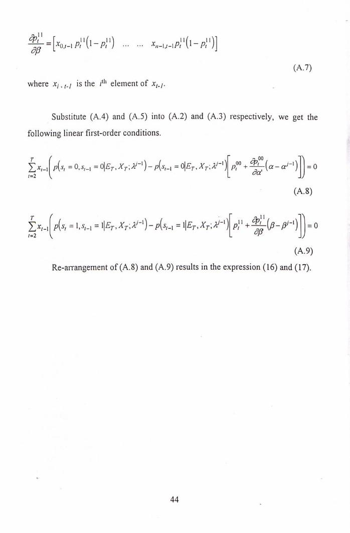
ap L J
(A.7)
where x,, is the /山 element of x .y.
Substitute (A.4) and (A.5) into (A.2) and (A.3) respectively, we get the
following linear first-order conditions.
T ( 厂 一 00 1、 厂(、.,=0,、,,_1二0|£,厂’1厂;2广1)_/7(�1=0|£厂’^>;义广1) p,oo + l ( “ _ a 广 I ) = 0
'=2 V L V
(A.8)
= U - i = 1 | 五 r , 义 丨 ) - P “ - i = 1 |五 r ’义 r ;义叫 P” + 誓 ( / ^ - 广 丨 ) 1 = 0
/=2 V L " 」)
(A.9)
Re-arrangement of (A.8) and (A.9) results in the expression (16) and (17).
44
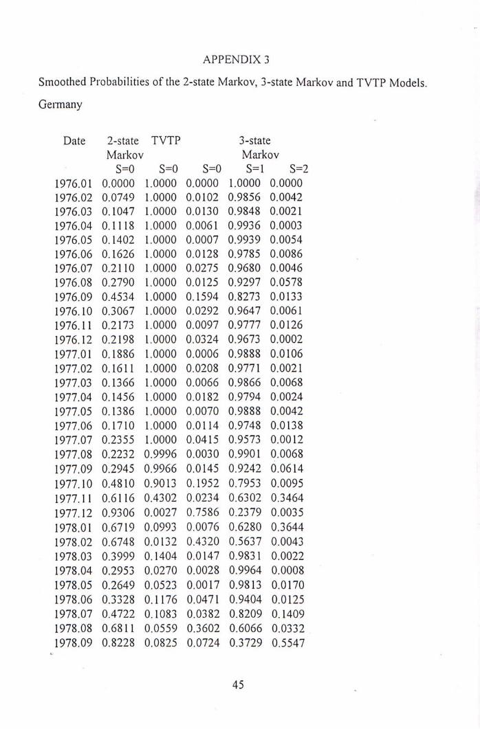
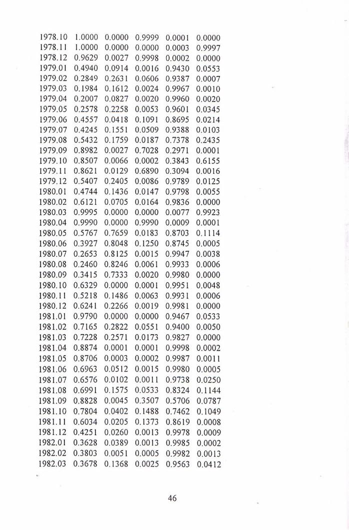
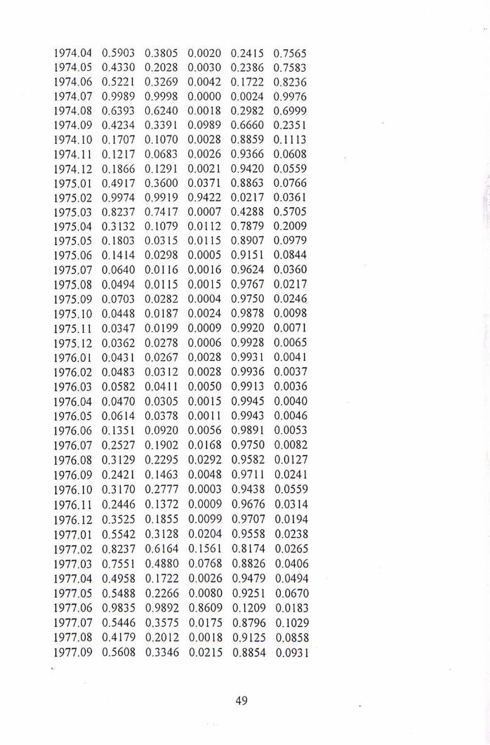
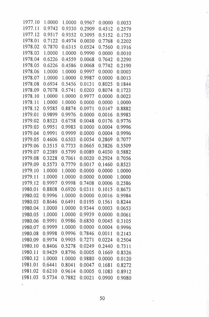
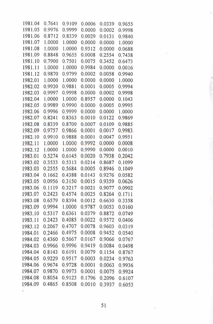
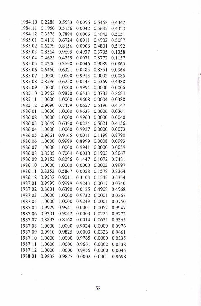
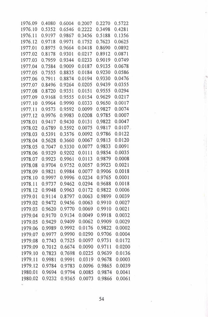
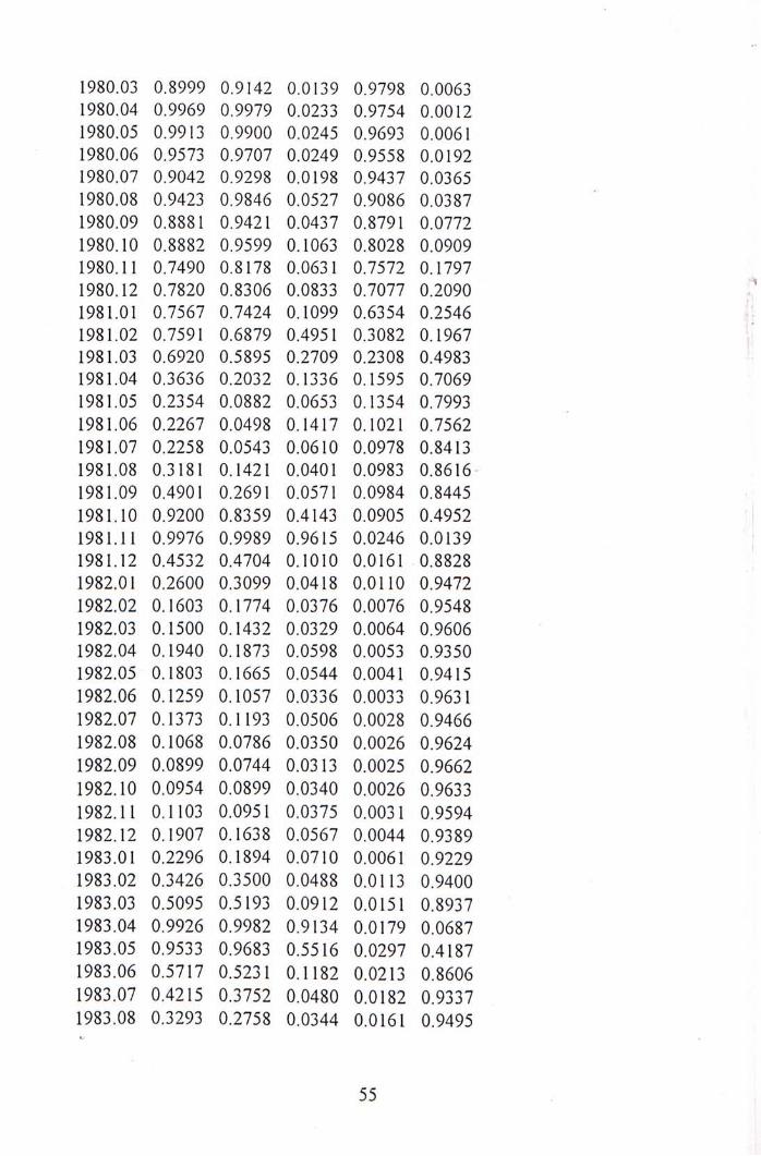
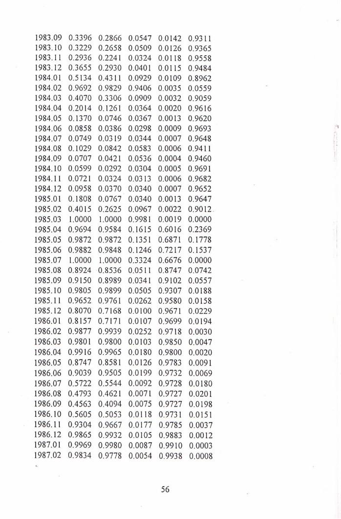
APPENDIX 3
Smoothed Probabilities of the 2-state Markov, 3-state Markov and TVTP Models.
Germany
Date 2-state TVTP 3-state Markov Markov
S = 0 S = 0 S = 0 S = 1 S=2 1976.01 0.0000 1.0000 0.0000 1.0000 0.0000 1976.02 0.0749 1.0000 0.0102 0.9856 0.0042 1976.03 0.1047 1.0000 0.0130 0.9848 0.0021 1976.04 0.1118 1.0000 0.0061 0.9936 0.0003 1976.05 0.1402 1.0000 0.0007 0.9939 0.0054 1976.06 0.1626 1.0000 0.0128 0.9785 0.0086 1976.07 0.2110 1.0000 0.0275 0.9680 0.0046 1976.08 0.2790 1.0000 0.0125 0.9297 0.0578 1976.09 0.4534 1.0000 0.1594 0.8273 0.0133 1976.10 0.3067 1.0000 0.0292 0.9647 0.0061 1976.11 0.2173 1.0000 0.0097 0.9777 0.0126 1976.12 0.2198 1.0000 0.0324 0.9673 0.0002 1977.01 0.1886 1.0000 0.0006 0.9888 0.0106 1977.02 0.1611 1.0000 0.0208 0.9771 0.0021 1977.03 0.1366 1.0000 0.0066 0.9866 0.0068 1977.04 0.1456 1.0000 0.0182 0.9794 0.0024 1977.05 0.1386 1.0000 0.0070 0.9888 0.0042 1977.06 0.1710 1.0000 0.0114 0.9748 0.0138 1977.07 0.2355 1.0000 0.0415 0.9573 0.0012 1977.08 0.2232 0.9996 0.0030 0.9901 0.0068 1977.09 0.2945 0.9966 0.0145 0.9242 0.0614 1977.10 0.4810 0.9013 0.1952 0.7953 0.0095 1977.11 0.6116 0.4302 0.0234 0.6302 0.3464 1977.12 0.9306 0.0027 0.7586 0.2379 0.0035 1978.01 0.6719 0.0993 0.0076 0.6280 0.3644 1978.02 0.6748 0.0132 0.4320 0.5637 0.0043 1978.03 0.3999 0.1404 0.0147 0.9831 0.0022 1978.04 0.2953 0.0270 0.0028 0.9964 0.0008 1978.05 0.2649 0.0523 0.0017 0.9813 0.0170 1978.06 0.3328 0.1176 0.0471 0.9404 0.0125 1978.07 0.4722 0.1083 0.0382 0.8209 0.1409 1978.08 0.6811 0.0559 0.3602 0.6066 0.0332 1978.09 0.8228 0.0825 0.0724 0.3729 0.5547
45
1978.10 1.0000 0.0000 0.9999 0.0001 0.0000 1978.11 1.0000 0.0000 0.0000 0.0003 0.9997 1978.12 0.9629 0.0027 0.9998 0.0002 0.0000 1979.01 0.4940 0.0914 0.0016 0.9430 0.0553 1979.02 0.2849 0.2631 0.0606 0.9387 0.0007 1979.03 0.1984 0.1612 0.0024 0.9967 0.0010 • 1979.04 0.2007 0.0827 0.0020 0.9960 0.0020 1979.05 0.2578 0.2258 0.0053 0.9601 0.0345 1979.06 0.4557 0.0418 0.1091 0.8695 0.0214 1979.07 0.4245 0.1551 0.0509 0.9388 0.0103 1979.08 0.5432 0.1759 0.0187 0.7378 0.2435 1979.09 0.8982 0.0027 0.7028 0.2971 0.0001 1979.10 0.8507 0.0066 0.0002 0.3843 0.6155 1979.11 0.8621 0.0129 0.6890 0.3094 0.0016 1979.12 0.5407 0.2405 0.0086 0.9789 0.0125 1980.01 0.4744 0.1436 0.0147 0.9798 0.0055 1980.02 0.6121 0.0705 0.0164 0.9836 0.0000 1980.03 0.9995 0.0000 0.0000 0.0077 0.9923 1980.04 0.9990 0.0000 0.9990 0.0009 0.0001 1980.05 0.5767 0.7659 0.0183 0.8703 0.1114 1980.06 0.3927 0.8048 0.1250 0.8745 0.0005 1980.07 0.2653 0.8125 0.0015 0.9947 0.0038 1980.08 0.2460 0.8246 0.0061 0.9933 0.0006 1980.09 0.3415 0.7333 0.0020 0.9980 0.0000 1980.10 0.6329 0.0000 0.0001 0.9951 0.0048 1980.11 0.5218 0.1486 0.0063 0.9931 0.0006 1980.12 0.6241 0.2266 0.0019 0.9981 0.0000 1981.01 0.9790 0.0000 0.0000 0.9467 0.0533 1981.02 0.7165 0.2822 0.0551 0.9400 0.0050 1981.03 0.7228 0.2571 0.0173 0.9827 0.0000 1981.04 0.8874 0.0001 0.0001 0.9998 0.0002 1981.05 0.8706 0.0003 0.0002 0.9987 0.0011 1981.06 0.6963 0.0512 0.0015 0.9980 0.0005 1981.07 0.6576 0.0102 0.0011 0.9738 0.0250 1981.08 0.6991 0.1575 0.0533 0.8324 0.1144 1981.09 0.8828 0.0045 0.3507 0.5706 0.0787 1981.10 0.7804 0.0402 0.1488 0.7462 0.1049 1981.11 0.6034 0.0205 0.1373 0.8619 0.0008 1981.12 0.4251 0.0260 0.0013 0.9978 0.0009 1982.01 0.3628 0.0389 0.0013 0.9985 0.0002 1982.02 0.3803 0.0051 0.0005 0.9982 0.0013 1982.03 0.3678 0.1368 0.0025 0.9563 0.0412
46
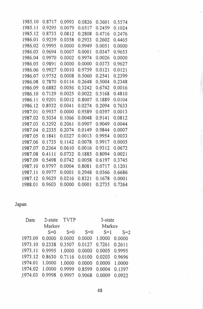
1985.10 0.8717 0.0993 0.0826 0.3601 0.5574 1985.11 0.9295 0.0079 0.6517 0.2459 0.1024 1985.12 0.8733 0.0812 0.2808 0.4716 0.2476 1986.01 0.9239 0.0358 0.2933 0.2602 0.4465 1986.02 0.9995 0.0000 0.9949 0.0051 0.0000 1986.03 0.9694 0.0007 0.0001 0.0347 0.9653 1986.04 0.9970 0.0002 0.9974 0.0026 0.0000 1986.05 0.9891 0.0000 0.0000 0.0373 0.9627 1986.06 0.9927 0.0010 0.9759 0.0121 0.0121 1986.07 0.9752 0.0008 0.5060 0.2541 0.2399 1986.08 0.7870 0.0114 0.2648 0.5004 0.2348 1986.09 0.6882 0.0056 0.3242 0.6742 0.0016 1986.10 0.7129 0.0025 0.0022 0.5168 0.4810 1986.11 0.9201 0.0012 0.8007 0.1889 0.0104 1986.12 0.8932 0.0041 0.0274 0.2094 0.7633 1987.01 0.9937 0.0000 0.9589 0.0397 0.0013 1987.02 0.5034 0.1066 0.0048 0.9141 0.0812 1987.03 0.3292 0.2061 0.0907 0.9049 0.0044 1987.04 0.2335 0.2074 0.0149 0.9844 0.0007 1987.05 0.1841 0.0327 0.0013 0.9954 0.0033 1987.06 0.1735 0.1142 0.0078 0.9917 0.0005 1987.07 0.2364 0.0610 0.0016 0.9312 0.0672 1987.08 0.4111 0.0732 0.1885 0.8094 0.0021 1987.09 0.5498 0.0742 0.0058 0.6197 0.3745 1987.10 0.9797 0.0004 0.8081 0.0717 0.1201 1987.11 0.9977 0.0001 0.2948 0.0366 0.6686 1987.12 0.9629 0.0216 0.8321 0.1678 0.0001 1988.01 0.9603 0.0000 0.0001 0.2735 0.7264
Japan
Date 2-state TVTP 3-state Markov Markov
S=0 S=0 S=0 S=1 S=2 1973.09 0.0000 0,0000 0.0000 1.0000 0.0000 1973.10 0.2338 0.3507 0.0127 0.7261 0.2611 1973.11 0.9995 1.0000 0.0000 0.0005 0.9995 1973.12 0.8630 0.7116 0.0100 0.0203 0.9696 1974.01 1.0000 1.0000 0.0000 0.0000 1.0000 1974.02 1.0000 0.9999 0.8599 0.0004 0.1397 J974.03 0.9998 0.9997 0.9068 0.0009 0.0922
48 .
1974.04 0.5903 0.3805 0.0020 0.2415 0.7565 1974.05 0.4330 0.2028 0.0030 0.2386 0.7583 1974.06 0.5221 0.3269 0.0042 0.1722 0.8236 1974.07 0.9989 0.9998 0.0000 0.0024 0.9976 1974.08 0.6393 0.6240 0.0018 0.2982 0.6999 1974.09 0.4234 0.3391 0.0989 0.6660 0.2351 1974.10 0.1707 0.1070 0.0028 0.8859 0.1113 1974.11 0.1217 0.0683 0.0026 0.9366 0.0608 1974.12 0.1866 0.1291 0.0021 0.9420 0.0559 1975.01 0.4917 0.3600 0.0371 0.8863 0.0766 1975.02 0.9974 0.9919 0.9422 0.0217 0.0361 1975.03 0.8237 0.7417 0.0007 0.4288 0.5705 1975.04 0.3132 0.1079 0.0112 0.7879 0.2009 1975.05 0.1803 0.0315 0.0115 0.8907 0.0979 1975.06 0.1414 0.0298 0.0005 0.9151 0.0844 1975.07 0.0640 0.0116 0.0016 0.9624 0.0360 1975.08 0.0494 0.0115 0.0015 0.9767 0.0217 1975.09 0.0703 0.0282 0.0004 0.9750 0.0246 1975.10 0.0448 0.0187 0.0024 0.9878 0.0098 1975.11 0.0347 0.0199 0.0009 0.9920 0.0071 1975.12 0.0362 0.0278 0.0006 0.9928 0.0065 1976.01 0.0431 0.0267 0.0028 0.9931 0.0041 1976.02 0.0483 0.0312 0.0028 0.9936 0.0037 1976.03 0.0582 0.0411 0.0050 0.9913 0.0036 1976.04 0.0470 0.0305 0.0015 0.9945 0.0040 1976.05 0.0614 0.0378 0.0011 0.9943 0.0046 1976.06 0.1351 0.0920 0.0056 0.9891 0.0053 1976.07 0.2527 0.1902 0.0168 0.9750 0.0082 1976.08 0.3129 0.2295 0.0292 0.9582 0.0127 1976.09 0.2421 0.1463 0.0048 0.9711 0.0241 1976.10 0.3170 0.2777 0.0003 0.9438 0.0559 1976.11 0.2446 0.1372 0.0009 0.9676 0.0314 1976.12 0.3525 0.1855 0.0099 0.9707 0.0194 1977.01 0.5542 0.3128 0.0204 0.9558 0.0238 1977.02 0.8237 0.6164 0.1561 0.8174 0.0265 1977.03 0.7551 0.4880 0.0768 0.8826 0.0406 1977.04 0.4958 0.1722 0.0026 0.9479 0.0494 1977.05 0.5488 0.2266 0.0080 0.9251 0.0670 1977.06 0.9835 0.9892 0.8609 0.1209 0.0183 1977.07 0.5446 0.3575 0.0175 0.8796 0.1029 1977.08 0.4179 0.2012 0.0018 0.9125 0.0858 1977.09 0.5608 0.3346 0.0215 0.8854 0.0931
49 ,
1 9 7 7 . 1 0 1 . 0 0 0 0 1 . 0 0 0 0 0 . 9 9 6 7 0 . 0 0 0 0 0 . 0 0 3 3
1 9 7 7 . 1 1 0 . 9 7 4 2 0 . 9 3 3 0 0 . 2 9 0 9 0 . 4 5 1 2 0 . 2 5 7 9
1 9 7 7 . 1 2 0 . 9 5 1 7 0 . 9 3 5 2 0 . 3 0 9 5 0 . 5 1 5 2 0 . 1 7 5 3
1 9 7 8 . 0 1 0 . 7 1 2 2 0 . 4 9 7 4 0 . 0 0 3 0 0 . 7 7 6 8 0 . 2 2 0 2
1 9 7 8 . 0 2 0 . 7 8 7 0 0 . 6 3 1 5 0 . 0 5 2 4 0 . 7 5 6 0 0 . 1 9 1 6
1 9 7 8 . 0 3 1 . 0 0 0 0 1 . 0 0 0 0 0 . 9 9 9 0 0 . 0 0 0 0 0 . 0 0 1 0 .
1 9 7 8 . 0 4 0 . 6 2 2 6 0 . 4 5 5 9 0 . 0 0 6 8 0 . 7 6 4 2 0 . 2 2 9 0
1 9 7 8 . 0 5 0 . 6 2 2 6 0 . 4 5 8 6 0 . 0 0 6 8 0 . 7 7 4 2 0 . 2 1 9 0
1 9 7 8 . 0 6 1 . 0 0 0 0 1 . 0 0 0 0 0 . 9 9 9 7 0 . 0 0 0 0 0 . 0 0 0 3
1 9 7 8 . 0 7 1 . 0 0 0 0 1 . 0 0 0 0 0 . 9 9 8 7 0 . 0 0 0 0 0 . 0 0 1 3
1 9 7 8 . 0 8 0 . 6 9 3 4 0 . 5 4 5 6 0 . 0 1 3 1 0 . 8 0 2 5 0 . 1 8 4 4
1 9 7 8 . 0 9 0 . 7 0 7 8 0 . 5 7 4 1 0 . 0 2 0 3 0 . 8 0 7 4 0 . 1 7 2 3 .
1 9 7 8 . 1 0 1 . 0 0 0 0 1 . 0 0 0 0 0 . 9 9 7 7 0 . 0 0 0 0 0 . 0 0 2 3
1 9 7 8 . 1 1 1 . 0 0 0 0 1 . 0 0 0 0 0 . 0 0 0 0 0 . 0 0 0 0 1 . 0 0 0 0
1 9 7 8 . 1 2 0 . 9 5 8 5 0 . 8 8 7 4 0 . 0 9 7 1 0 . 0 1 4 7 0 . 8 8 8 2
1 9 7 9 . 0 1 0 . 9 8 9 9 0 . 9 9 7 6 0 . 0 0 0 0 0 . 0 0 1 6 0 . 9 9 8 3
1 9 7 9 . 0 2 0 . 8 5 2 3 0 . 6 7 5 8 0 . 0 0 4 8 0 . 0 1 7 6 0 . 9 7 7 6
1 9 7 9 . 0 3 0 . 9 9 5 1 0 . 9 9 8 3 0 . 0 0 0 0 0 . 0 0 0 4 0 . 9 9 9 6
1 9 7 9 . 0 4 0 . 9 9 9 1 0 . 9 9 9 9 0 . 0 0 0 0 0 . 0 0 0 4 0 . 9 9 9 6
1979.05 0.4606 0.6503 0.0054 0.2869 0.7077 i 1 9 7 9 . 0 6 0 . 3 5 1 5 0 . 7 7 3 3 0 . 0 6 6 5 0 . 3 8 2 6 0 . 5 5 0 9 •;
1 9 7 9 . 0 7 0 . 2 3 8 9 0 . 5 7 9 9 0 . 0 0 8 9 0 . 4 0 3 0 0 . 5 8 8 2 ‘
1 9 7 9 . 0 8 0 . 3 2 2 8 0 . 7 0 6 1 0 . 0 0 2 0 0 . 2 9 2 4 0 . 7 0 5 6
1 9 7 9 . 0 9 0 . 5 5 7 3 0 . 7 7 7 9 0 . 0 0 1 7 0 . 1 4 6 0 0 . 8 5 2 3
1 9 7 9 . 1 0 1 . 0 0 0 0 1 . 0 0 0 0 0 . 0 0 0 0 0 . 0 0 0 0 1 . 0 0 0 0
1 9 7 9 . 1 1 1 . 0 0 0 0 1 . 0 0 0 0 0 . 0 0 0 0 0 . 0 0 0 0 1 . 0 0 0 0
1 9 7 9 . 1 2 0 . 9 9 9 7 0 . 9 9 9 8 0 . 7 4 0 8 0 . 0 0 0 6 0 . 2 5 8 6
1 9 8 0 . 0 1 0 . 8 8 0 8 0 . 6 9 2 0 0 . 0 3 1 1 0 . 1 0 1 5 0 . 8 6 7 3
1 9 8 0 . 0 2 0 . 9 9 9 6 1 . 0 0 0 0 0 . 0 0 0 0 0 . 0 0 1 6 0 . 9 9 8 4
1 9 8 0 . 0 3 0 . 8 6 4 6 0 . 6 4 9 1 0 . 0 1 9 5 0 . 1 5 6 1 0 . 8 2 4 4
1 9 8 0 . 0 4 1 . 0 0 0 0 1 . 0 0 0 0 0 . 9 3 4 4 0 . 0 0 0 3 0 . 0 6 5 3
1 9 8 0 . 0 5 1 . 0 0 0 0 1 . 0 0 0 0 0 . 9 9 3 9 0 . 0 0 0 0 0 . 0 0 6 1
1 9 8 0 . 0 6 0 . 9 9 9 1 0 . 9 9 8 6 0 . 6 8 5 0 0 . 0 0 4 5 0 . 3 1 0 5
1 9 8 0 . 0 7 0 . 9 9 9 9 1 . 0 0 0 0 0 . 0 0 0 0 0 . 0 0 0 4 0 . 9 9 9 6
1 9 8 0 . 0 8 0 . 9 9 9 8 0 . 9 9 9 6 0 . 7 8 4 6 0 . 0 0 1 1 0 . 2 1 4 3
1 9 8 0 . 0 9 0 . 9 9 7 4 0 . 9 9 0 5 0 . 7 2 7 1 0 . 0 2 2 4 0 . 2 5 0 4
1 9 8 0 . 1 0 0 . 8 4 0 6 0 . 5 2 7 8 0 . 0 2 4 9 0 . 2 4 4 0 0 . 7 3 1 1
1980.11 0.9429 0.8796 0.0005 0.1669 0.8326 1 9 8 0 . 1 2 1 . 0 0 0 0 1 . 0 0 0 0 0 . 9 8 8 0 0 . 0 0 0 0 0 . 0 1 2 0
1 9 8 1 . 0 1 0 . 6 4 4 1 0 . 8 0 4 1 0 . 0 0 4 7 0 . 1 6 8 1 0 . 8 2 7 2
1 9 8 1 . 0 2 0 . 6 2 1 0 0 . 9 6 1 4 0 . 0 0 0 5 0 . 1 0 8 3 0 . 8 9 1 2
1 9 8 1 . 0 3 0 . 5 7 3 4 0 . 7 8 8 2 0 . 0 0 2 1 0 . 0 9 0 0 0 . 9 0 8 0
50 ,
1 9 8 1 . 0 4 0 . 7 6 4 1 0 . 9 1 0 9 0 . 0 0 0 6 0 . 0 3 3 9 0 . 9 6 5 5
1 9 8 1 . 0 5 0 . 9 9 7 6 0 . 9 9 9 9 0.0000 0.0002 0 . 9 9 9 8
1 9 8 1 . 0 6 0 . 8 7 1 2 0 . 8 3 3 9 0 . 0 0 2 9 0 . 0 1 3 1 0 . 9 8 4 0
1 9 8 1 . 0 7 1 . 0 0 0 0 1 . 0 0 0 0 0 . 0 0 0 0 0 . 0 0 0 0 1 . 0 0 0 0
1 9 8 1 . 0 8 1 . 0 0 0 0 1 . 0 0 0 0 0 . 9 3 1 2 0 . 0 0 0 0 0 . 0 6 8 8
1 9 8 1 . 0 9 0 . 8 8 4 8 0 . 9 6 5 5 0 . 0 0 0 8 0 . 2 5 5 4 0 . 7 4 3 8
1 9 8 1 . 1 0 0 . 7 9 0 0 0 . 7 5 0 1 0 . 0 0 7 5 0 . 3 4 5 2 0 . 6 4 7 3
1 9 8 1 . 1 1 1 . 0 0 0 0 1 . 0 0 0 0 0 . 9 9 8 4 0 . 0 0 0 0 0 . 0 0 1 6
1 9 8 1 . 1 2 0 . 9 8 7 0 0 . 9 7 9 9 0 . 0 0 0 2 0 . 0 0 5 8 0 . 9 9 4 0
1 9 8 2 . 0 1 1 . 0 0 0 0 1 . 0 0 0 0 0 . 0 0 0 0 0 . 0 0 0 0 1 . 0 0 0 0 ‘
1 9 8 2 . 0 2 0 . 9 9 2 0 0 . 9 8 8 1 0 . 0 0 0 1 0 . 0 0 0 5 0 . 9 9 9 4
1 9 8 2 . 0 3 0 . 9 9 9 7 0 . 9 9 9 8 0 . 0 0 0 0 0 . 0 0 0 2 0 . 9 9 9 8
1 9 8 2 . 0 4 1 . 0 0 0 0 1 . 0 0 0 0 0 . 8 9 5 7 0 . 0 0 0 0 0 . 1 0 4 3
1 9 8 2 . 0 5 0 . 9 9 8 9 0 . 9 9 9 0 0 . 0 0 0 0 0 . 0 0 0 5 0 . 9 9 9 5
1 9 8 2 . 0 6 0 . 9 9 9 6 0 . 9 9 9 9 0 . 0 0 0 0 0 . 0 0 0 0 1 . 0 0 0 0
1 9 8 2 . 0 7 0 . 8 2 4 1 0 . 8 3 6 3 0 . 0 0 1 0 0 . 0 1 2 2 0 . 9 8 6 9
1 9 8 2 . 0 8 0 . 8 3 3 9 0 . 8 7 0 9 0 . 0 0 0 7 0 . 0 1 0 9 0 . 9 8 8 5
1 9 8 2 . 0 9 0 . 9 7 5 7 0 . 9 8 6 6 0 . 0 0 0 1 0 . 0 0 1 7 0 . 9 9 8 3
1 9 8 2 . 1 0 0 . 9 9 1 0 0 . 9 8 8 8 0 . 0 0 0 1 0 . 0 0 4 7 0 . 9 9 5 1
1982.11 1.0000 1.0000 0.9992 0.0000 0.0008 i 1 9 8 2 . 1 2 1 . 0 0 0 0 1 . 0 0 0 0 0 . 9 9 9 0 0 . 0 0 0 0 0 . 0 0 1 0 ‘;
1 9 8 3 . 0 1 0 . 5 2 7 4 0 . 6 1 4 5 0 . 0 0 2 0 0 . 7 9 3 8 0 . 2 0 4 2
1 9 8 3 . 0 2 0 . 3 5 3 3 0 . 5 3 1 3 0 . 0 2 1 4 0 . 8 6 8 7 0 . 1 0 9 9
1 9 8 3 . 0 3 0 . 2 5 5 5 0 . 5 6 8 4 0 . 0 0 0 5 0 . 8 9 4 6 0 . 1 0 4 9
1 9 8 3 . 0 4 0 . 1 6 6 2 0 . 4 3 8 8 0 . 0 1 4 3 0 . 9 2 7 6 0 . 0 5 8 2
1 9 8 3 . 0 5 0 . 0 9 5 6 0 . 3 1 5 0 0 . 0 0 1 5 0 . 9 3 5 9 0 . 0 6 2 6
1 9 8 3 . 0 6 0 . 1 1 1 9 0 . 3 2 1 7 0 . 0 0 2 1 0 . 9 0 7 7 0 . 0 9 0 2
1 9 8 3 . 0 7 0 . 2 4 2 3 0 . 4 5 7 4 0 . 0 0 2 5 0 . 8 2 6 4 0 . 1 7 1 1
1 9 8 3 . 0 8 0 . 6 5 7 9 0 . 8 3 9 4 0 . 0 0 1 2 0 . 6 6 3 0 0 . 3 3 5 8
1 9 8 3 . 0 9 0 . 9 9 9 4 1 . 0 0 0 0 0 . 9 7 8 7 0 . 0 0 5 3 0 . 0 1 6 0
1 9 8 3 . 1 0 0 . 5 3 1 7 0 . 6 3 6 1 0 . 0 3 7 9 0 . 8 8 7 2 0 . 0 7 4 9
1 9 8 3 . 1 1 0 . 2 4 2 3 0 . 4 0 8 5 0 . 0 0 2 2 0 . 9 5 7 2 0 . 0 4 0 6
1 9 8 3 . 1 2 0 . 2 0 6 7 0 . 4 7 0 7 0 . 0 0 7 8 0 . 9 6 0 3 0 . 0 3 1 9
1 9 8 4 . 0 1 0 . 2 4 6 6 0 . 4 9 7 5 0 . 0 0 0 8 0 . 9 4 5 2 0 . 0 5 4 0
1 9 8 4 . 0 2 0 . 4 3 6 0 0 . 5 6 6 7 0 . 0 1 6 7 0 . 9 0 6 6 0 . 0 7 6 7
1 9 8 4 . 0 3 0 . 9 9 6 6 0 . 9 9 9 6 0 . 9 4 1 9 0 . 0 0 8 4 0 . 0 4 9 8
1 9 8 4 . 0 4 0 . 8 1 4 3 0 . 6 1 9 1 0 . 0 0 7 9 0 . 1 1 5 4 0 . 8 7 6 7
1 9 8 4 . 0 5 0 . 9 2 2 9 0 . 9 5 1 7 0 . 0 0 0 3 0 . 0 2 3 4 0 . 9 7 6 3
1 9 8 4 . 0 6 0 . 9 6 7 4 0 . 9 7 2 8 0 . 0 0 0 1 0 . 0 0 6 3 0 . 9 9 3 6
1 9 8 4 . 0 7 0 . 9 8 7 0 0 . 9 9 7 3 0 . 0 0 0 1 0 . 0 0 7 5 0 . 9 9 2 4
1984.08 0.8054 0.9123 0.1796 0.2096 0.6107 1 9 8 4 . 0 9 0 . 4 8 6 5 0 . 8 5 0 8 0 . 0 0 1 0 0 . 3 9 3 7 0 . 6 0 5 3
f.
51 .
1 9 8 4 . 1 0 0 . 2 2 8 8 0 . 5 5 8 3 0 . 0 0 9 6 0 . 5 4 6 2 0 . 4 4 4 2
1 9 8 4 . 1 1 0 . 1 9 5 0 0 . 5 1 5 6 0 . 0 0 4 2 0 . 5 6 3 5 0 . 4 3 2 3
1 9 8 4 . 1 2 0 . 3 3 7 8 0 . 7 8 9 4 0 . 0 0 0 6 0 . 4 9 4 3 0 . 5 0 5 1
1 9 8 5 . 0 1 0 . 4 1 1 8 0 . 6 7 2 4 0 . 0 0 1 1 0 . 4 9 0 2 0 . 5 0 8 7
1 9 8 5 . 0 2 0 . 6 2 7 9 0 . 8 1 5 6 0 . 0 0 0 8 0 . 4 8 0 1 0 . 5 1 9 2
1 9 8 5 . 0 3 0 . 8 5 6 4 0 . 9 6 9 5 0 . 4 9 3 7 0 . 3 7 0 5 0 . 1 3 5 8 •
1 9 8 5 . 0 4 0 . 4 6 2 5 0 . 4 2 5 9 0 . 0 0 7 1 0 . 8 7 7 2 0 . 1 1 5 7
1 9 8 5 . 0 5 0 . 4 2 0 0 0 . 3 6 9 8 0 . 0 0 4 6 0 . 9 0 8 9 0 . 0 8 6 5
1 9 8 5 . 0 6 0 . 6 4 6 0 0 . 6 3 2 1 0 . 0 4 8 5 0 . 8 5 5 1 0 . 0 9 6 4
1 9 8 5 . 0 7 1 . 0 0 0 0 1 . 0 0 0 0 0 . 9 9 1 3 0 . 0 0 0 2 0 . 0 0 8 5 ‘
1 9 8 5 . 0 8 0 . 8 5 9 6 0 . 6 2 5 8 0 . 0 1 4 3 0 . 5 3 6 9 0 . 4 4 8 8
1 9 8 5 . 0 9 1 . 0 0 0 0 1 . 0 0 0 0 0 . 9 9 9 4 0 . 0 0 0 0 0 . 0 0 0 6 ‘
1 9 8 5 . 1 0 0 . 9 9 6 2 0 . 9 8 7 0 0 . 6 5 3 3 0 . 0 7 8 3 0 . 2 6 8 4
1 9 8 5 . 1 1 1 . 0 0 0 0 1 . 0 0 0 0 0 . 9 6 0 8 0 . 0 0 0 4 0 . 0 3 8 8
1 9 8 5 . 1 2 0 . 9 0 9 0 0 . 7 4 7 9 0 . 0 6 5 7 0 . 5 1 9 6 0 . 4 1 4 7
1 9 8 6 . 0 1 1 . 0 0 0 0 1 . 0 0 0 0 0 . 9 6 3 3 0 . 0 0 0 6 0 . 0 3 6 1
1 9 8 6 . 0 2 1 . 0 0 0 0 1 . 0 0 0 0 0 . 9 9 6 0 0 . 0 0 0 0 0 . 0 0 4 0
1 9 8 6 . 0 3 0 . 8 6 4 9 0 . 6 3 2 0 0 . 0 2 2 4 0 . 5 6 2 1 0 . 4 1 5 6
1 9 8 6 . 0 4 1 . 0 0 0 0 1 . 0 0 0 0 0 . 9 9 2 7 0 . 0 0 0 0 0 . 0 0 7 3
1 9 8 6 . 0 5 0 . 9 6 6 1 0 . 9 1 6 5 0 . 0 0 1 1 0 . 1 1 9 9 0 . 8 7 9 0
1 9 8 6 . 0 6 1 . 0 0 0 0 0 . 9 9 9 9 0 . 8 9 9 9 0 . 0 0 0 8 0 . 0 9 9 3 ;
1 9 8 6 . 0 7 1 . 0 0 0 0 1 . 0 0 0 0 0 . 9 9 4 1 0 . 0 0 0 0 0 . 0 0 5 9 ‘
1 9 8 6 . 0 8 0 . 8 5 0 5 0 . 7 0 0 4 0 . 0 0 3 0 0 . 1 9 0 3 0 . 8 0 6 7
1986.09 0.9153 0.8286 0.1447 0.1072 0.7481 1 9 8 6 . 1 0 1 . 0 0 0 0 1 . 0 0 0 0 0 . 0 0 0 0 0 . 0 0 0 3 0 . 9 9 9 7
1 9 8 6 . 1 1 0 . 8 3 5 3 0 . 5 8 6 7 0 . 0 0 5 8 0 . 1 5 7 8 0 . 8 3 6 4
1 9 8 6 . 1 2 0 . 9 5 3 2 0 . 9 0 1 1 0 . 3 1 0 3 0 . 1 5 4 3 0 . 5 3 5 4
1 9 8 7 . 0 1 0 . 9 9 9 9 0 . 9 9 9 9 0 . 9 2 4 3 0 . 0 0 1 7 0 . 0 7 4 0
1 9 8 7 . 0 2 0 . 8 6 0 1 0 . 6 3 9 0 0 . 0 1 2 5 0 . 4 9 0 8 0 . 4 9 6 8
1 9 8 7 . 0 3 1 . 0 0 0 0 1 . 0 0 0 0 0 . 9 7 3 2 0 . 0 0 0 1 0 . 0 2 6 7
1 9 8 7 . 0 4 1 . 0 0 0 0 1 . 0 0 0 0 0 . 9 2 4 9 0 . 0 0 0 1 0 . 0 7 5 0
1 9 8 7 . 0 5 0 . 9 9 2 9 0 . 9 9 4 1 0 . 0 0 0 1 0 . 0 0 5 2 0 . 9 9 4 7
1 9 8 7 . 0 6 0 . 9 2 0 1 0 . 9 0 4 2 0 . 0 0 0 3 0 . 0 2 2 5 0 . 9 7 7 2
1987.07 0.8893 0.8168 0.0014 0.0621 0.9365 1 9 8 7 . 0 8 1 . 0 0 0 0 1 . 0 0 0 0 0 . 9 0 2 4 0 . 0 0 0 0 0 . 0 9 7 6
1 9 8 7 . 0 9 0 . 9 9 1 0 0 . 9 8 2 5 0 . 0 0 0 3 0 . 0 3 3 6 0 . 9 6 6 1
1 9 8 7 . 1 0 1 . 0 0 0 0 1 . 0 0 0 0 0 . 9 7 6 5 0 . 0 0 0 0 0 . 0 2 3 5
1 9 8 7 . 1 1 1 . 0 0 0 0 1 . 0 0 0 0 0 . 9 6 6 1 0 . 0 0 0 2 0 . 0 3 3 8
1 9 8 7 . 1 2 1 . 0 0 0 0 1 . 0 0 0 0 0 . 9 9 5 5 0 . 0 0 0 0 0 . 0 0 4 5
1 9 8 8 . 0 1 0 . 9 8 3 2 0 . 9 8 7 7 0 . 0 0 0 2 0 . 0 3 0 1 0 . 9 6 9 8
I.
52 .
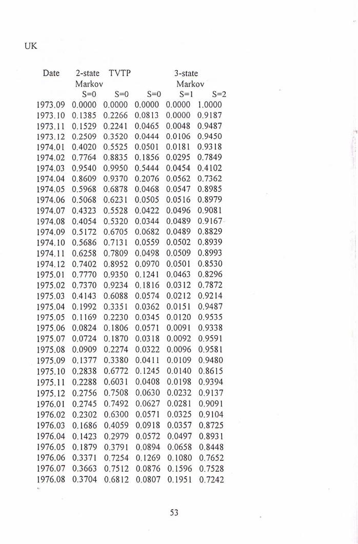
UK
Date 2-state TVTP 3-state Markov Markov
S=0 S=0 S=0 S=1 S=2 ‘ 1973.09 0.0000 0.0000 0.0000 0.0000 1.0000 1973.10 0.1385 0.2266 0.0813 0.0000 0.9187 1 9 7 3 . 1 1 0 . 1 5 2 9 0 . 2 2 4 1 0 . 0 4 6 5 0 . 0 0 4 8 0 . 9 4 8 7 气
1973.12 0.2509 0.3520 0.0444 0.0106 0.9450 ‘ 1 9 7 4 . 0 1 0 . 4 0 2 0 0 . 5 5 2 5 0 . 0 5 0 1 0 . 0 1 8 1 0 . 9 3 1 8 :
1974.02 0.7764 0.8835 0.1856 0.0295 0.7849 1974.03 0.9540 0.9950 0.5444 0.0454 0.4102 1974.04 0.8609 0.9370 0.2076 0.0562 0.7362 1974.05 0.5968 0.6878 0.0468 0.0547 0.8985 1974.06 0.5068 0.6231 0.0505 0.0516 0.8979 1974.07 0.4323 0.5528 0.0422 0.0496 0.9081 1974.08 0.4054 0.5320 0.0344 0.0489 0.9167 1974.09 0.5172 0.6705 0.0682 0.0489 0.8829 1974.10 0.5686 0.7131 0.0559 0.0502 0.8939 i 1 9 7 4 . 1 1 0 . 6 2 5 8 0 . 7 8 0 9 0 . 0 4 9 8 0 . 0 5 0 9 0 . 8 9 9 3 :
1974.12 0.7402 0.8952 0.0970 0.0501 0.8530 1975.01 0.7770 0.9350 0.1241 0.0463 0.8296 1975.02 0.7370 0.9234 0.1816 0.0312 0.7872 1975.03 0.4143 0.6088 0.0574 0.0212 0.9214 1975.04 0.1992 0.3351 0.0362 0.0151 0.9487 1975.05 0.1169 0.2230 0.0345 0.0120 0.9535 1975.06 0.0824 0.1806 0.0571 0.0091 0.9338 1975.07 0.0724 0.1870 0.0318 0.0092 0.9591 1975.08 0.0909 0.2274 0.0322 0.0096 0.9581 1975.09 0.1377 0.3380 0.0411 0.0109 0.9480 1975.10 0.2838 0.6772 0.1245 0.0140 0.8615 1975.11 0.2288 0.6031 0.0408 0.0198 0.9394 1975.12 0.2756 0.7508 0.0630 0.0232 0.9137 1976.01 0.2745 0.7492 0.0627 0.0281 0.9091 1976.02 0.2302 0.6300 0.0571 0.0325 0.9104 1976.03 0.1686 0.4059 0.0918 0.0357 0.8725 1976.04 0.1423 0.2979 0.0572 0.0497 0.8931 1976.05 0.1879 0.3791 0.0894 0.0658 0.8448 1976.06 0.3371 0.7254 0.1269 0.1080 0.7652 1976.07 0.3663 0.7512 0.0876 0.1596 0.7528 1 9 7 6 . 0 8 0 . 3 7 0 4 0 . 6 8 1 2 0 . 0 8 0 7 0 . 1 9 5 1 0 . 7 2 4 2
t.
53 .
1 9 7 6 . 0 9 0 . 4 0 8 0 0 . 6 0 0 4 0 . 2 0 0 7 0 . 2 2 7 0 0 . 5 7 2 2
1 9 7 6 . 1 0 0 . 5 3 5 2 0 . 6 5 4 6 0 . 2 2 2 2 0 . 3 4 9 8 0 . 4 2 8 1
1 9 7 6 . 1 1 0 . 9 1 9 7 0 . 9 8 6 7 0 . 3 4 5 6 0 . 5 1 8 8 0 . 1 3 5 6
1 9 7 6 . 1 2 0 . 9 7 1 8 0 . 9 9 7 1 0 . 1 7 5 2 0 . 7 6 2 3 0 . 0 6 2 5
1 9 7 7 . 0 1 0 . 8 9 7 5 0 . 9 6 6 4 0 . 0 4 1 8 0 . 8 6 9 0 0 . 0 8 9 2
1 9 7 7 . 0 2 0 . 8 1 7 8 0 . 9 3 0 1 0 . 0 2 1 7 0 . 8 9 1 2 0 . 0 8 7 1
1 9 7 7 . 0 3 0 . 7 9 5 9 0 . 9 3 4 4 0 . 0 2 3 3 0 . 9 0 1 9 0 . 0 7 4 9
1 9 7 7 . 0 4 0 . 7 5 8 4 0 . 9 0 0 9 0 . 0 1 8 7 0 . 9 1 3 5 0 . 0 6 7 8
1 9 7 7 . 0 5 0 . 7 5 5 5 0 . 8 8 3 5 0 . 0 1 8 4 0 . 9 2 3 0 0 . 0 5 8 6
1 9 7 7 . 0 6 0 . 7 9 1 1 0 . 8 8 7 4 0 . 0 1 9 4 0 . 9 3 3 0 0 . 0 4 7 6 ‘
1 9 7 7 . 0 7 0 . 8 4 9 6 0 . 9 2 6 4 0 . 0 2 0 5 0 . 9 4 3 9 0 . 0 3 5 5
1 9 7 7 . 0 8 0 . 8 7 2 0 0 . 9 3 5 1 0 . 0 1 5 1 0 . 9 5 5 5 0 . 0 2 9 4 ‘
1 9 7 7 . 0 9 0 . 9 1 6 8 0 . 9 5 5 5 0 . 0 1 5 4 0 . 9 6 2 9 0 . 0 2 1 7
1 9 7 7 . 1 0 0 . 9 9 6 4 0 . 9 9 9 0 0 . 0 3 3 3 0 . 9 6 5 0 0 . 0 0 1 7
1 9 7 7 . 1 1 0 . 9 5 7 3 0 . 9 5 9 2 0 . 0 0 9 9 0 . 9 8 2 7 0 . 0 0 7 4
1 9 7 7 . 1 2 0 . 9 9 7 6 0 . 9 9 8 3 0 . 0 2 0 8 0 . 9 7 8 5 0 . 0 0 0 7
1 9 7 8 . 0 1 0 . 9 4 1 7 0 . 9 4 3 0 0 . 0 1 3 1 0 . 9 8 2 2 0 . 0 0 4 7
1 9 7 8 . 0 2 0 . 6 7 8 9 0 . 5 5 9 2 0 . 0 0 7 5 0 . 9 8 1 7 0 . 0 1 0 7 .
1 9 7 8 . 0 3 0 . 5 3 9 1 0 . 3 5 7 6 0 . 0 0 9 2 0 . 9 7 8 6 0 . 0 1 2 2
1 9 7 8 . 0 4 0 . 5 6 2 8 0 . 3 6 6 0 0 . 0 0 6 7 0 . 9 8 1 3 0 . 0 1 2 0 |
1 9 7 8 . 0 5 0 . 7 0 4 7 0 . 5 3 3 0 0 . 0 0 7 7 0 . 9 8 3 3 0 . 0 0 9 1 ;
1 9 7 8 . 0 6 0 . 9 3 2 9 0 . 9 2 0 2 0 . 0 1 1 1 0 . 9 8 5 4 0 . 0 0 3 5
1 9 7 8 . 0 7 0 . 9 9 2 3 0 . 9 9 6 1 0 . 0 1 1 3 0 . 9 8 7 9 0 . 0 0 0 8
1 9 7 8 . 0 8 0 . 9 7 0 4 0 . 9 7 5 2 0 . 0 0 5 7 0 . 9 9 2 3 0 . 0 0 2 1
1 9 7 8 . 0 9 0 . 9 8 2 1 0 . 9 9 8 4 0 . 0 0 7 7 0 . 9 9 0 6 0 . 0 0 1 8
1978.10 0.9997 0.9996 0.0234 0.9765 0.0001 1 9 7 8 . 1 1 0 . 9 7 3 7 0 . 9 4 6 2 0 . 0 2 9 4 0 . 9 6 8 8 0 . 0 0 1 8
1 9 7 8 . 1 2 0 . 9 9 4 8 0 . 9 9 6 3 0 . 0 1 7 2 0 . 9 8 2 2 0 . 0 0 0 6
1 9 7 9 . 0 1 0 . 9 1 1 4 0 . 8 7 9 7 0 . 0 0 6 3 0 . 9 8 9 9 0 . 0 0 3 9
1 9 7 9 . 0 2 0 . 9 4 7 2 0 . 9 4 5 6 0 . 0 0 6 3 0 . 9 9 1 0 0 . 0 0 2 7
1 9 7 9 . 0 3 0 . 9 6 2 0 0 . 9 7 7 0 0 . 0 0 6 9 0 . 9 9 1 0 0 . 0 0 2 1
1 9 7 9 . 0 4 0 . 9 1 7 0 0 . 9 1 3 4 0 . 0 0 4 9 0 . 9 9 1 8 0 . 0 0 3 2
1 9 7 9 . 0 5 0 . 9 4 2 9 0 . 9 4 0 9 0 . 0 0 6 2 0 . 9 9 0 9 0 . 0 0 2 9
1 9 7 9 . 0 6 0 . 9 9 8 9 0 . 9 9 9 2 0 . 0 1 7 6 0 . 9 8 2 2 0 . 0 0 0 2
1 9 7 9 . 0 7 0 . 9 9 7 7 0 . 9 9 9 0 0 . 0 2 9 0 0 . 9 7 0 6 0 . 0 0 0 4
1 9 7 9 . 0 8 0 . 7 7 4 3 0 . 7 5 2 5 0 . 0 0 9 7 0 . 9 7 3 1 0 . 0 1 7 2
1 9 7 9 . 0 9 0 . 7 0 1 2 0 . 6 6 7 4 0 . 0 0 9 0 0 . 9 7 1 1 0 . 0 2 0 0
1 9 7 9 . 1 0 0 . 7 8 2 3 0 . 7 6 9 8 0 . 0 2 2 5 0 . 9 6 3 9 0 . 0 1 3 6
1 9 7 9 . 1 1 0 . 9 9 8 1 0 . 9 9 9 1 0 . 0 3 1 9 0 . 9 6 7 8 0 . 0 0 0 3
1979.12 0.9784 0.9783 0.0096 0.9865 0.0039 1 9 8 0 . 0 1 0 . 9 6 9 4 0 . 9 7 9 4 0 . 0 0 8 5 0 . 9 8 7 4 0 . 0 0 4 1
1 9 8 0 . 0 2 0 . 9 2 3 2 0 . 9 3 6 5 0 . 0 0 7 3 0 . 9 8 6 6 0 . 0 0 6 1 ••
54 .
1 9 8 0 . 0 3 0 . 8 9 9 9 0 . 9 1 4 2 0 . 0 1 3 9 0 . 9 7 9 8 0 . 0 0 6 3
1 9 8 0 . 0 4 0 . 9 9 6 9 0 . 9 9 7 9 0 . 0 2 3 3 0 . 9 7 5 4 0 . 0 0 1 2
1 9 8 0 . 0 5 0 . 9 9 1 3 0 . 9 9 0 0 0 . 0 2 4 5 0 . 9 6 9 3 0 . 0 0 6 1
1 9 8 0 . 0 6 0 . 9 5 7 3 0 . 9 7 0 7 0 . 0 2 4 9 0 . 9 5 5 8 0 . 0 1 9 2
1 9 8 0 . 0 7 0 . 9 0 4 2 0 . 9 2 9 8 0 . 0 1 9 8 0 . 9 4 3 7 0 . 0 3 6 5
1 9 8 0 . 0 8 0 . 9 4 2 3 0 . 9 8 4 6 0 . 0 5 2 7 0 . 9 0 8 6 0 . 0 3 8 7 ‘
1 9 8 0 . 0 9 0 . 8 8 8 1 0 . 9 4 2 1 0 . 0 4 3 7 0 . 8 7 9 1 0 . 0 7 7 2
1 9 8 0 . 1 0 0 . 8 8 8 2 0 . 9 5 9 9 0 . 1 0 6 3 0 . 8 0 2 8 0 . 0 9 0 9
1 9 8 0 . 1 1 0 . 7 4 9 0 0 . 8 1 7 8 0 . 0 6 3 1 0 . 7 5 7 2 0 . 1 7 9 7
1 9 8 0 . 1 2 0 . 7 8 2 0 0 . 8 3 0 6 0 . 0 8 3 3 0 . 7 0 7 7 0 . 2 0 9 0 ‘
1 9 8 1 . 0 1 0 . 7 5 6 7 0 . 7 4 2 4 0 . 1 0 9 9 0 . 6 3 5 4 0 . 2 5 4 6
1 9 8 1 . 0 2 0 . 7 5 9 1 0 . 6 8 7 9 0 . 4 9 5 1 0 . 3 0 8 2 0 . 1 9 6 7 •
1 9 8 1 . 0 3 0 . 6 9 2 0 0 . 5 8 9 5 0 . 2 7 0 9 0 . 2 3 0 8 0 . 4 9 8 3
1 9 8 1 . 0 4 0 . 3 6 3 6 0 . 2 0 3 2 0 . 1 3 3 6 0 . 1 5 9 5 0 . 7 0 6 9
1 9 8 1 . 0 5 0 . 2 3 5 4 0 . 0 8 8 2 0 . 0 6 5 3 0 . 1 3 5 4 0 . 7 9 9 3
1 9 8 1 . 0 6 0 . 2 2 6 7 0 . 0 4 9 8 0 . 1 4 1 7 0 . 1 0 2 1 0 . 7 5 6 2
1 9 8 1 . 0 7 0 . 2 2 5 8 0 . 0 5 4 3 0 . 0 6 1 0 0 . 0 9 7 8 0 . 8 4 1 3
1 9 8 1 . 0 8 0 . 3 1 8 1 0 . 1 4 2 1 0 . 0 4 0 1 0 . 0 9 8 3 0 . 8 6 1 6
1 9 8 1 . 0 9 0 . 4 9 0 1 0 . 2 6 9 1 0 . 0 5 7 1 0 . 0 9 8 4 0 . 8 4 4 5
1 9 8 1 . 1 0 0 . 9 2 0 0 0 . 8 3 5 9 0 . 4 1 4 3 0 . 0 9 0 5 0 . 4 9 5 2 !
1 9 8 1 . 1 1 0 . 9 9 7 6 0 . 9 9 8 9 0 . 9 6 1 5 0 . 0 2 4 6 0 . 0 1 3 9
1 9 8 1 . 1 2 0 . 4 5 3 2 0 . 4 7 0 4 0 . 1 0 1 0 0 . 0 1 6 1 0 . 8 8 2 8
1 9 8 2 . 0 1 0 . 2 6 0 0 0 . 3 0 9 9 0 . 0 4 1 8 0 . 0 1 1 0 0 . 9 4 7 2
1 9 8 2 . 0 2 0 . 1 6 0 3 0 . 1 7 7 4 0 . 0 3 7 6 0 . 0 0 7 6 0 . 9 5 4 8
1 9 8 2 . 0 3 0 . 1 5 0 0 0 . 1 4 3 2 0 . 0 3 2 9 0 . 0 0 6 4 0 . 9 6 0 6
1 9 8 2 . 0 4 0 . 1 9 4 0 0 . 1 8 7 3 0 . 0 5 9 8 0 . 0 0 5 3 0 . 9 3 5 0
1 9 8 2 . 0 5 0 . 1 8 0 3 0 . 1 6 6 5 0 . 0 5 4 4 0 . 0 0 4 1 0 . 9 4 1 5
1 9 8 2 . 0 6 0 . 1 2 5 9 0 . 1 0 5 7 0 . 0 3 3 6 0 . 0 0 3 3 0 . 9 6 3 1
1 9 8 2 . 0 7 0 . 1 3 7 3 0 . 1 1 9 3 0 . 0 5 0 6 0 . 0 0 2 8 0 . 9 4 6 6
1 9 8 2 . 0 8 0 . 1 0 6 8 0 . 0 7 8 6 0 . 0 3 5 0 0 . 0 0 2 6 0 . 9 6 2 4
1 9 8 2 . 0 9 0 . 0 8 9 9 0 . 0 7 4 4 0 . 0 3 1 3 0 . 0 0 2 5 0 . 9 6 6 2
1 9 8 2 . 1 0 0 . 0 9 5 4 0 . 0 8 9 9 0 . 0 3 4 0 0 . 0 0 2 6 0 . 9 6 3 3
1 9 8 2 . 1 1 0 . 1 1 0 3 0 . 0 9 5 1 0 . 0 3 7 5 0 . 0 0 3 1 0 . 9 5 9 4
1 9 8 2 . 1 2 0 . 1 9 0 7 0 . 1 6 3 8 0 . 0 5 6 7 0 . 0 0 4 4 0 . 9 3 8 9
1 9 8 3 . 0 1 0 . 2 2 9 6 0 . 1 8 9 4 0 . 0 7 1 0 0 . 0 0 6 1 0 . 9 2 2 9
1 9 8 3 . 0 2 0 . 3 4 2 6 0 . 3 5 0 0 0 . 0 4 8 8 0 . 0 1 1 3 0 . 9 4 0 0
1 9 8 3 . 0 3 0 . 5 0 9 5 0 . 5 1 9 3 0 . 0 9 1 2 0 . 0 1 5 1 0 . 8 9 3 7
1 9 8 3 . 0 4 0 . 9 9 2 6 0 . 9 9 8 2 0 . 9 1 3 4 0 . 0 1 7 9 0 . 0 6 8 7
1 9 8 3 . 0 5 0 . 9 5 3 3 0 . 9 6 8 3 0 . 5 5 1 6 0 . 0 2 9 7 0 . 4 1 8 7
1 9 8 3 . 0 6 0 . 5 7 1 7 0 . 5 2 3 1 0 . 1 1 8 2 0 . 0 2 1 3 0 . 8 6 0 6
1 9 8 3 . 0 7 0 . 4 2 1 5 0 . 3 7 5 2 0 . 0 4 8 0 0 . 0 1 8 2 0 . 9 3 3 7
1983.08 0.3293 0.2758 0.0344 0.0161 0.9495 t.
55
1983.09 0.3396 0.2866 0.0547 0.0142 0.9311 1983.10 0.3229 0.2658 0.0509 0.0126 0.9365 1983.11 0.2936 0.2241 0.0324 0.0118 0.9558 1983.12 0.3655 0.2930 0.0401 0.0115 0.9484 1984.01 0.5134 0.4311 0.0929 0.0109 0.8962 1984.02 0.9692 0.9829 0.9406 0.0035 0.0559 ‘ 1984.03 0.4070 0.3306 0.0909 0.0032 0.9059 1984.04 0.2014 0.1261 0.0364 0.0020 0.9616 1984.05 0.1370 0.0746 0.0367 0.0013 0.9620 1984.06 0.0858 0.0386 0.0298 0.0009 0.9693 �
1984.07 0.0749 0.0319 0.0344 0,0007 0.9648 1984.08 0.1029 0.0842 0.0583 0.0006 0.9411 ‘ 1984.09 0.0707 0.0421 0.0536 0.0004 0.9460 1984.10 0.0599 0.0292 0.0304 0.0005 0.9691 1984.11 0.0721 0.0324 0.0313 0.0006 0.9682 1984.12 0.0958 0.0370 0.0340 0.0007 0.9652 1985.01 0.1808 0.0767 0.0340 0.0013 0.9647 1985.02 0.4015 0.2625 0.0967 0.0022 0.9012 1985.03 1.0000 1.0000 0.9981 0.0019 0.0000 1985.04 0.9694 0.9584 0.1615 0.6016 0.2369 | 1985.05 0.9872 0.9872 0.1351 0.6871 0.1778 \ 1985.06 0.9882 0.9848 0.1246 0.7217 0.1537 1985.07 1.0000 1.0000 0.3324 0.6676 0.0000 1 9 8 5 . 0 8 0 . 8 9 2 4 0 . 8 5 3 6 0 . 0 5 1 1 0 . 8 7 4 7 0 . 0 7 4 2
1985.09 0.9150 0.8989 0.0341 0.9102 0.0557 1985.10 0.9805 0.9899 0.0505 0.9307 0.0188 1985.11 0.9652 0.9761 0.0262 0.9580 0.0158 1985.12 0.8070 0.7168 0.0100 0.9671 0.0229 1986.01 0.8157 0.7171 0.0107 0.9699 0.0194 1986.02 0.9877 0.9939 0.0252 0.9718 0.0030 1986.03 0.9801 0.9800 0.0103 0.9850 0.0047 1986.04 0.9916 0.9965 0.0180 0.9800 0.0020 1 9 8 6 . 0 5 0 . 8 7 4 7 0 . 8 5 8 1 0 . 0 1 2 6 0 . 9 7 8 3 0 . 0 0 9 1
1986.06 0.9039 0.9505 0.0199 0.9732 0.0069 1986.07 0.5722 0.5544 0.0092 0.9728 0.0180 1986.08 0.4793 0.4621 0.0071 0.9727 0.0201 1986.09 0.4563 0.4094 0.0075 0.9727 0.0198 1986.10 0.5605 0.5053 0.0118 0.9731 0.0151 1986.11 0.9304 0.9667 0.0177 0.9785 0.0037 1986.12 0.9865 0.9932 0.0105 0.9883 0.0012 1987.01 0.9969 0.9980 0.0087 0.9910 0.0003 1987.02 0.9834 0.9778 0.0054 0.9938 0.0008
56 ,
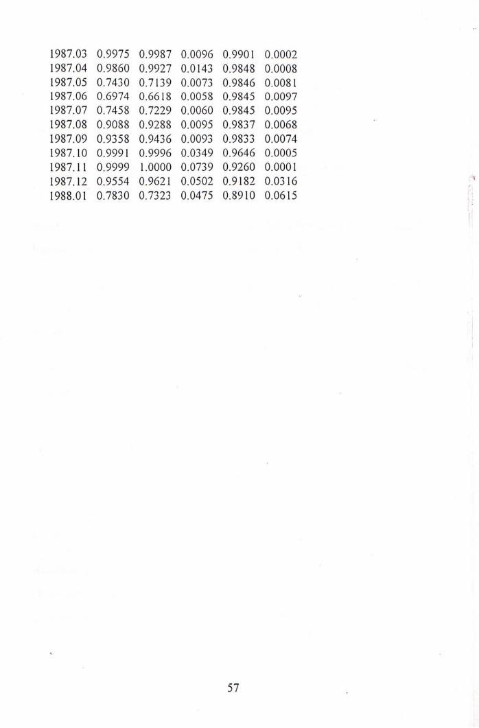
1987.03 0.9975 0.9987 0.0096 0.9901 0.0002 1987.04 0.9860 0.9927 0.0143 0.9848 0.0008 1987.05 0.7430 0.7139 0.0073 0.9846 0.0081 1987.06 0.6974 0.6618 0.0058 0.9845 0.0097 1987.07 0.7458 0.7229 0.0060 0.9845 0.0095 1987.08 0.9088 0.9288 0.0095 0.9837 0.0068 ‘ 1987.09 0.9358 0.9436 0.0093 0.9833 0.0074 1987.10 0.9991 0.9996 0.0349 0.9646 0.0005 1987.11 0.9999 1.0000 0.0739 0.9260 0.0001 1987.12 0.9554 0.9621 0.0502 0.9182 0.0316 ^ 1988.01 0.7830 0.7323 0.0475 0.8910 0.0615
i
57 .
BIBLIOGRAPHY
Diebold, F. X., J. H. Lee and G. C. Weinbach (1994),"Regime Switching with
Time-Varying Transition Probabilities", in C. Hargreaves, ed.,Nonstationary Time
Series Analysis and Cointegration. Oxford: Oxford University Press.
Dombusch, R. (1976), "Expectations and Exchange Rate Dynamics", Journal of
Political Economy, Vol. 84’ pp. 1161-1176.
Engel, C. (1994), "Can the Markov Switching Model Forecast Exchange Rates?",
Journal of International Economics, Vol. 36’ pp. 151-165.
Engel, C. aad J. D. Hamilton (1990), "Long Swings in the Dollar: Are They in the
Data and Do Markets Know it?", The American Economic Review, Vol. 80, No.4,
pp. 689-713.
Engle, R. F. (1982), "Autoregressive Conditional Heteroskedasticity with
Estimates of the Variance of United Kingdom Inflation", Econometrica, Vol. 50,
pp. 987-1007.
Filardo, A. J. (1994), "Business-Cycle Phases and Their Transitional Dynamics",
Journal of Business and Economic Statistics, Vol. 12, No. 3,pp. 299-308.
Goodwin, T. H. (1993), "Business-Cycle Analysis with a Markov-Switching
Model", Journal of Business and Economic Statistics, Vol. 11’ No. 3’ pp. 331-339.
Hamilton, J. D. (1988), "Rational Expectations Econometric Analysis of Changes
in Regime: An Investigation of the Term Structure of Interest Rates", Journal of
Economic Dynamics and Control. Vol. 12, pp. 385-423.
t.
58
(1990), "Analysis of Time Series Subject to Changes in Regime", Journal
of Econometrics, Vol. 45, pp. 39-70.
(1993), "Estimation, Inference and Forecasting of Time Series Subject to
Changes in Regime", in G. S. Maddala, C. R. Rao and H. D. Vinod, eds.’
Handbook of Statistics. Vol. 11’ pp. 231-260.
.1、
Hamilton, J. D. and R. Susmel (1994), "Autoregressive Conditional •
Heteroskedasticity and Changes in Regime", Journal of Econometrics. Vol. 64,pp.
307-333.
Kaminsky, G. (1993), "Is There a Peso Problem? Evidence from the Dollar/Pound
Exchange Rate, 1976-1987", The American Economic Review, Vol. 83, No. 3, pp.
450-472. “
Kim, C. J. (1994), "Dynamic Linear Models with Markov-switching", Journal of
Econometrics,Vol. 60, pp. 1-22.
Meese, R. A. and K. Rogoff (1983), "Empirical Exchange Rate Models of the
Seventies. Do they fit out of sample?", Journal of International Economics. Vol.
14,pp. 3-24.
59 .

.. 1
•
.
广
-
坎
;
1
1 *
4 1 44.
.
:,
,
‘
:
:
^ i
,
.
.
.
•
.
.
........
: >
.
. *
•
•
\
. .5
-
,
»
- .
,
•
.
.
--
• •
.
.r
•
.
.
.
.
"
f
:.」 .
.•
-
.
:
/
. .
二
丨
-
.
1 -If /
- •
•
.
•{
•
i.!!
I
.
•
, •
‘ «
: • I
•
- t •
•
. .ir-
•
!
*»,
——

<M
CUHK Libraries
DDD733flbfl