1

Vitaly Bychkov

Examples on use of

vector analysis in physics

Institute of Physics, Umeå University

2003

2

Contents

1. Vector functions, fields 4

1.1 A moving particle 4

1.2 Fields in fluid mechanics. Streamlines 4

1.3 Fields in electrodynamics 5

2. Derivatives and integrals of vector functions 5

2.1 Electric force on distributed charge 5

2.2 Gravitational force on distributed mass 5

3. Gradient 6

3.1 Particle motion in a potential field 6

4. Line integrals 7

4.1 Work of a force 7

4.2 Work of a gravitational force 7

4.3 Electric force on charge distributed along a wire 7

4.4 Magnetic force on a wire with current 8

5. Surface integrals 8

5.1 Volumetric flow rate (discharge) of a fluid 8

5.2 Mass flux in fluid mechanics 10

5.3 Electric current 10

5.4 Heat flux due to thermal conduction 11

5.5 Diffusion 12

5.6 Pressure force in a fluid 13

5.7 Faraday’s law in electrodynamics 14

6. Divergence. The Gauss theorem. Continuity equations 14

6.1 Incompressible flow 14

6.2 Coulomb’s law in electrostatics 15

6.3 The Poisson equation for the gravitational force 16

6.4 Incompressible flow with sources 17

6.5 Mass conservation in fluid mechanics 17

6.6 Conservation of electric charge 18

3

6.7 Collective drift of particles 19

6.8 Heat transfer in a flow 21

6.9 Density variations for a fluid parcel 22

7. Rotor. The Stokes theorem 23

7.1 Faraday’s law 23

7.2 Magnetic field of currents in electrostatics 24

7.3 Charge conservation and the Maxwell equations 25

7.4 Rotor in fluid mechanics. Vorticity 25

7.5 Vector potential in fluid mechanics 26

8. Nabla operator 27

8.1 Electromagnetic waves in vacuum 27

9. Other integral theorems 29

9.1 Hydrostatics 29

9.2 The Archimedes force 31

9.3 Force on a magnetic dipole 31

4

1. Vector functions, fields

1.1 A moving particle

Position of a particle in space is determined by the position vector )(trr . The particle

velocity and acceleration are specified by the formulas

dt

drv ,

2

2

dt

d ra . (1.1)

1.2 Fields in fluid mechanics. Streamlines.

Fluid motion is usually described with the help of the scalar fields of pressure

),( tPP r , density ),( tr , temperature ),( tTT r , and a vector field of the flow

velocity ),( truu . The velocity field may be depicted by use of streamlines. By

definition, a tangent unit vector to a streamline τ points in the direction of velocity u .

Calculating a unit tangent vector as

dr

drτ with ),,( dzdydxdr

we find

udr

d urτ ,

that is

u

u

dr

dx x , u

u

dr

dy y,

u

u

dr

dz z

or

zyx u

dz

u

dy

u

dx. (1.2)

In the same way we can calculate field-lines for other vector fields.

Example: Find stream-lines of the flow ),(),( xyuu yx .

We have to solve the equation

x

dy

y

dx, or 0dyydxx .

We find

5

constyx 22 .

The streamlines are circles.

1.3 Fields in electrodynamics

In electrodynamics we work with the scalar fields of potential ),( tr , and charge

density ),( tee r . The most important vector fields used in electrodynamics are the

electric field ),( trEE , the magnetic field ),( trBB and the current density ),( trjj .

2. Derivatives and integrals of vector functions

2.1 Electric force on distributed charge

Electric charge distributed in space is described with the help of charge density

dV

dqe , (2.1)

which determines elementary charge in the position r as

dzdydxdVdq ee )(r .

Example: The charge is placed in the electric field )(rEE . What is the total force

acting on the charge inside some volume 0V ?

Solution:

The force acting on the elementary charge is

dVdqd eEEF . (2.2)

Then the total force is calculated as

0V

e dVdqd EEFF . (2.3)

2.2 Gravitational force on distributed mass

Mass distribution inside a star with the gravitational field )(rgg is described by the

density

dV

dM

6

The gravitational field is, actually, the gravitational acceleration. What is the total force

acting on the mass inside some volume 0V ?

Solution:

The force acting on the elementary mass dVdM is

dVdMd ggF . (2.4)

Then the total force is calculated as

0V

dVdMd ggFF . (2.5)

3. Gradient

3.1 Particle motion in a potential field

A particle of mass m moves with velocity v in a potential field with force )(rF .

Show that total particle energy 2

2

1mv is a constant.

Solution:

Particle motion is described by Newton’s law

Fv

dt

dm .

Multiplying both parts of the equation by the particle velocity dt

drv

dt

d

dt

d

dt

dm

rF

rvv

we find

dt

dmv

dt

d 2

2

1, that is 0

2

1 2mvdt

d

or constmv2

2

1.

7

4. Line integrals

4.1 Work of a force

A particle moving from a point P to a point Q along a curve L experiences a force F ,

which is not necessarily a potential one. What is the total work of the force?

Solution:

The elementary work is rF ddW . Then the total work is

L

Q

P

ddWW rF .

4.2 Work of a gravitational force

What is the total work of the gravitational force when we move the mass m along a line

L ascending by the total height z ? The gravity acceleration is constant ),0,0( gg .

Solution:

The gravitational force is mmgF , where the potential rg or gz .

Then the work of the gravitational force is

zmgmdmdW PQ

LL

)(rrF .

4.3 Electric force on charge distributed along a wire

Electric charge distributed along a wire is described with the help of the line charge

density

dl

dql .

A charged wire is placed in an electric field )(rEE . What is the total force acting on

the charge? The shape of the wire is described by a curve L.

Solution:

The force acting on the elementary charge is

dldqd lEEF .

Then the total force is calculated as

L

l dldqd EEFF .

8

4.4 Magnetic force on a wire with current

A wire with current I is placed in a magnetic field )(rBB . What is the total force

acting on the charge? The shape of the wire is described by a curve L.

Solution:

The force acting on the current element rId of the wire is determined by Ampere’s law

BrF dId ,

here and below we are working in the SI units. Then the total force is calculated as

L

dId BrFF . (4.1)

5. Surface integrals

5.1 Volumetric flow rate (discharge) of a fluid.

We have a uniform flow of a fluid with velocity 1U in a tube with cross-sectional area 1S ,

see Fig. 4.1. How much fluid comes into the tank per unit time?

Solution:

The amount of the fluid coming into the tank is determined by the volume of the cylinder

with the tube cross-section at the bottom, 1S , and the height dtU1 , hence

dtUSdV 11 ,

Fig. 4.1. Fluid comes into the tank and leaves the tank: illustration of the discharge.

S1 S2

U1 dt U2 dt

flux in flux out

9

Fig. 4.2. Discharge through an arbitrary surface area.

which determines the volumetric flow rate

11USdt

dV.

In the case of an arbitrary surface and an arbitrary flow ),( truu we can divide the

surface area into elements dSd nS ˆ , where n is the normal unit vector, see Fig. 4.2.

Then the elementary fluid volume passing Sd per unit time is determined by the local

velocity of the flow ),( truu

Su ddtdV dS )()( or Su ddt

dV

dS

. (5.1)

The total discharge (the volume of the fluid passing through 0S per unit time) is

0S

ddt

dVSu . (5.2)

If the surface 0S is closed, then Eq. (5.2) specify the discharge of the fluid going out of

the volume enveloped by 0S , since conventionally the normal unit vector n points out .

This holds even if locally the fluid flows into the volume, because in that case 0Su d .

V0, S0

u

dS

u dt

n n

10

5.2 Mass flux in fluid mechanics.

We have an arbitrary surface 0S and an arbitrary flow ),( truu . What is the mass flux

through 0S (how much mass passes 0S per unit time)?

Solution:

We cut 0S into small surface elements Sd . Fluid volume passing through a surface

element Sd per unit time is determined by the elementary discharge Eq. (5.1). Then the

elementary mass flux is determined by the volume dSdV )( and the fluid density

Su ddtdVdM dSdS )()( , (5.3)

or

Su ddt

dM

dS

, (5.4)

and the total mass flux is

0S

ddt

dMSu . (5.5)

Similar calculations may be performed for the momentum and energy fluxes.

s

5.3 Electric current.

How can we find the electric current through a surface 0S if we know charge distribution

),( tee r and the microscopic motion of charged particles ),( truu .

Solution:

By definition, electric current I through 0S is charge passing the surface per unit time

0)/( SdtdqI . We start with the simplest case of the current produced by particles of one

type. Similar to the mass flux in fluid mechanics, the charge passing the elementary

surface Sd per unit time is determined by the particles inside the elementary volume

dSdV )( , that is

Su ddtdVdq edSedS )()( , (5.6)

and

Su ddt

dqdI e

dS

dS)( . (5.7)

11

Then we calculate the total current as

0S

e ddt

dqI Su . (5.8)

The above calculations are used to define the current density ),( trj :

Sj ddI dS)( , or

0S

dI Sj , (5.9)

which relates the current density to the microscopic parameters

uj e . (5.10)

Now let us consider the general case of different types of particles contributing to the

current, as it takes place in plasma or an electrolyte. In that case the charge density is

determined by different particles

eiie dqdVdV

dq 1, (5.11)

and the elementary current is

SuSj ddt

dq

dt

dqdI iei

dS

i

dS

dS)( , (5.12)

which reduces to the formula for the current density

ieiuj . (5.13)

5.4 Heat flux due to thermal conduction.

Suppose that we have two adjacent gas volumes at equal uniform pressure and different

temperatures, 21 TT . If we put the volumes into contact, then after some time the gas

temperature will be uniform and equal some intermediate value *T with 2

*

1 TTT .

The temperature variation imply that energy has been redistributed, though we had no

hydrodynamic motion (pressure was constant and there was no force, which could make

the gas move). In that case the energy was redistributed by use of random thermal motion

of gas particles. Physical processes related to the random motion are called transport

processes. The most important transport processes are thermal conduction, diffusion and

viscosity. In this example we consider heat flux due to thermal conduction. How much

12

heat H (thermal energy) passes through a surface 0S because of thermal conduction if

the temperature field is ),( tTT r ?

Solution:

First we consider heat flux through the elementary surface Sd . In order to describe the

heat flux we introduce the flux density similar to the current density Eq. (5.9) as

Sj ddt

dHH

dS

. (5.14)

It has been obtained experimentally that the flux density is proportional to the

temperature gradient

THj ; (5.15)

equation (5.15) is known as Fick’s law. The minus sign comes to Eq. (5.15) because heat

is transferred from the regions of larger temperature to the cold regions. The factor is

called the coefficient of thermal conduction. Then the elementary heat flux is

SdTdt

dH

dS

, (5.16)

and the total flux is

00 SS

H dTddt

dHSSj . (5.17)

5.5 Diffusion.

Another example of a transport process is diffusion. Suppose that we have a large

volume filled by a gas a in mechanic equilibrium. Besides, somewhere in the volume we

have a little amount of gas b , which does not disturb the equilibrium (for example,

particles of smoke or perfume in the air). The amount of gas b may be described by

concentration ),( tcc r , which is the number of particles b in elementary volume

dV

dNc b . (5.18)

How can we describe flux of gas b through a surface 0S due to thermal motion?

13

Solution:

In order to describe flux through an elementary surface Sd we introduce the flux density

Sj ddt

dND

dS

b , (5.19)

where the flux density is related to the concentration gradient according to Fick’s law

cDDj . (5.20)

The relation like (5.20) is typical for all transport processes. The factor D in Eq. (5.20) is

the diffusion coefficient. Then the elementary flux of gas b is

SdcDdt

dN

dS

b , (5.21)

which results in the total flux

0S

b dcDdt

dNS . (5.22)

5.6 Pressure force in a fluid.

What is the pressure force produced by a fluid on a surface area 0S ?

Solution:

By definition, pressure is a force per unit surface area directed normally to the surface.

Choosing a surface element Sd we have the elementary pressure force

SF dPd . (5.23)

The minus sign comes to Eq. (5.23) because the normal unit vector to the surface is

traditionally directed towards the fluid, but the pressure force acts in the opposite

direction. Then the total pressure force is

0S

dP SF . (5.24)

Respectively, if we are interested in torque, then we calculate first the elementary torque

)( SrFrT dPdd

and find the total torque by integration

00 SS

dPd SrFrT . (5.25)

14

5.7 Faraday’s law in electrodynamics.

Faraday’s law is another important example on use of line and surface integrals.

According to the Faraday’s law, time variation of a magnetic field generates rotational

electric field. From the mathematical point of view it implies that circulation of electric

field E along any closed loop C is proportional to time variations of the magnetic flux

through any surface S surrounded by the loop. The numerical coefficient in the law

depends on the system of units; In the SI units we have

0SC

dt

d SBrE . (5.26)

6. Divergence. The Gauss theorem. Continuity equations.

6.1 Incompressible flow.

We have an incompressible flow, for which fluid (gas) density does not change

const . What is the differential equation for the velocity field ),( truu ?

Solution:

We consider a closed arbitrary volume 0V in the stream with neither sources nor sinks.

Since the fluid density does not change, then amount of the fluid (measured by volume)

coming into 0V per unit time is equal to the amount of the fluid going out. In that case

taking into account Eq. (5.2) we have

0

0S

ddt

dVSu . (6.1)

Using the Gauss theorem we transform Eq. (6.1) into a volume integral

00

0VS

dVd uSu . (6.2)

Since the volume 0V is arbitrary, then

0u . (6.3)

15

6.2 Coulomb’s law in electrostatics.

We have two point charges Q and q separated by the distance r . According to

Coulomb’s law the force acting on q is

rr

qQeF ˆ

4 2

0

, (6.4)

where re is the unit vector pointing from Q to q , and 0 is a universal physical constant

introduced in in the SI. The electric filed is defined in electrostatics as the force acting on

unit charge

rr

Q

qe

FE ˆ

4 2

0

. (6.5)

Let us calculate the electric flux out of a sphere rS with the centre in Q and radius r .

The surface element of such a sphere is dSdSd renS ˆˆ . Then we have

0

2

2

0

2

0

2

0

2

0

44444

Qr

r

QS

r

QdS

r

QdS

r

Qd r

SSS rrr

SE . (6.6)

We can formulate the same result in a more general way for an arbitrary closed surface

0S (this result is proved rigorously in vector analysis)

0

0

000 V

eSinside

S

dVQ

dSE . (6.7)

The result Eq. (6.7) may be also presented in a differential form. With the help of the

Gauss law we transform (6.7) as

0000V

e

VS

dVdVd ESE . (6.8)

Since the volume 0V is arbitrary, then

0

eE . (6.9)

Equation (6.9) is known as the Poisson equation, and it is considered as one of the basic

results in electrodynamics.

A similar equation may be written for the magnetic field taking into account that

there are no magnetic charges

0B . (6.10)

16

6.3 The Poisson equation for the gravitational force.

Newton’s gravitational law has a form similar to Coulomb’s law in electrostatics, Eq.

(6.4)

rr

mMeF ˆ

2, (6.11)

where m and M are two point masses separated by the distance r , and is the

gravitational constant. We have the minus sign in Eq. (6.11) because two masses attract

each other, while two positive charges repulse. The gravity acceleration plays the role of

intensity of the gravitational field

rr

M

me

Fg ˆ

2. (6.12)

Calculating flux of g out of a sphere with a centre in M , we obtain

Mrr

MS

r

MdS

r

MdS

r

Md r

SSS rrr

44 2

2222Sg . (6.13)

In general, the same result may be presented as

0

0

0

44V

Sinside

S

dVMdSg . (6.14)

Using the Gauss theorem we can present the same law in the differential form

4g . (6.15)

6.4 Incompressible flow with sources.

The equation (6.3) for an incompressible flow changes, if we have sources of the fluid

(gas), for example, due to chemical reactions or because of pumps. Suppose that the

sources are distributed in an arbitrary volume 0V with the density W and produce new

fluid volume at the volumetric rate (discharge) dtdVQ / so that

0V

dVWQ . (6.16)

Then the amount of fluid leaving 0V is equal

00 VS

dVdQdt

dVuSu , (6.17)

where we have taken into account Eq. (5.2). Comparing (6.16), (6.17) we obtain

17

00 VV

dVWdVQ u .

Since the volume 0V is arbitrary, then the velocity field obeys the equation

Wu . (6.18)

6.5 Mass conservation in fluid mechanics.

We consider a flow described by the fields ),( truu , ),( tr and an arbitrary fixed

volume 0V like that shown in Fig. 4.2. Mass conservation for the chosen volume may be

described by an equation

volume) theinside variation(mass

(sources) volume) theofout flux (mass . (6.19)

Total mass inside 0V is

0V

dVM , (6.20)

which varies in time as

00 VV

dVt

dVtt

M

dt

dM, (6.21)

since the volume is fixed. We calculate mass flux out of 0V according to Eq. (5.5) and use

the Gauss theorem

00

)(flux todue VS

dVddt

dMuSu . (6.22)

Sources of mass (for example, pumps) with distributed source density ),( tWM r produce

0sources todue V

M dVWdt

dM. (6.23)

Substituting (6.21) – (6.23) into (6.19) we find

0 00

)(V V

M

V

dVWdVdVt

u . (6.24)

Since the volume 0V is arbitrary, then we obtain the differential equation of mass

conservation

18

MWt

)( u . (6.25)

If there are no sources (which is, actually, the most typical case), then Eq. (6.25) takes the

form

0)( ut

. (6.26)

Equation (6.26) is known as the continuity equation. If the fluid is incompressible

const , then the continuity equation reduces to 0u , that is to Eq. (6.3).

6.6 Conservation of electrical charge.

Similar to the previous example, we consider the fields of charge density ),( tee r ,

current density ),( trjj , and an arbitrary fixed volume 0V like that shown in Fig. 4.2.

Charge conservation for the chosen volume may be described by an equation

volume) theinside variation(charge

volume) theofout flux (charge . (6.27)

Charge variation inside 0V is

00 V

e

V

e dVt

dVtt

q

dt

dq, (6.28)

Charge flux out of the volume is determined by the electric current according to Eq. (5.8)

00

out

flux todue VS

dVdIdt

dqjSj . (6.29)

Then we find from Eq. (6.27)

00 VV

e dVdVt

j ,

which may be reduced to the differential equation of charge conservation

0jt

e . (6.30)

From the microscopic point of view in the case of one type of particles we have uj e

and the equation of charge conservation may be written in the same form as the

continuity equation

19

0)( uee

t. (6.31)

6.7 Collective drift of particles.

In this example we consider conservation of the number of particles described by

concentration, Eq. (5.18). Problems of this type are typical for combustion, where we

have to take into account concentration of fuel, oxidizer, final and intermediate products

of the reaction. In plasma physics and space science we also deal with a large number of

different particles: electrons, ions of different type, neutrals, positrons, etc. As before, we

consider a fixed volume 0V shown in Fig. 4.2. Still, in the present example we may have

particle flux caused by two different mechanisms: hydrodynamic flow and diffusion. We

start with the hydrodynamic flow with no diffusion.

a) Drift due to a flow, no diffusion

The total number of particles b in 0V is

0V

b dVcN , (6.32)

which varies in time as

00 VV

b dVt

cdVc

tt

N. (6.33)

The continuity equation for the particle drift is

volume) theinside of (variation bN

(sources) volume) theofout of(flux bN . (6.34)

Neglecting diffusion we have the flux due to the hydrodynamic flow only, which may be

calculated similar to the mass flux, Eqs. (5.3) – (5.5)

00

)(flux todue VS

b dVcdcdt

dNuSu . (6.35)

When we consider continuity of different particles, then sources and sinks are quite

typical. The number of particles of one type may change because of chemical reactions,

ionization, recombination, birth and annihilation of electron-positron pairs, etc.

Designating the density of sources/sinks by NW , we find

20

0sources todue V

Nb dVW

dt

dN. (6.36)

Using Eq. (6.34) we obtain the continuity equation for the number of particles

000

)(V

N

VV

dVWdVcdVt

cu , (6.37)

or

NWct

c)( u . (6.38)

The continuity equation holds for any type of particles.

b) Drift due to diffusion, no flow

In that case the flux out of 0V in Eq. (6.34) is determined by the diffusion only, that is

00

)(flux todue VS

b dVcDdcDdt

dNS , (6.39)

see Eq. (5.22). Substituting Eqs. (6.33), (6.36), (6.39) into Eq. (6.34), we find the

diffusion equation

000

)(V

N

VV

dVWdVcDdVt

c,

which may be presented in the differential form as

NWcDt

c)( . (6.40)

Finally, when both hydrodynamic flow and diffusion are important, then the equation of

particle drift takes into account both processes

NWcDct

c)()( u . (6.41)

6.8 Heat transfer in a flow.

How can we describe heat transfer in a flow ),( truu by a differential equation taking

into account thermal conduction?

Solution:

We consider an arbitrary fixed volume 0V shown in Fig. 4.2. The energy balance for the

volume is

21

flow) the todueflux (heat volume) theinsideiation (heat var

(sources))conduction thermal the todueflux (heat . (6.42)

Elementary heat inside dV is determined by temperature dVTCdH H , where HC is

specific heat per unit mass (which may be taken constant in many problems) and the

combination TCH plays the role of heat density. Then total heat inside 0V is

0V

H dVTCH , (6.43)

with

0

)(V

H dVTCtdt

dH. (6.44)

Heat flux due to the hydrodynamic flow is similar to the mass flux, Eq. (5.5)

00

)( todue V

H

S

H dVTCdTCdt

dHuSu

u

. (6.45)

Heat flux due to thermal conduction is given by Eq. (5.17)

00

)( todue VS

dVTdTdt

dHSu . (6.46)

In order to describe heat sources we introduce the source density HW

0sources todue V

H dVWdt

dH. (6.47)

Then the equation of heat transfer may be presented as

0 000

)()()(V V

H

V

H

V

H dVWdVTdVTCdVTCt

u , (6.48)

or

HHH WTTCTCt

)()()( u . (6.49)

In the simple case of no flow 0u , constant density const , constant coefficient of

thermal conduction const and no sources, the above equation reduces to the well-

known equation of thermal conduction

TCt

T

H

2. (6.50)

22

6.9 Density variations for a fluid parcel.

The approach of fields deals with parameters defined in a fixed reference frame, e.g.

),( tr , ),( truu . In that case the derivatives

t

, t

u

define time variation of density (velocity) in a fixed point. How can we find density

variations dt

d for a fluid parcel moving together with the flow?

Solution:

Suppose that the parcel trajectory is )(trr . Then the dependence ),( tr is

reduced to a function of one variable ]),([ ttr , and we have

dt

d

tdt

d r.

By definition

ur

dt

d,

which leads to

utdt

d. (6.51)

The equation (6.51) is known as substantive (hydrodynamic) derivative. Using the

substantive derivative we can calculate the acceleration of a fluid parcel. Applying (6.51)

to all components of the fluid velocity we find

xxx ut

u

dt

du)(u ,

and similar expressions for yu , zu . Multiplying the obtained expressions by xe , ye , ze ,

respectively, and taking the sum we find the acceleration

uuuu

)(tdt

d. (6.52)

23

7. Rotor. The Stokes theorem.

7.1 Faraday’s law.

Reduce Faraday’s law, Eq. (5.26), to a differential equation.

Solution:

The right-hand side of Faraday’s law

0SC

dt

d SBrE

may be transformed by use of the Stokes theorem as

0

)(SC

dd SErE ,

which leads to

00

)(SS

dt

d SBSE .

Since the surface 0S is arbitrary, then we can present Faraday’s law in the form

t

BE . (7.1)

In the stationary case (in electrostatics) we have

0t

B and, hence, 0E ,

which implies that the electric field in electrostatics is potential.

7.2 Magnetic field of currents in electrostatics.

It was obtained experimentally, that circulation of B along a closed loop C is

proportional to the total current through any surface S , surrounded by the loop.

SC

dId SjrB 00 . (7.2)

Reduce Eq. (7.2) to a differential equation.

Solution:

Using the Stokes theorem we transform

SC

dd SBrB )( ,

and obtain

24

SS

dd SjSB 0)( .

Since the surface S is arbitrary, then we find

jB 0 . (7.3)

The law (7.3) is not general, but it holds only in a stationary case. In order to write the

general relation, Maxwell assumed symmetry of electric and magnetic fields, and

completed (7.3) by the so-called displacement current

t

EjB 000 . (7.4)

The last term in (7.4) is similar to Faraday’s law (7.1), that is, time variation of electric

field generates circulation of magnetic field. Equations (6.9), (6.10), (7.1), (7.4) are

known as the Maxwell equations:

0/eE , (7.5 a)

0B , (7.5 b)

t

BE , (7.5 c)

t

EjB 000 . (7.5 d)

7.3 Charge conservation and the Maxwell equations.

Using the Maxwell equations derive the equation of charge conservation, (6.30).

Solution:

We take divergence of Eq. (7.5 d) and obtain

EjBt

0000)( .

Substituting Eq. (7.5 a) we reduce it to

000t

ej , or 0t

ej

which is the equation of charge conservation.

25

7.4 Rotor in fluid mechanics. Vorticity

The vorticity of a fluid velocity is defined as uω , and ru d determines

velocity circulation along a specified closed loop. Using the Stokes theorem we can see

that vorticity is coupled to the elementary circulation as

SωSuru ddd )( ,

that is Sω dd . Physical meaning of vorticity may be understood if we calculate ω

for a fluid rotating as a rigid body with velocity rΩu , that is xy,u for Ω

directed along the z-axis, see Example 1.2. Calculating ω we find

Ωe

eee

uω 2ˆ2

0

ˆˆˆ

z

zyx

xy

zyx .

Thus, ω is doubled rotational frequency of a fluid parcel.

A flow with zero vorticity, 0uω , is called irrotational, and we may

define the velocity potential

u

for such a flow. An irrotational incompressible flow is described by the Laplace equation

02u . (7.6)

7.5 Vector potential in fluid mechanics.

Since an incompressible flow is characterized by zero velocity divergence, 0u , then

we can introduce a vector potential Au . The vector-potential is not so popular in

studies of three-dimensional flows, since in that case we replace an unknown vector-field

u by another unknown vector-field A . However, the method of vector-potential is quite

useful for two-dimensional problems, for which we can chose ),0,0(A . By

definition of A we have

xy

yx eeAu ˆˆ . (7.7)

26

The scalar field is called a stream function, and it has some interesting properties. Let

us calculate d along a streamline. The equation for a streamline Eq. (1.2) in a two

dimensional flow is

yx u

dy

u

dx, or 0dxudyu yx ,

which may be rewritten with the help of the stream function as

0ddxx

dyy

. (7.8)

Thus, a stream function is constant along a streamline, and streamlines are also iso-lines

of ),,( tyx .

Let us calculate the flux integral of a two-dimensional vector field of velocity u

through a curve L connecting two streamlines with respective values of the stream

function 1 and 2

L

drnu ˆ .

The normal unit vector in the flux integral may be calculated as

dxdydydxddr yx

zyx

z ee

eee

ern ˆˆ

100

0

ˆˆˆ

ˆˆ .

Then

LL

y

L

x

L

ddxx

dyy

dxudyudr 12nu .

Thus the difference 12 determines the flux integral. The physical meaning of the

flux integral is the fluid discharge calculated for a two-dimensional flow.

27

8. Nabla operator.

8.1 Electromagnetic waves in vacuum.

Derive the differential equation describing e-m waves in vacuum.

Solution:

We have neither charges nor currents in vacuum, and the system of Maxwell equations

reduces to

0E , (8.1)

0B , (8.2)

t

BE , (8.3)

t

EB 00 . (8.4)

Applying rotor to Eqs. (8.3) and taking (8.4) into account we find

2

2

00tt

EBE . (8.5)

On the other hand, according to the standard formulas of nabla-calculations

EEE2)( .

Taking Eq. (8.1) into account we obtain the wave equation

01

2

2

2

2

tc

EE , (8.6)

where 00/1c is the speed of light in vacuum. Using Fourier representation we

may describe a wave with the help of functions like )cos( tkx , )sin( tkx ,

)exp( tiikx , where /2k is the wave number, is the wavelength, and the

frequency depends on the wave number according to the dispersion relation )(k .

The dispersion relations may be different for different types of waves. Such a relation

contains most of the information about wave properties, and, typically, the main purpose

of the wave studies is to find the dispersion relation. In the present example we find the

dispersion relation for electromagnetic waves in vacuum.

In the three-dimensional geometry the Fourier representation involves functions

like )exp( tii rk , where k is a wave vector. The sign under the exponent

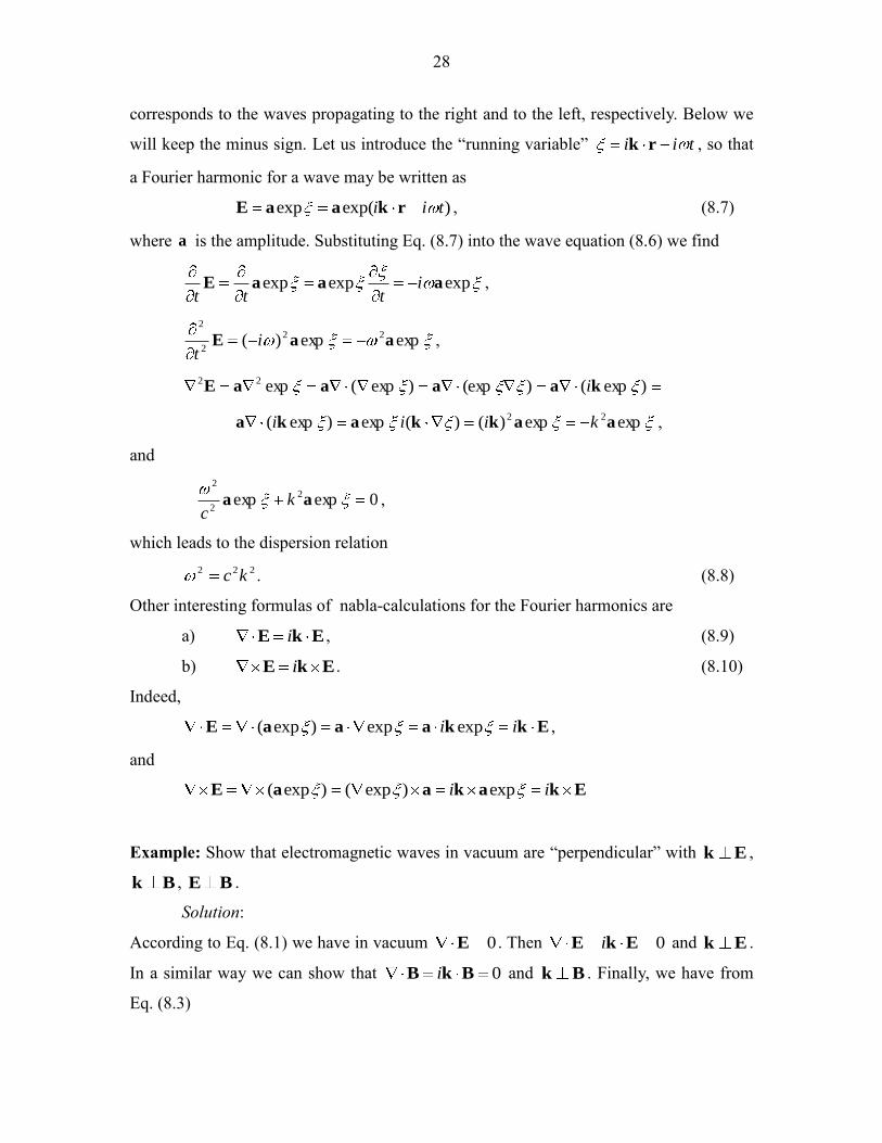
28

corresponds to the waves propagating to the right and to the left, respectively. Below we

will keep the minus sign. Let us introduce the “running variable” tii rk , so that

a Fourier harmonic for a wave may be written as

)exp(exp tii rkaaE , (8.7)

where a is the amplitude. Substituting Eq. (8.7) into the wave equation (8.6) we find

expexpexp aaaE ittt

,

expexp)( 22

2

2

aaE it

,

)exp()(exp)exp(exp22kaaaaE i

expexp)()(exp)exp( 22aakkaka kiii ,

and

0expexp 2

2

2

aa kc

,

which leads to the dispersion relation

222 kc . (8.8)

Other interesting formulas of nabla-calculations for the Fourier harmonics are

a) EkE i , (8.9)

b) EkE i . (8.10)

Indeed,

EkkaaaE ii expexp)exp( ,

and

EkakaaE ii exp)exp()exp(

Example: Show that electromagnetic waves in vacuum are “perpendicular” with Ek ,

Bk , BE .

Solution:

According to Eq. (8.1) we have in vacuum 0E . Then 0EkE i and Ek .

In a similar way we can show that 0BkB i and Bk . Finally, we have from

Eq. (8.3)

29

BEk ii ,

that is

Ek

B .

9. Other integral theorems.

9.1 Hydrostatics.

Derive the differential equation describing pressure distribution for a fluid at rest in a

gravitational field.

Solution:

We consider an arbitrary volume in the fluid similar to that shown in Fig. 4.2. The fluid is

at rest, which means that the fluid velocity is zero 0u and the net force acting on the

fluid inside the volume is zero too. The net force results from the gravity force and the

pressure force, which leads to the equation of force balance

0pressuregravity FF .

The gravity force is calculated according to Eq. (2.5), and the pressure force is

determined by Eq. (5.24), which leads to

0

00 SV

dPdV Sg .

Using the respective integral theorem we reduce the surface integral to the volume

integral

00 VS

dVPdP S

and obtain the integral equation

0)(

0V

dVPg .

Since the equation holds for an arbitrary volume, then we can write it in a differential

form

Pg . (9.1)

30

In the everyday situation we have approximately constant gravity acceleration

);0;0( gg , where we have chosen z-axis pointing upwards. In that case the equation

of hydrostatics takes the form

gz

P, 0

x

P, 0

y

P. (9.2)

In the case of incompressible fluid with const the solution to Eq. (9.2) is

0PgzP . (9.3)

An interesting consequence of the solution Eq. (9.3) is that pressure at the bottom of a

vessel does not depend on the vessel form, but only on the fluid depth. As a result,

pressure at the bottom of the tanks shown in Fig. 9.1 is the same.

Fig. 9.1. Tanks of water with equal pressure at the bottom

9.2 The Archimedes force.

Find the pressure force acting on a body immersed in an incompressible fluid (the

Archimedes force).

Solution:

The pressure force is determined by Eq. (5.24), which may be transformed into the

volume integral

0 0S V

dVPdP SF .

h

31

In that case P stands for virtual pressure distribution, which could take place if the

fluid filled the whole space. The virtual pressure distribution obeys the hydrostatic

equation Eq. (9.1) with standing for the fluid density. On the other hand, it is obvious

that a body at rest does not change the pressure distribution. Then the pressure force

acting on the body is

body

VVV

VdVdVdVP gggF

000

.

Thus, the fluid pressure force on a body is equal to the weight of the fluid, which could

fill the volume of the body. The force is directed upwards.

9.3 Force on a magnetic dipole.

We consider a magnetic dipole, which is, actually, a small loop L of wire with current I ,

with surface area dSd nS ˆ , see Fig. 9.3. The magnetic moment of the dipole is defined

as

Sμ dI ,

The magnetic dipole is placed in a magnetic field )(rB .

Fig. 9.3. Magnetic dipole placed in a magnetic field

Example: Find the force acting on the dipole.

Solution:

We use Ampere’s law Eq. (4.1) for the force acting on an element of the wire

BrF dId .

The total force is

L

dI BrF .

Using the integral theorems we can transform the above formula to

I L

dS B(r)

32

dSIdIdIdSdSL

BnBSBrF )ˆ()( .

Standard -calculations lead to

)ˆ()(ˆ)ˆ()ˆ( BnBnBnBn ,

since 0B . Then

)()ˆ( BμBSBnF dIdSIdS

.