Example 15.8Manufacturing at the Great Threads Company with Fixed Costs

Integer Programming Models

15.1 | 15.2 | 15.3 | 15.4 | 15.5 | 15.6 | 15.7 | 15.9 | 15.10 | 15.11

Objective

To use IP to find the profit-maximizing product mix, using binary variables to deal with the fixed costs.

15.1 | 15.2 | 15.3 | 15.4 | 15.5 | 15.6 | 15.7 | 15.9 | 15.10 | 15.11

Background Information

The Great Threads Company is capable of manufacturing shirts, shorts, and pants.

Each type of clothing requires that Great Threads have the appropriate type of machinery available.

The machinery needed to manufacture each type of clothing must be rented at the following rates: shirt machinery, $2500 per week; shorts machinery, $3200 per week; pants machinery, $3000 per week.

15.1 | 15.2 | 15.3 | 15.4 | 15.5 | 15.6 | 15.7 | 15.9 | 15.10 | 15.11

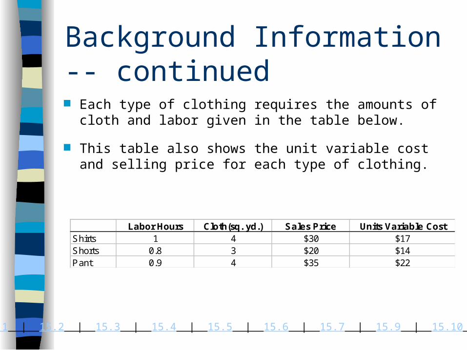
Background Information -- continued Each type of clothing requires the amounts of cloth

and labor given in the table below.

This table also shows the unit variable cost and selling price for each type of clothing.

Labor Hours Cloth(sq. yd.) Sales Price Units Variable CostShirts 1 4 $30 $17Shorts 0.8 3 $20 $14Pant 0.9 4 $35 $22

15.1 | 15.2 | 15.3 | 15.4 | 15.5 | 15.6 | 15.7 | 15.9 | 15.10 | 15.11

Background Information -- continued We first note that the cost of producing x shirts during

a week is 0 if x=0, but it is 2500+17x if x >0.

This cost structure violates the proportionality assumption which is needed for a linear model.

If proportionality were satisfied, then the cost of making, say, 10 shirts would be double the cost of making 5 shirts.

15.1 | 15.2 | 15.3 | 15.4 | 15.5 | 15.6 | 15.7 | 15.9 | 15.10 | 15.11

Background Information -- continued However, because of the fixed cost, the total cost of

making 5 shirts is $2585, and the cost of making 10 shirts is only $2670.

The violation of proportionality requires us to resort to 0-1 variables to obtain a linear model.

15.1 | 15.2 | 15.3 | 15.4 | 15.5 | 15.6 | 15.7 | 15.9 | 15.10 | 15.11

Solution

To model the Great Threads problem, we need to keep track of the following:

– number of shirts, shorts and pants produced

– 0-1 variable for each type of clothing that indicates whether any of that type of clothing is produced

– resource usage of labor and cloth

– total profit, which equals revenue from sales minus the cost of renting machines minus the variable cost of producing clothing.

15.1 | 15.2 | 15.3 | 15.4 | 15.5 | 15.6 | 15.7 | 15.9 | 15.10 | 15.11

THREADS.XLS

This file provides the setup to develop the model seen on the next slide.

15.1 | 15.2 | 15.3 | 15.4 | 15.5 | 15.6 | 15.7 | 15.9 | 15.10 | 15.11

15.1 | 15.2 | 15.3 | 15.4 | 15.5 | 15.6 | 15.7 | 15.9 | 15.10 | 15.11

Developing the Model

The model can be formulated as follows:

– Inputs. Enter the given inputs in the ranges.

– 0-1 values for shirts, short, and pants. Enter any trial values for the 0-1 variables for shirts, shorts, and pants in the ProduceAny range.

– Shirts, shorts and pants produced. Enter any trial values for the number of shirts, shorts and pants produced in the Produced range.

15.1 | 15.2 | 15.3 | 15.4 | 15.5 | 15.6 | 15.7 | 15.9 | 15.10 | 15.11

Developing the Model -- continued

– Labor and cloth used. Calculate the total amount of labor hours used by entering the formula =SUMPRODUCT(Produced,B6:D6) in cell B23. Then copy this to cell B24 to calculate the amount of cloth used.

– Upper limits on production quantities. Now we come to the tricky part of the formulation. We need to ensure that if any of the given type of clothing is produced, then its 0-1 variable equals 1. This ensures that the model incurs that cost of renting a machine for this type of clothing. We could easily implement these with IF statements but Solver is unable to deal with IF statements. Therefore, instead we model the fixed cost constraints as follows Shirts produced <= (Maximum number of shirts that could be produced) * (0-1 variable for shirts).

15.1 | 15.2 | 15.3 | 15.4 | 15.5 | 15.6 | 15.7 | 15.9 | 15.10 | 15.11

Developing the Model -- continued

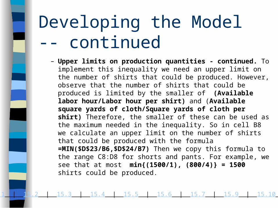
– Upper limits on production quantities - continued. To implement this inequality we need an upper limit on the number of shirts that could be produced. However, observe that the number of shirts that could be produced is limited by the smaller of (Available labor hour/Labor hour per shirt) and (Available square yards of cloth/Square yards of cloth per shirt) Therefore, the smaller of these can be used as the maximum needed in the inequality. So in cell B8 we calculate an upper limit on the number of shirts that could be produced with the formula =MIN($D$23/B6,$D$24/B7) Then we copy this formula to the range C8:D8 for shorts and pants. For example, we see that at most min{(1500/1), (800/4)} = 1500 shirts could be produced.

15.1 | 15.2 | 15.3 | 15.4 | 15.5 | 15.6 | 15.7 | 15.9 | 15.10 | 15.11

Developing the Model -- continued

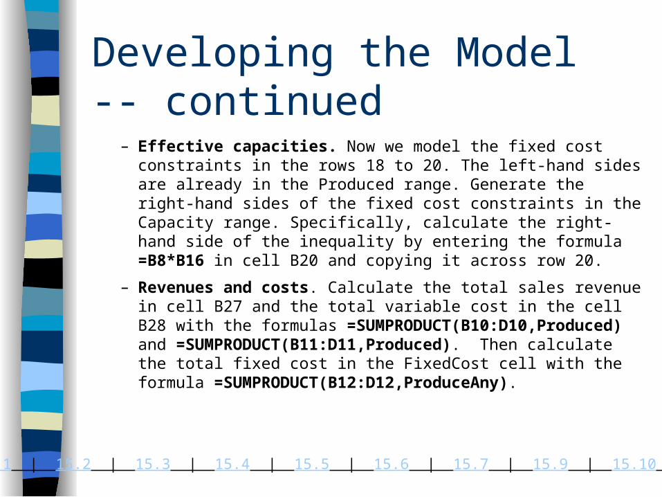
– Effective capacities. Now we model the fixed cost constraints in the rows 18 to 20. The left-hand sides are already in the Produced range. Generate the right-hand sides of the fixed cost constraints in the Capacity range. Specifically, calculate the right-hand side of the inequality by entering the formula =B8*B16 in cell B20 and copying it across row 20.

– Revenues and costs. Calculate the total sales revenue in cell B27 and the total variable cost in the cell B28 with the formulas =SUMPRODUCT(B10:D10,Produced) and =SUMPRODUCT(B11:D11,Produced). Then calculate the total fixed cost in the FixedCost cell with the formula =SUMPRODUCT(B12:D12,ProduceAny).

15.1 | 15.2 | 15.3 | 15.4 | 15.5 | 15.6 | 15.7 | 15.9 | 15.10 | 15.11

Developing the Model -- continued

– Revenues and costs - continued. Note that this formula picks up the fixed costs for only those products with 0-1 variables equal to 1. Finally, calculate the total profit in the Profit cell with the formula =B27-SUM(B28:B29)

15.1 | 15.2 | 15.3 | 15.4 | 15.5 | 15.6 | 15.7 | 15.9 | 15.10 | 15.11

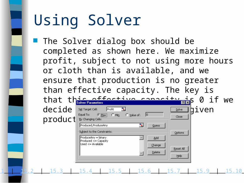
Using Solver The Solver dialog box should be completed as shown

here. We maximize profit, subject to not using more hours or cloth than is available, and we ensure that production is no greater than effective capacity. The key is that this effective capacity is 0 if we decide not produce any of the given product.

15.1 | 15.2 | 15.3 | 15.4 | 15.5 | 15.6 | 15.7 | 15.9 | 15.10 | 15.11

Optimal Solution

From the optimal solution we see that Great Threads should produce 1667 pairs of pants but no shirts or shorts.

The total profit is $18,667.

It might be helpful to think of this solution occurring in two stages:

– In the first stage Solver determines which products to produce.

– In the second stage Solver specifies how many pairs of pants to produce.

15.1 | 15.2 | 15.3 | 15.4 | 15.5 | 15.6 | 15.7 | 15.9 | 15.10 | 15.11

Optimal Solution -- continued The Great Threads management might not be very excited

about being a pants-only shop.

Suppose they wanted to ensure that at least two types of clothing are produced at positive levels.

One approach to do this would be to add another constraint, namely, that the sum of the 0-1 values in row 16 is greater than or equal to 2. When Solver reruns, the 0-1 variable for shirts becomes 1, but no shirts are produced!

To force the company to produce shirts, we would need to add constraints which would cost Great Threads money.