examination of the effects of bottlenecks and …
TRANSCRIPT
EXAMINATION OF THE EFFECTS OF BOTTLENECKS AND PRODUCTIONCONTROL RULES AT ASSEMBLY STATIONS
By
TIMOTHY M. ELFTMAN
A THESIS PRESENTED TO THE GRADUATE SCHOOLOF THE UNIVERSITY OF FLORIDA IN PARTIAL FULFILLMENT
OF THE REQUIREMENTS FOR THE DEGREE OFMASTER OF SCIENCE
UNIVERSITY OF FLORIDA
1999

Copyright 1999
by
Timothy M. Elftman

iii
ACKNOWLEDGMENTS
During the last few years, I have received an incredible amount of opportunities
and was given many chances to broaden my experiences. I do not believe I could
acknowledge everyone who has helped me during this time. But I will highlight specific
people whom I believe deserve more than this simple recognition.
First and foremost, I would like to thank Sam and Charlene Scaggs for their
emotional support over the last few years. I would also like to thank June Cheng for her
support and understanding. I know it has been difficult. Finally, I thank Dr Tufekci for
his insight and support in this paper’s development.
iv
TABLE OF CONTENTS
page
ACKNOWLEDGMENTS .............................................................................................. iii
LIST OF TABLES ......................................................................................................... vi
LIST OF FIGURES....................................................................................................... vii
ACRONYMS ................................................................................................................. ix
ABSTRACT....................................................................................................................x
1 INTRODUCTION........................................................................................................1
1.1 Motivation.................................................................................................................11.2 Fundamentals of Manufacturing Control Systems.......................................................81.3 Manufacturing Systems Philosophies........................................................................111.4 Manufacturing System Control Methodologies.........................................................12
1.4.1 MRP and MRPII Systems ...............................................................................121.4.2 DBR System ...................................................................................................151.4.3 Kanban System................................................................................................161.4.4 CONWIP ........................................................................................................181.4.5 Pull-Push Systems ...........................................................................................191.4.6 Comparison of Production Methodologies.......................................................21
MRP / MRPII and DBR .....................................................................................21MRP / MRPII and Kanban .................................................................................22Kanban and CONWIP ........................................................................................22CONWIP and Push ............................................................................................23JIT and TOC......................................................................................................23
1.4.7 Comparison Summary .....................................................................................241.5 Preliminaries of Queuing Theory..............................................................................241.6 Statistical Hypothesis ...............................................................................................25
2 SIMULATION MODELING AND THE ASSEMBLE SYSTEM MODEL................29
2.1 Simulation Modeling................................................................................................292.1.1 Emulated Flexible Manufacturing Laboratory Software ...................................29
Factory Setup Object..........................................................................................30Machine Object ..................................................................................................31

v
Dispatch and Raw Material Object .....................................................................322.1.2 Comparison of EFML to Traditional Simulation Programs ..............................32
2.2 Simulation Model.....................................................................................................332.2.1 Experimental Conditions .................................................................................362.2.2 Calculations ....................................................................................................37
Cycle Time.........................................................................................................37Final Inventory Status ........................................................................................37
3 FEEDER LINE ANALYSIS.......................................................................................38
3.1 MRP Feeder Lines ...................................................................................................383.2 Kanban Feeder Lines................................................................................................443.3 CONWIP Feeder Line..............................................................................................503.4 Feeder Line Production Control Systems Summary and Conclusions of
Findings ...................................................................................................................55
4 ASSEMBLY SYSTEM ANALYSIS ..........................................................................58
4.1 Pure Push Assembly Systems Using a Synchronization Process ................................604.2 Pure Push Assembly Systems with No Synchronization Process ...............................63
4.2.1 Process Analysis of Unmatched Feeder Line Inventory ....................................684.2.2 Verification of Analysis ...................................................................................69
4.3 Pull-Push Assembly Systems ....................................................................................704.4 Hybrid Pull/Push-Push Assembly Systems ................................................................744.5 Assembly System Summary and Conclusions of Findings .........................................79
5 ASSEMBLY SYSTEM COMPARISON ANALYSIS ................................................82
5.1 Push and Pull-Push Assembly Systems .....................................................................845.2 Push and Hybrid Pull/Push-Push Assembly Systems .................................................855.3 Hybrid and Pull-Push Assembly Systems ..................................................................855.4 Assembly System Comparison Summary of Findings ................................................86
6 CONCLUSIONS........................................................................................................88
GLOSSARY OF TERMS..............................................................................................92
LIST OF REFERENCES...............................................................................................94
BIOGRAPHICAL SKETCH .........................................................................................96

vi
LIST OF TABLES
Table page
1.1: Hypothesis Test on Variance...................................................................................261.2: Hypothesis Test on Means of Large Samples ..........................................................261.3: Hypothesis Test on Means of Small Samples...........................................................274.1: Assembly System Types..........................................................................................594.2: Series Comparison of Actual Feeder Line Inventory to the Predicted Value.............70

vii
LIST OF FIGURES
Figure page
1.1: Generalized Assembly Process ..................................................................................51.2: Synchronization Process ...........................................................................................61.3: General Push System ................................................................................................91.4: General Pull System................................................................................................101.5: MRP Process ..........................................................................................................141.6: Single Card Kanban Process....................................................................................171.7: CONWIP Process ...................................................................................................191.8: Pull – Push Process.................................................................................................202.1: Feeder Line Production Process..............................................................................332.2: Assembly System Production Process.....................................................................342.3: Modified Simulation Model Configuration ..............................................................352.4: EFML Simulation Model ........................................................................................363.1: Analyst Procedure...................................................................................................393.2: Throughput Analysis of 3 Machine MRP Lines– Interarrival Time Constant ............393.3: Throughput Analysis of 3 Machine MRP Lines– Bottleneck Position Constant........403.4: WIP Analysis of 3 Machine MRP Lines – Interarrival Time Constant ......................413.5: WIP Analysis of 3 Machine MRP Lines– Bottleneck Position Constant ...................423.6: Cycle Time Analysis of 3 Machine MRP Lines– Interarrival Time Constant.............433.7: Cycle Time Analysis of 3 Machine MRP Lines– Bottleneck Position Constant ........443.8: Throughput Analysis of 3 Machine Kanban Lines– Card Allocation Constant ..........453.9: Throughput Analysis of 3 Machine Kanban Lines– Bottleneck Position Constant ....463.10: WIP Analysis of 3 Machine Kanban Lines– Card Allocation Constant ...................473.11: WIP Analysis of 3 Machine Kanban Lines– Bottleneck Position Constant .............483.12: Cycle Time Analysis of 3 Machine Kanban Lines– Card Allocation Constant.........493.13: Cycle Time Analysis of 3 Machine Kanban Lines– Bottleneck Position Constant ...503.14: Throughput Analysis of 3 Machine CONWIP Lines– Cards Allocated Constant ....513.15: Throughput Analysis of 3 Machine CONWIP Lines– Bottleneck Position Constant523.16: Cycle Time Analysis of 3 Machine CONWIP Lines– Cards Allocated Constant .....543.17: Cycle Time Analysis of 3 Machine CONWIP Lines– Bottleneck Position Constant554.1: Throughput Analysis of Base Push Assembly System..............................................604.2: WIP Analysis of Base Push Assembly System.........................................................614.3: Cycle Time Analysis of Base Push Assembly System...............................................634.4: Unmatched Inventory after 4000 Batches - Bottleneck Feeder Line.........................654.5: Unmatched Inventory after 4000 Batches - Dual Nonbottleneck Feeder Lines.........654.6: Unmatched Inventory after 4000 Batches - Assembly Systems with One Bottleneck
Feeder Line............................................................................................................66

viii
4.7: Unmatched Inventory after 4000 Batches - Dual Bottleneck Feeder Lines ...............664.8: Unmatched Inventory after 4000 Batches - Nonbottleneck Feeder Line...................674.9: Unmatched Inventory after 4000 Batches - Assembly Systems with Two Bottleneck
Feeder Lines ..........................................................................................................674.10: Assembly Station Raw Material Combination........................................................694.11: Throughput Analysis of Pull-Push Assembly System .............................................714.12: WIP Analysis of Pull-Push Assembly System.........................................................724.13: Cycle Time Analysis of Pull-Push Assembly System..............................................734.14: Throughput Analysis of Hybrid Pull/Push-Push System.........................................754.15: WIP Analysis of Hybrid Pull/Push-Push System ....................................................774.16: Cycle Time Analysis of Hybrid Pull/Push-Push System..........................................785.1: Throughput Comparison Analysis of Assembly Systems..........................................835.2: WIP Comparison Analysis of Assembly Systems .....................................................835.3: Cycle Time Comparison Analysis of Assembly Systems...........................................83

ix
ACRONYMS
This thesis uses a variety of acronyms that the reader may not be aware of or that
differ from literature source to literature source. These acronyms are defined when first
used, but are supplied here to aid the reader.
Acronym DefinitionBOM Bill of MaterialsCONWIP Constant Work in ProcessCT Cycle TimeDBR Drum Buffer RopeEFML Emulated Flexible Manufacturing LaboratoryMPS Master Production ScheduleMRP Material Requirement PlanningMRPII Manufacturing Resource PlanningTOC Theory of ConstraintsTH ThroughputWIP Work in Process

x
Abstract of Thesis Presented to the Graduate Schoolof the University of Florida in Partial Fulfillment of the
Requirements for the Degree of Master of Science
EXAMINATION OF THE EFFECTS OF BOTTLENECKS AND PRODUCTIONCONTROL RULES AT ASSEMBLY STATIONS
By
Timothy M. Elftman
May 1999
Chairman: Dr. Suleyman TufekciMajor Department: Industrial and Systems Engineering
In manufacturing centers products manufactured at different locations are often
joined together at assembly stations. If not managed properly this common event can lead
to orphaned products, lost throughput, and increased WIP. All of which will result in lost
capital for the manufacturing center.
This study analyzes an assembly line, which is fed by three parallel independent
feeder lines, to determine characteristics unique to assembly systems. The assembly
systems are managed by MRP / MRPII, Pull-Push, and Pull/Push-Push Hybrid production
control methods. The study focuses on the effects of bottlenecks, batch synchronization,
and production control methods on the assembly systems’ throughputs, WIPs, and cycle
times.
The study will show that assembly systems have several unique characteristics.
The first characteristic occurs in assembly systems that use push control techniques to

xi
manage the assembly station. In these systems if the bottleneck feeder lines are not
synchronized with the nonbottleneck feeder lines, instability results. This instability is the
accumulation of the nonbottleneck feeder lines’ product at the assembly station. If the
assembly system is left unchanged the orphaned products can grow infinite in number.
The second characteristic occurs in assembly systems with two bottleneck feeder lines. In
these systems the probability of both bottleneck feeder lines finishing a product
simultaneously is zero. The result is a delay in processing at the assembly station that can
decrease the system’s throughput. Although all of the assembly systems with two
bottleneck feeder lines experience this delay only the systems that manage the bottleneck
feeder lines with pull techniques show a significant reduction in throughput. The third
characteristic concerns assembly systems that are controlled entirely by push techniques.
In these systems if the nonbottleneck feeder lines are controlled by pull techniques, the
assembly system will experience decreased WIP with no change in throughput. The fourth
and final characteristic is that assembly systems, which manage the bottleneck feeder lines
with pull techniques, can outperform systems that manage the bottleneck feeder lines with
push techniques.

1
CHAPTER 1
INTRODUCTION
1.1 Motivation
Manufacturing centers are a conglomerate of workstations, assembly stations,
bottleneck stations, dispatch stations, buffers, inventories, forklifts, hand trucks, and
personnel. The center’s dependence on the conglomerate’s performance is similar to a
human’s dependence on his muscles, tissues, eyes, hands, legs, organs, skin, and brain. As
we are more than the sum of our parts so are manufacturing centers.
As succinctly put by Eliyahu Goldratt [7] the primary goal of manufacturing is to
make profit in the present and in the future. Accomplishing this goal has been a daunting
challenge for manufacturing managers since the dawn of time. There are many obstacles
in a manufacturing enterprise that prevents management from accomplishing this goal.
Goldratt calls these obstacles constraints or bottlenecks. The Theory of Constraints
(TOC) is a management philosophy proposed by Goldratt that deals with managing system
constraints or bottlenecks. The five-step methodology focuses on identifying the system
constraints, exploiting the constraint, subordinating the rest of the system to the needs of
the constraint, improving the constraint, and repeating the process continually.
In a factory the bottlenecks are usually those machines or processes which control
the throughput of the system. Managing the bottlenecks effectively and efficiently yields
higher system throughput. Many production control systems have been proposed to

2
improve throughput in the past. Among them are the Materials Requirement Planning
(MRP), Just-in-Time (JIT), Kanban, Constant Work in Process (CONWIP), and Drum-
Buffer-Rope (DBR) systems. In this thesis an analysis of bottlenecks and their impact on
throughput, work-in-process (WIP), and cycle time in manufacturing systems where three
parallel production lines feed components into an assembly line is carried out.
Successful manufacturing centers are required to identify and manage their
system’s throughput, WIP, and cycle time. Here, throughput is the number of final
products produced per unit time by the system, WIP is the material within the system
undergoing transformation into a final product, and cycle time is the average amount of
time required for raw material to be transformed into a final product. Insufficient
throughput leads to unmet demand. Excessive WIP requires tying up excessive capital.
Excessive cycle time leads to the loss of customer orders. In short, if any of these
parameters are not managed properly, then the manufacturing center loses money. These
parameters are influenced by process variability, process time, process reliability, system
bottlenecks, and the production control system used.
Recent work has investigated how bottlenecks affect a system’s throughput, WIP,
and cycle time in relation to different control methodologies. The goal of these works is
to determine optimal settings of control parameters within the production control systems,
and selecting the appropriate production control systems for different manufacturing
environments. The current manufacturing control systems may be classified into three
categories. The first is MRP and its successor Manufacturing Resource Planning
(MRPII). These control systems push materials into the production facility based on
forecasted demand, and are thus known as push systems. In the second category of

3
control systems, known as pull systems, the material is released into the production facility
only when the demand for the end product triggers it. Since the material is released into
the system only when it is needed, these control system are also called JIT systems. The
two popular implementations of JIT control systems are Kanban (card) control systems
and CONWIP control systems. In all JIT systems the WIP is controlled by the number of
authorization cards assigned to the individual workstations or system of stations. The
third category of control systems is mixed control systems. In these systems, the pull and
push control systems are used to manage certain segments of the production line.
Examples of mixed control systems are DBR, pull-push and push-pull control systems.
These systems will be further defined later in this section.
There is a great amount of literature evaluating the performance of these systems.
Cook demonstrates that serial production systems using DBR results in greater average
throughput and lower levels of WIP variance than when the same system is managed by
kanban [4]. Guide in the analysis of a re-manufacturing facility proves that DBR results in
a reduction in WIP and throughput variance compared to MRP [8]. Bonvik et al. in the
analysis of CONWIP, kanban, and pull-push production control systems demonstrates that
the pull-push systems carries the lowest WIP at any particular throughput level with the
kanban system generally carrying the highest WIP [3]. Altug also demonstrates the
superiority of the pull-push control system over pure MRP, kanban, and CONWIP [1].
The above analyses were mainly conducted with serial systems, or flow lines, as the case
of most manufacturing studies, but serial systems only represent a portion of production
systems in manufacturing.

4
The main work done with assembly systems (systems containing parallel
production lines feeding an assembly line) is modeled as a fork-join with blocking type of
queuing system. The fork operation is when a product is decomposed into smaller units
with each unit following a separate production process. The join operation, which occurs
at the assembly station, is the synchronization of operations over a set of units. In other
words, multiple parallel production lines or workstations feed an assembly station different
components. The assembly station then joins the components. Blocking is the limiting
factor of the number of units in the model. All fork-join articles provide description of
how mathematical modeling techniques can be applied to manufacturing control
methodologies, and assembly systems. Yves Dallery et al. derived methods of modeling
kanban and assembly operations in production facilities [5]. Rao et al. reviews the use of
queuing theory in flexible manufacturing systems, computer-integrated manufacturing, and
kanban systems [13]. Agnetis et al. studies the effects that push, pull, and synchronization
procedures have on assembly stations by using simulation [2]. His results indicate that
push systems lead to increased WIP compared to pull. Furthermore, the results show that
pull systems have increased throughput compared to synchronized push systems.
The assembly system of Agnetis’ study consists of a main production line with
assembly stations located within it. The assembly stations are fed from the main line and
other feeder lines. In the assembly system it is detrimental for the main line to be balked.
By balking the main line the throughput of the system is reduced. If the feeder line’s
product is late in arriving to the assembly station, or tardy, the productivity suffers.
Therefore Agnetis’ study used the system’s throughput and WIP as well as the number of
tardy jobs as performance indicators.

5
In this study the performance indicators are system throughput, cycle time, and
WIP. The assembly system, as indicated in figure 1.1, will be studied to determine general
characteristics of the push, pull, and synchronization strategies at the assembly station.
Figure 1.1: Generalized Assembly Process
In literature, assembly stations are stations where the act of joining components is
carried out. The components to be joined are not necessarily produced in that production
system. By evaluating a process where the synchronization of sub-components is of
valued importance the use of the assembly station term holds special significance. The
assembly station is the station which two or more workstations feed with different
products. The assembly station combines these items into its own unique product. A
workstation is a station that does not combine products from two or more workstations.
A workstation has one input and one output per product type. A sequential series of
workstations is referred to as a serial production line or flow line. Parallel production
lines feeding an assembly station are feeder lines. An assembly station followed by a
Line 4 Machine 10 Machine 12Machine 11
Line 3 Machine 7 Machine 9Machine 8
Line 2 Machine 4 Machine 6Machine 5
Line 1 Machine 1 Machine 3Machine 2

6
sequential series of workstations is an assembly line. A system of two or more production
lines feeding an assembly line is an assembly system. The feeder lines that have the lowest
average throughput are the bottleneck feeder lines, and the other feeder lines are the
nonbottleneck feeder lines.
Figure 1.2: Synchronization Process
A synchronization process occurs when each of the components used in the
assembly station’s product is introduced into the assembly system simultaneously to
specifically combine with one another. For example the product C1, in figure 1.2, is
manufactured from items that were introduced to the assembly system simultaneously. If
product A1 is present at the assembly station and product B1 is not present, then A1 is
regarded as unmatched. A consequence of this synchronization process is that the
maximum amount of unmatched product A1 waiting at the assembly station is the total
sum of unprocessed and processing B0 items.
The primary purpose of this work is to study the effects of bottlenecks on an
assembly system under different production rules. In particular the location of the
A0 is transformed to A1
A1 and B1 are combined into C1
Raw Material A0
Raw Material B0
B0 is transformed to B1

7
bottlenecks relative to the assembly station and the resulting effects on selected
performance indicators of throughput, WIP, and cycle time will be studied. The goal of
this thesis will be achieved in the following manner.
1. Decompose the manufacturing system into its component production lines.
2. Analyze these subsystems with one and two bottlenecks at differing locations,
following differing production rules, and using differing control parameters.
3. Use the information generated in Step 2, to design a push system with a
synchronization procedure, a push system without a synchronization
procedure, a pull-push system, and a hybrid pull/push-push system.
4. Analyze these systems with two bottlenecks in a single feeder line.
5. Analyze these systems with one bottleneck in a feeder line, and one bottleneck
in the assembly line.
6. Analyze these systems with the bottlenecks in two separate feeder lines.
7. Compare all control systems in regard to throughput, WIP, and cycle time.
All statistical analyses will be conducted using hypothesis tests at an α level of
0.05. The throughputs and the WIPs will be compared by using t-statistics, and the cycle
times will be compared using by z-statistics to determine the relation the parameters have
to one another. The experimental data samples were generated from the following two
simulation software programs: Emulated Flexible Manufacturing Laboratory (EFML), and
Arena.
The remainder of the paper is organized in the following manner. The latter part
of this chapter will provide background information in regard to manufacturing control

8
systems, statistical hypothesis testing, and queuing theory. Chapter 2 provides
information on the EFML software and the simulation model. Chapter 3 is the in-depth
analysis of the feeder lines under MRP, kanban, and CONWIP production rules. Chapter
4 is the in-depth analysis of the four assembly system types. Chapter 5 is the comparison
of the assembly systems. Chapter 6 is the summary of the results and recommendations.
1.2 Fundamentals of Manufacturing Control Systems
There are two primary manufacturing control systems: push and pull. All other
control systems are either combinations or derivatives of these two systems. This section
will describe the theories and philosophies associated with manufacturing production
control and the following sections will be used to define different techniques that have
been developed to implement these philosophies.
Many theories have been proposed in managing manufacturing. In a flow shop
environment each product follows a fixed routing. In a job shop environment the routing
depends on the shop and the job being processed. At each station, buffers or finite storage
spaces exist for receiving incoming material and storing completed units. The buffers act
as a safety net to guard against line starvation and blockage caused by random events.
Manufacturing control systems manage how products are passed on, how buffers are
utilized, and when raw material enters the system.
“Push” control systems utilize forecasted demand to determine a production
schedule. The production schedule sets when raw material is delivered to the appropriate
workstations. Each workstation provides the necessary processing to the units waiting in
its buffer prior to releasing it to be transferred to the next downstream station. This cycle

9
of receiving, processing and releasing of material is carried out until the end product is
complete. In a push control system shipping of goods downstream is independent of the
downstream stations’ condition. This independence can cause problems if the downstream
station is offline. If the downstream station is offline, the WIP in the system escalates until
the station is online again. The WIP may or may not decrease at this time.
A push system is represented in figure 1.3. The arrows in the diagram refer to the
movement of the product through the system. Since the production schedule represents
demand information, the quantity of moving products represents the movement of
information in the system.
Figure 1.3: General Push System
“Pull” systems rely on the status of the system to determine production. In this
type of system, inventory is controlled through a system of cards. The number of cards
available determines the maximum allowable inventory for a particular workstation or
system of workstations. In such a system the production rate is determined by how the
finished goods of the final workstation is demanded by the customer. When the finished
goods are removed from the system the cards associated with these units are released.
Process 1 Process 3 Process 4Process 2
Raw Material
End Product

10
The released cards enable the final station to procure additional material from the
upstream station to process. Upon procurement of raw material from the upstream station
and release of the associated cards, the upstream station is able to obtain its own raw
material from its upstream station. This process of card release and material procurement
is repeated throughout the system until the raw material of the first station is obtained.
Since product movement is dependent on the condition of the next station, the entire
production line may stop due to the breakdown of an upstream station.
A pull system is represented in figure 1.4. The solid and dashed arrows in the
diagram respectively refer to the movement of the products and information. Since the
cards represent demand information, the movement of cards represents the movement of
information in the system. Unlike the push system, demand information originates in the
final station and proceeds to the initial station.
Figure 1.4: General Pull System
Process 1 Process 3 Process 4Process 2
Raw Material
End Product
The solid line is product being pulled to the next station.The dashed line is the release of cards or informationtransfer.

11
MRP and its successor MRPII are push systems; kanban and CONWIP are pull
systems. Pull systems follow the Just-In-Time (JIT) philosophy, and DBR and some pull-
push systems follow the Theory of Constraints (TOC) philosophy.
1.3 Manufacturing Systems Philosophies
Philosophies in manufacturing systems define goals to be accomplished by control
techniques. The JIT philosophy’s goal is to have raw material of a process delivered just-
in-time for processing. The TOC philosophy’s goal is to maximize profit. Both of these
philosophies ascribe to process improvement. The improvement reduces variabili ty caused
by breakdowns and raw material shortages.
JIT focuses on minimizing the waste in a system by striving for no buffers, no
defects, and no variation. This is accomplished by:
• designing products for optimal quality, cost, and manufacturing ease,
• minimizing the amount of resources used to design and produce the product,
• designing the product to meet the customer’s needs,
• obtaining and maintaining good relationships with suppliers and vendors,
• and, developing a commitment to improving the manufacturing system [12].
When JIT is implemented, its purpose is to set a production rhythm that exploits
the available capacity of the system to fully meet the customer’s demand. Since JIT is a
pull-oriented system, the demand of the customer directly sets the production rhythm.
TOC focuses on maximizing profit now and in the future by maximizing the flow in
a system. This is accomplished by:

12
• identifying the bottleneck in the system,
• scheduling jobs and operations to ensure the complete utilization of the
bottleneck,
• determining the appropriate bottleneck buffer size to guard against upstream
station variability,
• improving bottleneck performance,
• and, then repeating the process [7, 8].
TOC is a profit oriented manufacturing control system. When using the TOC
system throughput is defined as the rate at which money is generate from sales, and
inventory is defined as the amount of money captured in the system [7]. By defining
manufacturing in this manner a bottleneck may be located off the production floor, such as
poor product sales. When TOC is implemented, its purpose is to set a production rhythm
that exploits the bottleneck of the system. The bottleneck is the constraint that hinders
greater throughput. By scheduling the bottleneck of the system, the WIP is reduced while
maintaining high throughput. Since the bottleneck determines the capacity of the system
by improving bottleneck performance, the system’s capacity is improved. [7, 8]
1.4 Manufacturing System Control Methodologies
1.4.1 MRP and MRPII Systems
MRP is the oldest push-type manufacturing control system. Its major components
are the bill of materials (BOM), the master production schedule (MPS), and the materials
requirement planning system. The BOM is a chart that shows the required components at

13
each stage of production starting from the final product, preceding with the intermediate
products, and then ending with the raw material for the initial processes. Each stage of
the BOM lists the quantities and the types of components required in producing that
stage’s product. The MPS contains information such as the time required at each stage of
production, the outstanding order status, the inventory status, and the demand for the final
product. The production time at each stage is regarded as fixed and the demand is
forecasted. The MRP system, as shown below, determines the production schedule.
1. Determine net requirements by subtracting on-hand inventory and scheduled
receipts from demanded requirements.
2. Determine the job lot sizes.
3. Offset the due dates of the individual jobs with the production times of the
product to arrive at the start times.
4. Using the start times, the lot sizes, and the BOM determine the demanded
requirements for the material used in the production of that stages’ product.
5. Starting with the final product repeat this process until all production stages
have been processed.
MRPII adds capacity analysis to MRP by incorporating information such as setup
time, resource requirements, and labor requirements into the MRP system. Through the
use of this information the MRP system provides a more realistic production schedule.
Figure 1.5 demonstrates how the MRP system generates planned order releases or a
production schedule for the manufacturing facility.

14
Figure 1.5: MRP Process
Although extensively used in the United States, MRP and its successor MRPII
have many shortcomings. Some of them are listed below.
• The MRP / MRPII systems do not consider fluctuations in production time due
to worker illness, machine breakdown, demand change, and availability of raw
material. To accommodate for these uncertainties safety stocks and safety lead
times are often used, but the inclusion of the safety stocks and safety lead times
increases inventory levels and production cycle times.
• MRP systems assume fixed cycle times or lead times regardless of the
inventory level. A consequence of this assumption coupled with a large WIP
leads to a large throughput. Regretfully throughput is limited by the
production rate of the bottleneck station. Once the throughput is maximized,
any additional inventory in the system results only in increased cycle time [14].
MPS
Production SchedulePurchase Orders
InventoryBOM
MRP ProcessNet RequirementsJob Lot SizesOffsettingExplosion

15
• The purpose of MRP systems is to meet the projected demand as provided by
the MPS. No effort is specifically expended to improve production.
1.4.2 DBR System
DBR is a newer system of production control that follows the TOC philosophy. In
doing so, it concentrates on managing the flow of products to meet the bottleneck
constraint’s needs. Since the bottleneck acts as a valve controlli ng the system’s
throughput, managing the bottleneck’s throughput manages the system’s throughput. To
maximize the system’s throughput, the bottleneck must utili ze all of its available capacity.
Similar to the MRP / MRPII systems, the DBR system uses a scheduled release of
products to control the production rate, and a safety stock or buffer at the bottleneck to
guard against stoppages from the upstream workstations [8].
Although the DBR control system provides improvement over the MRP / MRPII
systems, it is not immune from shortcomings. Some of them are listed below.
• Failure to locate the bottleneck of the system will result in lost throughput, or
increased WIP and cycle time depending on the false bottlenecks’ location
relative to the real bottleneck.
• The use of fixed lead times to schedule the bottleneck can lead to increased
WIP much as in MRP / MRPII systems.
• Incorrect bottleneck buffer size can result in bottleneck starvation; thus system
throughput is lost [15].

16
1.4.3 Kanban System
The kanban system was developed by Japanese manufacturers to implement the
JIT philosophy. In this system the kanban acts as an inventory control mechanism and
information relay device. It controls the inventory by requiring every batch in production
to be assigned to a kanban. The number of kanbans in the system thus determines the
maximum inventory possible. The kanbans transmit demand information from the
downstream stations to the upstream stations through the number of kanbans available and
how often the kanbans become available.
The single card kanban system, figure 1.6, allocates a set amount of kanban cards
to each workstation in the system. A kanban card is initially attached to a batch to be
processed by that workstation. The kanban card stays attached to the batch until a
downstream workstation has a kanban card available. When this occurs the attached
kanban card is freed from the workstation’s product and the previously freed kanban card
from the upstream workstation becomes assigned to that batch. Thus a free kanban card
allows a workstation to obtain material from the previous station when the material is
available [14].

17
Figure 1.6: Single Card Kanban Process
Successful implementation of the kanban system requires large production runs,
minimal defects, steady demand, reliable workstations, few product types, and reliable
vendors. Determining the number of kanban cards to allocate to each workstation is of
significant importance. One manner of determining the initial amount of kanban cards
uses the formulation below.
N > D * L (1 + α) / a
Here, N equals the number of kanban cards allocated to the workstation, D is the
demanded throughput, L is the cycle time, α is the safety factor, and “a” is the batch size.
N is first estimated by choosing a high α value in the range [0, 1]. Once the number of
kanban cards is determined the system is operated for a set length of time. Depending on
the production system dynamics, N is then adjusted on each separate workstation in an
effort to reduce WIP but maintain throughput [3].
Process 1 Process 3 Process 4Process 2
Raw Material
End Product
The solid line is product being pulled to the next station.The dashed line is the release of cards or information transfer.
18
For all of kanban’s improvements to the production system, it also has its
shortcomings. Some of them are listed below.
• Kanban systems are not suited for manufacturing environments with short
production runs, highly variable product demand, poor quality products, and a
multitude of product types [11].
• A breakdown in the kanban system can result in the entire line shutting down.
• The throughput of a kanban system is not managed but is instead a result of
controlled WIP and known cycle times.
1.4.4 CONWIP
The CONWIP system is a generalized form of the kanban system. Like kanban,
CONWIP uses cards to limit the WIP of a system; unlike kanban the cards are allocated to
a system of workstations instead of just one. This difference allows CONWIP to be
applied in production environments that are detrimental to the kanban system [10].
In a CONWIP system the cards get attached to batches only at the first station.
The card remains affixed to the batch until the batch has finished processing on the final
workstation of the CONWIP system and the batch is used to satisfy a customer’s demand.
The released card is then returned to the initial workstation of the CONWIP line and to
authorize the entry of a new batch into the system.
Under a CONWIP system enough cards should be allocated to ensure the
bottleneck is fully utili zed. If the number of cards is insufficient the bottleneck starves and
thereby reduces the system’s throughput. Figure 1.7 shows the CONWIP process.

19
Figure 1.7: CONWIP Process
Even though CONWIP generally provides improvement over kanban and MRP /
MRPII, it does have its share of shortcomings. Some of them are listed below.
• Kanban systems can achieve higher throughput with lower WIP in some
situations over CONWIP systems.
• CONWIP systems cannot be successfully implemented in a job shop
environment.
• Incorrect card determination can lead to increased WIP or lost throughput for
the system.
• Machine breakdown can bring the entire CONWIP system to a halt.
1.4.5 Pull-Push Systems
Spearman et al. proposed a generalization of DBR that is modeled by using
CONWIP and a push system on a flow line [14]. By using a CONWIP system that
encapsulates all stations between and including the initial and the bottleneck stations, and
using a push system following the bottleneck station, the DBR system is approximated.
Process 1 Process 3 Process 4Process 2
Raw Material
End Product
The solid line is product being pushed to the next station.The dashed line is the release of cards or information transfer.The double line is product being pulled into the system.

20
The DBR system determines a production schedule to ensure bottleneck of the system is
completely utilized. In the DBR system, the bottleneck is protected against variation from
the upstream stations via a buffer prior to the bottleneck. In the pull-push system enough
cards are allocated to the CONWIP segment to ensure the bottleneck is completely
utilized. Prior to the bottleneck a buffer will naturally develop and will be limited in
quantity by the CONWIP cards. Following the bottleneck in both systems the batches are
pushed through as fast as possible. The pull-push process is represented in figure 1.8,
where process 4 is the bottleneck process.
Figure 1.8: Pull – Push Process
Process 1 Process 3 Process 4Process 2
Raw Material
End Product
Process 8 Process 6 Process 5Process 7
The solid line is product being pushed to the next station.The dashed line is the release of cards or information transfer.The double line is product being pulled into the system.Process 4 is the bottleneck.

21
Although the pull-push system provides improvements to pull systems and DBR it
still has some shortcomings. Some of them are listed below.
• Failure to locate the bottleneck of the system will result in lost throughput, or
increased WIP and cycle time depending on the false bottlenecks’ location
relative to the real bottleneck.
• Incorrect card determination can lead to increased WIP or lost throughput for
the system.
• Machine breakdown can bring the entire pull-push system to a halt.
• Increased complexity over pure systems.
1.4.6 Comparison of Production Methodologies
There is extensive literature proving that pull systems tend to have lower WIP and
cycle time mean and variance compared to push systems. Pull systems are also easy to
control since WIP can be controlled directly whereas push systems manage throughput.
On the other hand, push systems can be implemented in many environments [4, 9, 14].
MRP / MRPII and DBR
MRP / MRPII and DBR are very similar systems, the diff erence lies in the focus of
production and the manner in which it is carried out. MRP / MRPII focuses on
maximizing the capacity of the production system. DBR focuses on maximizing the flow
of the production system. As a result DBR experiences reduced WIP levels and are more
capable of adjusting to fluctuations in the production environment [4].

22
MRP / MRPII and Kanban
MRP / MRPII and kanban systems differ in philosophies, environmental settings,
and control methods. MRP / MRPII systems operate under the philosophy of maximizing
throughput, can be applied in most manufacturing environments, and place production
control in the production schedule. Kanban systems use a philosophy of improvement,
require stable environments with large production runs, small setup times, minimal defects,
consistent demand, and places production control on the factory floor. Once the
production environment is achieved, the kanban system can achieve high throughput with
lower amounts of WIP compared to the MRP / MRPII systems [4, 11].
Kanban and CONWIP
Kanban and CONWIP systems only differ in that kanban fixes the inventory on a
per station basis, whereas CONWIP fixes the inventory on a per system basis. This
difference in implementation results in the following performance differences [9, 14].
• CONWIP can be implemented in production environments that have variable
demand and have a multitude of products, whereas kanban requires stable
environments and few product types.
• CONWIP does not attempt to control the location of the WIP in the
production system.
• CONWIP generally results in lower WIP levels than kanban given the same
throughput levels. Kanban in some situations can outperform CONWIP by
optimally placing cards in some systems [6].

23
CONWIP and Push
CONWIP is superior to push systems when the production systems run under the
highest possible throughput rate. In this situation at equivalent throughput rates, the push
system experience higher WIP and cycle time compared to the CONWIP system
[4, 9, 14].
JIT and TOC
TOC and JIT, through different approaches in managing a production
environment, achieve similar results.
• Both systems strive to improve and reduce variation in the production system.
TOC concentrates on improving the bottleneck station, and JIT improves each
station in the system.
• Both systems experience a reduction in WIP compared to MRP / MRPII
systems at equivalent throughputs. TOC accomplishes this by scheduling the
bottleneck to its fullest, and JIT does this by allocating kanban cards to keep
the bottleneck working.
• These systems differ in that TOC generally provides better throughput than JIT
with only slightly higher levels of WIP and greater cycle time [4].

24
1.4.7 Comparison Summary
From the previous descriptions of the above production systems the following can
be inferred.
• Scheduled releases of raw material can lead to increased system WIP,
depending on the variability of the system.
• Complete utilization of bottleneck maximizes system throughput.
• If the system conditions determine the release of raw material, the WIP of the
system is controlled.
• Pull systems are much more susceptible to system variation than push systems.
• Improving the production system can decrease system variability.
1.5 Preliminaries of Queuing Theory
Queuing theory studies how people, messages, and items flow through a system.
Practically all models and formulas developed in queuing theory are for systems in steady
state or equilibrium conditions. For a queuing system to be in steady-state the average
capacity of the system (C) must always be greater than the average arrival of entities to
the system (R). The above statement, C > R, is true for a single server system as well as
for networks of queues, as captured by Little’s Law.
In a steady state queuing system the following fundamental relationship N = λT
always holds true.
Little’s Law states that the average number of customers in a queuingsystem (N) is equal to the average arrival rate of customers to that system(λ), times the average time spent in that system (T). Furthermore, it does

25
not depend upon any specific assumptions regarding the arrival rate or theservice time distribution; nor does it depend on the particular queuingdiscipline within the system. [10, page 17]
In manufacturing, production lines can be viewed as queuing networks. Ergo, the
above law may be adapted as follows: Work-In-Process (WIP) is equal to throughput
(TH) times cycle time (CT).
WIP = TH* CT
1.6 Statistical Hypothesis
A statistical hypothesis is a formal statement concerning the parameters of a
probabili stic distribution. In order to check a parameter’s relationship to a specific value
hypothesis testing procedures are used. In testing a hypothesis a random sample is
obtained from the population under study and used to generate a test statistic. The value
of the test statistic determines whether to reject or fail to reject the null hypothesis, Ho.
The results obtained from the simulation programs often yielded similar results. In
order to test if a difference existed or if one parameter was greater than the other
statistical hypothesis tests were used. Based on the number of runs carried out, different
test statistics were used to validate the null hypothesis. The test results are available in
chapters 3, 4, and 5. Tables 1.1, 1.2, and 1.3 illustrate the types of tests used in the
analysis of the simulation results.

26
Table 1.1: Hypothesis Test on Variance
Hypothesis Test Statistic Criteria for Rejection
Table 1.2: Hypothesis Test on Means of Large Samples
Hypothesis Test Statistic Criteria for Rejection
22
210 : σσ =H
22
211 : σσ ≠H
22
21
0S
SF =
1,1, 212
0 −−> nnFF α
1,1, 21210 −−<
−nnFF α
22
21
0S
SF = 1,1, 210 −−> nnFF α
22
210 : σσ =H
22
211 : σσ >H
22
210 : σσ =H
22
211 : σσ <H
1,1, 1210 −−< − nnFF α22
21
0S
SF =
210 : µµ =H
211 : µµ >H2
22
1
21
210
n
S
n
S
xxZ
+
−=
αZZ >0
210 : µµ =H
211 : µµ ≠H2
22
1
21
210
n
S
n
S
xxZ
+
−=
20 αZZ >
210 : µµ =H
211 : µµ <H2
22
1
21
210
n
S
n
S
xxZ
+
−=
αZZ −<0

27
Table 1.3: Hypothesis Test on Means of Small Samples
Hypothesis Test Statistic Criteria for Rejection
The use of hypothesis tests requires a certain degree of normality for the sample
data. The central limit theorem (CLT) ensures this for the larger samples. The CLT
implies that the sum of n independently distributed random variables regardless of
2
*)1(*)1(
21
222
2112
−+−+−
=nn
SnSnS p
221 −+= nnv
22
21 σσ =
21
210
11
nnS
xxt
p +
−=
210 : µµ =H
211 : µµ ≠Hv
tt,2
0 α>
210 : µµ =H
211 : µµ <Hvtt ,0 α−<
210 : µµ =H
211 : µµ >Hvtt ,0 α>
2
11 2
2
2
22
1
2
1
21
2
2
22
1
21
−
+
++
+
=
n
n
S
n
n
S
n
S
n
S
v
22
21 σσ ≠
2
22
1
21
210
n
S
n
S
xxt
+
−=
210 : µµ =H
211 : µµ ≠Hv
tt,2
0 α>
210 : µµ =H
211 : µµ <Hvtt ,0 α−<
210 : µµ =H
211 : µµ >Hvtt ,0 α>

28
distribution followed is approximately normal. For the smaller samples normality is
assumed.

29
CHAPTER 2
SIMULATION MODELING AND THE ASSEMBLE SYSTEM MODEL
2.1 Simulation Modeling
Simulation is a tool that allows actual or hypothetical facilities or processes to be
studied. Similar to other methods of analysis an accurate model is essential for the
analysis to be meaningful. The simulation models’ advantage over mathematical models is
that it can be used to study large and complex systems quickly. The simulation program’s
speed and its ability to collect system data enables the analyst to study alterations to the
system easily. But unlike mathematical models, simulation cannot place theoretical limits
on a system and it cannot prove innate characteristics of the system.
2.1.1 Emulated Flexible Manufacturing Laboratory Software
The Emulated Flexible Manufacturing Laboratory (EFML) Software is a real-time
simulation program developed in the Industrial and Systems Engineering Department at
the University of Florida. It has been designed using Borland’s Delphi 4.0 and runs on
the Windows NT, 95, and 98 platforms with TCP/IP network communication protocol.
The software creates an interactive environment that allows users to experience the basics
in operation management, and production control systems.
30
EFML is written in an object oriented programming language. Each object in
EFML emulates an actual object in a manufacturing plant and is represented in an object
window. The main objects are factory setup, machine, dispatch and raw material,
transport, repair, and finished goods. These objects communicate with each other using a
message passing protocol over the internet thus allowing large facility and supply chain
management emulation. A small percentage of the software’s capabilities were utilized
during this study. Of all the available objects only the factory setup, machine, and the
dispatch and raw material objects were used.
Factory Setup Object
The factory setup object is the main object of EFML. It controls the factory setup,
the emulation model loading, the starting and stopping of the emulation, and the gathering
of the emulation statistics into a usable report. Additionally this window allows the user
to view and adjust remote system components and parameters.
Once EFML is started, a preset factory can be loaded by selecting “Autoload”
from the “Global” menu, or a factory can be built with the objects available to the user. If
a preset factory is loaded, selecting objects and changing their parameters can alter the
factory. If the user desires to save this change for future factory runs, it can be
accomplished using the “Save” option from the “File” menu.
When the setup is accomplished manually, the user chooses the needed objects
from the “Components” bar and places them in the active setup window. The setup
window serves as a background and moderator for the other objects (windows). The
overall control of the emulation resides in the setup object. In this object, the user adjusts

31
the speed of the emulation, the stop condition, where the report file is saved, and can
manually start and stop the emulation.
Machine Object
The machine object serves a dual purpose. It can be used to represent a process
center or it can emulate an assembly station. During emulation each machine is in one of
four states: idle, running, setup, and breakdown. In the running mode the machine follows
MRP, CONWIP, or kanban production rules. Each of these states and modes of the
machine object are color coded for ease of viewing. The color codes and states are listed
below.
• Idle status and any production process is white.
• Running status and MRP is blue.
• Running status and CONWIP is green.
• Running status and kanban is red.
• Setup status and setup is the color of the production process (green, blue, or
red).
• Breakdown status and any production process is yellow.
When setting up a machine object, the user is asked to specify the incoming and
outgoing batch names and sizes, the production rule to follow, the process distribution and
parameters, as well as the failure rate of the machine. While running, the machine objects
compute the statistics on the mean and variance of the machine’s processing time, the
mean and variance of the machine’s cycle time, the machine’s throughput, the batch’s start
and end times, and the number of batches processed.

32
Batches move through the system as directed by the machine and dispatch objects
and follow the implemented production control system. While at a machine the batch is in
one of three states: waiting in the in-queue buffer, being processed, or waiting in the out-
queue buffer. Following processing the batches are transported to the next machine object
or to the finished goods object.
Dispatch and Raw Material Object
The functions of the dispatch and raw material object include the storage of the
generated BOM, storage of the product routing, managing raw material inventory, and
dispatching of inventory to the appropriate workstations. The dispatching can either be
performed automatically or manually. In addition this object may be used to track
inventory cost and record transaction data.
2.1.2 Comparison of EFML to Traditional Simulation Programs
In traditional simulation programs, model events are determined to occur at a
specific time. The simulation program finds the earliest occurring event, sets its simulation
clock to that time, carries out any required functions, and then looks for the next event to
repeat this process. EFML, unlike the traditional simulation programs, advances through
time and at each clock tick determines if an event has occurred. If an event occurred,
EFML carries out any required functions before advancing to the next clock tick to repeat
the process. In this manner EFML runs in real time and allows individuals to see virtual
processes being accomplished.

33
2.2 Simulation Model
The primary system under analysis is an assembly system composed of three feeder
lines, and a three-station assembly line. The three-workstation feeder lines’ products are
the raw material for the assembly line. The assembly system is depicted in figure 2.1.
Using throughput, WIP, and cycle time as performance indicators, the goal of this
study is to ascertain general effects of push systems with and without batch
synchronization procedures implemented, pull-push systems, and hybrid pull/push-push
systems, in the presence of bottlenecks. In particular the location of the bottlenecks
relative the assembly station and the resulting effects on the performance indicators of the
assembly systems will be studied. The feeder lines, figure 2.4, were studied using one and
two bottlenecks under differing bottleneck locations, differing production rules, and
differing control settings. Following the feeder line study the full assembly system is
studied extensively. In all our experiments the processing times are assumed to be
independently and identically distributed random variables.
Figure 2.1: Feeder Line Production Process
Single LineMachine 1 Machine 3Machine 2

34
The assembly system in this study is assumed to contain two separate bottlenecks
with at least one of the bottlenecks located prior to the assembly station. A description of
the four assembly systems follows. The base push system is a pure push system using a
batch synchronization procedure. Batch synchronization is accomplished by releasing the
raw material to all the feeder lines simultaneously. The pure push systems without a batch
synchronization procedure use different interarrival times for the raw material of the
bottleneck and nonbottleneck feeder lines. The pull-push system uses CONWIP control
rules to manage all of the feeder lines. The assembly line is managed by a push system.
The hybrid pull/push-push system uses a pull process to manage the nonbottleneck feeder
lines and a push process elsewhere. The entire manufacturing assembly system studied in
this paper is shown in figure 2.2.
Figure 2.2: Assembly System Production Process
Line 4 Machine 10 Machine 12Machine 11
Line 3 Machine 7 Machine 9Machine 8
Line 2 Machine 4 Machine 6Machine 5
Line 1 Machine 1 Machine 3Machine 2
35
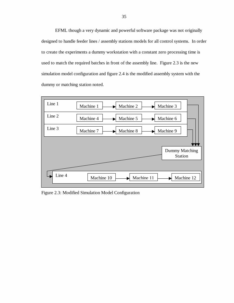
EFML though a very dynamic and powerful software package was not originally
designed to handle feeder lines / assembly stations models for all control systems. In order
to create the experiments a dummy workstation with a constant zero processing time is
used to match the required batches in front of the assembly line. Figure 2.3 is the new
simulation model configuration and figure 2.4 is the modified assembly system with the
dummy or matching station noted.
Figure 2.3: Modified Simulation Model Configuration
Line 3 Machine 7 Machine 9Machine 8
Line 2 Machine 4 Machine 6Machine 5
Line 1 Machine 1 Machine 3Machine 2
Line 4 Machine 10 Machine 12Machine 11
Dummy MatchingStation

36
Figure 2.4: EFML Simulation Model
2.2.1 Experimental Conditions
The following control parameter settings were used throughout the experiments.
• The processing times on each nonbottleneck machine follows an exponential
distribution with a mean of 25 seconds per item.
• The processing times on each bottleneck machine follows an exponential
distribution with a mean of 30 seconds per item.
• The batch size is 10 items.
• In order to reach equilibrium conditions, each experiment was run until 4000
batches were produced.
Machine Object
Matching Station
Dispatch Object
Setup Object

37
• There is an infinite amount of demand.
• There is an infinite supply of raw materials.
• Setup times are assumed to be zero for all batches and operations.
• Transportation time of a batch between two stations is instantaneous.
• The system components are 100% reliable with no breakdowns.
2.2.2 Calculations
Cycle Time
Cycle Time of Line 1 = Σ(cycle times of machines 1, 2, 3)
Cycle Time of Line 2 = Σ (cycle times of machines 4, 5, 6)
Cycle Time of Line 3 = Σ (cycle times of machines 7, 8, 9)
Cycle Time of Line 4 = Σ (cycle times of machines 10, 11, 12)
System Cycle time* = maximum (Feeder Line Cycle Times) + Cycle Time of
Line 4
*If line 2 and / or 3 follow the pull style production rules, the line’s cycle times are
not included in the formulation.
Final Inventory Status
This calculation serves the purpose of monitoring how many batches from a feeder
line are left unmatched at the dummy station after 4000 batches are produced by the
system. Here Nj is the number of items produced by Line j.
Unmatched Inventory at Line j = Nj – minimum (N1, N2, N3)
}3,2,1{∈j

38
CHAPTER 3
FEEDER LINE ANALYSIS
Hypothesis tests, with an α level of 0.05, were carried out on all of the feeder line
systems to determine the relationship of the samples’ parameters mean and variance with
each other. The parameters under consideration are throughput, WIP, and cycle time.
The throughput and WIP values represent the average throughput and WIP of sixteen
trials where each trial produced 4000 batches. The cycle time is the average cycle time of
4000 batches.
Administration of the hypothesis tests followed the procedure in figure 3.1.
3.1 MRP Feeder Lines
The MRP feeder lines contain three variables that affect the performance
indicators: the amount and location of the bottlenecks, and the interarrival time of raw
material to the feeder line. To identify the effects of the bottleneck and the interarrival
time, two separate analyses were carried out for each parameter. In the first section the
interarrival time of the raw material is held constant while the bottleneck locations are
varied, and in the second section the bottleneck location is held constant while the
interarrival times of the raw material is varied.

39
Figure 3.1: Analyst Procedure
Throughput Analysis of 3 Machine Lines
0.194
0.195
0.196
0.197
0.198
0.199
1 2 3 1, 2 1, 3 2, 3
Bottleneck Location
Ob
serv
ed T
hro
ug
hp
ut
(Bat
ches
/M
inu
te)
300
301
302
303
304
305
306
307
Figure 3.2: Throughput Analysis of 3 Machine MRP Lines– Interarrival Time Constant
Test if variances areequal between sample’sparameters
Variances arenot equal
Variances areequalIf sample size is
greater than 30 useZ statistic
If sample size is less than 30 use Tstatistic with unequal variances anddetermine appropriate degrees offreedom
If sample size is less than 30 use Tstatistic with equal variances anddetermine appropriate degrees offreedom
Analyze grouped data, check forpatterns in acceptance andrejection of null hypothesis
40
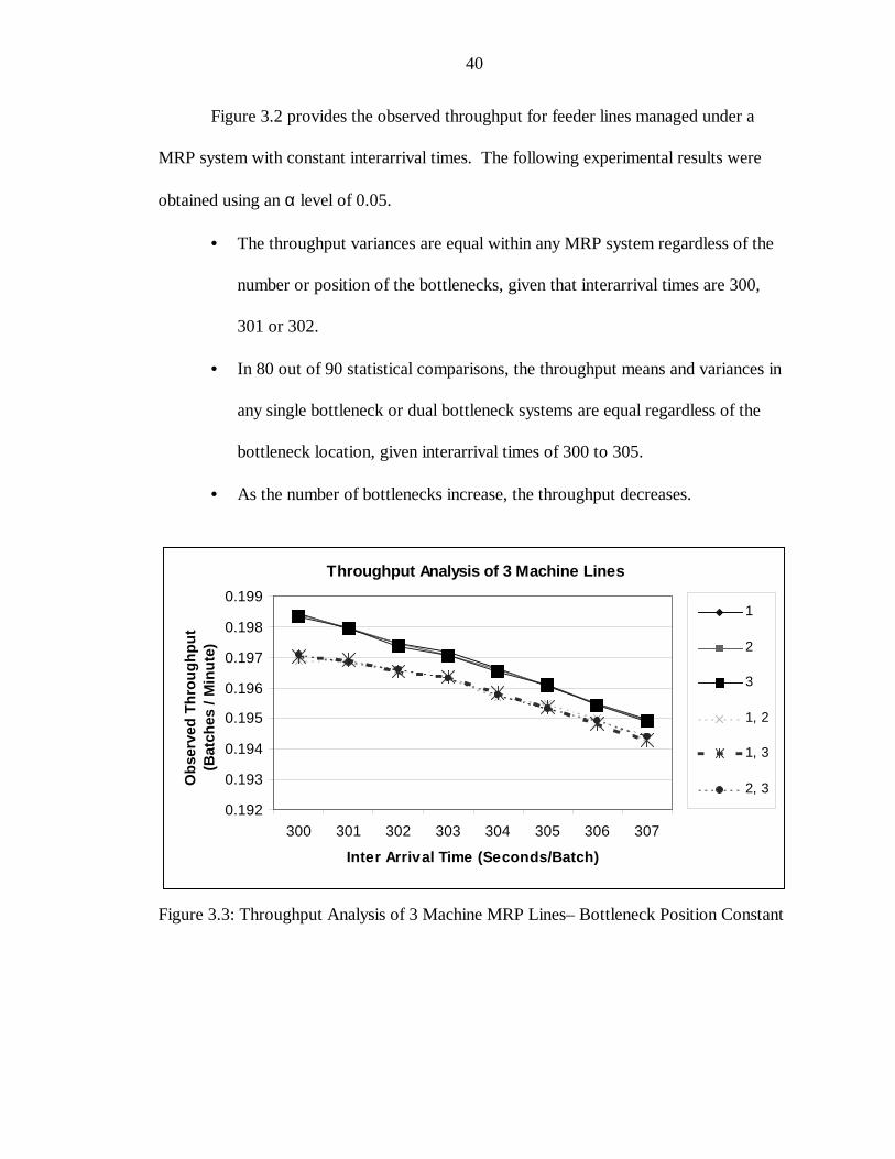
Figure 3.2 provides the observed throughput for feeder lines managed under a
MRP system with constant interarrival times. The following experimental results were
obtained using an α level of 0.05.
• The throughput variances are equal within any MRP system regardless of the
number or position of the bottlenecks, given that interarrival times are 300,
301 or 302.
• In 80 out of 90 statistical comparisons, the throughput means and variances in
any single bottleneck or dual bottleneck systems are equal regardless of the
bottleneck location, given interarrival times of 300 to 305.
• As the number of bottlenecks increase, the throughput decreases.
Figure 3.3: Throughput Analysis of 3 Machine MRP Lines– Bottleneck Position Constant
Throughput Analysis of 3 Machine Lines
0.192
0.193
0.194
0.195
0.196
0.197
0.198
0.199
300 301 302 303 304 305 306 307
Inter Arrival Time (Seconds/Batch)
Ob
serv
ed T
hro
ug
hp
ut
(Bat
ches
/ M
inu
te)
1
2
3
1, 2
1, 3
2, 3
41
Figure 3.3 provides the observed throughput for feeder lines managed under a
MRP system with constant bottleneck locations. The following experimental results were
obtained using an α level of 0.05.
• The throughput variances of MRP systems are equal at interarrival times of
300, 301, and 302, given identical bottleneck positions.
• The throughput means of MRP systems either remains unchanged or decreases
as interarrival times increase.
WIP Analysis of 3 Machine Lines
4
6
8
10
12
14
16
18
20
1 2 3 1, 2 1, 3 2, 3
Bottleneck Location
Ob
serv
ed W
IP (
Bat
ches
)
300
301
302
303
304
305
306
307
Figure 3.4: WIP Analysis of 3 Machine MRP Lines – Interarrival Time Constant
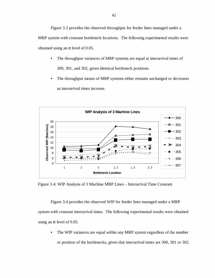
Figure 3.4 provides the observed WIP for feeder lines managed under a MRP
system with constant interarrival times. The following experimental results were obtained
using an α level of 0.05.
• The WIP variances are equal within any MRP system regardless of the number
or position of the bottlenecks, given that interarrival times are 300, 301 or 302.

42
• In 75 out of 90 statistical comparisons, the WIP means and variances in any
single bottleneck or dual bottleneck systems are equal regardless of the
bottleneck location, given interarrival times of 300 to 305.
• As the number of bottlenecks increase, the WIP increases.
WIP Analysis of 3 Machine Lines
4
6
8
10
12
14
16
18
20
300 301 302 303 304 305 306 307
Raw Material Arrival Time (Seconds/Batch)
Ob
serv
ed W
IP (
Bat
ches
)
1
2
3
1, 2
1, 3
2, 3
Figure 3.5: WIP Analysis of 3 Machine MRP Lines– Bottleneck Position Constant
Figure 3.5 provides the observed WIP for feeder lines managed under a MRP
system with constant bottleneck locations. The following experimental results were
obtained using an α level of 0.05.
• The WIP variances of MRP systems are equal at interarrival times of 300, 301,
and 302, given identical bottleneck positions.
• The WIP means of MRP systems either remains unchanged or decreases as the
interarrival times increase.

43
Cycle Time Analysis of 3 Machine Lines
0
2000
4000
6000
8000
10000
12000
1 2 3 1, 2 1, 3 2, 3Bottleneck Location
Cyc
le T
ime
(S
eco
nd
s/B
atch
)
300
301
302
303
304
305
306
307
Figure 3.6: Cycle Time Analysis of 3 Machine MRP Lines– Interarrival Time Constant
Figure 3.6 provides the observed cycle time for feeder lines managed under a MRP
system with constant interarrival times. The interarrival time of 300, as shown in figures
3.4a and 3.4b does exhibit anomalous behavior. The following experimental results were
obtained using an α level of 0.05.
• In 68 out of 72 statistical comparisons, increasing the number of bottlenecks
increases the cycle time mean.
• There is no discernible statistical pattern indicating that the position of the
bottleneck influences the cycle time mean of the MRP system.

44
Cycle Time Analysis of 3 Machine Lines
0
2000
4000
6000
8000
10000
12000
300 301 302 303 304 305 306 307
Interarrival Time
Cyc
le T
ime
(S
eco
nd
s /
Ba
tch
)
1
2
3
1, 2
1, 3
2, 3
Figure 3.7: Cycle Time Analysis of 3 Machine MRP Lines– Bottleneck Position Constant
Figure 3.7 provides the observed cycle time for feeder lines managed under a MRP
system with constant bottleneck locations. The interarrival time of 300, as shown in
figures 3.4a and 3.4b does exhibit anomalous behavior. The following experimental result
was obtained using an α level of 0.05. In 111 out of 126 statistical comparisons,
increasing the interarrival times of raw material reduce or maintain the cycle time mean.
3.2 Kanban Feeder Lines
The kanban feeder lines contain five variables that affect the performance
indicators: the number and locations of the bottlenecks, and the number of cards allocated
to each workstation. Each workstation has either one or two kanban cards allocated. To
identify the effects of the bottleneck and the card allocation, two separate analyses were
carried out for each parameter. In the first section the card allocation is held constant

45
while the bottleneck locations are varied, and in the second section the bottleneck location
is held constant while kanban card allocation is varied.
Throughput Analysis of 3 Machine Lines
0.160
0.165
0.170
0.175
0.180
0.185
0.190
0.195
0.200
1 2 3 1, 2 1, 3 2, 3
Bottleneck Location
Ob
serv
ed T
hro
ug
hp
ut
(B
atch
es /
Min
ute
)
1-1-1
1-1-2
1-2-1
2-1-1
1-2-2
2-1-2
2-2-1
2-2-2
Figure 3.8: Throughput Analysis of 3 Machine Kanban Lines– Card Allocation Constant
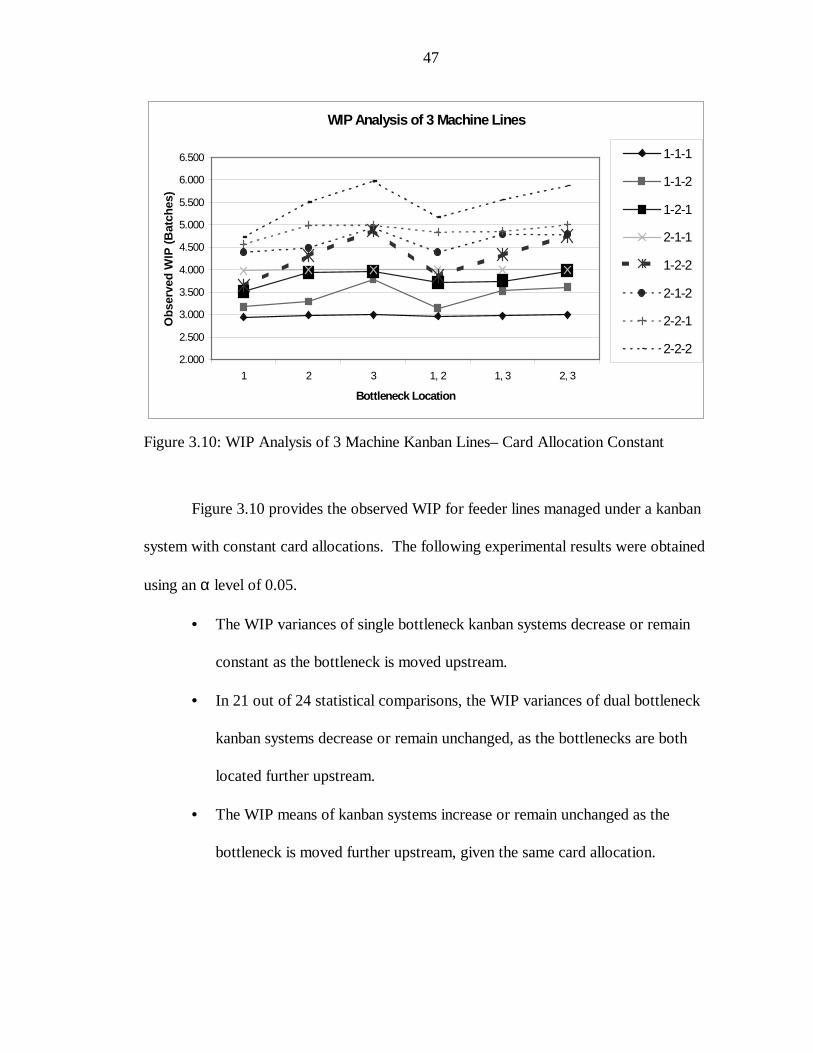
Figure 3.8 provides the observed throughput for feeder lines managed under a
kanban system with constant card allocations. The following experimental results were
obtained using an α level of 0.05.
• In 114 out of 120 statistical comparisons, the throughput variances of the
kanban systems are equal regardless of bottleneck position, given identical card
allocations.
• As the number of bottlenecks increase the throughput means decrease, given
identical card allocations.

46
• The throughput means increase for single bottleneck kanban systems in the
following cases: if an extra card is associated with the bottleneck station; if an
extra card is associated with the workstation prior to the bottleneck station; or
if the bottleneck is located at the initial workstation.
Figure 3.9: Throughput Analysis of 3 Machine Kanban Lines– Bottleneck PositionConstant
Figure 3.9 provides the observed throughput for feeder lines managed under a
kanban system with constant bottleneck locations. The following experimental result was
obtained using an α level of 0.05. As additional cards are allocated to the system, the
throughput means increase or remain constant, given identical bottleneck locations.
Throughput Analysis of 3 Machine Lines
0.160
0.165
0.170
0.175
0.180
0.185
0.190
0.195
0.200
1-1-1 1-1-2 1-2-1 2-1-1 1-2-2 2-1-2 2-2-1 2-2-2
Card Allocation
Ob
serv
ed T
hro
ug
hp
ut
(Bat
ches
/ M
inu
te)
1
2
3
1, 2
1, 3
2, 3
47
WIP Analysis of 3 Machine Lines
2.000
2.500
3.000
3.500
4.000
4.500
5.000
5.500
6.000
6.500
1 2 3 1, 2 1, 3 2, 3
Bottleneck Location
Ob
serv
ed W
IP (
Bat
ches
)1-1-1
1-1-2
1-2-1
2-1-1
1-2-2
2-1-2
2-2-1
2-2-2
Figure 3.10: WIP Analysis of 3 Machine Kanban Lines– Card Allocation Constant
Figure 3.10 provides the observed WIP for feeder lines managed under a kanban
system with constant card allocations. The following experimental results were obtained
using an α level of 0.05.
• The WIP variances of single bottleneck kanban systems decrease or remain
constant as the bottleneck is moved upstream.
• In 21 out of 24 statistical comparisons, the WIP variances of dual bottleneck
kanban systems decrease or remain unchanged, as the bottlenecks are both
located further upstream.
• The WIP means of kanban systems increase or remain unchanged as the
bottleneck is moved further upstream, given the same card allocation.

48
WIP Analysis of 3 Machine Lines
2.000
2.500
3.000
3.500
4.000
4.500
5.000
5.500
6.000
6.500
1-1-1 1-1-2 1-2-1 2-1-1 1-2-2 2-1-2 2-2-1 2-2-2
Card Allocation
Ob
serv
ed W
IP (
Bat
ches
)
1
2
3
1, 2
1, 3
2, 3
Figure 3.11: WIP Analysis of 3 Machine Kanban Lines– Bottleneck Position Constant
Figure 3.11 provides the observed WIP for feeder lines managed under a kanban
system with constant bottleneck locations. The following experimental result was
obtained using an α level of 0.05. In 112 out of 114 statistical comparisons, increasing the
number of cards in the systems increase WIP means, given identical bottleneck locations.

49
Cycle Time Analysis of 3 Machine Lines
600
800
1000
1200
1400
1600
1800
2000
1 2 3 1, 2 1, 3 2, 3Bottleneck Location
Cyc
le T
ime
(S
eco
nd
s /
Ba
tch
)1-1-1
1-1-2
1-2-1
1-2-2
2-1-1
2-1-2
2-2-1
2-2-2
Figure 3.12: Cycle Time Analysis of 3 Machine Kanban Lines– Card Allocation Constant
Figure 3.12 provides the observed cycle time for feeder lines managed under a
kanban system with constant card allocations. The following experimental results were
obtained using an α level of 0.05.
• The cycle time means of the system increase as the bottleneck stations move
further downstream, given identical card allocation.
• The cycle time means of single bottleneck kanban systems with the bottleneck
on the final workstation, is less than the cycle time of dual bottleneck kanban
systems with the initial bottleneck on the first workstation.

50
Cycle Time Analysis of 3 Machine Lines
600
800
1000
1200
1400
1600
1800
2000
1-1-1 1-1-2 1-2-1 2-1-1 1-2-2 2-1-2 2-2-1 2-2-2Card Allocation
Cyc
le T
ime
(S
eco
nd
s /
Bat
ch)
1
2
3
1, 2
1, 3
2, 3
Figure 3.13: Cycle Time Analysis of 3 Machine Kanban Lines– Bottleneck PositionConstant
Figure 3.13 provides the observed WIP for feeder lines managed under a kanban
system with constant bottleneck positions. The following experimental result was
obtained using an α level of 0.05. In 125 out of 132 statistical comparisons, increasing the
number of cards in the systems increase the cycle time means, given identical bottleneck
location.
3.3 CONWIP Feeder Line
The CONWIP feeder lines contain three variables that effect the performance
indicators: the number and position of the bottlenecks, and the number of cards allocated.
Unlike the other systems analyzed, the WIP is held constant as defined by the number of
cards allocated. To identify effects of the bottleneck and the number of cards allocated,
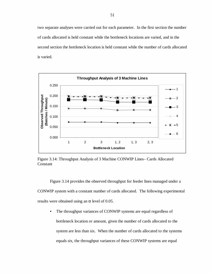
51
two separate analyses were carried out for each parameter. In the first section the number
of cards allocated is held constant while the bottleneck locations are varied, and in the
second section the bottleneck location is held constant while the number of cards allocated
is varied.
Figure 3.14: Throughput Analysis of 3 Machine CONWIP Lines– Cards AllocatedConstant
Figure 3.14 provides the observed throughput for feeder lines managed under a
CONWIP system with a constant number of cards allocated. The following experimental
results were obtained using an α level of 0.05.
• The throughput variances of CONWIP systems are equal regardless of
bottleneck location or amount, given the number of cards allocated to the
system are less than six. When the number of cards allocated to the systems
equals six, the throughput variances of these CONWIP systems are equal
Throughput Analysis of 3 Machine Lines
0.000
0.050
0.100
0.150
0.200
0.250
1 2 3 1, 2 1, 3 2, 3
Bottleneck Location
Ob
serv
ed T
hro
ug
hp
ut
(Bat
ches
/ M
inu
te)
1
2
3
4
5
6

52
regardless of bottleneck location, provided the systems have same number of
bottlenecks.
• The throughput means of CONWIP systems increase as the number of cards
allocated to the system increases.
• The throughput means of single bottleneck CONWIP systems having five cards
allocated are equal to the throughput means of single bottleneck CONWIP
systems with six cards, given identical number of cards allocated.
• The throughput means of CONWIP systems are equal, given identical number
of bottlenecks and cards allocated.
• The throughput means of CONWIP systems decrease as the number of
bottlenecks increase, given identical number of cards allocated.
Figure 3.15: Throughput Analysis of 3 Machine CONWIP Lines– Bottleneck PositionConstant
Throughput Analysis of 3 Machine Lines
0.050
0.070
0.090
0.110
0.130
0.150
0.170
0.190
0.210
1 2 3 4 5 6Number of Cards Allocated
Ob
serv
ed T
hro
ug
hp
ut
(Bat
ches
/Min
ute
) 1
2
3
1, 2
1, 3
2, 3
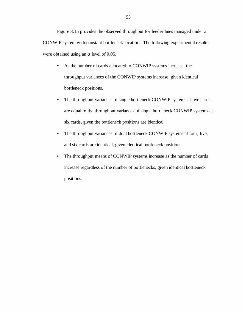
53
Figure 3.15 provides the observed throughput for feeder lines managed under a
CONWIP system with constant bottleneck location. The following experimental results
were obtained using an α level of 0.05.
• As the number of cards allocated to CONWIP systems increase, the
throughput variances of the CONWIP systems increase, given identical
bottleneck positions.
• The throughput variances of single bottleneck CONWIP systems at five cards
are equal to the throughput variances of single bottleneck CONWIP systems at
six cards, given the bottleneck positions are identical.
• The throughput variances of dual bottleneck CONWIP systems at four, five,
and six cards are identical, given identical bottleneck positions.
• The throughput means of CONWIP systems increase as the number of cards
increase regardless of the number of bottlenecks, given identical bottleneck
positions.
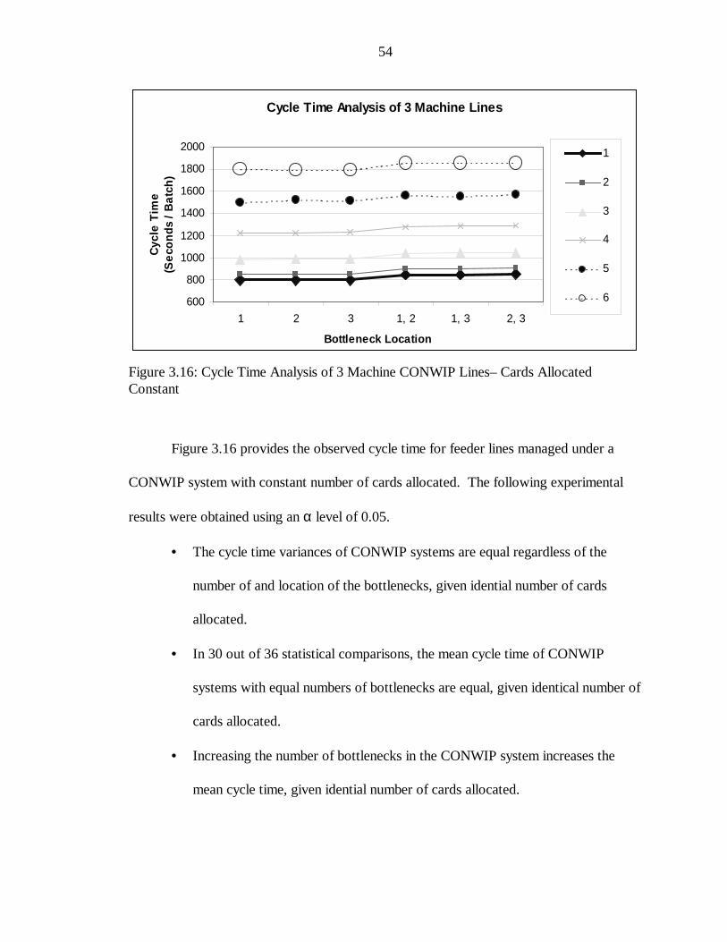
54
Cycle Time Analysis of 3 Machine Lines
600
800
1000
1200
1400
1600
1800
2000
1 2 3 1, 2 1, 3 2, 3
Bottleneck Location
Cyc
le T
ime
(S
eco
nd
s /
Ba
tch
)1
2
3
4
5
6
Figure 3.16: Cycle Time Analysis of 3 Machine CONWIP Lines– Cards AllocatedConstant
Figure 3.16 provides the observed cycle time for feeder lines managed under a
CONWIP system with constant number of cards allocated. The following experimental
results were obtained using an α level of 0.05.
• The cycle time variances of CONWIP systems are equal regardless of the
number of and location of the bottlenecks, given idential number of cards
allocated.
• In 30 out of 36 statistical comparisons, the mean cycle time of CONWIP
systems with equal numbers of bottlenecks are equal, given identical number of
cards allocated.
• Increasing the number of bottlenecks in the CONWIP system increases the
mean cycle time, given idential number of cards allocated.

55
Cycle Time Analysis of 3 Machine Lines
600
800
1000
1200
1400
1600
1800
2000
1 2 3 4 5 6
Number of Cards Allocated
Cyc
le T
ime
(Seco
nds /
Bat
ch)
1
2
3
1, 2
1, 3
2, 3
Figure 3.17: Cycle Time Analysis of 3 Machine CONWIP Lines– Bottleneck PositionConstant
Figure 3.17 provides the observed cycle time for feeder lines managed under a
CONWIP system with constant bottleneck locations. The following experimental results
were obtained using an α level of 0.05.
• Increasing the amount of cards allocated increases the cycle time variances,
given identical bottleneck positions.
• As the number of cards increase, the cycle time means also increase regardless
of the bottleneck postions.
3.4 Feeder Line Production Control Systems Summary and Conclusions of Findings
The basic findings of the feeder line analysis is that under any pure production
control system increasing the number of bottlenecks generally increases WIP, and cycle
time, and decreases throughput. This is an expected finding since the addition of the

56
bottleneck to the system automatically increases cycle time. Utilizing Little’s law given
constant WIP and increased cycle time results in deceased throughput, and given constant
throughput and increased cycle time results in increased WIP.
In push and pull systems starving the bottleneck station results in the system’s
throughput being reduced. In push systems bottleneck starvation can occur when raw
material is not delivered to the feeder lines fast enough. Therefore, as the interarrival
times are increased the throughput of the system decreases. In pull systems bottleneck
starvation can occur if the kanban cards are not allocated optimally. Therefore, as
additional cards are added to the system throughput increases. In a pull system, when the
bottleneck is starved the addition of cards will generally increase cycle time, WIP, and
throughput. An additional card decreases the amount of time the bottleneck is starved
thus results in an increase in throughput. The additional card also increases the maximum
number of batches in the system, and since more batches are in the system to be
processed, the cycle time increases.
The feeder analysis also indicates a reduction in system variance as the bottleneck
is moved downstream. Since the simulation uses an exponential distribution as a unit
mean process time distribution, moving the bottleneck station downstream would have the
same effect of moving a higher variable workstation downstream, and thus moving a
bottleneck station downstream can reduce system variation.
The analyses of the three production methodologies revealed characteristics of the
MRP and CONWIP systems that made them ideal for the analyses of assembly systems.
The MRP feeder lines’ throughput and WIP have equal mean and variance
regardless of bottleneck location, given identical number of bottlenecks and interarrival

57
times of 300 to 305. Additionally the MRP feeder lines show no discernable statistical
pattern that indicates that the position of the bottleneck influences the cycle time. Since
the interarrival time of raw material, not the location of the bottleneck, affects the
throughput and WIP, any alteration of the assembly system’s throughput and WIP using a
constant interarrival time is the result of the assembly station or the bottleneck’s position
relative to the assembly station.
The CONWIP system feeder lines’ throughput and cycle time are equal in mean
and variance regardless of the bottleneck postion given identical number of cards. In the
kanban system the allocation of the cards in relationship to the bottleneck influences
throughput. Since it is desireable in this paper to observe the effects of the bottleneck in
relation to the assembly station and not the effects of the bottleneck in relation to the
allocation of cards, the CONWIP production system will be used in constructing the pull
portion of the assembly systems.

58
CHAPTER 4
ASSEMBLY SYSTEM ANALYSIS
There are four full assembly systems under analysis: a pure push assembly system
with a batch synchronization procedure, a pure push assembly system without a batch
synchronization procedure, a pull-push system, and a hybrid pull/push-push system. Each
assembly system will be fully described prior to its respective analysis.
The feeder lines used in the construction of the assembly system had to have at
least an average throughput of 0.197 batches per minute. The throughput rate chosen is
the maximum throughput attainable from the MRP feeder line systems without
experiencing exploding inventories. The maximum throughput rate occurred at the
interarrival times of 300 and 301. The interarrival time of 301 was chosen to reduce WIP.
Since the assembly system study includes two bottlenecks, different card allocations must
be assigned to the CONWIP feeder lines with different amounts of bottlenecks. To
achieve at least 0.197 for the CONWIP feeder lines four cards were allocated when there
was no bottlenecks, six cards were allocated when there was one bottleneck, and thirteen
cards were allocated when there were two bottlenecks.
The assembly system is broken into three distinct segments: the assembly line, the
bottleneck feeder lines and the nonbottleneck feeder lines. The assembly line follows the
production control rules of a push system. The bottleneck feeder lines follow either the
MRP production rules with an interarrival time of 301, or the CONWIP production rules
with card settings of six, or thirteen depending on the number of bottleneck stations in the
feeder line. The nonbottleneck feeder lines follow either the MRP production rules with
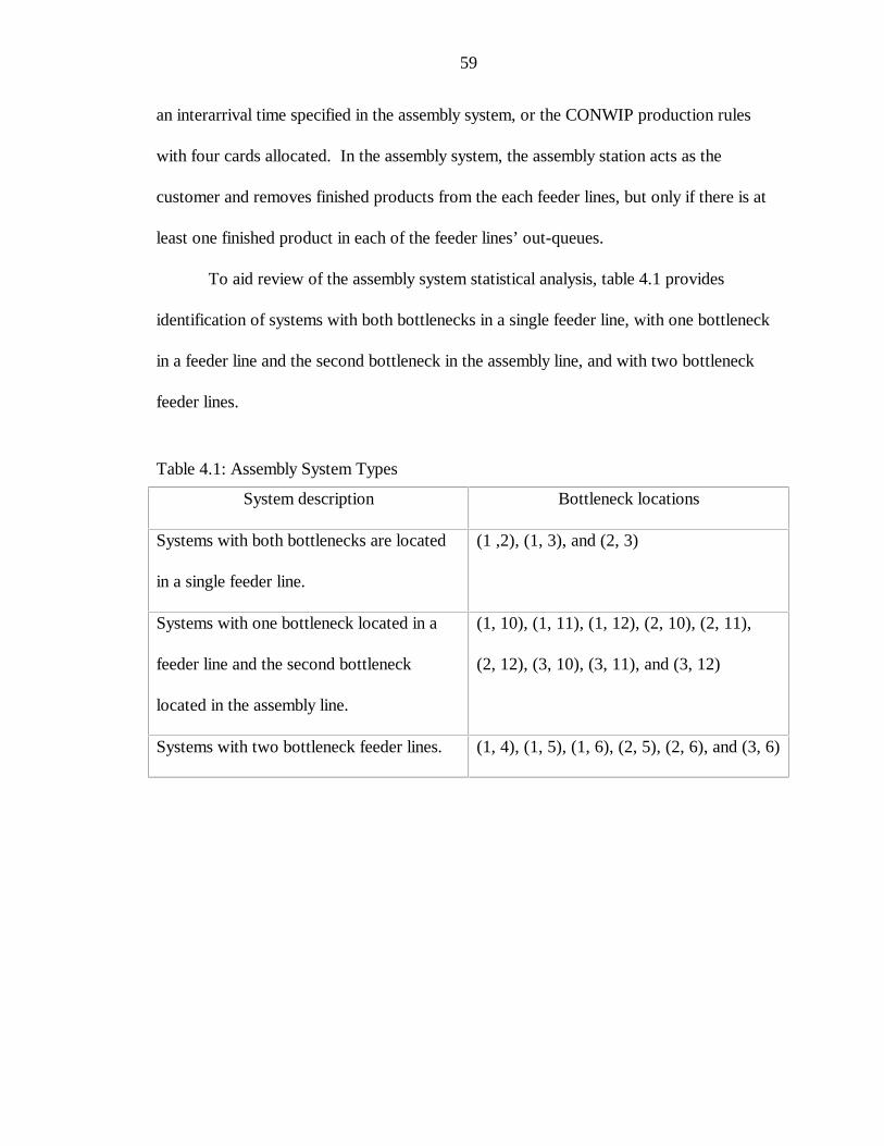
59
an interarrival time specified in the assembly system, or the CONWIP production rules
with four cards allocated. In the assembly system, the assembly station acts as the
customer and removes finished products from the each feeder lines, but only if there is at
least one finished product in each of the feeder lines’ out-queues.
To aid review of the assembly system statistical analysis, table 4.1 provides
identification of systems with both bottlenecks in a single feeder line, with one bottleneck
in a feeder line and the second bottleneck in the assembly line, and with two bottleneck
feeder lines.
Table 4.1: Assembly System Types
System description Bottleneck locations
Systems with both bottlenecks are located
in a single feeder line.
(1 ,2), (1, 3), and (2, 3)
Systems with one bottleneck located in a
feeder line and the second bottleneck
located in the assembly line.
(1, 10), (1, 11), (1, 12), (2, 10), (2, 11),
(2, 12), (3, 10), (3, 11), and (3, 12)
Systems with two bottleneck feeder lines. (1, 4), (1, 5), (1, 6), (2, 5), (2, 6), and (3, 6)

60
4.1 Pure Push Assembly Systems Using a Synchronization Process
This pure push production will serve as the base push assembly system. In this
system the interarrival times for the delivery raw material is set uniformly in all feeder lines
to 301. The batches entering the system in synchronization will combine at the assembly
station.
Throughput Analysis
0.1972
0.1974
0.1976
0.1978
0.198
0.1982
0.1984
0.1986
1,2
1,3
1,10
1,11
1,12 2,
3
2,10
2,11
2,12
3,10
3,11
3,12 1,
4
1,5
1,6
2,5
2,6
3,6
Bottleneck Location
Ob
serv
ed T
hro
ug
hp
ut
(Bat
ches
/ M
inu
te)
Figure 4.1: Throughput Analysis of Base Push Assembly System
Figure 4.1 provides the observed throughput for the push assembly system with
the batch synchronization process. The following experimental results were obtained
using an α level of 0.05.

61
• In 61 out of 66 statistical comparisons, the throughput variances of systems
with a single bottleneck feeder line are identical.
• The throughput variances of systems with two bottleneck feeder lines are
identical.
• The throughput means of systems with both bottlenecks in a single feeder line
are identical.
• The throughput means of systems with one bottleneck feeder line and the first
bottleneck in the first workstation are identical.
• The throughput means of systems with two bottleneck feeder lines are
identical.
Figure 4.2: WIP Analysis of Base Push Assembly System
WIP Analysis
15
20
25
30
35
40
45
1,2
1,3
1,10
1,11
1,12 2,3
2,10
2,11
2,12
3,10
3,11
3,12 1,4
1,5
1,6
2,5
2,6
3,6
Bottleneck Location
Ob
serv
ed W
IP (
Bat
ches
)

62
Figure 4.2 provides the observed WIP for the push assembly system with the batch
synchronization process. The following experimental results were obtained using an α
level of 0.05.
• The WIP variances of systems with bottlenecks located in two separate feeder
lines are identical.
• The WIP means of systems with both bottlenecks located in a single feeder line
are identical.
• The WIP means of systems with two bottleneck feeder lines are identical.
• If one bottleneck is located in a feeder line and the other one is in the assembly
line, then the WIP of these systems are identical.
• The WIP means of systems where one bottleneck is located in a feeder line and
the second bottleneck is located in the assembly line, are identical to the WIP
means of systems with both bottlenecks located in separate feeder lines.

63
Figure 4.3: Cycle Time Analysis of Base Push Assembly System
Figure 4.3 provides the observed cycle time for the push assembly system with the
batch synchronization process. No statistically discernable patterns were evident in cycle
time mean or variance at an α level of 0.05.
4.2 Pure Push Assembly Systems with No Synchronization Process
In the base push system synchronizing the sub-components for the assembly station
actually occurred when raw material was dispatched to the feeder lines. A consequence of
this action is the accumulation of batches in the nonbottleneck feeder lines’ out-queues.
This increase of system WIP ties in additional capital that could be used elsewhere.
In the DBR control system, the bottleneck is scheduled to ensure its complete
utilization. Thus the highest throughput is achieved while the WIP and cycle time of the
system is reduced. In the assembly system the assembly station does not necessarily need
Cycle Time Analysis
0
2000
4000
6000
8000
10000
12000
1,2 1,3 1,10 1,11 1,12 2,3 2,10 2,11 2,12 3,10 3,11 3,12 1,4 1,5 1,6 2,5 2,6 3,6
Bottleneck Location
Cyc
le T
ime
(Sec
on
ds
/ Bat
ch)

64
to be completely utilized, but the nonbottleneck feeder lines’ products should always be
available when the bottleneck feeder lines’ product becomes available. Using the DBR
methodology, this analysis attempted to balance the bottleneck and the nonbottleneck
feeder lines’ throughput in order to achieve decreased system WIP, without sacrificing
throughput. This was accomplished by gradually increasing the interarrival times of raw
material to the nonbottleneck feeder lines, while maintaining an interarrival time of 301 to
the bottleneck feeder lines.
The results indicate an interesting phenomenon at the assembly station that we
term as a pure-birth process. If the bottleneck feeder lines’ throughput differed from the
nonbottleneck feeder lines’ throughput, the difference would be the pure-birth process rate
of unmatched batches. To compute the total number of unmatched batches the “Final
Inventory Status” equation was used for each of the feeder lines.
To demonstrate how the pure-birth process can be hidden figures 4.4, 4.5, and 4.6
will be presented for assembly systems with one bottleneck feeder line and figures 4.7, 4.8,
and 4.9 will be presented for assembly systems with two bottleneck feeder lines. Figures
4.4 and 4.7 are the summed total of final inventories for the bottleneck feeder lines’
products. Figures 4.5 and 4.8 are the summed total of final inventories for the
nonbottleneck feeder lines’ products. The total final inventories of all the feeder lines’
products are in figures 4.6 and 4.9.
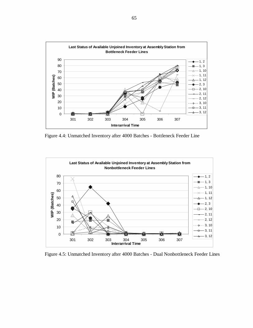
65
Figure 4.4: Unmatched Inventory after 4000 Batches - Bottleneck Feeder Line
Figure 4.5: Unmatched Inventory after 4000 Batches - Dual Nonbottleneck Feeder Lines
Last Status of Available Unjoined Inventory at Assembly Station from Bottleneck Feeder Lines
0
10
20
30
40
50
60
70
80
90
301 302 303 304 305 306 307
Interarrival Time
WIP
(B
atch
es)
1, 2
1, 3
1, 10
1, 11
1, 12
2, 3
2, 10
2, 11
2, 12
3, 10
3, 11
3, 12
Last Status of Available Unjoined Inventory at Assembly Station from Nonbottleneck Feeder Lines
0
10
20
30
40
50
60
70
80
301 302 303 304 305 306 307Interarrival Time
WIP
(B
atch
es)
1, 2
1, 3
1, 10
1, 11
1, 12
2, 3
2, 10
2, 11
2, 12
3, 10
3, 11
3, 12

66
Figure 4.6: Unmatched Inventory after 4000 Batches - Assembly Systems with OneBottleneck Feeder Line
Figure 4.7: Unmatched Inventory after 4000 Batches - Dual Bottleneck Feeder Lines
Last Status of Available Unmatched Inventory at Matching Station from All Feeder Lines
0
10
20
30
40
50
60
70
80
90
301 302 303 304 305 306 307Interarrival Time
WIP
(B
atch
es)
1, 2
1, 3
1, 10
1, 11
1, 12
2, 3
2, 10
2, 11
2, 12
3, 10
3, 11
Last Status of Available Unjoined Inventory at Assembly Station from Bottleneck Feeder Lines
0
20
40
60
80
100
120
140
160
180
301 302 303 304 305 306 307
Interarrival Time
WIP
(B
atch
es)
1, 4
1, 5
1, 6
2, 5
2, 6
3, 6

67
Figure 4.8: Unmatched Inventory after 4000 Batches - Nonbottleneck Feeder Line
Figure 4.9: Unmatched Inventory after 4000 Batches - Assembly Systems with TwoBottleneck Feeder Lines
Last Status of Available Unjoined Inventory at Assembly Station from Nonbottleneck Feeder Lines
0
2
4
6
8
10
12
14
16
301 302 303 304 305 306 307
Interarrival Time
WIP
(B
atch
es)
1, 4
1, 5
1, 6
2, 5
2, 6
3, 6
Last Status of Available Unmatched Inventory at Matching Station from All Feeder Lines
0
20
40
60
80
100
120
140
160
180
301 302 303 304 305 306 307Interarrival Time
WIP
(B
atch
es)
1, 4
1, 5
1, 6
2, 5
2, 6
3, 6

68
The pure-birth process is insidious in two manners. First, as illustrated in figures
4.4 and 4.7 this process can remain hidden. Second, as illustrated in figures 4.4, 4.5, 4.7,
and 4.8 the buildup of unmatched inventory appears to occur either in the bottleneck
feeder lines or the nonbottleneck feeder lines. In this analysis there does not appear to be
an interarrival time that the nonbottleneck feeder line can use, that will not generate
unmatched products. Because of the unchecked buildup of unmatched products at the
assembly station, unsynchronized assembly systems do not achieve steady state and thus
statistical analysis cannot be provided.
4.2.1 Process Analysis of Unmatched Feeder Line Inventory
TOC provides one major simplification for the proceeding analysis - subordinating
all processes to the bottleneck. The bottleneck feeder lines have the lowest throughput of
all the feeder lines. The assembly station requires the same amount of raw material from
each of the feeder lines; it cannot begin processing until this matched set is collected.
Since the joining process requires zero time, the arrival rate to the assembly station is
defined by the arrival rate (throughput) of products from the bottleneck feeder lines.
It is known that if the service rate of a process is less than the arrival rate, the
process’ queue will increase to infinity. If this occurs, the process is unstable and it can be
described as a birth process. Since the bottleneck feeder line’s throughput rate equals the
arrival rate of batches to the assembly station, the nonbottleneck feeder lines experience a
birth process.
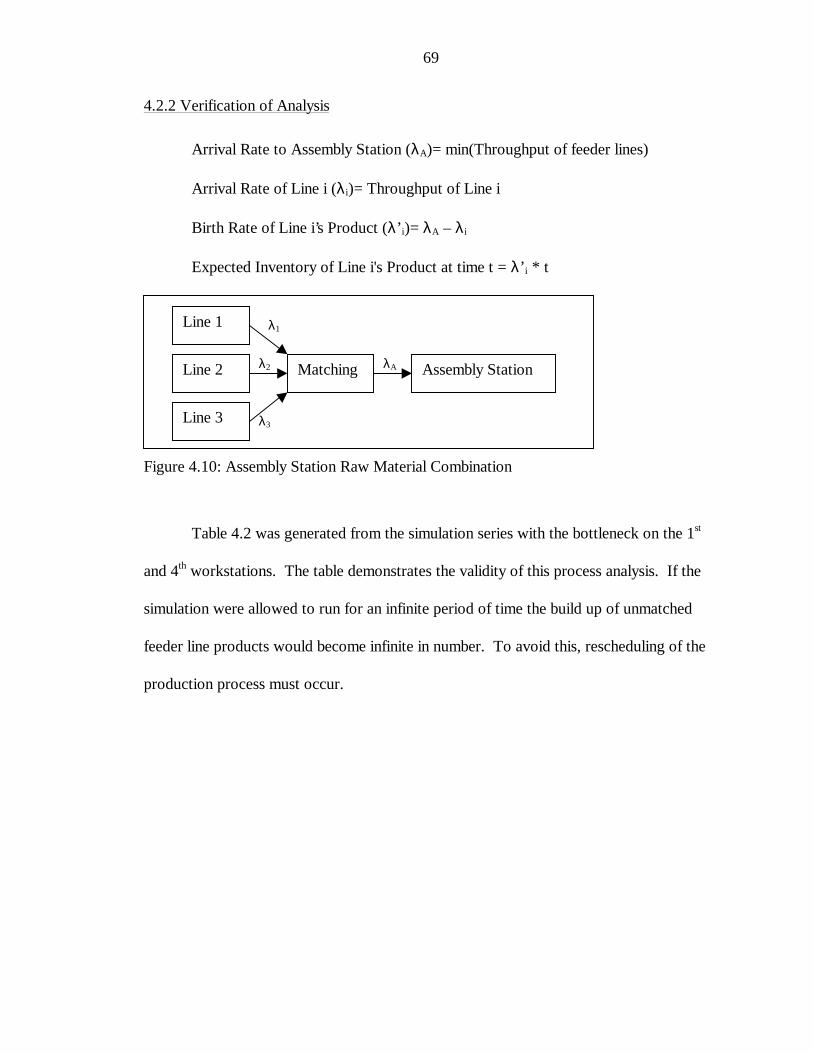
69
4.2.2 Verification of Analysis
Arrival Rate to Assembly Station (λA)= min(Throughput of feeder lines)
Arrival Rate of Line i (λi)= Throughput of Line i
Birth Rate of Line i’s Product (λ’ i)= λA – λi
Expected Inventory of Line i's Product at time t = λ’ i * t
Figure 4.10: Assembly Station Raw Material Combination
Table 4.2 was generated from the simulation series with the bottleneck on the 1st
and 4th workstations. The table demonstrates the validity of this process analysis. If the
simulation were allowed to run for an infinite period of time the build up of unmatched
feeder line products would become infinite in number. To avoid this, rescheduling of the
production process must occur.
λ1
λ2
λ3
λA
Line 1
Line 2
Line 3
Matching Assembly Station

70
Table 4.2: Series Comparison of Actual Feeder Line Inventory to the Predicted Value
Feeder Line Throughputs Feeder Line Birth RatesInterarrival Time 1 2 3 1 2 3
301 0.1991 0.1985 0.1993 0.0006 0.0000 0.0007302 0.1986 0.1985 0.1986 0.0001 0.0000 0.0000303 0.1992 0.1990 0.1979 0.0013 0.0011 0.0000304 0.1992 0.1990 0.1972 0.0020 0.0018 0.0000305 0.1991 0.1992 0.1966 0.0025 0.0026 0.0000306 0.1991 0.1990 0.1960 0.0031 0.0030 0.0000307 0.1980 0.1987 0.1954 0.0026 0.0033 0.0000
Time ofSimulation Run
Observed Final Inventory Expected Final Inventory
Seconds 1 2 3 1 2 31209874 11 0 15 11.3 0.0 15.01210431 1 0 0 2.1 0.0 0.91213771 26 23 0 25.3 22.7 0.01217855 41 36 0 41.1 35.9 0.01222144 50 53 0 50.0 52.6 0.01225511 64 62 0 64.3 62.3 0.01229527 54 69 0 53.2 68.6 0.0
The “Expected Final Inventory” was determined from the “Expected Inventory of
Line i” equation derived in section 4.2.and used the “Simulation Run Time” and the
“Feeder Line Birth Rates” as inputs.
4.3 Pull-Push Assembly Systems
Desiring to reduce the assembly system’s WIP and maintain throughput, the
CONWIP system is used to manage all feeder lines. When the synchronization of one
product from each of the feeder lines can occur, these items are joined together in a single
ten item batch and transported to the assembly station. Following the matching the cards

71
associated with the feeder lines’ products are released back to the initial workstations of
each respective feeder line.
The cards associated with each feeder line are dependent on the number of
bottlenecks resident therein. If no bottlenecks exist four cards are assigned to the feeder
line, if one bottleneck exists six cards are assigned to the feeder line, and if two
bottlenecks exist thirteen cards are assigned to the feeder line.
Figure 4.11: Throughput Analysis of Pull-Push Assembly System
Figure 4.11 provides the observed throughput for the pull-push assembly systems.
The following experimental results were obtained using an α level of 0.05.
• In 60 out of 66 statistical comparisons, the throughput variances of assembly
systems are equal.
• The throughput means of systems with both bottlenecks located in the same
feeder line are equal.
• The throughput means of systems with one bottleneck in the feeder lines are
equal.
Throughput Analysis
0.194
0.195
0.196
0.197
0.198
0.199
0.2
1,2
1,3
1,10
1,11
1,12 2,3
2,10
2,11
2,12
3,10
3,11
3,12 1,4
1,5
1,6
2,5
2,6
3,6
Bottleneck Location
Ob
serv
ed T
hro
ug
hp
ut
(Bat
ches
/ M
inu
te)

72
• The throughput means of assembly systems with both bottlenecks in one feeder
line are equal to or less than assembly systems with one bottleneck in the
feeder lines.
• The throughput means of systems with both bottlenecks in separate feeder lines
are equal.
• The throughput means of systems with both bottlenecks located in separate
feeder lines are less than the throughput means of systems with one bottleneck
feeder line.
Figure 4.12: WIP Analysis of Pull-Push Assembly System
Figure 4.12 provides the observed WIP for the pull-push assembly systems. The
following experimental results were obtained using an α level of 0.05.
• The WIP variances of systems with both bottlenecks in the same or different
feeder lines are equal.
• In 34 out of 45 statistical comparisons, the WIP variances of systems with one
bottleneck in the feeder lines are equal time.
WIP Analysis
05
10152025303540
1,2
1,3
1,10
1,11
1,12 2,3
2,10
2,11
2,12
3,10
3,11
3,12 1,4
1,5
1,6
2,5
2,6
3,6
Bottleneck Location
Ob
serv
ed W
IP (
Bat
ches
)

73
• The WIP variances of systems with one bottleneck in the feeder lines are
greater than systems with both bottlenecks located in one feeder line.
• In 39 out of 45 statistical comparisons, the WIP means of systems with one
bottleneck in the feeder lines are equal.
• The WIP means of systems with both bottlenecks in a single feeder line are less
than or equal to systems with only one bottleneck in the feeder lines.
• The WIP means of systems with both bottlenecks in separate feeder lines are
less than systems with the bottlenecks located elsewhere.
Cycle Time Analysis
0
2000
4000
6000
8000
10000
12000
1,2
1,3
1,10
1,11
1,12 2,3
2,10
2,11
2,12
3,10
3,11
3,12 1,4
1,5
1,6
2,5
2,6
3,6
Bottleneck Location
Cyc
le T
ime
(Sec
on
ds
/ Bat
ch)
Figure 4.13: Cycle Time Analysis of Pull-Push Assembly System
Figure 4.13 provides the observed cycle time for the pull-push assembly systems.
The following experimental results were obtained using an α level of 0.05.
• The cycle time variances of systems with both bottlenecks in one feeder line
are identical.
• The cycle time variances of systems with both bottlenecks in separate feeder
lines are identical.

74
• The cycle time variances of systems with both bottlenecks is separate feeder
lines are less than systems with the bottlenecks located elsewhere.
• The cycle times of systems with both bottlenecks in separate feeder lines are
less than in systems with the bottlenecks located elsewhere.
4.4 Hybrid Pull/Push-Push Assembly Systems
Desiring to further reduce the assembly system’s WIP and maintain throughput,
the DBR approach used in section 4.3 is re-evaluated. In that section scheduling the
arrival of nonbottleneck feeder lines’ product led to uncontrolled buildup of unmatched
product. To avoid this instabili ty the CONWIP system is used to manage the
nonbottleneck feeder lines. Spearman et al. [14] developed a similar method of using the
CONWIP and MRP production system rules to simulate a DBR system. The difference is
that Spearman used the system to manage a bottleneck station, and here the system
manages an assembly station.
As in section 4.3, when the synchronization of one product from each of the feeder
lines occurs, these batches are joined together in a single ten-item batch and transported to
the assembly station. Following the synchronization process the cards associated with the
nonbottleneck feeder lines’ products are released back to the initial workstations of the
nonbottleneck feeder lines. Four cards are allocated to the nonbottleneck feeder lines to
ensure the availabili ty of product at the assembly station.
Little’s Law is applicable in many situations, but because of how the cycle time is
defined for the assembly systems it seems to fail for the hybrid pull/push-push system. In
this system the cycle time is defined along the bottleneck feeder lines and the assembly

75
line. Changes to the nonbottleneck feeder lines’ WIP does not necessarily affect the
systems’ throughput or cycle time means, but will affect the systems’ WIP. If the cycle
time of the assembly systems were defined using the average of the feeder lines’ cycle
times, Little’s Law would apply.
Throughput Analysis
0.1978
0.1979
0.198
0.1981
0.1982
0.1983
0.1984
1,2
1,3
1,10
1,11
1,12 2,3
2,10
2,11
2,12
3,10
3,11
3,12 1,4
1,5
1,6
2,5
2,6
3,6
Bottleneck Location
Ob
serv
ed T
hro
ug
hp
ut
(Bat
ches
/ M
inu
te)
Figure 4.14: Throughput Analysis of Hybrid Pull/Push-Push System
Figure 4.14 provides the observed throughput for the hybrid pull/push-push
assembly systems. The following experimental results were obtained using an α level of
0.05.
• The throughput variances of systems with both bottlenecks in a single feeder
line are identical.
• The throughput variances of systems with two bottleneck feeder lines are
identical.

76
• In 152 out of 153 statistical comparisons, the throughput variances of systems
regardless of bottleneck location are identical.
• The throughput means of systems with one bottleneck on the first workstation
of a feeder line and second bottleneck in the assembly line are identical.
• The throughput means of systems with one bottleneck on the second
workstation of a feeder line and second bottleneck in the assembly line are
identical.
• The throughput means of systems with one bottleneck on the third workstation
of a feeder line and second bottleneck in the assembly line are identical.
• In 64 out of 66 statistical comparisons, the throughput means of systems with
one bottleneck feeder line are identical.
• The throughput means of systems with both bottlenecks located in separate
feeder lines are identical.
• The throughput means of systems with one bottleneck feeder line are less than
or equal to the throughput means of systems with two bottleneck feeder lines.

77
WIP Analysis
24
25
26
27
28
29
30
31
32
33
34
1,2
1,3
1,10
1,11
1,12 2,
3
2,10
2,11
2,12
3,10
3,11
3,12 1,
4
1,5
1,6
2,5
2,6
3,6
Bottleneck Location
Ob
serv
ed W
IP (
Bat
ches
)
Figure 4.15: WIP Analysis of Hybrid Pull/Push-Push System
Figure 4.15 provides the observed WIP for the hybrid pull/push-push assembly
systems. The following experimental results were obtained using an α level of 0.05.
• The WIP variances of systems with one bottleneck feeder line are identical.
• The WIP variances of systems with two bottleneck feeder lines are identical.
• In 147 out of 153 statistical comparisons, the WIP variances of systems with
two bottlenecks are identical.
• The WIP means of systems with two bottlenecks are equal regardless of the
number of feeder lines.

78
Cycle Time Analysis
0
1000
2000
3000
4000
5000
6000
7000
8000
9000
10000
1,2 1,3 1,10 1,11 1,12 2,3 2,10 2,11 2,12 3,10 3,11 3,12 1,4 1,5 1,6 2,5 2,6 3,6
Bottleneck Location
Cyc
le T
ime
(Sec
on
ds
/ Bat
ch)
Figure 4.16: Cycle Time Analysis of Hybrid Pull/Push-Push System
Figure 4.16 provides the observed cycle time for the hybrid pull/push-push
assembly systems. The following experimental results were obtained using an α level of
0.05.
• The cycle time variances of systems with one bottleneck on the first
workstation of a feeder line and the second bottleneck located in the assembly
line are identical.
• In 20 out of 21 statistical comparisons, the cycle time variances of systems
with one bottleneck on the second workstation of a feeder line and the second
bottleneck located in the assembly line are identical.
• If the first bottleneck is on the first workstation of the system, the cycle time
means increase as the second bottleneck moves further downstream.

79
4.5 Assembly System Summary and Conclusions of Findings
Much of the feeder line analysis can be used to predict the assembly systems’
responses to bottlenecks. In the feeder line analysis, increasing the number of bottlenecks
decreases throughput. In the assembly system analysis, increasing the number of
bottlenecks in the same feeder line decreases throughput. In the feeder line analysis, WIP
variance is zero in CONWIP systems while it is present in push systems. In the assembly
system analysis, systems using CONWIP techniques experience less WIP variability than
systems reliant purely on push systems.
Sometimes the feeder line analysis cannot be used to infer the results of assembly
systems’ responses to bottlenecks. If both bottlenecks are located in separate feeder lines,
the pull-push assembly systems experience a decrease in throughput. From the feeder line
analysis, it is known that both bottleneck feeder lines have identical throughputs. The loss
of throughput results from the probability of both bottleneck feeder lines finishing a
product at the same time being equal to zero. Even though all two bottleneck feeder line
assembly systems experience this batch matching delay only systems that manage the
bottleneck feeder lines with a pull system experience a significant reduction in throughput.
The pure push assembly systems provide impressive results in regards to
throughput and WIP. Statistically, the throughput means of these systems are not
necessarily identical but the difference between the maximum throughput and the
minimum throughput is 0.0007. The WIP means of the push systems are also consistent
with a difference only becoming evident when both bottlenecks are located in the same
feeder line. The pure push assembly system does have its shortcomings. It has the

80
potential to be unstable. To avoid this instability, the pure-birth process, this type of
assembly system requires the use of a batch synchronization procedure.
The pull-push assembly systems provide impressive results in regard to system
variability. In these assembly systems the throughput, WIP, and cycle time variances are
consistent regardless of the bottleneck locations. The throughput and WIP means are
effected by the positions of the bottleneck stations in relation to the assembly station. If
one bottleneck is in the assembly line the pull-push systems experience its greatest average
throughput and WIP; if both bottlenecks are in a single feeder line the throughput and
WIP are reduced; and if two bottleneck feeder lines exist the throughput and WIP are
significantly reduced.
The pull-push assembly system is significantly affected by the batch matching
delay. The additional wait time increases the bottleneck feeder lines’ cycle time and the
probability for the bottlenecks to starve. The combination of bottleneck starvation,
constant feeder line WIP, and increased bottleneck feeder line cycle time results in a
significant reduction in the assembly system’s throughput, WIP, and cycle time. Little’s
Law still applies. The law must be applied to the feeder and assembly lines separately.
The bottleneck feeder lines experience increased cycle time, while maintaining a constant
WIP. Using Little’s Law this combination results in lower feeder line throughput. The
assembly line now has an increased interarrival time between batches. The increased
interarrival time reduces the assembly lines’ WIP and cycle time. Apparently the reduction
in the assembly lines’ WIP and cycle time is greater than the increased WIP and cycle time
associated with a two bottleneck feeder line assembly system and batch matching delay
compared to systems with one bottleneck feeder line and no batch matching delay.

81
The hybrid pull/push-push systems provide superior results in regard to throughput
and WIP. Statistically, the throughput means of these systems are not necessarily identical
but the difference between the maximum throughput and the minimum throughput is
0.0006. Additionally the throughput variances and the WIP means and variances of these
systems are consistent. Since this system uses a push technique to manage the bottleneck
feeder lines, the batch matching delay does not have a noticeable effect. In fact, it is
shown that systems with two bottleneck feeder lines achieve greater throughput rates than
the hybrid systems with a single bottleneck feeder line. Thus, the delay experienced for
batch matching is less than the delay experienced at the second bottleneck located
downstream from the first bottleneck. The hybrid assembly system does have its
shortcomings. If the nonbottleneck feeder lines are not managed properly this system
could also experience a pure-birth process.

82
CHAPTER 5
ASSEMBLY SYSTEM COMPARISON ANALYSIS
Of the assembly systems originally analyzed, only the three systems that achieved
equilibrium are compared. The parameter settings of these systems were derived from the
feeder line analysis in chapter three. In chapter four it was determined that bottleneck
position does effects the performance indicators of assembly systems using a pull system
to manage the bottleneck feeder lines. Given the information in chapter three, it is known
that the pure push and hybrid assembly systems are achieving their optimal throughput
values. Given the information from chapter four, it is known that the pull-push systems
analyzed in this chapter are not at their optimal settings.
The following results are broken into three sections where comparisons between
the performance indicators are carried out. After the results this chapter is summarized.
Figures 5.1, 5.2, and 5.3 provide observed throughput, WIP, and cycle time means for the
assembly systems.
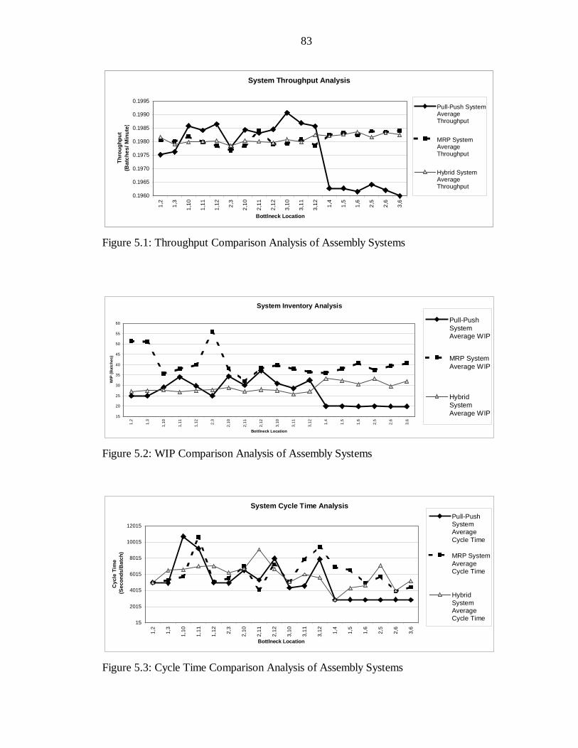
83
System Throughput Analysis
0.1960
0.1965
0.1970
0.1975
0.1980
0.1985
0.1990
0.1995
1,2
1,3
1,10
1,11
1,12 2,3
2,10
2,11
2,12
3,10
3,11
3,12 1,4
1,5
1,6
2,5
2,6
3,6
Bottlneck Location
Th
rou
gh
pu
t (B
atch
es/ M
inu
te)
Pull-Push SystemAverageThroughput
MRP SystemAverageThroughput
Hybrid SystemAverageThroughput
Figure 5.1: Throughput Comparison Analysis of Assembly Systems
System Inventory Analysis
15
20
25
30
35
40
45
50
55
60
1,2
1,3
1,10
1,11
1,12 2,
3
2,10
2,11
2,12
3,10
3,11
3,12 1,
4
1,5
1,6
2,5
2,6
3,6
Bottlneck Location
WIP
(B
atch
es)
Pull-PushSystemAverage WIP
MRP SystemAverage WIP
HybridSystemAverage WIP
Figure 5.2: WIP Comparison Analysis of Assembly Systems
System Cycle Time Analysis
15
2015
4015
6015
8015
10015
12015
1,2
1,3
1,10
1,11
1,12 2,3
2,10
2,11
2,12
3,10
3,11
3,12 1,4
1,5
1,6
2,5
2,6
3,6
Bottlneck Location
Cyc
le T
ime
(S
eco
nd
s/B
atch
)
Pull-PushSystemAverageCycle Time
MRP SystemAverageCycle Time
HybridSystemAverageCycle Time
Figure 5.3: Cycle Time Comparison Analysis of Assembly Systems
84
5.1 Push and Pull-Push Assembly Systems
The push and the pull-push assembly systems differ in that the push assembly
systems manage all the feeder lines with synchronized dispatches of raw material and the
pull-push assembly systems manage all the feeder lines with a CONWIP system. The
following experimental results were obtained using an α level of 0.05.
• The WIP means and variances of pull-push systems are less than the equivalent
push systems.
• The throughput means of pull-push assembly systems with one bottleneck
located in the assembly line are greater than or equal to the equivalent push
systems.
• The throughput means of pull-push assembly systems with both bottlenecks in
a single bottleneck feeder line are less than or equal to the equivalent push
assembly systems.
• The throughput means of pull-push assembly systems with two bottleneck
feeder lines are less than or equal to the equivalent push assembly systems.
• The cycle time variances of pull-push assembly systems with both bottlenecks
in a single bottleneck feeder line are less than the equivalent push assembly
systems.
• The cycle time means of pull-push assembly systems with two bottleneck
feeder lines are less than or equal to the equivalent push assembly systems.

85
5.2 Push and Hybrid Pull/Push-Push Assembly Systems
The push and the hybrid assembly systems differ in the following manner. Push
assembly systems manage the bottleneck and nonbottleneck feeder lines with synchronized
dispatches of raw material. Hybrid assembly systems manage the bottleneck feeder lines
with synchronized dispatches of raw material and the nonbottleneck feeder lines with
CONWIP systems. The following experimental results were obtained using an α level of
0.05.
• In 16 out of 18 statistical comparisons, the push and hybrid assembly systems
have equal throughput means and variances, given identical bottleneck
positions.
• The WIP means and variances of push assembly systems with both bottlenecks
in the same feeder line are greater than the equivalent hybrid systems.
• The cycle time variances of push and pull-push assembly systems with both
bottlenecks in a single feeder line are identical, given identical bottleneck
positions.
5.3 Hybrid and Pull-Push Assembly Systems
The pull-push and the hybrid assembly systems differ in the following manner.
Pull-push assembly systems manage the bottleneck and nonbottleneck feeder lines with
CONWIP systems. Hybrid assembly systems manage the bottleneck feeder lines with
synchronized dispatches of raw material and the nonbottleneck feeder lines with CONWIP
systems. The following experimental results were obtained using an α level of 0.05.

86
• The WIP means and variances of hybrid assembly systems are greater than the
equivalent pull-push assembly systems.
• The throughput means of hybrid assembly systems with one bottleneck in the
assembly line are less than or equal to the equivalent pull-push assembly
systems.
• The throughput means of hybrid assembly systems with two bottleneck feeder
lines are greater than the equivalent pull-push assembly systems.
• The cycle time variances of hybrid assembly systems with both bottlenecks in
one feeder line are identical to the equivalent pull-push assembly systems.
• The cycle time means of hybrid assembly systems with two bottleneck feeder
lines are greater than the equivalent pull-push assembly systems.
5.4 Assembly System Comparison Summary of Findings
The pull-push assembly system has demonstrated that it is capable of high levels of
throughput at reduced WIP. This assembly system has also demonstrated some of its
fallacies. If the number of cards allocated to the CONWIP system is insufficient to
properly ensure the bottleneck is always working, the systems experiences a loss in
throughput. Additionally the use of this assembly system’s management technique
requires additional cards assigned to the bottleneck feeder lines when there are two or
more bottleneck feeder lines feeding an assembly station.
The push and the hybrid assembly systems demonstrate equivalent throughputs.
But the hybrid assembly system is able to achieve those throughputs at lower levels of

87
WIP and variability than the push system. The similarity and dissimilarity of these systems
can be tied to how the hybrid system is constructed. The bottleneck feeder lines control
the throughput of the system. In both the push and hybrid systems these lines are
managed identically with a push systems. The nonbottleneck feeder lines in both of these
systems are managed to ensure that its product is always ready for the assembly station
when the bottleneck feeder lines’ product becomes available. In the push system this
management resulted in higher WIP and variability than when it is managed by the
CONWIP system.

88
CHAPTER 6
CONCLUSIONS
The factors that determine how well an assembly system performs are: types of
control systems are used; the amount and location of bottlenecks; and if a synchronization
process is implemented.
If the entire assembly system is managed via a push system, a synchronization
process must be implemented. If this does not occur the assembly system will become
unstable. In Agnetis’ [2] paper this instabili ty resulted in tardy jobs, in this paper the
instabili ty is the result of a pure-birth process occurring at the assembly station. The pure-
birth process was shown to exist in all unsynchronized push assembly systems studied. In
the unsynchronized push assembly system, WIP becomes unmanageable unless production
rescheduling is continually provided.
Managing the nonbottleneck feeder lines with a pull system can eliminate the need
for the synchronization process. In order to eliminate the need, the nonbottleneck feeder
lines are managed in such a way that if left unhindered will achieve a greater throughput
than the bottleneck feeder lines. Since the bottleneck feeder lines determine when the
nonbottleneck feeder lines release a card, the throughput and the WIP of the
nonbottleneck feeder lines remain in check. An additional advantage of managing the
nonbottleneck feeder lines with a pull system is reduced system WIP. Even with these
advantages, the hybrid pull/push-push control system does have its shortcomings. If the

89
nonbottleneck feeder lines are not managed properly, a pure-birth process will result.
Also, given that the nonbottleneck feeder lines are managed properly, the maximum
throughput attainable in the hybrid systems is identical to the equivalent assembly systems
managed by a synchronized push system.
Given that the flow lines are properly managed, to eliminate the possibility of a
pure-birth process, and to possibly achieve greater system throughput the bottleneck
feeder lines must also be managed by a pull system. In this analysis the pull-push assembly
system did not always achieve the highest throughput of the assembly systems, but its card
settings are not optimally set. The lost throughput can be overcome with additional cards
allocated.
The use of pull systems to manage the assembly station is derived from the TOC
philosophy. In this situation the assembly station is not necessarily the bottleneck, it is a
process that can potentially lead to infinite-sized buffers. This technique was derived after
observing the instability of unsynchronized push assembly systems.
Through the analysis performed in this paper, the following three statements have
been shown to be true for assembly systems. Given that the flow lines are in equilibrium,
by managing the assembly system with a push system, batch synchronization must occur to
prevent a pure-birth process from developing. Given that the flow lines are in equilibrium,
by managing the nonbottleneck feeder lines with a pull system, the WIP of the system can
be reduced. Given that the flow lines are in equilibrium, by managing all feeder lines with
a pull system, the WIP of the system can be reduced, a pure-birth process cannot occur,
and increased throughput may by achieved.

90
System robustness, the ability for the system to achieve equivalent production rates
(throughput) if the bottleneck station shifts location, is a critical factor in managing an
assembly system. If the bottleneck shifts within its feeder or assembly lines no significant
change in throughput is expected in any of the assembly systems examined. If the
bottleneck station shifts to a different flow line this results in a misidentification of the
bottleneck feeder line and can result in changes in the assembly systems’ throughput and
equilibrium status.
Misidentification of the bottleneck feeder line and thus the mismanagement of this
line can result in a birth process and / or lost system throughput. In the pure push
assembly system with batch synchronization (MRP system) shifting of the bottleneck
station to different flow lines will not significantly effect the systems’ throughput or
equilibrium. In the pull-push assembly system shifting of the bottleneck station to different
flow lines, without reallocation of system cards, can result in decreased system throughput
but equilibrium will be maintained. In the hybrid assembly system shifting of the
bottleneck station to different flow lines, without altering how the assembly system is
managed, can result in a combined decrease in system throughput and a pure-birth
process. Thus in regards to robustness, the pure push assembly system with batch
synchronization is the most stable, and the hybrid system is the least stable.
The findings indicate that prior to the implementation of production management
techniques to assembly systems. The system should be studied to determine the location
and any shifting properties of the bottleneck station or stations. If the bottleneck stations
regularly shift in regards to different flow lines a MRP management system may be the
most appropriate. If consistent nonbottleneck feeder lines exist, management of these

91
flow lines with CONWIP systems will reduce the system’s WIP and not effect the
system’s throughput. If the bottleneck station does not shift between flow lines,
management of all feeder lines with CONWIP systems can result in higher system
throughput and reduced system WIP.

92
GLOSSARY OF TERMS
This thesis uses a variety of terms that the reader may not be aware of or that
differ from literature source to literature source. These terms are defined when first used,
but are supplied here to aid the reader.
Term DefinitionAssembly Line A serial line of production stations with one or more
assembly stationsAssembly Station The station which two or more workstations feed with
different products. The products of the workstationsare then combined into a unique product.
Assembly System Production system containing one or more assemblystations.
Batch One or more units to be processed on a station that aregrouped together.
Bottleneck A machine whose throughput directly effects thethroughput of the system.
Bottleneck Feeder Line Feeder line containing a bottleneck station.Bottleneck Line Serial line of workstations with one or more
bottlenecks.Cycle Time The average time it takes for a batch to be processed on
the production system.Downstream A station or stations that proceeds the current station.Feeder Line Serial line whose end product is used at the assembly
stationSynchronization Process A synchronization process occurs when each
component used in the assembly station’s product wasintroduced to the manufacturing system to specificallycombine with one another.
Nonbottleneck Feeder Line Feeder line not containing a bottleneck station.Nonbottleneck Line Sequential production line without a bottleneck.Process Time The time it takes to product one unit of product.Production system The set of manufacturing processes that are required to
transform raw material into a end product.Raw Material The input to a production system.Throughput The number of units produced per unit of time. This

93
unit of measurement can be observed at the workstationor system level. The final workstation’s throughput isthe production systems throughput.
Upstream A station or stations that precede the current station.Work in Process Inventory at a workstation’s in-queue, out-queue, and
being processed.Workstation A production station with one input and one output per
product type.

94
LIST OF REFERENCES
[1] Altug, M. S. “Design and Performance Evaluation of Mixed MRP, Kanban, andCONWIP Production Systems Using Emulated Flexible ManufacturingLaboratory.” M.S. Thesis, University of Florida, Gainesville, 1997
[2] Agnetis, A., Pacifici, A., Rossi, F., Lucertini, M., Nicoletti, S., Nicolo, F., Oriolo, G.,Pacciarelli, D., & Pesaro, E. “Scheduling of flexible flow lines in an automobileassembly plant.” European Journal of Operations Research, Vol. 97, 348-362,1997
[3] Bonvik, A. M., Couch, C. E., & Gershwin, S. B. “A comparison of production-linecontrol mechanism” International Journal of Production Research, Vol. 35, No. 3,789-804, 1997
[4] Cook, D. P. “A simulation comparison of traditional, JIT, and TOC manufacturingsystems in a flow shop with bottlenecks.” Production and Inventory Management,Vol. 35, 73-78, 1994
[5] Dallery, Y., Liu, Z. & Towsley, D. “Properties of fork/join queuing networks withblocking under various operating mechanisms.” IEEE Transactions on Roboticsand Automation, Vol. 13, No. 4, 503-518, August 1997
[6] Gstettner, S. and Kuhn, K. “Analysis of production systems kanban and CONWIP.”International Journal of Production Research, Vol. 34, No. 11, 3253-3272, 1996
[7] Goldratt, E. The Goal: A Process of Ongoing Improvement, Great Barrington, MA:North River Press Inc 1984.
[8] Guide, V. D. R. “Scheduling using drum-buffer-rope in a remanufacturingenvironment” International Journal of Production Research, Vol. 34, No. 4, 1081-1091, 1996
[9] Huang, M. Wang, D. & Ip, W. H. “Simulation Study of CONWIP for a cold rollingplant.” International Journal of Production Economics, Vol. 54, 257-266, 1998
[10] Kleinrock L., Queuing Systems Volume I: Theory, New York: Wiley, 1976

95
[11] Krejewski, L.J., King, B.E. Ritzman, L. P., and Wong, D. S., “Kanban, MRP, andshaping the Manufacturing Environment.” Management Sciences, Vol. 33, 39-57,1987
[12] Luppen, R. T. Just-in-time Manufacturing New York: McGraw-Hill BookCompany, 1998
[13] Rao, S. S., Gunasekaran, A., Goyal, S. K., & Martinkainen, T. “Waiting line modelapplications in manufacturing.” International Journal of Production Economics,Vol. 54, 1-28, 1998
[14] Spearman, M. L. Woodruff, D., & Hopp, W. J. “CONWIP:a pull alternative tokanban.” International Journal of Production Research, Vol. 5, 879-894, 1990
[15] Spencer, M. S., & Cox III, J. F. “Master production scheduling development intheory of constraints environment.” Production and Inventory ManagementJournal, First Quarter, 8-13, 1995

96
BIOGRAPHICAL SKETCH
Tim Elftman was born in Cleveland, Ohio on January 24, 1973. Prior to finishing
high school, he attended Driffield School as an exchange student in England, from 1989 to
1990. In 1991, he graduated from Midview High School in Grafton, Ohio. In 1994, he
attained an Associate of Arts Degree in Engineering from Central Florida Community
College in Ocala, Florida. From 1995 to 1997, he attended the University of Florida and
specialized in industrial and systems engineering. After obtaining a Bachelor of Science
degree, he continued at the University of Florida further specializing in operations research
at the Department of Industrial and Systems Engineering. He will receive a Master of
Science degree from this department in May of 1999.