EVs, Low Carbon Fuels, and a Technology-Neutral Playing Field

Presented to: 34th Annual ACE Conference

August 20, 2021

Steffen Mueller, PhD Principal Economist

UIC Energy Resources Center

Overview

Two Recent UIC Studies • Emissions Comparison of Different Fuel/Vehicle Technologies • From Emissions to $$: Monetizing the GHG and operating

savings that advanced biofuels technologies can provide under specific adoption forecasts.

2

Biofuels Vehicles Compared to Electric Vehicles Charged on the

Marginal Electricity Grid

3

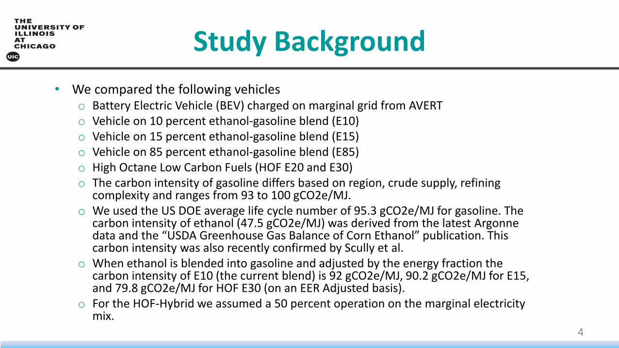
Study Background • We compared the following vehicles

o Battery Electric Vehicle (BEV) charged on marginal grid from AVERT o Vehicle on 10 percent ethanol-gasoline blend (E10) o Vehicle on 15 percent ethanol-gasoline blend (E15) o Vehicle on 85 percent ethanol-gasoline blend (E85) o High Octane Low Carbon Fuels (HOF E20 and E30) o The carbon intensity of gasoline differs based on region, crude supply, refining

complexity and ranges from 93 to 100 gCO2e/MJ. o We used the US DOE average life cycle number of 95.3 gCO2e/MJ for gasoline. The

carbon intensity of ethanol (47.5 gCO2e/MJ) was derived from the latest Argonne data and the “USDA Greenhouse Gas Balance of Corn Ethanol” publication. This carbon intensity was also recently confirmed by Scully et al.

o When ethanol is blended into gasoline and adjusted by the energy fraction the carbon intensity of E10 (the current blend) is 92 gCO2e/MJ, 90.2 gCO2e/MJ for E15, and 79.8 gCO2e/MJ for HOF E30 (on an EER Adjusted basis).

o For the HOF-Hybrid we assumed a 50 percent operation on the marginal electricity mix.

4

Study Background • When calculating the life cycle GHG emission of EVs many

prominent US Government and NGO calculator tools only utilize average U.S. electricity emissions factors or regional, average annual electricity grid emissions factors.

• In reality, however, the large projected addition of EVs to the incumbent grids will constitute a marginal load addition in an environment of generation resource retirements and additions.

• A marginal generating resource is the lowest cost power plant that adapts its power generation capacity in response to a change in power demand.

• As EV populations grow, the long-run marginal generation resource will be the source of power.

5

Electric Load Addition: Generation Dispatch Stack

6

With load increase curve shifts upwards. Tasking more fossil resources and peaking resources Assumes Load Increase across all hours of the day

EPA’s AVoided Emissions and geneRation Tool (AVERT) model

• In the present study we calculated the marginal Electric Vehicle emissions factors for a region using the latest version of EPA’s AVoided Emissions and geneRation Tool (AVERT) model, which was released in September 2020.

• As the user manual of AVERT states: “within each region across the country, system operators decide when, how, and in what order to dispatch generation from each power plant in response to customer demand for electricity in each moment and the variable cost of production at each plant.”

• AVERT analyzes how hourly changes in demand change the output of fossil generators and with that their hourly generation, heat input, and emissions of PM2.5, SO2, NOx, and CO2.

7

Electric Dispatch Regions (AVERT)

8

US Department of Energy EIA states that “if all five reactors close as scheduled, 2021 will set a record for the most annual nuclear capacity retirements ever.” It is widely published that nuclear resources will be mostly replaced by natural gas fired ones. , , https://www.eia.gov/todayinenergy/detail.php?id=46436#:~:text=At%205.1%20GW%2C%20nuclear%20capacity,operating%20U.S.%20nuclear%20generating%20capacity.&text=Each%20of%20these%20plants%20has,combined%20capacity%20is%204.1%20GW

4.1 Gigawatt of Nuclear Retirements Announded on MidAtlantic Grid

Difference: Marginal vs. Average

AVERT Region

Avert 2019 lbs/MWh*

eGrid Region eGRID 2018 lbs/MWh**

eGRID with Transmission Loss

%Diff Marginal to eGrid Avg

Colorado Rocky Mountain

1,904 RMPA 1,171 1,231 55%

Illinois - Chicago

Mid-Atlantic 1,540 RFCW 1,174 1,234 25%

Illinois - Rural

Midwest 1,860 SRMW 1,677 1,763 6%

Indiana Midwest 1,860 RFCW 1,174 1,234 51% Iowa Midwest 1,860 MROW 1,249 1,313 42% Kansas Central 1,800 SPNO 1,172 1,232 46% Kentucky Midwest 1,800 SRTV 1,038 1,091 65% Michigan Midwest 1,860 RFCM 1,321 1,389 34% Minnesota Midwest 1,860 MROW 1,249 1,313 42% Missouri Midwest 1,860 SRMW 1,677 1,763 6% Nebraska Central 1,800 MROW 1,249 1,313 37% North Dakota

Midwest 1,860 MROW 1,249 1,313 42%

Ohio Mid Atlantic 1,540 RFCW 1,174 1,234 25% South Dakota

Midwest 1,800 MROW 1,249 1,313 37%

Wisconsin Midwest 1,860 RFCW,MROWE/MROW

1,420 1,493 25%

*already adjusted for transmission loss **eGrid Output factors not adjusted for transmission loss

9

EPA Published AVERT marginal emission factors for each AVERT region. We compared those marginal factors to EPA’s average eGRID factors (adjusted for transmission loss). EPA eGrid is used in many EV charging calculator tools. Marginal factors for many states are significantly higher than the average emissions factors (red values in table).

Results: Metro Chicago vs. Rural Illinois

10

The light grey area represents the carbon intensity of EVs charged on the local, marginal electricity mix by month. The darker sections of the curve represent an additional penalty assigned to EVs for inefficiencies during winter charging.

Results for Metro Chicago which is connected to the Midwest AVERT* Region.

Rural Illinois which is connected to the Mid-Atlantic AVERT* Region.

Other Examples

11

Coal 104

Summary • EV and ethanol-gasoline blends provide substantial greenhouse gas reductions relative to gasoline-only

vehicles. • High octane fuel vehicles with ethanol and E85 provide very similar GHG savings compared to EVs

(within 5 gCO2e/MJ of each other) for many states. • Ethanol at high blend levels can provide immediate GHG benefits while EV adoption increases. • Long-term, due to the similar GHG savings of EVs and HOF, promoting both technology options towards

the same adoption level across many Midwestern states should double the GHG emissions reductions that can be achieved by any one technology alone.

• Utilities in the Midwest face significant challenges when implementing load shaping and demand side measures to avoid EV charging on both peak load and during marginal coal/natural gas hours.

• EV’s environmental benefits depend largely on electricity charging patterns and load management of the anticipated large vehicle fleet which are unknown today.

• Research into this topic should demand as much attention as direct and indirect land use life cycle emissions received for biofuels during the Renewable Fuels Standard Development.

• This will ensure a level playing field for different technology alternatives and to fairly evaluate options for more effective climate change policy while reducing the risks to the consumer.

12

Utility Preparedness for EVs a Big Unknown

• Request to the research community, transportation policy makers, utilities to fully disclose what it will take to build out the electricity grid to charge all the EVs and when exactly those EVs will charge given the automaker’s large deployment projections.

• When do utilities want large fleets of EVs to charge? o This is not trivial. Optimal charging time will vary by utility and interconnect area. Note that it can likely not be during

peak hours and in many states not during off-peak hours because dirty resources are on the margin. So when then? o If utilities accommodate EVs with load shaping they should detail how expensive load shaping programs will be

especially since people who do not have off-street parking cannot participate easily (there are environmental equity issues here as well).

• Coal retirements are slowing down, nuclear retirements are speeding up (5.1 GW nuclear retirement this year alone). If we replace these resources with natural gas how does affect the carbon intensity of the grid

• When larger scale biofuels deployment was enabled with the RFS a whole field of science sprung up (and highly supported and initiated by NGOs) to try and understand what this would do to land use and international land use change. o We now go as far as measuring adjustments from rice methane emissions in Asia from the land use change assumed to

result from the RFS. o But it seems that when it comes to EVs few of the NGOs are asking the hard questions.

13

Looking Forward and Comparing Cost Specific Adoption Scenario

Modeling Based on “UIC Domestic Biofuels

Emissions Analysis Model” (dBeam)

14

Cost Assumptions

15

• We assumed a capital cost difference to purchase a BEV of $7,500 which is consistent with the current tax credit to encourage BEV adoption over ICE technology

• All future annual cash flows are discounted at 3%. EER for E20: 1.05; EER for E30:1.1 (forward looking)

Annual Consumption and Cost EV Gasoline Baseline

E10 HOF E20 HOF E30

Annual Distance Travelled

13,000 miles

13,000

13,000

13,000 miles Fuel Economy 82.2 mpg equivalent 25.7 26.1 26.3 mpg HOF Fuel Cost Rate 0.143 $/kWh 3 3 3 $/gallon

Annual Fuel Cost

729 $ 1518 1496 1480 $ Maintenance Cost: 0.066 $/mile 0.088 0.088 0.088 $/mile

Annual Maintenance Cost:

858 $

1,144

1,144

1,144 $

Total Annual Operating Cost:

1,587 $

2,662

2,640

2,624 $

Cost per mile:

0.12 $

0.205

0.203

0.202 $

Cases • Adoption of 16 million high octane low carbon fuel vehicles per year from 2026 through 2035 • BEV adoption per Annual Energy Outlook • HOF technologies: E20 from 2026-2030 then upgrade to E30 from 2031-2035

Results: GHG Emissions

• Modeled adoption of 16 million HOF vehicles each year from 2026 through 2035.

• Emissions savings from BEVs in the near future (next 5 years) are relatively modest due to their low adoption.

• The largest emissions savings occur in the HOF Case since HOF technologies can enter the vehicle pool very rapidly in high numbers once approved and achieve significant savings.

16

Emissions Savings Relative to E10 and E0 Baseline

Summary Table: Emissions Savings Scenario: Years

E20 2026-2030 E30 2031-2035

HOF Vehicle Sales (vehicles per year) 16,000,000 Cumulative GHG Savings (tonnes CO2e) Relative to E10 673,665,118 Cumulative GHG Savings (tonnes CO2e) Relative to E0

1,011,761,406

17

• Relative to E10 business as usual the HOF Scenario save between the years 2026

through 2035 a total of 674 million tonnes of GHG emissions. • Relative to E0 the HOF Scenario saves 1 billion tonnes of GHG emissions

Capital and Operating Cost Analysis

• BEVs have lower maintenance and fuel costs than the Baseline Gasoline ICE vehicles. • HOF technologies also result in operating savings relative to Baseline Gasoline due to their higher fuel economy. • BEVs, however, incur higher initial purchase costs which results in an additional capital outlay

18

All cash flows discounted at 3%

19

Putting GHG Savings into Perspective

Latest Argonne Corn Ethanol LCA update shows that between 2005 to 2019 ethanol use is responsible for 544 milllion tonnes CO2e savings This compares to 1 billion tonnes CO2e savings going forward with HOF technologies.

Contact

20

Steffen Mueller, PhD Principal Economist Energy Resources Center The University of Illinois at Chicago 1309 South Halsted Street Chicago, IL 60607 (312) 316-3498 muellers@uic.edu