Evolution  of  Regression  III:  From  OLS  to  GPS™,  MARS®,  CART®,  TreeNet®  and  

RandomForests®  

March 2013 Dan Steinberg

Mikhail Golovnya Salford Systems

Course  Outline

•  Regression Problem – quick overview •  Classical OLS – the starting point •  RIDGE/LASSO/GPS – regularized regression •  MARS® – adaptive non-linear regression

•  CART® Regression tree •  Bagger and Random Forest® CART ensembles •  TreeNet® Stochastic Gradient Boosting •  Hybrid TreeNet/GPS models

Previous Webinars:

Today’s Webinar

2

Boston  Housing  Data  Set •  Concerns the housing values in Boston area •  Harrison, D. and D. Rubinfeld. Hedonic Prices and the

Demand For Clean Air. Journal of Environmental Economics and Management, v5, 81-102 , 1978

•  Combined information from 10 separate governmental and educational sources to produce this data set

•  506 census tracts in City of Boston for the year 1970 o  Goal: study relationship between quality of life variables and property values o  MV median value of owner-occupied homes in tract ($1,000’s) o  CRIM per capita crime rates o  NOX concentration of nitric oxides (pp 10 million) o  AGE percent built before 1940 o  DIS weighted distance to centers of employment o  RM average number of rooms per house o  LSTAT % lower status of the population o  RAD accessibility to radial highways o  CHAS borders Charles River (0/1) o  INDUS percent non-retail business o  TAX property tax rate per $10,000 o  PT pupil teacher ratio

3

Running  Score:  Test  Sample  MSE Method 20%  random Parametric  

Bootstrap Ba6ery  Partition

Regression 27.069 27.97 23.80 MARS  Reg  Splines 14.663 15.91 14.12 GPS  Lasso/  Regularized   21.361 21.11 23.15

4

Regression  Tree •  Decision tree is a nonparametric learning machine with

capability for classification and regression (select methods)

•  Stepwise procedure in which predictors enter the model one at a time

•  In 1975 Jerome H. Friedman labeled the methodology Recursive Partitioning (his first version for binary target)

•  Procedure works by carving a high dimensional data space into a small to moderate set of regions

•  Produce a prediction for each region

5

Simple  Nonparametric  Regression •  Consider a set of predictors which we simplify,

characterizing each as having just two values (low,high) •  Consider all possible combinations of the predictor

values (K predictors allow for 2K possible patterns) •  Attractive nonparametric model: prediction of target

conditional on predictor values is mean target in the region in the training data

6

Simple  Nonparametric  Regression Mean  Y X1 X2 X3 y1 0 0 0 y2 0 0 0 y3 0 0 1 y4 0 0 1 y5 0 1 0 y6 0 1 0 y7 0 1 1 y8 0 1 1

7

3  predictors  allow  for  8  regions  defined  in  terms  of  whether  the  value  of  any  predictor  is  LOW  (0)  or  HIGH(1) Purely  mechanical,  flexible Resolves  many  challenges  such  as  functional  form

Curse  of  Dimensionality •  Curse of dimensionality: 2K very large number

o  K=16 yields 65,536 regions o  K=32 yields 4.3 billion regions

•  We must often work with hundreds of potential predictors and current predictive analytics problems now using thousands if not tens of thousands

8

Tree  Resolution  of  Curse  of    Dimensionality •  Be selective as to which predictors to select •  Reduce the number of predictors used in model •  Define regions with varying numbers of high/low

conditions •  End result is a similarly inspired non-parametric regression •  Make use of vastly fewer regions

•  Never generate more regions than rows of data

9

Growing  the  Tree •  Tree is grown by starting with all training data in root

node •  Look for a rule based on the available predictors to split

database into two parts •  Rules look like (for continuous predictors) •  Xk <= c

Xk > c

•  For regression we look for the rule that most reduces learn sample MSE

•  Search every possible split point (data value for X) •  Search every available predictor

10

Regression  Tree  Out  of  the  box  results,  no  tuning  of  controls

Test  MSE=  17.296

11

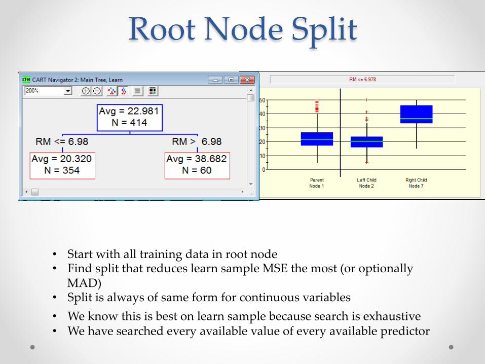
Root  Node  Split

•  Start  with  all  training  data  in  root  node •  Find  split  that  reduces  learn  sample  MSE  the  most  (or  optionally  

MAD) •  Split  is  always  of  same  form  for  continuous  variables •  We  know  this  is  best  on  learn  sample  because  search  is  exhaustive •  We  have  searched  every  available  value  of  every  available  predictor

Next  Split

•  Next  split  could  have  been  on  RM  again  but  LSTAT  performs  beaer •  CART  happens  to  grow  trees  depth  first  (always  looks  for  left  most  node  to  

split  next •  Order  of  spliaing  does  not  maaer.  But  tree  growing  is  myopic.

Third  Split

Order  of  spliaing  nodes  does  not  maaer  as  our  goal  is  to  generate  a  massive  tree Spliaing  will  usually  continue  until  we  run  out  of  data

Grow/Prune  Strategy  Maximal  Tree  (363  nodes)  Test  MSE=22.593  Overfit  fit  but  still  beaer  than  linear  regression

Grow  tree  to  maximum  possible  size:  here  learn  sample  R2  =  1.0 Then  prune  back  to  find  best  performing  sub-­‐‑tree  on  test  sample Maximal  tree  is  almost  certainly  overfit  yet  frequently  offers  decent  performance  on  new  data

Pruning/Back  Stepping •  Back stepping accomplished via weakest-link pruning •  Analogous to backwards stepwise regression: remove split that

harms learn sample performance least •  Defines a set of candidate models each of a different size

16

Access  to  every  tree  in  sequence  of  pruned  trees    from  largest  to  smallest

Several  trees  of  different  sizes  shown.  Allows  choice  of  model  combining  performance,  complexity,  judgment

Test  Error  Displayed  in  Lower  Blue  Curve

Zoom  in

Access  to  every  tree  in  back  pruning  sequence

Click  on  any  point  on  blue  test  sample  performance  curve  to  display  tree  pruned  to  that  size

Green  beam  marks  best  performing  tree

Single Decision Tree •  Key features and strengths of the single CART decision tree

o  Impervious to the scale or coding of predictors. CART uses only rank order information to partition data

o  CART tree is unaffected by order preserving transforms of data

o  Any single split involves only one predictor (in standard mode) meaning that collinearity becomes largely irrelevant

o  Automatic variable selection methodology built-in

o  Missing value handling in CART managed via surrogate splitters (substitute splitters used when primary splitter is missing). A form of local implicit missing value imputation

o  CART is the only learning machine that can handle patterns of missing values not seen in the training data

19

Regression  Tree •  Generally the single regression tree is not expected to

perform outstandingly •  Works by carving a high dimensional data space into

mutually exclusive and collectively exhaustive regions •  Single prediction (mean for the region) is generated for

every region o  Our optimal tree above produces only 9 distinct outputs o  For any input record there are only 9 possible predicted values

•  Linear regression typically produces a unique response for every input record (for rich enough data)

20

Regression  Tree  Representation  of  a  Surface  High  Dimensional  Step  function

Should  be  at  a  disadvantage  relative  to  other  tools.  Can  never  be  smooth. But  always  worth  checking

Regression  Tree  Partial  Dependency  Plot

LSTAT NOX

Use  model  to  simulate  impact  of  a  change  in  predictor Here  we  simulate  separately  for  every  training  data  record  and  then  average For  CART  trees  is  essentially  a  step  function May  only  get  one  “knot”  in  graph  if  variable  appears  only  once  in  tree   See  appendix  to  learn  how  to  get  these  plots

Distribution  of  MV  Within  Node

Learn  &  Test  Within  Node

Repeated  Runs  Different  20%  Test  Samples

100  repetitions  dividing  data  random  into  80%  learn,  20%  test Percentiles:  5th=12.73      95th  MSE=  32.32,  median  20.66

25

Running  Score Method 20%  random Parametric  

Bootstrap Repeated  100   20%  Partitions

Regression 27.069 27.97 23.80 MARS 14.663 15.91 14.12 GPS  Lasso 21.361 21.11 23.15 CART 17.296 17.26 20.66

26

Regression Trees and Ensembles of Trees •  Shortly after the regression tree began to enjoy success in

real world and scientific applications search began for improvements

•  One early idea for improvement was the notion of the committee of experts o  Instead of having just one predictive model generate several models o  Allow the separate models to vote for classification o  Majority rule to arrive at a final classification o  Regression committees just average individual predictions

•  Challenge: How to generate committees (or ensembles) o  Needs to be automatic to be practical o  Too expensive to use competing modeling teams or to allow time develop hand

made alternative models

27

Bagger (Bootstrap Aggregation) •  Breiman introduced the influential “Bagger” in 1996 to solve

the automatic model generation problem •  Intuition: Imagine that we have an unlimited supply of data

o  Draw a random sample from the master data (of good size) •  Sample could be stratified to oversample rare target class

o  Grow a regression tree o  Draw a new, different, random sample from the master data o  Grow a new regression tree o  Process can be continued indefinitely as each draw will result in a different

sample and typically a different (at least slightly) tree o  Combine results into a single prediction for any input data record o  For BINARY classification let the number of YES votes be model score

28

Bootstrap Sampling Details •  Bootstrap resampling is defined as sampling with replacement •  We do not literally extract a record from the original training

set but only copy it •  We then forget that this record was copied into the new

training data set and allow it to be selected again •  Natural to think that since each record has only a very small

chance of being selected, being selected more than once would be a rare event

•  However, about 26% of the original data will be selected more than once in the construction of a standard bootstrap sample (much more than everyday intuition would suggest)

29

OOB: Records Not Selected: About 36.8%

•  OOB “Out of Bag” records •  In a same-size bootstrap sample more than a third of the

original records will not be drawn into new sample •  This is an important artifact of the sample generation process •  Ensures that the bootstrap samples are fairly different from

each other in terms of which records are included •  The shortfall of records is compensated for by drawing extra

copies of the data that is included •  Including a record more than once does not add information

but it gives added weight to that record

•  OOB records can be used for testing. An extreme form of cross-validation

30

Bootstrap Sample Reweighting: An example

•  Probability of being omitted in a single draw is (1 - 1/n) •  Probability of being omitted in all n draws is (1 - 1/n)n •  Limit of series as n goes to infinity is (1/e) = 0.368

o  approximately 36.8% sample excluded 0.0 % of resample o  36.8% sample included once 36.8 % of resample o  18.4% sample included twice thus represent 36.8 % of resample o  6.1% sample included three times ... 18.4 % of resample

o  1.9% sample included four or more times completes sample Example: distribution of weights in a 2,000 record random resample:

0 1 2 3 4 5 6732 749 359 119 32 6 30.366 0.375 0.179 0.06 0.016 0.003 0.002

31

Bagger Mechanism •  Generate a reasonable number of bootstrap samples

o  Breiman started with numbers like 50, 100, 200

•  Grow a standard CART tree on each sample •  Use the unpruned tree to make predictions

o  Pruned trees yield inferior predictive accuracy for the ensemble

•  Simple voting for classification o  Majority rule voting for binary classification o  Plurality rule voting for multi-class classification o  Average predicted target for regression models

•  Will result in a much smoother range of predictions o  Single tree gives same prediction for all records in a terminal node o  In bagger records will have different patterns of terminal node results

•  Each record likely to have a unique score from ensemble

32

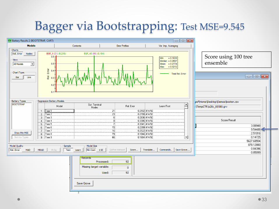
Bagger  via  Bootstrapping:  Test  MSE=9.545

Score  using  100  tree  ensemble

33

Predictions  From  First  6  Trees

First  10  records  of  TEST  partition First  6  Bagger  Trees,  each  tree  grown  to  maximal  size  unpruned No  feedback,  learning,  or  tuning  derived  from  test  partition Predictions  vary  as  each  tree  is  built  on  a  different  bootstrap  sample Bagger  outputs  the  AVERAGE  prediction  for  a  regression  model TEST  MSE=9.545

34

CART  Partial  Dependency  Plot LSTAT NOX

Use  model  to  simulate  impact  of  a  change  in  predictor Here  we  simulate  separately  for  every  training  data  record  and  then  average For  CART  trees  is  essentially  a  step  function May  only  get  one  “knot”  in  graph  if  variable  appears  only  once  in  tree   See  appendix  to  learn  how  to  get  these  plots

Bagger  Partial  Dependency  Plot

LSTAT NOX

Averaging  over  many  trees  allows  for  a  more  complex  dependency Opportunity  for  many  splits  of  a  variable  (100  large  trees) Jaggedness  may  reflect  existence  of  interactions

36

Running  Score Method 20%  random Parametric  

Bootstrap Ba6ery  Partition

Regression 27.069 27.97 23.80 MARS 14.663 15.91 14.12 GPS  Lasso 21.361 21.11 23.15 CART 17.296 17.26 20.66 Bagged  CART  9.545 12,79

37

RandomForests:  Bagger  on  Steroids •  Leo Breiman was frustrated by the fact that the bagger did

not perform better. Convinced there was a better way •  Observed that trees generated bagging across different

bootstrap samples were surprisingly similar •  How to make them more different? •  Bagger induces randomness in how the rows of the data are

used for model construction •  Why not also introduce randomness in how the columns are

used for model construction •  Pick a random subset of predictors as candidate predictors –

a new random subset for every node

•  Breiman was inspired by earlier research that experimented with variations on these ideas

•  Breiman perfected the bagger to make RandomForests

38

RF  Main  Innovation  Counter-­‐‑Intuitive •  Picking splitter at random appears to be a recipe for

poor trees •  Indeed the RF model may not perform so well if the

splitter is chosen completely at random o  At every node choose the variable that splits the node at random o  Better to allow at least some opportunity for optimization by considering

several potential splitters

•  By limiting access to a different subset of predictors at each node we guarantee that trees will be different across the different bootstrap samples

•  Performance of individual trees on holdout data might be inferior to bagger trees but ensemble will do better

39

RF  Model  using  defaults:    Test  MSE=8.286

           RF  Controls

RF  Results

40

Running  Score Method 20%  random Parametric  

Bootstrap Ba6ery  Partition

Regression 27.069 27.97 23.80 MARS 14.663 15.91 14.12 GPS  Lasso 21.361 21.11 23.15 CART 17.296 17.26 20.66 Bagged  CART  9.545 12,79 RF  Defaults  8.286 12.84

41

RF  Core  Parameter:  N  Predictors •  Tuning parameter that can have a substantial impact on

model predictive performance •  K predictors available •  PREDS=1 all splitters chosen completely at random •  Breiman had suggested SQRT(K) and LOG2(K) as good

defaults o  1000 predictors suggests PREDS=32 (SQRT rule) or

PREDS=10 (log2 rule) o  Typically PREDS far below K o  Experimentation is needed o  To obtain honest performance measures, make judgments just on

OOB performance then consult TEST performance

42

Varying  PREDS  Try  every  value  from  1  to  13

Test  Sample  results

OOB  Results At  optimum  OOB  PREDS=6  Test  MSE=8.002

Purely-­‐‑  at-­‐‑random  RF  yields  inferior  results  but  still  impressive  (Test  MSE=11.15)

43

Running  Score Method 20%  random Parametric  

Bootstrap Ba6ery  Partition

Regression 27.069 27.97 23.80 MARS 14.663 15.91 14.12 GPS  Lasso 21.361 21.11 23.15 CART 17.296 17.26 20.66 Bagged  CART  9.545 12.79 RF  Defaults  8.286 12.84 RF  PREDS=6  8.002 12.05

44

RandomForests  Strengths •  RandomForests can be used for

o  Classification (binary or multi-class classification) o  Regression (prediction of a continuous target) o  Clustering/Density estimation

•  Robust behavior relatively insensitive to dirty data •  Easy to use with few control parameters •  Graphical displays of key model insights •  RandomForests can be effectively used with wide data

sets o  Possibly many more columns than rows o  High speed even with millions of predictors

•  Naturally parallelizable as every tree grown independently

•  Retains advantages offered by most regression trees •  Very strong variable (predictor) selection

45

Stochastic Gradient Boosting (TreeNet ) •  SGB is a revolutionary data mining methodology first

introduced by Jerome H. Friedman in 1999 •  Seminal paper defining SGB released in 2001

o  Google scholar reports more than 1600 references to this paper and a further 3300 references to a companion paper

•  Extended further by Friedman in major papers in 2004 and 2008 (Model compression and rule extraction)

•  Ongoing development and refinement by Salford Systems o  Latest version released 2013 as part of SPM 7.0

•  TreeNet/Gradient boosting has emerged as one of the most used learning machines and has been successfully applied across many industries

•  Friedman’s proprietary code in TreeNet

46

TreeNet Gradient Boosting Process •  Begin with one very small tree as initial model

o  Could be as small as ONE split generating 2 terminal nodes

o  Default model will have 4-6 terminal nodes

o  Final output is a predicted target (regression) or predicted probability

o  First tree is an intentionally “weak” model

•  Compute “residuals” for this simple model (prediction error) for every record in data (even for classification model)

•  Grow second small tree to predict the residuals from first tree

•  New model is now:

Tree1 + Tree2

•  Compute residuals from this new 2-tree model and grow 3rd tree to predict revised residuals

47

Trees incrementally revise predictions

First tree grown on original target. Intentionally “weak” model

2nd tree grown on residuals from first. Predictions made to improve first tree

3rd tree grown on residuals from model consisting of first two trees

+ +

Tree 1 Tree 2 Tree 3

Every tree produces at least one positive and at least one negative node. Red reflects a relatively large positive and deep blue reflects a relatively negative node. Total “score” for a given record is obtained by finding relevant terminal node in every tree in model and summing across all trees

48

Gradient  Boosting    Methodology:  Key  points

•  Trees are usually kept small (2-6 nodes common) o  However, should experiment with larger trees (12, 20, 30

nodes) o  Sometimes larger trees are surprisingly good

•  Updates are small (downweighted). Update factors can be as small as .01, .001, .0001. o  Do not accept the full learning of a tree (small step size, also GPS

style) o  Larger trees should be coupled with slower learn rates

•  Use random subsets of the training data in each cycle. Never train on all the training data in any one cycle o  Typical is to use a random half of the learn data to grow each tree

49

Gradient  Boosting  Contrast  With  Single  Tree •  Every cycle of learning begins with entire training data

set •  Equivalent to going back to the root node with respect

to availability of data o  Single tree drills progressively deeper into data, working

with progressively smaller subsamples o  Single tree cannot share information across nodes (local) o  Deep in tree sample sizes may not support discovery of

important effects which in fact are common across many of the deeper nodes (broader, even global structure)

•  Gradient boosting rapidly returns to root node with the construction of a new tree – target variable has changed however o  Target is set of residuals from previous iteration of model

50

TreeNet  Gradient  Boosting  Model  Setup

Differ from defaults only in selecting Least Squares Loss and TREES=1000 Best TreeNet results frequently require thousands of trees

51

Gradient  Boosting  Results  (LOSS=LS)

Progress of model as trees are added Best MSE and best MAD typically occur with different sized models (N Trees) Essentially default settings yields Test MSE= 7.417 (bit better yet allowing 1200 trees)

52

Running  Score Method 20%  random Parametric  

Bootstrap Ba6ery  Partition

Regression 27.069 27.97 23.80 MARS 14.663 15.91 14.12 GPS  Lasso 21.361 21.11 23.15 CART 17.296 17.26 20.66 Bagged  CART  9.545 12,79 RF  Defaults  8.286 12.84 RF  PREDS=6  8.002 12.05 TreeNet  Defaults 7.417 8.67 11.02

Using cross-validation on learn partition to determine optimal number of trees and then scoring the test partition with that model: TreeNet MSE=8.523

53

Tuning  Gradient  Boosting  Regression

•  Huber loss function uses squared error for the smaller errors •  For larger errors incremental loss is based on absolute error •  Robust form of regression less sensitive to outliers

54

Vary  HUBER  Threshold:  Best  MSE=6.71

Vary threshold where we switch from squared errors to absolute errors Optimum when the 5% largest errors are not squared in loss computation

Yields best MSE on test data. Sometimes LAD yields best test sample MSE.

55

Gradient  Boosting  Partial  Dependency  Plots

56

LSTAT NOX

Running  Score Method 20%  random Parametric  

Bootstrap Ba6ery  Partition

Regression 27.069 27.97 23.80 MARS 14.663 15.91 14.12 GPS  Lasso 21.361 21.11 23.15 CART 17.296 17.26 20.66 Bagged  CART  9.545 12,79 RF  Defaults  8.286 12.84 RF  PREDS=6  8.002 12.05 TreeNet  Defaults 7.417 8.67 11.02 TreeNet  Huber 6.682 7.86 11.46 TN  Additive 9.897 10.48

If we had used cross-validation to determine the optimal number of trees and then used those to score test partition the TreeNet Default model MSE=8.523

57

Interactions •  When the impact of the change in a predictor Xi

depends on the value of another predictor Xj •  Classical statistical models usually start with creating a

new feature defined as the product Xi*Xj •  Extraordinarily difficult to discover, refine, select

interactions into classical models •  Trees generate interactions naturally (perhaps too many

and too readily) •  Technically there is an an interaction between Xi and Xj

if the two predictors appear on the same branch of a tree

•  Still need to check to see if in simulations there really is any material dependency that qualifies as an interaction

58

Preventing  An  Interaction •  Friedman suggested that one can develop models

without interactions by just growing 2-node trees •  If this technique is used one must compensate for the

restricted learning allowed in each tree by growing many more trees

•  Preventing interactions in the TreeNet model substantially increases the test sample MSE to 9.897

59

Interaction  Detection  with  TreeNet •  TreeNet offers diagnostics and formal tests for the

existence of interactions and their strengths •  Build a model without interactions (for example, limiting

depth of the tree to one split only) •  Compare results with a more flexible model (trees

allowed to grow deeper) •  TreeNet offers reports based on these comparisons

60

TreeNet  Interaction  Strength  Measures  LOSS=LS

•  ====================!•  TreeNet Interactions!•  ====================!

•  Whole Variable Interactions!•  Measure Predictor!•  ------------------------------!•  18.18831 LSTAT!•  8.99670 DIS!•  7.83481 RM!

•  6.67131 NOX!•  6.18011 CRIM!•  4.75381 AGE!•  4.08043 B!•  3.82925 PT!•  2.39673 TAX!

•  1.52854 INDUS!•  0.95982 RAD!•  0.82921 CHAS!•  0.27512 ZN!

Interaction strength is a measure of the difference between predictions generated by a flexible and additive model For a specific 2-way interaction the differences are measured over the joint range of the pair of predictors in question Statistical tests are required to eliminate “spurious” interactions

61

Top  Ranked  2-­‐‑way  interactions

62

Parametric  Bootstrap  Evaluate  True  Strength  of  Interactions

Blue bar: Mean difference in strength measure (flexible – additve) Red bar: Standard Deviation of strength measure (in additive model)

63

Hybrid  Models:  ISLE •  There are many styles of hybrid model •  We focus on just one: Importance Sampled Learning

Ensembles •  We start with an ensemble of trees and treat each of

them as a new feature o  Every tree transforms the one or more predictors into a single output o  Create a data set in which every tree of the ensemble is a “variable” o  Could be a very large number of such new features (thousands)

•  Now use regularized regression to select and reweight the trees o  Could yield a model with a much smaller set of trees

64

Example  of  an  important  interaction  

•  Slope reversal due to interaction

Note  that  the  dominant  paaern  is  downward  sloping But  a  key  segment  defined  by  the  3rd  variable  is  upward  sloping

65

What’s  Next •  Hands-on session, part IV •  Live walk through examples using

o  Regression trees o  Ensemble models (Bagger) o  Random Forests o  TreeNet Stochastic Gradient Boosting o  TreeNet/GPS Hybrid models

66

Some other Variations of Bagger •  Decision Forest: Keep training data set fixed but randomly select

which predictors to use (a random half of all predictors for any tree) o  Grow many trees and then combine via voting or averaging

•  Bagged Decision Forest: Randomize both over the training records and the allowed predictors o  Each data set is a different bootstrap sample o  Each predictor set is a different random half of available predictors

•  For binary classification problem vary priors systematically over a broad range o  Data set remains unchanged o  Important tree growing parameter is changed systematically

•  Random Splitter selection from top K best predictors (Dieterrich) •  Wagging: Exponential distribution assigns non-zero weights to all records

o  Webb and Zheng (2004) IEEE Transactions on Knowledge and Data Engineering o  Inferior to bagging but designed for systems that must include all records in every tree

67

ISLE  Ensemble  Compression

68

GPS  regularized  regression  progress  in  dashed  line TreeNet  Gradient  Boosting  ensemble  solid  line In  this  example  negligible  improvement  and  slight  compression

Strength of Interaction Measurement: Friedman’s measure

•  From the TreeNet model extract the function (or smooth) Y(xi, xj | Z) (1) We extract the smooth by using our actual training data and setting Xi=a, Xj=b and then averaging predicted Y over all records. We then vary the preset values of a and b to extract the model generated surface

•  Now repeat the process for the single dependencies Y(xi | xj, Z) (2) Y(xj | xi, Z) (3)

•  Compare the predictions derived from (1) with those derived from (2) and (3) across an appropriate region of the (xi, xj) space

•  Construct a measure of the difference between the two 3D surfaces (1) and (2)+(3)

69

Jerome Friedman •  Friedman is one of the most influential researchers in data

mining o  Studied Physics at UC Berkeley o  Professor in Statistics at Stanford since 1975

•  Co-author of the CART decision tree in 1984 (Classification and Regression trees (with Jerome Friedman, Richard Olshen, and Charles Stone)

•  Creator of MARS regression splines, PRIM rule discovery, ISLE ensemble compression, GPS regularized regression, Rule Learning Ensembles

•  Series of many influential machine learning papers spanning 40 years

70

Salford  Predictive  Modeler  SPM •  Download a current version from our website

http://www.salford-systems.com

•  Version will run without a license key for 10-days

•  Request a license key from unlock@salford-systems.com

•  Request configuration to meet your needs o  Data handling capacity o  Data mining engines made available

71