evolution of database emerging to sybase adaptive server...
TRANSCRIPT
International Journal of Computer Applications (0975 – 8887)
Volume 35– No.1, December 2011
37
Evolution of Database Emerging to Sybase Adaptive Server Enterprise and Ensuring Better Server Performance
Tuning and Query Optimization
Mohammad Ghulam Ali Fellow (BCS), UK, Life Member IACSIT (Singapore), IAENG (Hong Kong)
System Engineer Academic Post Graduate Studies & Research
Indian Institute of Technology, Kharagpur Kharagpur - 721 302 West Bengal, India
ABSTRACT Evolution of the database is emerging to a robust Sybase
Adaptive Server Enterprise Database System. Key issue in the
Sybase Database System is to obtain better server performance
by tuning the server and optimizing the query processing. The
server performance tuning and query optimization are two main
issues to gain high throughput and less or fast response time. In
this paper we have considered well two issues and explained
how to gain better server performance by tuning the server and
optimizing the query processing. We are also illustrating
solutions to some situations normally occurs related to this two
issues in this paper. This paper will introduce the reader to the
most basic concepts of server performance tuning, query
processing and optimization of query processing. We hope this
paper will provide an adequate support to Database
Administrator(s) (DBAs) who are working on Sybase and
researchers who are working on Database Server performance
tuning and query optimization. We have discussed in brief in the
introduction section of this paper about the evolution of the
database emerging to SYBASE ASE version under different
operating system environments.
General Terms Database Server Performance Tuning and Query Optimization
Keywords Database, Database Management System, Relational Database
Management System, Performance Tuning, Query Processing,
Query Optimization.
1. INTRODUCTION Keeping in mind the progress in communication and database
technologies (concurrency, consistency and reliability) has
increased the data processing potential. Various protocols and
algorithms are proposed and implemented for network
reliability, concurrency, atomicity, consistency, recovery,
replication, query processing and query optimization. Any
application or information system is mainly built from four
components and that are user interface that handles information
on screen, application program logic that handles the processing
and information, integrity logic that governs how information is
processed and kept accurate within an
organization and finally data access that is the method of storing
and retrieving data from a physical device. We now want an
optimal performance of Database Server and fast query
processing in any Information System proposed and that will
access to the database. We want an efficient and quick retrieval
of information for any kind of decision supports. For this, server
performance in general and optimization in particular are two
main issues. We have considered Sybase as a robust database
system in this paper. Recent versions of Sybase ASE have
brought a great deal of change in the realm of optimization.
Sybase ASE is known for its reliability, robustness, and
availability, supports large applications with hundreds and
thousands of concurrent users, and well-suited for customized
transactional applications. This paper has addressed two issues
(Server Performance Tuning and Query Optimization) well
however this two issues are big. We can also say poor SQL
statement performance and high CPU usage on our Sybase ASE
server almost always indicates the need for performance tuning.
This paper has an introduction section including evolution of
database in brief and an introduction to Sybase SQL Server and
Sybase ASE including Sybase ASE overview, performance
tuning section and query processing and optimization of query
processing section. We are also illustrating some solutions to
situations normally occurs during server run time related to the
server performance tuning and query optimization in a separate
section, and finally we conclude the paper.
1.1 Evolution of Database We first discuss few about evolution of database. We first
explain about Data Hierarchy. A bit binary digits, A byte
represents a character (basic building unit of data), A field (a
logical grouping of characters), A record (a logical grouping of
related fields), A file (a logical grouping of related records), A
database (a logical grouping of related files).
In general database is a collection of organized and related
records. The Database Management System (DBMS) provides a
systematic and organized way of storing data, managing data
and retrieving data from a collection of logically related
information stored in a database. Database Management System
(DBMS) did not come into industries until 1960‘s. First DBMS
appeared right before 1970. All database systems are evolved
from a file system.

International Journal of Computer Applications (0975 – 8887)
Volume 35– No.1, December 2011
38
Originally, databases were flat. This means that the information
was stored in one long text file, called a tab delimited file. Each
entry in the tab delimited file is separated by a special character,
such as a vertical bar (|). Each entry contains multiple pieces of
data in the form of information about a particular object or
person grouped together as a record. The text file makes it
difficult to search for specific information or to create reports
that include only certain fields from each record.
The File Management System also called as FMS in short is one
in which all data is stored on a single large file.
Researchers in database field, however, found the data has its
value, and models based only on data be introduced to improve
the reliability, security, efficiency of the access and to come out
from the drawbacks of the file based systems and that leads to
the introduction of the Hierarchical Data Model and the
Hierarchical Database Management System.
Data models provide a way in which the stored data is organized
as specified structure or relation for quick access and efficient
management. Data models formally define data elements and
relationships among data elements for a domain of interest.
A data model instance may be one of three kinds according to
ANSI/SPARC (American National Standards Institute,
Standards Planning and Requirements Committee) in 1975. 1)
Logical Schema/Conceptual Schema/Conceptual Level, 2)
Physical Schema/Internal Level and 3) External
Schema/External Level.
We discuss in brief about different generation data models and
database management systems.
1.1.1. 1st Generation Data Model and Database
Management System (DBMS) Hierarchical and Network Data Models are considered under 1st
Generation Data Model.
Hierarchical Data Model and Hierarchical Database
Management System existed from mid 1960- early 1980. The
previous system FMS drawback of accessing records and sorting
records which took a long time was removed in this by the
introduction of parent-child relationship between records in the
database. Each parent item can have multiple children, but each
chilled item can have one and only one parent. Thus
relationships in the hierarchical database either one-to-one or
one-to-many. Many-to-Many relationships are not allowed. The
origin of the data is called the root from which several branches
have data at different levels and the last level is called the leaf.
Hierarchical databases are generally large databases with large
amounts of data. The hierarchical data model organizes data in a
tree structure or as some call it, an "inverted" tree. There is a
hierarchy of parent and child data segments. Prominent
hierarchical database model was IBM‘s first DBMS called IMS.
In mid 1960s Rockwell partner with IBM created information
Management System (IMS), IMS DB/DC leads to the
mainframe database market in 70‘s and early 80‘s.
In order to avoid all drawbacks of the Hierarchical Data Model,
a next data model and database management system took its
origin which is called as the Network Model and Network
Database Management System. Network Data Model and
Network Database Management System was introduced in 1969
almost the exact opposite of the Hierarchical Data Model. In this
the main concept of many-many relationships got introduced.
Network Model eliminates redundancy but at the expense of
more complicated relationships. This model can be better than
hierarchical model for some kinds of data storage tasks, but
worse for others. Neither one is consistently superior to other.
1.1.2. 2nd Generation Data Model (Relational
Model) and Relational Database Management
System (RDBMS) – 1970 Relational Data Model is considered under 2nd Generation Data
Model.
In order to overcome all the drawbacks of the previous data
models and database management systems the Relational Data
Model and the Relational Database Management System got
introduced in 1970, in which data get organized as tables and
each record forms a row with many fields or attributes in it.
Relationships between tables are also formed in this system. A
tuple or row contains all the data of a single instance of the
table. In the relational model, every tuple must have a unique
identification or key based on the data that uniquely identifies
each tuple in the relation. Often, keys are used to join data from
two or more relations based on matching identification. The
relational model also includes concepts such as foreign keys,
which are primary keys in one relation that are kept in another
relation to allow for the joining of data.
In 1970 Dr. Edgar F. Codd at IBM published the relational
Model. A relational database is a collection of relations or
tables. By definition, a relation becomes a set of tuples having
the same attributes. Operations, which can be performed on the
relations are select, project and join. The join operation
combines relations, the select queries are used for data retrieval
and the project operation identifies attributes. Similar to other
database models, even relational databases support the insert,
delete and update operations.
Basically, relational databases are based on relational set theory.
Normalization is a vital component of relational model of the
databases. Relational operations which are supported by the
relational databases work best with normalized tables. A
relational database supports relational algebra, relational
calculus, consequently supporting the relational operations of
the set theory. Apart from mathematical set operations namely,
union, intersection, difference and Cartesian product, relational
databases also support select, project, relational join and division
operations. These operations are unique to relational databases.
Relational databases support an important concept of dynamic
views. In a relational database, a view is not a part of the
physical schema, it is dynamic. Hence changing the data in a
table alters the data depicted by the view. Views can subset data,
join and simplify multiple relations, dynamically hide the
complexity in the data and reduce the data storage requirements.
Relational databases use Structured Query Language (SQL)
which is invented by IBM in 1970 and SQL is a declarative
language, which is an easy and human-readable language. SQL
instructions are in the form of plain instructions, which can be
put to the database for implementation. Most of the database
vendors support the SQL standard.
Relational databases have an excellent security. A relational
database supports access permissions, which allow the database

International Journal of Computer Applications (0975 – 8887)
Volume 35– No.1, December 2011
39
administrator to implement need-based permissions to the access
of the data in database tables. Relational databases support the
concept of users and user rights, thus meeting the security needs
of databases. Relations are associated with privileges like create
privilege, grant privilege, select, insert and delete privileges,
which authorize different users for corresponding operations on
the database.
The other important advantages of relational databases include
their performance, power, and support to new hardware
technologies as also flexibility and a capacity to meet all types
of data needs. Relational databases are scalable and provide
support for the implementation of distributed systems.
Owing to their advantages and application in the operations of
data storage and retrieval of the modern times, relational
databases have revolutionized database management systems.
SYBASE is an example of relational database. However,
SYABASE ASE has also objected oriented features.
In relational Model, values are atomic (value as one that cannot
be decomposed into smaller pieces by the DBMS such as Bank
Account No., Employee Code etc. or Columns in a relational
table are not repeating group or arrays), each row is unique,
column values are of the same kind, the sequence of columns is
insignificant (ordering of the columns in the relational table has
no meaning. Columns can be retrieved in any order and in
various sequences. The benefit of this property is that it enables
many users to share the same table without concern of how the
table is organized. It also permits the physical structure of the
database to change without affecting the relational tables), the
sequence of rows is insignificant (the main benefit is that the
rows of a relational table can be retrieved in different order and
sequences. Adding information to a relational table is simplified
and does not affect existing queries), each column has unique
name, certain fields may be designed as keys which means that
searches for specific values of that field will use indexing to
speed up them.
The RDBMS allows for data independence, this helps to provide
a sharp and clear boundary between the logical and physical
aspects of database management.
The RDBMS provides simplicity, this provides a more simple
structure than those that were being before it. A simple structure
that is easy to communicate to users and programmers and a
wide variety of users in an enterprise can interact with a simple
model.
The RDBMS has good theoretical background, this means that it
provides a theoretical background for database management
field.
1.1.3. 3rd Generation Data Model and Database
Management System (DBMS) ER-Model and Semantic Data Model are considered under 3rd
Generation Data Model.
In 1976, six year after Dr. Codd published the relational Model,
Dr. Peter Chen published a paper in the ACM Transaction on
Database Systems, introducing the Entity Relationship Model
(ER Model). An ER Model is intended as a description of real-
world entities. The ER data model views the real world as a set
of basic objects (entities) and relationships among these objects
(Entities, relationships, and attributes). It is intended primarily
for the DB design process by allowing the specification of an
enterprise scheme. This represents the overall logical structure
of the database. Although, it is constructed in such a way as to
allow easy translation to the relational model. The ER diagram
represents the conceptual level of database design. A relational
schema is at the logical level of database design. ER model is
not supported directly by any DBMS. It needs to be translated
into a model that is supported by DBMSs. The entity-
relationship model (or ER model) is a way of graphically
representing the logical relationships of entities (or objects) in
order to create a database. Any ER diagram has an equivalent
relational table, and any relational table has an equivalent ER
diagram.
Semantic Data Model was developed by M. Hammer and D.
McLeod in 1981. The Semantic Data Model (SDM), like other
data models, is a way of structuring data to represent it in a
logical way. SDM differs from other data models, however, in
that it focuses on providing more meaning of the data itself,
rather than solely or primarily on the relationships and attributes
of the data.
SDM provides a high-level understanding of the data by
abstracting it further away from the physical aspects of data
storage.
The semantic data model (SDM) has been designed as a natural
application modeling mechanism that can capture and express
the structure of an application environment. It can serve as a
formal specification and documentation mechanism for a data
base, can support a variety of powerful user interface facilities,
and can be used as a tool in the data base design process.
Object-Oriented Data Model (OODM) and Object Relational
Data Model (ORDM) are considered under Semantic Data
Model.
Object-Oriented Data Model and Object-Oriented Database
Management System (OODBMS) - (early 1980s and 1990s).
Research in the field of databases has resulted in the emergence
of new approaches such as the object-oriented data model and
Object-Oriented Database Management System, which
overcome the limitation of earlier models.
Object-oriented model has adopted many features that were
developed for object oriented programming languages. These
include objects, inheritance (the inheritance feature allows new
classes to be derived from existing ones. The derived classes
inherit the attributes and methods of the parent class. They may
also refine the methods of the parent class and add new methods.
The parent class is a generalization of the child classes and the
child classes are specializations of the parent class),
polymorphism (a mechanism associating one interface with
multiple code implementations) and encapsulation (the
association of data with the code that manipulates that data, by
storing both components together in the database).
Object-Oriented features mainly are Complex objects, object
identity, encapsulation, classes, inheritance, overriding,
overloading, late binding, computational completeness,
extensibility.
Object Database features are mainly persistence, performance,
concurrency, reliability, and declarative queries.
We do not discuss in details here about OODM.

International Journal of Computer Applications (0975 – 8887)
Volume 35– No.1, December 2011
40
Object-Relational Data Model and Object Relational Database
Management System (ORDBMS). The object-relational model
is designed to provide a relational database management that
allows developers to integrate databases with their data types
and methods. It is essentially a relational model that allows users
to integrate object-oriented features into it. The primary function
of this new object-relational model is to more power, greater
flexibility, better performance, and greater data integrity then
those that came before it.
The ORDBMS provides an addition of new and extensive object
storage capabilities to the relational models at the center of the
more modern information systems of today. These services
assimilate the management of conventional fielded data, more
complex objects such as a time-series or more detailed
geospatial data (such as imagery, maps, and vector data) and
varied dualistic media (such as audio, video, images, and
applets). This can be done due to the model working to
summarize methods with data structures, the ORDBMS server
can implement complex analytical data and data management
operations to explore and change multimedia and other more
complex objects.
It can be said that the object relational model is an evolutionary
technology, this approach has taken on the robust transaction
and performance management aspects of its predecessors.
Database developers can now work with somewhat familiar
tabular structures and data definition but with more power and
capabilities.
Object-relational models allow users to define data types,
function, and also operators. As a direct result of this the
functionality and performance of this model are optimized. The
massive scalability of the object-relational model is its most
notable advantage, and it can be seen at work in many of today‘s
vendor programs.
In ORDBMS, SQL-3 is supported. SQL3 is a superset of
SQL/92. SQL3 supports all of the constructs supported by that
standard, as well as adding new ones of its own such as
Extended Base Types, Row Types, User-Defined Types, User-
Defined Routines, Sub-Types and Super-Types, Sub-Tables and
Super-Tables, Reference Types and Object Identity, Collection
Types.
1.1.4. 4th Generation DBMS 4th Generation DBMS is also based on Object-Oriented Data
Model has come into an existence. VERSANT Database is an
example of 4th Generation Database.
Each of these models modeled the data and the relationship
between the data in different ways. Each of the models
encountered some limitations in being able to represent the data
which resulted in other models to compensate for the limitations.
1.2 Sybase (10/11) SQL Server and
Sybase Adaptive Server Enterprise (ASE) Sybase first began to design its relational database management
system in 1984. Sybase Adaptive Server Enterprise (i.e., the
product formerly known as the Sybase SQL Server) became the
leading RDBMS product for high performance transaction
processing supporting large numbers of client application
connections on relatively small, inexpensive hardware. To be
successful in this demanding area, Sybase focused heavily to
optimize and streamline all the layers of database engine for
transaction processing workloads. While this focus turned out to
be the asset that catapulted Sybase to a dominant position in
high end OLTP applications during the 1990's, it increasingly
became a liability in some environments as application
workloads have changed and hardware performance has
increased [12].
Sybase SQL Server is unique among the most popular
Relational Database Management System (RDBMS) products in
that it was planned and designed to operate a client-server
architecture. Sybase Inc., built SQL Server with the network in
mind. Each client process establishes a connection to SQL
Server over the network. Information is sent from client to
server and back again over the network, using standard
Application Programming Interfaces (APIs) [1].
The architecture of SYBASE SQL Server enables developers to
create robust, production-level client-server applications. A
basic understanding of the components of that architecture will
aid developers to create optimally performing applications.
Nowadays the Sybase Data Server is known as Adaptive Server
Enterprise or ASE (to distinguish it from other Sybase database
products like Sybase IQ). Previously it was known as Sybase
SQL Server. The basic unit of storage in ASE is data page. A
data page is the minimum amount of data transferred to and
from disk to the cache. The supported page sizes for ASE are
2K, 4K, 8K and 16K [6].
Version 15.5 of Sybase ASE provides in-memory database
(IMDB) capabilities designed to deliver low response time and
high throughput for mission-critical system. More specifically,
IMDB tends to deliver better performance for write-intensive
workloads [32].
1.2.1 Classification of DBMS Software Architecture
and Sybase Architecture Single Process
A product is designed to use a single-process architecture single
thread requests through the DBMS. This can produce
bottlenecks in a multi-user environment. Single process
architectures are typical for single-user workstation DBMS
products.
Multi-Process
A product is designed to use a multi-process architecture creates
new processes to handle each new request. Quick exhaustion of
system resources (such as memory) can occur as more processes
are initiated. Many multi-user DBMS products are multi-process
architecture.
Single Process, Multi-thread Architecture (SYBASE)
Single Process, multi-thread architecture, employing multiple
threads within a single process to service multiple users. Only
one process will ever run on the server regardless of how many
clients are connected [1].
International Journal of Computer Applications (0975 – 8887)
Volume 35– No.1, December 2011
41
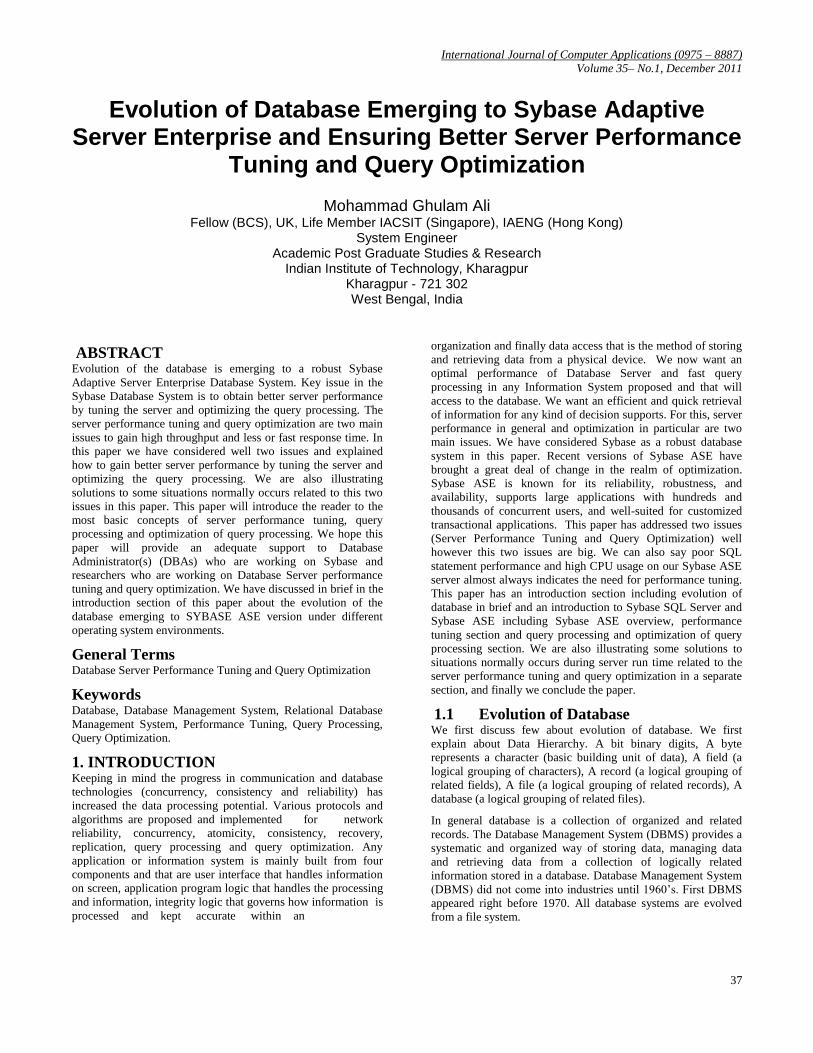
Figure - 1 SYBASE ASE Architecture
Sybase ASE runs as an application on top of an operating
system and depends solely on the services exported by the
operating system to function. It uses operating system services
for process creation and manipulation; device and file
processing; shared memory for interprocess communication.
ASE uses its own thread package for creating, managing, and
scheduling tasks inside Sybase ASE engines for running SQL
Queries and for System tasks like checkpoint, network handler,
house keeper etc. [29]. Figure – 1 illustrates the architecture of
the SYBASE ASE. We do not go in details on this issue here.
We refer to SYBASE manual.
1.2.2. Sybase ASE Overview We discuss few about Sybase ASE overview [5]. For details
please refer to Sybase Manual.
1.2.2.1 The Sybase Server A Sybase database server consists of A) two processes, data
server and backup server. Besides there are Monitor Server, XP
Server and Adaptive Server Utilities. Data Server or Adaptive
Server maintains overall operations of the system databases and
user databases. Backup Server is an open server-based
application that manages all databases backup (dump) and
restore (load) operations for Adaptive Server. Monitor Server is
an open server application that obtains performance statistics on
Adaptive Server makes those statistics available to monitors
Monitor Historical Servers and application build with Monitor
Client Library. XP Server is an open server application that
manages and executes extended stored procedures from within
Adaptive Server. B) devices which house the databases; one
database (master) contains system and configuration data. When
we install Sybase, default databases are [master (6MB), tempdb
(3 MB), sybsystemdb (2 MB), model (2 MB)], and
sybsystemprocs (120 MB). master database controls the
operation of Adaptive Server as whole and stores information
about all users, users databases, devices, objects, and system
table entries as we have discussed earlier too. The master
database is contained entirely on the master device and cannot
be expanded onto any other device. model database provides a
template for new user databases. The model database contains
required system tables, which are copied into a new user
database with the create database command. tempdb is a work
area for Adaptive Server, each time Adaptive Server is started,
the tempdb database is created and built from the model
database. sybsystempdb stores information about transaction in
progress, and which is also used during recovery.
sybsystemprocs database contains most of the Sybase-supplied
System Stored Procedures. System Procedures are collection of
SQL statements and flow-of-control statements that perform
system tasks. Optional databases are sybsecurity for the
auditing. The pubs2 and pubs3 databases are sample databases
provided as learning tool for Adaptive Server. sybsyntax
database contains syntax help for Transact-SQL commands,
Sybase system procedures, dbccdb database stores the result of
dbcc when dbcc checkstorage or dbcc check verifying are used,

International Journal of Computer Applications (0975 – 8887)
Volume 35– No.1, December 2011
42
interpubs database contains French and German data, inetpubs
contains Japanese data. Adaptive Server utilities and open client
routines. C) a configuration file which contains the server
attributes. We do not discuss in details about these here. Please
refer to Sybase Manual.
1.2.2.2. Memory Model The Sybase memory model consists of A) the program area,
which is where the data server executable is stored; B) the data
cache, stores recently fetched pages from the database device;
C) the stored procedure cache, which contains optimized SQL
calls. The Sybase data server runs as a single process within the
operating system as we have discussed earlier; when multiple
users are connected to the database, only one process is
managed by the OS. Each Sybase database connection requires
40-60k of memory. The "total memory" configuration parameter
determines the amount of memory allocated to the server. This
memory is taken immediately upon startup, and does not
increase.
1.2.2.3. Transaction Processing Transactions are written to the data cache, where they advance
to the transaction log, and database device. When a rollback
occurs, pages are discarded from the data cache. The transaction
logs are used to restore data in event of a hardware failure. A
checkpoint operation flushes all updated (committed) memory
pages to their respective tables. Transaction logging is required
for all databases; only image (blob) fields may be exempt.
During an update transaction, the data page(s) containing the
row(s) are locked. This will cause contention if the transaction is
not efficiently written. Record locking can be turned on in
certain cases, but this requires sizing the table structure with
respect to the page size.
The transaction logging subsystem is one of the most critical
components of a database server. To be able to accomplish the
goal of providing recoverability of databases, transactions write
log records to persistent storage. Since a number of such log
record writes is directly dependent on the number of executing
transactions, the logging system can potentially become a
bottleneck in high throughput OLTP environments. All the users
working on a particular database share the log; thus, to
guarantee high performance of the application, it is essential for
the DBA to monitor and configure the log to provide for best
throughput and response time of the application. Out-of-the-box,
Adaptive Server Enterprise (ASE) already provides a high
performance logging subsystem that scales to thousands of users
and very large database (VLDB) environments. ASE also
provides options for the DBA to customize the logging
subsystem to satisfy their unique environments for best
throughput and response times [14].
1.2.2.4. Backup Procedures A "dump database" operation can be performed when the
database is on-line or offline. Subsequent "dump transaction"
commands need to be issued during the day, to ensure
acceptable recovery windows.
1.2.2.5. Recovery Procedures A "load database" command loads the designated database with
the named dump file. Subsequent "load transaction" commands
can then be issued to load multiple transaction dump files.
1.2.2.6. Security and Account Setup The initial login shipped with Sybase is "sa" (System
Administrator). This login has the role "sa_role" which is the
super-user, in Sybase terms. User logins are added at the server
level, and then granted access to each database, as needed.
Within each database, access to tables can be granted per
application requirements. A user can also be aliased as "dbo",
which automatically grants them all rights within a database.
1.2.2.7. Database Creation User databases are initialized with the "create database"
command. In practical Sybase can maintain 100 different
databases in one box. Tables are created within each database;
users refer to tables by using
databasename.ownername.tablename. When we first create a
database, Adaptive Server creates three segments in the database
(System Segment, Log Segment and Default Segment). A
typical Sybase database will consist of six segments spread
across various devices (non-SAN environment). Maximum
database size may be 8 Tera Bytes. Maximum size of the
database devices may be 32 Giga Bytes. We can create
maximum number of database devices per server is 256. We can
create maximum number of segments per database is 31.
1.2.2.8. Data Types Supported data types include integer, decimal, float, money,
char, varchar, datetime, image, and text data types.
1.2.2.9. Storage Concepts Tables are stored in segments; a segment is an area within a
device, with a name and a size, that is allocated for a database.
The transaction log is stored in its own segment, usually on a
separate device.
1.2.2.10. Transact-SQL SQL is a relational calculus, and when we submit SQL query it
is decomposed into a relational algebra. SQL includes
commands not only for querying (retrieving data from) a
database, but also for creating new databases and database
objects, adding new data, modifying existing data, and other
functions. Sybase provides Transact-SQL (T-SQL) is a robust
programming language in which stored procedures can be
written. The procedures are stored in a compiled format, which
allows for faster execution of code. Cursors are supported for
row by row processing. Temporary tables are supported, which
allows customized, private work tables to be created for
complex processes. Any number of result sets can be returned to
calling applications via SELECT statements.
2. PERFORMANCE TUNING SYBASE Sybase Adaptive Server Enterprise and Sybase SQL Server
provide extensive performance and tuning features.
Performance and tuning is an art, not a science. As just
discussed, there are many environmental factors that can have an
impact on performance. There are many tuning strategies to
choose from, and scores of configuration parameters that can be
set. In the face of this complexity, all we can do is use our
training and experience to make informed judgments, about
which configurations might work, try each, then measure
performance and compare the results [9]. See details in [15, 16,
17, 18, 19].
International Journal of Computer Applications (0975 – 8887)
Volume 35– No.1, December 2011
43
Database server performance tuning means adjustment and
balancing the server. A systems administrator (SA) is
responsible, at the server level, for maintaining a secure and
stable operating environment; for forecasting capacity
requirements of the CPU; and for planning and executing future
expansion. Further, an SA is responsible for the overall
performance at the server level. Database administration is the
act of migrating a logical model into a physical design and
performing all tasks essential to consistent, secure, and prompt
database access. A Database Administrator (DBA) is responsible
for access, consistency, and performance within the scope of the
database. The Systems Administrator of a Sybase ASE (also
referred to as SA, Database Administrator, or sometimes DBA)
is responsible for all aspects of creating, maintaining, and
monitoring the server and database environment [4].
Performance of any Database Server is the measure of efficiency
of an application or multiple applications running in the same
environment. Performance is usually measured in response time
and throughput. After all, performance can be expressed in
simple and clear figures, such as "1 second response time", or
"100 transactions per second". Response time is the time that a
single task takes to complete. Throughput refers to the volume
of work completed in a fixed time period. Tuning is optimizing
performance. Sybase Adaptive Server and its environment and
applications can be broken into components, or tuning layers. In
many cases, two or more layers must be tuned so that they work
optimally together.
SQL Server performance issues includes configuration options,
database design, locking, query structure, stored procedure
usage, hardware and network issues, and remote processing
considerations. Anyone seeking to improve system performance
is eager to find the one magic parameter they can set to suddenly
improve performance by an order of magnitude. Unfortunately,
there are no magic bullets for SQL server. Rather, the
practitioner must follow some basic configuration guidelines
and tailor the environment to the application‘s needs and then
design the application carefully. SQL server can only be
expected to deliver proper performance if we design the
application with performance in mind from the outset. Over
80% of the things that an SQL server user can do to improve
performance relate to application and database design [3].
According to Sybase, 80% of Sybase database performance
problems can be solved by properly created index and carefully
design of SQL queries.
Performance is determined by all these factors:
1) The client application itself; How efficiently is it written? We
look at application tuning 2) The client-side library; What
facilities does it make available to the application? How easy are
they to use? 3) The network; How efficiently is it used by the
client/server connection? 4) The DBMS; How effectively can it
use the hardware? What facilities does it supply to help build
efficient fast applications? 5) The size of the database; How long
does it take to dump the database? How long to recreate it after a
media failure? [8].
We broadly classify the tuning layers in Sybase Adaptive Server
as follows [2]:
2.1. Tuning Layers in Sybase Adaptive
Server [2]
2.1.1. Application Layer Most performance gains come from query tuning, based on good
database design. Most of this guide is devoted to an Adaptive
Server internals and query processing techniques and tools.
Most of our efforts in maintaining high Adaptive Server will
involve tuning the queries on our Server. Decision support
(DSS) and online transaction processing (OLTP) require
different performance strategies. Transaction design can reduce
concurrency, since long-running transaction hold locks, and
reduce the access of other users to data. Referential integrity
requires joins for data modification. Indexing to support selects
increases time to modify data. Auditing for security purposes
can limit performance. Issues at the Network Layers are using
remote or replicated processing to move decision support off the
OLTP machine, using stored procedures to reduce compilation
time and network usage and using minimum locking level that
meets our application needs.
2.1.2. Database Layer Applications share resources at the database layer, including
disk, the transaction log, and data and procedure cache. Issues at
the database layer are developing a backup and recovery
scheme, distributing data across devices, auditing affect
performance; audit only what we need, schedule maintenance
activities that can slow performance and lock users out of table.
Options to address these issues include using transaction log
thresholds to automate log dumps and avoid running out of
space, using thresholds for space monitoring in data segments,
using partition to speed loading data, placing objects on devices
to avoid disk contention or to take advantage of I/O parallelism
and caching for high availability of critical tables and indexes.
2.1.3. Server Layer At the server layer there are many shared resources, including
the data and procedure caches, locks, and CPUs. Issues at the
Adaptive Server layer are the application types to be supported:
OLTP, DSS, or a mix, the number of users to be supported can
affect tuning decisions – as the number of users increases,
contention for resource can shift, network loads, replication
server or other distributed processing can be option when the
number of users and transaction rate reach high level. Options to
address these issues include tuning memory and other
parameters, deciding on client vs. server processing – can some
processing take place at the client side?, configuring cache sizes
and I/O sizes, adding CPUs to match workload, Configuring the
housekeeper task to improve CPU utilization (following
multiprocessor application design guideline to reduce
contention) and configuring multiple data caches.
2.1.4. Device Layer The disk and controllers that stores data.
2.1.5. Network Layer The network or networks that connect users to Adaptive Server.
2.1.6. Hardware Layer The CPU(s) available
2.1.7. Operating System Layer Adaptive server a major application shares CPU, memory, and
other resources with the operating system, and other Sybase
software such as Backup Server and Monitor Server. At the
operating system layer, the major issues are the file system

International Journal of Computer Applications (0975 – 8887)
Volume 35– No.1, December 2011
44
available to Adaptive Server, Memory Management – accurately
estimating operating system overhead and other program use,
CPU availability, network interface, choosing between files and
raw partition, increasing the memory size, moving client
operations and batch processing to other machines and multiple
CPU utilization for Adaptive Server. Following two system
procedures are very useful for server monitoring and
performance tuning:
sp_sysmon a system procedure that monitors Adaptive Server
performance and provides statistical output describing the
behavior of our Adaptive Server system.
sp_monitor a system procedure displays statistics about
Adaptive Server.
2.2. Sybase ASE Configuration Issues Sybase ASE has many configuration parameters that we can set
as per our requirements and to obtain better server performance.
That can be set by using system procedure sp_configure. We do
not discuss in details about this here.
2.3. How Memory Affects Performance Having ample memory reduces disk I/O, which improves
performance, since memory access is much faster than disk
access. When a user issues a query, the data and index pages
must be in memory, or read into memory, in order to examine
the values on them. If the pages already reside in memory,
Adaptive Server does not need to perform disk I/O [10].
Adding more memory is cheap and easy, but developing around
memory problems is expensive. Give Adaptive Server as much
memory as possible. Memory conditions that can cause poor
performance are:
Total data cache size is too small. Procedure cache size is too
small. Only the default cache is configured on an SMP system
with several active CPUs, leading to contention for the data
cache. User-configured data cache sizes are not appropriate for
specific user applications. Configured I/O sizes are not
appropriate for specific queries. Audit queue size is not
appropriate if auditing feature is installed [27].
2.4. How Much Memory to Configure Memory is the most important consideration when we are
configuring Adaptive Server. Memory is consumed by various
configuration parameters, procedure cache and data caches.
Setting the values of the various configuration parameters and
the caches correctly is critical to good system performance.
Ttotal memory allocated during boot-time is the sum of memory
required for all the configuration needs of Adaptive Server. This
value can be obtained from the read-only configuration
parameter 'total logical memory'. This value is calculated by
Adaptive Server. The configuration parameter 'max memory'
must be greater than or equal to 'total logical memory'. 'max
memory' indicates the amount of memory we will allow for
Adaptive Server needs.
During boot-time, by default, Adaptive Server allocates memory
based on the value of 'total logical memory'. However, if the
configuration parameter 'allocate max shared memory' has been
set, then the memory allocated will be based on the value of
'max memory'. The configuration parameter 'allocate max shared
memory' will enable a system administrator to allocate, the
maximum memory that is allowed to be used by Adaptive
Server, during boot-time.
The key points for memory configuration are:
1) The system administrator should determine the size of shared
memory available to Adaptive Server and set 'max memory' to
this value. 2) The configuration parameter 'allocate max shared
memory' can be turned on during boot-time and run-time to
allocate all the shared memory up to 'max memory' with the
least number of shared memory segments. Large number of
shared memory segments has the disadvantage of some
performance degradation on certain platforms. Please check our
operating system documentation to determine the optimal
number of shared memory segments. Note that once a shared
memory segment is allocated, it cannot be released until the next
server reboot. 3) Configure the different configuration
parameters, if the defaults are not sufficient. 4) Now the
difference between 'max memory' and 'total logical memory' is
additional memory available for procedure, data caches or for
other configuration parameters.
The amount of memory to be allocated by Adaptive Server
during boot-time, is determined by either 'total logical memory'
or 'max memory'. If this value too high:
1) Adaptive Server may not start, if the physical resources on
our machine does is not sufficient. 2) If it does start, the
operating system page fault rates may rise significantly and the
operating system may need to re configured to compensate.
The System Administration Guide provides a thorough
discussion of:
1) How to configure the total amount of memory used by
Adaptive Server, 2) Configurable parameters that use memory,
which affects the amount of memory left for processing queries,
3) Handling wider character literals requires Adaptive Server to
allocate memory for string user data. Also, rather than statically
allocating buffers of the maximum possible size, Adaptive
Server allocates memory dynamically. That is, it allocates
memory for local buffers as it needs it, always allocating the
maximum size for these buffers, even if large buffers are
unnecessary. These memory management requests may cause
Adaptive Server to have a marginal loss in performance when
handling wide-character data, 4) If we require Adaptive Server
to handle more than 1000 columns from a single table, or
process over 10000 arguments to stored procedures, the server
must set up and allocate memory for various internal data
structures for these objects. An increase in the number of small
tasks that are performed repeatedly may cause performance
degradation for queries that deal with larger numbers of such
items. This performance hit increases as the number of columns
and stored procedure arguments increases, 5) Memory that is
allocated dynamically (as opposed to rebooting Adaptive Server
to allocate the memory) slightly degrades the server‘s
performance 6) When Adaptive Server uses larger logical page
sizes, all disk I/Os are done in terms of the larger logical page
sizes. For example, if Adaptive Server uses an 8K logical page
size, it retrieves data from the disk in 8K blocks. This should
result in an increased I/O throughput, although the amount of
throughput is eventually limited by the controller‘s I/O
bandwidth.
International Journal of Computer Applications (0975 – 8887)
Volume 35– No.1, December 2011
45
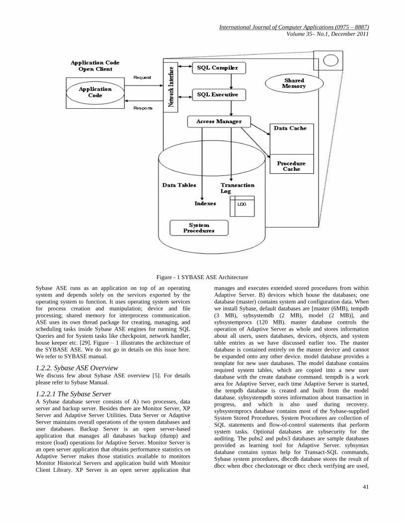
What remains after all other memory needs have been met is
available for the procedure cache and the data cache. Figure-2
shows how memory is divided [27].
Figure-2 How Adaptive Server uses memory
2.5. Server Performance Gains Through
Query Optimization [27,28] It is very important in this paper to discuss well about table,
index and page as these are very important for better Server
Performance Tuning and Query Optimization.
The Adaptive Server optimizer attempts to find the most
efficient access path to our data for each table in the query, by
estimating the cost of the physical I/O needed to access the data,
and the number of times each page needs to be read while in the
data cache.
In most database applications, there are many tables in the
database, and each table has one or more indexes. Depending on
whether we have created indexes, and what kind of indexes we
have created, the optimizer‘s access method options include:
A table scan – reading all the table‘s data pages, sometimes
hundreds or thousands of pages. Index access – using the index
to find only the data pages needed, sometimes as few as three or
four page reads in all. Index covering – using only a non
clustered index to return data, without reading the actual data
rows, requiring only a fraction of the page reads required for a
table scan.
Having the proper set of indexes on our tables should allow
most of our queries to access the data they need with a minimum
number of page reads.
2.5.1. Query Processing and Page Reads Most of a query‘s execution time is spent reading data pages
from disk. Therefore, most of our performance improvement —
more than 80%, according to many performance and tuning
experts — comes from reducing the number of disk reads
needed for each query.
2.5.2. Adaptive Server pages The basic unit of storage for Adaptive Server is a page. Page
sizes can be 2K, 4K, 8K to 16K. The server‘s page size is
established when we first build the source. Once the server is
built the value cannot be changed. These types of pages store
database objects:
Data pages – store the data rows for a table, Index pages – store
the index rows for all levels of an index and Large object (LOB)
pages – store the data for text and image columns, and for Java
off-row columns.
2.5.3. Extents Adaptive Server pages are always allocated to a table, index, or
LOB structure. A block of 8 pages is called an extent. The size
of an extent depends on the page size the server uses. The extent
size on a 2K server is 16K where on an 8K it is 64K, etc. The
smallest amount of space that a table or index can occupy is 1
extent, or 8 pages. Extents are deallocated only when all the
pages in an extent are empty.
The use of extents in Adaptive Server is transparent to the user
except when examining reports on space usage.
2.5.4. Allocation Pages When we create a database or add space to a database, the space
is divided into allocation units of 256 data pages. The first page
in each allocation unit is the allocation page. Page 0 and all
pages that are multiples of 256 are allocation pages.
The allocation page tracks space in each extent on the allocation
unit by recording the object ID and index ID for the object that
is stored on the extent, and the number of used and free pages.
The allocation page also stores the page ID for the table or
index‘s OAM page.

International Journal of Computer Applications (0975 – 8887)
Volume 35– No.1, December 2011
46
2.5.5. Object Allocation Map Pages Each table, index, and text chain has one or more Object
Allocation Map (OAM) pages stored on pages allocated to the
table or index. If a table has more than one OAM page, the
pages are linked in a chain. OAM pages store pointers to the
allocation units that contain pages for the object.
The first page in the chain stores allocation hints, indicating
which OAM page in the chain has information about allocation
units with free space. This provides a fast way to allocate
additional space for an object and to keep the new space close to
pages already used by the object.
2.5.6. How Indexes Work We discuss here Adaptive Server stores indexes and how it uses
indexes to speed data retrieval for select, update, delete, and
insert operations.
Indexes are the most important physical design element in
improving database performance and mainly are 1) Indexes help
prevent table scans. Instead of reading hundreds of data pages, a
few index pages and data pages can satisfy many queries, 2) For
some queries, data can be retrieved from a nonclustered index
without ever accessing the data rows, 3) Clustered indexes can
randomize data inserts, avoiding insert ―hot spots‖ on the last
page of a table and 4) Indexes can help avoid sorts, if the index
order matches the order of columns in an order by clause.
In addition to their performance benefits, indexes can enforce
the uniqueness of data.
Indexes are database objects that can be created for a table to
speed direct access to specific data rows. Indexes store the
values of the key(s) that were named when the index was
created, and logical pointers to the data pages or to other index
pages.
Although indexes speed data retrieval, they can slow down data
modifications, since most changes to the data also require
updating the indexes. Optimal indexing demands are 1) An
understanding of the behavior of queries that access unindexed
heap tables, tables with clustered indexes, and tables with
nonclustered indexes, 2) An understanding of the mix of queries
that run on our server and 3) An understanding of the Adaptive
Server optimizer.
2.5.7. How Indexes Affect Performance Carefully considered indexes, built on top of a good database
design, are the foundation of a high-performance Adaptive
Server installation. However, adding indexes without proper
analysis can reduce the overall performance of our system.
Insert, update, and delete operations can take longer when a
large number of indexes need to be updated.
Analyze our application workload and create indexes as
necessary to improve the performance of the most critical
processes.
The Adaptive Server query optimizer uses a probabilistic costing
model. It analyzes the costs of possible query plans and chooses
the plan that has the lowest estimated cost. Since much of the
cost of executing a query consists of disk I/O, creating the
correct indexes for our applications means that the optimizer can
use indexes to 1) Avoid table scans when accessing data, 2)
Target specific data pages that contain specific values in a point
query, 3) Establish upper and lower bounds for reading data in a
range query, 4) Avoid data page access completely, when an
index covers a query and 5) Use ordered data to avoid sorts or to
favor merge joins over nested-loop joins.
In addition, we can create indexes to enforce the uniqueness of
data and to randomize the storage location of inserts.
2.5.8. Types of Indexes Adaptive Server provides two types of indexes; 1) Clustered
indexes, where the table data is physically stored in the order of
the keys on the index such as for allpages-locked tables, rows
are stored in key order on pages, and pages are linked in key
order and for data-only-locked tables, indexes are used to direct
the storage of data on rows and pages, but strict key ordering is
not maintained and 2) Nonclustered indexes, where the storage
order of data in the table is not related to index keys.
We can create only one clustered index on a table because there
is only one possible physical ordering of the data rows. We can
create up to 249 nonclustered indexes per table.
A table that has no clustered index is called a heap. The rows in
the table are in no particular order, and all new rows are added
to the end of the table.
2.5.9. Index Pages Index entries are stored as rows on index pages in a format
similar to the format used for data rows on data pages. Index
entries store the key values and pointers to lower levels of the
index, to the data pages, or to individual data rows.
Adaptive Server uses B-tree indexing, so each node in the index
structure can have multiple children.
Index entries are usually much smaller than a data row in a data
page, and index pages are much more densely populated than
data pages. If a data row has 200 bytes (including row
overhead), there are 10 rows per page.
An index on a 15-byte field has about 100 rows per index page
(the pointers require 4–9 bytes per row, depending on the type of
index and the index level).
Indexes can have multiple levels 1) Root level, 2) Leaf level and
3) Intermediate level.
Root level: The root level is the highest level of the index. There
is only one root page. If an allpages-locked table is very small,
so that the entire index fits on a single page, there are no
intermediate or leaf levels, and the root page stores pointers to
the data pages. Data-only-locked tables always have a leaf level
between the root page and the data pages. For larger tables, the
root page stores pointers to the intermediate level index pages or
to leaf-level pages.
Leaf level: The lowest level of the index is the leaf level. At the
leaf level, the index contains a key value for each row in the
table, and the rows are stored in sorted order by the index key.
For clustered indexes on allpages-locked tables, the leaf level is
the data. No other level of the index contains one index row for
each data row. For nonclustered indexes and clustered indexes
on data-only-locked tables, the leaf level contains the index key
value for each row, a pointer to the page where the row is stored,
and a pointer to the rows on the data page. The leaf level is the

International Journal of Computer Applications (0975 – 8887)
Volume 35– No.1, December 2011
47
level just above the data; it contains one index row for each data
row. Index rows on the index page are stored in key value order.
Intermediate level: All levels between the root and leaf levels
are intermediate levels. An index on a large table or an index
using long keys may have many intermediate levels. A very
small allpages-locked table may not have an intermediate level
at all; the root pages point directly to the leaf level.
Please see manual in details about Clustered indexes and select
operations, Clustered indexes and insert operations, Clustered
indexes and delete operations, Nonclustered indexes and select
operations, Nonclustered indexes and insert operations,
Nonclustered indexes and delete operations.
2.5.10. New Optimization Techniques and Query
Execution Operator Supports in ASE The query optimizer provides speed and efficiency for online
transaction processing (OLTP) and operational decision-support
systems (DSS) environments. We can choose an optimization
strategy that best suits our query environment. Query optimizer
uses a number of algorithms and formulas. The information
needed by the optimizer is supplied by the statistics.
The query optimizer is self-tuning, and requires fewer
interventions than versions of Adaptive Server Enterprise earlier
than 15.0. It relies infrequently on worktables for materialization
between steps of operations; however, the query optimizer may
use more worktables when it determines that hash and merge
operations are more effective.
Some of the key features in the release 15.0 query optimizer
include support for 1) New optimization techniques and query
execution operator supports that enhance query performance,
such as a) On-the-fly grouping and ordering operator support
using in-memory sorting and hashing for queries with group by
and order by clauses b) hash and merge join operator support for
efficient join operations and c) index union and index
intersection strategies for queries with predicates on different
indexes, 2) Improved index selection, especially for joins with
or clauses, and joins with and search arguments (SARGs) with
mismatched but compatible datatypes, 3) Improved costing that
employs join histograms to prevent inaccuracies that might
otherwise arise due to data skews in joining columns, 4) New
cost-based pruning and timeout mechanisms in join ordering and
plan strategies for large, multiway joins, and for star and
snowflake schema joins, 5) New optimization techniques to
support data and index partitioning (building blocks for
parallelism) that are especially beneficial for very large data
sets, 6) Improved query optimization techniques for vertical and
horizontal parallelism and 7) Improved problem diagnosis and
resolution through a) Searchable XML format trace outputs, b)
Detailed diagnostic output from new set commands.
List of optimization techniques and operator support provided in
Adaptive Server Enterprise are hash join, hash union distinct,
merge join, merge union all, merge union distinct, nested-loop-
join, append union all, distinct hashing, distinct sorted, group-
sorted, distinct sorting, group hashing, multi table store ind,
opportunistic distinct view, index intersection. Please see
manuals for these techniques and operators in details. Please see
details work on join in [30].
3. QUERY PROCESSING AND
OPTIMIZATION OF QUERY
PROCESSING
3.1. Query Processing and Optimization In modern database systems queries are expressed in a
declarative query language such as SQL or OQL. The users need
only specify what data they want from the database, not how to
get the data. It is a task of database management system
(DBMS) to determine an efficient strategy for evaluating a
query. Such a strategy is called an execution plan. A substantial
part of the DBMS constitutes the query optimizer which is
responsible for determining an optimal execution plan. Query
optimization is a difficult task since there usually exist a large
number of possible execution plans with highly varying
evaluation costs [24].
We can say Query Plan is the set of instructions describing how
the query will be executed. This is the optimizer‘s final decision
on how to access the data. Costing is the process the optimizer
goes through to estimate the cost of each query plan it examines.
Optimizer uses two phases to find the cheapest query plan and
are 1) Index selection phase and 2) Search engine phase. Please
see details in [31].
The core of query optimization is algebraic query optimization.
Queries are first translated into expression over some algebra.
These algebraic expressions serve as starting point for algebraic
optimization. Algebraic optimization uses algebraic rewrite rules
(or algebraic equivalences) to improve a given expression with
respect to all equivalent expressions (expressions that can be
obtained by successive applications of rewrite rules). Algebraic
optimization can be heuristic or cost-based. In heuristic
optimization a rule improves the expression most of the time
(but not always). Cost-based optimization however uses a cost
function to guide the optimization process. ASE uses cost-based
optimization. Among all equivalent expression an expression
with minimum cost is computed. The cost function constitutes a
critical part of a query optimizer. It estimates the amount of
resources needed to evaluate a query. Typically resources are
CPU time, the number of I/O operations, or the number of pages
used for temporary storage (buffer/disk page).
Without optimization, some queries might have excessively high
processing cost.
We can also say query processing is a process of transforming a
high level and non procedure query/language such as SQL into a
plan (procedural specification) that executes and retrieve data
from the database. It involves four phases which are query
decomposition (scanning, parsing and validating), query
optimization, code generation and run time query execution
[22,25,26,36]. The scanner identifies the language token- such
as SQL keywords, attribute names and relation names – in the
text of the query, whereas parser checks the query syntax to
determine whether it is formulated according to the syntax rules
(rules of grammar) of the query language. The query must also
be validated, by checking that all attributes and relation names
are valid and semantically meaningful names in the schema of
the particular database being queried. We do not discuss in
details here in this paper. Figure 3 shows the query processing
strategy.

International Journal of Computer Applications (0975 – 8887)
Volume 35– No.1, December 2011
48
We can also say query optimization is the process of choosing
the efficient execution strategy for execution a query. In
systematic query optimization, the system estimates the cost of
every plan and then chooses the best one. The best cost plan is
not always universal since it depends on the constraints put on
data. The cost considered in systematic query optimization
includes access cost to secondary storage, storage cost,
computation cost for intermediate relations and communication
cost.
In ASE 15 the query processing engine has been enhanced to
include very efficient techniques. ASE 15 incorporates into
optimizer component of the query processing engine proven and
well tested ‗start-of-the-art‘ technology. ASE 15 performs very
well out of the box by automatically analyzing and selecting
high performance query plan using much wider array of options
and methods than were available in earlier versions [20].
Optimization Goals are provided in ASE 15 in order to allow
query optimization behavior to fit the needs of our application.
The optimization goals are groupings of pre-set optimization
criteria that in combination affect the overall behavior of the
optimizer component of the query processing engine. Each of
the goals is designed to direct the optimizer to use features and
functionality that will allow it to find the most efficient query
plan.
There are three optimization goals that can be set. The first is
designed to allow the query processing engine to use all the
techniques available, including the new features and
functionality to find and execute the most efficient query plans.
This goal optimizes the complete result set and balances the
needs of both OLTP and DSS style queries; it is on by default.
The second optimizer goal will allow the query processing
engine to use those techniques most suitable to finding the most
efficient query plan for purely OLTP query.
The third optimization goal is designed to generate query plans
that will return the first few rows of the result set as quickly as
possible. This goal is very efficient in cursor-based and web-
based applications.
These optimization goals are designed to be set at the server-
wide level. However, they can also set at the session or query
level for testing purposes. Once set there should be no further
need to tune the query processing engine‘s behavior for the
environment we have chosen.
To start with query processing and optimization, first we
execute:
set showplan on
go
set statistics io on
go
then we run our query. We check if the query plan chooses the
indexes we expected. We check the logical I/Os for each table
and look for unexpected (i.e. high) values.
Steps to tune our query involved our database is normalized, our
SQL code is reasonably well designed, the ASE resources have
been allocated appropriately for (a) the system and (b) our
database, the indices on the table(s) in the query are correct and
the table(s) in each query are implemented correctly (physical
attributes).
SET FORCEPLAN ON instructs the Optimizer to use the order
we have listed in the FROM clause.
SET STATISTICS IO ON, SET STATISTICS TIME ON is
important when tuning.

International Journal of Computer Applications (0975 – 8887)
Volume 35– No.1, December 2011
49
Figure 3 Query Processing and Optimization
3.2. Abstract Query Plans (APs) ASE introduces a new and powerful feature, Abstract Query
Plans (APs) [11]. This is a very large feature which cannot be
fully covered here. Please also see [12,13,23]. APs are persistent
human-readable and editable copy of the query plan created by
the optimizer. APs can be captured when a query is run. Once
captured, they can then be associated to their originating query
and used to execute that query whenever it is run again. This
features allow us to run a query, capture and save the query plan
created by the query optimizer and then reuse it whenever the
same query is run again. We can edit an Abstract Plan, thus
telling the optimizer exactly what to do, or simply use it as is.
This is a very powerful and flexible feature.
We can say abstract plan is a description of a query plan which
is kept in persistent storage, can be read and edited, and is
associated with a specific query. When executing that query, the
optimizer‘s plan will be based on the information in the abstract
plan. We cannot generate abstract plans on pre ASE 12.0 server.
We turn on the AP capture mode and run the slow-performing
query(s) to capture APs. Then we examine the AP to identify
any possible problem. We edit the plan, creating a partial or full
AP to resolve the issue. We make sure the AP is used whenever
we run the query.
Before we go into APs in detail, let‘s back up a bit and define
query plans and their role in executing a query. The optimizer‘s
job is to determine the most efficient way (method) to access the
data and pass this information on for execution of the query. The
query plan is the information on how to execute the query,
which is produced by the optimizer. Basically, the query plan
contains a series of specific instructions on how to most
efficiently retrieve the required data. Prior to ASE 12.0, the only
option has been to view it via showplan or dbcc traceon 310
output (as FINAL PLAN). In most cases, changes to the
optimizer‘s cost model result in more efficient query plans. In
some cases, of course, there will be no change; and in some
there may be performance regression. APs can be captured
before applying the upgrade, and then, once the upgrade has
been completed, queries can be rerun to see if there is any
negative change in performance. If a performance regression is
identified after the upgrade, the AP from previous version can
then be used in the newer version to run the query and we can
contact Sybase regarding the problem. In the case of possible
optimization bug, we may write an AP to workaround the
problem while Sybase investigates it.
Once execution is complete, the query plan is gone. In ASE
12.0, however, APs make each query plan fully available to us.
They can be captured, associated to their original query, and
reused over and over, bypassing the optimizer fully or partially.
They can even be edited and included in a query using the new
T-SQL PLAN statement as we have stated earlier. Abstract
Query Plan was first introduced in ASE 12.0 version.
When ASE creates an AP, it contains all the access methods
specified by the optimizer such as how to read the table (table or
index scan), which index to use if an index scan is specified,
which join type to use if a join is performed, what degree of
parallelism, what I/O size, and whether the LRU or MRU
strategy is to be utilized.
Let‘s take a quick look at a couple of simple APs.
select * from t1 where c=0

International Journal of Computer Applications (0975 – 8887)
Volume 35– No.1, December 2011
50
The simple search argument query above generates the AP
below:
(i_scan c_index t1)
( prop t1 ( parallel 1 )( prefetch 16 )( lru ))
This AP says access table t1 is using index c_index. It also says
that table t1 will be accessed using no parallelism, 16K I/O
prefetch, and the LRU strategy.
select * from t1, t2
where t1.c = t2.c and t1.c = 0
The simple join above results in the AP below:
(nl_g_join t1.c = t2.c and t1.c = 0 (i_scan i1 t1) (i_scan i2 t2)
( prop t1 ( parallel 1 )( prefetch 2 )( lru )
( prop t2 ( parallel 1 )( prefetch 16 )( lru ))
This AP says to perform a nested loop join, using table t1 as the
outer table, and to access it using an index i1. Use table t2 as the
inner table; access it using index i2. For both tables, use no
parallelism and use the LRU strategy. For table t1, use 2K
prefetch and for table t2, use 16K prefetch. As we can see, with
a little practice APs are easy to read and understand.
APs are captured when we turn on the capture mode.
set plan dump on
ASE configuration value:
sp_configure "abstract plan dump", 1
The optimizer will optimize the query as usual, but it will also
save a copy of its chosen query plan in the form of an AP. Keep
in mind that if we are capturing an AP for a compiled object,
such as stored procedure, we will need to ensure that it is
recompiled. We can do this by executing it with recompile or by
dropping and recreating it and then executing again.
As APs are captured, they are written to the new system table
sysqueryplans and placed in a capture group.
When an AP is captured, it is stored along with a unique AP ID
number, a hash key value, the query text (trimmed to remove
white space), the user‘s ID, and the ID of the current AP group.
The hash key is a computed number used later to aid when
associating the query to an AP, created using the trimmed query
text. In general, there are atleast one million possible hash key
values for every AP, thus making conflicts unlikely.
APs can also be created manually without conflict by using the
new create plan T-SQL statement, writing the AP text along
with the SQL statement. When we save an AP using the create
plan command, the query will not be executed. It‘s advisable to
run the query as soon as possible using the AP to ensure that it
performs the way we expect it to. Let‘s take a look:
create plan
select c1, c2 from tableA
where c1 = 10
and c2 > 100
"(i_scan tableA_index tableA)"
The AP in this example will access tableA using index
tableA_index.
There are many more related to APs, please see the Sybase
manual.
3.3. Optimization of Query Processing Query optimization is the process of analyzing a query to
determine what resources it requires and how the execute the
query with the least possible query cost. To understand the
optimization a query, we need to understand how the query
accesses database objects, the sizes of the objects, and the
indexes on the tables in order to determine whether it is possible
to improve the query‘s performance [2]. Please also see [12].
Symptoms of optimization problems are a query runs more
slowly than we expect, based on indexes and table size, a query
runs more slowly than similar query, a query suddenly starts
running more slowly than usual, a query processed within a
stored procedure takes longer than when it is processed as an
adhoc statement and the query plan shows the use of a table scan
when we expect it to use an index.
Source of optimization problems are statistics have not been
updated recently so the actual data distribution does not match
the values used by Adaptive Server to optimize queries, the rows
to be referenced by a given transaction do not fit the pattern
reflected by the index statistics, an index is being used to access
a large portion of the table, where clauses are written in
unoptimizable form, no appropriate index exists for a critical
query and a stored procedure was compiled before significant
changes to the underlying tables were performed.
ASE 15 introduces completely new Optimizer and Query
Processing engines, incorporating many fundamental changes.
With these improvements comes the requirement that we give
the optimizer as much accurate information about our data and
databases as we possibly can. All that the optimizer needs to
know is found in the ‗statistics‘. ASE 15‘s optimizer
incorporates state of the art technology. A great deal of highly
skilled and dedicated work went into the huge project of
redesigning and rewriting it. It will produce amazing
performance levels as long as it gets the most accurate
information about our data as possible. The statistics contain
everything the optimizer needs to do its job quickly and
efficiently [7].
Before we continue let‘s quickly review exactly what statistics
are available to the optimizer. There are two types of statistics –
column level and object level. The column level statistics
describe the distribution of values in the column; they consist of
the column‘s histogram and density values and are updated
when an index is created or an ‗update statistics‘ command is
run. The object level statistics describe a table and its indexes
and include values such as number of rows and pages in the
table and/or index (es), the number of empty pages, and the
cluster ratios among others. Some of the object level statistics
are updated automatically by ASE, others when ‗update
statistics‘ is run.
3.3.1. Factors analyzed in optimizing queries Query plans consist of retrieval tactics and an ordered set of
execution steps, which retrieve the data needed by the query. In
developing query plans, the query optimizer examines:
1) The size of each table in the query, both in rows and data
pages, and the number of OAM and allocation pages to be read,
2) The indexes that exist on the tables and columns used in the

International Journal of Computer Applications (0975 – 8887)
Volume 35– No.1, December 2011
51
query, the type of index, and the height, number of leaf pages,
and cluster ratios for each index, 3) The index coverage of the
query; that is, whether the query can be satisfied by retrieving
data from the index leaf pages without accessing the data pages.
Adaptive Server can use indexes that cover queries, even if no
where clauses are included in the query, 4) The density and
distribution of keys in the indexes, 5) The size of the available
data cache or caches, the size of I/O supported by the caches,
and the cache strategy to be used, 6) The cost of physical and
logical reads; that is, reads of physical I/O pages from the disk,
and of logical I/O reads from main memory, 7) join clauses,
with the best join order and join type, considering the costs and
number of scans required for each join and the usefulness of
indexes in limiting the I/O, 8) Whether building a worktable (an
internal, temporary table) with an index on the join columns is
faster than repeated table scans if there are no useful indexes for
the inner table in a join, 9) Whether the query contains a max or
min aggregate that can use an index to find the value without
scanning the table and, 10) Whether data or index pages must be
used repeatedly, to satisfy a query such as a join, or whether a
fetch-and-discard strategy should be employed to avoid flushing
of the buffer cache of useful pages of other tables, since the
pages of this table need to be scanned only once.
For each plan, the query optimizer determines the total cost by
computing the costs of logical and physical I/Os, and CPU
processing. If there are proxy tables, additional network related
costs are evaluated as well. The query optimizer then selects the
cheapest plan.
Statements in a stored procedure or trigger are optimized when
the respective statements are first executed, and the query plan is
stored in the procedure cache. If a respective statement is not
executed, then it will not be optimized until a later execution of
the stored procedure in which the statement is executed. If other
users execute the same procedure while an unused instance of a
stored procedure resides in the cache, then that instance is used,
and previous executed statements in that stored procedure are
not recompiled [35].
3.3.2. Why Creating and Maintaining Accurate
Statistics is Important to ASE 15 The optimizer has always been dependant on the statistics
because it is ‗cost based‘. That is, it makes its decisions about
which query plan to use based on the estimated resource costs of
executing it. Without them it‘s flying blind and can only guess at
which is the most efficient query plan.
In fact, the statistics have become even more critical to good
performance. Why is this? Because many of the optimizer‘s new
features and functionality can be very I/O intensive, especially if
an inefficient query plan is used. Some of the new features and
functionality include new methods for handling groupings,
unions and all query level sorting operations.
New and improved join processing that is sensitive to the
accuracy of the statistics has also been added. Hash joins are
new to ASE and Sort-Merge joins have been improved and are
turned on by default in ASE 15 [28]. If there are no useful
indexes or if the statistics tell the optimizer that an index would
not be efficient to use, then a worktable has to be created for the
join. Joining values are moved into the worktable where they are
sorted into the order required by the join and then merged with
rows from the other joining table. All this, especially the sorting
of the values in the worktable requires a great deal of I/O. Since
both of these join methods can include sorting steps it is
imperative that efficient query plans are chosen by the
optimizer. The bottom-line is that large, unnecessary sorts are
the bane of good query performance. It can‘t be over
emphasized how important it is to keep accurate statistics
available for the optimizer to take advantage of when estimating
the costs of joins. Even though ASE 15 is designed to avoid
worktables that were often used in earlier versions, inaccurate
statistics can lead to query plans that revert to using them.
One new piece of functionality added to ASE 15 in order to deal
directly with a long-standing join performance issue is Join
Histograms.
3.3.3. Join Histograms The Problem - Prior to ASE 15 the optimizer could only use a
column‘s density value, if it was available, to estimate the cost
of joining one column to another. The density value is a
‗weighted average‘ of the distribution of values in the column. If
there was no density value, the optimizer used a preset
selectivity value, a sort of ‗magic number‘ that was based on the
join operator. Since the most common join is an equi-join, the
‗magic number‘ used was 0.10 (the optimizer believed that 10%
of the rows in the column qualified for the join). As we might
imagine most joins don‘t qualify exactly 10% of either column.
When the column contained a fairly even distribution of values,
the density value was accurate. However, when the column
contained any degree of data skew (many values occupying a
small number of rows each and a few values occupying many
rows each) the density value was not accurate. When the
optimizer used a density value of a skewed column it would lead
the optimizer to believe that a join of the skewed table would be
more efficient than it actually was. This in turn resulted in some
very poorly performing joins.
The ASE 15 Solution - The join histograms of ASE 15 always
give the optimizer an accurate view of the table. For example if
the where clause of a join statement disqualifies a highly
duplicated value it is not included in the join histogram; why
estimate the cost of retrieving the skewed values if they aren‘t
needed for the join? How do join histograms work? Very simply
– If there are statistics on a column that is being joined and there
is a search argument (SARG) in the query then a histogram will
be built on the fly containing only the values that the SARG has
qualified.
A quick example: customerID table contains 100 distinct
customer ids, orderID table contains all the orders placed by the
100 customers, 100K rows. Let‘s say that of the 100 customers 3
have placed 50% of all the orders and of the 3 all have placed
close to the same number of orders; the orderID table will
contain data skew while the customerID table will be evenly
distributed.
In pre-ASE 15, the density value would be larger due to the
highly duplicated values for the three big customers. There is a
good chance that the optimizer would estimate that an index on
the custID column in the orders table would be expensive to use
and call for a table scan. In fact, the index would be very
selective for the query. In ASE 15, the join histogram would not
include the highly duplicated values thus accurately making the
index access look cheaper than a table scan.

International Journal of Computer Applications (0975 – 8887)
Volume 35– No.1, December 2011
52
Of course, for join histograms to be accurate and useful,
accurate statistics need to be in place for the joining columns.
Here‘s another situation that missing or inaccurate statistics can
cause – The optimizer having to examine more query plans than
is necessary [13].
3.3.4. Timeout The Problem – In ASE 15 the new functionality in the optimizer
can lead to the optimizer having MANY more query plans to
examine than in earlier versions. Add to this the large and
complex queries common today and the optimizer is working
much harder than ever before. The more query plans to estimate
costs for, the more time it takes to find the best plan to execute.
In fact, there is a possibility that the optimizer can take more
time optimizing the query than it takes to actually execute it and
return the results.
The ASE 15 Solution - It is for this reason that ‗timeout‘ was
included in the ASE 15 optimizer. Put simply, once the
optimizer has reached the timeout limit it will choose the
cheapest (most efficient) query plan it has examined up to that
point. This plan will be used to execute the query whether it‘s
the best or not. Accurate statistics can result in the optimizer
having to examine far fewer query plans and finding the most
efficient plan before the timeout limit is reached. This in turn
will result in less procedure cache usage for the optimizer‘s
search. When there are no statistics or the statistics are
inaccurate the optimizer can overestimate the cost of what is
actually the best query plan and go on to examine many more
[13].
3.3.5. How to Create and Maintain Accurate
Statistics Statistics are kept up to date by regularly running the update
statistics command, or by dropping and recreating indexes,
which can be very time and resource consuming. In the past,
there were a number of ‗rules of thumb‘ floating around among
DBAs about when to update statistics. Some of the more popular
were 1) when 5-10% of the data has changed, 2) once a week, 3)
every day, 4) only when queries start performing badly, 4) only
when we have time to do it and 5) We never run update
statistics, etc.
The honest answer to the question was, is, and will always be -
It all depends on our data and our queries [13].
3.4.6. Locking and Concurrency The Optimizer decides on Lock Type and Granularity. Decisions
on lock type (share, exclusive, or update) and granularity (page
or table) are made during optimization so make sure our updates
and deletes don't scan the table. Exclusive Locks are only
released upon Commit or Rollback. Lock Contention can have a
large impact on both throughput and response time if not
considered both in the application and database design. Keep
transactions as small and short as possible to minimize blocking.
Consider alternatives to "mass" updates and deletes such as a
v10.0 cursor in a stored procedure which frequently commits.
Never include any "user interaction" in the middle of
transactions. Shared Locks generally released after page is read.
Share locks "roll" through result set for concurrency. Only
"HOLDLOCK" or "Isolation Level 3" retains share locks until
commit or rollback. Remember also that HOLDLOCK is for
read-consistency. It doesn't block other readers. Use optimistic
locking techniques such as timestamps and the tsequal() function
to check for updates to a row since it was read (rather than
holdlock)[8].
3.4.7. Tuning Transact-SQL Queries Poor Performance SQL problem can occur at any stage of the
development lifecycle, but catching them early is always much
less expensive that letting them reach a production environment.
Often times, the main bottleneck is a SQL statement taking up
too many resources then we examine the following 1) Are the
table and index statistics up to date? 2) Are there any missing
indexes? 3) Do any of the columns need extended histogram or
frequency statistics? 4) Are all the unique and not-null
constraints correctly defined on the columns and tables? 5) Is the
database choosing the right access path? [21].
One of the largest factors determining performance is TSQL.
Test not only for efficient plans but also semantic correctness.
3.4.8. Normalized -vs- Denormalized Always start with a completely normalized database.
Denormalization should be an optimization taken as a result of a
performance problem. Benefits of a normalized database
include; reduce data redundancy, accelerates searching, sorting,
and index creation since tables are narrower, allows more
clustered indexes and hence more flexibility in tuning queries,
since there are more tables, accelerates index searching since
indexes tend to be narrower and perhaps shorter, allows better
use of segments to control physical placement of tables, fewer
indexes per table, helping UPDATE, INSERT, and DELETE
performance, fewer NULLs and less redundant data, increasing
compactness of the database, accelerates trigger execution by
minimizing the extra integrity work of maintaining redundant
data, joins are generally very fast provided proper indexes are
available, cost of a logical I/O (get page from cache) only 1-2
milliseconds. We can say benefits of normalization mainly are
1) More rows per page (less logical I/O), 2) More rows per I/O
(more efficient), and 3) More rows fit in cache (less physical I/).
There are some good reasons to denormalize; all queries require
access to the "full" set of joined data, majority of applications
scan entire tables doing joins, computational complexity of
derived columns require storage for SELECTs [8]. We have also
discussed well in section 4.13. For details please see [15].
3.4.9. Index Selection Without a clustered index, all INSERTs and "out-of-place"
UPDATEs go to the last page. The lock contention in high
transaction environments would be prohibitive. This is also true
for INSERTs to a clustered index on a monotonically increasing
key.
High INSERT environments should always cluster on a key
which provides the most "randomness" (to minimize lock /
device contention) that is usable in many queries. Note this is
generally not our primary key!
Prime candidates for clustered index (in addition to the above)
include: Columns Accessed by a Range, Columns Used with
Order By, Group By, or Joins
Indexes Help SELECTs and Hurt INSERTs
Too many indexes can significantly hurt performance of
INSERTs and "out-of-place" UPDATEs.
International Journal of Computer Applications (0975 – 8887)
Volume 35– No.1, December 2011
53
Prime candidates for non-clustered indexes include; Columns
Used in Queries requiring Index Coverage, Columns Used to
Access Less than 20% (rule of thumb) of the Data, Unique
indexes should be defined as UNIQUE to help the optimizer,
minimize index page splits with fill factor (helps concurrency
and minimizes deadlocks), Keep the Size of the Key as Small as
Possible, Accelerates index scans and tree traversals
Use small datatypes whenever possible. Numerics should also
be used whenever possible as they compare faster than strings.
For details please see [27].
4. ILLUSTRATING SOLUTIONS TO
SOME SITUATIONS NORMALLY
OCCURS DURING SERVER RUN TIME
RELATED TO THE SERVER
PERFORMANCE TUNING AND QUERY
OPTIMIZATION This section is illustrating solutions to some situations normally
occurs during server run time to obtain better server
performance and query optimization. Following two system
procedures that we always use during server monitoring and
performance tuning:
sp_sysmon a system procedure that monitors Adaptive Server
performance and provides statistical output describing the
behavior of our Adaptive Server system. Mainly we use
sp_sysmon to look buffer hit ratio and spinlock contention.
Buffer hit ratio reports the % times a requested datapage is
found in the data caches. A buffer hit ratio of less than 97%
could indicate memory starvation. If sufficient amount of
memory is not allocated to the data cache the first thing to do
would be to increase memory. Spinlock Contention reports the
number of times an engine encountered spinlock contention on
the cache, and had to wait to acquire memory. Splitting the data
caches into cachelets will reduce spinlock contention in case of
SMP environments.
sp_monitor a system procedure displays statistics about
Adaptive Server. It is a well known stored procedure available
for the longest time on ASE to capture CPU busy and IO busy
statistics since the last run of the same procedure. This for me
provides a first insight at what is going on in the data server as
far as IO and CPU utilization is concerned. Besides this stored
procedure, there are some other features that can help us for
performance troubleshooting.
We have discussed about sp_sysmon and sp_monitor in section
2.1.7 also. For details please refer to Sybase manual.
4.1. We normally use following tools to
evaluate and tune query We use the "set showplan on" command to see the plan chosen
as "most efficient" by optimizer. We run all queries through
during development and testing to ensure accurate access model
and known performance. Information comes through the Error
Handler of a DB-Library application. We can also say set
showplan on is used for look for table scans in the results. We
can also say showplan enables us to find out which plan the
optimizer has chosen, what indexes it intends to use, and which
tables will be accessed most heavily. Given this knowledge, we
could alter our queries, create indexes, or alter our table design,
caching etc to improve application performance. We use set
noexec on, so that the showplan is returned, but the server does
not actually return the data. We show here an example.
select * into #dennis from sysobjects
go
set showplan on
set noexec on
go
select name from #dennis where type = ‗U‘ order by name
go
We use the "dbcc traceon(3604, 302, 310)" command to see
each alternative plan evaluated by the optimizer. Generally, this
is only necessary to understand why the optimizer won't give us
the plan we want. If we think the problem is with an index, here
is how to see they are chosen using dbcc traceon(302) and dbcc
traceon(310).
We use the "set statistics io on" command to see the number of
logical and physical i/o's for a query. Scrutinize those queries
with high logical i/o's and it usually takes a lot of time.
We use the "set statistics time on" command to see the amount
of time (elapsed, execution, parse and compile) a query takes to
run or we can say it gathers time statistics so we can see where
the time is spent.
We use "set forceplan on" command to change join order to be
the order of the tables in the FROM clause.
If the optimizer refuses to select the proper index for a table, we
force it by adding the index id in parentheses after the table
name in the FROM clause.
SELECT * FROM orders(2), order_detail(1) WHERE ... [8]
We use set statistics subquerycache on to display the number of
cache hits and misses and the number of rows in the cache for
each subquery.
We also use optdiag utility command to display statistics for
tables, indexes, and columns. This utility allows us to read, write
and simulate the statistics used by the optimizer to determine the
most efficient method to retrieve the required data. Please see
details in [11,13].
We also use set table count that increases the number of tables
that the optimizer considers at one time while determining join
order.
Adaptive Server's cost-based optimizer uses statistics about the
tables, indexes, and columns named in a query to estimate query
costs. It chooses the access method that the optimizer determines
has the least cost. But this cost estimate cannot be accurate if
statistics are not accurate. For details please also see [12]. We
have also discussed well in section 3.3.1 and 3.3.2.
Some statistics, such as the number of pages or rows in a table,
are updated during query processing. Other statistics, such as the
histograms on columns, are only updated when we run the
update statistics command or when indexes are created.
We can use the optdiag command to see the time update
statistics was last run.
The update statistics commands update the column-related
statistics such as histograms and densities. So statistics need to

International Journal of Computer Applications (0975 – 8887)
Volume 35– No.1, December 2011
54
be updated on those columns where the distribution of keys in
the index changes in ways that affect the use of indexes for our
queries.
Running the update statistics commands requires system
resources. Like other maintenance tasks, it should be scheduled
at times when load on the server is light. In particular, update
statistics requires table scans or leaf-level scans of indexes, may
increase I/O contention, may use the CPU to perform sorts, and
uses the data and procedure caches. Use of these resources can
adversely affect queries running on the server if we run update
statistics at times when usage is high. In addition, some update
statistics commands require shared locks, which can block
updates.
4.2. To start with query processing and
optimization we first execute set showplan on
go
set statistics io on
go
then we run our query. We check if the query plan chooses the
indexes we expected. We check the logical I/Os for each table
and look for unexpected (i.e. high) values.
4.3. Checking how much time query taking The goal is to optimize a set of queries to run faster, improve
performance. By knowing the meaning of data we can help
query optimizer to develop a better query plan and in some cases
we can override the query optimizer to follow a certain query
plan.
Suppose we have a batch of queries, which we want to optimize.
First we need to identify which query is creating the problem
and then to identify where the problem lies in that query. Query
that is taking maximum time is the first we want to consider for
the optimization. To check which query is taking maximum time
to execute we place getdate() both before and after the query.
We identity the type of the query whether it is a data look-up
query or data modification query.
We use ‗set showplan on‘ to see what query plan is executed by
the SQL Server? If query is taking a lot of time to execute it is
not possible to execute it again and again. We use ‗set noexec
on‘ to just build the query plan and not to execute it. When these
two options are set SQL Server will parse the query, optimize it
and develop a query plan, but will not submit it to execute.
As SQL server uses cost based query optimizer, it‘s always
better to turn on the following options to check the statistics of
the query:
set statistics io on gives actual logical and physical page reads
incurred by the query.
set statistics time on gives total CPU and elapsed time to execute
a query and the time to parse and compile the query [40].
4.4. Server was running fine when starts and
if we find slow we can think of just few If query plans are used by query optimizers to execute a
Query/Stored Procedure. Over time the query plans become
outdated and are no longer efficient then we should run update
statistics <table name> and sp_recompile <table name>.
If the query optimizer does a table scans when it cannot resolve
a badly written query or Stored Procedure. Here query
optimization is the only solution for this. We try to find out such
queries by running them during off-peak time.
4.5. Increase RAM size and number of
concurrent user connections Every user will consume resources on the Sybase Server, which
reduces the amount of memory that Sybase has for itself. For
this we should increase RAM on our server and increase the
amount of memory dedicated to Sybase server. Increase the no.
of concurrent user connections.
4.6. Rebuild Reorg command improve
Performance We always clean-up tables that have been updated frequently by
using command rebuild reorg.
4.7. Checking whether query is using an
index We look at the query plan that is generated by the optimizer. We
check whether the optimizer is picking up proper indexes for the
SARG, OR clauses and Join operations. We see whether it is
using indexes to execute the query or not, and if yes which
indexes are used. If there is an index on the table and optimizer
is not using that index to resolve the query, we try to figure out
why optimizer is not using the index [40]. We have figured out
this issue in section 4.1, 4.2 and 4.8.
4.8. Checking whether statistics is up-to-date As a general advice, once the table gets 20% updated, we have
to run the update statistics for the table. Update statistics for a
table updates the distribution page [server keeps distribution
information for each index on a separate page in the datebase]
(so distribution statistics) for the indexes used in the table. We
use ‗update statistics‘ command to update the statistics for all
indexes on a table, using following commands:
To update the statistics of all the indexes related to the table:
update statistics Sales.SalesOrderDetail where Sales is a
database and SalesOrderDetailes is a table.
To update the statistics of a particular index on the table:
update statistics Sales.SalesOrderDetail
AK_SalesOrderDetail_rowguid where
AK_SalesOrderDetail_rowguid is an index under table
SalesOrderDetail
We run dbcc traceon 302 for getting the meta-information to
know how the query optimizer is handling the index selection
and OR clauses. We run dbcc traceon 310 for getting the meta-
information to know how query optimizer is picking up the join
order [40].
Again we run that query and see if it using the indexes or not. If
the query is still not using any indexes, and we think that an
index can be used to execute the query faster, we can force the
optimizer to use the index by specifying the index ID number
after the table name in the query. SQL Server would use that
index to satisfy the query. We can always use ‗set statistics io‘
option to verify whether there was an I/O savings over the
optimizers choice or not.

International Journal of Computer Applications (0975 – 8887)
Volume 35– No.1, December 2011
55
We identify which indexes to use to resolve the query: clustered
or non-clustered. Clustered index is better for range queries, if
data is in sorted order, column has number of duplicate values,
and column is frequently referenced in the order by clause. Non-
clustered index is better for single row lookups, queries
containing joins, queries with small range retrieval.
We keep following things in mind for the indexes 1) unless the
OR strategy is applied, SQL server uses only one index per table
to satisfy the query, 2) sometimes a table scan may be cheaper
than a candidate index in terms of total I/O. e.g. large range
retrievals on a non-clustered-index column and 3) a non-
clustered index that covers a query will be faster than a similarly
defined clustered index.
4.9. If we are using Join and Subquery If the query contains any joins, we look what is the join order
selected by the optimizer. Joins are performed as a set of nested
loops. Generally Join queries consume more memory than
subquery. Subquery involves the table creation so affects
performance, because of I/O fetches need for processing.
Subquery is always better than join if we have hardware
bottleneck (memory constraints). We check if we can replace
join with the subquery. But if we can scale up our hardware
(nowadays it is not a big deal) then we go with join.
Order in which the join is performed has effect on the total
number of I/O performed. By knowing the meaning of data we
can select a particular join order and we check if it improves
performance. We can force join order with the ‗set forceplan‘
option:
set forceplan {on / off}
It might be possible that optimizer was using different indexes
before forcing the join order, as certain indexes may not be
useful for certain join orders. As the number of table increases,
query optimizer takes more time to determine the join order. If
the optimizer is picking the proper join order but taking a lot of
time in determining the join order, we can force that particular
join order and save time. One another reason query not picking
up proper indexes may be ―set table count value‖ is set to lower
number but the number of tables involved in the join operations
is relatively higher [40]. We have also discussed in section 4.15.
4.10. We can avoid transaction logging under
some circumstances Another factor while optimizing the query is to avoid the
transaction log in data modification queries. In the following
cases we can avoid the transaction to be logged; 1) we use fast
BCP instead of slow BCP to avoid the data to be logged, 2) we
use truncate table instead of delete and 3) we use select into
instead of creating temporary table to avoid the transaction log
[40].
4.11. We should prefer dropping and
rebuilding index under some circumstances A table having indexes and triggers takes long time to perform
data modification queries. Depending on how important the
query is, we can think of dropping the indexes during the
daytime and rebuilding the indexes at end of the day. For these
types of queries, in many cases index usage is discouraged,
because the update statements.
If we need to perform large data modification its better to drop
indexes and rebuild indexes after the data modification operation
is performed.
Another factor we want to consider is whether query is using
any worktable/temporary table to resolve the query. Creating the
worktable to solve the query always take much time to process.
Queries containing ‗order by‘, ‗group by‘, ‗distinct‘ always uses
a worktable. We check if we can satisfy the query by avoiding
these clauses. Probable solutions to avoid these clauses are 1) if
column has a unique/primary key, then there is no need to
specify the ‗distinct‘ clause, 2) if we have more than four tables
to joins, it will definitely use a worktable to resolve the query.
We try to keep the number of tables to join to minimum. We try
to create subquery to avoid join of more than four tables, 3) if
there is an index on a column, which keeps the column sorted,
we don‘t need to specify ‗order by‘ clause in the query, 4) if we
know that data is unique, then there is no need to specify the
‗group by‘ clause in the query.
We check for the following scenarios in the where clause of the
query 1) negative Logic (!=, <>): negative logic always results
in the table scan unless index covering is applied, 2) calculated
comparison: if right side of an expression needs to be calculated
first, it will not be evaluated until it reaches the execution stage
and 3) if a query is frequently using computed expressions,
insert a column of the computed expression in the table. We
need to write a trigger to maintain that column. e.g. suppose a
query always calculates discounted price from a table, its better
to insert a column of discounted price in the table [40].
4.12. We should avoid trigger and adopt
stored procedure under some circumstances A trigger gets fired for every transaction. It is another overhead
in the query. Depending on how important the query is we can
drop triggers and write a store procedure for that. And at end of
the day we can run that stored procedure to perform the
operations performed by the trigger. e.g. During the day we need
to handle a lot of queries for OLTP, at that time we can consider
to drop the trigger and run stored procedure at end of the day
[40].
4.13. We should denormalize tables under
some circumstances Depending upon the type of queries we can think of de-
normalizing the tables. Denormalizing can improve performance
by 1) Minimizing the need of join, 2) Reducing the No. of
foreign keys on tables, 3) Reducing the No. of indexes, saving
storage space, and reducing data modification time, 4) Pre
computing aggregate values, that is computing them at data
modification time rather than at select time and 5) Reducing the
No. of tables (in some cases). Following are the options to de-
normalize the data depending upon the importance of the queries
1) Inserting calculated columns: it incurs another overhead to
maintain the calculated column value. When a data row is
inserted, we need to calculate the value of that column.
Depending upon the importance of the query we can insert a
calculated column, 2) Vertical merge of tables: If a query always
performs the join of two or more tables. It is better to merge the
tables and build a new table to satisfy that query faster. Again it
depends on how much important the query is and how we are
going to manage the duplicate data. Duplicating the data

International Journal of Computer Applications (0975 – 8887)
Volume 35– No.1, December 2011
56
improves the query to run faster but it incurs another overhead
to maintain the duplicate data, 3) Vertical split of tables: If query
always select certain columns from the table, its better to
separate the columns from the table and perform the query to
improve the performance, 4) Horizontal merge of tables: Merge
the data horizontally. e.g. If a query shows the transaction done
by the customer in the current month only and if the user wants
to see the record for certain months, we can horizontally
combine data from old transactions table and recent transactions
table to give the result and 5) Horizontal split of tables: Split the
data horizontally. e.g. in a online banking scenario, split the data
in most recent transactions and old transactions. We can just
show the most recent transactions, instead of showing the whole
transactions [40].
4.14. Query plan optimization ASE 15 Set Plan Commands allow us to set an optimization goal
which fits our database environment.
In Decision Support System and Reporting Environments if we
give the optimizer more time to compile a query plan through
set plan command is beneficial for optimization.
set plan opttimeoutlimit 999
where current optimization timeout limit for query optimization
is 999.
The range of values for opttimeoutlimit has been changed to 0 –
4000, with 0 indicating no optimization limit.
There are three new optimization goals in Sybase ASE and
Optimization goal can be chosen at the Server, Session and
Query level.
allrows_mix – the default goal, as well as the most useful goal in
a mixed query environment. It balances the needs of OLTP and
DSS query environments (merge joins; A merge join can use
multiple worker processes to perform: The scan that selects rows
into a worktable, note a merge join may requires a sort +
allrows_oltp)
allrows_oltp – the most useful goal for purely OLTP queries
(nested loop join; Nested-loop joins provide efficient access
when tables are indexed on join columns).
allrows_dss – the most useful goal for operational DSS queries
of medium-to-high complexity (hash joins + allrows_mix). The
hash join algorithm builds an in-memory hash table of the
smaller of its targets.
We use session level syntax as follows:
set plan optgoal allrows_mix
go
set plan optgoal allrows_oltp
go
set plan optgoal allrows_dss
go
We use server level syntax as follows:
sp_configure "optimization goal", 0, "allrows_oltp"
go
Query as follows:
Select * from A order by A.a plan ―(use optgoal allrows_dss)‖
4.15. Various Joins operation We have discussed about joins operation in ASE 15 in section
2.5.10. Here again we discuss few about various joins operation
in various flavors of Sybase and this will guide in query
optimization.
4.15.1. Equijoin Joins based on equality (=) are called equijoins. Equijoins
compare the values in the columns being joined for equality and
then include all the columns in the tables being joined in the
results.
Example in Sybase ASE
select * from publisher pub, author au where pub.id = au.id
This query depicts an equijoin
Another example in Sybase ASE
SELECT * FROM employee JOIN department ON
employee.DepartmentID = department.DepartmentID;
4.15.2. Natural Join Natural join is basically a form of equijoin where one of the join
fields is projected out. i.e. it avoids repetition of the join column.
Example in Sybase ASE
select pub.id, pub.name, au.* from publisher pub, author au
where pub.id = au.id
This query depicts a natural join
Example other than Sybase ASE
SELECT * FROM employee NATURAL JOIN department;
4.15.3. Outer Join Joins that include all rows, regardless of whether there is a
matching row, are called outer joins. Adaptive Server supports
both left and right outer joins. For example, the following query
joins the titles and the titleauthor tables on their title_id column:
Example in Sybase ASE
select * from titles, titleauthor where titles.title_id *=
titleauthor.title_id
Transact-SQL outer joins (shown above) use the *= command to
indicate a left outer join and the =* command to indicate a right
outer join.
The left outer join, *=, selects all rows from the first table that
meet the statement's restrictions. The second table generates
values if there is a match on the join condition. Otherwise, the
second table generates null values.
For example, the following left outer join lists all authors and
finds the publishers (if any) in their city:
Example in Sybase ASE
select au_fname, au_lname, pub_name from authors, publishers
where authors.city *= publishers.city
SELECT * FROM employee, department WHERE
employee.DepartmentID *= department.DepartmentID
Another example in Sybase ASE

International Journal of Computer Applications (0975 – 8887)
Volume 35– No.1, December 2011
57
SELECT * FROM employee LEFT OUTER JOIN department
ON employee.DepartmentID = department.DepartmentID;
The result of a left outer join (or simply left join) for table A and
B always contains all records of the "left" table (A), even if the
join-condition does not find any matching record in the "right"
table (B). This means that if the ON clause matches 0 (zero)
records in B, the join will still return a row in the result—but
with NULL in each column from B. This means that a left outer
join returns all the values from the left table, plus matched
values from the right table (or NULL in case of no matching join
predicate). If the right table returns one row and the left table
returns more than one matching row for it, the values in the right
table will be repeated for each distinct row on the left table.
The right outer join, =*, selects all rows from the second table
that meet the statement's restrictions. The first table generates
values if there is a match on the join condition. Otherwise, the
first table generates null values.
Example in Sybase ASE
SELECT * FROM employee RIGHT OUTER JOIN
department ON employee.DepartmentID =
department.DepartmentID;
Another example in Sybase ASE
SELECT * FROM employee, department WHERE
employee.DepartmentID =* department.DepartmentID
A right outer join (or right join) closely resembles a left outer
join, except with the treatment of the tables reversed. Every row
from the "right" table (B) will appear in the joined table at least
once. If no matching row from the "left" table (A) exists, NULL
will appear in columns from A for those records that have no
match in B. A right outer join returns all the values from the
right table and matched values from the left table (NULL in case
of no matching join predicate).
A table is either an inner or an outer member of an outer join. If
the join operator is *=, the second table is the inner table; if the
join operator is =*, the first table is the inner table.
4.15.4. Full Outer Join Full outer joinConceptually, a full outer join combines the effect
of applying both left and right outer joins. Where records in the
FULL OUTER JOINed tables do not match, the result set will
have NULL values for every column of the table that lacks a
matching row. For those records that do match, a single row will
be produced in the result set (containing fields populated from
both tables).
For example, this allows us to see each employee who is in a
department and each department that has an employee, but also
see each employee who is not part of a department and each
department which doesn't have an employee.
Example other than Sybase ASE:
SELECT * FROM employee FULL OUTER JOIN
department ON employee.DepartmentID =
department.DepartmentID;
Some database systems (like MySQL) do not support this
functionality directly, but they can emulate it through the use of
left and right outer joins and unions. The same example can
appear as follows in SYBASE ASE and MySQL:
SELECT * FROM employee LEFT JOIN department
ON employee.DepartmentID = department.DepartmentID
UNION
SELECT * FROM employee RIGHT JOIN department
ON employee.DepartmentID = department.DepartmentID;
Another Example in Sybase ASE
SELECT employee.*, department.* FROM employee LEFT
JOIN department
ON employee.DepartmentID = department.DepartmentID
UNION ALL
SELECT employee.*, department.* FROM department LEFT
JOIN employee
ON employee.DepartmentID = department.DepartmentID
WHERE employee.DepartmentID IS NULL;
4.15.5. Inner Join Inner joins, in which the joined table includes only the rows of
the inner and outer tables that meet the conditions of the on
clause. We can also say that the query compares each row of A
with each row of B to find all pairs of rows which satisfy the
join-predicate. When the join-predicate is satisfied, column
values for each matched pair of rows of A and B are combined
into a result row.
Example in Sybase ASE
SELECT * FROM employee INNER JOIN department ON
employee.DepartmentID = department.DepartmentID;
This is based on cartesian product or cross join and is inefficient.
Hash join and sort-merge join is better to this.
14.15.6. Self Join This join is used for comparing values within a column of a
table. Since this operation involves a join of a table within itself,
we need to give the table two temporary names, or correlation
names which then are used to qualify the column names in the
rest of the query.
Example in Sybase ASE
update t1 set t1.c1 = t1.c1 + 1 FROM t1 a, t1 b where a.c1 =
b.c2
and
delete t1 FROM t1 a, t1 b WHERE a.c1 = b.c2
For example, we can use a self-join to find out which authors in
Oakland, California, live in the same postal code area. Since this
query involves a join of the authors table with itself, the authors
table appears in two roles. To distinguish these roles, we can
temporarily and arbitrarily give the authors table two different
correlation names—such as au1 and au2—in the from clause.
These correlation names qualify the column names in the rest of
the query. The self-join statement looks like this:
Example in Sybase ASE
select au1.au_fname, au1.au_lname,
au2.au_fname, au2.au_lname
from authors au1, authors au2
where au1.city = "Oakland" and au2.city = "Oakland"

International Journal of Computer Applications (0975 – 8887)
Volume 35– No.1, December 2011
58
and au1.state = "CA" and au2.state = "CA"
and au1.postalcode = au2.postalcode
another example
select * from table1, table1
14.15.7. Cross Join (Cartesian product) Sybase 12 to 15 does not support Cross Joins.
CROSS JOIN returns the Cartesian product of rows from tables
in the join. In other words, it will produce rows which combine
each row from the first table with each row from the second
table.
Example of an explicit cross join other than Sybase ASE:
SELECT * FROM employee CROSS JOIN department
Example of an implicit cross join in Sybase ASE:
SELECT * FROM employee, department
Another example in Sybase ASE
Select * from table1, table2
If table1 has 6 rows and table 2 has six rows then result is 6 * 6
= 36 rows.
Example of an explicit cross join other than Sybase ASE:
SELECT * FROM employee CROSS JOIN department;
Example of an implicit cross join in Sybase ASE:
SELECT * FROM employee, department;
4.15.8. Nested loop join Nested Loop Join was the only Join in Sybase 12.5 and lower.
Nested Loop Join works well in the condition where number of
rows to be returned or there is a SARG condition (filter
condition) in the query.
This physical operator supports the nested-loop-join algorithm.
In this join left child forming the outer data stream and the right
child forming the inner data stream. For every row from the
outer data stream, the inner data stream is opened. Often, the
right child is a scan operator.
Here is a simple pseudo-code listing for joining the two relations
r and s utilizing the nested for loop [36].
for each tuple tr in r
for each tuple ts in s
if join condition is true for (tr,ts)
add tr+ts to the result
or
We illustrate nested loop join and pseudo code again as follows:
select table1.* from table1, table2 where table1.C1 = table2.C2
where columns C1 and C2 are non-clustered indexes.
pseduo-code is as follows:
for each row R1 in table1
for each row R2 in table2
if (C1=C2)
return (table1.*)
We can also say that one of the relations is counted as the inner
relation, while the other one is counted as the outer one. Then,
all the tuple from the inner relation are compared with tuple
from the outer relation. Once a matching occurred, both tuples
are placed in the outer buffer [37].
Please see [36,37,38,39] for details.
We can also say in the nested loop join the system will pick an
outer table. System will point to the first row in the outer table.
Now the system will scan the inner table, will examine each row
and will check to see if it matches. Once the system scanned the
inner table, will move to the next row in the outer table and will
scan the inner row again.
4.15.9. Merge join is considered to be better than
the nested loop join in performance Merge join is considered better than nested loop join in term of
performance. Merge Join is executed if it satisfies the following
condition; 1) Only under Equijoin condition and 2) Data on the
columns to be joined should be sorted, If the optimizer decides
that it is effective to sort the data then we do the join then it will
create a work table in the tempdb for the columns to be joined,
sorts it and then joins the tables. Merge joins can perform better
than hash joins if the row sources already sorted and a sort
operation does not have to be done. If merge join involves
choosing lower access method (an index scan as opposed to a
full tale scan), then the benefit of using soft merged might be
lost. Merge joins are useful when the join condition between two
tables is an inequality condition (but not a nonequality) like <,
<=, >, >=.
This physical operator supports the merge join algorithm, which
relies on ordered input. merge join is most valuable when input
is ordered on the merge key, for example, from an index scan.
merge join is less valuable if sort operators are required to order
input.
The left and right children are the outer and inner data streams,
respectively. Both data stream must be sorted on the MERGE
JOIN‘s key values.
First, a row from the outer stream is fetched. This initializes the
MERGE JOIN‘s join key values. Then, rows from the inner
stream are fetched until a row with key values that match or are
greater than (less than if key column is descending) is
encountered. If the join key matches, the qualifying row is
passed on for additional processing, and a subsequent next call
to the MERGE JOIN operator continues fetching from the
currently active scream.
If the new values are greater than the current comparison key,
these values are used as the new comparison join key while
fetching rows from the outer stream. This process continues
until one of the data streams is exhausted.
Generally, the MERGE JOIN strategy is effective when a scan
of the data streams requires that most of the rows must be
processed, and that, if any of the input streams are large, they
are already sorted on the join keys.
We illustrate merge join and pseudo code as follows:
select table1.* from table1, table2 where table1.C1 = table2.C2
where columns C1 and C2 are non-clustered indexes

International Journal of Computer Applications (0975 – 8887)
Volume 35– No.1, December 2011
59
Here is a simple pseudo-code listing for joining the two relations
table1 and table2 utilizing the Merge Join.
get first row C1 from table1
get first row C2 from table2
while not at the end of table1 for table2
begin
if (C1=C2)
begin
return (table1.*)
get next C2 value from table2
end
else if (C1 < C2)
get next row C1 value from table1
else
get next C2 value from table2
end
In merge join the both tables (indexes) are read only once and
hence has very less logical and physical I/O.
Enabling and disabling merge joins
By default, merge joins are enabled, at the server level, for
allrows mix and for allrows_dss optgoal, and are disabled at the
server level for other optgoals, including allrows_oltp. When
merge joins are disabled, the server only costs other join types
that are not disabled. To enable merge joins server-wide, set
enable merge join to 1. The pre-version 15.0 configuration
enable sort-merge joins and JTC does not affect the new query
processor.
The command set merge_join on overrides the server level to
allow use of merge joins in a session or stored procedure.
To enable merge joins, we use:
set merge_join on
To disable merge joins, we use:
set merge_join off
Please see [36,37,38,39] for details.
4.15.10. Hash join improves query performance Hashing is a Kind of Indexing technique which allows random
access to a Hashed Column value. Using the "hash" join
operator introduced in ASE 15. Hash Joins have been shown to
improve queries performance by as much as 500%. Hash Join
will be applied only in Equi Join condition. Hash joins are used
when the joining large tables. The optimizer uses smaller of the
two tables to build a hash table in memory and the scans the
large tables and compares the hash value (of rows from large
table) with this hash table to find the joined rows.
We illustrate hash join and pseudo code as follows:
select table1.* from table1, table2 where table1.C1 = table2.C2
where columns C1 and C2 are non-clustered indexes
The algorithm of hash join is divided in two parts; 1) Build an
in-memory hash table on smaller on smaller of the two tables,
and 2) Probe this hash table with hash value for each row second
table [38].
Build Phase: (We can also say optimizer takes the smaller of the
two tables to be joined (based on the statistics) and read all the
rows and constructs an in-Memory Hash table:
for each row R1 in Table1
begin
calculate hash value C1
insert R1 into the appropriate hash bucket
end
Probe Phase: (We can also say in this phase reads all rows from
the second table (often called right probe input), hashes these
rows on the same equijoin keys, and looks or probes for
matching rows in the hash table)
for each row R2 in the table2
begin
calculate hash value on C2
for each row C1 in the corresponding hash bucket
if(C1=C2)
return table1.*
end
This physical operator supports the hash join algorithm. hash
join may consume more runtime resources, but is valuable when
the joining columns do not have useful indexes or when a
relatively large number of rows satisfy the join condition,
compared to the product of the number of rows in the joined
tables.
The left child generates the build input stream. The right child
generates the probe input stream. The build set is generated by
completely draining the build input stream when the first row is
requested from the HASH JOIN operator. Every row is read
from the input stream and hashed into an appropriate bucket
using the hash key.
Each row from the probe set is hashed. A lookup is done in the
corresponding build bucket to check for rows matching hash
keys. This occurs if the build set‘s bucket is memory resident.
If there is not enough memory to hold the entire build set, then a
portion of it spills to disk. This portion is referred to as a hash
partition and should not be confused with table partitions.
Below is an example of forced hash join.
select t1.invoice_id, t1.total, t1.status_cd, t1.fiscal_qtr, t1.margin
from invoice_master t1, client_master d
where d.region_id = 2001
and t1.invoice_id = d.invoice_id
and t1.fiscal_qtr between 20031 and 20044
order by t1.invoice_id, t1.fiscal_qtr
plan " (h_join (scan t1) (scan d))"
go [42]
Enabling and disabling hash joins
By default, hash joins are enabled only at allrows_dss optgoal.
To override the server level to allow use of hash join in a session
or stored procedure, use set hash_join on.
To enable hash joins, we use:
set hash_join on
To disable hash joins, we use:

International Journal of Computer Applications (0975 – 8887)
Volume 35– No.1, December 2011
60
set hash_join off
Setting optimization criteria.
Use the set command to enable or disable individual criteria.
For example, to enable the hash join algorithm, enter:
set hash_join 1
To disable the hash join algorithm, enter:
set hash_join 0
To enable one option and disable another, enter:
set hash_join 1, merge_join 0
Please see [36,37,38,39] for details.
4.15.11. NaryNestedJoin There is also a NaryNestedJoin. We do not discuss here about
this join.
4.16. Memory issue We have discussed well in section 2.3 and section 2.4 on this
issue. Accordingly we work to tune the server.
4.17. Enable asynchronous disk I/O If we are using Sybase under HP-UX environment, to improve
I/O performance on character or raw block devices, after
installation of Sybase, we enable asynchronous I/O by installing
the HP asynchronous I/O driver from SAM.
4.18. Sybase tempdb space management and
addressing tempdb log full issues A default installation of Sybase ASE has small tempdb located
on the master device. Almost all ASE implementations need a
much larger temporary database to handle sorts and worktables
and therefore we need to increase tempdb. tempdb has also three
segments. System segment to stores system tables, default
segment to store objects such as table and logsegment for the
transaction log (syslog table). If log of tempdb is full we free up
space by using dump transaction command or we extend the size
of the database by using alter database command. We can also
use system stored procedure to prevent from situation of tempdb
full and that is sp_dboption tempdb, ―abort tran on log full‖,
true. We can also configure tempdb so that master database
device is unused. This can increase the performance of tempdb.
4.19. Improve performance at database layer Adaptive server allows us to control the placement of databases,
tables, and indexes across our physical storage device as we
have discussed earlier also. This can improve performance by
equalizing the reads and writes to disk across many devices and
controllers. Some techniques are 1) Place database‘s data
segment on a specific device or devices, storing the database‘s
log on a separate physical device. This way, reads and writes to
the database‘s log not interfere with data access, 2) Spread large,
heavily used tables across several devices, 3) Place table on a
segment that spans on several devices and its non-clustered
indexes on a separate segment, 4) Place the text and image page
chain for a table on a separate device from the table itself and 5)
Distribute tables evenly across partition on separate physical
disks to provide optimum parallel query performance.
4.20. Improve performance at network layer We can take advantage of several techniques that will improve
network performance and are 1) Using small packets for most
database activity, 2) Using large packet size for task that
perform large data transfer, 3) Using stored procedure to reduce
overall traffic, 4) Filtering data to avoid large transfers, 5)
Isolating heavy network users from ordinary users and 6) Using
client control mechanism for special case.
4.21. Tuning I/O System With more data available to query, we now has to understand
and tune the I/O system in order to provide adequate response
time for retrieving and writing data. Please see details in [31].
4.22. Forcing an index with abstract plans We show an example to scan the lineitem table without an
index.
select count(*) from orders, lineitem where o_orederkey =
l_orderkey
This method may not create the best available query plan, and
may run faster if we use the l_idx1 index on lineitem. We try to
rewriting the query to force the index.
select count(*) from orders, lineitem (index l_idx1) where
o_orderkey = l_orderkey
Although using force parameter often solves query plan issues, it
requires that we change the application code. Even if changing
the code is not a problem for us, this can take much longer than
using abstract query plans.
First we enable abstract plan.
set option show_abstract_plan on
go
dbcc traceon(3604)
go
Adaptive server generates the abstract plans, which we edit and
then force to use an index.
select count(*) from orders, lineitem where o_orderkey =
l_orderkey
go
The abstract plan of the final query execution plan is
(nl_join (t_scan orders) (t_scan lineitem))(prop orders (paralle
1)(prefetch 2)(lru))(prop lineitem (parallel 1)(prefetch 2)(lru))
[41]
4.23. Move hot files and tables/indexes to a
faster storage device Once all the tuning has been done and performance still does not
meet the fast enough, alternative measures must be investigated.
In this situation we can take one measure to move hot files and
tables/indexes to a faster storage device. The fastest storage
device available is a solid-state file cache. Hot files are 1)
Transaction Logs, 2) tempdb and 3) Highly accessed
tables/indexes. Solid-state file cache can retrieve a random data
block with no mechanical delays, access to the data is virtually
instantaneous.

International Journal of Computer Applications (0975 – 8887)
Volume 35– No.1, December 2011
61
Solid-state file caching systems have no moving parts, so they
experience no mechanical delays when accessing data. They can
support random I/O rates measured in the thousands per second.
This compares to rotating disk products that can support I/O
rates on the order of one hundred per second.
We can increase overall system performance by 200%, 400%,
800% or more by placing the most I/O intensive data segments
on a Solid Data solid-state file cache [33].
4.24. Raw Partition Vs. Unix File Systems. For high performance applications, we typically configure
Sybase applications with data segments on raw disk partitions.
In contrast to a raw partition, a typical UNIX file system uses a
read-ahead buffer cache, which can actually slow down the I/O
performance if the database has its own buffer caches.
There is also a resiliency benefit for using raw partitions with
Sybase devices. A normal UNIX file system uses a buffer cache
for disk I/O. Since the Sybase database does a write-ahead
buffering scheme, it assumes that the write has been committed
when there is a possibility that data is still in the buffer waiting
to be written to disk. In this scenario, if there were a system/disk
failure before the buffer cache is written to disk, there would be
no way to recover or rollback the data.
By using raw partitions, the server can then manage the disk I/O
without any buffering from a file system so that if there were
any system / disk failures, the system would know what part of
the transaction completed and could recover or rollback the data
[33].
4.25. Smart Partitions ASE 15 makes large databases easy to manage and more
efficient by allowing to divide tables into smaller partitions that
can be individually managed. We can run maintenance tasks on
selected partitions to avoid slowing overall performance and
queries run faster because ASE 15‘s smart query optimizer
bypass partitions that don‘t contain relevant data [34].
5. CONCLUSIONS On the basis of our survey of existing works, findings, technical
merits, Sybase Reference Manuals, and illustrating solutions to
some situations normally occurs during server run time for
better server performance, we have discussed systematically
about the performance tuning of database server and query
processing and optimization of query processing taking into
consideration a Sybase Adaptive Server Enterprise as a robust
Database system at present. This paper will provide an adequate
supports to a person who is using Sybase and cater knowledge
how to achieve a challenging goal of high throughput and less or
fast response time. This paper will also provide good support to
researchers who are working on Database Server Performance
Tuning and Query Optimization. In future we shall address this
issue in other databases.
6. REFERENCES [1] Craig S. Mullins, ―An introduction to the Architecture of
Sybase SQL Server‖, Winter 1994.
[2] ―Sybase® Adaptive Server™ Enterprise Performance and
Tuning Guide: Query Tuning‖, Adaptive Server Enterprise
Version 12, Last Revised: October 1999, Document ID:
32614-01-1200-02.
[3] Gene Leganza, ―Sybase SQL server performance
Considerations‖, Bachman Information systems.
[4] Jeffrey Garbus, Alvin Chang, Gary Tyrrel and Penny
Garbus ―Administrator's Guide to Sybase ASE 12.5‖,
Wordware Publishing, Inc.
[5] http://www.rocket99.com/techref/8681.html, ―Sybase ASE
Overview, Architecture‖.
[6] Mich Talebzadeh ―Oracle and Sybase, Concepts and
Contrasts‖, January 2006.
[7] Eric Miner, ―ASE 15 and the Optimizer Statistics – More
Influential Than Ever―, December 11, 2008
[8] http://www.isug.com/ Sybase_FAQ/ ASE/ section1.5. html,
―Sybase Performance Tuning‖.
[9] http://www.sybase.in/detail?id=47625, ―Server Enterprise‖.
[10] Chapter 15, "Memory Use and Performance, ―Sybase®
SQL Server(TM) Performance and Tuning Guide―.
[11] Eric Miner, Sr. Engineer, Sybase, Inc. DST Engineering
Optimizer Group , ―An Introduction to Sybase Adaptive
server Enterprise‘s Modern Optimizer‖.
[12] ―Sybase ASE 15 Best Practice Query Processing and
Optimization‖, Technical White Paper, Sybase Inc.
[13] Eric Miner, ―ASE 15 and the Optimizer Statistics – More
Influential Than Ever‖.
[14] ―Optimizing Transaction Performance in Adaptive Server®
Enterprise 12.5‖, A Technical White Paper.
[15] ―Performance and Tuning: Basics‖, Adaptive Server®
Enterprise 12.5.1.
[16] ―Performance and Tuning: Locking‖, Adaptive Server®
Enterprise 12.5.1.
[17] ―Performance and Tuning: Monitoring and Analyzing‖,
Adaptive Server® Enterprise 12.5.1
[18] ―Performance and Tuning Guide: Volume 2 - Query
Optimization, Query Tuning and Abstract Plans‖, Adaptive
Server Enterprise 12.5.
[19] Sybase® Adaptive Server™ Enterprise Performance and
Tuning Guide: Query Tuning, Adaptive Server Enterprise
Version 12, Last Revised: October 1999.
[20] Eric Miner, Director of Enhancements, Sybase International
User Group, ―Sybase Adaptive Server Enterprise 15‘s
Query Processing Engine (QPE) Delivers High
Performance for Applications in Mixed-Workload
Environments‖.
[21] Scott Waiz, Sr. Director of Product Management at
Embarcadero Technologies, ―The High Performance
Sybase ASE DBA‖, Managing Multiple Database
Platforms for Performance & Availibility, August 2010.
[22] John Ngubiri, ―On Query Optimization in Relational
Databases, May, 2004.
[23] Mihnea Andrei, Patrik Valduriez, ―User-Optimizer
communication Using Abstract Plans in Sybase ASE‖,

International Journal of Computer Applications (0975 – 8887)
Volume 35– No.1, December 2011
62
Proceedings of the 27th VLDB Conference, Roma, Italy,
2001.
[24] Vorgelegt Von, ―Algebraic Query Optimization in database
systems‖, 1999.
[25] Elmsari, ―Algorithms for Query Processing and
Optimization‖, 2007.
[26] Johann Christoph Freytag, ―The Basic Principles of Query
Optimization in Relational Database Management
Systems‖, 1989.
[27] Adaptive Server Enterprise 15.0, Performance and Tuning:
Basics.
[28] Adaptive Server Enterprise 15.5, Performance and Tuning
Series: Query Processing and Abstract Plans,
Understanding Query Processing.
[29] Adaptive Server Enterprise on Egenera BladeFrame
platform, A technical white paper, SYBASE Information
Anywhere, January 2003.
[30] Sybase 15 Optimization Goals and Impacts on the Joins,
malaikannan.wordpress.com, 2009.
[31] Jeffery Garbus, Eric Miner, Joel Duplessis, Alvin Chang,
Yuval Malache, ―Sybase ASE 12.5 Performance and
Tuning.
[32] Performance & Tuning for In-Memory Databases in
Adaptive Server Enterprise 15.5, white paper.
[33] SolidData, Best Practice Guide, Best Practice Guide,
Sybase: Maximizing Performance through Solid State File-
Caching, May 2000.
[34] Sybase Adaptive Server Enterprise (ASE) 15, Product
Datasheet.
[35] Adaptive Server Enterprise 15.0, Performance and Tuning:
Query Processing and Abstract Plans
[36] Michael L., Rupley Jr., ―Introduction to Query Processing
and Optimization‖.
[37] Nurazzah Abd Rahman, Tareq Salahi Saad, ―Hash
Algorithms Used in Text-Based Information Retrieval:
Guidelines for Users‖
[38] Sybase 15 Optimization Goals and Impacts on the Joins,
Malai‘s Tech Space.
[39] Sachin Arora, Nested loops, Hash Join and Sort Merge
Joins – differences, March 2, 2007.
[40] http://sybasefaqs.blogspot.com/2008/07 /sybase-query-
optimization. html, ―Sybase Database Interview Questions
and Answers‖
[41] Adaptive Server Enterprise 15.0, Migration Guide,
Ensuring Stability and Performance, Determining query
processing changes
[42] http://www.rocket99.com/techref/sybase8714.html ―ASE
15 Hints: Query Plan Optimization‖.
7. AUTHORS PROFILE Mohammad G. Ali He was borne in Bhagalpur, Bihar India.
His date of birth is January 27, 1968. He obtained the degree of
Master Diploma in Computer Science (1991) and Master of
Science in Mathematics (1993) with 1st class. He stood 1st in
the Computer Science in the University. He is a Fellow (FBCS),
British Computer Society, the Chartered Institute for IT, UK. He
is a life member of IAENG, Hong Kong and IACSIT,
Singapore. His two papers were published in the International
Journal of Computer Science and Information Security, USA in
the month of November 2009. Another paper was published in
the Global Journal of Computer Science and Technology, USA
in the month of April, 2010. Another paper was accepted in the
International Conference, IASTED, ACIT-ICT 2010, Russia.
Another paper was published in International Journal of
Computer Applications, Foundation of Computer Science, New
York, USA in the month of September 2010. Another paper is
published in the International Journal of Computer and
Electrical Engineering (IJCEE), International Association of
Computer Science and Information Technology, Singapore.
Another paper is published in the International Journal of
Computer Theory and Engineering (IJCTE), International
Association of Computer Science and Information Technology,
Singapore. Another paper is published in the International
Journal of Computer Theory and Engineering (IJCEE),
International Association of Computer Science and Information
Technology, Singapore. His one paper was accepted in the
international conference, (ICMLC-2011), Singapore which was
held in Feb 26-28, 2011 (The conference was sponsored by the
IACSIT, IEEE, IE). He is a member of the Editorial Board of
IJCA, USA and IJCTE, Singapore. He is a member of Reviewer
Board of IAENG International Journal of Computer Science,
Hong Kong. He was a Peer Reviewer of the International
Conferences, ICMLC-2011, Singapore and IEEE ICCSIT 2011,
China. He is a System Engineer Grade I in the Indian Institute of
Technology, Kharagpur, West Bengal, India. He is associated
with IT project Management, System Analysis and Design
Methods, System Development Life Cycle, Programming,
Implementation and Maintenance of Client-Server DBMSs and
Web Applications Development. He is also associated with
Database Administration, Web Server Administration, System
Administration and Networking of the Institute. He has
deployed many small to big projects in the Institute Network. He
has been guiding undergraduate and post graduate students of
the Institute in their projects. His areas of research are Parallel
and Distributed Computing (Heterogeneous Distributed
Databases), Software Engineering, Networking and Network
Security and Database Server Performance Tuning and Query
Optimization.