Evaluation of the Comprehensive Air Quality

Model with Extensions (CAMx) Against Three Classical

Mesoscale Tracer Experiments

Bret A. Anderson1, Kirk Baker2, Chris Emery3

1USDA FS/NFS/WFWARP Fort Collins, CO 2U .S. EPA/OAQPS/AQAD/AQMG Research Triangle Park, NC3ENVIRON International, Novato, CA

9th CMAS ConferenceChapel Hill, NCOctober 11, 2010

Outline• Introduction on long range transport (LRT)

models and their role in regulatory air modeling

• Background on EPA evaluation program– Evaluation paradigm– Statistical frameworks– Candidate model platform

• Review of results from European Tracer Experiments (others in progress)

2

Regulatory Niche for LRT Models

• Section 165(d) of the Clean Air Act requires suspected adverse impacts on federally protected Class I areas be determined under the federal major new source review program called Prevention of Significant Deterioration of Air Quality (PSD) program

• Many Class I areas are located areas are located more than 50 km from source under review.

• EPA near field regulatory models (ISC, AERMOD, etc.) not applicable beyond 50 km because steady-state wind field assumption not applicable beyond these distances

• LRT models used to assess PSD increment, visibility impacts from secondary aerosols, and acid deposition in federally protected Class I areas

3

Regulatory Background• Interagency Workgroup on Air Quality Models (IWAQM) in 1991 in response

to emerging need to assess air pollutant impacts in federal Class I areas. • In 1998, EPA published IWAQM Phase 2 report recommending CALPUFF

for regulatory LRT model applications. Phase 2 report provided recommended settings for CALPUFF model control options.

• In 2003, EPA promulgated the CALPUFF modeling system as its “preferred” model for LRT model applications. IWAQM Phase 2 report becomes de-facto “recommendations for regulatory use” for regulatory CALPUFF applications.

• In 2008-2009, EPA, US Fish and Wildlife Service, National Park Service, and US Forest Service reconvene IWAQM to update Phase 2 guidance. LRT model evaluation program initiated by EPA as part of IWAQM effort.

• IWAQM Phase 3 initiated (2009) – evaluation of possible model platforms for development/adaptation for single source, full photochemistry model applications

4

Previous EPA Sponsored LRT Model Tracer Evaluations

• A Comparison of CALPUFF Modeling Results to Two Tracer Field Experiments (EPA-454/R-98-009)– Great Plains Tracer Experiment (1980)– Savannah River Laboratory Tracer Experiment (1975)

• Irwin, J.S., J.S. Scire, and D.G. Strimaitis, 1996: A Comparison of CALPUFF Modeling Results with CAPTEX Field Data Results. Air Pollution Modeling and Its Application XI. Edited by S.E. Gryning and F.A. Schiermeier. Plenum Press, New York, NY., pg 603-611.

• Irwin, J.S., 1997: A Comparison of CALPUFF Modeling Results with 1977 INEL Field Data Results. Air Pollution Modeling and Its Application, XII. Edited by S.E. Gryning and N. Chaumerliac, Plenum Press, New York, NY. 8 pp.

5

2009 LRT Model Evaluation Project Goals

• Develop meteorological and tracer databases for evaluation of long range transport models.

• Develop a consistent and objective method for evaluating long range transport (LRT) models used by the EPA and FLM’s.

• Promote the best scientific application of models based upon lessons learned from evaluations and reflect this in EPA modeling guidance.

• Evaluate new models as part of IWAQM Phase 3 process.

Issues with Original Evaluation Paradigm

• Provides limited diagnostic information regarding model performance, but lacks objective measures to measure model performance

• Treatment of LRT model in fashion similar to near-field dispersion models such as ISC or AERMOD, neglecting how LRT models are applied in both real-world and regulatory contexts

7

Statistical Evaluation Methodology• We chose the statistical framework adopted for ATMES-II experiment (Mosca et al,

1998) as implemented by Draxler et al (2001) • Global statistical measures fall into four broad categories

– Scatter (Pearson’s Correlation Coefficient)– Bias (Fractional Bias)– Spatial (Figure of Merit in Space)– Cumulative Distribution (Kolomogorov-Smirnov Parameter)

• Additional spatial performance measures added based upon Kang et al. (2007)– False Alarm Rate (FAR)– Probability of Detection (POD)– Threat Score (TS)

• Temporal analysis – Figure of Merit in Time (FMT)

• NOAA ARL DATEM performance evaluation program (STATMAIN) augmented by EPA with additional spatial statistics for false alarm rates, probability of detection, and threat score.

8

Key Global Statistical Parameters

• Correlation (PCC) –Scatter

• Fractional bias (FB)- Bias

• Kolomogorov – Smirnov Parameter (KSP) - Distribution

9

2 2

i ii

i i

M M P PPCC

M M P P

2 MPBFB

kk PCMCMaxKSP

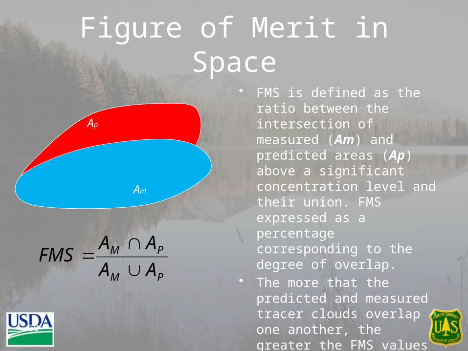
Figure of Merit in Space

• FMS is defined as the ratio between the intersection of measured (Am) and predicted areas (Ap) above a significant concentration level and their union. FMS expressed as a percentage corresponding to the degree of overlap.

• The more that the predicted and measured tracer clouds overlap one another, the greater the FMS values are.

10

Ap

Am

PM

PM

AA

AAFMS

Spatial Statistics• Additional spatial statistics from

Kang et al (2007)– False Alarm Rate (FAR)– Probability of Detection

(POD)– Threat Score (TS)

– A is number of times a condition is forecasted, but not observed (“false alarm”)

– B is number of times a condition is correctly forecasted (“hit”)

– D is number of times a condition was observed but not forecasted (“miss”)

11

100%a

FARa b

100%b

PODb d

100%b

TSa b d

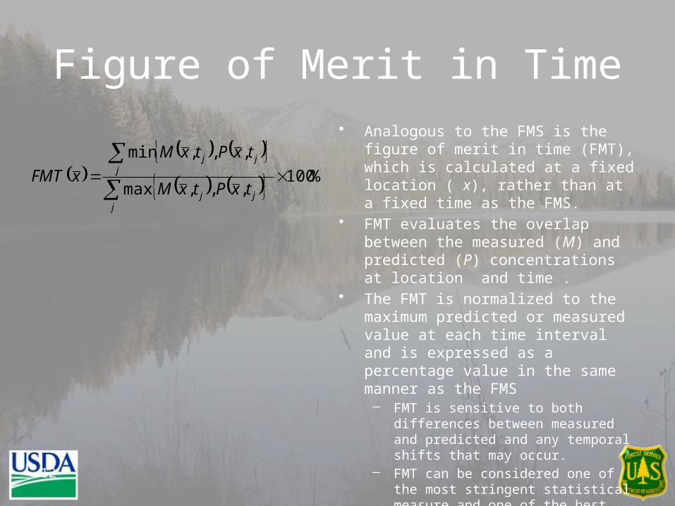
Figure of Merit in Time• Analogous to the FMS is the figure of

merit in time (FMT), which is calculated at a fixed location ( x), rather than at a fixed time as the FMS.

• FMT evaluates the overlap between the measured (M) and predicted (P) concentrations at location and time .

• The FMT is normalized to the maximum predicted or measured value at each time interval and is expressed as a percentage value in the same manner as the FMS– FMT is sensitive to both differences

between measured and predicted and any temporal shifts that may occur.

– FMT can be considered one of the most stringent statistical measure and one of the best overall indicators of the spatiotemporal performance of a modeling platform. 12

%100

,,,max

,,,min

jjj

jjj

txPtxM

txPtxM

xFMT

Model Comparison Parameter

• Draxler et al (2001) introduced a model comparison parameter called RANK, a composite statistic of the four broad statistical categories (scatter, bias, spatial, and unpaired distribution).

• Allows for direct comparison of different models or perturbations in the same model system.

13

1 / 2 /100 1 /100RANK R FB FMS KSP

Evaluation Paradigm• Evaluation procedures follow logic of Chang et al (2003) regarding

multi-model evaluations – Inherent amount of uncertainty due to differences in technical

formulations between various modeling systems– Use common meteorological platform with minimal diagnostic

adjustments to reduce uncertainty• This is a challenge when models such as SCIPUFF and

CALPUFF use diagnostic wind models as primary source of 3-D meteorological data

– Use MM5SCIPUFF developed by Penn State and MMIF (CALPUFF) developed by EPA to couple MM5 directly to these models

– Model control options mostly default “out-of-the-box” configuration• CALPUFF configured for turbulence dispersion and puff-

splitting similar to SCIPUFF, which is a deviation from its default configuration

14

Models Under Evaluation

• Three Distinct Class of Models – Lagrangian Puff Models– Lagrangian Particle Models– Eulerian Grid Models

• CALPUFF Version 5.8 (EPA approved version)• MM5-FLEXPART (Version 6.2)• HYSPLIT (Version 4.8)• SCIPUFF (Version 2.303)• CAMx (Version 5.20)

15

CAMx Configuration• CAMx Version 5.20.1

– 148 x 112 x 25 (36-km)– Inert Tracer, No physical removal– OB70, TKE, ACM2, and CMAQ kv

• OB70, TKE, and ACM2 run with smaller minimum kv than CMAQ option. Potentially leads to differences in dispersive properties among various configurations, especially at night under stable conditions.

• Current version of OB70 option generates unreasonably low diffusion coefficients relative to other options.

– BOTT, PPM advection– Plume-in-Grid (GREASD)/No Plume-in-Grid– Best performance configuration displayed following…

16

European Tracer Experiment (ETEX)

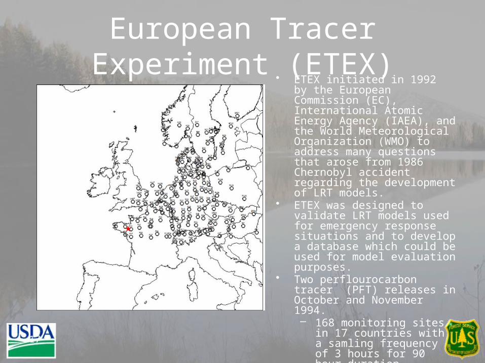
• ETEX initiated in 1992 by the European Commission (EC), International Atomic Energy Agency (IAEA), and the World Meteorological Organization (WMO) to address many questions that arose from 1986 Chernobyl accident regarding the development of LRT models.

• ETEX was designed to validate LRT models used for emergency response situations and to develop a database which could be used for model evaluation purposes.

• Two perflourocarbon tracer (PFT) releases in October and November 1994.– 168 monitoring sites in 17

countries with a samling frequency of 3 hours for 90 hour duration.

17

Meteorology• MM5 Version 3.7.4 used to supply

3-D meteorological fields to LRT models

• Initialized with NNRP dataset (2.5º x 2.5º available at 6h intervals)

• Single 36 km domain, 43 vertical levels

• Physics options– ETA PBL– Kain-Fritsch II Cumulus– RRTM radiation– Dudhia Simple Ice

• Analysis nudging (above PBL for temperature and moisture)

• Performance evaluation against 3-hr observation dataset collected at 168 ETEX monitoring sites

18

ETEX Observed Tracer Pattern

19

Statistical Evaluation• Numerous statistics generated. Focus will be

upon several key statistical parameters which are important to determining performance of LRT model capabilities to predict the timing and direction of pollutant advection:– Figure of Merit in Space (FMS)– Figure of Merit in Time (FMT)

• Model intercomparison metric - RANK

20

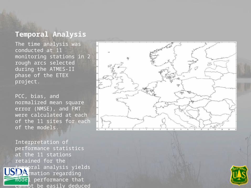
Temporal AnalysisThe time analysis was conducted at 11 monitoring stations in 2 rough arcs selected during the ATMES-II phase of the ETEX project.

PCC, bias, and normalized mean square error (NMSE), and FMT were calculated at each of the 11 sites for each of the models.

Interpretation of performance statistics at the 11 stations retained for the temporal analysis yields information regarding model performance that cannot be easily deduced from the global statistical analysis

21

22

CALPUFF SCIPUFF HYSPLIT FLEXPART CAMx0

10

20

30

40

50

60

FMS

FMS

Figure of Merit in Space(Perfect = 100%)

Figure of Merit in Time(Perfect = 100%)

MODEL RANK(PERFECT = 4.0)

24

CALPUFF SCIPUFF HYSPLIT FLEXPART CAMx0

0.5

1

1.5

2

2.5

RANK

RANK

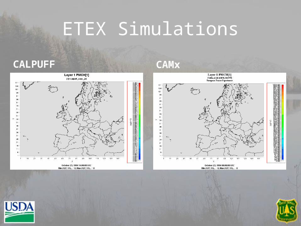
ETEX Simulations

CALPUFF CAMx

25

Summary

• EPA adopted ATMES-II/NOAA DATEM statistical evaluation framework for LRT model evaluations.

• 5 systems currently under evaluation (Lagrangian puff and particle systems, Eulerian Grid Models)

• CAMx has overall best performance for both spatial and global statistical analysis

• HYSPLIT performs best of all competing Lagrangian models examined in this study

• SCIPUFF ranked second, FLEXPART followed closely. CALPUFF lowest performance overall.

26

Acknowledgments

• AJ Deng (Penn State University) – MM5SCIPUFF• Doug Henn and Ian Sykes (Sage) – SCIPUFF guidance• Roland Draxler (NOAA ARL) - HYSPLIT• Petra Siebert (University of Natural Resources – Vienna), Andreas

Stohl (NILU) - FLEXPART• Mesoscale Model Interface (MMIF) Development

– EPA OAQPS– EPA Region 10– US Department of Interior

• US Fish & Wildlife Service Branch of Air Quality• National Park Service Air Division

– US Forest Service Air Resources Management Program

27