evaluation of subsurface fracture geometry using fluid
TRANSCRIPT

V
21107UCID-20156
K>I441
Evaluation of SubsurfaceFracture Geometry Using Fluid
Pressure Response to SolidEarth Tidal Strain
Jonathan M. Hanson,
Manager of Applied Geophysics
Terra Tek Research
Salt Lake City, Utah 84108
September 1984
This is an Informal report Intended primarily for internal or limited externaldistribution. The opinions and conclusions stated are those of the author andmay or may not be those of the Laboratory.Work performed under the auspices of the US. Department of Energy by theLawrence Livermore National Laboratory under Contract W-7405-Eng-48
1, . .: .
K eve- '.
210150224 920914;DR WASTEWM-11 PDR I
- ~Ir

ACKNOWLEDGEMENTS
This report is a summary of work initiated by the author while at the
Earth Science Division of the University of California, Lawrence Livermore
National Laboratory (LLNL) and the subsequent extension of this work while at
Terra Tek Research, Salt Lake City. Funding for the work at LLNL was by the
Department of Geothermal Energy, U.S. Department of Energy. The author would
like to thank Ors. Leland Younker and Paul Kasameyer, LLNL, and Ors. John
Schatz and Lawrence Owen, Terra Tek Research, for their many helpful comments
during the course of this work. I would also like to thank Anne MacLeod of
Terra Tek Research for her patience in typing this manuscript.
�-- -:- !t .

TABLE OF CONTENTS
Page
List of Figures. . ........ .... . i.
List of Tables. . . . . . . . . . . . ... . . . . . . . . . . . . . vii
Chapter I - Introduction. . . . . . . . . . . . . . . . . . . . . . 1
Chapter II - Nature of Solid Earth Tidal Strain and SurfaceLoad Deformation. . . . . . . . . . . . . . . . . . . . 5
Chapter III - Pore Pressure Response to Tidal Strain and SurfaceLoads . ........................ 17
j Chapter IV - Integration of Tidal Response with Conventional PumpTests for Fracture Characterization . . . . . . . . . . 41
; Chapter V - Spectral Analysis, Correlation, and Error Estimation. . 59
Chapter VI - Case Study - Raft River Geothermal Area . . . . . . . . 71
Chapter VII -Summary and Conclusions . . . . . . . . . . . . . . . 121

I
LIST OF FIGURES I
IiIIII
II
Fioure
2.1
2.2
2.3
3.1
3.2
4.la
4.lb
4.2a
4. 2b
Title
The Main Lines of the Spectrum of the Tidal Potential . .
Amplitude Variation of the Principal Tidal Constituentsas a Function of Latitude for the Vertical Component ofGravity . . . . . . . . . . . . . . . . . . . . . . . . .
Distribution of Tidal Deformation Amplitudes as aFunction of Azimuth and Dip for the 01 and M2 Tides . . .
Amplitude and Phase Response of a Confined HomogeneousIsotropic Aquifer Penetrated by a Well. . . . . . .
. @
0
Page
6
. -
4.2c
4.3a
4.3b
4.4a
4. 4b
4.4c
5.1
Finite Vertical Bi-Wing Fracture Model and FinitePenny-Shaped Fracture Model . . . . ... . . . . . . .
Pressure History During a Drawdown-Buildup PressureTransient Test. . . . . . . . . . . . . . . . . . . .
Time Derivative of Data Shown in Figure 4.1a. . . . .
Linear Formation Flow Constraint Given in Equation (I
Bilinear Flow Constraint After Shut-In Given byEquation (IV.8c). . . . . . . . . . . . . . . . . . .
Bilinear Flow Constraint Before Shut-In Given byEquation (IV.8b). . . . . . . . . . . . . . . . . . .
Pressure History During a Orawdown-Buildup PressureTransient Test . . . . . . . . . . . . . . . . . . .
Time Derivative of Data Shown in Figure 4.3a. . . . .
Linear Formation Flow Constraint Given in Equation (I
Bilinear Flow Constraint After Shut-In Given byEquation (IV.8c). . . . . . . . . . . . . . . . . . .
Bilinear Flow Constraint Before Shut-In Given byEquation (IV.8b). . . . . . . . . . . . . . . . . . .
Example of Uncertainty Error Ellipse of a TidalConstituent in the Complex Plane. . . . . . . . . . .
Flow Chart Showing the Various Stages of Tidal DataProcessing and Analysis . . . . . . . . . . . . . . .
V.8a).
. . .
10
12
22
30
48
49
SO
51
52
53
54
55IV. 8a).
56
57
67
5.268

List of
f igou-e
6.1
6.2
6.3
6.4
6.5
6.6
6.7
6.8
6.9
6.10
6.11
6.12
6.13
6.14
6.'15
6.16
6. 17
6.18
Figures (continued)
Title
Raft River Valley and Major Structural FeaturesAdjoining the Valley . . . . . . . . . . . . . . . .
Cross-Section 9-BI of Figure 6.1. . . . . . . . . . . . . .
Geothermal Well Locations Within the Raft River Geo-thermal Field ......... . . ............
Raft River Geothermal Wells, Showing Casing Depths..
Raw Downhole Pressure Data at RRGE-1. . . . . .. . .
Raw Downhole Pressure Data at RRGE-2. . . . . . . . .
Raw Wellhead Pressure Data at RRGE-3. . . . . . . . .
Raw Wellhead Pressure Data at RRGE-4 Shoving Pulse test . .
Raw Wellhead Pressure Data at RRGI-6. . . . . . . . . . . .
Raw Wellhead Pressure Data at RRGI-7. . . . . . . . . . . .
Raw Welihead Pressure Data at RRGI-7. . . . . ..
Conuted Barometric Efficiencies for the Raft RiverGeothermal Field. . . . . . . . . . . . . . . . . . . . . .
Barometric Pressure Recorded at Pocatello, Idaho andMeasured Pressure Response to Barometric Loacinc Dividecby Barometric Efficiency, RRG-1.. . . . . . .. .
Barometric Pressure Recorded at Pocatello, Idaho andMeasured Pressure Response to Barometric Loading Dividedby Barometric Efficiency, RRGE-2. . . . . . . . . . . . . .
Barometric Pressure Recorded at Pocatello, Idaho andMeasured Pressure Response to Barometric Loading Dividedby Barometric Efficiency, RRGE-3. . . . . . . . . . . . .
Baiometric Pressure Recorded at Pocatello, Idaho andMetsured Pressure Response to Barometric Loading Dividedby Barometric Efficiency, RRGE-4. . . . . . . .. .
Barometric Pressure Recorded at Pocatello, Idaho andMeasured Pressure Response to Berometric Loading Dividedby Barometric Efficiency, RRGE-6.... ..........
Earometric Pressure Recorded at Pocatello, Idaho ancMeasured Pressure Response to Barometric Loading Divioedby EBrometric Efficiency, RRGI-7(a) . . . . . . . . . . . .
iv
List
Paoe
73 6-:
746..~
75
76
77
78
79
80
81
82
83
6.
6.
6.
6
6
E
esI
85
87
88
89
- -_P-�_ .. - -- . -_ . - __ -

!I'I
'List of Fi
Pace ;Figure
. . 73 {6.19
. . 74 I
4 6.20
75
76 i 6.21
* 77 178 i6.22
* 16.23
gures (continued)
Barometric PressuiMeasured Pressureby Barometric Eff'
Title
re Recorded at Pocatello, Idaho andResponse to Barometric Loading Dividediciency,RRGI-7(b).. ....... I
* so
laI
82 If85 J86
6.24
6.25
6.26
6.27
6.28
6.29
6.30
6.31
6.32
6.33
6.34
Isolated Welihead Pressure Response to Tidal Strain atRRGE-2, Showing Theoretical Tidal Gravity Over SameTime Period .. .... . . . . . . . .....
Fourier Amplitude Spectrum Based on Finite FourierTransform, RRGE-1 . . . . . . . . . . . . . . . . . . .
Fourier Amplitude Spectrum Based on Finite FourierTransform, RRGE-2 . . . . . . . . . . . . . . . . . . .
Fourier Amplitude Spectrum Based on Finite FourierTransform, RRGE-3. ..................
Fourier Amplitude Spectrum Based on Finite FourierTransform ,RRGE-4 . .................
Fourier Amplitude Spectrum Based on Finite FourierTransform, RRGI-6. ..................
Fourier Amplitude Spectrum Based on Finite FourierTransform, RRGI-7(a) . . . . . . . . . . . . . .
Fourier Amplitude Spectrum Based on Finite FourierTransform, RRGI-7(b).. ...............
Computed Tidal Admittance Showing 90% Confidence Inter-vals, RRGE-1. . . . . . . . . . . . . . . . . . . . . .
Computed Phase Shift Showing 90% Confidence Intervals,RRGE-1. . . . . . . . . . . . . . . . . . . . . . . . .
Computed Tidal Admittance Showing 90% Confidence Inter-vals, RRGE-2 . ....................
Computed Phase Shift Showing 90% Confidence Intervals,RRGE-2. ........................
Computed Tidal Admittance Showing 90% Confidence Inter-vals, RRGE-3. . . . . . . . . . . . . . . . . . . . . .
Computed Phase Shift Showing 90% Confidence Intervals,RRGE-2. ........................
Comouted Tidal Admittance Showing 90% Confidence Inter-vals, RRGI-6. . . . . . . . . . . . . . . . . . . . . .
.
.
99
100
101
92
93
94
95
96
97
98
87
88
89
90
aseO
102
103
104
105
106
107

List of Figures (continued)
Ficure Title ftae
6.35 Computed Pnase Shift Showing 90% Confidence Intervals,RRGI-6. 6. ........................ 108 T 9
K..> 6.36 Computed Tidal Admittance Showing 90% Confidence Inter- 3vals, RRGI-7(a) . . . . . . . . . . . . . . . . . . . . . . 109 6
6.37 Computed Phase Shift Showing 90% Confidence Intervals,RRGI-7(a).. . ........... 110 I
6.38 Computed Tidal Admittance Showing 90% Confidence Inter-vals, RRGI-7(b) . . . . . . . . . 0 0 .. . . . . .111
6.39 Computed Phase Shift Showing 90% Confidence Intervals,RRGI-7(b) ... . . 112
6.40 Computed Fracture Zone Strike for RRGE-1, 2 and 3 Showing90% Confidence Strike Sectors . . . . . . . . . . . . . . . 118
6.41 Histogram of Dip Angles of Fractures in Core Taken atRRGE-1 and RRGE-5 ............ 119
7.1 Measured Welihead Pressure at a Stimulated Well in aWestern Canadian Oil Field. . . . . . . . . . . . . . . . . 128
7.2 Maximum Entropy Amplitude Spectrum of a Portion of theData Shown in Figure 7.1. . . . . . . . . . . . . . . . . . 129
vi

_" k A'A ~ m~r- - * --L ~ 4ArAC.'.rV %stkCi. =l ~-pAt' .. ~."' 2- t~l - i '"'7 i~iA.. -
I~~~~~~~~~~~~~~~~~~~~~~~~~~~~~~~~~~~~~~~~~~~~~~~~~~~~~LIST OF TABLES
Page-
. .
108 ! TableI
i 3.1
1091.lo10 6.1
1
112
Title Page
Frequencies of Major Tidal Constituents . . . . . . . . . . 27
Summary of Computed Specific Storage and Porosity Valuesfor the Raft River Gethermal Field. . . . . . . . . . . . . 114
Radioactive Waste Containment Tests - Chalk River NuclearLaboratories, Ontario, Canada, 1982 - Borehole CR8* . . . . 122
g. . 118
* 119
. 128
* 129
i
i
p

iI
CHAPTER I
INTRODUCTION
I
The development of high-temperature, liquid-dominated geothermal resour-
4 ces will require the production and ultimate disposal of large volumes of
fluids. Subsurface injection of the wastewater is the only environmentally
acceptable scheme for disposal of most geothermal waters primarily because of
moderate to high concentrations of dissolved salts. Relatively high waste
water rejection temperatures and large discharge volumes also require subsur-
face disposal. The feasibility for long-term, large volume reinjection of
sDent geothermal fluid in the United States has yet to be established.
One critical area of concern is the movement and effects of the fluids as
they enter the subsurface formation. In order to insure that the objectives
of an injection program are realized without undue risk of environmental
deterioration, a method to predict and monitor the movement of the injected
fluid is necessary. Numerous case studies have demonstrated that the major
uncertainty associated with attempts to predict the movement of injected fluid
is the presence and orientation of fractures. High permeability fracture
Zones can serve as conduits for injected fluid and can channelize fluid move-
ment in a localized and unpredictable fashion. Development of monitoring
approaches which allow major fluid carrying fractures to be mapped and charac-
terized would help to guarantee successful long-term reinjection programs.
Careful measurement and interpretation of pore pressure response to solid
earth tides has the possibility of identifying the nature and orientation of
the primary fluid conduits away from the Injection well. This information
would be useful in developing flow models that accurately predict behavior of
Spent fluids in the injection zone. The appeal of this approach is that no'� S� . JI I
4

tec n u s capable of mapping fracture orientation at
depths below a few thousand feet. The target parameters for tidal reservoir Jo.
testing are the same as conventional testing. However, because the- driving Or
forces are directional (tidal strains are tensors), the spatial orientation,,_>ie
the preferred flow conduits will be manifested in the well pressure record. nos
Preliminary work done by The University of California Lawrence Livermore
National Laboratory (LLNL) on data taken at the Raft River Geothermal Area thi
indicates that the nature of connected (i.e., pore or fracture) porosity and ant
fracture orientation can be estimated from the analysis of pore pressure bat
response to solid earth tidal strain. pro
Subsequent work by Terra Tek Research (Salt Lake City, Utah), has ex- cot
tended the theory to allow for the more complex situation in which drainage to a
and from the fracture to the formation takes place. Terra Tek Research has th,
successfully field tested this approach in a hydraulically stimulated oil well un
in an active western Canadian oil field located adjacent to the Eastern Rocky fil
Mountain thrust belt (Hanson, 1982). In addition to work done at LLNL an, me
Terra Tek Research, an effort is currently underway by the Oepartment of in
Energy, Mines, and Resources, Canada, to investigate the feasibility of char- to
acterization of isolated natural fractures in deep crystalline rock masses s)
using the solid earth tidal strain approach (Bower, 1982). This investigation VI
is directed toward the subsurface containment of radioactive wastes. ml
It is clear from the above that fracture orientation evaluation using r
fluid pressure response to solid earth tidal strain has applications in a e
diverse set of field situations. The rapid development of the method over the
past few years derives primarily from the development of the extremely high
precision quartz pressure gauge and improvements in numerical data analysis
methods for extraction of the small pressure signals in background noise. The
2'4/1

'rtatioh at esults of the work carried out by LLNL at the Raft River Geothermal Reservoir
reservoir in Idaho and subsequent work by Terra Tek Research in field-testing the method
e driving for fracture orientation analysis in a stimulated oil well has been suffi-
itation of ciently encouraging to permit Terra Tek Research to offer this fracture diag-
e record. nostic method as a commercial service.
Livermore The purpose of this report is to describe in detail the current state of
rnal Area this technology. Chapter II discusses the nature of solid earth tidal strain
Osity and and surface load deformation due to the influence of gravitational forces and
pressure
has ex-
inage to
irch has
Oil well
'\< Rocky
.NL and
ent of
char-
masses
gation
using
in a
r the
high
lysis
\,,. The
barometric pressure loading. Chapter III investigates in detail the pore
pressure response to these types of deformation, including the cases of a
confined aquifer intersected by a well and a discrete fracture intersected by
a well. For the case in which the fracture intersects a permeable formation,
I the solution for the fracture orientation is under-determined. That is,
unless the formation hydraulic parameters are known a priori, there is insuf-
ficient information to calculate the fracture orientation based on simply the
measurement of fluid pressure to tidal strain. Chapter IV discusses the
integration of the tidal response method with conventional pump tests in order
to independently calculate the hydraulic parameters of the fracture-formation
system. With this information available, the solution for fracture orienta-
tion is again over-determined. Chapter V shows how advanced spectral analysis
methods, coupled with correlation analysis can be used to extract the tidal
response signals from the pressure record. Uncertainties in the signals are
estimated using various information-theoretic methods in order to place a
confidence level at which we can safely assume that the measured signal is
indeed of tidal origin. Chapter VI presents a detailed case study of the
method carried out at the Raft River :eothermal Reservoir in Idaho. This study
details the background geology and geophysics of the area and summarizes the
. . - -0 - _ _ . - 2*-- - !t�-

current understanding of the geothermal system. All of the analyzed tic
data is presented and the results of the computed fracture orientation usir,
the solid earth tidal strain approach are compared with the extensive fip-
work carried out at Raft River by the Department of Geothermal Energy (U. 's-"surn
DOE) over the past decade. Chapter VII discusses the direction that futur.due
work in the continuing development of this technology should take, including
1) the present need for an expanded data base for the confirmation of presen'loCi
tidal strain response models, and 2) improvement in response models.Var
the
cOn
ete
las
the
ete
is
', dev
(1l
se'
re
di
Mf
t
g
. Z�=-
- '- - -- -
4

- -IQ.st,"'-t±'
CHAPTER IIlyzed tide!
< , on NATURE OF SOLID EARTH TIDAL STRAIN AND SURFACE LOAD DEFORMATIONs ation usir.
insive fiellSolid earth tidal strain is a global phenomenon. Every point on the
nerMy (U.SIIsurface and within the earth is subject to two forces: the force of gravity
that futureIdue to Newtonian attraction of the mass of the Earth, Moon, and Sun, and the
icluding, centrifugal force due to the rotation of the earth. Because the relativeof presen
location of the Moon and Sun with respect to a fixed point within the earth
varies with time, the forces at that point will also vary with time and with
I the orbital paths of these bodies. The tidal gravitational potential, and
consequently the tidal force, can be evaluated if the various orbital param-
eters are known. Taking advantage of the work performed by astronomers of the
g last century, it has been possible to determine with extraordinary precision
tnese orbital parameters. A description of the method by which these param-
eters are translated into an expression for the tidal gravitational potential
is beyond the scope of this report. However, a detailed description of this
development is given by Melchior (1966, 1978), Longman (1959), and Harrison
(1971). The tidal spectrum is not a simple distribution. Because of the
several gravitational periodicites involved, corresponding to rotational and
revolutional periodicities, the major tidal energy bands (i.e. diurnal, semi-
Oiurnal, etc.) are broken down into a complex, but well understood, *fine
Structure". Figure 2.1 shows the main spectral lines of the tidal potential.
Melchior (1966) points out that, although the total number of lines in the
tidal spectrum is quite large, only five of the lines have real importance
.eophysically. These five are the two diurnal tides (01, K1) and the three
seMi-diurnal tides (N2 , M2 , and S2).
I' the Earth was an ideally rigid body, then these applied gravitational
forces Would_4ngYce nqdeformation. iHowever, the Earth is not rigid, but

---I
I ,i i
It I It
: II
1.0
0.8
0.8
IFl ir
an
if'
&r
HI
elJ
Zt(j)
0.4
0.2
-a. CYCLES4 PER DAY0 1 2 3
Cal
Figure 2.1. The main lines of the spectrum of the tidal potential (fromGodin, 1972). p
a
6

9 - I., 2 Pk"~~~~~~~~~~~~~*** U l ~'iiii.dtE'~wuimrir'~-
behaves as an elastic-viscoplastic body with complex rheological behavior.
for our present purpose, the Earth can be considered to behave in a purely
inear-elastic (Hookean) manner to good first approximation. Because of the
non-rigid nature of the Earth, gravitational forces will cause strain deforma-
tion -- both cubic expansion and shear. In order to quantify the magnitude of
these deformations, a knowledge of the distribution of density p and elastic
Lamd parameters X and p from the center of the Earth to the surface is re-
quired. This information can be estimated from tabulated seismic velocity
data for P and S waves. Sources of this data are given by the Jeffreys-Bullen
and Gutenberg-Sullen models (Bullen, 1975). Takeuchi (1950) was the first to
; integrate this data to obtain the theoretical deformation characteristics of
%the Earth under applied gravitational forces. His calculations assumed a
Hookean Earth. The results can be easily expressed in terms of three param-
eters: the Love numbers h and k and the Shida number e. These three param-
.ES eters allow a very practical representation of all deformation phenomenaDAY
Produced by a gravitational potential. The various theoretical tidal strain
tensor components are simply linear combinations of the tidal gravitational
from Potential and its spatial derivatives. The coefficients of the linear combin-
ations are the Love and Shida numbers. Further details can be found in Mel-
Chior (1966, 1978). The desired result obtained by combining the elastic
Parameters of the Earth (i.e. the Love and Shida numbers) and the tidal gravi-
tational potential is the tidal strain tensor c(t) which is a function of
time E(t) is represented as:
e(t) = ek eA(t) he X6tt)tIl
, ~ ~ ~~~~~~~O he 1\t) e66(t)J
4 i. ._ ..

where err, el, and e8 are tidal strains in the radial, E-W, and N-S dire
tions, respectively. e~8 is the shear strain in a plane tangent to the earthe
surface. It should also be pointed out that the strain tensor componr
depend on location (latitude and longitude) at the Earth's surface.
The depth range of interest, namely a few to tens of kilometers, is muc
less than the wavelengths of the tidal strain. Therefore, to very good approxi z
imation, measurements to these depths can be considered measurements at a fre1
surface (Melchoir, 1978). Therefore, e~r = er = 0, as reflected in the for; '
of the tidal strain tensor. The cubic dilatation a, which will be useful inQ
the discussion of pore pressure response in isotropic homogeneous porous rock,
is given by the trace of the strain tensor, namely:
jt
A(t) = err(t) + e,,(t) + eea(t) (II.2)
Since the tidal strain can be represented as a finite sum of constituents,
each of which exists at a specific frequency, it is appropriate to recast the
strain tensor into its Fourier components. Each tidal constituent (e.g. L,_J
K1, N2, M2, or S2) is represented by a strain tensor cast in the frequency
domain,
[rr(wk) 0 o ( ]
t(wk) - o &a(wk) h(wk) (II.3)
O re~fXs k) '80(wk)J
k = 1, 2, ... , N
where the index k corresponds to a particular frequency (i.e. tidal constitu-
ent).
The following numerical exercise is presented in order to get a feeling
for the magnitude of the volumetric tidal strain at the Earth's surface. As
a

N-S di, eicnior (1978) points out, a can be cast as a function of the Love and Shida
numers h and I and Poisson's ratio v as:
a = 1-iV (2h - 61) W?r__V ~~ag(11.4)
S, is mUX
at a fre
1 the for
useful ii
Ous rock,
where a is the radius of the Earth, W2 is the tidal potential, and g is the
acceleration of gravity (not tidal) due to the Earth's mass. Taking Takeuchi's
values of h, and A, and noting that the tidal gravity perturbation Ag is given
by (Melchior, 1978):
a
(II.2)
ituents,
> ~st the
!. g. 1 I
equency
:I.3)
Stitu-
!eling
AsI'e
I
V
I'hen
I ,i
I
1 = .1-V (2 h - 6 U) g (II. 5)
FrI
trI
= 0 49 2- ~~2g
where Poisson's ratio has been taken to be V = 0.25 and h, I are 0.606 and
0.082, respectively. Figure 2.2 shows the variation of Ag for the major tidal
Constituents as a function of latitude. It is noted that
1 pgal = xlO-6 cm/sec2
g = 980 cm/sec2
Therefore, using the above expression for tidal cubic expansion, the K2-tide
has a maximum volumetric strain of:
(O. 49)80x10-6)N2= (2)(980)
2x10-$
I is clear from the above exercise that tidal strains are exceedingly small.
_ - -o. - ~ - - - . - -k - - -

Oal
-IAi
ri!
Xe e~~~~~~~X*- I I ,-:- S ! s
0*} 4 . _ 0*w~
$ >rc
CD~~~~~~~~~~~~~~~~~~~~~~~~~~~~~~~~~~~~~~~~~~~~~~~
Figure 2.2. Amplitude variation of the principal tidal constituents as afunction of latitude for the vertical component of gravity (from.. thiMelchior, 1978).
As
th
de
ol
C1
a
M
10

Because strain is a tensor quantity, tida1 deformation will depend upon
Spatial direction. The best way to see this is to evaluate the strain quadric.
This is accomplished by evaluating the strain amplitude 6n along a given
direction in space defined by the unit vector n, where
. n = (Cosal, Cosa2, Cosa3)T
Cosa1 , Cosa2 , Cosa3 are the direction cosines between n and the (vertical,
E) coordinates, respectively. Thus,
6n =G t (I.6)
O , upon multiplication:
a = Cos2a, err + Cos2a2 e + Cos 2a3 ea + Cosa2 Cosa3 e8a
Figure 2.3 shows horizontal and vertical slices through the quadratic
Surface for the 01 and M2 strain tensors evaluated at a latitude of 450. The
q uadric surfaces have been normalized so that W2/(ag) = 1. It is clear that
f'mm this figure that the 01 tide has a distinctly different deformation
distribution than the M2 tide. The maximum deformation for the M2 tide is in
sY from N-S direction whereas the maximum for the a1 tide is in the E-W direction.
As will be seen in a later chapter, this will play a major role in determining
the spatial orientation of a fluid-filled fracture.
Deviations of the measured tidal strain from the theoretical strain
determined from radially stratified earth models mentioned above come about
through a variety of reasons. The most important of those are: 1) the effect
Of loading due to ocean tides, 2) local geologic inhomogeneities and/or dis-
Continuities in the elastic parameters near the region of strain measurement,
and 3) topographic effects. The observed deviations, and various attempts to
%Odel them, have been documented by many authors, including Beaumont and

t1-AVO."
r (01
N RaN~~~~~~~~~~~~~~~~~N)
%I~~~~~~~~~~~~~~~~~~~~~~~~~~~~~~~~~~
w L~~~I -
I% WA,"
O TIDEM 2 TIDE
Figure 2.3. Distribution of tidal deformation amplitudes as a function of
azimuth and dip for the 01 and M tides (from Melchior, 1978).
i '
12a&-~~~~~~~~~~~~~~~~~~~
.-

l
Berger (1975), Berger and Beaumont (1976), Alsop and Kuo (1964), Harrison
(1976), Prothero and Goodkind (1972), Harrison, et al. (1963), Lambert (1970),
Berger and Wyatt (1973), Farrell (1972, 1979), King and Bilham (1973), and
Kuo, et al. (1970). The results of these investigations can be summarized as
fol lows.
in..
N-- ..
I/F
r
-S
1. The effect of loading due to ocean tides can be significant -- up to
44 percent of the total tidal strain tide for the K2 constituent and
13 percent of the total tidal strain for the 01 constituent (Beau-
mont and Berger, 1975). These extreme variations are found near
coastlines where the loading effect is most significant, and in most
cases, diminish to a second-order effect a few hundred kilometers
inland. If cotidal and cophase charts are available for the oceans
adjacent to the nearest coastline, the loading effect can be approx-
imated and therefore removed from the observed strain tide.
2. Geologic effects are theoretically important near interfaces between
rock types that have radically differing elastic properties. As
Berger and Beaumont (1976) point out, "it is difficult to make
general statements on the effects of lateral variations in the
crust's elastic properties due to geology on the local strain field.
This results not so much from a lack of mathematical tools to solve
the problem as from the uncertainty in the three-dimensional struc-
ture. Were these local variations better known, finite element
models could readily be constructed to estimate their effects."
Topographic and geologic effects at some strain meter sites have
been found to be as large as 25 percent of strain calculated from
the radially-stratified whole earth model. Typically topographic
effects are considerably smaller than geologic effects. In the case
on of1978).
L
rr

of geologic effects, however, the spatial variations in the elast c
parameters will be a necessary input to a model for tidal strain. -
Berger and Beamont (1976) have carried out such an analysis at-
several sites using relatively simple representations of local I
variations in elastic parameters obtained from regional geology and
seismic surveys. This kind of information is often times typically!
available for geothermal and petroleum reservoirs. Berger and;
Beaumont's modeling results were consistent with the measured tidal; &cc
strains. If this kind of site-specific information is not availablei
an estimate of the uncertainty in elastic parameter anisotropy must!
be made before the effect of geology on the uncertainty in derived bar
fracture orientation can be evaluated. Clearly more work needs to Dar
be done regarding the effect of local geology on the evaluation off Coe
fracture geometry using solid earth tidal strain. flu
estIt is noteworthy that none of the above investigations of anomalous tidal
notstrain have included the effects of lcadirg due to barometric pressure. There,__,j
is considerable evidence in the literature to indicate that variations in
barometric pressure can induce measureable ground deformation (Tanaka, 1968 a,
b; Trubytsyn and Makalkin, 1976; Khorosheva, 1958; Urmantsev, 1970, 1975; and
Zschau, 1976). Tanaka (1968 a) found that the ground strain response at Oura,
Japan due to atmospheric loading was roughly lx10-8/mb in the N-S direction
and 2.5x10- 8 /mb in the E-W direction for loading periods between 5 minutes and
60. minutes. Chapman and Westfold (1956) report barometric loads at tidal
frequencies ranging from 2.8 to 91 pb for the M2 tide and 208 to 1482 pb for
the S2 tide. We have measured barometric loads at tidal frequencies computed
over a two month period at the Imperial Valley in Southern California, of 18.3
pb, 1358.4 .ub, 14.5 pb, 82.3 pb, and 829.7 pb corresponding tc the 01, K1, N2,
.4
I M

1~ J
CHAPTER III
PORE PRESSURE RESPONSE TO TIDAL STRAIN AND SURFACE LOADS
Many examples of pore pressure response to solid earth tidal strain and
barometric pressure loading have been documented in the literature (Robinson,
1939; Richardson, 1956; Robinson and Bell, 1971; Bredehoeft, 1967; Sterling
and Smets, 1971; Marine, 1975; George and Romberg, 1951; Arditty and Ramey,
1978; Bower and Heaton, 1978; Witherspoon, et al., 1978; Rhoads, 1976; Kane-L~~~~~~~~~~~~~' no:
hiro, 1980; Hanson, 1979; Hanson and Owen, 1982; and Bower, 1982). Models
used to interpret the fluid pressure data are typically based on the theoreti-
Cal response of a homogeneous isotropic fluid-filled porous elastic rock
(Arditty, 1978; Bodvarsson, 1970; Moreland, 1978; Bodvarsson and Hanson, 1978;
Bredehoeft, 1967; Van der Kamp and Gale, 1983). Most of the models do not
include: a) borehole storage and well-completion effects, and/or b) the
presence of discrete fluid-carrying fractures. In the following, we present
tWO models for pressure response to solid earth tidal strain. The firsttl '
todel, based on Biot's theory of consolidation, is similar to previously
Published models for aquifer response to tidal strain. It is presented here
Primarily for completeness and will be used later for interpretation of data
from the Raft River Geothermal Reservoir. The second model addresses the
question of fluid pressure response in a single discrete fracture. Both
models include the effects of borehole storage and welihead completion.
A. Homogeneous Isotrooic Aouifer Response to Solid Earth Tidal Strainand Barometric Loads
Consider a confined single-phase fluid-filled aquifer of thickness L,
Permeability k, and porosity +, subject to an applied volumetric tidaY strain
k

- -WISSAMOM
le elastic
I Strain.
lysis at
of local
31ogy and
:ypical ly
-ger and
ed tidal
vailable,
Opy must
derived
eeds to
tion of
tidal
There
ins in
968 a,
3; and
Oura,
ction
s and
tidal
3 for
iuted
18.3
N2 ,
Y2, and S2 constituents. Thus, barometric pressure induced strain, based on
COapman and Westfold's barometric load amplitudes and Tanaka's response " s
say be as high as 3.71x10⁻³ for the S2 tide and 0.23x10-$ for the 12 tide.
Using our barometric loads measured at the Imperial Valley, we obtain baro
metric pressure induced strains of 4.6x10⁻¹⁰, 3.4x10⁻⁸, 3.6x10⁻¹⁰, 2.05xl0-9,
and 2.07x10-$ corresponding to the 01, K1, N2, M2, and S2 tides, respectively.(
It is evident from the above that the effect of barometric loads must be
,aCcounted for in addressing the question of deviations in tidal strain fro
its theoretical value.L
For the purposes of this report, we have accounted for the effect of
Barometric loading on strain by finding the correlation coefficient between
Barometric pressure and pore fluid pressure. Having obtained the correlation
Coefficient, the effect of barometric loads can easily be removed from the
fluid pressure data. This approach circumvents the intermediate str 'f
Estimating barometric pressure-induced strain, since for this report w S renot particularly interested in this parameter. The correlation method will be
discussed elsewhere in this report (see Chapter V).
I.. .
It r.I'
5
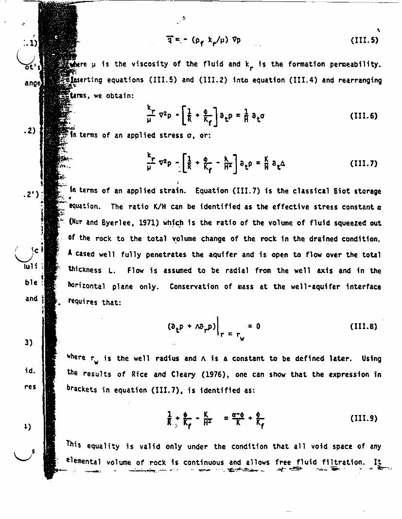
% t- (pf kr/p) Vp (III.5)
ere p is the viscosity of the fluid and kr is the formation permeability.
ang> Ierting equations (III.5) and (III.2) into equation (III.4) and rearranging
tems, we obtain:
ir V2P' + atL p= aBa (III.6)
.2) In terms of an applied stress a, or:
r~~~~~~
kr V2p F 41+- K R a tP K t (III.7)p ~~~L~Kf HtP~
in terms of an applied strain. Equation (III.7) is the classical Biot storage
equation. The ratio K/H can be identified as the effective stress constant a
(Nur and Byerlee, 1971) which is the ratio of the volume of fluid squeezed out
Of the rock to the total volume change of the rock in the drained condition.
A cased well fully penetrates the aquifer and is open to flow over the total
lu iluli thickness L. Flow is assumed to be radial from the well axis and in the
ble horizontal plane only. Conservation of mass at the well-aquifer interface
and requires that:
(Stp +ArP) 1|. rw = 0 (1II.8)
3) i
where r is the well radius and A is a constant to be defined later. Usingw
id. the results of Rice and Cleary (1976), one can show that the expression in
res brackets in equation (III.7), is identified as:
$) X + t - F = t~~~ + K (III.9)
This equality is valid only under the condition that all void space of any
elemental volume of rock is continuous and allows free fluid filtration. It

err 8 AX Iwhere err + eea + eAX is the trace of the tidal strain tensor. Using Bfotts|
(1941) linearized theory of consolidation, the volumetric strain a and chant
in pore volume fraction 8 can be written as:
! (111.2)
with the inverse relationship:
/ D
p(a,8) = [g- I] D (11.2
where D = (KR) - H 2
and where p is the change in pore pressure, a is the change in hydrostatic
stress, K is the drained wet rock bulk modulus, and H, R are elastic moduli
defined by Biot (1941). Assuming that the fluid is only slightly compres iib
so that the mass of fluid per unit pore volume is a linear function of a and
p, the change of fluid mass per unit volume can be expressed as:
m = Pf [3 + (III.3)
where pf, Kf are the density and bulk modulus, respectively, of the fluid.
Conservation of fluid mass within an elemental volume of the aquifer requires
that:
at M + V- = 0 (III.4)
where q is the mass flux through the surface of the volume, given by Darcy's
law:
18

N I I q4
966) of tn Kg sugh that a > 0.9, and to good approximation a ~ 1 is sufficient for
the current work. With the'help of equation (III.11), we can rewrite equation
K.-> (III.7) as:'II. lo
bracken ~~~~~kr v2p _ Ss atp = caahtl.'
cient. Assuming an oscillating volumetric strain field of the form a = &a exp (iwt),
equation (II1.7') along with the boundary condition given by equation (III.8)
can be solved in cylindrical. coordinates to obtain:
pIjrr a aPfg T . (III.13)
ghere T is a function given by:
iA rw KI(Xrw)T = o(Arw) (II.14)
and where
0 o. As = (III.15)Pfgkr
rage,
1.11) The constant A, which is determined by the well completion, is easily shown to
be: z *-! .
2gpf-| krLo open well with free liquid surface
A ~
the - f k L. shut-in well with positive
the 7e L* is the depth ~.ir i r' wellhead pressure
h is the depth of the well. The function T/(l+T) has been evaluated
the numerically for its amplitude and phase characteristics. Figure 3.1 shows
ort. these results in terms of three-dimensional surfaces for dimensionless pres-
ss tSure amplitude and phase in terms of the dimensionless parameters A/(wry)
*Gnd Xrw . It is noted that X 1 can be interpreted ask a hydraulic skin

is useful to compare equation (111.9) with the definition (DeWeist, 1966) oi
specific storage S5 of a homogeneous isotropic aquifer:
S5 v + ° lIlpfg~~~~~
where g is the acceleration of gravity. We see that the expression in brack
ets in equation (III.7) closely resembles the specific storage coefficient.
Indeed, setting a 1 obtains:
I + o K SS
We suggest here that a more realistic expression for the specific storage
coefficient is given by:
55 (111 (I.11)
This is based on taking the limit of equations (III.10) and (III.11) as -
Equation (III.10) implies that a rock with zero porosity has a finite storage,,
which is clearly a non-physical result. On the other hand, equation (III.11):
has a limiting specific storage of
s a (III. 12)pfg K
as 0 * 0. Noting that (Nur and Byerlee, 1971) a = 1 - K/KgI where K Is the
grain modulus of the rock, as 0, K * K and hence a 0. ThusW the
specific storage given by equation (III.11) goes to zero as 0, which is
the desired physical result. We will therefore use equation (III.11) as the
definition of specific storage coefficient in the remainder of this report.
We point out here that for many, if not most, rocks, K is sufficiently less
20
A I I

depth, or in terms of conventional well testing, a "radius of influence." It
is clear from Figure 3. 1that, for A/(wrw) > 100, the fluid pressure oscil-
lates in phase with the applied volumetric strain, with pressure amplitude
given as:
f ~~~~~~~~c apfgP¶-= - ho (III.16)
For A/(wr ) < 100, the pressure response falls off with decreasing A and also* * ~~w
exhibits a phase lag (vIjth, respect to aO) that can be as large as 900. To
good approximation, equation (II1.16) holds if the permeability-thickness
product of the aquifer is:
{ 2.4x10⁴ md-ft, open well
krL 10.4x10⁻³LV md-ft, closed well, positive well-head pressure (L* in feet)
where we have assumed rw = 0.1 m, p = 1 cp, Kf = 2.3x1O9 Pa, and pf = 103
kg/m3.
The weight of the atmosphere pressing on a confined aquifer will cause a
Pore deformation and consequently a pore pressure change. The ratio of the
Pore pressure change to the atmospheric pressure change is referred to as the
"barometric efficiency' o the reservoir. Jacob (1940) was the first to show
the relationship between the barometric efficiency and the specific storage
for a porous aquifer. We can obtain his result from the simple exercise that
f follows. Consider a reservoir under non-flowing conditions, then from equa-
tion (III.6), we can write:
. ~~1
a,. *.*J RX~~~~~~~~~e - - -,
U-. -,, , 5 S ,_ m we __|,=a- ._f
-MM

.Z.,-
go,,o -
il
kI
010 01 o:
Figure 3.1. Amplitude (top) and phase (bottom) response of a confined homo-geneous isotropic aquifer penetrated by a well. The Ijr I axisis linear whereas the A/(wr ) axis is logarithmic. Parametersare defined in text. PhaseWlag is relative to the applied volv-metric strain.
22

- --
fdr I s situation is a fluid-filled planar fracture of infinite (or very large)
rmeability within an impermeable host rock. The definition of "very large"
permeability in this case is that the hydraulic skin depth of the fracture is
larger than any dimension of the fracture. The orientation of the fracture is
defined by the unit vector A which is normal to the fracture plane. The unit
r'tctor ? is defined in terms of direction cosines by:
h = (Cos a1, Cos a2, Cos a3) (III. 18)
Within the North, East and vertical coordinate system. Maximum volume change
Of the fracture is caused by applied strain normal to the fracture plane.
This strain is given, in terms of the tidal strain tensor, as:
6(t) = h C(tOh (II. 19)
Wu re the explicit time dependence of the strain tensor is shown. The fluid
rPreSsure response measured at a well which intersects the fracture will be
V..PrOportional to the applied normal strain, or:
p(Q:=-,Kfi z(t)n' (III.20)
.17)
, Is
Xy Ned
for
SF7here the proportionality constant K, which is unknown, will depend on frac-
ture size, elastic parameters of the host rock, fluid compressibility, well-
t0ore storage effects, etc. If strain is taken to be positive under compres-
Sion, K will be a positive constant. For a fracture with hydraulic skin depth
lCs than the fracture dimensions, equation (III.20) becomes a convolution8 integral in time reflecding the pressure memory of the fracture. The memory
is manifested as a time dependence of K, which depends on fracture permeabil-
itY. Equation (III.20) may be transformed to the frequency domain using
hourier methods to obtain:
---whe re L- Ia *., X^.v.,; Pal ww ; w.>;, % a
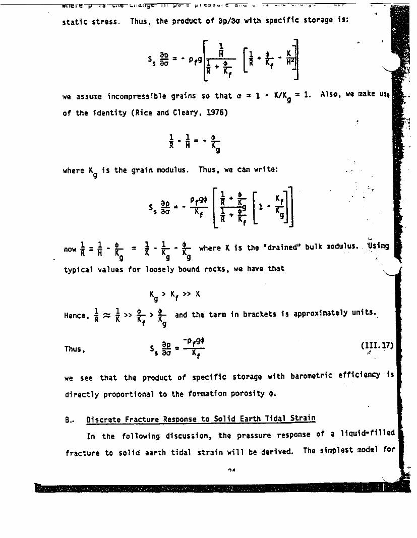
static stress. Thus, the product of ap/aa with specific storage is: IS5 a__Pfg W 4+ gi
we assume incompressible grains so that a = 1 - K/Kg 1. Also, we make Us0
of the identity (Rice and Cleary, 1976)
9
g~~~~~~~~where Kg is the grain modulus. Thus, we can write: .
typical values for loosely bound rocks, we have that
Kg > »f> K
Hence,~ » _ l > > L and the term in brackets is approximately units.
Thus, S a2 -fm (III. 17)
sao, Kf7
we See that the product of specific Storage with barometric efficiency is
directly proportional to the formation porosity O.
B.. Discrete Fracture Response to Solid Earth Tidal Strain
In the following discussion, the pressure response Of a liquid-flled
fracture to solid earth tidal Strain will be derived. The simplest model for
11..~ ~ ~ ~ ~ ~ ~~~~~~~I

W&k�-
Table 3.1
Frequencies of Major Tidal Constituents
- I
m.
Name (cycles/E) k
2Q. 0.0357063506 1
L C-0.0372185025 3
Ox 0.03873065 5
K ;s* 0.0417807462 12
JIL 0.0432928982 16
ZX2 s 0.0774870968 19
N2 0.0789992487 21
H2 0.0805114006 24
S2 b 0.0833333333 29
K2 0.0835614924 31
M3 0.1207671010 34
"I,}-
C�k
II
I I 'r, ,- =A. ~ - Mszet-

0w)= KAe "wk~~ 11.O.. .
I I UIL 2
where the finite set of frequencies (wk. k = 1,2, ...,N) are those shown
Table 3.1.
The tidal strain tensor near the surface of the earth takes; , Ie
the forM
i.(t) = 0ert eAA,( t ) heX(t)
he 3(t) -- e 9(t)
(III.22)
Therefore, equation (III.21) can be rewritten as:
K
P(w ) = - K [IO.wk[la wkie
A[ A(w0* 1 '88 (wk)l elk Cos2a2
Cos2C3
(Ill. 23)i-Ok
+ K I [te(Wk)I PI~A (W )I] e, �i;- A� -� -
O --
i la (wk)le K COS a2 Cos a3, k = 1,2, ... ,l
where the following relationships have been used to simplify the expression:
Verr = (eB + e)
Cos2 a1 + Cos 2 a 2 + CoS 2 3 = 1
arg (ee(wk)J = arg [eA(wk)J k
(see Major, et al., 1964)
and *d - arg Cex,(wk)] = t n/2- (111.24)
I J (see Major, et al., 1964)
-
26

t E It is useful to note that equation (III.23) reduces, for a vertical
r^ 5 Y fracture (a, = 90°) to:
|(wk)e k K leee(wk) Cos 2a3 + le.(wk)lCos2 az 4 i II (Wk)ICosa2
Cosa3 , k 1,2,...N (III.26)
25) and consequently, a vertical fracture with a N-S. strike (as 90°, a2 = 00)
- has the response:ar rr
a(wk)e k K le X(wk), k= 1,2 ...,N (111.27)
Gus and with an- E-W strike (as. a2 = 90°), has the response:
1ko(wk)e a K leOS(wk)I, k 1,2,...,N (111.28)
Thus, for a vertical fracture with either a N-W strike or an E-W strike, the)
measured fluid pressure responds in-phase with the tidal potential. Further-
o*re, based on equation (11.25), a fracture strike in the northwest quadrant
(Cosa2Cosa3>0) and a fractire strike in the northeast quadrant (Cosa2Cosa3WO)
xhibit equal phase shiftfiwith respect to the tidal potential, but of oppo-
)Site sign for a given tfe. Similarly, for the same strike quadrant, the
diurnal and semidiurnal tides also exhibit phase shifts with respect to the
iUl tidal potential of opposite sign.
I The fracture responseCmodel given above does not take into account fluid
leakage into the formation or the effect of a finite fracture permeability.
jio In the following discussioin', we develop a model of a discrete vertical bi-wing
ia s Or Penny-shaped fracture fi a permeable formation (see Figure 3.2). These
.Dll !" acture geometries approximate the actual geometries of a stimulated (hydrau-
e* -<-
.?

The (-/+) in equation (II.23) and Ft~h7--) in equation kiLi.ZT reer t
(diurnal/ semidiurnal) tides. If the measured pressure response at frequent,
Wk is now referenced to the tidal potential, and if a value of Poisson's4 rats,
is assumed, then:
P(wk)e k = K al(wk) + a2(wk) Cos2a2 + a3(wk) Cosa 3 + ia4(wk)
Cosa2Cosa3 , k 1,2,... ,N (111.25i
where the coefficients aJ(wk) and the phase of the tidal potential Ok art
known.
The possibility of computing a,, 02 and a3 (and hence fracture dip an .
strike) based on a single-well measurement of the pressure response at various
tidal frequencies is evident in equation (III.25). The solution of the set of
coupled equations given by equation (III.25) can be carried out with either of
two fundamentally different approaches. One approach is simply to solve t1i
set of N equations as a nonlinear least-squares problem to obtain not .onl
fracture orientation, but also the proportionality constant K. The latter v
yield useful information regarding fracture size and/or effective fractu X
storage given an appropriate elastic model for the fracture. The other _
approach, the one used in the analysis of the Raft River data (see Chapter
VI), is to recognize that although equation (II.25) includes both real and
imaginary parts, K is real. Therefore, the phase of the measured pressur,
signal, when referenced to the tidal potential, will be independent of .
Amplitude of the measured pressure response, however, depends strongly on K.
The dependence can be eliminated from the problem by evaluating equation
(III.25) for different frequencies wk. Since the fracture is assumed to have
large permeability, K will be Independent of frequency and therefore will
cancel when ratios of equation (III.25) are computed for different frequencies
28
__ __ _M M _06A

lically fractured) well. The motivation for choosing these geometries is
Q-i byprimarily for comparison with conventional pump test models that are currently
being used by the oil and gas industry for characterizing stimulated wells
(Cinco-Ley and Samaniego-V, 1981; Rosato, et al., 1982).
We begin by observing an element V of volume bounded by the surface
- within a fracture. The fracture opening has porosity * and the fluid filling
the open spaces of the fracture has density pf. The continuity equation can
. - be written (Ouguid and Lee, 1977) as:
p-f dV = 0 (Pfo) dV + |fPf¢<f>ds (III.29);-=. v v S
i;W-here A is the normal to the surface S and <Vf> is the space-averaged velocity
field of the fluid. The fluid velocity can be represented as the sun of the
Velocity of the solid<(V>plus the velocity of the fluid with respect to the
in ,J i! Solid, <Vf S>- or:
<Vf = (s> + <Vfs) (III.30)
OW including fluid velocity components along the fracture and normal to the
fracture (due to drainage to the formation), we may write, in accordance with
DaOrcy s law:
Of <Vt> = 8 f at 1 - ir ae (III.31)
Where I and 2 are the coordinates along the fracture and normal to the frac-
*>ture, respectively. kf' and kr are the permeabilities of the fracture and the
formations respectively. Assuming a slightly compressible fluid so that
Pf = (I [ Ps = po (1 + t ) (III.32)le

I
FORMATIONDAAINAGIS
T14
FORMATIOMDRAINAG3E
fi Figure 3.2. Finite vertical bi-wing fracture model and finite pennrshaped
fracture model. Formation drainage is normal to the fracture
plane.
m I i i
30

.1 -
N
I
where the fluid pressure p, with the exception of the integral term, is taken
to be an average value across the fracture. The integral in the last term in
equation (III.36) can be written as
-bfaf6!j dz = 2 z =bf2(III. 37)
where we have assumed a symmetric fluid pressure distribution about the mid-
plane of the fracture.
Assuming an oscillating normal stress of the form:
an(t) = an exp(iwt) (III.38)
It is easy to show that:
8o
z = b f/2r
(III.39)
where C. is the hydraulic diffusivity of the formation which is given by
krpfgCr =
5(III . 40)
Combining equations (III.36) through (III.39), we obtain:
V 22P - iwi bfC 2kr r-,II
bfkfc f kff Cr T bf C n(III. 41)
The above diffusion equation can be simplified considerably by redefining the
parameters into a dimensionless form:
kfbf
r(dimensionless fracture conductivity)
4"r,'. .i- - - . 1;� i - -
- - -10 ., 1z -- WV. . .
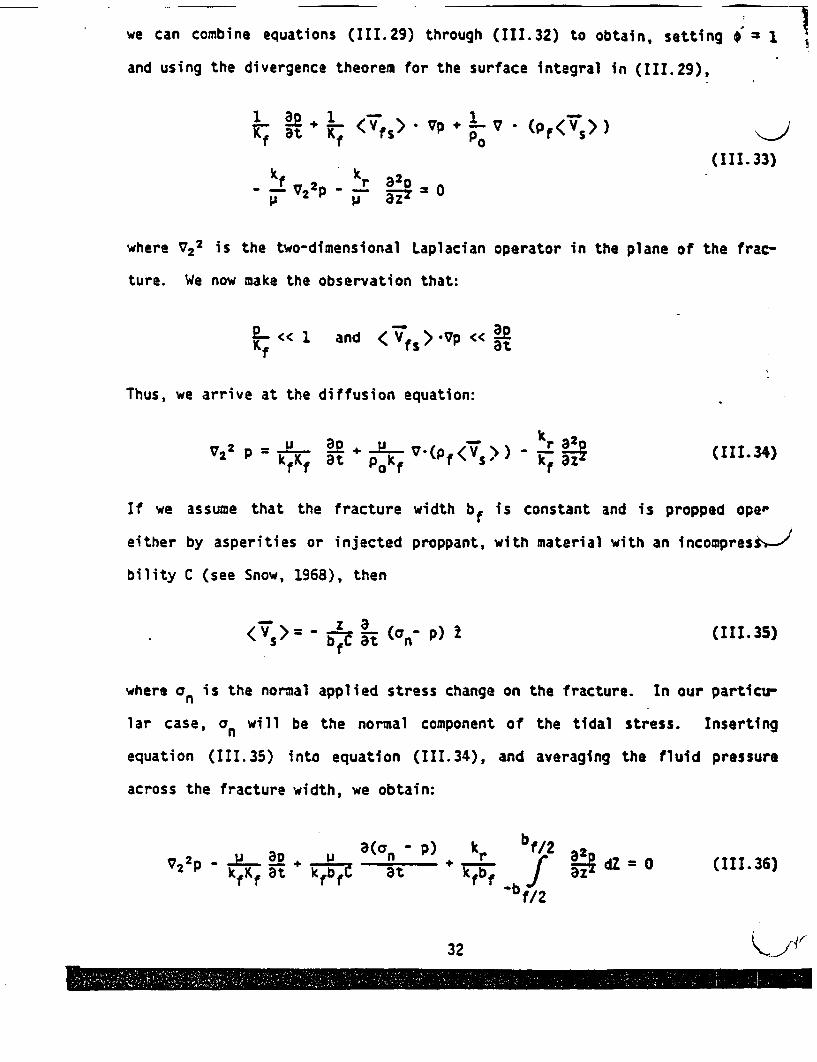
we can combine equations (III.29) through (III.32) to obtain, setting * 1
and using the divergence theorem for the surface integral in (III.29),
Kf at Kf < Vfs> PO V * Of<VS>
(III.33)k 2 P a2 o0
where V22 is the two-dimensional Laplacian operator in the plane of the frac-
ture. We now make the observation that:
P << 1 and < f>.VP <<a
Thus, we arrive at the diffusion equation:
2 p = - ap + p 1 .V(Pf(VS)) _ - - (III.34)72 ~ kfKf at pk f, kf HP(11.4
If we assume that the fracture width bf is constant and is propped open
either by asperities or injected proppant, with material with an incompresiv-'1
bility C (see Snow, 1968), then
< = q at xn rt ( (111.35)
where an is the normal applied stress change on the fracture. In our particu-
lar case, an will be the normal component of the tidal stress. Inserting
equation (III.35) into equation (III.34), and averaging the fluid pressure
across the fracture width, we obtain:
a~a -p) k b f/2 2V22p- _ U a + X n + .r | a2 dZ az (III.36)
kfK at kff~ at k fbf qa
32

" ." - - - -
and equation (15) reduces to:
V22 p a 41GI] = - iwd a (III.43')
The two dimensional Laplaclan takes the form
V22 = FE2 + 1 ar
for a penny-shaped fracture in which flow is purely radial, and
722 = 82
for linear flow. The conservation of mass boundary condition at the well-
fracture interface takes the form:
atp Ir-r= - aLpjrrw
(III.45)
Furthermore, we require a no-flow boundary condition at the crack tip, or:
iI8II = L
(III.46)
For the case of a vertical bi-wing fracture with height = H,
2gpfbf H
nrF2p Hf
2bf Kf-n 'pHII kfw15
, open-well with free liquid surface
shut-in well with positive' wellhead pressure
For the case of a penny-shaped fracture,
I � �-'e =� -11 r.

nf0 = Ct (dimensionless fracture diffusivity) (11132)
d = t-J (characteristic time)k
hr (porosity - total compressibilitywhere ACt C J product for formation)
and =OC 1 _1 (porosity - total compressibility(oCt~f Cbf Kf product for fracture)
We have adopted the porosity-total compressibility notation as opposed to the
specific storage notation to be consistent with the common well testing liter-
ature. L can be taken to be a characteristic fracture length, which is equal
to the half-length of a bi-wing fracture or radius for a penney-shaped frac-
ture.
With these definitions, equation (II1.41) can be rewritten as:
V2r1 2 [ 5 * - wd X -f ia (C11.43)VzP~Lzt7 f Ltzf jPL fD k fKf
The expression given by equation (II.43) can be simplified even further
noting that
[Lf~ f ] [ ] [1 + Cb ] (III.44)
Snow (1968) quotes a typical value for asperity incompressibility C of 4.33 x
108 Pa/m. Thus, assuming the fluid is water, the ratio Kf/(Cbf) yields a
value of 5.6x10² for bf as large as 1 cm. This ratio increases for smaller
fracture apertures. Therefore, we can to good approximation set the ratio
f f Lvr] - 3 [
34
I-I

pL~ -T A,-" w 1+7 ajLn a,,
(III.47')
where p. is the pore pressure response to tidal strain far from the fracture,
given by equation (III.16),
apfgPo = CrfAo
From equation (III.47'), we see that:
for a2 = 0
corresponding to
that
kf-
='r Ti~Prw ITP(III.48)
and
for a3 = 0
corresponding to(WIJCtkr)hL2
kfbf = 0kfb f
That PjIr--,_ T an (III.49)
In the first case (a2 = 0), the fracture. has no storage and the pressure
perturbation at the well is driven totally by formation pore deformation. In
the second case (a3 = 0), the formation has either no storage or no permeabil-
ity so that the pressure perturbation at the well is driven totally by frac-
ture deformation. Clearly, a realistic case will fall somewhere between these
two extreme cases, determined by the ratio
R =a 2 2fDat af,)
(wd)½h = 2 rOOt [I(Ct )fbf L w J (III.50)
* -= -7 - ,
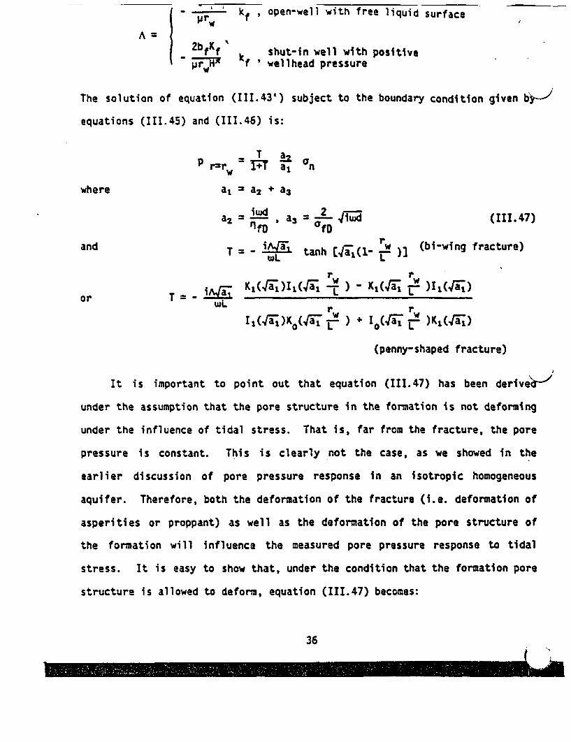
- |r' kf , open-well with free liquid surface
A=
Zbf f k shut-in well with positivePrv H f welihead pressure
The solution of equation (III.43') subject to the boundary condition given b -
equations (III.45) and (III.46) is:
.T 1Zc7
P r__rW i7 al n
where a, = a2 + a3
a 2 = . a3 5 .L vji (III.47)
and w tanh t rw ) (bi-wing fracture)
r ril K1(4a_1)I1,(4al, wL ) - KI(4a r-L )11( ^a )
or T - _LL K(4 )1( )wL r r
I1(4iaj)KO(4a' Lw ) + I0(Gi r- )K 1(4I)
(penny-shaped fracture)
It is important to point out that equation (III.47) has been derive,-
under the assumption that the pore structure in the formation is not deforming
under the influence of tidal stress. That is, far from the fracture, the pore
pressure is constant. This is clearly not the case, as we showed in the
earlier discussion of pore pressure response in an isotropic homogeneous
aquifer. Therefore, both the deformation of the fracture (i.e. deformation of
asperities or proppant) as well as the deformation of the pore structure of
the formation will influence the measured pore pressure response to tidal
stress. It is easy to show that, under the condition that the formation pore
structure is allowed to deform, equation (III.47) becomes:
36

I
where nia is the normal component of the strain tensor. Therefore, equation
(III.47') can be rewritten as:
T
=~r FT t,, ( ) ( ) +a p6] (111.51)Plr-rw 1+Tat a, a,
The first term in the brackets is the response due to shear deformation of the
fracture. The second term is the response due to a volumetric (isotropic)
strain of the fracture. The last term in the brackets is the response due to
pore deformation in the formation. The multiplier T/(1+T) can be considered a
tidal "transfer function" between the fluid pressure in the fracture and the
measured fluid pressure in the well.
For a vertical bi-wing fracture whose spatial orientation depends only on
strike, it is clear from equations (III.47') and (III.51) that in the most
general case, the measured pressure response depends on four hydraulic param-
eters and one orientation parameter. The hydraulic parameters are: a2, a3,
Ss/a, and A/L. For the case of a penny-shaped fracture in which dip is not
constrained, the total number of free parameters is six. We have assumed that
X and p are known and that the strain tensor can be estimated (see Chapter
II). The number of free parameters is reduced for the case in which the
formation permeability kr = 0. In this case, a3 = 0 and al = a2. For a
vertical fracture, there are three free parameters and for an unconstrained
orientation case, there are four free parameters. Since under most practical
situations we usually have amplitude and phase information at the two tidal
frequencies corresponding to the 01 and M2 tides, we have a total of four
equations. Therefore, the solution will be unique only under the situation in
which there is little or no drainage to the formation. If there is drainage,
the solution will be under-determined. Recovery from the latter situation can
..... -

* .-. nr .:-y to tracture Cefor-
mation. If R>>1, the pore pressure response will be due primarily to drainage
effects caused by pore structure deformation in the formation. In order to
get a feeling for the dependence of R on the host rock permeability, we h-
evaluated equation (III.50) under the assumption that the pore fluid is wat ir,
Oct = 1.5x1O-10 Pa and that the asperity incompressibility is 4.33xlO8 pa/m.
With these assumptions,
R = 0.9 4kr(md)
Hence, we see that if the formation permeability is on the order of 1 ad, the
pore pressure response to tidal stress is divided roughly equally between
fracture deformation and formation pore structure deformation. With the
exception of the case in which the formation has a permeability in the micro-
darcy range (e.g. crystalline granite), it is clear frbm the above exercise
that equation (III.47') must be used as the appropriate general tidal response
model.
Hooke's law for isotropic elastic bodies, written in tensor form, i\>
aik :- aik +2eik
where A and W are Lame's parameters, defined in terms of Young's modulus E and
Poisson's ratio v, as
X~~~=(1+)(1-2V)
Thus, the normal stress an in equation (11I.47') can be written as:
an= AA + 21J AZA 3
38
L -

I _ gi -4 _'.L.t -- - - _'V - -4X ' I.S .,- ... - .- - -. __ - I i " -.WI _1
CHAPTER IV
INTEGRATION OF TIOAL RESPONSE WITH CONVENTIONAL
PUMP TESTS FOR FRACTURE CHARACTERIZATION
The previous chapter indicates that, under some conditions, additional
information will be required to calculate a unique fracture orientation solu-
tion. A conventional well pump test will, in principal, yield the needed
information. Indeed, with proper test design, it will be possible to obtain
the tidal pressure response information simultaneously with a conventional
well pump test.
Another possible method for determining system hydraulic parameters from
a pressure transient test is that of multi-frequency flow testing (Hanson,
1983). This method is a variation of conventional testing methods that may
allow for better parameter resolution and can also be carried out simultane-
ously with tidal response monitoring.
As an example of the integration of tidal response with a conventional
pump test, we consider a build-up test on a stimulated well with a vertical
fracture (Cinco-Ley and Samaniego-V, 1981). A well is flowed for a time t1 at
a constant volume flow rate q and is then shut-in. The diffusion equation
appropriate to this situation is (see Equation III.36):
V22p- ~~Kf kr bf/2 2I.1V2p - 1+ f 80 + r '/2 0 (Y
Rather than assuming an oscillating solution, as we did in equation III.38, we
Laplace transform equation (IV.1) to obtain
V22 p -- S C(1 + rf ) (p -_ - ) - k s (p - ) 0 (IV.2)bff f f f r
be accomplished if some of the hydraulic parameters are known a priori' or if
information at other tidal frequencies is available. The next chapter shows
how this information can be obtained using a conventional pump test if pres-
sure response data at other tidal frequencies is not available.
40
��I

A1 - a2 + a3
a = ds a3 = ds
H is the height of the fracture at the wellface.
The pressure history from the beginning of flow at t=O to time of shut-in
tot1 and later can be obtained by calculating the inverse Laplace transform of
equation (IV.6). An analytic expression for the inverse is likely to be
difficult to obtain. Therefore, a numerical approach (Stehfest, 1969) is the
most expedient. Since there is a discontinuity in 8p/Ot at t-tl, a direct
numerical inverse will not obtain a reasonable precision near tzt1 . We there-
fore modify the numerical inverse procedure to take advantage of the time
translation operator associated with the term exp(-tls). Calling
G(s) = AL 1
s 4ia tanhtil(l - rw/L)J
it is easy to show that
P(t) - p(t=O) = t(1-e t1s)G(s)]
r - _, (IV.7)= x[G(s)]t - C G(s)]t_ tlU(t-tj)
where U is the Heaviside step function defined by
O. tstjU(t-t1 ) =
U~t~t0 1, Vtlt
and the subscripts t and t-t1 indicate the time at which the Laplace inverse
is to be evaluated. By this procedure, the function G(s) which is to be
inverted numerically, is well-behaved.
--- ;.� -W. .III
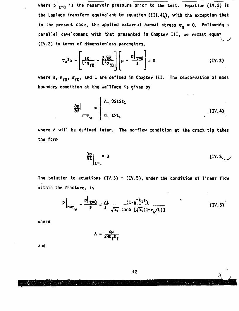
where pjo is the reservoir pressure prior to the test. Equation (IV.Z) is
the Laplace transform equivalent to equation (III.4A), with the exception that
in the present case, the applied external normal stress an = 0* Fcallowifg a
parallel development with that presented in Chapter III, we recast equat
(IV.2) in terms of dimensionless parameters.
v2 p s[ ] 0 ] (IV.3)
where d, nfo. af,) and L are defined in Chapter III. The conservation of mass
boundary condition at the wellface is given by
A, 0Ststl
at | = (IY.4)r--r. O. tatj
where A will be defined later. The no-flow condition at the crack tip takes
the form
=0
The solution to equations (IV.3) - (IV.5), under the condition of linear flow
within the fracture, is
irr sI AL (__ e-_ts)___6)
w S S tanh [ (-rL)](IV.6)
where
A=*MaHbfkf
and
42
0

We have used the time derivative of pressure to determine the constraints in
order to eliminate the requirement of knowing the initial static reservoir
pressure. If this information is known, the above conditions of constraint
are easily modified.
Equations (IV.8a,b) represent the situation in which linear formation
flow regime has been achieved (see Cinco-Ley and Samaniego-V, 1981). This
condition is exhibited under the condition of high fracture conductivity,
afDo300. The pressure within the fracture equilibrates rapidly and subsequent
pressure changes are due to drainage from the formation. Equation (IV.8c)
represents the bilinear flow regime in which a linear flow occurs simultane-
ously in both the formation and the fracture. A detailed description of the
conditions under which bilinear flow can be expected is given by Cinco-Ley and
Samaniego-V (1981).
As an example, we consider a vertical fracture of half-length L = 100 m,
width by bf = 1 mm, and height H = 50 a. The asperity incompressibility C =
4x10⁸ pa/m and the formation fluid is water. The formation has a permeability
kr = 10 md and a porosity-total compressibility product OCt = 7.3x10⁻¹" pa-l.
The well is flowed for 24 hours at a volume rate of 10 M3/hr and is then
shut-in. Under these conditions, af0 = 83.3, '1f= 241.5,-d = 20.1 hr. and AL
4.8 psi. Thus, the three model parameters are:
Of 9.29 hr 124d
11f= 12.02 hr-'
AL - -4.8 psi
Figure 4.1a shows the pressure history and Figure 4.1b shows the time deriv-
ative of the pressure history based on the numerical Laplace transform inver-
# _ .IS Do,_, _ ~--Za

A least-squares fit to equation ('V.7) to obtain the three system param-
eters AL, nfD /d, and afo/(24d) will require a considerable computational
effort unless some a priori information is known about the reservoir. However,
under certain conditions, the number of free parameters in the model cLa_,
reduced from three to two. Under these conditions, it is a straightforward
procedure to calculate the mean squared error, or chi-square, as a function of
the remaining two parameters for a reasonable range of parameter values. An
approximate value of the two unknown parameters can be obtained from the
minimum of the chi-square function. These estimates can serve as an initial,
or starting, value for a more refined inversion scheme such as a Marquardt-
type scheme or a grid search. The constraints that decrease the number of
model parameters from three to two are generated using the following-relation-
ships
X lim Cs F(s)] = lim f(t)-s54 t+O
.1Z lim Es F(s)] = lim f(t),
s*O t-OM
it is easy to show from equation (IY.6) that
(l) lim do =~FLf~- l~t" dt 2rd 4 J
or lim = (i do/dt (AL) - (IV.8a)t"m 1/4 - 1/4Tt_-ti) V~t 2t
l> { d } =) (AL) '' (IV.8b)t-" d~tt 24?
(2) lim do A [A{l f]
or ulr { (4t) 3/ 4 do = ALj~!2D (IV.8c)
44 K>

the asymptotic value of (AL)(of0/4d) = 1.41 has not been reached after 300
hours into the test. Because of the large fracture length, there is probably
still a component of the bilinear flow regime contaminating this information.
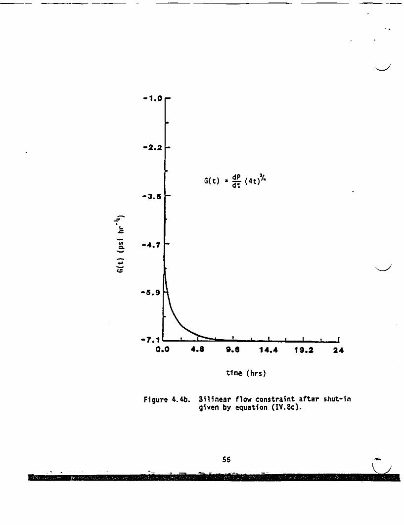
Bilinear flow is clearly indicated by Figure 4.4b which is a plot of the
constraint given by equation (IV.8c). The discrepancy between the theoretical
asymptotic value
(AL)( -D ) = -8.23 psi-hr~24d
and that shown in the figure, namely -7.1 psi-hr A, is likely due to the
approximation inherent in a numerical Laplace transform inversion.
The fact that the bilinear flow dominates prior to shut-in is substanti-
ated by Figure 4.4c which shows a plot of the constraint given by equation
(IV.8b). The theoretical asymptotic value, which is not reached prior to
shut-in, is
(AL)( f) = -1.41 psi/4hr24d
The examples presented above are primarily for illustrating the fact that
the flow parameters for a fractured reservoir can in principle be obtained
given some realistic model for the reservoir. We have chosen a vertical
bi-wing fracture model to be consistent with the tidal strain response model
given in Chapter III. It is not surprising, therefore, that the model pre-
sented here shares the same hydraulic parameters as the tidal response model.
Given an evaluation of these parameters by a conventional pump test, the
non-uniqueness of the fracture orientation model given by equation (III.47)
can be overcome.
iI
-� .-.,

sion of equation (IV.6). Figure 4.2a shows the evaluation of the constraint
given by equation (IV.8a) for the limit of linear formation flow. From this
figure, it is clear that the plotted function is approaching asymptotically a
value roughly -44.5 psi/4hr. The actual value is given by:
(AL)( ) = (-4.8psi)(9.29hrh) = -44.6 psi/4hr24d
Figure 4.2b is a plot of the constraint given by equation (IV.Bc). From this
figure, we conclude that, at least prior to shut-in, the bi-linear flow regime
is not obtained. This observation is substantiated by Figure 4.2c, which is a
plot of the constraint given by equation (IV.8b). It is clear that, prior to
shut-in, the fracture conductivity is large enough for the flow regime to
approach a linear formation flow. This figure shows that the constraint given
by equation (IV.8b) asymptotically approaches -44.1 psi/4hr where again the
actual value is -44.6 psi/4hr.
A second example is presented which is identical to the example given
above with the exception that the fracture half-length L is increased from',.
m to 1000 m. With this modification, afD = 8.33, nfo = 241.5, d = 2.01x10⁴
hrs, and AL = -48 psi. Thus, the three model parameters are
fo = 2.938x1O-2 hr1h24d
d = 1. 2x10⁻² hr-1
AL = -48 psi
Figure 4.3a shows the pressure history and Figure 4.3b the time derivative of
the pressure history under these conditions. Again, we have plotted the
equations of constraint given by equations (IY.8a,b,c). Figure 4.4a shows the
linear formation flow constrain given by equation (IY.8a). It is clear that
46)
- �1�_

L
-3
-231-23
S.-
C.b0-
1 SHUT-IN
0 60 120 *80 240 300
time (hrs)
Figure 4.1b. Time derivative of data shown in Figure 4.1a.
4 -..--.
AO

-88
SHUT-IN
-130.
c.
-170
"-2120 s0 120 780 240 300
' time (hrs)
Figure 4.1a. Pressure history during a drawdown-buildup pressure transienttest. Well is shut-in at t = 24 hours and L = 100 n.
48 K

I
- 4
G(t) a 1 (4t) .
It
I-
C:
-95
-125 -
0.0 4.8 9.6 14.4 19.2 24.0
time (hrs)
A Figure 4.2b. Bilinear flow constraint after shut-in
given by equation (IY.8c).
51 .- - . ... W .

-40.5
-41.6
-42.3
-43.0
G v)- i dP/dt 1
S.
4.9
- 4 4 .35 I --- I 9 I I V
30 84 138 192 246 300
time (hrs)
Figure 4.2a. Linear formation flow constraint given in equation (IY.8a).
50

i'
-0.6
-3.8
-7.0
-10.3
-13.5
U'
Z7C.
0 60 120 180 240 300
time (hrs)
I Figure 4.3a. Pressure history during a drawdown-buildup pressure transienttest.. Well is shut-in at t = 24 hours and L = 1000 m.
4I

J
15
(a
-7.3
-15.1
-22.3
-29.6
-38.8
-44.1 _0.0
G(t) . dZ OFFdt
4.8 9.0 14.4 19.2 24.0
time (hrs)
Figure 4.2c. Bi i neargiven by
flow constraint before shut-inequation (IV.8b).
52 I
M

;
-1.6
-1.9'
-2.3
4.1
G(t) = dt
GT - t7
-2.7
-3.1
- 3 .5 v130 84 138 192 246 300
time (hrs)
Figure 4.4a. Linear-formation flow constraint given in equation (IV.8a).
.1p

2.4
-0.9
L.
s~ -2.6 -
-W
-4.2 -
W5.91 I, - I I I 1 I I I I I
0 00 120 180 240 300
time (hrs)
Figure 4.3b. Time derivative of data shown in Figure 4.3a.
54
Al1

-, ---
R91-i"
-2.0
-2.7
-3.5
ft.�
7;OL
.W
Q
G( t) - ddP A
-4.2
-5.0
-5.70.0 4.8 9.6 14.4 19.2 24.0
time (hrs)
Figure 4.4c. Bilinear flow constraint before shut-ingiven by equation (IV.8b).
-1.0
'-
L.
-2.2
-3.3 -
-4.7
-5.9
-7.10.0
G(t) - dP (4t)%dt
4.8 9.6 14.4 19.2 24
time (hrs)
Figure 4.4b. Bilinear flow constraint after shut-ingiven by equation (IV.8c).
56-11
.
K I

CHAPTER V
SPECTRAL ANALYSIS, CORRELATION, AND ERROR ESTIMATION
Extraction of information from signals of tidal origin requires the use
of Fourier spectral analysis methods. However, due to the fact that the tidal
spectrum is a line spectrum with all energy contained within a finite Dirac
delta distribution (ignoring the small non-linearity introduced by the ocean
tide loading effects), certain modifications of conventional spectral analysis
methods are required. These modifications make use of the fact that the tidal
frequencies are known with great precision which consequently reduces the
number of degrees of freedom of the problem and therefore improves the tidal
amplitude and phase estimates. This improvement of tidal signal resolution
was first discussed by Munk and Hasselman (1964) for the simple case of two
neighboring spectral lines. An extension of this approach to the full tidal
spectrum is discussed in some detail by Godin (1972). One can show that this-
approach can improve signal resolution over the classical Rayleigh resolution
criterion. The latter states that, for a signal record length L, two spectral
lines separated in frequency by &f can be resolved if LAfMM/2.
In the following, we will present a discussion of line spectral analysis,
beginning with the idealized case of a continuous signal of finite duration
followed by the case of a discretely sampled signal of finite duration.
Assuming that, in the practical case, some amount of noise will be present in
the signal, a formulation of the varlance-covariance matrix and the subsequent
translation to uncertainty in the amplitude and phase for each tidal constitu-
ent will be presented.
We will first begin with the ideal case of a noiseless continuous tidal
signal f(t) on the time interval -L/2 1 t 5 L2 consisting of N discrete fre-
-. - a. -. _ _ An_-I_
I
I
d
r. a

quencies [wl, w2, ... , w.) with amplitude and phase distribution Jal,41;
a 2 ,0 2 ; ... ; aNON). The signal can be represented by the sum:
Nf(t) = I anCos (wnt + °n)
n=1
The finite Fourier transform of f(t) evaluated at frequency wk is given by:
_L/F(w ) = 2 ) eiWkt f(t) dt (Y.2)
k t- 2
which, upon insertion of equation (V.1), obtains the following expression:
N . Sin( + W L) Z I Sin[(w - w ) U2]
F(wk) 2 L a eln Iun * Wn) (wk - Wn) J (V.3)
If we now define:
n = a ein (V.4)
Z= RZ1, Z2, *- ZN)T (
F = {F(w1), F(T2), T (V.6)
± SSin[(wk ± wn) U/2(Akn (wk ± w ) L/2 (Y-7)
Equation (V.3) can be recast as a set of N equations and N unknowns, given by
the matrix equation:
A+ + A =F (V.8)
where the elements of A and A are given by equation (Y.7) and ZF is the com-
plex conjugate of Z. The unknowns, namely amplitude and phase the tidal
constituents, are contained in the complex vector Z.
60
a

O", �HMMMWMMIBM
Separating the real and imaginary parts of equation (V.8),
Re r= (A+ + A-) Re T
ImB= (A+ - A-) In )
The complex vector T = Re T + iIm T can be written as:
Z Ho Re T + i H Im T (V. 10)
where H (A++ A-)- 1- 4 -A-1 (V.11)
H = (A - A )
Equation (V.10) gives the vector of N unknown complex tidal constituents
in terms N complex finite Fourier transforms and two real symmetric matrices
H and H that serve to couple F with Z. The finite Fourier transforms can
easily be estimated using numerical integration methods. It is important to
point out that the coupling coefficients depend on the duration L of the
signal and the location of the frequencies in the tidal spectrum, as indicated
by equation (V.7). It is also noted that, as the duration of the signal L
gets large, that
A+n 0 ° and Akn 6kn
and thus
H I and H + -I
where 6kn is the Kronecker delta and I is the unity matrix. In this limit,
T.I +T (V.12)
and the complex tidal constituents become uncoupled from each other. It is
clear from the above that, if a conventional Fourier analysis of a finite
length of data is carried out for the purpose of extracting the tidal constit-
t 61

uents (see equation (V.2)), an error in the estimates will be found due simply
to the finite length of data independent of any noise that may also exist on
the record. This is discussed in some detail by Blair (1979). Therefore,
equation (Y.10) should be used over equation (V.12) for the purpose of
tracting tidal information from a record.
If the tidal signal is a discretely sampled function and not a continuous
function, the form of equation (V.10) is maintained although the expression
for the matrix elements AOkn given by equation (V.7) is modified to take into
account the discrete sampling. The derivation of this expression is similar
to that presented for the continuous case although the algebra is somewhat
more involved. Therefore, the results will simply be stated:
M2At I inatw (.1F(wk) =r rEM f(nat)e k (V.2')
A - Sin((Wk V w)) L/23 V.7'k; ~~r Snl(wk :t at t/3(
where L=(2M-1)&t and the solution vector 2is obtained by equations (V.10)
(V.11). It is evident from equation (V.7') that as at.0, the expression for
Atkn approaches that for the continuous case, namely equation (V.7).
The variance-covariance matrix, which contains the necessary information
to estimate the uncertainties in the computed amplitude and phase of the tidal
constituents, can be formulated relatively easily. The formulation presented
here assumes that the noise, n(t), is "white" -- that is, the amplitude of its
ensemble average is uniformly distributed with respect to frequency. If the
noise is random, it is automatically "white" noise (Goldman, 1968). We assume
that the noise-contaminated signal is given by:
g(t) = f(t) + n(t) (V.13)
62
0

--- � I - -
where f(t) is given by equation (V.1). Assuming again for the purpose of
illustration a continuous signal, as opposed to a discretely sampled signal,
we may define:
L2
G = A ZI + A Z*, + [eiWkt 4(t) d (V.14)
where we have simply replaced f(t) with g(t) in equation (V.2). The last term
in brackets is a column vector whose elements range from k = 1 to k = N. Z is
again the true spectrum (no noise) of the tidal record. If rF is defined as
the measured value of the spectral constituents, then we can also write:
A+ r + A- r (V.15)
Defining an error vector between the true values and the estimated values of
the spectral constituents as:
ir = 7 - 2
we can use equations (V.14) and (V.15) to derive the following expressions:
2+ - r~~~U 2wtRe 2r (A + A 1Cos (W t) h(t) dtI ccl
(V.16)L2
Im 'r= 2 (A.- A-)1 [Sin (wkt) F(t) dt]co
where the terms in brackets are column vectors whose elements range from k=1
to k=N. The ensemble averages of the following expressions are now obtained:
(a) <(Re Zr) (Re &r)k>
(b) <(Iu rr)j (Im rr)k' (V.17)(c) <(Re r)j (I. r)k >
63

with the assumptions that the noise is a stationary time series and ts also
"white", then the ensemble average of r(t)n(t') is given by:
<q(t) n(t')>= 2n SO(w) 6(t-t')
where S (w) is the noise power spectrum. If we assume that the signals are
band-limited such that no energy exists beyond the Nyquist band, then
So(w) = a2 r (V.18)
where v2 is the mean-squared error of the signal and at is the sampling rate.
With the same algebra, it can be shown that the ensemble averages of equations
(V.17) are given by:
<(Re P) (Re ,7) =2L H Jsk = 1,Ni O ~~L jk
<(Ix Pr). (I 3r)k= -c-t jk Jk = 1,N (V.19)
<(Re Xr) (Im rr)k>= , j,k = 1,N
where H is given by equation (V.11). For a discretely sampled signal, the
definition for At given by equation (V.7') is used. v2 can be estimated by:
L/2v2 = [g(t) - f(t)]2 dt (V.20)
-/2
where f(t) is the least-squares approximation of f(t) using the computed tidal
constituents F. It is easily shown that 7 is the best estimate of 2 in the
least-squares sense.
Expressions given by equation (V.19) represent the variance-covariance in
the real and imaginary components of the N spectral estimates. It is impor-
tant to point out that, based on these equations, the uncertainty of the
64

; spectral estimates can be reduced either by increasing the sampling rate (i.e.
decreasing at) or increasing the duration L of the record length. Therefore,
at least in principle, signals of tidal origin, or any stationary repetitive
signal for that matter, can be resolved regardless of the background noise if
the sampling rate is sufficiently fast or the record length is made suffi-
ciently long.
Probabilities can be assigned to the uncertainties in the spectral esti-
mates if a form for the probability density function is assumed. We have
assumed a two-dimensional normal distribution where the two random variables,
namely (Re rr). and (Im Er)j, are uncorrelated. The latter is reflected in
equation (V.19) where the ensemble average of the product of these two vari-
ables is found to be zero.
The probability of finding a point (X,Y) in the ellipse defined by the
equation:
_x ] [- z 3 2 k2 (V.21)
is equal to 1-e k For the case under consideration, (pxt Py) are the expec-
tations of the real and imaginary parts of a given tidal constituent and (a 2
: g ay2) are the variances of these estimates, respectively. Therefore, at a
confidence level 4, ranging from 0 to 1, the axes of the error ellipse in the
complex plane have half-lengths of:
a = 4-2 ln(- a)' aX
b = 4-2 ln(- a)' y
where a 2 t + 1aX =1-HiX LL i
11- _'T__ - PC r , - -'L_� jg!2=gp� M-figm- Qkw_ �.: 1.. - MWV5_�

for the jth ti1al constituent. Figure 5.1 serves to illustrate this. Uncer-
tainties in amplitude and phase of the jth tidal constituent at the confidence
level t can easily be obtained by numerically mapping the above error el a__,
from the complex domain (real, imaginary axes) to the amplitude-phase domain.
In the practical case, the measured pressure record will include effects
due to barometric loading and well pumping. These effects must be removed
from the measured pressure record prior to carrying out the spectral analysis
procedure discussed above. A somewhat involved, but straightforward procedure,
is used to accomplish this. Figure 5.2 shows a data analysis flow chart from
data measurement through data interpretation. We begin by assuming that the
measured fluid pressure data can be represented by:
p(t) = f(t) + fb(t) + f p(t) + F(t) (V.22)
where f, fb' fp, and q are the tidal, barometric, pumping, and random noise
constituents, respectively. In general, fb and f will have fluctuations wr!"h
longer periods and larger amplitudes than f. We therefore fit a trend fure'
tion, using either spline and/or least-squares polynomial fitting, to p(t) to
obtain a first approximation to the sum fb(t) + f p(t). This trend function is
then subtracted from p(t) to obtain a first estimate of f(t) + n(t). Using
this first estimate of the tidal component, we carry out a tidal line spectral
analysis as discussed previously to obtain a first estimate of the amplitudes
and phases of the tidal constituents. This signal in turn is subtracted from
the measured fluid pressure data to obtain a second estimate q(t) of the sum
of the pumping and barometric effects. The barometric loading effect at the
tidal frequencies will of course be minimized in this signal. In a similar
66

Im p V-2 a -- I
2b
IRe P
a
49
Figure 5.1. Example of uncertainty error ellipse of a tidal constituent inthe complex plane.
- .. ;i .. .s

TIDAL ANALYSIS METHODOLOGY
BAROMOITRIC PROSUR& TWIOS FROM R~tDt
CALCULATI UNE SPECTRALTHIORETICAL ANALYSIS
GRAVITY A STRAIN
ASMPLITUDES/PHASESUNI SPECTRAL OP TtOAL PrEouINc1s3
ANALYSIS IN WELL PRESSURE DATA
AMPLITUDES/PHASES |A ICIENCT
CaRAVTY A STRAIN
MODEL
Figure 5.2. Flow chart showing the various stages of tidal data processingand analysis.
68
I -- L,

-
- -
3
I
fashion, we also remove from the measured barometric pressure pb(t) signals at
the tidal frequencies. The resulting signal r(t) will be used, in conjunction
with q(t) to obtain estimates of the pumping and barometric effects. This is
carried out by minimizing the following integral:
I = y tq(t) - BE-r(t) - SN(t)J2 dt (V.23)
with respect to the barometric efficiency, BE. SN is an N-knot spline. The
minimization is carried out by choosing a value of BE, evaluating q(t) -
BE-r(t), fitting an N-knot spline to this function, and evaluating the mean
squared error between q(t) - BE-r(t) and SN over the recording period [ti,
t2 J. The process is repeated for various values of BE until I is a minimum.
The result yields: 1) an estimate of the barometric efficiency BE, and 2) an
estimate SN of the pumping component. It is emphasized that we have assumed
that the permeability of the reservoir is sufficiently high so that there will
be no time lag between the applied barometric load and the fluid pressure
response. Criteria for this assumption are given in Chapter III. An uncer-
tainty in the barometric efficiency BE can be estimated by fitting a straight
line to the parametric equation
y(t) = q(t) - SN (t)
x(t) = r(t)
and calculating an uncertainty in the slope BE.
Finally, the pressure signal constituent associated with the tidal re-
sponse is obtained according to:
f(t) + n(t) = p(t) - BE pb(t) - SN(t)i
� - --% - : - --�15�-V *� - .

-7
OL
1rN

CHAPTER VI
CASE STUDY - RAFT RIVER GEOTHERMAL AREA
The Raft River geothermal field is a low temperature, single-phase
(liquid) system located in southern Idaho near the boundary between the Snake
River plain and the Basin and Range province (Figure 6.1). It is situated
within a north-trending upper Cenozoic structural basin filled with nearly
1,600 m of tephra and sediments derived from the surrounding mountains.
North of the Raft River basin is the Great Rift system exhibiting open
fractures in young basalt flows that extend northward 50 km to Craters of the
Moon National Monument. The basin is flanked to the west and south by the
Albion and Raft River mountains which expose gneiss-dome complexes of Precas-
brian adamellite mantled by Precambrian and lower Palezoic metasedimentary
rocks (Felix, 1956; Armstrong, 1968; Compton, 1972). Drill hole data have
demonstrated that a Precambrian and lower Paleozoic metasedimentary complex
directly underlies the Cenozoic fill of the Raft River basin (Dolenc, et al.,
1981). The two principal faults exposed within the valley are two north-
trending normal fault zones along the west side of the valley called the
Bridge and Horsewell fault zones. There is also some geologic and geophysical
evidence (Mabey, et al., 1978) suggesting a possible basement shear, called
the Narrows Structure, that trends northeast across the valley. It has been
noted (Covington, 1980) that the abundance of faults and fractures increases
with depth. In the upper part of the basin fill the faults dip steeply (60°-
80') and with increasing depth, fault dip decreases until they become nearly
parallel with the contact between the fill and the Precambrian basement.
Movement along these normal faults produce abundant, and near-vertical, open
fractures near the base of the basin fill (Covington, 1980; Guth, et al.,

1981). A structure cross-section along line of section B-B' in Figure 6.1 4i
shown in Figure 6.2. A
In 1971, the United States Geological Survey declared the Raft Rive-
valley a Known Geothermal Resource Area (KGRA). Since 1974, seven deep wei
ranging from 1176 m to 1994 a, have been drilled (Figure 6.3). Four produc-
tion wells, RRGE-1,2,4, and 5 were drilled near the intersection of the Bridge
Fault and the Narrows Structure. Another production well, RRGE-3, was drilled
away from the major fault zones to see if the resource extended into the
valley. All of the production wells were drilled into the Precambrian base-
ment. Two intermediate-depth wells, RRGI-6 and 7, were drilled further east
for the purpose of reinjecting spent geothermal fluid. These wells are com-
pleted in the Salt Lake formation, a tuffaceous sandstone, siltstone, conglom-
erate sequence. Figure 6.4 shows the distribution of depths and the forma-
tions penetrated by the wells. No significant wellbore skin damage has been
observed at the Raft River wells. From 1974 to 1982, extensive geological,
geophysical and hydrological testing and analyses were carried out at Raw
River under the auspices of the U.S. Department of Energy (Dolenc, et al 1
1981). The Raft River reservoir was an ideal location to test the solid earth
tide response methods because of the vast amount of conventional reservoir
evalution work carried out during the past decade.
Conventional well pumping test data taken between 1975 and 1979 were used
for the tidal response analysis. Pump test duration ranged from 6 to 37 days
with pressure measurement sampling rates of every half hour or every hour.
Wellhead data were obtained during the tests with Paroscientific pressure
transducers. The raw data are shown in Figures 6.5-6.11. Downhole data were
taken with a Hewlett-Packard temperature-compensated quartz pressure probe.
The tidal fluctuations are clearly evident on these data. The pressure record
72

4
In!6
Z
Figure 6.1. Raft River Valley and major structural features adjoining thevalley (from Dolenc, et al., 1981).
r
i
NOMMEwiv- - ~~~- *~~~~U0t

F I
Tertt"rRhyaUte
B.
2000
150I-a10000&d
30 0 " .. 8 r -- ~ - - . .
40 1.*-.. .a
Preca mnbrian A da e it % . u ec o .
(Covington, 1980)
Figure 6.2. Cross-section 8-83 of Figure 6.1 (from Covington, 1980"
74
I

Figure 6.3. Geothermal well locations within the Raft River Geothermal Field.
X.= -2 f L - -
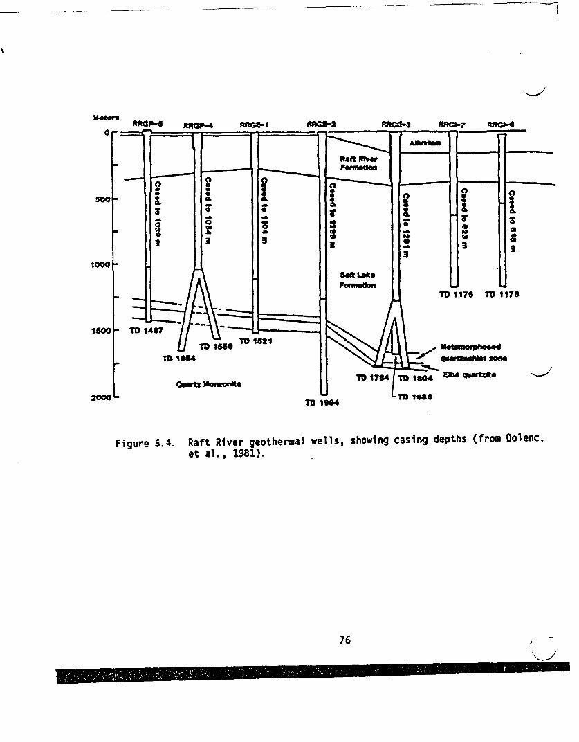
"on~r
ori
I500
1000
1500
2MM a tT It"
Figure 6.4. Raft River geothermal wells, showing casing depths (from Dolenc,et al., 1981).
76
M- ~ ~ ~ ~ ~ ~ -

li
57 0%.M U I
RRGE -1
C,,
'U-J.0zo0o
0
572.01-
l671.0 I ..1.I .. I. .. .
60 100
TIME (HRS)
150 200
Figure 6.5. Raw downhole pressure data at RRGE-1.
I
.I - 0. -Shm, " A' 0 en & � -I-. .

Imc-
af'
w-
w
v)
co
zLU0
0
200 400 Goo 80
TIME(HRS)
Figure 6.6. Raw downhole pressure data at RRGE-2.
78 II

115.1
LU
C,,
CL
.j1LU
114.71
114.5
114.25
a 100 200TIME (HRS)
Figure 6.7. Raw welihead pressure data at RRGE-3.
K><.~~~~~~~~~~~ .~~~~~~~~~~ ~ ~ ~ ~

139.Jj .
RRGE-4
Im
CD,
0..0wi-J-JCO
138.0
137.0
1A f I I I I I I I
s0 100
TIME (HRS)
150
Figure 6.8. Raw welihead pressure data at RRGE-4 showing pulse test.
80j
-~~~~~~~~~~~~~~~~~~~~~~~~~~~~~M~ ~~~~~~~

S%
RRGI-6
1-%
Cl5 24.0CL
LU
LU
-j-JLU
C:
I-_
23.51-
. .. . I I I. . .0 100 200 300
TIME(HRS)
Figure 6.9. Raw welihead pressure data at RRGI-6.

III
I
1.t
t ,
I
Iii
coa.
Wm
coLUcc0. 14.00LU
-J-JLU
100 200 300 400
TIME (HRS)
Figure 6.10. Raw welihead pressure data at RRGI-7.
82
�M �MN-

I
17.0 RRGI-7 (b)
Is%.O
tu
00 16.0 -
CC -0 -
-j-j
I 6.0
I ~ . I , . . I , . . I0 200 400 600 60o
TIME(HRS)
Figure 6.11. Raw welihead pressure data at RRGI-7.

represents the sum of pumping, barometric loading, and tidal strain effects.
In order to isolate the tidal response for further analysis, pumping and
barometric effects were removed. This was accomplished by first removing from
the measured pressure all signals at tidal frequencies using a combination '
least-squares methods and detrending techniques (see Chapter V). Figure 6.12
shows the barometric efficiencies computed in this manner for the wells at
Raft River for which data were available. What is remarkable about these
results is the large variation in barometric efficiency within the reservoir.
These variations are due primarily to the nature of the fluid conduits - i.e.,
fracture or pore. Figures 6.13-6.19 show the barometric pressure r(t) re-
corded at Pocatello, Idaho, over the same time periods that fluid pressure was
recorded at the wells. Also shown (crosses) is the value of (q(t) - SN(t)]/BE.
Having obtained the barometric efficiency and a best estimate for the pumping
effects, the barometric and pumping effects can be removed from the measured
pressure record to obtain the isolated response to solid earth tidal strain.
Figure 6.20 shows the solid earth tide pressure response at RRGE-2 remove
from the interference test shown in Figure 6.6 using the above methodology.
Tidal gravity is also shown in the figure. The resulting pressure signal,
along with the theoretical tidal strain tensor components, are Fourier trans-
formed to obtain amplitude and phase information for the various tidal con-
stituents (see Chapter V). Figures 6.21-6.27 show the Fourier amplitude
spectra, as determined from equation (V.2), for the tidal pressure response
for the wells. The tidal constituents are clearly seen in these spectra.
Line spectral analysis was applied to the tidal pressure data and the theoret-
ical gravity and strain data. Tidal admittance and phase shifts relating the
theoretical volumetric strain and the pore pressure response were computed.
Figures 6.28-6.39 show this information with 90% confidence levels indicated.
84
M�M_ �M - I

I I
100
90
(NORTHWEST) (SOUTH EAST)
80 _RRGE-4
I.1.
(
C'U
70t_
RRGI.6T6
I60 _-
-
501_
401_R RG 1-7(A)z
30 R RGE-3R RG 1.7
(B)T
20
10
0x
RRGE..2T
RRGE-1T
F igure 6. 12 .
.5,I
Computed barometric efficiencies for the Raft River GeothermalField. Confidence intervals are at the 90x level.
I. . .t.-

1.0
-RRGE- I
0
w0
w
0
c
co
LUixa.
Q:FE
0.51-
. .
a
.- 0. - . a
*" . e * '*. 4.
I
*.*0. S a a
. 0
7
* a . a
'a - ff . . - - -a *.a. a * ..
a * *W . .
S * * 1
a 09~0
a
-0o.5_
. . I I . I I
50 100
TIME (HRS)150 200
Figure 6.13. Barometric pressure recorded at Pocatello, Idaho (solid line)and measured pressure response to barometric loading divided bybarometric efficiency (crosses). Both signals have tidal con-stituents removed.
86
I

01a
0
d
LU
C,w0nco,I.-w
0
0 200 400 Sao 80o
TIME (HRS)
Figure 6.14. Barometric pressure recorded at Pocatello, Idaho (solid line)and measured pressure response to barometric loading divided bybarometric efficiency (crosses). Both signals have tidal con-stituents removed.
V,

I~i
do%
0
0"a
E
C:
at
cow
0.
0
w
0
0 100 200
TIME (HRS)
Figure 6.15. Barometric pressure recorded at Pocatello, Idaho (solid line)and measured pressure response to barometric loading divided bybarometric efficiency (crosses). Both signals have tidal con-stituents removed.
88 I\j

0
Ui 0.1
coLU
0.0 LdiS0 .9
co.
so 1 00 1I50
TIM E (H RS)
fgure 6.16. Barometric pressure recorded at Pocatello, Idaho (solid line)and measured pressure response to barometric loading divided bybarometric efficiency (crosses). Both signals have tidal can-stituents removed.
Fi
41*
A__ i_-5Z_5Yr.:
� -b- � -. :-,= - -- --a lo ! � w % .

0
Coc
I-
LUc:
0 100o 200 300
TIME (HRS)
Figure 6.17. Barometric pressure recorded at Pocatello, Idaho (solid line)and measured pressure response to barometric loading divided bybarometric efficiency (crosses). Both signals have tidal con-sti tuents removed.
90

a
0.4
(00cmw"a
2LUI
0
100 200 300 400
TIME (HRS)
Figure 6.18. Barometric pressure recorded at Pocatello, Idaho (solid line)and measured pressure response to barometric loading divided bybarometric efficiency (crosses). Both signals have tidal con-stituents removed.
- --t-

_ * . RRGl-7(b)
o 0.4 -
e ., ,. 'c= 0.2 z{
CL 0.0
W -0.20~0.d~~~; .. ,., I,* .
-0.4 S
0 200 400 600 800
TIME (HRS)
Figure 6.19. Barometric pressure recorded at Pocatello, Idaho (solid line)and measured pressure response to barometric loading divided bybarometric efficiency (crosses). Both signals have tidal con-.stituents removed.
92
_ _ K >

4-
-
Figure 6.20. Isolated welihead pressure response to tidal strain at RRGE-2,showing theoretical tidal gravity over same time period.
I II I I , �� , ,_, _ ._
F WIM a ---NA_ .-- _-

I �
310VAsgla- I
0.
WU 3 10-2
7. 2xl102
1x10~2
RRGE- I
.1 ~~~~~~~~ISi
0 0.04 0.08 0.12
FREQUENCY (HR-1)
0.18 0.2
Figure 6.21. Fourier amplitude spectrum based on Finite Fourier transform.
94
� M M -- - -- - - M

! II_r I
ci
If
I
IIiI
II
IIIIiI
I
2x10²
: I. ii
II
��?, I. I
ON%C-
CU0I-
CL
as
IXI -2
I RRGE-2
I, t M~~~~~~~~~~~~~~~~~~~Lt~~~~~~~~
. I
II"
0 0.04 0.08 0.12 0.16 0.2
FREQUENCY (HR 1 )
Figure 6.22. Fourier amplitude spectrum based on Finite Fourier transform.
-7- - - I � -�. w � I V-.-- . 'a - -X . -70fta- -S�- -OWOMW ---- ---- -.- or - --AC

1%
I I
1.5I x10,
1 lxlO
c:LU
J
a.
4( 0.SX 10'
0 0.04 0.08 0.12 0.16
FREQUENCY (HR-l)
0.2
Figure 6.23. Fourier amplitude spectrum based on Finite Fourier transform.
96
0

-I
LUa
I.-IL02
4xt0'c -
3x 10 2
a12
1x10 2
* 00
Figure 6.24.
0.08 0.12
FREQUENCY (HR- 1)
Fourier amplitude spectrum based on Finite Fourier transform.
- . - ~ ~ ~ ~ ~ ~ ~ ~ ~ ~ ~ ~ ~ ~ ~ ~ ~ ~ ~ ~ ~ ~ ~ ~ ~ ~ ~ ~ ~ ~ ~ ~ ~ - :~~~.' ' ' -

I'I
1%~~~~~~~~~~~~~~~~~~~~~~~~~~~~~~~~~~~
I~ ~~~ ~~~ ~~~ ~~~ ~~~ ~~~ ~~~ ~~~ ~~~ ~~~ ~~~ ~~~ ~~~ ~~~ ~~~ ~~~ ~~~ ~~~ ~~~ ~~~ ~~~~~~~~~~~~~~~~~~~~~~~~~~~~~~~~~~~~~~~~~~~
\d..-
I.
IL
0I-
-J0.
0 0.04 0.08 0.12
FREQUENCY (HR- 1 )
Figure 6.25. Fourier amplitude spectrum based on
0.16 0.2
Finite Fourier transform.
98

;
K>
6x10
C0 4X10-
,%W-
-IC.2 2X 160
RRGI-7 (a)
.3 1
.3
- 0.04 0.08 0.12 0.16 0.2
Trit
FREQUENCY (HR 1)
.: Figure 6.26. Fourier amplitude spectrum based on Finite Fourier transform.
-T - ad%~- -

'IV
ax 10-4
CL
a.
I---J 4xl103
0.1
2X 10⁻³
0
i
I RRGI-7(b)
I
~qAjaSl<I1
0 0.04 0.08 0.12
FREQUENCY (HR- 1 )
0.16 0.2
Figure 6.27. Fourier amplitude spectrum based on Finite Fourier transform.
100A

k-., .."11-- .--- dbftv�I
i
1 0-3-
8-i
o 6
* 4
E
10'
10-4 _
8
6
4
Figure 6.28. Computed tidal admittance showing 90% confidence intervals.
iv ..;�I-
AP-uf- '.W. ,%- r -...- - - -- 0.-- - - . - - .00M. -

a
a
la
140
120
100
80
60
40
20
0
-20
-40
-60
-80
-100
-120
-140
RRGE1 (9/29/s7-0nns)
N 2
Lag
K101 M2
IL Lead
I
0
-
Figure 6.29. Computed phase shift showing 90% confidence intervals.
102

-
i
K>
4
21
C.
E'V
8
6
RRGE-2 (11/20/77-12/27/77)-
- ~~~~~~~N2 -
- T S2K1 J I2 T0 L
i i i ~~~~~~~~~~~~~~~~~~~~~~~~Ii
* CI
4 j
2
8
6
4
Figure 6.30. Computed tidal admittance showing 90% confidence Intervals.
-m--r,* - -.

140RRGE-2 (11120/77-12/27/77)
120 -
100
80__
60 N2
Lag
40 - 01 K_ 1 j60 _ 2_
* T -r~~~~~~~20
60 _
-80o
-100 _
-120
-140
Figure 6.31. Computed phase shift showing 90% confidence intervals.
104

I -
U
aALI
21
1 -3
a
G
0
Ca
6
RRGE-3 (51n79-5/11 /79)
N2
M~ ~~2 2
01 9 TT
-1 1
7 1~~~~~~~~~~~~~~~~~~~~~~~~~~~~~~~~~~~~~~~~~~~~~~~~~~~~
41
21
.4
is.
104
a
6
4
Figure 6.32. Computed tidal admittance showing SO% confidence intervals.
:�. , - 1-0*0=-, - !V :, . .%A�� -
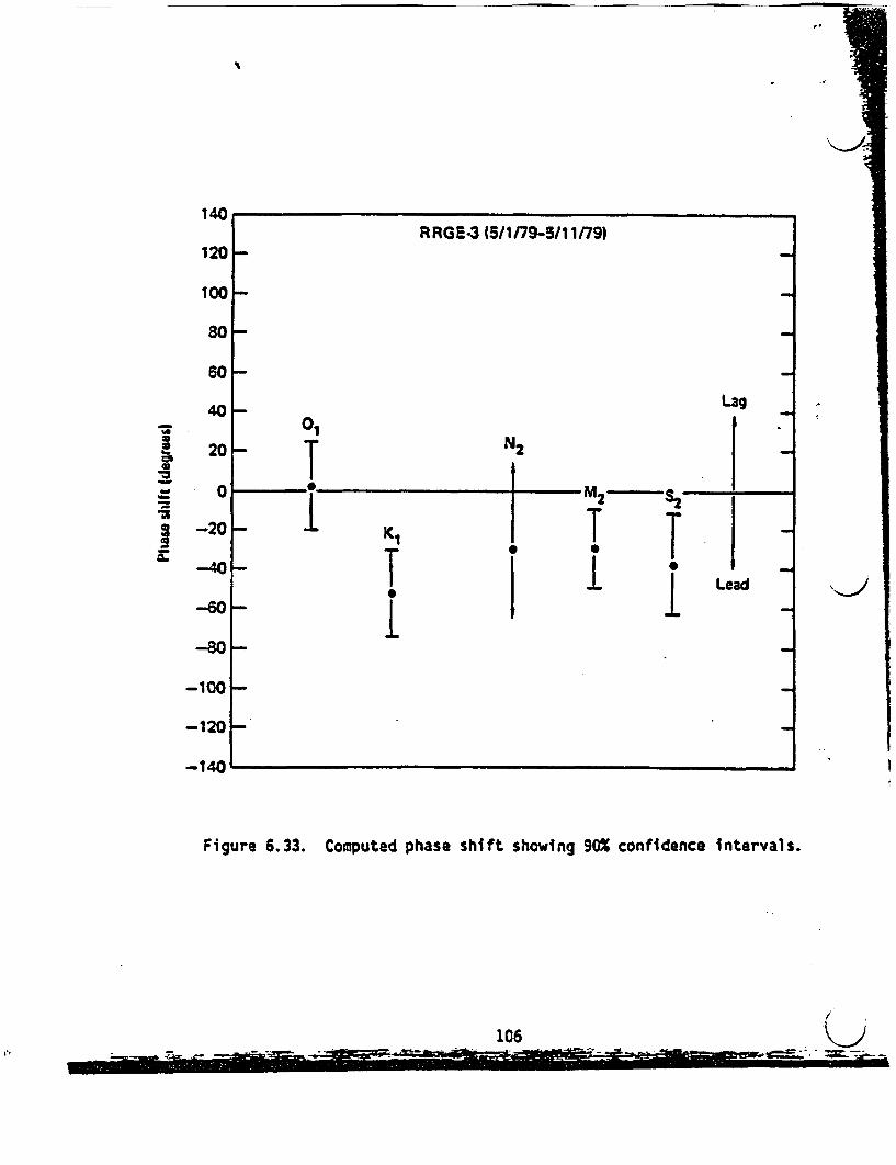
I4
*1
120
100
s0
60
40
20
0
-20
-40
--6o
-80
-100
-120
-140
IIiI
I
Figure 6.33. Computed phase shift showing 90% confidence intervals.
/06 t~106 1~
W~ w .are-wwwr - i

I
K>10-2
8 RRGI.6 (10/9/7-10/22/n8)
61 N2
41-
K1
TIia1-3
.E 8
C 6do
It 4
T
IM
S2
01
-
4I1-
21-
10 4
8
-
6 -
4
Figure 6.34. Computed tidal admittance showing 90% confidence intervals.
, I ��I �� ..
.- G-.

I
I
200
180
160
aav
140
120
100
80
60
40
20
0
-20
-40
-60
-80
Figure 6.35. Computed phase shift showing 90% confidence intervals.
108

F
K>
4
1 O-3
SM
-S
E
6
4 _
R RGI-7A (3124n-419n79)
N2
01 1 S2
T T T TI i iTT|ii.121-
10 4
8
6
LI 4
.1 Figure 6.36. Computed tidal admittance showing 9C% confidence intervals.
L
i� . W-
-%- - , -- -- --I- 4 -! -IMA*q6-rW V41 M=:Pr---t - Wd&j.-7- Ww"W"'is %I ragois . -JL -OPWAO- - �. -.L.-,I-1

140RRGI-7A 13/24n9-49n9)
120 -
100
80 _
60 -
40 N2 Lag
40 - ''2 T20T
-20 -
Lead
-80
-100
-140
Figure 6.37. Computed phase shift showing 90X confidence intervals.
110 110~~~ J

MWEMMM����
- I - K> :. '-"
4
2
10-
aat
.3
41
s
72
RRGI.78 (/1/79-8/1i9)
N2.~~~~~~~~~~~~~~~ ,
M.~~.
It TII' I
II
8
B
A'611->
IFigure 6.38. Computed tidal admittance showing 90X confidence intervals.
'. I

F-.~~~~
140
RRGI-7 (s5/1/79-/1nns120 -
100 K
01 ~~~~~~~~~~~~Lag
40 1N 2 M
figure 63 C I~-20 ± I
-40 T Lead-60 ~~~~~~~~~~~~~0
-80 1K1
-100 T-120- 1-140
Figure 6.39. Computed phase shift showing 90% confidence intervals.
112
0-�M �I

I~~~~~~~~~~~~~LA~. -
Wellhead temperature contaminated pressure at the K1 and S2 frequencies (solar
tides) is clear in several of the wells analyzed, particularly RRGI-7B.
A confined aquifer model (see Chapter III) was applied to all of the
wells for which data was available for the purpose of computing the specific
storage coefficient and porosity. This was motivated primarily by an interest
in determining the sensitivity of such a simple model for differentiating
fracture porosity from pore porosity in a reservoir that exhibits both. Table
6.1 summarizes the results of this analysis. The effective stress constant a
was taken to be 1 in the evaluation of 0 and Ss. Only the lunar O1 and MK2
tidal components were used in this and later analyses since the K1 and S2
components are of solar origin and may contain wellhead heating effects which;
will contaminate the measurement. The lunar N2 tide is typically of such'
small amplitude as to yield a large statistical uncertainty, and therefore was
not used in the analysis. The small calculated porosity and large total
compressibility determined for RRGE-1,2 and 3 are consistent with the hypothe-
sis that the primary production for these wells originates in fracture-domin-
ated production zones. Flowmeter logs and temperature logs (Stoker, et al.,
1977) as well as extensive core analyses (Dolenc, et al., 1981) for these
wells confirm this hypothesis On the other hand, RRGI-6 and RRGI-7, which are
completed in the sedimentary Salt Lake formation, have calculated porosities
of 14% and 16%. These are well within the range of porosities measured by
more conventional methods for the Salt Lake formation. Using values of perme-
ability obtained from conventional well testing to estimate the hydraulic skin
depth, it was found that the above porosity estimates are averages over dis-
tances between 2.5 and 5 km from the well. Calculated porosity for RRGE-4 was
indicative of normal primary porosity even though RRGE-4 is of similar depth
.:

V
I1,
Table 6.1
Summary of Computed Specific Storage and PorosityValues for the Raft River Geothermal Field
wall OCt (psi-') Ss (ft-') BE Ct (psi-,)
RRGE-I 3.3 x 10⁻⁷ (0X) 1.4 z 10O7 0.08 0.01 31.8 x lo-$
RRGE-2 5.1 x lo0- (02) 2.2 x 10⁻⁷ 0.18 0.04 14.2 z 10-6RGE-3 5.3 x 10⁻⁷ (u:) 2.3 X 10-? 0.24 0.05 10.6 x 10_6
RRGE-4 8.2 x 10⁻⁷ (H2) 3.5 2 10- 0.75 0.24 3.4 x 10⁻⁶RRGI-6 5.3 x 10⁻⁷ (01) 2.3 z 10- 0.69 0.14 3.8:2 106RRGI-7 1.3 x 10⁻⁶ (MO) 5.6 x 10⁻⁷ 0.30 0.16 8.1 x 10⁻⁶
114

Ah�-- I'll .. -� - -- I---,-. -- I--
ANE=195 ~~ ~fl fl
'.7 V�
�1�
II
1_1.� I
I
as RRGE-3 and also penetrates through the base of the Salt Lake formation into
the metamorphic basement complex. In 1978, RRGE-4 was deepened by 137.2 m to
a total depth of 1554.5 m. However, following recompletion neither fractures
nor improved production were observed suggesting that primary production of
RRGE-4 remained pore dominated. Core analysis (Communication from D. 0.
Enniss, Terra Tek to R. C. Stoker, EG&G Idaho, May 19, 1977) at the 640 m
depth at RRGE-4 indicates an effective porosity of 24.5%, very close to the
calculated results using the tidal response method.
A conventional injection test (Ahmed, et al., 1981) carried out in 1978
at RRGI-7 yielded a value for S L of 1.2x 10⁻³ using an assumed formation
thickness L of 548.6 m. The tidal analysis method, using the same formation
thickness, yields a value of 1.0x1O-3 for the same well. Formation thickness
for RRGE-1 and RRGE-2 is ill-defined due to the fractured and heterogeneous
nature of the production zones in these wells. However, using the open-hole
length as an effective formation thickness, the tidal response method yields a
SsL of 1.8x10⁻⁴ and 4.8x1O-4 for RRGE-1 and RRGE-2, respectively. A conven-
tional long-term interference test (Narasimhan and Witherspoon, 1977) between
these wells yielded a value of 9.4x10⁻⁴. Differences between the tidal re-
sponse method and the conventional pump test for these wells may be attributed
to differences in the nature of the applied lead and/or limitations of a
confined aquifer models for interpreting fractured formations. No comparable
conventional well test Interpretations were available for RRGE-3, RRGE-4 or
RRGI-6.
The differences in barometric efficiency and total compressibility be-
tween RRGI-6 and RRGI-7 are difficult to account for since both wells are
completed in the same formation and both have similar depth. During an injec-
tion test at RRGI-7 to 1978, a pressure response was observed RRGE-3 but noH~~ X- _H F H O W = _ -4~~~~
I
J
.& I

pressure response was observed in RRGI-6 (Allman, 1978). The report conc1d
that the most likely explanation was reservoir heterogeneity in the vicnj
of RRGI-6 and 7 allowing for a hydraulic connection between RRGI-7 and RRGF -
This observation may explain the difference in barometric efficiency and
compressibility observed between RRGI-6 and RRGI-7 and the similarity of t
parameters between RRGI-7 and RRGE-3.
The fracture orientation model was applied to tidal response data taken
at RRGE-1, RRGE-2 and RRGE-3. Dip and strike were adjusted as discussed in
Chapter III until the theoretical amplitude ratios and phase shifts of the
lunar 01 and M2 tidal pressure responses matched the measured amplitude ratios
and phase shifts. Uncertainties in the dip and strike estimates were computed
by propagating the error in computed spectral estimates of the measured fluid
pressure response as discussed in Chapter V. Figure 6.40 shows the range of
computed strike for fractures intersecting RRGE-1, RRGE-2 and RRGE-3 at the
90% confidence level. RRGE-1 and RRGE-2 have similar computed strikes which
are close to the strike of the Bridge fault. RRGE-3, however, has a comp!
strike consistent with the strike of the Narrows Structure. These resu -cs)
also suggest that, at a high confidence level, primary production at RRGE-1
and RRGE-2 comes from a set of fractures of distinctly different orientation
than the production for RRGE-3. These conclusions based on the tidal response
method are supported by water chemistry studies (Allen, et al., 1979) which
indicate that the waters at RRGE-1 and RRGE-2 originate in the Bridge fault
and are distinct from the waters at RRGE-3, which intersects the Narrows
Structure. Conventional well testing at Raft River indicates that the reser-
voir is anisotropic in the vicinity of the production wells with the major
axis of hydraulic conductivity lying roughly in the north-south direction
(Dolenc, et al., 1981).
116
K )

F igure 6.41 shows a histogram of fracture dip angles measured in core
taken within 200 -m of the sediment-crystalline basement decollement at RRGE-13.
I and RRGE-5 (Guth, et al., 1981). As indicated by the figure, the distribution
is distinctly bimodal with the majority of the fractures having a dip betweense
40° and 800. The tidal strain response analysis for dip, which is also shown
on the figure, indicates that production is from the steeply dipping set ofa n
fractures.in
Commercial borehole geophysical logging indicates that the Salt Lake.,e
formation sediments, in general, are not very permeable (Dolenc, et al.,es
1981). Also, near the base of the Salt Lake formation, considerable thermalid
alteration in the form of silica and calcite deposition has occurred (Coving-.d
ton, 1980). Therefore, the permeability contrast between the fractured pro-3f
duction zones in RRGE-1,2 and 3 and the surrounding rock can be considered
quite high. This suggests that the simple fracture model consisting of a high
permeability fracture or set of fractures within an impermeable host rock is a
reasonable first-order model for the fractured production zones at Raft River.as
.1
on
:e
t
:n4S
f /.;,. 5- A. -, ^ - -I.r ................................................................. A_ .................... . _

I
It
ARRG.1VA AYSh
___
(10 tATo
K-'
Figure 6.40. Computed fracture zone strike for RRGE-1, 2, and 3 showing 90%confidence strike sectors. Estimated strike based on surfacegeology and Landsat imagery is shown by labeled lines.
118

�iffi
.4
J@7
C
c
Figure 6.41.
-0 10- 20- 30r 40- 50 600 70- 80 900ANGLE SETWEEN CORE AXIS AND FAULT POLE
Histogram of dip angles of fractures in core taken at RRGE-1 andRRGE-S (from Guth, et al., 1981). Dip estimates based on solidearth tidal strain method (solid circles) are superimposed with90% confidence error bars.
III .
'i:- ...; .- - -- som T-.w - --=- - � --a, a_ L� --J-vr-�-M� M: . 5xswv�

Appeop- -1
Cl0-
Pe

CHAPTER VII
SUMMARY AND CONCLUSIONS
Considerable work has been carried out over the last two decades on
characterizing pore pressure response to solid earth tidal strain and baromet-
ric pressure for the case of a homogeneous and isotropic porous rock. In some
cases, these models have been used to interpret measured downhole or welihead
pressure in terms of porosity and storage. It has only been recently that the
usefulness of solid earth tidal strain for characterizing discrete fractures
in-situ has been recognized. This report presents an indirect confirmation of
the method made through comparison with other information consisting of re-
gional geology, geophysics, reservoir fluid chemistry and hydrology. In a
more direct confirmation of the method, Bower (1982) carried out tidal strain
fracture orientation analysis on shallow wells penetrating crystalline rock.
This work was directed toward evaluating the method as a technique for charac-
terizing discrete natural fractures in crystalline rock for the purpose of
subsurface containment of radioactive waste. The tidal strain results were
confirmed directly by lowering a borehole televiewer to the packed off section.
Table 7.1 shows a comparison of the orientation using solid earth tidal strain
and borehole TV. It should be emphasized that the borehole TV does not dif-
ferentiate between producing and non-producing fractures and therefore some
care must be taken in comparing these results. Furthermore, we emphasize that
the borehole televiewer yields information about fractured orientation at the
well face only. In the case of a borehole penetrating a pre-existing fracture,
the televiewer results probably reflect the fracture orientation away from the
wellbore. A stimulated fracture, however, will likely exhibit orientation at
the wellface different from the orientation of the fracture away from the well
121i

4
Table 7.1
Radioactive Waste Containment Tests -Chalk River Nuclear Laboratories, Ontario
Canada, 1982 - Borehole CR8*
Packed Off Interval (a)(Dip,
Tidal Analysis
180.8-196.7
197.6-240.9
275.3-281.1
(32°,278°)
(370,312°)
(37°,228°)
Strike)Borehole TV
(200,280), (530,2460)
(36°,3130), (540,3160)
(31°,248°)
*(1) Boreholes cased and perforated intervals packed off(2) Completion in crystalline rock - no drainage effects.
From: Internal ReportChalk River Nuclear LaboratoriesJune, 1982
122 'K-I

V
face, causing a televiewer estimation to be incorrect. The tidal method, on
the other hand, can see far from the well face. It is most encouraging that,
at every packed-off interval, there is good correlation between fractures
detected by the borehole TV and the orientation evaluated on the basis of
solid earth tidal strain. These results, along with the work carried out at
the Raft River system, indicate that the analysis of pore pressure response to
solid earth tidal strain can be an exceedingly powerful tool for determining
fracture orientation.
The advantages of the solid earth tidal strain approach for fracture
orientation analysis are many. Unlike potential field methods (e.g. resistiv-
ity, IP, magnetic proppants, etc.) and most seismic methods, the tidal strain
method has no depth limitations. As in all methods based on fluid pressure
transient analysis, the signal propagation speed is almost instantaneous when
compared with the actual fluid velocity. Therefore, the ability to predict
the migration of injected fluid in a reservoir far exceeds conventional tracer
methods which track the fluid directly. By the time tracer methods indicate a
problem associated with waste water reinjection, it is likely to be too late
to take corrective action to reduce the problem to an acceptable level.
Another advantage of the tidal strain method is the modest equipment necessary
to carry out the procedure. Welihead or downhole fluid pressure measurement
and simultaneous barometric pressure measurement over a period of a few weeks
is required. Sufficient pressure measurement resolution is obtained with
"off-the-shelf" quartz pressure gauges.
What is clearly indicated at present is the need for an expanded data
base to test more thoroughly the tidal strain response models. The method has
been applied to date only to fractures exhibiting minimal drainage to the
formation. In the work by Bower (1982), the formation permeability was in the

microdarcy range characteristic of granites. For the case of the Raft River
system, considerable thermal alteration in the form of silica and calcite
deposition in the pores had occurred in the basement Palezoic metasedimentary\ a
complex. As a result, the formation permeability was greatly reduced. One
cannot typically expect to find this optimum situation. Horizons for geother-
mal waste water reinjection are usually chosen for the opposite reason --
namely a moderately high permeability for the purpose of minimizing pumping
costs associated with reinjection. Often times, however, a large part of the
observed permeability in injection horzons can be attributed to fractures or
other high permeability channels. A good example of this is given by Elnars-
son, et al. (1975), for the case of geothermal waste water injection at the
Ahuachapin geothermal field in El Salvador. A rapid response at one of. the
wells due to the injection of a tritium tracer slug at a nearby well clearly
indicated channelling, although the total quantity of tritium recovered indi-
cated that most of the injected tritium was lost by migration into the forma-
tion. Another example of flow channelling in injection horizons has been
given in this report. The difference in barometric efficiency found between
the injection wells RRGI-6 and RRGI-7 at Raft River and the similarity between
the barometric efficiency between RRGI-7 and the production well RRGE-3 sug-
gests very strongly that the horizon chosen for reinjection at Raft River is
not isotropic. This was confirmed by a conventional pump test that indicated
a hydraulic connection between RRGE-3 and RRGI-7. The nature of this connec-
tion is not totally clear although the tidal analysis indicates that it is not
a simple non-draining fracture. The calculated connected porosity is much
more consistent with a porous injection horizon (the Salt Lake Formation) than
with a fracture.
124 K
Further testing and use of the tidal strain method in the field is clear-
ly warranted based, on the results obtained at the Raft River Geothermal Field
in Idaho and at the Chalk River Nuclear Laboratories in Canada. Several
likely candidates for future field testing of the tidal strain method are: 1)
continued work at Raft River, 2) the Fenton Hill "Hot Dry Rock" system in New
Mexico, 3) geothermal systems in the Salton Trough in Southern California, and
4) other systems in the Basin and Range province. This list contains most of
the expected geologic and hydrologic environments likely to be encountered in
future geothermal development. Potential sites, however, should not be limited
to these alone. The Raft River system is a most appropriate candidate in that
a considerable amount of knowledge has accumulated over the past decade re-
garding the regional and local structure and extent of the hydrothermal system.
The reservoir exhibits both fracture and pore porosity as well as a demon-
strated large scale hydraulic connection between the shallower pore-dominated
and deeper fracture-dominated regimes. The conclusions drawn in this report
regarding the Raft River system are based on tidal response data obtained from
conventional well tests. A field experiment tailored specifically for tidal
strain response analysis at this reservoir would no doubt improve the resolu-
tion of the data and therefore refine the conclusions reached in this report.
The Fenton Hill "Hot Dry Rock" system in New Mexico, conceived and estab-
lished by Los Alamos Scientific Laboratory (LASL), is a man-made fracture
system in deep, hot crystalline rock. Cold water is injected into the frac-
ture system via an intersecting borehole, is subsequently heated by the rock,
and the hot water is then removed from the system through a second intersect-
ing borehole. Although the long-term economic viability of this type of
system for electrical power production has yet to be verified, there is con-
siderable interest, both in the U.S. and abroad, in its space heating applica-

tions. Response of the Fenton Hill system to solid earth tidal striip 1has,been observed and is roughly 0.02-0.04 psi (personal communication, J. Al-bright, LASL). The application of tidal strain analysis to this kind ofsystem include: 1) fracture orientation analysis, necessary for successfullyintersecting the hydraulic fracture with the second borehole, 2) evaluation ofeffective fracture size, and 3) long-term fracture dilatancy due to thermo-elastic effects.
The Salton Trough is a northward extension of the Gulf of Californiaspreading center. It is an extensive region of crustal thinning, faulting,and dike injection which has resulted in many near surface thermal anomaliesof large magnitude. Considerable thermal alteration in the form of silicadeposition within many of the thermal reservoirs has resulted in the estab-lishment of fracture-dominated systems. Local on-going tectonic activityassociated withy the Pacific-North American plate interaction keeps thesefracture systems open. Environmental requirements necessitate that the pro-duced fluid, which is extremely saline (up to 300,000 ppm total dissolvedsolids), be reinjected. Reinjection is also a most important consideration inthe Imperial Valley, where ground subsidence has the potential of modifyingthe gravity-driven irrigation in this heavily agricultural area. Pore pres-sure response to solid earth tides has been observed at the' Salton Sea Geo-thermal Field (Hanson, 1979) and at the East Mesa Geothermal Field (Kanehiro,1980).
Finally, a typical "Basin and Range" type reservoir should be consideredfor the reasons that: 1) these are structurally dominated system usuallycontrolled by steeply dipping normal faults, and 2) these types of systemsdominate all others in number of occurrences and total thermal energy in theU.S. and will probably represent the future "type" system for geothermalenergy exploitation.
126

The immediate applications of earth tide analysis to geothermal reser-
voirs are three-fold: 1) as a complementary method to be used with conven-
tional pressure transient testing for characterizing the nature of the fluid
conduits (pore or fracture) within the production and injection zones, 2) as a
method for determining the structural nature (i.e. spatial orientation) of the
fluid conduits, and 3) as a method for monitoring long-term structural modifi-
cation of the reservoir due to extensive production or injection which results
in significant changes in effective stress. An example of the latter is given
in Figure 7.1. This figure shows the measured welihead pressure history of a
shut-in oil well in a Western Canadian oil field (Hanson, 1982). This partic-
ular well, which had been hydraulically fractured, produces from a formation
that is also slightly fractured. The well was shut-in shortly after nearby
wells had undergone a period of injection. It is clear from this figure that
above a certain reservoir pressure, roughly 1330 psi, the behavior of the
reservoir is as one would expect based on the results of Chapters II and III.
At a 90% confidence level, the pore pressure response to tidal strain was less
than 0.1 psi while the static pressure stayed above a critical pressure of
1300 psi. However, an interestir.g phenomena occurred as the reservoir pres-
sure dropped below this critical pressure. During this phase, the response to
tidal strain emerged and indeed was amplified over the expected response.
Figure 7.2 shows a maximum entropy amplitude spectrum of a 50 hour segment of
the data between t = 410 hours and t = 460 hours. There are two possible
explanations for the amplification. The first is that the fractures were
deforming "globally" rather than "locally". Formulation presented in Chapter
III uses a local fracture deformation expression (equation I.35) which does
not take into account the effect of fracture size on fracture dilatance. If
this were done, the observed amplication can be easily explained (Hanson,
127

1350
1340
- 1330
U,r-
% 1320L4.A:
= 1310-W 31
1300
0
Figure 7.1.
TIITE (HRS)
Measured welihead pressureCanadian oil field.
at a stimulated well in a Western
128, w

Zs,
i,- ;}
FREQUENCY (CPH)
Figure 7.2. Maximum entropyin Figure 7.1.to-t c 460 hrs.
amplitude spectrum of a portion of the data shownAnalysis is on 50 hours of data, from t 410 hrsAmplitude is in arbitrary units.
I
129

1982). The other possibility is some sort of resonance effect betweeK the
fracture elasticity and borehole storage (see for example Bodvarsson and
Bjornsson, 1976). In any event, it is clear that the response to tidal strain
was very dependent on effective stress. An understanding of this dependency
will be extremely useful for evaluating the dynamics of fracture systems
including in-situ fracture aperture-effective stress interrelationships.
The tidal amplification question is but one of several questions that
need to be answered. Others include: 1) effects of formation permeability
anisotropy and formation compressibility anisotropy on the determination of
fracture orientation, 2) connection of the primary subsurface fluid conduit
with other conduits with different hydraulic characteristics or spatial or~ien-
tation, 3) the effect of non-ideal fracture geometry on tidal response, 4)
optimization of data acquisition methods for improved resolution, and 5) the
practical feasibility of accounting for ocean loading effects in the models.
IIiI
I
I
130

'' " ' sBIBLIOGRAPHY
K.> Ahmed, U., K. Wolgemuth, A.S. Abou-Sayed, J.F. Schatz and A.H. Jones, "RaftRiver Geothermal Site: A Reinjection Study," Geothermal Res. Council,Trans., V. 4, September 1980.
Allen, C.A., R.E. Chaney, and R.E. McAtee, "Geochemical Modeling at RaftRiver," Geothermal Resources Council Trans., V. 3, 1979.
Allman, O.W., "Air Lift and Injection Testing on RRGI-7 from August 1, 1978 toAugust 3, 1978," EG&G Idaho, Internal Report, 1978.
Alsop, L.E. and J.T. Kuo, "The Characteristic Numbers of Semi-Diurnal EarthTidal Components for Various Earth Models," Ann. Geophys., V. 20, 1964.
Arditty, P., "The Earth Tide Effects on Petroleum Reservoirs; PreliminaryStudy," Stanford Geothermal Program Report SGP-TR-34, 1978.
Arditty, P. and H.J. Ramey, "Response of a Closed Well-Reservoir System toStress Induced by Earth Tides," SPE Paper 7484, Houston, Texas, 1978.
Armstrong, R.L., "Mantled Gneiss Domes in the Albion Range, Southern Idaho,"Geol. Soc. Am. Bull., 79, p. 1295, 1968.
Beaumont, C. and J. Berger, uAn Analysis of Tidal Strain Observations from theUnited States of America: I. The Laterally Homogeneous Tide," Bull.Seis. Soc. Am., 65, 6, 1975.
Berger, J. and F. Wyatt, "Some Observations of Earth Strain Tides in Californ-ia," Phil. Trans. R. Soc. Lond. A., 274, 1973.
Berger, J. and C. Beaumont, "An Analysis of Tidal Strain Observations from theUnited States of America: II, The Inhomogeneous Tide," Bull. Seis. Soc.Am., 66, 6, 1976.
Blot, M.A., "General Theory of Three-Dimensional Consolidation," J. App.Phys., 12, 1941.
Blair, D., "Fourier Contamination of a Finite Length of Data in Tidal Analy-sis," Geophys. J.R. astr. Soc., 59, 1979.
Bodvarsson, G., "Confined Fluids as Strain Meters," J. Geophys. Res., 75, 14,1970.
Bodvarsson, G. and A. Bjornsson, "Hydroelastic Cavity Resonators," Jbkull, 26,1976.
Bodvarsson, G. and J.M. Hanson, "Geothermal Reservoir Testing Based on Signalsof Tidal Origin," Proc. 4th Workshop on Geothermal Reservoir Engineering,Stanford Univ., 1978.
131 A

Bower, D.R., Fracture Parameters From the Interpretation of Well Tides." ,.,,Geophys. Res., 1983 (in press). ' *
Bower, D.R. and K.C. Heaton, "Response of an Aquifer Near Ottawa to TidalForcing and the Alaskan Earthquake of 1964," Can. J. Earth Sci., 15, 3, X1978.
Bredehoeft, J.D., "Response of Well-Aquifer Systems to Earth Tides," J. Geo-phys. Res., 72, 12, 1967.
Sullen, K.E., The Earth's Density, John Wiley & Sons, 1975.
Chapman, S. and K.C. Westfold, "Comparison of the Annual Mean Solar and LunarAtmospheric Tides in Barometric Pressure, as Regards Their WorldwideDistribution of Amplitude and Phase," Jour. Atmos. and Terres. Phys., 8,1956.
Cinco-Ley, H. and F. Samaniego-V, "Transient Pressure Analysis for FracturedWells," J. Pet. Tech., pp. 1749-1766, 1981.
Compton, R.R., "Geologic Map of the Yost Quadrangle, Box Elder County, Utah,and Cassia County, Idaho," U.S.G.S. Misc. Geol. Inv. Map 1-672, 1972.
Covington, H.R., "Subsurface Geology of the Raft River Geothermal Area, Idaho,"Geothermal Resources Council Trans., V. 4, 1980.
DeWeist, R.J.M.,. "On the Storage Coefficient and the Equations of GroundwaterFlow," J. Geophys. Res., 71, 4, 1966.
Oolenc, M.R., L.C. Hull, S.A. Mizell, B.F. Russell, P.A. Skiba, J.A. Strawn,and J.A. Tullis, "Raft River Geosciences Case Study," EG&G Idaho, ReportEGG-2125, V. I, II, 1981.
Duguid, J.O. and P.C.Y. Lee, "Flow in Fractured Porous Media," Water Res.Research, 13, 3, 1977.
Einarsson, S., A. Vides, R., and G. Cuellar, "Disposal of Geothermal WasteWater by Reinjection," Proc. 2nd U.N. Symp. on the Dev. and Use of Geo-thermal Res., San Francisco, May 1975.
Farrell, W.E., "Global Calculations of Tidal Loading," Nat. Phys. Sci., 238,1972.
Farrell, W.E., "Earth Tides," Rev. Geophys. and Space Phys., 17, 6, 1979.
Felix, C.E., "Geology of the Eastern Part of the Raft River Range, Box ElderCounty, Utah," in Guidebook to the Geoloqy of Parts of Northwestern Utah,Utah Geol. Soc., 11, pp. 76-97, 1956.
George, W.O. and F.E. Romberg, "Tide-Producing Forces and Artesian Pressures,"Trans. Am. Geophys. Union, 32, 3, 1951.
Godin, G., The Analysis of Tides, Univ. of Toronto Press, 1972.

Goldman, S., Information Theory. Dover Publications, 19685
Guth, L.R. R.L. Brahn, 'and S.L. Beck, "Fault and Joint Geometry at Raft RiverGeothermal Area, Idaho," Univ. of Utah, Report OOE-ID-12079-41, 19i1.
Hanson, J.M., "Tidal Pressure Response Well Testing at the Salton Sea Geother-mal Field,_California and Raft River, Idaho, Proc. 5th Workshop on Geo-thermal Reservoir Engineering, Stanford Univ., 1979.
Hanson, J.M. and L.B. Owen, "Fracture Orientation Analysis by the Solid EarthTidal Strain Method," SPE Paper 11070, New Orleans, LA, 1982.
Hanson, J.M., uIn-Situ Fracture Characterization - A Hew Approach Using Multi-Frequency Flow Testing," Proc. 24th U.S. Symposium on Rock Mechanics,Texas A&M Univ., June 20-23, 1983 (in press).
Harrison, J.C., N.F. Ness, I.M. Longman, R.F.S. Forbes, E.A. Kraut, and L.B.Slichter, "Earth-Tide Observations!Made During the International Geophys-ical Year," J. Geophys. Res., 68, 5, 1963.
Harrison, J.C., "New Computer Programs for the Calculation of Earth Tides,"NOAA, Univ. of Colorado, CIRES, 1971.
Harrison, J.C., "Cavity and Topographic Effects in Tilt and Strain Measure-ment," J. Geophys. Res., 81, 2, 1976.
Jacob, C.E., "On the Flow of Water in ad Elastic Artesian Aquifer," Trans. An.Geophys. Union, Part 2, 1940.
Kanehiro, B.Y., "The Response of Aquifers to the Earth Tides," M.S. Thesis,i w Univ. of California, Berkeley, 1980.
King, G.C.P. and R.G. Bilham, "Strain Measurement Instrumentation and Tech-nique," Phil. Trans. R. Soc. Lon. A., 274, 1973.
Khorosheva, V., 'Effect of the Atmospheric Pressure on the Tilting of theEarth's Surface," Izv., Geophys. Ser., 1958.
Kuo, J.T., R.C. Jachens, M. Ewing, and G. White, "Transcontinental TidalGravity Profile Across the United States, Science, 168, 1970.
Lambert, A., "The Response of the Earth to Loading by the Ocean Tides aroundNova Scotia," Geophys. J. R. astr. Soc., 19, 1970.
Longman, I.M., "Formulas for Computing the Tidal Accelerations Due to the Moonand the Sun," J. Geophys. Res., 64, 12, 1959.
Mabey, D.R., D.B. Cooper, J.E. O'Donnell, and C.W. Wilson, "ReconnaissanceGeophysical Studies of the Geothermal System in Southern Raft RiverValley, Idaho," Geophysics, 43, 7, 1978.
Major, M.W., G.H. Sutton, J. Oliver, and R. Metsger, "On Elastic Strain of theEarth in the Period Range 5 seconds to 100 hours," Bull. Seis. Soc. Am.,54, 1, 1964.
133
Marine, I.W., "Water Level Fluctuations Due to Earth Tides in a Well PumpingFrom Slightly Fractured Crystalline Rock," Water Res. Research, ,1975.
Melchior, P., The Earth Tides, Pergamon, 1966.
Melchior, P., The Tides of the Planet Earth, Pergamon, 1978.
Morland, L.W., "Earth Tide Effects on Flows in Horizontal Permeable ElasticLayers Connected to Wells," Geophys. J. R. astr. Soc., 51, 1977.
Munk, W. and K. Hasselmann, "Super-Resolution of Tides," Studies on Oceanog-raphy, pp. 339-344, 1964.
Narasimhan, T.N. and P.A. Witherspoon, "Reservoir Evaluation Tests on RRGE-1and RRGE-2, Raft River Geothermal Project, Idaho," Univ. of Calif. ReportLBL-5958, 1977.
Nur, A. and J.D. Byerlee, "An Exact Effective Stress Law for Elastic Deforma-tion of Rock with Fluids," J. Geophys. Res., 76, 26, 1971.
Prothero, W.A. and J.M. Goodkind, "Earth-Tide Measurements with the Supercon-ducting Gravimeter," J. Geophys. Res., 77, 5, 1972.
Rhoads, G.H., Jr., "Determination of Aquifer Parameters from Well Tides," M.S.Thesis, Virginia Polytechnic Institute and State University, 1976.
Rice, J.R. and M.P. Cleary, "Some Basic Stress Diffusion Solutions for Fluid-Saturated Elastic Porous Media with Compressible Constituents," Rev.Geophys. Space Phys., 14, 1976.
Richardson, R.M., "Tidal Fluctuations of Water Level Observed in Wells in EastTennessee," Trans. Am. Geophys. Union, 37, 4, 1956.
Robinson, E.S. and R.T. Bell, "Tides in Confined Well-Aquifer Systems," J.Geophys. Res., 76, 8, 1971.
Robinson, T.W., "Earth-Tides Shown by Fluctuations of Water-Levels in Wells inNew Mexico and Iowa," Trans. Am. Geophys. Union, Reports and Papers,Hydrology, 1939.
Rosato, N.D., C.O. Bennett, A.C. Reynolds, and R. Raghavan, "Analysis ofShort-Time Buildup Data for Finite-Conductivity Fractures," J. Pet.Tech., pp. 2413-2422, 1982.
Snow, D.R., "Fracture Deformation and Changes of Permeability and Storage UponChanges in Fluid Pressure," Quart. Colo. Sch. of Mines, 63, 1, 1968.
Stehfest, H., "Algorithm 368," Collected Algorithms from CACM, 1969.
Sterling, A. and E. Smets, "Study of Earth Tides, Earthquakes and TerrestrialSpectroscopy by Analysis of the Level Fluctuations in a Borehole atHeibaart (Belgium)," Geophys. J. R. astr. Soc., 23, 1971.
_~~~~~~~~~~~~~~~ .! C pt-ol

- k W l l s s s in~ -.
Stoker, R.C., D. Goldman, and J.F. Kunze, 'Deducing Production Zones From WellLogs," Geothermal Resources Council Trans., V. 1, 1977.
Takeuchi, H., "On the Earth Tide of the Compressible Earth of Variable Densityand Elasticity," Trans. Am. Geophys.,Union, 31, 5, 1950.
Tanaka, T., "On the Effect of Atmospheric Pressure Upon Ground Tilt," Bull.Disas. Prey. Res. Inst., Kyoto Univ., 18, 2, 1968 (abstract).
Tanaka, T., "On the Effect of Atmospheric Pressure Upon Ground Tilt," Bull.Disas. Prey. Res. Inst., Kyoto Univ., 18, 2, 1968.
Trubytsyn, A.P. and A.V. Makalin, "Deformations of the Earth's Crust Due toAtmospheric Cyclones," Izv., Earth Physics, 5, 1976.
Urmantsev, F.M., "Barometric and Surface Inclinations and Their Effect on theDetermination of Contemporary Vertical Movements of the Earth's Crust bythe Geodetic Method," Izv., Earth Physics, 6, 1970.
Urmanstev, F.M., "An Estimate of the Effect of the Diurnal Variations ofAtmospheric Pressure on Gravimeter and Tiltmeter Readings on PreciseLeveling Work," Izv., Earth Physics, 3, 1975.
Van der Kamp, G. and J.E. Gale, "Theory of Earth Tide and Barometric Effectsin Porous Formations with Compressible Grains," Water Res. Research, (inpress), 1983.
Witherspoon, P.A., T.N. Narasimhan, and D.G. McEdwards, "Results of Interfer-ence Tests from Two Geothermal Reservoirs," J. Pet. Tech., Jar., 1978.
Zschau, J., "The Influence of Air Pressure Variations on Tilt MeasurementsWith the Askania Borehole Pendulum at the Station Kiel-Rehmsberg," Proc.of the 7th Symposium on Earth Tides, Edited by G. Szadeczky-Kardoss,Akademia! Kiado, Budapest, 17b6.
I IU. S. Governenrt Printing Off$ 19iI 4/0-587.002/24012
135