evaluation of sub- and supercritical rankine cycle
TRANSCRIPT

i
Evaluation of sub- and supercritical
Rankine cycle optimisation criteria
PJ Pieters
20275234
B.ENG (Mechanical Engineering)
Dissertation submitted in fulfilment of the requirements for the
degree Magister in Mechanical Engineering at the
Potchefstroom Campus of the North-West University
Supervisor: Prof C Storm
April 2016
ii
Declaration I Petrus Johannes Pieters (8704285127089) hereby declare that the work done in this
dissertation is a presentation of my own work (research and programming). Wherever I made
use of the work of others, I made every effort to indicate this clearly. Some of the information
contained in this dissertation has been gained from various journal articles; text books etc.,
and has been referenced accordingly.
The work was done under the guidance of Professor Chris Storm, at the North-West
University (Potchefstroom Campus).
29 April 2016
________________________ ____________
PJ Pieters Date
In my capacity as supervisor of this dissertation, I certify that the above statements are true to
the best of my knowledge.
29 April 2016
________________________ ____________
Prof CP Storm Date

iii
Abstract The main purpose for this study has been to model an advanced real Rankine cycle for sub
and super-critical boilers with all the components as encountered in the industry
mathematically and to optimise each cycle.
First the Development of the Rankine cycle is illustrated from the most effective theoretical
Carnot cycle through to an advanced ideal Rankine cycle with feed water heating and
compared to each other by means of the results obtained from EES. After the Ideal Rankine
cycle with all the relevant components had been programmed and discussed the Cycle was
further developed into an advanced real Rankine cycle.
The Advanced real Rankine cycle consists of Superheat, Reheat, two high-pressure feed
heaters, a de-aerator, three (super-critical) or four (sub-critical) low-pressure feed heaters, a
condenser, a condensate extraction pump and one main feed water pump. The real cycle
made provision for pressure losses, efficiencies, steam attemperation and temperature losses.
The following were optimised to get the maximum efficiency and net mechanical work for each
cycle:
Feed pump maximum pressure
High pressure turbine expansion
Two high pressure feed water heaters
The de-aerator
Three or four low pressure feed water heaters
The study touches on low pressure turbine outlet steam quality, but keeps it constant through
the optimisation stages.
To finish off, a comparison between sub- and super-critical Rankine cycles was done before
and after optimisation.

iv
Acknowledgements I would like to gratefully and sincerely thank my supervisor Prof Chris Storm for his guidance,
understanding, patience and effort during my graduate studies at North West University. His
mentorship was of most importance in my study and my long term career goals. It was a
privilege to work with him and learn so many things from his experience.
I would also like to say a special thanks to Mr Cronier van Niekerk for his help and knowledge
with programming on EES. He taught me a lot that would be helpful throughout my career.
I want to thank my co-worker and friend Mr Pieter Labuschagne for his help during my studies.
He was always helpful in every way.
I want to give a special thanks to my girlfriend for her support, encouragement, quiet patience
and help during my studies.
I would like to give my gratitude to my employer Carab Tekniva for supporting me in further
studies and all the understanding shown and leave granted.
Finally and most importantly I would like to thank Eskom Holdings SOC Ltd for letting me use
all the data to execute and compare my results during the programming.

v
Table of contents:
Declaration ........................................................................................................................................................ ii
Abstract ........................................................................................................................................................... iii
Acknowledgements........................................................................................................................................... iv
Table of contents: ............................................................................................................................................. v
Table of figures: ...............................................................................................................................................viii
Table of Tables: .............................................................................................................................................. xvii
Table of Symbols: .......................................................................................................................................... xxiii
1. Introduction ............................................................................................................... 1
1.1. Background ................................................................................................................................ 1
1.2. Problem statement ...................................................................................................................... 1
1.3. Objectives ................................................................................................................................... 2
1.4. Experimental procedure and research methodology .................................................................. 2
1.5. Assumptions and limitations ....................................................................................................... 3
1.6. Dissertation summary ................................................................................................................. 5
2. Literature survey and existing technology ................................................................. 6
2.1. Rankine cycle ............................................................................................................................. 6
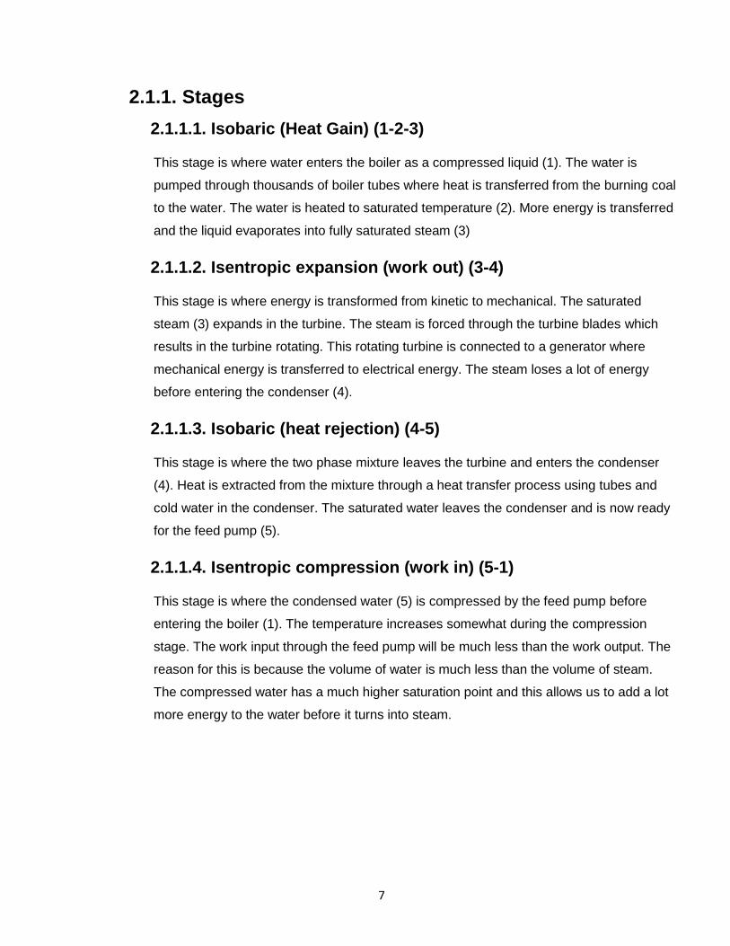
2.1.1. Stages .............................................................................................................................................. 7
2.2. Sub-critical Rankine cycle plant layout (Kriel) ............................................................................. 8
2.3. Super-critical Rankine cycle plant layout (Medupi) ................................................................... 10
2.4. Optimisation of Rankine cycle .................................................................................................. 11
2.4.1. Efficiency optimisation .................................................................................................................... 11
2.4.2. Multi-objective optimisation ............................................................................................................. 12
3. Development of the Rankine cycle and optimisation ............................................... 13
3.1. Development of Rankine cycle ................................................................................................. 13
3.1.1. Carnot cycle .................................................................................................................................... 13
3.1.2. Basic Rankine cycle ........................................................................................................................ 15
3.1.3. Rankine cycle with superheat ......................................................................................................... 16
3.1.4. Rankine cycle with superheat and reheat........................................................................................ 17
3.1.5. Rankine cycle with superheat, reheat and feed water heating ......................................................... 19
3.2. Steam quality at turbine outlet .................................................................................................. 20
vi
3.2.1. Influence of boiler pressure ............................................................................................................. 20
3.2.2. Influence by maximum temperature ................................................................................................ 21
3.2.3. Influence by high pressure turbine expansion ................................................................................. 22
3.3. Natural vs forced circulation boilers .......................................................................................... 23
3.3.1. Natural circulation (steam drum boilers) .......................................................................................... 23
3.3.2. Forced circulation (once through boilers) ........................................................................................ 24
3.4. Difference between sub- and super-critical Rankine cycles ...................................................... 26
3.4.1. Sub-critical Rankine cycle ............................................................................................................... 26
3.4.2. Super-critical Rankine cycle ............................................................................................................ 27
4. Rankine cycle programming methodology to enable optimisation ........................... 28
4.1. Rankine cycle efficiency ........................................................................................................... 28
4.1.1. Increasing boiler pressure ............................................................................................................... 28
4.1.2. Increasing boiler temperature ......................................................................................................... 29
4.1.3. Lowering the condenser pressure ................................................................................................... 30
5. Programming of sub- and supercritical Rankine cycles ........................................... 31
5.1. Sub-critical Rankine cycle ......................................................................................................... 31
5.1.1. Rankine cycle without optimisation ................................................................................................. 31
5.1.2. Optimisation of the sub-critical Rankine cycle ................................................................................. 44
5.2. Super-critical Rankine cycle ..................................................................................................... 47
5.2.1. Rankine cycle without optimisation ................................................................................................. 47
5.3. Sub- and super-critical Rankine cycle optimisation ................................................................... 48
5.3.1. Optimisation method 1 .................................................................................................................... 48
5.3.2. Optimisation method 2 .................................................................................................................... 48
6. Results of sub- and super-critical Rankine cycles ................................................... 50
6.1. Sub-critical optimisation results ................................................................................................ 50
6.1.1. Sub-critical cycle without optimisation ............................................................................................. 50
6.1.2. Sub-critical cycle optimisation – first method ................................................................................... 52
6.1.3. Sub-critical cycle optimisation – second method ............................................................................. 78
6.1.4. Adjustments after sub-critical cycle was optimised ........................................................................ 104
6.1.5. Summary of sub-critical results ..................................................................................................... 105
6.2. Super-critical optimisation results ........................................................................................... 106
6.2.1. Super-critical cycle without optimisation ........................................................................................ 106

vii
6.2.2. Super-critical cycle optimisation – first method ............................................................................. 108
6.2.3. Super-critical cycle optimisation – second method ........................................................................ 131
6.2.4. Adjustments to the final optimised cycles for super-critical ............................................................ 154
6.3. Sub-critical vs super-critical .................................................................................................... 156
6.3.1. Before optimisation ....................................................................................................................... 156
6.3.2. After optimisation .......................................................................................................................... 157
7. Conclusion and recommendations ........................................................................ 158
7.1. Conclusions ............................................................................................................................ 158
7.2. Recommendations .................................................................................................................. 160
8. References ........................................................................................................... 161
9. Appendix .............................................................................................................. 165
9.1. Appendix A ............................................................................................................................. 165
9.1.1. Material development.................................................................................................................... 165
9.2. Appendix B ............................................................................................................................. 168
9.2.1. Sub-critical boilers ........................................................................................................................ 168
9.2.2. Super-critical boilers ..................................................................................................................... 169
9.3. Appendix C: ............................................................................................................................ 171
9.3.1. Boiler history and development ..................................................................................................... 171
viii
Table of figures:
Figure 1: Rankine cycle process flow diagram ......................................................................................................... 6
Figure 2: Illustration of Kriel Power Station flow diagram ......................................................................................... 9
Figure 3: Illustration of Medupi Power Station flow diagram ....................................................................................10
Figure 4: Cycle efficiency plotted against feed heater tap off pressure....................................................................11
Figure 5: Cycle efficiency, net mechanical work and local minimum/maximum line plotted against steam
extraction mass flow ...........................................................................................................................12
Figure 6: T-s diagram to illustrate the Carnot cycle .................................................................................................14
Figure 7: T-s diagram to illustrate the Basic Rankine cycle .....................................................................................15
Figure 8: T-s diagram to illustrate the Rankine cycle with superheat .......................................................................16
Figure 9: T-s diagram for the Rankine cycle with superheat and reheat ..................................................................17
Figure 10: T-s diagram for the Rankine cycle with superheat, reheat and feed water heating .................................19
Figure 11: T-s diagram with different pressure lines and the effect of it on the low pressure turbine outlet
steam quality. .....................................................................................................................................20
Figure 12: T-s diagram with different temperature lines and the effect of it on the low pressure turbine
outlet steam quality. ...........................................................................................................................21
Figure 13: T-s diagram to illustrate the high pressure turbine expansion and the effect of it on the low
pressure turbine outlet steam quality ..................................................................................................22
Figure 14: Illustration of the flow for drum boilers (power) .......................................................................................23
Figure 15: Illustration of the flow for once through boilers (power) ..........................................................................24
Figure 16: Illustration of a sub-critical Rankine T-s diagram ....................................................................................26
Figure 17: Illustration of a super-critical Rankine cycle T-s diagram ........................................................................27
Figure 18: Effect of boiler pressure on net mechanical work (Laure, 2011) .............................................................28
Figure 19: Effect of temperature on net mechanical work (Laure, 2011) .................................................................29
Figure 20: Effect of lowering the condenser pressure on net mechanical work (Laure, 2011) .................................30
Figure 21: Enthalpy plotted against entropy to illustrated the effect of efficiency of a pump (An analysis of
a thermal power plant working on a Rankine cycle : A theoretical investigation, 2008) .......................32
Figure 22: Illustration of the efficiency effect of the low pressure turbine on the Rankine cycle ...............................33
Figure 23: Illustration of the efficiency effect of the intermediate pressure turbine on the Rankine cycle .................35
Figure 24: Enthalpy plotted against entropy to illustrate the effect of efficiency on a pump (An analysis of a
thermal power plant working on a Rankine cycle: A theoretical investigation, 2008) ...........................37
Figure 25: Illustration of the efficiency effect of the intermediate pressure turbine on the Rankine cycle .................40
Figure 26: Illustration of the efficiency effect of the intermediate pressure turbine on the Rankine cycle .................42
Figure 27: Illustration of the efficiency effect of the low pressure turbine on the Rankine cycle ...............................43

ix
Figure 28: Illustration of the efficiency effect of the intermediate pressure turbine on the Rankine cycle .................47
Figure 29: T-s diagram after programmed on EES for sub-critical cycle before any optimisation ............................51
Figure 30: Illustration of Kriel power station plant layout .........................................................................................51
Figure 31: Cycle efficiency, net mechanical work and the factor line plotted against boiler feed pump
discharge pressure (1st method, 1st run) ...........................................................................................52
Figure 32: Cycle efficiency, net mechanical work and the factor line plotted against boiler feed pump
discharge pressure (Zoomed in) (1st method, 1st run) .......................................................................52
Figure 33: Cycle efficiency, net mechanical work and the factor line plotted against the high pressure
turbine expansion pressure (1st method, 1st run) ...............................................................................53
Figure 34: Cycle efficiency, net mechanical work and the factor line plotted against the high pressure
heater 6 steam tap off pressure (1st method, 1st run) ........................................................................54
Figure 35: Cycle efficiency, net mechanical work and the factor line plotted against the de-aerator steam
bled off pressure (1st method, 1st run) ...............................................................................................55
Figure 36: Cycle efficiency, net mechanical work and the factor line plotted against low pressure heater 4
steam bled off pressure (1st method, 1st run) ....................................................................................56
Figure 37: Cycle efficiency, net mechanical work and the factor line plotted against low pressure heater 3
steam bled off pressure (1st method, 1st run) ....................................................................................57
Figure 38: Cycle efficiency, net mechanical work and the factor line plotted against low pressure heater 2
steam bled off pressure (1st method, 1st run) ....................................................................................58
Figure 39: Cycle efficiency, net mechanical work and the factor line plotted against low pressure heater 1
steam bled off pressure (1st method, 1st run) ....................................................................................59
Figure 40: Cycle efficiency, net mechanical work and the factor line plotted against boiler feed pump
discharge pressure (1st method, 2nd run) ..........................................................................................60
Figure 41: Cycle efficiency, net mechanical work and the factor line plotted against boiler feed pump
discharge pressure (zoomed in) (1st method, 2nd run) ......................................................................60
Figure 42: Cycle efficiency, net mechanical work and the factor line plotted against the high pressure
turbine expansion pressure (1st method, 2nd run) .............................................................................61
Figure 43: Cycle efficiency, net mechanical work and the factor line plotted against the high pressure
heater 6 steam tap off pressure (1st method, 2nd run) .......................................................................62
Figure 44: Cycle efficiency, net mechanical work and the factor line plotted against the de-aerator steam
bled off pressure (1st method, 2nd run) ..............................................................................................63
Figure 45: Cycle efficiency, net mechanical work and the factor line plotted against low pressure heater 4
steam bled off pressure (1st method, 2nd run) ...................................................................................64
x
Figure 46: Cycle efficiency, net mechanical work and the factor line plotted against low pressure heater 3
steam bled off pressure (1st method, 2nd run) ...................................................................................65
Figure 47: Cycle efficiency, net mechanical work and the factor line plotted against low pressure heater 2
steam bled off pressure (1st method, 2nd run) ...................................................................................66
Figure 48: Cycle efficiency, net mechanical work and the factor line plotted against low pressure heater 1
steam bled off pressure (1st method, 2nd run) ...................................................................................67
Figure 49: Cycle efficiency, net mechanical work and the factor line plotted against boiler feed pump
discharge pressure (1st method, 3rd run) ...........................................................................................68
Figure 50: Cycle efficiency, net mechanical work and the factor line plotted against boiler feed pump
discharge pressure (zoomed in) (1st method, 3rd run) .......................................................................68
Figure 51: Cycle efficiency, net mechanical work and the factor line plotted against the high pressure
turbine expansion pressure (1st method, 3rd run) ..............................................................................69
Figure 52: Cycle efficiency, net mechanical work and the factor line plotted against the high pressure
heater 6 steam tap off pressure (1st method, 3rd run) ........................................................................70
Figure 53: Cycle efficiency, net mechanical work and the factor line plotted against the de-aerator steam
bled off pressure (1st method, 3rd run) ..............................................................................................71
Figure 54: Cycle efficiency, net mechanical work and the factor line plotted against low pressure heater 4
steam bled off pressure (1st method, 3rd run) ....................................................................................72
Figure 55: Cycle efficiency, net mechanical work and the factor line plotted against low pressure heater 3
steam bled off pressure (1st method, 3rd run) ....................................................................................73
Figure 56: Cycle efficiency, net mechanical work and the factor line plotted against low pressure heater 2
steam bled off pressure (1st method, 3rd run) ....................................................................................74
Figure 57: Cycle efficiency, net mechanical work and the factor line plotted against low pressure heater 1
steam bled off pressure (1st method, 3rd run) ....................................................................................75
Figure 58: Cycle efficiency, net mechanical work and the factor line plotted against boiler feed pump
discharge pressure (1st method, 4th run) ...........................................................................................76
Figure 59: Cycle efficiency, net mechanical work and the factor line plotted against boiler feed pump
discharge pressure (Zoomed in) (1st method, 4th run) .......................................................................76
Figure 60: Cycle efficiency, net mechanical work and the factor line plotted against the high pressure
turbine expansion pressure (1st method, 4th run) ..............................................................................77
Figure 61: Cycle efficiency, net mechanical work and the factor line plotted against boiler feed pump
discharge pressure (2nd method, 1st run) ..........................................................................................78
Figure 62: Cycle efficiency, net mechanical work and the factor line plotted against boiler feed pump
discharge pressure (zoomed in) (2nd method, 1st run) ......................................................................78

xi
Figure 63: Cycle efficiency, net mechanical work and the factor line plotted against the high pressure
heater 6 steam tap off pressure (2nd method, 1st run) .......................................................................79
Figure 64: Cycle efficiency, net mechanical work and the factor line plotted against the high pressure
turbine expansion pressure (2nd method, 1st run) .............................................................................80
Figure 65: Cycle efficiency, net mechanical work and the factor line plotted against low pressure heater 1
steam bled off pressure (2nd method, 1st run) ...................................................................................81
Figure 66: Cycle efficiency, net mechanical work and the factor line plotted against low pressure heater 2
steam bled off pressure (2nd method, 1st run) ...................................................................................82
Figure 67: Cycle efficiency, net mechanical work and the factor line plotted against low pressure heater 3
steam bled off pressure (2nd method, 1st run) ...................................................................................83
Figure 68: Cycle efficiency, net mechanical work and the factor line plotted against low pressure heater 4
steam bled off pressure (2nd method, 1st run) ...................................................................................84
Figure 69: Cycle efficiency, net mechanical work and the factor line plotted against the de-aerator steam
bled off pressure (2nd method, 1st run) ..............................................................................................85
Figure 70: Cycle efficiency, net mechanical work and the factor line plotted against boiler feed pump
discharge pressure (2nd method, 2nd run) .........................................................................................86
Figure 71: Cycle efficiency, net mechanical work and the factor line plotted against boiler feed pump
discharge pressure (zoomed in) (2nd method, 2nd run) .....................................................................86
Figure 72: Cycle efficiency, net mechanical work and the factor line plotted against the high pressure
heater 6 steam tap off pressure (2nd method, 2nd run) ......................................................................87
Figure 73: Cycle efficiency, net mechanical work and the factor line plotted against the high pressure
turbine expansion pressure (2nd method, 2nd run) ............................................................................88
Figure 74: Cycle efficiency, net mechanical work and the factor line plotted against low pressure heater 1
steam bled off pressure (2nd method, 2nd run) ..................................................................................89
Figure 75: Cycle efficiency, net mechanical work and the factor line plotted against low pressure heater 2
steam bled off pressure (2nd method, 2nd run) ..................................................................................90
Figure 76: Cycle efficiency, net mechanical work and the factor line plotted against low pressure heater 3
steam bled off pressure (2nd method, 2nd run) ..................................................................................91
Figure 77: Cycle efficiency, net mechanical work and the factor line plotted against low pressure heater 4
steam bled off pressure (2nd method, 2nd run) ..................................................................................92
Figure 78: Cycle efficiency, net mechanical work and the factor line plotted against the de-aerator steam
bled off pressure (2nd method, 2nd run) ............................................................................................93
Figure 79: Cycle efficiency, net mechanical work and the factor line plotted against boiler feed pump
discharge pressure (2nd method, 3rd run)..........................................................................................94

xii
Figure 80: Cycle efficiency, net mechanical work and the factor line plotted against boiler feed pump
discharge pressure (zoomed in) (2nd method, 3rd run) ......................................................................94
Figure 81: Cycle efficiency, net mechanical work and the factor line plotted against the high pressure
heater 6 steam tap off pressure (2nd method, 3rd run).......................................................................95
Figure 82: Cycle efficiency, net mechanical work and the factor line plotted against the high pressure
turbine expansion pressure (2nd method, 3rd run) .............................................................................96
Figure 83: Cycle efficiency, net mechanical work and the factor line plotted against low pressure heater 1
steam bled off pressure (2nd method, 3rd run) ...................................................................................97
Figure 84: Cycle efficiency, net mechanical work and the factor line plotted against low pressure heater 2
steam bled off pressure (2nd method, 3rd run) ...................................................................................98
Figure 85: Cycle efficiency, net mechanical work and the factor line plotted against low pressure heater 3
steams bled off pressure (2nd method, 3rd run) .................................................................................99
Figure 86: Cycle efficiency, net mechanical work and the factor line plotted against low pressure heater 4
steam bled off pressure (2nd method, 3rd run) ................................................................................. 100
Figure 87: Cycle efficiency, net mechanical work and the factor line plotted against the de-aerator steam
bled off pressure (2nd method, 3rd run) ........................................................................................... 101
Figure 88: Cycle efficiency, net mechanical work and the factor line plotted against boiler feed pump
discharge pressure (2nd method, 4th run) ........................................................................................ 102
Figure 89: Cycle efficiency, net mechanical work and the factor line plotted against boiler feed pump
discharge pressure (zoomed in) (2nd method, 4th run) .................................................................... 102
Figure 90: Cycle efficiency, net mechanical work and the factor line plotted against the high pressure
turbine expansion pressure (2nd method, 4th run) ........................................................................... 103
Figure 91: Sub-critical plant layout with steam flows, after high pressure heater 6 was taken out ......................... 104
Figure 92: Current super-critical Rankine cycle before any optimisation ............................................................... 107
Figure 93: Plant layout at Medupi power station (super-critical) ............................................................................ 107
Figure 94: Cycle efficiency, net mechanical work and the factor line plotted against boiler feed pump
discharge pressure (1st method, 1st run) ......................................................................................... 108
Figure 95: Cycle efficiency, net mechanical work and the factor line plotted against boiler feed pump
discharge pressure (zoomed in) (1st method, 1st run)...................................................................... 108
Figure 96: Cycle efficiency, net mechanical work and the factor line plotted against the high pressure
turbine expansion pressure (1st method, 1st run) ............................................................................. 109
Figure 97: Cycle efficiency, net mechanical work and the factor line plotted against the high pressure
heater 6 steam tap off pressure (1st method, 1st run) ...................................................................... 110

xiii
Figure 98: Cycle efficiency, net mechanical work and the factor line plotted against the de-aerator steam
bled off pressure (1st method, 1st run) ............................................................................................. 111
Figure 99: Cycle efficiency, net mechanical work and the factor line plotted against low pressure heater 3
steam bled off pressure (1st method, 1st run) .................................................................................. 112
Figure 100: Cycle efficiency, net mechanical work and the factor line plotted against low pressure heater 2
steam bled off pressure (1st method, 1st run) .................................................................................. 113
Figure 101: Cycle efficiency, net mechanical work and the factor line plotted against low pressure heater 1
steam bled off pressure (1st method, 1st run) .................................................................................. 114
Figure 102: Cycle efficiency, net mechanical work and the factor line plotted against boiler feed pump
discharge pressure (1st method, 2nd run) ........................................................................................ 115
Figure 103: Cycle efficiency, net mechanical work and the factor line plotted against boiler feed pump
discharge pressure (zoomed in) (1st method, 2nd run) .................................................................... 115
Figure 104: Cycle efficiency, net mechanical work and the factor line plotted against the high pressure
turbine expansion pressure (1st method, 2nd run) ........................................................................... 116
Figure 105: Cycle efficiency, net mechanical work and the factor line plotted against the high pressure
heater 6 steam tap off pressure (1st method, 1st run) ...................................................................... 117
Figure 106: Cycle efficiency, net mechanical work and the factor line plotted against the de-aerator steam
bled off pressure (1st method, 2nd run) ............................................................................................ 118
Figure 107: Cycle efficiency, net mechanical work and the factor line plotted against low pressure heater 3
steam bled off pressure (1st method, 2nd run) ................................................................................. 119
Figure 108: Cycle efficiency, net mechanical work and the factor line plotted against low pressure heater 2
steam bled off pressure (2nd method, 2nd run) ................................................................................ 120
Figure 109: Cycle efficiency, net mechanical work and the factor line plotted against low pressure heater 1
steam bled off pressure (1st method, 2nd run) ................................................................................. 121
Figure 110: Cycle efficiency, net mechanical work and the factor line plotted against boiler feed pump
discharge pressure (1st method, 3rd run) ......................................................................................... 122
Figure 111: Cycle efficiency, net mechanical work and the factor line plotted against boiler feed pump
discharge pressure (zoomed in) (1st method, 3rd run) ..................................................................... 122
Figure 112: Cycle efficiency, net mechanical work and the factor line plotted against the high pressure
turbine expansion pressure (1st method, 3rd run) ............................................................................ 123
Figure 113: Cycle efficiency, net mechanical work and the factor line plotted against the high pressure
heater 6 steam tap off pressure (1st method, 3rd run) ...................................................................... 124
Figure 114: Cycle efficiency, net mechanical work and the factor line plotted against the de-aerator steam
bled off pressure (1st method, 3rd run) ............................................................................................ 125

xiv
Figure 115: Cycle efficiency, net mechanical work and the factor line plotted against low pressure heater 3
steam bled off pressure (1st method, 3rd run) .................................................................................. 126
Figure 116: Cycle efficiency, net mechanical work and the factor line plotted against low pressure heater 2
steam bled off pressure (2nd method, 3rd run) ................................................................................. 127
Figure 117: Cycle efficiency, net mechanical work and the factor line plotted against low pressure heater 1
steam bled off pressure (1st method, 3rd run) .................................................................................. 128
Figure 118: Cycle efficiency, net mechanical work and the factor line plotted against boiler feed pump
discharge pressure (1st method, 4th run) ......................................................................................... 129
Figure 119: Cycle efficiency, net mechanical work and the factor line plotted against boiler feed pump
discharge pressure (zoomed in) (1st method, 4th run) ..................................................................... 129
Figure 120: Cycle efficiency, net mechanical work and the factor line plotted against the high pressure
turbine expansion pressure (1st method, 4th run) ............................................................................ 130
Figure 121: Cycle efficiency, net mechanical work and the factor line plotted against boiler feed pump
discharge pressure (2nd method, 1st run) ........................................................................................ 131
Figure 122: Cycle efficiency, net mechanical work and the factor line plotted against boiler feed pump
discharge pressure (zoomed in) (2nd method, 1st run) .................................................................... 131
Figure 123: Cycle efficiency, net mechanical work and the factor line plotted against the high pressure
heater 6 steam tap off pressure (1st method, 1st run) ...................................................................... 132
Figure 124: Cycle efficiency, net mechanical work and the factor line plotted against the high pressure
turbine expansion pressure (2nd method, 1st run) ........................................................................... 133
Figure 125: Cycle efficiency, net mechanical work and the factor line plotted against low pressure heater 1
steam bled off pressure (2nd method, 1st run) ................................................................................. 134
Figure 126: Cycle efficiency, net mechanical work and the factor line plotted against low pressure heater 2
steam bled off pressure (2nd method, 1st run) ................................................................................. 135
Figure 127: Cycle efficiency, net mechanical work and the factor line plotted against low pressure heater 3
steam bled off pressure (1st method, 1st run) .................................................................................. 136
Figure 128: Cycle efficiency, net mechanical work and the factor line plotted against the de-aerator steam
bled off pressure (2nd method, 1st run) ............................................................................................ 137
Figure 129: Cycle efficiency, net mechanical work and the factor line plotted against boiler feed pump
discharge pressure (2nd method, 2nd run) ....................................................................................... 138
Figure 130: Cycle efficiency, net mechanical work and the factor line plotted against boiler feed pump
discharge pressure (zoomed in) (2nd method, 2nd run) ................................................................... 138
Figure 131: Cycle efficiency, net mechanical work and the factor line plotted against the high pressure
heater 6 steam tap off pressure (2nd method, 2nd run) .................................................................... 139

xv
Figure 132: Cycle efficiency, net mechanical work and the factor line plotted against the high pressure
turbine expansion pressure (2nd method, 2nd run) .......................................................................... 140
Figure 133: Cycle efficiency, net mechanical work and the factor line plotted against low pressure heater 1
steam bled off pressure (2nd method, 2nd run) ................................................................................ 141
Figure 134: Cycle efficiency, net mechanical work and the factor line plotted against low pressure heater 2
steam bled off pressure (2nd method, 2nd run) ................................................................................ 142
Figure 135: Cycle efficiency, net mechanical work and the factor line plotted against low pressure heater 3
steam bled off pressure (1st method, 2nd run) ................................................................................. 143
Figure 136: Cycle efficiency, net mechanical work and the factor line plotted against the de-aerator steam
bled off pressure (2nd method, 2nd run) .......................................................................................... 144
Figure 137: Cycle efficiency, net mechanical work and the factor line plotted against boiler feed pump
discharge pressure (2nd method, 3rd run)........................................................................................ 145
Figure 138: Cycle efficiency, net mechanical work and the factor line plotted against boiler feed pump
discharge pressure (zoomed in) (2nd method, 3rd run) .................................................................... 145
Figure 139: Cycle efficiency, net mechanical work and the factor line plotted against the high pressure
heater 6 steam tap off pressure (2nd method, 3rd run)..................................................................... 146
Figure 140: Cycle efficiency, net mechanical work and the factor line plotted against the high pressure
turbine expansion pressure (2nd method, 3rd run) ........................................................................... 147
Figure 141: Cycle efficiency, net mechanical work and the factor line plotted against low pressure heater 1
steam bled off pressure (2nd method, 3rd run) ................................................................................. 148
Figure 142: Cycle efficiency, net mechanical work and the factor line plotted against low pressure heater 2
steam bled off pressure (2nd method, 3rd run) ................................................................................. 149
Figure 143: Cycle efficiency, net mechanical work and the factor line plotted against low pressure heater 3
steam bled off pressure (2nd method, 3rd run) ................................................................................. 150
Figure 144: Cycle efficiency, net mechanical work and the factor line plotted against the de-aerator steam
bled off pressure (2nd method, 3rd run) ........................................................................................... 151
Figure 145: Cycle efficiency, net mechanical work and the factor line plotted against boiler feed pump
discharge pressure (2nd method, 4th run) ........................................................................................ 152
Figure 146: Cycle efficiency, net mechanical work and the factor line plotted against boiler feed pump
discharge pressure (zoomed in) (2nd method, 4th run) .................................................................... 152
Figure 147: Cycle efficiency, net mechanical work and the factor line plotted against the high pressure
turbine expansion pressure (2nd method, 4th run) ........................................................................... 153
Figure 148: Super-critical plant layout without high pressure heater 6 .................................................................. 155
Figure 149: Kriel power station (sub-critical) boiler material .................................................................................. 165

xvi
Figure 150: Medupi power station (super-critical) boiler material .......................................................................... 166

xvii
Table of Tables:
Table 1: Sub-critical boiler input parameters as on the heat balance diagram 50
Table 2: Results for sub-critical cycle from input parameters before optimisation Error! Bookmark not defined.
Table3: Before and after optimisation results for the boiler feed pump discharge pressure (1st method, 1st
run) Error! Bookmark not defined.
Table 4: Before and after optimisation results for the high pressure turbine expansion pressure (1st method,
1st run) 53
Table 5: Before and after optimisation results for high pressure heater 6 steam tap off pressure (1st
method, 1st run) 54
Table 6: Before and after optimisation results for the de-aerator steam tap off pressure (1st method, 1st run) 55
Table 7: Before and after optimisation results for low pressure heater 4 steam tap off pressure (1st method,
1st run) 56
Table 8: Before and after optimisation results for low pressure heater 3 steam tap off pressure (1st method,
1st run) 57
Table 9: Before and after optimisation results for low pressure heater 2 steam tap off pressure (1st method,
1st run) 58
Table 10: Before and after optimisation results for low pressure heater 4 steam tap off pressure (1st
method, 1st run) 59
Table 11: Before and after optimisation results for the boiler feed pump discharge pressure (1st method, 2nd
run) 61
Table 12: Before and after optimisation results for the high pressure turbine expansion pressure (1st
method, 2nd run) 61
Table 13: Before and after optimisation results for high pressure heater 6 steam tap off pressure (1st
method, 2nd run) 62
Table 14: Before and after optimisation results for the de-aerator steam tap off pressure (1st method, 2nd
run) 63
Table 15: Before and after optimisation results for low pressure heater 4 steam tap off pressure (1st method,
2nd run) 64
Table 16: Before and after optimisation results for low pressure heater 3 steam tap off pressure (1st method,
2nd run) 65
Table 17: Before and after optimisation results for low pressure heater 2 steam tap off pressure (1st method,
2nd run) 66
Table 18: Before and after optimisation results for low pressure heater 1 steam tap off pressure (1st method,
2nd run) 67

xviii
Table 19: Before and after optimisation results for the boiler feed pump discharge pressure (1st method, 3rd
run) 69
Table 20: Before and after optimisation results for the high pressure turbine expansion pressure (1st
method, 3rd run) 69
Table 21: Before and after optimisation results for high pressure heater 6 steam tap off pressure (1st
method, 3rd run) 70
Table 22: Before and after optimisation results for the de-aerator steam tap off pressure (1st method, 3rd
run) 71
Table 23: Before and after optimisation results for low pressure heater 4 steam tap off pressure (1st method,
3rd run) 72
Table 24: Before and after optimisation results for low pressure heater 3 steam tap off pressure (1st method,
3rd run) 73
Table 25: Before and after optimisation results for low pressure heater 2 steam tap off pressure (1st method,
3rd run) 74
Table 26: Before and after optimisation results for low pressure heater 1 steam tap off pressure (1st method,
3rd run) 75
Table 27: Before and after optimisation results for the boiler feed pump discharge pressure (1st method, 4th
run) 77
Table 28: Before and after optimisation results for the high pressure turbine expansion pressure (1st
method, 4th run) 77
Table 29: Before and after optimisation results for the boiler feed pump discharge pressure (2nd method, 1st
run) 79
Table 30: Before and after optimisation results for high pressure heater 6 steam tap off pressure (2nd
method, 1st run) 79
Table 31: Before and after optimisation results for the high pressure turbine expansion pressure (2nd
method, 1st run) 80
Table 32: Before and after optimisation results for low pressure heater 1 steam tap off pressure (2nd
method, 1st run) 81
Table 33: Before and after optimisation results for low pressure heater 2 steam tap off pressure (2nd
method, 1st run) 82
Table 34: Before and after optimisation results for low pressure heater 3 steam tap off pressure (2nd
method, 1st run) 83
Table 35: Before and after optimisation results for low pressure heater 4 steam tap off pressure (2nd
method, 1st run) 84

xix
Table 36: Before and after optimisation results for the de-aerator steam tap off pressure (2nd method, 1st
run) 85
Table 37: Before and after optimisation results for the boiler feed pump discharge (2nd method, 2nd run) 87
Table 38: Before and after optimisation results for high pressure heater 6 steam tap off pressure (2nd
method, 2nd run) 87
Table 39: Before and after optimisation results for the high pressure turbine expansion pressure (2nd
method, 2nd run) 88
Table 40: Before and after optimisation results for low pressure heater 1 steam tap off pressure (2nd
method, 2nd run) 89
Table 41: Before and after optimisation results for low pressure heater 2 steam tap off pressure (2nd
method, 2nd run) 90
Table 42: Before and after optimisation results for low pressure heater 3 steam tap off pressure (2nd
method, 2nd run) 91
Table 43: Before and after optimisation results for low pressure heater 4 steam tap off pressure (2nd
method, 2nd run) 92
Table 44: Before and after optimisation results for the de-aerator steam tap off pressure (2nd method, 2nd
run) 93
Table 45: Before and after optimisation results for the boiler feed pump discharge (2nd method, 3rd run) 95
Table 46: Before and after optimisation results for high pressure heater 6 steam tap off pressure (2nd
method, 3rd run) 95
Table 47: Before and after optimisation results for the high pressure turbine expansion pressure (2nd
method, 3rd run) 96
Table 48: Before and after optimisation results for low pressure heater 1 steam tap off pressure (2nd
method, 3rd run) 97
Table 49: Before and after optimisation results for low pressure heater 2 steam tap off pressure (2nd
method, 3rd run) 98
Table 50: Before and after optimisation results for low pressure heater 3 steam tap off pressure (2nd
method, 3rd run) 99
Table 51: Before and after optimisation results for low pressure heater 4 steam tap off pressure (2nd
method, 3rd run) 100
Table 52: Before and after optimisation results for the de-aerator steam tap off pressure (2nd method, 3rd
run) 101
Table 53: Before and after optimisation results for the boiler feed pump discharge (2nd method, 4th run) 103
xx
Table 54: Before and after optimisation results for the high pressure turbine expansion pressure (2nd
method, 4th run) 103
Table 55: Results for sub-critical cycle after optimisation and after high pressure heater 6 was taken out 104
Table 56: Optimisation results for each run and method of the sub-critical Rankine cycle 105
Table 57: Super-critical Rankine cycle input parameters 106
Table 58: Results for super-critical cycle with input parameters before optimisation 106
Table 59: Results from above input parameters Error! Bookmark not defined.
Table 60: Before and after optimisation results for the boiler feed pump discharge (1st method, 1st run) 109
Table 61: Before and after optimisation results for the high pressure turbine expansion pressure (1st
method, 1st run) 109
Table 62: Before and after optimisation results for high pressure heater 6 steam tap off pressure (1st
method, 1st run) 110
Table 63: Before and after optimisation results for the de-aerator steam tap off pressure (1st method, 1st
run) 111
Table 64: Before and after optimisation results for low pressure heater 3 steam tap off pressure (1st
method, 1st run) 112
Table 65: Before and after optimisation results for low pressure heater 2 steam tap off pressure (1st
method, 1st run) 113
Table 66: Before and after optimisation results for low pressure heater 1 steam tap off pressure (1st
method, 1st run) 114
Table 67: Before and after optimisation results for the boiler feed pump discharge (1st method, 2nd run) 116
Table 68: Before and after optimisation results for the high pressure turbine expansion pressure (1st
method, 2nd run) 116
Table 69: Before and after optimisation results for high pressure heater 6 steam tap off pressure (1st
method, 2nd run) 117
Table 70: Before and after optimisation results for the de-aerator steam tap off pressure (1st method, 2nd
run) 118
Table 71: Before and after optimisation results for low pressure heater 3 steam tap off pressure (1st method,
2nd run) 119
Table 72: Before and after optimisation results for low pressure heater 2 steam tap off pressure (1st method,
2nd run) 120
Table 73: Before and after optimisation results for low pressure heater 4 steam tap off pressure (1st method,
2nd run) 121
Table 74: Before and after optimisation results for the boiler feed pump discharge (1st method, 3rd run) 123

xxi
Table 75: Before and after optimisation results for the high pressure turbine expansion pressure (1st
method, 3rd run) 123
Table 76: Before and after optimisation results for high pressure heater 6 steam tap off pressure (1st
method, 3rd run) 124
Table 77: Before and after optimisation results for the de-aerator steam tap off pressure (1st method, 3rd
run) 125
Table 78: Before and after optimisation results for low pressure heater 3 steam tap off pressure (1st method,
3rd run) 126
Table 79: Before and after optimisation results for low pressure heater 2 steam tap off pressure (1st method,
3rd run) 127
Table 80: Before and after optimisation results for low pressure heater 1 steam tap off pressure (1st method,
3rd run) 128
Table 81: Before and after optimisation results for the boiler feed pump discharge (1st method, 4th run) 130
Table 82: Before and after optimisation results for the high pressure turbine expansion pressure (1st
method, 4th run) 130
Table 83: Before and after optimisation results for the boiler feed pump discharge pressure (2nd method, 1st
run) 132
Table 84: Before and after optimisation results for high pressure heater 6 steam tap off pressure (2nd
method, 1st run) 132
Table 85: Before and after optimisation results for the high pressure turbine expansion pressure (2nd
method, 1st run) 133
Table 86: Before and after optimisation results for low pressure heater 1 steam tap off pressure (2nd
method, 1st run) 134
Table 87: Before and after optimisation results for low pressure heater 2 steam tap off pressure (2nd
method, 1st run) 135
Table 88: Before and after optimisation results for low pressure heater 3 steam tap off pressure (2nd
method, 1st run) 136
Table 89: Before and after optimisation results for the de-aerator steam tap off pressure (2nd method, 1st
run) 137
Table 90: Before and after optimisation results for the boiler feed pump discharge (2nd method, 2nd run) 139
Table 91: Before and after optimisation results for high pressure heater 6 steam tap off pressure (2nd
method, 2nd run) 139
Table 92: Before and after optimisation results for the high pressure turbine expansion pressure (2nd
method, 2nd run) 140

xxii
Table 93: Before and after optimisation results for low pressure heater 1 steam tap off pressure (2nd
method, 2nd run) 141
Table 94: Before and after optimisation results for low pressure heater 2 steam tap off pressure (2nd
method, 2nd run) 142
Table 95: Before and after optimisation results for low pressure heater 3 steam tap off pressure (2nd
method, 2nd run) 143
Table 96: Before and after optimisation results for the de-aerator steam tap off pressure (2nd method, 2nd
run) 144
Table 97: Before and after optimisation results for the boiler feed pump discharge (2nd method, 3rd run) 146
Table 98: Before and after optimisation results for high pressure heater 6 steam tap off pressure (2nd
method, 3rd run) 146
Table 99: Before and after optimisation results for the high pressure turbine expansion pressure (2nd
method, 3rd run) 147
Table 100: Before and after optimisation results for low pressure heater 1 steam tap off pressure (2nd
method, 3rd run) 148
Table 101: Before and after optimisation results for low pressure heater 2 steam tap off pressure (2nd
method, 3rd run) 149
Table 102: Before and after optimisation results for low pressure heater 3 steam tap off pressure (2nd
method, 3rd run) 150
Table 103: Before and after optimisation results for the de-aerator steam tap off pressure (2nd method, 3rd
run) 151
Table 104: Before and after optimisation results for the boiler feed pump discharge (2nd method, 4th run) 153
Table 105: Before and after optimisation results for the high pressure turbine expansion pressure (2nd
method, 4th run) 153
Table 106: Optimisation results for each run and method for the super-critical Rankine cycle 154
Table 107: Results for super-critical cycle after optimisation and after high pressure heater 6 taken out 155
Table 108: Comparison between sub- and super-critical Rankine cycles before optimisation 156
Table 109: Comparison between sub- and super-critical Rankine cycles after optimisation 157

xxiii
Table of Symbols:
LPT - Low pressure turbine
IPT - Intermediate pressure turbine
HPT - High pressure turbine
- Efficiency
kPa - Kilopascal
MPa - Mega pascal
T - Temperature
S - Entropy
h - Enthalpy
% - Percentage
CO2 - Carbon dioxide
W - Work
Q - Heat
MW - Megawatt
P - Pressure
EXP - Extraction pump
FDP - Feed pump
EES - Engineering Equation Solver
°C - Degrees Celsius
Kg/s - Kilogram per second
kJ - Kilo Joule

1
1. Introduction
1.1. Background The Rankine cycle (named after William John Macquorn Rankine) is a two stage working fluid
cycle that is mostly used with water as working fluid for steam turbine power generating systems.
The cycle is a thermodynamic cycle of a heat engine that converts heat into mechanical work.
The Rankine cycle is a model that is used to predict the performance of steam turbine systems.
The Rankine cycle can be improved by adding superheating and reheating to increase the
thermal efficiency and net mechanical work. Regenerative feed water heating is also a way to
increase the efficiency of the overall cycle.
Regarding the maximum cycle pressure, Rankine cycles are further categorised in sub- and
super-critical cycles. This study focuses on both these Rankine cycles including the optimisation
and comparison of both. For validation the layout, design and operating parameters of Kriel
Power Station (sub-critical) and Medupi power station (super-critical) are used.
The optimisation focuses on boiler feed pump discharge pressure, high pressure turbine
expansion, high pressure heater tap off pressures, de-aerator tap off pressure and low pressure
heaters tap off pressure. Optimisation allows us to get an optimised point where the cycle
reaches a maximum for both efficiency and net mechanical work.
1.2. Problem statement
With better materials it is now possible to reach higher temperatures on the T-s diagram. If the
maximum temperature is higher the required optimum boiler pressure also increases for the
limit of the steam quality at the low pressure turbine steam quality. Eventually the required
pressure increases above the critical point of water. Modelling and cycle optimisation are thus
required.
No history was found on a full scale optimisation study.

2
1.3. Objectives
Compile models of each cycle to optimise the following
Maximum boiler pressure;
High pressure turbine expansion;
High pressure feed heater steam tap off pressure;
Low pressure feed heater steam tap off pressure; and
De-aerator steam tap off point.
Find the maximum optimal point between efficiency and net mechanical work by using a factor
line.
Increase cycle efficiency and net mechanical work through optimisation.
Analyse the data and make changes if necessary.
Compare the sub-critical cycle against the super-critical cycle before and after optimisation.
1.4. Experimental procedure and research methodology
The following experimental procedures were used in support of the general research
methodology adopted.
A literature survey;
Software research;
A request was made for plant data from Kriel power station and Medupi power station;
Models for sub-critical and super-critical cycles using computer software were compiled;
Input parameters were verified against data obtained from Kriel power station and Medupi
power station;
Validation of results against data obtained from Kriel power station and Medupi power station
was done;
Each cycle was optimised with two different approaches;
Data validation was done after optimisation and changes made; and
A conclusion was reached.

3
1.5. Assumptions and limitations
The following assumptions and limitations were made during the optimisation of the sub-and
super-critical cycle optimisation:
Boiler feed pump (FDP)
The boiler feed pumps have an efficiency of 90%.
No steam feed pump were used, only electric feed pumps.
Condenser extraction pump
The condenser extraction pumps have an efficiency of 90%.
Condenser
Atmospheric temperature is held constant
The temperature in the condenser is 50°C for the super-critical cycle and 40°C for the
sub critical cycle.
High pressure turbine (HPT)
Steam quality at the low pressure turbine outlet is held constant as current design.
The High pressure turbine has an efficiency of 93%
Intermediate pressure turbine (IPT)
The Intermediate pressure turbine has an efficiency of 91%.
Low pressure turbine (LPT)
The low pressure turbine has an efficiency of 85%.
High pressure heater 7 (HPH7)
The steam tap off point is located just after the high pressure turbine (HPT) outlet on
the cold reheat line, thus the high pressure turbine outlet pressure is taken as the tap
off pressure for high pressure heater 7.
The heat transfer in high pressure heater 7 is assumed to be 100% effective.

4
High pressure heater 6 (HPH6)
The heat transfer in high pressure heater 6 is assumed to be 100% effective.
The tap off point from the intermediate pressure turbine is assumed to be a maximum
of 67% of the inlet pressure for intermediate pressure turbine, thus a minimum of 33%
pressure loss through the turbine.
The tap off point minimum is assumed to be the pressure at the intermediate pressure
turbine outlet.
Low pressure Heaters (LP1, LP2, LP3 & LP4) (LP4 only apply for sub-critical cycle)
The heat transfer in the low pressure heaters is assumed to be 100% effective.
Tap off points from the intermediate pressure turbine is assumed to be a maximum of
67% of the inlet pressure for intermediate pressure turbine, thus a minimum of 33%
pressure loss through the turbine.
The tap off point minimum is assumed to be the pressure at the intermediate pressure
turbine outlet.
Tap off points from the low pressure turbine is assumed to be a maximum of 67% of
the low pressure turbine inlet pressure, thus a minimum of 33% pressure loss in
through the turbine.
The tap off point minimum is assumed to be the pressure at the low pressure turbine
outlet.
The assumption is made that low pressure heater 4 outlet flows into low pressure
heater 3.(Only for sub-critical cycle)
The assumption is made that low pressure heater 3 outlet flows into low pressure
heater 2.
The assumption is made that low pressure heater 2 outlet flows into low pressure
heater 1.
The assumption is made that low pressure heater 1 outlet flows into the condenser.

5
1.6. Dissertation summary
Chapter 2: The literature survey can be found in this chapter. This was done according to Kriel
and Medupi power stations and also focuses on the Rankine cycle itself and previous
optimisation studies.
Chapter 3: Development of the Rankine cycle can be found in this chapter. This chapter
focuses on the development of the Rankine cycle from the Carnot cycle up to the current
Rankine cycle with superheat, reheat and feed water heating.
Chapter 4: Rankine cycle programming methodology to enable optimisation can be found in
this chapter. This chapter focuses on the different ways to increase the cycle efficiency and
net mechanical work and the effect it will have on the rest of the cycles.
Chapter 5: Programming of the sub- and super-critical Rankine cycle can be found in this
chapter. This chapter explains how the cycles were programmed for each component and
what calculations were used to obtain the results.
Chapter 6: Results of sub- and super-critical Rankine cycles can be found here. The results
are presented for each method, cycle and run.
Chapter 7: The chapter presents the conclusion after the results were obtained and analysed.
Chapter 8: This chapter contains references used.
Chapter 9: This is the Appendix chapter where more background research regarding the study
can be found.

6
2. Literature survey and existing technology
2.1. Rankine cycle The Rankine cycle is a mathematical model of a cycle that uses mostly water as a working fluid.
The water is constantly evaporated and condensed. The cycle is used to predict the
performance, temperatures, pressure and quality of steam in power generating machines. Kinetic
energy in the form of coal is transferred to mechanical energy to create electricity. The four
stages in a Rankine cycle can be seen below on a component flow diagram (Figure 1), where
water is pumped into a heat source (boiler) that transfers it into steam. The steam is fed to the
turbine where steam is transferred into mechanical work. The steam is condensed into water
again and fed into the pump. The water is pumped to the boiler and the cycle repeats itself.
Figure 1: Rankine cycle process flow diagram
7
2.1.1. Stages
2.1.1.1. Isobaric (Heat Gain) (1-2-3)
This stage is where water enters the boiler as a compressed liquid (1). The water is
pumped through thousands of boiler tubes where heat is transferred from the burning coal
to the water. The water is heated to saturated temperature (2). More energy is transferred
and the liquid evaporates into fully saturated steam (3)
2.1.1.2. Isentropic expansion (work out) (3-4)
This stage is where energy is transformed from kinetic to mechanical. The saturated
steam (3) expands in the turbine. The steam is forced through the turbine blades which
results in the turbine rotating. This rotating turbine is connected to a generator where
mechanical energy is transferred to electrical energy. The steam loses a lot of energy
before entering the condenser (4).
2.1.1.3. Isobaric (heat rejection) (4-5)
This stage is where the two phase mixture leaves the turbine and enters the condenser
(4). Heat is extracted from the mixture through a heat transfer process using tubes and
cold water in the condenser. The saturated water leaves the condenser and is now ready
for the feed pump (5).
2.1.1.4. Isentropic compression (work in) (5-1)
This stage is where the condensed water (5) is compressed by the feed pump before
entering the boiler (1). The temperature increases somewhat during the compression
stage. The work input through the feed pump will be much less than the work output. The
reason for this is because the volume of water is much less than the volume of steam.
The compressed water has a much higher saturation point and this allows us to add a lot
more energy to the water before it turns into steam.

8
2.2. Sub-critical Rankine cycle plant layout (Kriel) Demineralised water is pumped into a make-up tank which feeds the de-aerator. The water is fed
to the boiler feed pump which pumps the water through the economiser. After the economiser the
water makes it way down to the bottom of the boiler to enter the division wall inlet. The water is
pumped through the division wall to the top. The water makes its way down for a second time
and runs through the spiral wall tubes to halfway up in the boiler where it enters the vertical wall
all the way to the top. At the top the steam collects in the separating vessels before entering
superheater 1 (during the start-up phase the water and steam mix accumulate in four separating
vessels where the steam and water separate). After separation the water accumulates in the
collecting vessel and is fed to the economiser again). The steam enters superheater 1 then
superheater 2 and then superheater 3. After superheater 3 the steam quality is ready for the high
pressure turbine. After the high pressure turbine expansion the steam loses a lot of energy and
returns to the boiler where it enters Reheater 1 and then Reheater 2, then returns as
superheated steam to the intermediate and low pressure turbines.
After the low pressure turbine the water and steam mixture enters the condenser where heat
transfer takes place and energy is extracted from the mixture to turn it into saturated water. The
water is pumped (using an extraction pump) through the low pressure heaters to raise the feed
water temperature. The water then enters the de-aerator where more heat is added before it
enters the feed pump. The feed pump raises the water pressure and is pumped through the high
pressure heaters where more heat is added before entering the economiser.

9
The low pressure heaters use tap off steam from the low and intermediate pressure turbines. The
de-aerator and high pressure heater 6 uses tap off steam from the intermediate turbine. High
pressure heater 7 uses tap off steam from the high pressure outlet line (cold reheat line).
Figure 2: Illustration of Kriel Power Station flow diagram
10
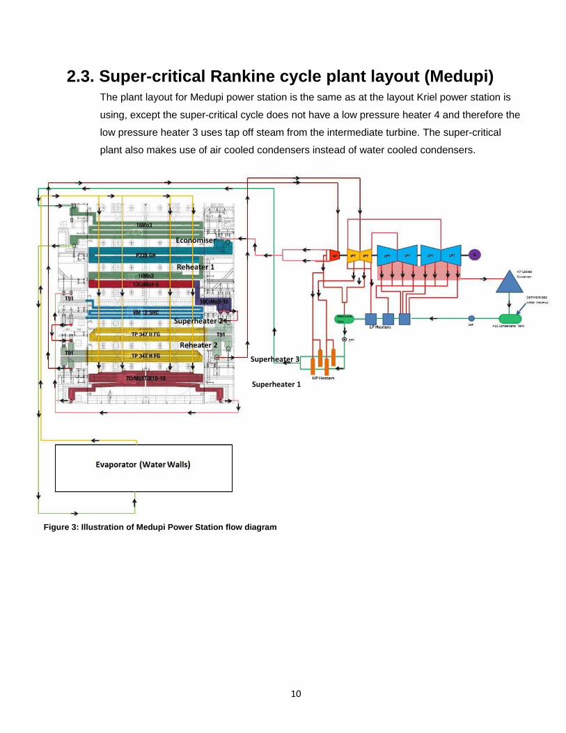
2.3. Super-critical Rankine cycle plant layout (Medupi) The plant layout for Medupi power station is the same as at the layout Kriel power station is
using, except the super-critical cycle does not have a low pressure heater 4 and therefore the
low pressure heater 3 uses tap off steam from the intermediate turbine. The super-critical
plant also makes use of air cooled condensers instead of water cooled condensers.
Economiser
Reheater 1
Reheater 2
Superheater 3
Superheater 1
Superheater 2
Figure 3: Illustration of Medupi Power Station flow diagram

11
2.4. Optimisation of Rankine cycle
2.4.1. Efficiency optimisation
To optimise the tap off pressure for the regenerative feed water heaters the pressure must be
decremented from the maximum tap off pressure to the minimum tap off pressure in a certain
number of intervals. Cycle efficiency is then plotted against the tap off pressure to get a trend
for the different points.
The picture below illustrates that the tap off steam at maximum is not allowed to expand
sufficiently in the turbine, therefore the efficiency is lower at maximum tap off pressure than at
lower tap off pressures (Harshal D Akolekar, 2014).
In the picture below it can also be concluded that steam lower than 1100 kPa is less efficient
to tap off. Because the energy in the steam is much lower at lower tap off pressures as it has
already lost a lot of energy in the turbine expansion, therefore much less energy can be
transferred to the boiler feed water.
Figure 4: Cycle efficiency plotted against feed heater tap off pressure (Harshal Akolekar, 2014)

12
2.4.2. Multi-objective optimisation
When optimising the Rankine cycle it is important not only to look at efficiency but at
mechanical work as well because mechanical work is also important as it will play a major role
in generating power. In figure 5 the extraction mass flow for the feed heaters is taken from
maximum to minimum mass flow. The efficiency is plotted on an x-y diagram (red line). The
net mechanical work is also plotted on an x-y2 scale (blue line). Because these two variables
have different scales it’s important to plot a local maximum/minimum line. The local
maximum/minimum line will indicate what the optimum point of these two variables is.
In figure 5 below it can be seen that the efficiency keeps improving as more mass flow is
taken, but this has a negative impact on the mechanical work as more energy is taken away
from the turbine and less turbine expansion takes place. That is why the net mechanical work
line reduces as more mass flow is tapped off.
This highlights the importance to use optimisation in the Rankine cycle
Figure 5: Cycle efficiency, net mechanical work and local minimum/maximum line plotted against steam extraction mass flow (Laure, 2011)
13
3. Development of the Rankine cycle and optimisation
3.1. Development of Rankine cycle For illustration purposes the following cycles were programed on EES using Kelvin for
temperature and kPa for pressure. Maximum pressure was taken as 16 000 kPa and minimum
as 5 kPa.
3.1.1. Carnot cycle
To illustrate the development of the Rankine cycle we will start at the Carnot cycle. Sadi
Carnot was the developer of the Carnot cycle and is applicable to any cycle such as steam
and gas.
Heat is added and rejected at constant temperatures. Compression and expansion are also
carried out at constant entropies. The Carnot is known as the ideal cycle as it offers maximum
efficiency between temperatures of source and sink.
Cycle efficiency can be represented by the net mechanical work output divided by the total
heat input.
Where and are the absolute temperatures of the source and sink (Rayaprolu, 2009).
In the illustration below (figure 6) on the T-s diagram the boiler produce steam at 16MPa and
condenses at 5kPa.
The Carnot cycle consists of four stages that are totally reversible.
The stages consist of:
Stage 1 – 2: Isothermal heat addition – Heat is supplied at constant temperature
Stage 2 – 3: Isentropic expansion – steam or gas expands from a high pressure and
temperature to a low pressure and temperature.
Stage 3 – 4: Isothermal heat rejection – Heat is rejected at constant temperature.
Stage 4 – 1: Isentropic compression – steam or gas is compressed from a low pressure and
temperature to a high pressure and temperature.
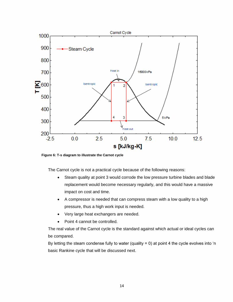
14
The Carnot cycle is not a practical cycle because of the following reasons:
Steam quality at point 3 would corrode the low pressure turbine blades and blade
replacement would become necessary regularly, and this would have a massive
impact on cost and time.
A compressor is needed that can compress steam with a low quality to a high
pressure, thus a high work input is needed.
Very large heat exchangers are needed.
Point 4 cannot be controlled.
The real value of the Carnot cycle is the standard against which actual or ideal cycles can
be compared.
By letting the steam condense fully to water (quality = 0) at point 4 the cycle evolves into ‘n
basic Rankine cycle that will be discussed next.
Figure 6: T-s diagram to illustrate the Carnot cycle

15
3.1.2. Basic Rankine cycle
The Rankine cycle is an idealised cycle for steam power plants and consists of the following
stages.
Figure 7: T-s diagram to illustrate the Basic Rankine cycle
Stages 5 - 1: Isobaric heat gain – Water enters the boiler under high pressure from the boiler
feed pump. Heat is added until the water reaches saturation point (1).
Stages 1 - 2: Isobaric heat gain – Further heat is added until the steam is fully saturated.
Stages 2 - 3: Isentropic expansion – The fully saturated steam expands in a turbine, producing
mechanical energy. Because of the expansion over the turbine blades the turbine rotates.
Stages 3 - 4: Isobaric heat rejection– The steam/water mixture enters the condenser where
the pressure is well below atmospheric pressure. The pressure and heat transfer forces the
mixture to reach the saturation point and become saturated water.
Stages 4 - 5: Isentropic compression – The boiler feed pump raises the pressure of the water.
Because the volume of saturated water is much smaller than saturated steam the work input
to raise the pressure is relatively small (THERMOPEDIA, 2011).
The steam quality at point 3 contains a lot of water content and is not ideal for the turbine
blades, as super heat is needed.

16
3.1.3. Rankine cycle with superheat
Figure 8: T-s diagram to illustrate the Rankine cycle with super heat
Stages 6 - 1: Isobaric heat gain – Water enters the boiler under high pressure from the boiler
feed pump. Heat is added until the water reaches saturation point (1).
Stages 1 - 2: Isobaric heat gain – Further heat is added until the steam is fully saturated.
Stages 2 - 3: Isobaric heat gain – Further heat is added until the steam reaches super steam.
This creates a higher steam temperature at constant pressure and more turbine expansion is
possible that creates more work output.
Stages 3 - 4: Isentropic expansion – The fully saturated steam expands in a turbine, producing
mechanical energy. Because of the expansion over the turbine blades the turbine rotates.
Stages 4 - 5: Isobaric heat rejection– The steam/water mixture enters the condenser where
the pressure is well below atmospheric pressure. The pressure and heat transfer force the
mixture to reach the saturation point and become saturated water.
Stages 5 - 6: Isentropic compression – The boiler feed pump raises the pressure of the water.
Because the volume of saturated water is much smaller than saturated steam and thus the
work input to raise the pressure is relatively small.
The steam quality at point 4 still contains a lot of water content and is not ideal for the turbine
blades, thus a reheat of the steam/water mixture is needed.

17
3.1.4. Rankine cycle with superheat and reheat
Figure 9: T-s diagram for the Rankine cycle with superheat and reheat
Stages 8 - 1: Isobaric heat gain – Water enters the boiler under high pressure from the boiler
feed pump. Heat is added until the water reaches saturation point (1).
Stages 1 - 2: Isobaric heat gain – Further heat is added until the steam is fully saturated.
Stages 2 - 3: Isobaric heat gain – Further heat is added until the steam reaches super-heated
steam. This creates a higher steam temperate at constant pressure and more turbine
expansion is possible that creates more work output.
Stages 3 - 4: Isentropic expansion – The fully saturated steam expands in a turbine, producing
mechanical energy. Because of the expansion over the turbine blades the turbine rotates.
Stages 4 - 5: Isobaric heat gain – The steam returns to the boiler and heat is added again to
reach super-heated steam. The steam is then returned to a second and third turbine for further
mechanical work.
Stages 5 - 6: Isentropic expansion – The steam expands in the second turbine before it fully
expands in the third turbine.
Stages 6 - 7: Isobaric heat rejection– The steam/water mixture enters the condenser where
the pressure is well below atmospheric pressure. The pressure and heat transfer force the
mixture to reach the saturation point to become saturated water.

18
Stages 6 - 7: Isentropic compression – The boiler feed pump raises the pressure of the water.
Because the volume of saturated water is much smaller than saturated steam the work input
to raise the pressure is relatively small.
The steam quality at point 6 contains very high steam content and can be used without
damaging the turbine blades.

19
3.1.5. Rankine cycle with superheat, reheat and feed water
heating
Figure 10: T-s diagram for the Rankine cycle with superheat, reheat and feed water heating
Feed water heating takes place to get a better efficiency. Looking at the Carnot cycle the
highest efficiency takes place if heat transfer takes place isothermally. Bled off steam from
various points on the turbines is used in this process (THERMOPEDIA, 2011).
Feed water heating takes place after the saturated water leaves the condenser. Low pressure
non-contact heaters use tap off steam from the second and third stage turbines to transfer
heat to the water before entering the de-aerator. The de-aerator is a contact heater which
uses tap off steam from the second stage turbine. The water is fed to the boiler feed pump
and then enters the high pressure non-contact heaters. Heat transfer takes place further in the
high pressure heaters before entering the boiler. High pressure heater one uses tap off steam
from the second stage turbine and high pressure heater two uses tap off steam from the cold
reheat line.
The stages remain the same as the previous illustration for the Rankine cycle with reheat. The
feed water heating transfers energy from the steam to the water, thus less energy is needed
from the coal, which results in a more effective overall Rankine cycle.

20
3.2. Steam quality at turbine outlet
3.2.1. Influence of boiler pressure
For this illustration the temperature and mass flow are held constant.
Figure 11 below illustrates a few different pressure lines on the T-s diagram and the effect of it
on the steam quality at the turbine exit.
Figure 11: T-s diagram with different pressure lines and the effect of it on the low pressure turbine outlet steam quality.
First we analyse the 16 MPa line (green line). The steam is heated to maximum temperature
(9), and then expands in the high pressure turbine (10) before it is reheated to maximum
temperature (11) again. The steam expands in the intermediate pressure turbine and then fully
in the low pressure turbine (12).
If the pressure is increased to 18 MPa (red line) a new pressure curve is visible. The same
process follows as above.
If the pressure is increased to 23 MPa (blue line) the pressure curve is above the two phase
stage, and this means that the super-critical stage is reached.

21
The steam quality at the low pressure turbine outlet decreases as the pressure increases (12
– 8 – 4), but the area under the graph increases, which means more net mechanical work.
With better metallurgical conditions the boiler pressure can be raised to increase the
mechanical work output.
3.2.2. Influence by maximum temperature
For this illustration the pressure and mass flow is held constant as well as the turbine
expansion pressure.
Figure 12 below illustrates a few different temperature lines on the T-s diagram and the effect
of it on the steam quality at the turbine exit
Figure 12: T-s diagram with different temperature lines and the effect of it on the low pressure turbine outlet steam quality.
First the lowest temperature is analysed (red line). The steam is heated to the maximum
temperature (1) before it expands in the high pressure turbine (2). The steam is heated again
to maximum temperature and then expands in the intermediate and low pressure turbines (4).
Figure 12 above illustrates the rising of the maximum temperature to point 5 (blue line) and
also point 9 (yellow line). The same process as above follows.

22
The illustration shows that if the temperature increases the steam quality at the low pressure
turbine outlet increases. This is ideal for the low pressure turbine blades.
3.2.3. Influence by high pressure turbine expansion
For this illustration the temperature, mass flow and boiler pressure are held constant.
Figure 13 below illustrates a few different pressure lines on the T-s diagram and the effect of
the high pressure turbine expansion on the steam quality at the turbine exit.
Figure 13: T-s diagram to illustrate the high pressure turbine expansion and the effect of it on the low pressure turbine outlet steam quality
If the high pressure turbine expands further to point 5, then the pressure line changes
because the turbine expands further and more work is done, therefore more energy is used.
Thus the steam should gain more heat in the reheater than previously. With the lower
pressure line because of further expansion the steam quality improves at the low pressure
turbine outlet (6).
The area under the graph increases, thus net mechanical work increases. The high pressure
turbine expansion is restricted by the capability of the heat gain in the reheater as well as the
low pressure turbine outlet steam quality.

23
3.3. Natural vs forced circulation boilers
3.3.1. Natural circulation (steam drum boilers)
Natural circulation boilers use a steam drum. The steam drum level is maintained by the boiler
feed pump. The water is fed into the steam drum and travels down to the bottom mud drum
where it is fed into the boiler tubes. Heat is applied and the hot water rises to the top where it
accumulates and enters the drum again. The drum separates the steam and the water where
the water goes down to the bottom mud drum again. The steam travels to the superheater for
further heating. The steam drum has a fixed separation point, which means a molecule of
water can make many passes through the evaporation tubes before turning into steam for
further heating.
Figure 14: Illustration of the flow for drum boilers (Power)
Advantages
Easier construction and cheaper to build, no spiral wall required.
Less water consumption.
More tolerant of feed water impurities.
High reliability.
Constant heat transfer areas.
High partial load range.
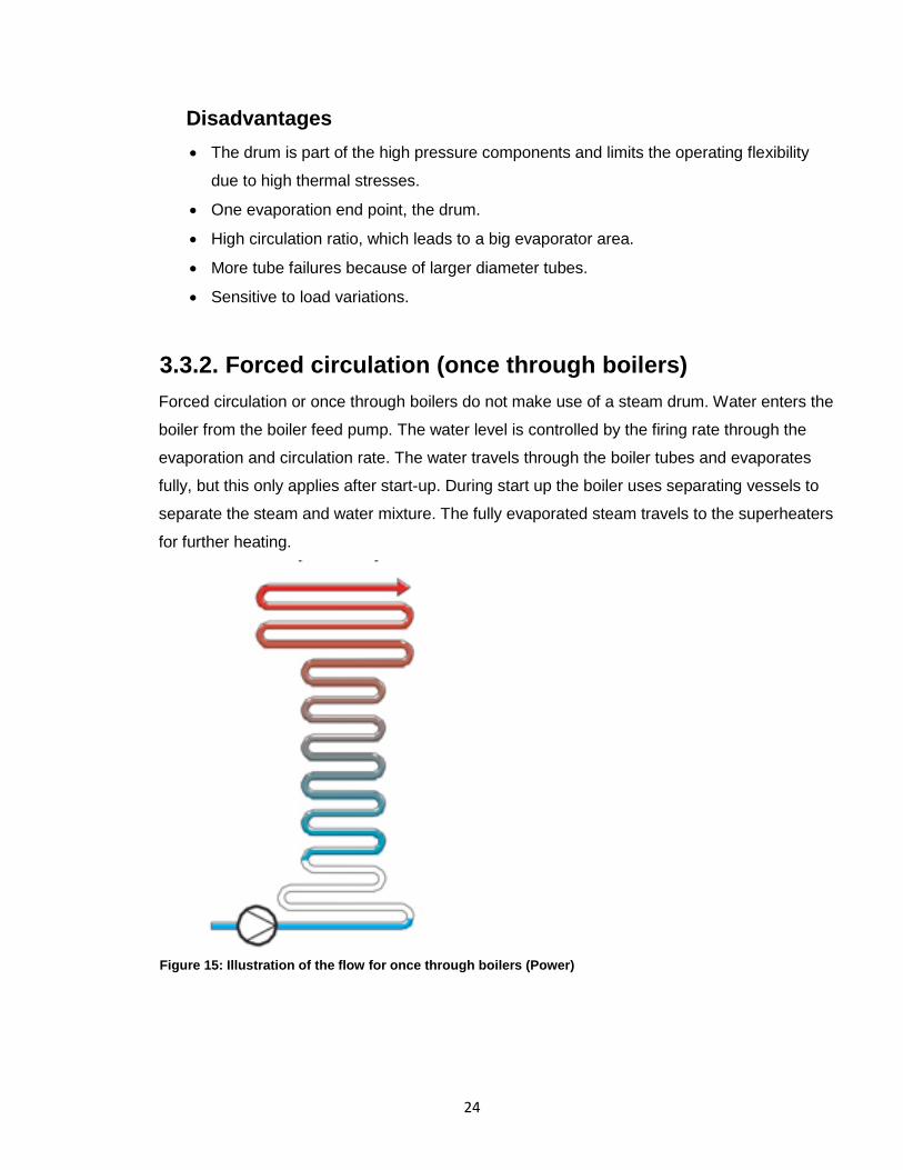
24
Disadvantages
The drum is part of the high pressure components and limits the operating flexibility
due to high thermal stresses.
One evaporation end point, the drum.
High circulation ratio, which leads to a big evaporator area.
More tube failures because of larger diameter tubes.
Sensitive to load variations.
3.3.2. Forced circulation (once through boilers)
Forced circulation or once through boilers do not make use of a steam drum. Water enters the
boiler from the boiler feed pump. The water level is controlled by the firing rate through the
evaporation and circulation rate. The water travels through the boiler tubes and evaporates
fully, but this only applies after start-up. During start up the boiler uses separating vessels to
separate the steam and water mixture. The fully evaporated steam travels to the superheaters
for further heating.
Figure 15: Illustration of the flow for once through boilers (Power)

25
Advantages
Does not have a high pressure drum, thus more operating flexibility and lower stress
operation.
High overall efficiency, even at part loads.
Shorter start-up time.
Suitable for all coal grades.
More equal distribution of the water in the tubes.
Ideal for sliding pressure operation, thus more control over load changes.
Produces less CO2, because it is more efficient.
Disadvantages
It’s necessary for higher grade material as the evaporator forms part of the first
superheater.
Difficult construction because of spiral tubes.
Feed pump needed for forced circulation.
Higher water consumption.
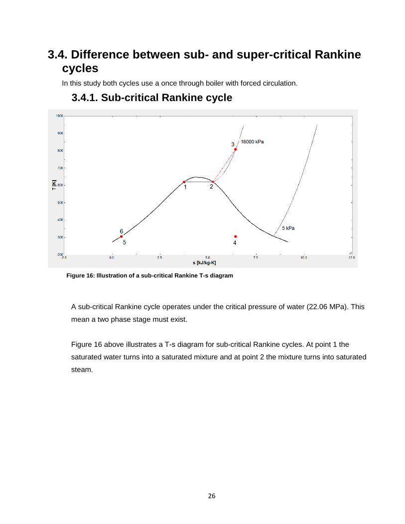
26
3.4. Difference between sub- and super-critical Rankine cycles In this study both cycles use a once through boiler with forced circulation.
3.4.1. Sub-critical Rankine cycle
Figure 16: Illustration of a sub-critical Rankine T-s diagram
A sub-critical Rankine cycle operates under the critical pressure of water (22.06 MPa). This
mean a two phase stage must exist.
Figure 16 above illustrates a T-s diagram for sub-critical Rankine cycles. At point 1 the
saturated water turns into a saturated mixture and at point 2 the mixture turns into saturated
steam.

27
3.4.2. Super-critical Rankine cycle
A
Super-critical Rankine cycle operates above the critical pressure of water (22.06 MPa). This
mean no two phase stage exists.
Figure 17 illustrates the T-s diagram for super-critical cycles. Point 4 is the critical point for this
cycle where water transfers into steam without a two stage phase.
With better metallurgical conditions higher pressure and temperature can be achieved,
therefore super-critical cycles are possible. With the possibility to increase the pressure and
temperature a higher efficiency and net mechanical work can be reached.
Figure 17: Illustration of a super-critical Rankine cycle T-s diagram

28
4. Rankine cycle programming methodology to enable optimisation
4.1. Rankine cycle efficiency
4.1.1. Increasing boiler pressure
One way to increase the Rankine cycle efficiency is to increase the boiler pressure at constant
temperature. This will increase the pressure where evaporation takes places.
By using the Rankine cycle efficiency formula the following can be concluded
From figure 18 a slight increase in heat in ( ) and work in ( ), with a significantly increase
in work out ( ) can be observed, therefore increases.
The area represented the increase in net mechanical work is greater that the area that
represents a decrease in net mechanical work (B-Cubed, 2014)
Figure 18: Effect of boiler pressure on net mechanical work (Laure, 2011)
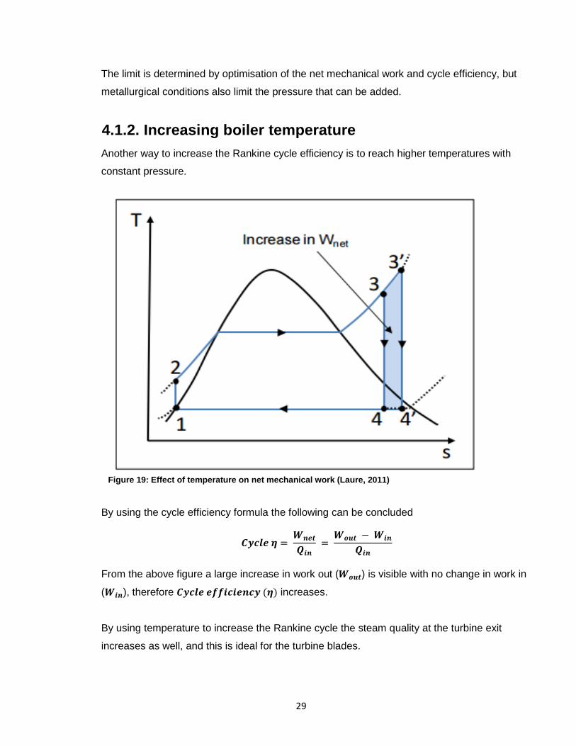
29
The limit is determined by optimisation of the net mechanical work and cycle efficiency, but
metallurgical conditions also limit the pressure that can be added.
4.1.2. Increasing boiler temperature
Another way to increase the Rankine cycle efficiency is to reach higher temperatures with
constant pressure.
By using the cycle efficiency formula the following can be concluded
From the above figure a large increase in work out ( ) is visible with no change in work in
( ), therefore increases.
By using temperature to increase the Rankine cycle the steam quality at the turbine exit
increases as well, and this is ideal for the turbine blades.
Figure 19: Effect of temperature on net mechanical work (Laure, 2011)

30
The incensement of temperature is limited by metallurgical conditions and economical
infrastructure as the heat added will also be increased (Electrical4u.com, 2015).
4.1.3. Lowering the condenser pressure
By lowering the condenser pressure an increase in the Rankine cycle efficiency is possible.
This way more turbine expansion is possible.
By using the cycle efficiency formula the following can be concluded
From the above figure 20 work out ( ) increases significantly while work in ( ) increases
slightly, therefore will also increase.
The limit for condenser pressure is limited by cooling water temperature, which will influence
the saturation pressure of the mixture entering the condenser. Steam quality at the turbine exit
will increase as the condenser pressure decrease. This is not ideal for the turbine blades
(Electrical4u.com, 2015).
Figure 20: Effect of lowering the condenser pressure on net mechanical work (Laure, 2011)

31
5. Programming of sub- and supercritical Rankine cycles
Both cycles are based on once through boilers and drum boilers were not taken in account.
5.1. Sub-critical Rankine cycle This cycle was programmed in EES by using the heat balance diagram of Kriel power station at
maximum output (500 MW).
5.1.1. Rankine cycle without optimisation
5.1.1.1. Condenser outlet
The condenser outlet temperature is held constant by ignoring the ambient temperature,
and this serves as the first variable. The condenser is a heat exchanger and extracts heat
from the steam/water mixture, therefore saturated water can be expected at the
condenser outlet. With two known variables the rest can be calculated.
5.1.1.2. Extraction pump discharge
The extraction pump has a constant pressure because the de-aerator has a regulating
valve between the extraction pump and de-aerator inlet. With the pressure constant the
first variable is known. Because the extraction pump uses saturated water coming from
the condenser outlet the second variable is known.
But because the extraction pump has efficiency the following equation should apply.

32
With this equation can be calculated for the extraction pump.
With these variables known the rest can be calculated.
Figure 21: Enthalpy plotted against Entropy to illustrate the effect of efficiency of a pump (An analysis of a thermal power plant working on a Rankine cycle: A theoretical investigation, 2008)
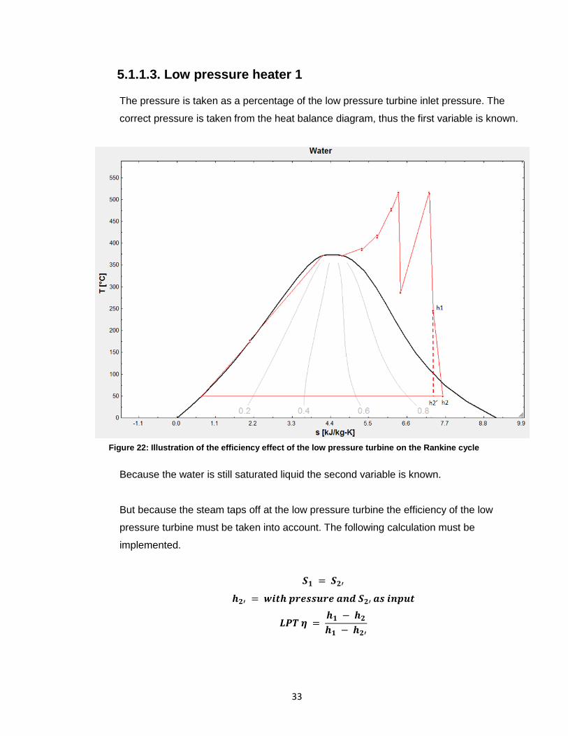
33
5.1.1.3. Low pressure heater 1
The pressure is taken as a percentage of the low pressure turbine inlet pressure. The
correct pressure is taken from the heat balance diagram, thus the first variable is known.
Because the water is still saturated liquid the second variable is known.
But because the steam taps off at the low pressure turbine the efficiency of the low
pressure turbine must be taken into account. The following calculation must be
implemented.
Figure 22: Illustration of the efficiency effect of the low pressure turbine on the Rankine cycle

34
With this equation can be calculated for the pressure of low pressure heater 1. With
these variables the rest can be calculated.
5.1.1.4. Low pressure heater 2
The pressure is taken as a percentage of the low pressure turbine inlet pressure. The
correct pressure is taken from the heat balance diagram, thus the first variable is known.
Because the water is still saturated liquid the second variable is known.
The same calculation for low pressure heater 1 (5.1.1.3) applies for low pressure heater 2
to compensate for the efficiency effect. With these variables the rest can be calculated.
5.1.1.5. Low pressure heater 3
The pressure is taken as a percentage of the low pressure turbine inlet pressure. The
correct pressure is taken from the heat balance diagram, thus the first variable is known.
Because the water is still saturated liquid the second variable is known.
The same calculation for low pressure heater 1 (5.1.1.3) applies for low pressure heater 3
to compensate for the efficiency effect. With these variables the rest can be calculated.
5.1.1.6. Low pressure heater 4
The pressure is taken as a percentage of the intermediate pressure turbine inlet pressure.
The correct pressure is taken from the heat balance diagram, thus the first variable is
known. Because the water is still saturated liquid the second variable is known.
But because the steam taps off at the intermediate pressure turbine the efficiency of the
intermediate pressure turbine must be taken into account. The following calculation must
be implemented.

35
With this equation can be calculated for the pressure of low pressure heater 4.
5.1.1.7. De-aerator
The pressure is taken as a percentage of the intermediate pressure turbine inlet pressure.
The correct pressure is taken from the heat balance diagram, thus the first variable is
known. Because the water is still saturated liquid the second variable is known.
The same calculation for low pressure heater 4 (5.1.1.6) applies for the de-aerator to
compensate for the efficiency effect. With these variables the rest can be calculated.
Figure 23: Illustration of the efficiency effect of the intermediate pressure turbine on the Rankine cycle

36
5.1.1.8. High pressure heater 6
The pressure is taken as a percentage of the intermediate pressure turbine inlet pressure.
The correct pressure is taken from the heat balance diagram, thus the first variable is
known. Because the water is still saturated liquid the second variable is known.
The same calculation for low pressure heater 4 (5.1.1.6) applies for high pressure heater
6 to compensate for the efficiency effect. With these variables known the rest can be
calculated.
5.1.1.9. High pressure heater 7
Because high pressure heater 7 taps steam off from the high pressure turbine outlet line
(cold reheat line) the pressure cannot differ too much. A percentage of 0.1 is taken for the
pressure loss in the cold reheat line. With the pressure known and the water is still liquid
two variables are known.
The same calculation for low pressure heater 4 (5.1.1.6) applies for high pressure heater
7 to compensate for the efficiency effect. With these variables the rest can be calculated.
5.1.1.10. Boiler feed pump
The maximum pressure is known and the water is still saturated liquid, thus two variables
are known. With two known variables the rest of the variables can be calculated.
But because the boiler feed pump has an efficiency the following equation should apply.

37
Figure 24: Enthalpy plotted against Entropy to illustrate the effect of efficiency on a pump (An analysis of a thermal power plant working on a Rankine cycle: A theoretical investigation, 2008)
With this equation can be calculated for the pressure output of the boiler feed pump
pressure. With these variables known the rest can be calculated.
5.1.1.11. Evaporator
The pressure is taken as a percentage of the maximum pressure to compensate for the
pressure loss in the lines and evaporator tubes.
A procedure was programmed to determine whether the pressure is sub-critical or super-
critical. If the pressure is sub-critical a two-phase mixture should exist and the water turns
from saturated liquid to saturated steam. Thus two variables are known and the rest can
be calculated.
If the pressure is super-critical the pressure line missed the two phase stage and the
critical point for water is reached. Thus two variables are known and the rest can be
calculated.

38
5.1.1.12. Superheater attemperator 1
5.1.1.12.1. Inlet
The pressure is taken as a percentage of the evaporator inlet pressure to compensate
for the pressure loss in the main steam pipes.
The temperature is taken as a percentage loss in in the main steam pipelines.
5.1.1.12.2. Outlet
The temperature that is tempered off is taken from the heat balance diagram and as a
percentage of the maximum temperature. The entropy is kept the same as the inlet.
With two variables known the rest can be calculated.
5.1.1.13. Superheaters
5.1.1.13.1. Superheater 1
The temperature and pressure for superheater 1 inlet are the same as attemperator 1
outlet, because attemperator 1 is situated at the superheater 1 inlet. The outlet
pressure and temperature are taken from the heat balance diagram and are a
percentage of the maximum temperature.
5.1.1.14. Superheater attemperator 2
5.1.1.14.1. Inlet
The pressure is taken as a percentage of the superheater 1 inlet pressure to
compensate for the pressure loss in superheater 1 tubes.
The temperature is taken as a percentage of the maximum temperature to
compensate for the temperature gain in superheater 1.

39
5.1.1.14.2. Outlet
The temperature that is tempered off is taken from the heat balance diagram and is
taken as a percentage of the maximum temperature. The entropy is kept the same as
the inlet.
With two variables known the rest can be calculated.
5.1.1.15. Superheater 2
The temperature and pressure for superheater 2 are the same as the attemperator 2
outlet, because attemperator 2 is situated at the superheater 2 inlet. The outlet
pressure and temperature are taken from the heat balance diagram and are a
percentage of the maximum temperature.
5.1.1.16. Superheater attemperator 3
5.1.1.16.1. Inlet
The pressure is taken as a percentage of the superheater 2 inlet pressure to
compensate for the pressure loss in superheater 2 tubes.
The temperature is taken as a percentage of the maximum temperature to
compensate for the temperature gain in superheater 2.
5.1.1.16.2. Outlet
The temperature that is tempered off is taken from the heat balance diagram and is
taken as a percentage of the maximum temperature. The entropy is kept the same as
the inlet.
With two variables known the rest can be calculated.
5.1.1.17. Superheater 3
The temperature and pressure for superheater 3 is the same as attemperator 3 outlet,
because attemperator 3 is situated at superheater 3 inlet. The outlet pressure and

40
temperature are taken from the heat balance diagram and are a percentage of the
maximum temperature.
With two variables known the rest can be calculated.
5.1.1.18. High pressure turbine
5.1.1.18.1. Inlet
The pressure is taken as a percentage of superheater 3 inlet pressure. The
temperature is taken as the maximum temperature.
With two variables known the rest can be calculated.
5.1.1.18.2. Outlet
The pressure is taken as a percentage of the inlet pressure.
Because the high pressure turbine has an efficiency the following equation should
apply.
Figure 25: Illustration of the efficiency effect of the intermediate pressure turbine on the Rankine cycle

41
With this equation can be calculated for the pressure output of the high pressure
turbine.
With two variables known the rest can be calculated.
5.1.1.19. Reheater attemperators
5.1.1.19.1. Inlet
The pressure is taken as a percentage of high pressure turbine outlet pressure and the
pressure loss to high pressure heater 7. The temperature is taken to be the same as
the high pressure turbine outlet.
With two variables known the rest can be calculated.
5.1.1.19.2. Outlet
The temperature that is tempered off is taken from the heat balance diagram and is
taken as a percentage of the maximum temperature. The entropy is kept the same as
the inlet.
With two variables known the rest can be calculated.
5.1.1.20. Reheaters
The pressure is taken as a percentage of the attemperators outlet pressure. The
temperature is taken as the maximum temperature.
With two variables known the rest can be calculated.

42
5.1.1.21. Intermediate pressure turbine
The pressure is taken as a percentage of the Reheater outlet pressure to compensate for
the pressure loss in hot reheat line.
Because the intermediate pressure turbine has an efficiency the following equation should
apply.
With this equation can be calculated for the pressure output of the intermediate
pressure turbine.
With two variables known the rest can be calculated.
Figure 26: Illustration of the efficiency effect of the intermediate pressure turbine on the Rankine cycle

43
5.1.1.22. Low pressure turbine
The pressure is taken as a percentage of the low pressure turbine to compensate for the
pressure loss through the intermediate turbine.
Because the low pressure turbine has an efficiency the following equation should apply.
With this equation can be calculated for the pressure output of the low pressure
turbine.
With two variables known the rest can be calculated.
Figure 27: Illustration of the efficiency effect of the low pressure turbine on the Rankine cycle
44
5.1.1.23. Superheater attemperators tap off point
The pressure for the tap off point for the superheaters is taken as the maximum pressure.
The enthalpy is taken as the feed pump outlet enthalpy.
With two variables known the rest can be calculated.
5.1.1.24. Reheater attemperators tap off point
The pressure for the tap off point for the Reheaters is taken as a percentage of the
maximum pressure because the tap off point is on the interconnecting stage of the feed
pump. The enthalpy is taken on the same line as the feed pump with the corresponding
pressure.
5.1.2. Optimisation of the sub-critical Rankine cycle
5.1.2.1. Boiler feed pump
A factor line was programmed to get the optimal for both efficiency and net mechanical
work. The following equation was used.
The factor line is divided by a number to fit in on the scale with the cycle efficiency.
A new parametric table was created with 500 runs. The boiler feed pump was run from 5
MPa to 48 MPa in even distributing increments. The net mechanical work, cycle efficiency
and the factor line are used as variables of the pressure.
The results is plotted on a graph to get the optimal point
5.1.2.2. High pressure turbine expansion pressure
A new parametric table was created with 500 runs. The high pressure turbine expansion
pressure was run from 10% to 90% of the expansion pressure. The pressure, net
mechanical work, cycle efficiency and the factor line were added as variables.
The results is plotted on a graph to get the optimal point

45
The optimal point is limited by the steam quality at the low pressure turbine outlet. In this
study we did not want to compromise the low pressure turbine blades and kept the steam
quality as designed.
5.1.2.3. High pressure heater 6 tap off pressure
A new parametric table was created with 500 runs. The tap off pressure was taken as a
percentage of the intermediate turbine inlet pressure. The tap off pressure percentage
was run from 0.01% to 99.99%. The pressure, net mechanical work, cycle efficiency and
the factor line were added as variables.
The results are plotted on a graph to get the optimal point
An assumption is made that a minimum pressure loss of 33% through the Intermediate
pressure turbine was possible.
5.1.2.4. De-aerator tap off pressure
A new parametric table was created with 500 runs. The tap off pressure was taken as a
percentage of the intermediate turbine inlet pressure. The tap off pressure percentage
was run from 0.01% to 99.99%. The pressure, net mechanical work, cycle efficiency and
the factor line were added as variables.
The results are plotted on a graph to get the optimal point. An assumption is made that a
minimum pressure loss of 33% through the Intermediate pressure turbine was possible.
5.1.2.5. Low pressure heater 4 tap off pressure
A new parametric table was created with 500 runs. The tap off pressure was taken as a
percentage of the intermediate turbine inlet pressure. The tap off pressure percentage
was run from 0.01% to 99.99%. The pressure, net mechanical work, cycle efficiency and
the factor line were added as variables.
The results are plotted on a graph to get the optimal point
The minimum pressure that can be achieved for the tap off point is equal to the
intermediate pressure turbine outlet pressure.
46
5.1.2.6. Low pressure heater 3 tap off pressure
A new parametric table was created with 500 runs. The tap off pressure was taken as a
percentage of the low pressure turbine inlet pressure. The tap off pressure percentage
was run from 0.01% to 99.99%. The pressure, net mechanical work, cycle efficiency and
the factor line were added as variables.
The results are plotted on a graph to get the optimal point.
An assumption is made that a minimum pressure loss of 33% through the low pressure
turbine is possible.
5.1.2.7. Low pressure heater 2 tap off pressure
A new parametric table was created with 500 runs. The tap off pressure was taken as a
percentage of the low pressure turbine inlet pressure. The tap off pressure percentage
was run from 0.01% to 99.99%. The pressure, net mechanical work, cycle efficiency and
the factor line were added as variables.
The results are plotted on a graph to get the optimal point.
No change was visible to the net mechanical work or efficiency for different pressures.
5.1.2.8. Low pressure heater 1 tap off pressure
A new parametric table was created with 500 runs. The tap off pressure was taken as a
percentage of the low pressure turbine inlet pressure. The tap off pressure percentage
was run from 0.01% to 99.99%. The pressure, net mechanical work, cycle efficiency and
the factor line were added as variables.
The results are plotted on a graph to get the optimal point
No change visible to the net mechanical work or efficiency for different pressures.

47
5.2. Super-critical Rankine cycle This cycle was programmed in EES by using the heat balance diagram of Medupi power
station at maximum output (794 MW).
5.2.1. Rankine cycle without optimisation
The same programming method used in 5.1 applies for the super-critical cycle except the
cycle does not have a low pressure heater 4, therefore the only difference is the low pressure
heater 3 steam tap off point is situated on the Intermediate pressure turbine instead of the low
pressure turbine as in the above sub-critical cycle. Only the new tap off point will be discussed
for the super-critical cycle.
The pressure is taken as a percentage of the intermediate pressure turbine inlet pressure. The
correct pressure is taken from the heat balance diagram, thus the first variable is known.
Because the water is still saturated liquid the second variable is known and the rest of the
variables can be calculated.
But because the steam taps off at the intermediate pressure turbine the efficiency of the
intermediate pressure turbine must be taken into account. The following calculation must be
implemented.
Figure 28: Illustration of the efficiency effect of the intermediate pressure turbine on the Rankine cycle

48
With this equation can be calculated for the pressure of low pressure heater 3.
5.3. Sub- and super-critical Rankine cycle optimisation Two optimisation methods are used to determine whether the order of optimisation makes a
difference.
5.3.1. Optimisation method 1
This method was based on the following steam tap off order.
Feed pump – High pressure turbine expansion pressure – High pressure heater 6 – De-
aerator – Low pressure heater 4 (only applies for sub-critical cycle) – Low pressure heater 3 -
Low pressure heater 2 - Low pressure heater 1.
Then the cycle repeats itself for the second and third runs. After the third run the boiler feed
pump pressure and high pressure expansion pressure were optimised to see whether any
values differed.
After the third run the values became stable and there was no need for any further runs.
The optimisation method is the same for super-critical cycle except low pressure heater 4
does not exist.
5.3.2. Optimisation method 2
This method was based on the following steam tap off order.
Feed pump – High pressure heater 6 – High pressure turbine expansion pressure – Low
pressure heater 1 – Low pressure heater 2 - Low pressure heater 3 - Low pressure heater 4
(only applies for sub-critical cycle).

49
Then the cycle repeats for the second and third run. After the third run the boiler feed pump
pressure and high pressure expansion pressure was optimised to see if any values differ.
After the third run the values become stable and there was no need for any further runs.
The optimisation method is the same for super-critical cycle except low pressure heater 4
doesn’t exist.

50
6. Results of sub- and super-critical Rankine cycles
6.1. Sub-critical optimisation results The sub critical cycle was based on the heat balance diagrams for Kriel power station at 500MW
(full load) output.
6.1.1. Sub-critical cycle without optimisation
6.1.1.1. Input parameters
The input parameters are taken from the original heat balance diagram for Kriel power
station.
Table 1: Sub-critical boiler input parameters as on the heat balance diagram
6.1.1.2. Results
Feed pump 22.15 MPa
Maximum Temperature 516°C
Minimum Temperature 40°C
Maximum mass flow 415 kg/s
Extraction pump discharge pressure 2.388 MPa
High pressure heater 6 bled steam tap off pressure 1.738 MPa
De-aerator bled steam tap off pressure 1.032 MPa
Low pressure heater 4 bled steam tap off pressure 0.4106 MPa
Low pressure heater 3 bled steam tap off pressure 0.1743 MPa
Low pressure heater 2 bled steam tap off pressure 0.06046 MPa
Low pressure heater 1 bled steam tap off pressure 0.02991 MPa
Cycle efficiency 42.69 %
Mega Watt out 538.4 MW
Total Work in 28.68 kJ
Total Work Out 1326 kJ
Net mechanical work 1297 kJ
Heat added 3039 kJ
Heat rejected 1553 kJ
Table 2: Results for sub-critical cycle from input parameters before optimisation

51
Figure 29: T-s diagram after programmed on EES for sub-critical cycle before any optimisation
Figure 30: Illustration of Kriel power station plant layout

52
6.1.2. Sub-critical cycle optimisation – first method
6.1.2.1. First run
6.1.2.1.1. Boiler feed pump pressure
Figure 32: Cycle efficiency, net mechanical work and the factor line plotted against boiler feed pump discharge pressure (1st method, 1st run)
Figure 31: Cycle efficiency, net-work and the factor line plotted against boiler feed pump discharge pressure (Zoomed in) (1st method, 1st run)

53
6.1.2.1.2. High pressure turbine expansion
Figure 33: Cycle efficiency, net mechanical work and the factor line plotted against the high pressure turbine expansion pressure (1st method, 1st run)
Before optimisation
After optimisation
High pressure turbine expansion pressure
3.715 MPa
High pressure turbine expansion pressure
3.151 MPa
Cycle efficiency 42.92%
Cycle efficiency 42.88%
Mega Watt output 535.6 MW
Mega Watt output 547.5 MW
Net mechanical work 1291 kJ
Net mechanical work 1319 kJ
Heat added 3007 kJ
Heat added 3077 kJ
Heat rejected 1525 kJ
Heat rejected 1575 kJ
LPT outlet steam quality 0.9196 LPT outlet steam quality 0.9288 Table 4: Before and after optimisation results for the high pressure turbine expansion pressure (1st method, 1st run)
Before optimisation
After optimisation
Boiler feed pump pressure 22.14 MPa
Boiler feed pump pressure 24.3 MPa
Cycle efficiency 42.69%
Cycle efficiency 42.92%
Mega Watt output 538.4 MW
Mega Watt output 535.6 MW
Net mechanical work 1397 kJ
Net mechanical work 1291 kJ
Heat added 3039 kJ
Heat added 3007 kJ
Heat rejected 1553 kJ
Heat rejected 1525 kJ
Table 3: Before and after optimisation results for the boiler feed pump pressure (1st method, 1st run)
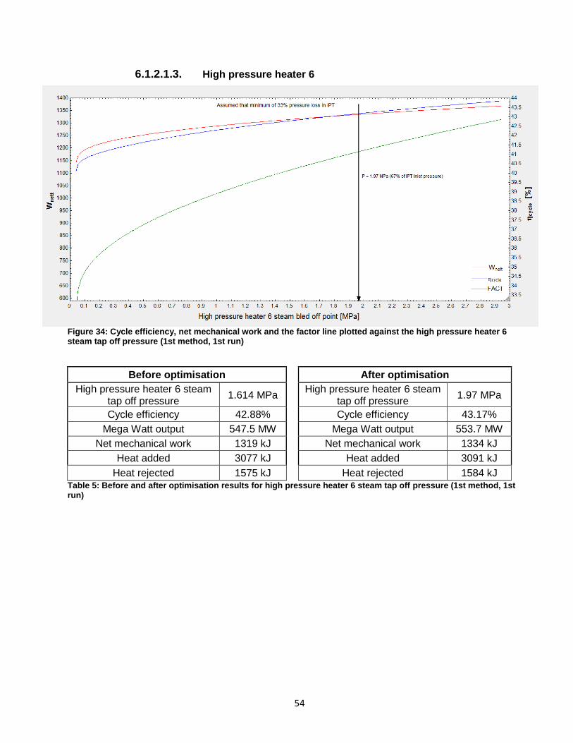
54
6.1.2.1.3. High pressure heater 6
Figure 34: Cycle efficiency, net mechanical work and the factor line plotted against the high pressure heater 6 steam tap off pressure (1st method, 1st run)
Before optimisation
After optimisation
High pressure heater 6 steam tap off pressure
1.614 MPa
High pressure heater 6 steam tap off pressure
1.97 MPa
Cycle efficiency 42.88%
Cycle efficiency 43.17%
Mega Watt output 547.5 MW
Mega Watt output 553.7 MW
Net mechanical work 1319 kJ
Net mechanical work 1334 kJ
Heat added 3077 kJ
Heat added 3091 kJ
Heat rejected 1575 kJ
Heat rejected 1584 kJ Table 5: Before and after optimisation results for high pressure heater 6 steam tap off pressure (1st method, 1st run)

55
6.1.2.1.4. De-aerator
Figure 35: Cycle efficiency, net mechanical work and the factor line plotted against the de-aerator steam bled off pressure (1st method, 1st run)
Before optimisation
After optimisation
High pressure heater 6 steam tap off pressure
0.9581 MPa
High pressure heater 6 steam tap off pressure
1.97 MPa
Cycle efficiency 43.17%
Cycle efficiency 45.43%
Mega Watt output 553.7 MW
Mega Watt output 554.3 MW
Net mechanical work 1334 kJ
Net mechanical work 1336 kJ
Heat added 3091 kJ
Heat added 2940 kJ
Heat rejected 1584 kJ
Heat rejected 1589 kJ Table 6: Before and after optimisation results for the De-aerator steam tap off pressure (1st method, 1st run)

56
6.1.2.1.5. Low pressure heater 4
Figure 36: Cycle efficiency, net mechanical work and the factor line plotted against low pressure heater 4 steam bled off pressure (1st method, 1st run)
Before optimisation
After optimisation
Low pressure heater 4 steam tap off pressure
0.3812 MPa
Low pressure heater 4 steam tap off pressure
0.3791 MPa
Cycle efficiency 45.43%
Cycle efficiency 45.43%
Mega Watt output 554.3 MW
Mega Watt output 554.3 MW
Net mechanical work 1336 kJ
Net mechanical work 1336 kJ
Heat added 2940 kJ
Heat added 2940 kJ
Heat rejected 1589 kJ
Heat rejected 1589 kJ Table 7: Before and after optimisation results for low pressure heater 4 steam tap off pressure (1st method, 1st run)

57
6.1.2.1.6. Low pressure heater 3
Figure 37: Cycle efficiency, net mechanical work and the factor line plotted against low pressure heater 3 steam bled off pressure (1st method, 1st run)
Before optimisation
After optimisation
Low pressure heater 3 steam tap off pressure
0.1618 MPa
Low pressure heater 3 steam tap off pressure
0.2548 MPa
Cycle efficiency 45.43%
Cycle efficiency 45.86%
Mega Watt output 554.3 MW
Mega Watt output 559.6 MW
Net mechanical work 1336 kJ
Net mechanical work 1348 kJ
Heat added 2940 kJ
Heat added 2940 kJ
Heat rejected 1589 kJ
Heat rejected 1591 kJ Table 8: Before and after optimisation results for low pressure heater 3 steam tap off pressure (1st method, 1st run)

58
6.1.2.1.7. Low pressure heater 2
Figure 38: Cycle efficiency, net mechanical work and the factor line plotted against low pressure heater 2 steam bled off pressure (1st method, 1st run)
Before optimisation
After optimisation
Low pressure heater 2 steam tap off pressure
0.05614 MPa
Low pressure heater 2 steam tap off pressure
0.05614 MPa
Cycle efficiency 45.86%
Cycle efficiency 45.86%
Mega Watt output 559.6 MW
Mega Watt output 559.6 MW
Net mechanical work 1348 kJ
Net mechanical work 1348 kJ
Heat added 2940 kJ
Heat added 2940 kJ
Heat rejected 1591 kJ
Heat rejected 1591 kJ Table 9: Before and after optimisation results for low pressure heater 2 steam tap off pressure (1st method, 1st run)

59
6.1.2.1.8. Low pressure heater 1
Figure 39: Cycle efficiency, net mechanical work and the factor line plotted against low pressure heater 1 steam bled off pressure (1st method, 1st run)
Before optimisation
After optimisation
Low pressure heater 1 steam tap off pressure
0.05614 MPa
Low pressure heater 1 steam tap off pressure
0.05614 MPa
Cycle efficiency 45.86%
Cycle efficiency 45.86%
Mega Watt output 559.6 MW
Mega Watt output 559.6 MW
Net mechanical work 1348 kJ
Net mechanical work 1348 kJ
Heat added 2940 kJ
Heat added 2940 kJ
Heat rejected 1591 kJ
Heat rejected 1591 kJ Table 10: Before and after optimisation results for low pressure heater 4 steam tap off pressure (1st method, 1st run)
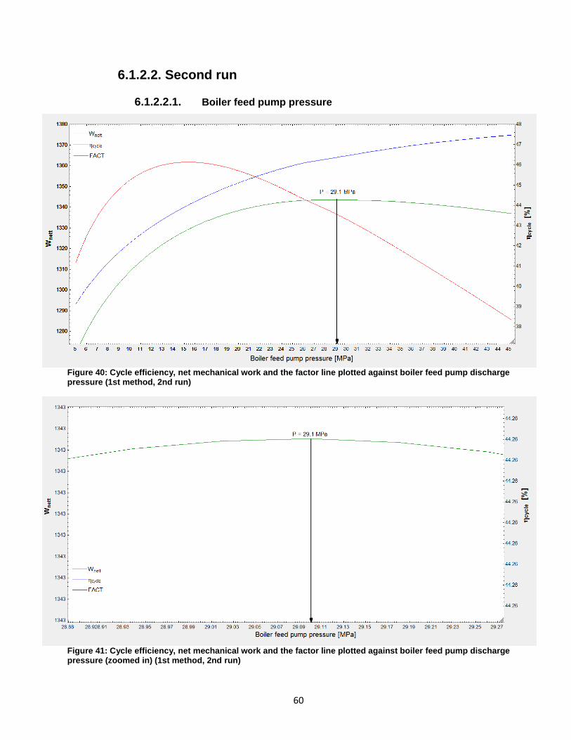
60
6.1.2.2. Second run
6.1.2.2.1. Boiler feed pump pressure
Figure 40: Cycle efficiency, net mechanical work and the factor line plotted against boiler feed pump discharge pressure (1st method, 2nd run)
Figure 41: Cycle efficiency, net mechanical work and the factor line plotted against boiler feed pump discharge pressure (zoomed in) (1st method, 2nd run)

61
Before optimisation
After optimisation
Boiler feed pump pressure 24.3 MPa
Boiler feed pump pressure 29.1 MPa
Cycle efficiency 45.86%
Cycle efficiency 46.37%
Mega Watt output 559.6 MW
Mega Watt output 554.6 MW
Net mechanical work 1348 kJ
Net mechanical work 1336 kJ
Heat added 2940 kJ
Heat added 2882 kJ
Heat rejected 1591 kJ
Heat rejected 1550 kJ Table 11: Before and after optimisation results for the boiler feed pump discharge pressure (1
st method, 2
nd run)
6.1.2.2.2. High pressure turbine expansion
Figure 42: Cycle efficiency, net mechanical work and the factor line plotted against the high pressure turbine expansion pressure (1st method, 2nd run)
Before optimisation
After optimisation
High pressure turbine expansion pressure
3.618 MPa
High pressure turbine expansion pressure
3.149 MPa
Cycle efficiency 46.37%
Cycle efficiency 46.09%
Mega Watt output 554.6 MW
Mega Watt output 563.5 MW
Net mechanical work 1336 kJ
Net mechanical work 1358 kJ
Heat added 2882 kJ
Heat added 2946 kJ
Heat rejected 1550 kJ
Heat rejected 1592 kJ
LPT outlet steam quality 0.9288 LPT outlet steam quality 0.9288 Table 12: Before and after optimisation results for the high pressure turbine expansion pressure (1
st method, 2
nd
run)

62
6.1.2.2.3. High pressure heater 6
Figure 43: Cycle efficiency, net mechanical work and the factor line plotted against the high pressure heater 6 steam tap off pressure (1st method, 2nd run)
Before optimisation
After optimisation
High pressure heater 6 steam tap off pressure
1.97 MPa
High pressure heater 6 steam tap off pressure
1.97 MPa
Cycle efficiency 46.09%
Cycle efficiency 46.09%
Mega Watt output 563.5 MW
Mega Watt output 563.5 MW
Net mechanical work 1358 kJ
Net mechanical work 1358 kJ
Heat added 2946 kJ
Heat added 2946 kJ
Heat rejected 1592 kJ
Heat rejected 1592 kJ Table 13: Before and after optimisation results for high pressure heater 6 steam tap off pressure (1
st method, 2
nd
run)

63
6.1.2.2.4. De-aerator
Figure 44: Cycle efficiency, net mechanical work and the factor line plotted against the de-aerator steam bled off pressure (1st method, 2nd run)
Before optimisation
After optimisation
De-aerator steam tap off pressure
1.97 MPa
De-aerator steam tap off pressure
1.97 MPa
Cycle efficiency 46.09%
Cycle efficiency 46.09%
Mega Watt output 563.5 MW
Mega Watt output 563.5 MW
Net mechanical work 1358 kJ
Net mechanical work 1358 kJ
Heat added 2946 kJ
Heat added 2946 kJ
Heat rejected 1592 kJ
Heat rejected 1592 kJ Table 14: Before and after optimisation results for the de-aerator steam tap off pressure (1
st method, 2
nd run)

64
6.1.2.2.5. Low pressure heater 4
Figure 45: Cycle efficiency, net mechanical work and the factor line plotted against low pressure heater 4 steam bled off pressure (1st method, 2nd run)
Before optimisation
After optimisation
Low pressure heater 4 steam tap off pressure
0.3791 MPa
Low pressure heater 4 steam tap off pressure
0.3791 MPa
Cycle efficiency 46.09%
Cycle efficiency 46.09%
Mega Watt output 563.5 MW
Mega Watt output 563.5 MW
Net mechanical work 1358 kJ
Net mechanical work 1358 kJ
Heat added 2946 kJ
Heat added 2946 kJ
Heat rejected 1592 kJ
Heat rejected 1592 kJ Table 15: Before and after optimisation results for low pressure heater 4 steam tap off pressure (1
st method, 2
nd
run)

65
6.1.2.2.6. Low pressure heater 3
Figure 46: Cycle efficiency, net mechanical work and the factor line plotted against low pressure heater 3 steam bled off pressure (1st method, 2nd run)
Before optimisation
After optimisation
Low pressure heater 3 steam tap off pressure
0.2548 MPa
Low pressure heater 3 steam tap off pressure
0.2548 MPa
Cycle efficiency 46.09%
Cycle efficiency 46.09%
Mega Watt output 563.5 MW
Mega Watt output 563.5 MW
Net mechanical work 1358 kJ
Net mechanical work 1358 kJ
Heat added 2946 kJ
Heat added 2946 kJ
Heat rejected 1592 kJ
Heat rejected 1592 kJ Table 16: Before and after optimisation results for low pressure heater 3 steam tap off pressure (1
st method, 2
nd
run)

66
6.1.2.2.7. Low pressure heater 2
Figure 47: Cycle efficiency, net mechanical work and the factor line plotted against low pressure heater 2 steam bled off pressure (1st method, 2nd run)
Before optimisation
After optimisation
Low pressure heater 2 steam tap off pressure
0.05613 MPa
Low pressure heater 2 steam tap off pressure
0.05613 MPa
Cycle efficiency 46.09%
Cycle efficiency 46.09%
Mega Watt output 563.5 MW
Mega Watt output 563.5 MW
Net mechanical work 1358 kJ
Net mechanical work 1358 kJ
Heat added 2946 kJ
Heat added 2946 kJ
Heat rejected 1592 kJ
Heat rejected 1592 kJ Table 17: Before and after optimisation results for low pressure heater 2 steam tap off pressure (1
st method, 2
nd
run)

67
6.1.2.2.8. Low pressure heater 1
Figure 48: Cycle efficiency, net mechanical work and the factor line plotted against low pressure heater 1 steam bled off pressure (1st method, 2nd run)
Before optimisation
After optimisation
Low pressure heater 1 steam tap off pressure
0.02777 MPa
Low pressure heater 1 steam tap off pressure
0.02777 MPa
Cycle efficiency 46.09%
Cycle efficiency 46.09%
Mega Watt output 563.5 MW
Mega Watt output 563.5 MW
Net mechanical work 1358 kJ
Net mechanical work 1358 kJ
Heat added 2946 kJ
Heat added 2946 kJ
Heat rejected 1592 kJ
Heat rejected 1592 kJ Table 18: Before and after optimisation results for low pressure heater 1 steam tap off pressure (1
st method, 2
nd
run)

68
6.1.2.3. Third run
6.1.2.3.1. Boiler feed pump pressure
Figure 49: Cycle efficiency, net mechanical work and the factor line plotted against boiler feed pump discharge pressure (1st method, 3rd run)
Figure 50: Cycle efficiency, net mechanical work and the factor line plotted against boiler feed pump discharge pressure (zoomed in) (1st method, 3rd run)

69
Before optimisation
After optimisation
Boiler feed pump pressure 29.1 MPa
Boiler feed pump pressure 29.3 MPa
Cycle efficiency 46.09%
Cycle efficiency 46.11%
Mega Watt output 563.5 MW
Mega Watt output 563.6 MW
Net mechanical work 1358 kJ
Net mechanical work 1357 kJ
Heat added 2946 kJ
Heat added 2944 kJ
Heat rejected 1592 kJ
Heat rejected 1591 kJ Table 19: Before and after optimisation results for the boiler feed pump discharge pressure (1
st method, 3
rd run)
6.1.2.3.2. High pressure turbine expansion
Figure 51: Cycle efficiency, net mechanical work and the factor line plotted against the high pressure turbine expansion pressure (1st method, 3rd run)
Before optimisation
After optimisation
High pressure turbine expansion pressure
3.165 MPa
High pressure turbine expansion pressure
3.149 MPa
Cycle efficiency 46.11%
Cycle efficiency 46.1%
Mega Watt output 563.3.6 MW
Mega Watt output 563.6 MW
Net mechanical work 1357 kJ
Net mechanical work 1358 kJ
Heat added 2944 kJ
Heat added 2946 kJ
Heat rejected 1591 kJ
Heat rejected 1592 kJ
LPT outlet steam quality 0.9285 LPT outlet steam quality 0.9288 Table 20: Before and after optimisation results for the high pressure turbine expansion pressure (1
st method, 3
rd
run)

70
6.1.2.3.3. High pressure heater 6
Figure 52: Cycle efficiency, net mechanical work and the factor line plotted against the high pressure heater 6 steam tap off pressure (1st method, 3rd run)
Before optimisation
After optimisation
High pressure heater 6 steam tap off pressure
1.97 MPa
High pressure heater 6 steam tap off pressure
1.97 MPa
Cycle efficiency 46.1%
Cycle efficiency 46.1%
Mega Watt output 563.6 MW
Mega Watt output 563.6 MW
Net mechanical work 1358 kJ
Net mechanical work 1358 kJ
Heat added 2946 kJ
Heat added 2946 kJ
Heat rejected 1592 kJ
Heat rejected 1592 kJ Table 21: Before and after optimisation results for high pressure heater 6 steam tap off pressure (1
st method, 3
rd
run)

71
6.1.2.3.4. De-aerator
Figure 53: Cycle efficiency, net mechanical work and the factor line plotted against the de-aerator steam bled off pressure (1st method, 3rd run)
Before optimisation
After optimisation
De-aerator steam tap off pressure
1.97 MPa
De-aerator steam tap off pressure
1.97 MPa
Cycle efficiency 46.1%
Cycle efficiency 46.1%
Mega Watt output 563.6 MW
Mega Watt output 563.6 MW
Net mechanical work 1358 kJ
Net mechanical work 1358 kJ
Heat added 2946 kJ
Heat added 2946 kJ
Heat rejected 1592 kJ
Heat rejected 1592 kJ Table 22: Before and after optimisation results for the de-aerator steam tap off pressure (1
st method, 3
rd run)

72
6.1.2.3.5. Low pressure heater 4
Figure 54: Cycle efficiency, net mechanical work and the factor line plotted against low pressure heater 4 steam bled off pressure (1st method, 3rd run)
Before optimisation
After optimisation
Low pressure heater 4 steam tap off pressure
0.3791 MPa
Low pressure heater 4 steam tap off pressure
0.3791 MPa
Cycle efficiency 46.1%
Cycle efficiency 46.1%
Mega Watt output 563.6 MW
Mega Watt output 563.6 MW
Net mechanical work 1358 kJ
Net mechanical work 1358 kJ
Heat added 2946 kJ
Heat added 2946 kJ
Heat rejected 1592 kJ
Heat rejected 1592 kJ Table 23: Before and after optimisation results for low pressure heater 4 steam tap off pressure (1
st method, 3
rd run)

73
6.1.2.3.6. Low pressure heater 3
Figure 55: Cycle efficiency, net mechanical work and the factor line plotted against low pressure heater 3 steam bled off pressure (1st method, 3rd run)
Before optimisation
After optimisation
Low pressure heater 3 steam tap off pressure
0.2548 MPa
Low pressure heater 3 steam tap off pressure
0.2548 MPa
Cycle efficiency 46.1%
Cycle efficiency 46.1%
Mega Watt output 563.6 MW
Mega Watt output 563.6 MW
Net mechanical work 1358 kJ
Net mechanical work 1358 kJ
Heat added 2946 kJ
Heat added 2946 kJ
Heat rejected 1592 kJ
Heat rejected 1592 kJ Table 24: Before and after optimisation results for low pressure heater 3 steam tap off pressure (1
st method, 3
rd run)

74
6.1.2.3.7. Low pressure heater 2
Figure 56: Cycle efficiency, net mechanical work and the factor line plotted against low pressure heater 2 steam bled off pressure (1st method, 3rd run)
Before optimisation
After optimisation
Low pressure heater 2 steam tap off pressure
0.05613 MPa
Low pressure heater 2 steam tap off pressure
0.05613 MPa
Cycle efficiency 46.1%
Cycle efficiency 46.1%
Mega Watt output 563.6 MW
Mega Watt output 563.6 MW
Net mechanical work 1358 kJ
Net mechanical work 1358 kJ
Heat added 2946 kJ
Heat added 2946 kJ
Heat rejected 1592 kJ
Heat rejected 1592 kJ Table 25: Before and after optimisation results for low pressure heater 2 steam tap off pressure (1
st method, 3
rd run)

75
6.1.2.3.8. Low pressure heater 1
Figure 57: Cycle efficiency, net mechanical work and the factor line plotted against low pressure heater 1 steam bled off pressure (1st method, 3rd run)
Before optimisation
After optimisation
Low pressure heater 1 steam tap off pressure
0.02777 MPa
Low pressure heater 1 steam tap off pressure
0.02777 MPa
Cycle efficiency 46.1%
Cycle efficiency 46.1%
Mega Watt output 563.6 MW
Mega Watt output 563.6 MW
Net mechanical work 1358 kJ
Net mechanical work 1358 kJ
Heat added 2946 kJ
Heat added 2946 kJ
Heat rejected 1592 kJ
Heat rejected 1592 kJ Table 26: Before and after optimisation results for low pressure heater 1 steam tap off pressure (1
st method, 3
rd run)

76
6.1.2.3.9. Boiler feed pump pressure
Figure 58: Cycle efficiency, net mechanical work and the factor line plotted against boiler feed pump discharge pressure (1st method, 4th run)
Figure 59: Cycle efficiency, net mechanical work and the factor line plotted against boiler feed pump discharge pressure (zoomed in) (1st method, 4th run)

77
Table 27: Before and after optimisation results for the boiler feed pump discharge pressure (1st
method, 4th
run)
6.1.2.3.10. High pressure turbine expansion pressure
Figure 60: Cycle efficiency, net mechanical work and the factor line plotted against the high pressure turbine expansion pressure (1st method, 4th run)
Before optimisation
After optimisation
High pressure turbine expansion pressure
3.148 MPa
High pressure turbine expansion pressure
3.148 MPa
Cycle efficiency 46.1%
Cycle efficiency 46.1%
Mega Watt output 563.6 MW
Mega Watt output 563.6 MW
Net mechanical work 1358 kJ
Net mechanical work 1358 kJ
Heat added 2946 kJ
Heat added 2946 kJ
Heat rejected 1592 kJ
Heat rejected 1592 kJ
LPT outlet steam quality 0.9288 LPT outlet steam quality 0.9288 Table 28: Before and after optimisation results for the high pressure turbine expansion pressure (1
st method, 4
th
run)
Before optimisation
After optimisation
Boiler feed pump pressure 29.3 MPa
Boiler feed pump pressure 29.29 MPa
Cycle efficiency 46.1%
Cycle efficiency 46.1%
Mega Watt output 563.6 MW
Mega Watt output 563.6 MW
Net mechanical work 1358 kJ
Net mechanical work 1358 kJ
Heat added 2946 kJ
Heat added 2946 kJ
Heat rejected 1592 kJ
Heat rejected 1592 kJ

78
6.1.3. Sub-critical cycle optimisation – second method
6.1.3.1. First run
6.1.3.1.1. Boiler feed pump pressure
Figure 61: Cycle efficiency, net mechanical work and the factor line plotted against boiler feed pump discharge pressure (2nd method, 1st run)
Figure 62: Cycle efficiency, net-work and the factor line plotted against boiler feed pump discharge pressure (zoomed in) (2nd method, 1st run)

79
Before optimisation
After optimisation
Boiler feed pump pressure 22.14 MPa
Boiler feed pump pressure 24.3 MPa
Cycle efficiency 42.69%
Cycle efficiency 42.92%
Mega Watt output 538.4 MW
Mega Watt output 535.6 MW
Net mechanical work 1397 kJ
Net mechanical work 1291 kJ
Heat added 3039 kJ
Heat added 3007 kJ
Heat rejected 1553 kJ
Heat rejected 1525 kJ
Table 29: Before and after optimisation results for the boiler feed pump discharge pressure (2nd
method, 1st
run)
6.1.3.1.2. High pressure heater 6
Figure 63: Cycle efficiency, net mechanical work and the factor line plotted against the high pressure heater 6 steam tap off pressure (2nd method, 1st run)
Before optimisation
After optimisation
High pressure heater 6 steam tap off pressure
1.9 MPa
High pressure heater 6 steam tap off pressure
1.97 MPa
Cycle efficiency 42.92%
Cycle efficiency 43.17%
Mega Watt output 535.6 MW
Mega Watt output 553.7 MW
Net mechanical work 1291 kJ
Net mechanical work 1334 kJ
Heat added 3007 kJ
Heat added 3091 kJ
Heat rejected 1525 kJ
Heat rejected 1584 kJ
Table 30: Before and after optimisation results for high pressure heater 6 steam tap off pressure (2nd
method, 1st
run)

80
6.1.3.1.3. High pressure turbine expansion
Figure 64: Cycle efficiency, net mechanical work and the factor line plotted against the high pressure turbine expansion pressure (2nd method, 1st run)
Before optimisation
After optimisation
High pressure turbine expansion pressure
3.715 MPa
High pressure turbine expansion pressure
3.151 MPa
Cycle efficiency 43.17%
Cycle efficiency 43.17%
Mega Watt output 553.7 MW
Mega Watt output 553.7 MW
Net mechanical work 1334 kJ
Net mechanical work 1334 kJ
Heat added 3091 kJ
Heat added 3091 kJ
Heat rejected 1584 kJ
Heat rejected 1584 kJ
Table 31: Before and after optimisation results for the high pressure turbine expansion pressure (2nd
method, 1st
run)

81
6.1.3.1.4. Low pressure heater 1
Figure 65: Cycle efficiency, net mechanical work and the factor line plotted against low pressure heater 1 steam bled off pressure (2nd method, 1st run)
Before optimisation
After optimisation
Low pressure heater 1 steam tap off pressure
0.02779 MPa
Low pressure heater 1 steam tap off pressure
0.02779 MPa
Cycle efficiency 45.66 %
Cycle efficiency 45.66 %
Mega Watt output 557.8 MW
Mega Watt output 557.8 MW
Net mechanical work 1344 kJ
Net mechanical work 1344 kJ
Heat added 2943 kJ
Heat added 2943 kJ
Heat rejected 1606 kJ
Heat rejected 1606 kJ
Table 32: Before and after optimisation results for low pressure heater 1 steam tap off pressure (2nd
method, 1st
run)
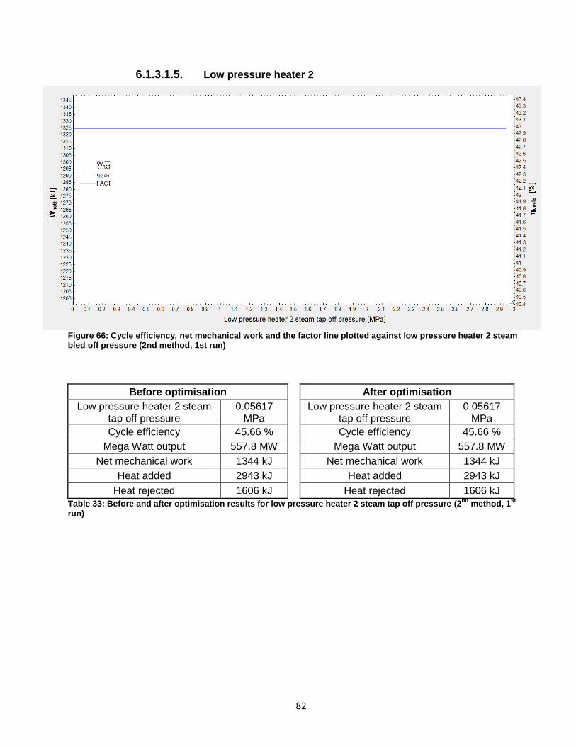
82
6.1.3.1.5. Low pressure heater 2
Figure 66: Cycle efficiency, net mechanical work and the factor line plotted against low pressure heater 2 steam bled off pressure (2nd method, 1st run)
Before optimisation
After optimisation
Low pressure heater 2 steam tap off pressure
0.05617 MPa
Low pressure heater 2 steam tap off pressure
0.05617 MPa
Cycle efficiency 45.66 %
Cycle efficiency 45.66 %
Mega Watt output 557.8 MW
Mega Watt output 557.8 MW
Net mechanical work 1344 kJ
Net mechanical work 1344 kJ
Heat added 2943 kJ
Heat added 2943 kJ
Heat rejected 1606 kJ
Heat rejected 1606 kJ
Table 33: Before and after optimisation results for low pressure heater 2 steam tap off pressure (2nd
method, 1st
run)

83
6.1.3.1.6. Low pressure heater 3
Figure 67: Cycle efficiency, net mechanical work and the factor line plotted against low pressure heater 3 steam bled off pressure (2nd method, 1st run)
Before optimisation
After optimisation
Low pressure heater 3 steam tap off pressure
0.2542 MPa
Low pressure heater 3 steam tap off pressure
0.2575 MPa
Cycle efficiency 45.66 %
Cycle efficiency 45.66 %
Mega Watt output 557.8 MW
Mega Watt output 557.8 MW
Net mechanical work 1344 kJ
Net mechanical work 1344 kJ
Heat added 2943 kJ
Heat added 2943 kJ
Heat rejected 1606 kJ
Heat rejected 1606 kJ
Table 34: Before and after optimisation results for low pressure heater 3 steam tap off pressure (2nd
method, 1st
run)

84
6.1.3.1.7. Low pressure heater 4
Figure 68: Cycle efficiency, net mechanical work and the factor line plotted against low pressure heater 4 steam bled off pressure (2nd method, 1st run)
Before optimisation
After optimisation
Low pressure heater 4 steam tap off pressure
1.971 MPa
Low pressure heater 4 steam tap off pressure
0.3794 MPa
Cycle efficiency 45.66 %
Cycle efficiency 45.97 %
Mega Watt output 557.8 MW
Mega Watt output 561.5 MW
Net mechanical work 1344 kJ
Net mechanical work 1353 kJ
Heat added 2943 kJ
Heat added 2943 kJ
Heat rejected 1606 kJ
Heat rejected 1591 kJ
Table 35: Before and after optimisation results for low pressure heater 4 steam tap off pressure (2nd
method, 1st
run)

85
6.1.3.1.8. De-aerator
Figure 69: Cycle efficiency, net mechanical work and the factor line plotted against the de-aerator steam bled off pressure (2nd method, 1st run)
Before optimisation
After optimisation
De-aerator steam tap off pressure
1.971 MPa
De-aerator steam tap off pressure
1.97 MPa
Cycle efficiency 45.97 %
Cycle efficiency 45.96 %
Mega Watt output 561.5 MW
Mega Watt output 561.5 MW
Net mechanical work 1353 kJ
Net mechanical work 1353 kJ
Heat added 2943 kJ
Heat added 2943 kJ
Heat rejected 1591 kJ
Heat rejected 1591 kJ
Table 36: Before and after optimisation results for the de-aerator steam tap off pressure (2nd
method, 1st
run)

86
6.1.3.2. Second run
6.1.3.2.1. Boiler feed pump pressure
Figure 70: Cycle efficiency, net mechanical work and the factor line plotted against boiler feed pump discharge pressure (2nd method, 2nd run)
Figure 71: Cycle efficiency, net mechanical work and the factor line plotted against boiler feed pump discharge pressure (Zoomed in) (2nd method, 2nd run)

87
Before optimisation
After optimisation
Boiler feed pump pressure 24.3 MPa
Boiler feed pump pressure 25.96 MPa
Cycle efficiency 45.96 %
Cycle efficiency 45.58%
Mega Watt output 561.5 MW
Mega Watt output 549.9 MW
Net mechanical work 1353 kJ
Net mechanical work 1325 kJ
Heat added 2943 kJ
Heat added 2907 kJ
Heat rejected 1591 kJ
Heat rejected 1585 kJ
Table 37: Before and after optimisation results for the boiler feed pump discharge (2nd
method, 2nd
run)
6.1.3.2.2. High pressure heater 6
Figure 72: Cycle efficiency, net mechanical work and the factor line plotted against the high pressure heater 6 steam tap off pressure (2nd method, 2nd run)
Before optimisation
After optimisation
High pressure heater 6 steam bled off pressure
1.838 MPa
High pressure heater 6 steam bled off pressure
2.087 MPa
Cycle efficiency 45.58%
Cycle efficiency 45.76%
Mega Watt output 549.9 MW
Mega Watt output 553.8 MW
Net mechanical work 1325 kJ
Net mechanical work 1335 kJ
Heat added 2907 kJ
Heat added 2917 kJ
Heat rejected 1585 kJ
Heat rejected 1589 kJ
Table 38: Before and after optimisation results for high pressure heater 6 steam tap off pressure (2nd
method, 2nd
run)
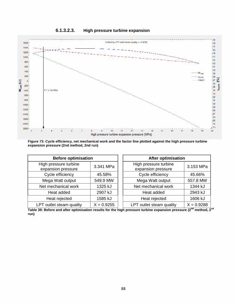
88
6.1.3.2.3. High pressure turbine expansion
Figure 73: Cycle efficiency, net mechanical work and the factor line plotted against the high pressure turbine expansion pressure (2nd method, 2nd run)
Before optimisation
After optimisation
High pressure turbine expansion pressure
3.341 MPa
High pressure turbine expansion pressure
3.153 MPa
Cycle efficiency 45.58%
Cycle efficiency 45.66%
Mega Watt output 549.9 MW
Mega Watt output 557.8 MW
Net mechanical work 1325 kJ
Net mechanical work 1344 kJ
Heat added 2907 kJ
Heat added 2943 kJ
Heat rejected 1585 kJ
Heat rejected 1606 kJ
LPT outlet steam quality X = 0.9255 LPT outlet steam quality X = 0.9288 Table 39: Before and after optimisation results for the high pressure turbine expansion pressure (2
nd method, 2
nd
run)

89
6.1.3.2.4. Low pressure heater 1
Figure 74: Cycle efficiency, net mechanical work and the factor line plotted against low pressure heater 1 steam bled off pressure (2nd method, 2nd run)
Before optimisation
After optimisation
Low pressure heater 1 steam bled off pressure
0.02779 MPa
Low pressure heater 1 steam bled off pressure
0.02779 MPa
Cycle efficiency 45.66%
Cycle efficiency 45.66%
Mega Watt output 557.8 MW
Mega Watt output 557.8 MW
Net mechanical work 1344 kJ
Net mechanical work 1344 kJ
Heat added 2943 kJ
Heat added 2943 kJ
Heat rejected 1606 kJ
Heat rejected 1606 kJ Table 40: Before and after optimisation results for low pressure heater 1 steam tap off pressure (2
nd method, 2
nd
run)

90
6.1.3.2.5. Low pressure heater 2
Figure 75: Cycle efficiency, net mechanical work and the factor line plotted against low pressure heater 2 steam bled off pressure (2nd method, 2nd run)
Before optimisation
After optimisation
Low pressure heater 2 steam bled off pressure
0.05617 MPa
Low pressure heater 2 steam bled off pressure
0.05617 MPa
Cycle efficiency 45.66%
Cycle efficiency 45.66%
Mega Watt output 557.8 MW
Mega Watt output 557.8 MW
Net mechanical work 1344 kJ
Net mechanical work 1344 kJ
Heat added 2943 kJ
Heat added 2943 kJ
Heat rejected 1606 kJ
Heat rejected 1606 kJ Table 41: Before and after optimisation results for low pressure heater 2 steam tap off pressure (2
nd method, 2
nd
run)

91
6.1.3.2.6. Low pressure heater 3
Figure 76: Cycle efficiency, net mechanical work and the factor line plotted against low pressure heater 3 steam bled off pressure (2nd method, 2nd run)
Before optimisation
After optimisation
Low pressure heater 3 steam bled off pressure
0.2542 MPa
Low pressure heater 3 steam bled off pressure
0.2541 MPa
Cycle efficiency 45.66%
Cycle efficiency 45.66%
Mega Watt output 557.8 MW
Mega Watt output 557.8 MW
Net mechanical work 1344 kJ
Net mechanical work 1344 kJ
Heat added 2943 kJ
Heat added 2943 kJ
Heat rejected 1606 kJ
Heat rejected 1606 kJ Table 42: Before and after optimisation results for low pressure heater 3 steam tap off pressure (2
nd method, 2
nd
run)

92
6.1.3.2.7. Low pressure heater 4
Figure 77: Cycle efficiency, net mechanical work and the factor line plotted against low pressure heater 4 steam bled off pressure (2nd method, 2nd run)
Before optimisation
After optimisation
Low pressure heater 4 steam bled off pressure
1.971 MPa
Low pressure heater 4 steam bled off pressure
0.3794 MPa
Cycle efficiency 45.66%
Cycle efficiency 45.97%
Mega Watt output 557.8 MW
Mega Watt output 561.5 MW
Net mechanical work 1344 kJ
Net mechanical work 1353 kJ
Heat added 2943 kJ
Heat added 2943 kJ
Heat rejected 1606 kJ
Heat rejected 1591 kJ Table 43: Before and after optimisation results for low pressure heater 4 steam tap off pressure (2
nd method, 2
nd
run)
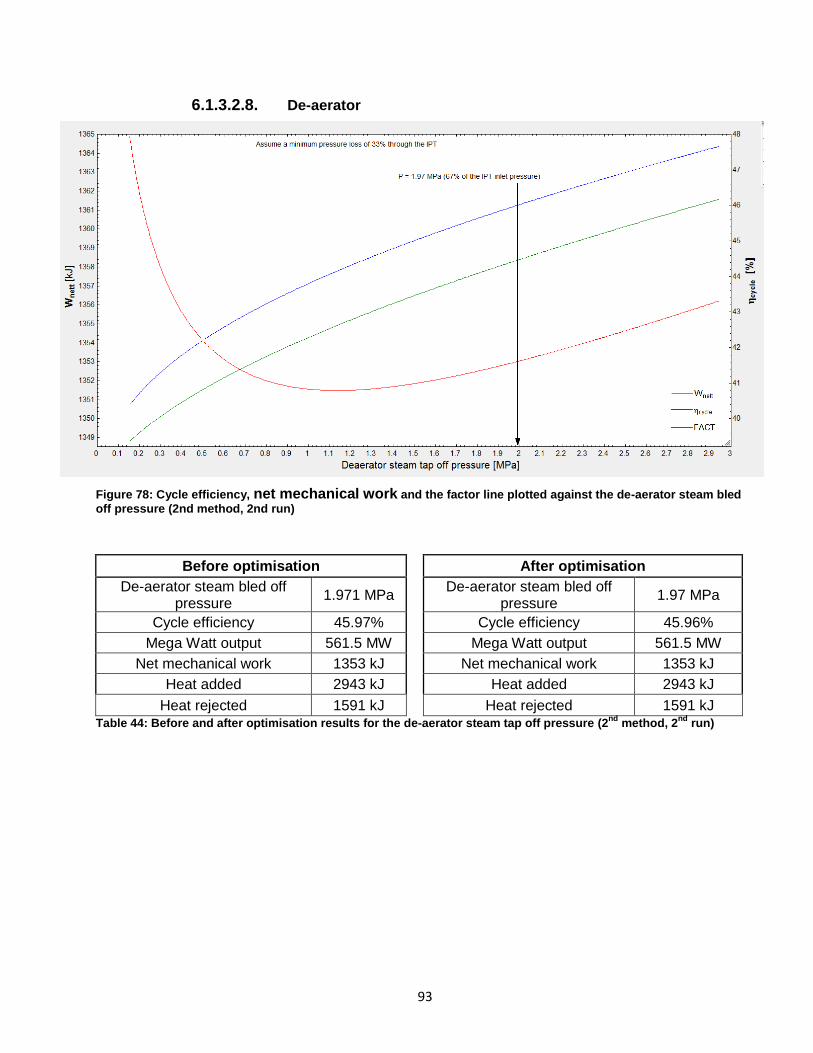
93
6.1.3.2.8. De-aerator
Figure 78: Cycle efficiency, net mechanical work and the factor line plotted against the de-aerator steam bled
off pressure (2nd method, 2nd run)
Before optimisation
After optimisation
De-aerator steam bled off pressure
1.971 MPa
De-aerator steam bled off pressure
1.97 MPa
Cycle efficiency 45.97%
Cycle efficiency 45.96%
Mega Watt output 561.5 MW
Mega Watt output 561.5 MW
Net mechanical work 1353 kJ
Net mechanical work 1353 kJ
Heat added 2943 kJ
Heat added 2943 kJ
Heat rejected 1591 kJ
Heat rejected 1591 kJ Table 44: Before and after optimisation results for the de-aerator steam tap off pressure (2
nd method, 2
nd run)

94
6.1.3.3. Third run
6.1.3.3.1. Boiler feed pump pressure
Figure 79: Cycle efficiency, net mechanical work and the factor line plotted against boiler feed pump discharge pressure (2nd method, 3rd run)
Figure 80: Cycle efficiency, net mechanical work and the factor line plotted against boiler feed pump discharge pressure (Zoomed in) (2nd method, 3rd run)

95
Before optimisation
After optimisation
Boiler feed pump pressure 25.96 MPa
Boiler feed pump pressure 29.17 MPa
Cycle efficiency 45.96%
Cycle efficiency 46.25%
Mega Watt output 561.5 MW
Mega Watt output 558.3 MW
Net mechanical work 1353 kJ
Net mechanical work 1345 kJ
Heat added 2943 kJ
Heat added 2909 kJ
Heat rejected 1591 kJ
Heat rejected 1567 kJ Table 45: Before and after optimisation results for the boiler feed pump discharge (2
nd method, 3
rd run)
6.1.3.3.2. High pressure heater 6
Figure 81: Cycle efficiency, net mechanical work and the factor line plotted against the high pressure heater 6 steam tap off pressure (2nd method, 3rd run)
Before optimisation
After optimisation
High pressure heater 6 steam tap off pressure
2.137 MPa
High pressure heater 6 steam tap off pressure
2.137 MPa
Cycle efficiency 46.25%
Cycle efficiency 46.25%
Mega Watt output 558.3 MW
Mega Watt output 558.3 MW
Net mechanical work 1345 kJ
Net mechanical work 1345 kJ
Heat added 2909 kJ
Heat added 2909 kJ
Heat rejected 1567 kJ
Heat rejected 1567 kJ Table 46: Before and after optimisation results for high pressure heater 6 steam tap off pressure (2
nd method, 3
rd
run)

96
6.1.3.3.3. High pressure turbine expansion
Figure 82: Cycle efficiency, net mechanical work and the factor line plotted against the high pressure turbine expansion pressure (2nd method, 3rd run)
Before optimisation
After optimisation
High pressure turbine expansion pressure
3.42 MPa
High pressure turbine expansion pressure
3.146 MPa
Cycle efficiency 46.25%
Cycle efficiency 46.08%
Mega Watt output 558.3 MW
Mega Watt output 563.5 MW
Net mechanical work 1345 kJ
Net mechanical work 1358 kJ
Heat added 2909 kJ
Heat added 2947 kJ
Heat rejected 1567 kJ
Heat rejected 1592 kJ
LPT outlet steam quality X = 0.9242 LPT outlet steam quality X = 0.9288 Table 47: Before and after optimisation results for the high pressure turbine expansion pressure (2
nd method, 3
rd
run)
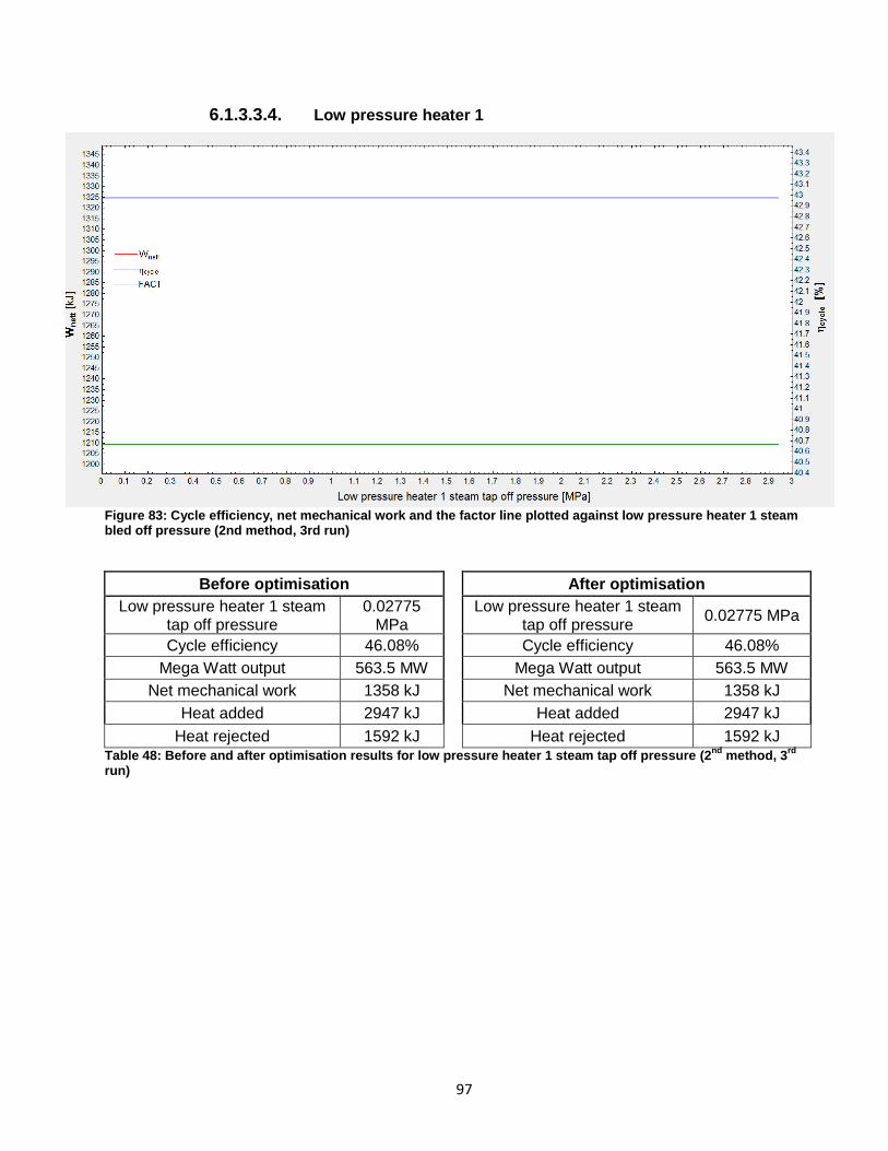
97
6.1.3.3.4. Low pressure heater 1
Figure 83: Cycle efficiency, net mechanical work and the factor line plotted against low pressure heater 1 steam bled off pressure (2nd method, 3rd run)
Before optimisation
After optimisation
Low pressure heater 1 steam tap off pressure
0.02775 MPa
Low pressure heater 1 steam tap off pressure
0.02775 MPa
Cycle efficiency 46.08%
Cycle efficiency 46.08%
Mega Watt output 563.5 MW
Mega Watt output 563.5 MW
Net mechanical work 1358 kJ
Net mechanical work 1358 kJ
Heat added 2947 kJ
Heat added 2947 kJ
Heat rejected 1592 kJ
Heat rejected 1592 kJ Table 48: Before and after optimisation results for low pressure heater 1 steam tap off pressure (2
nd method, 3
rd
run)

98
6.1.3.3.5. Low pressure heater 2
Figure 84: Cycle efficiency, net mechanical work and the factor line plotted against low pressure heater 2 steam bled off pressure (2nd method, 3rd run)
Before optimisation
After optimisation
Low pressure heater 2 steam tap off pressure
0.05609 MPa
Low pressure heater 2 steam tap off pressure
0.05609 MPa
Cycle efficiency 46.08%
Cycle efficiency 46.08%
Mega Watt output 563.5 MW
Mega Watt output 563.5 MW
Net mechanical work 1358 kJ
Net mechanical work 1358 kJ
Heat added 2947 kJ
Heat added 2947 kJ
Heat rejected 1592 kJ
Heat rejected 1592 kJ Table 49: Before and after optimisation results for low pressure heater 2 steam tap off pressure (2
nd method, 3
rd
run)

99
6.1.3.3.6. Low pressure heater 3
Figure 85: Cycle efficiency, net mechanical work and the factor line plotted against low pressure heater 3 steams bled off pressure (2nd method, 3rd run)
Before optimisation
After optimisation
Low pressure heater 3 steam tap off pressure
0.2537 MPa
Low pressure heater 3 steam tap off pressure
0.2537 MPa
Cycle efficiency 46.08%
Cycle efficiency 46.08%
Mega Watt output 563.5 MW
Mega Watt output 563.5 MW
Net mechanical work 1358 kJ
Net mechanical work 1358 kJ
Heat added 2947 kJ
Heat added 2947 kJ
Heat rejected 1592 kJ
Heat rejected 1592 kJ Table 50: Before and after optimisation results for low pressure heater 3 steam tap off pressure (2
nd method, 3
rd
run)
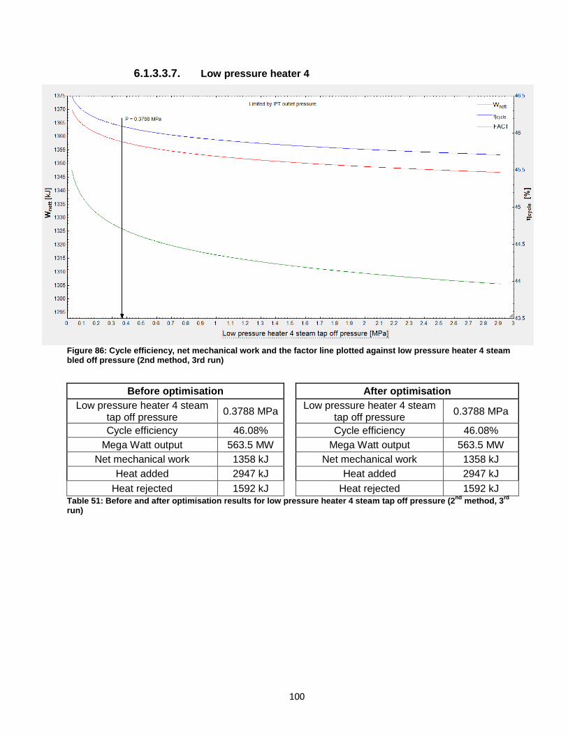
100
6.1.3.3.7. Low pressure heater 4
Figure 86: Cycle efficiency, net mechanical work and the factor line plotted against low pressure heater 4 steam bled off pressure (2nd method, 3rd run)
Before optimisation
After optimisation
Low pressure heater 4 steam tap off pressure
0.3788 MPa
Low pressure heater 4 steam tap off pressure
0.3788 MPa
Cycle efficiency 46.08%
Cycle efficiency 46.08%
Mega Watt output 563.5 MW
Mega Watt output 563.5 MW
Net mechanical work 1358 kJ
Net mechanical work 1358 kJ
Heat added 2947 kJ
Heat added 2947 kJ
Heat rejected 1592 kJ
Heat rejected 1592 kJ Table 51: Before and after optimisation results for low pressure heater 4 steam tap off pressure (2
nd method, 3
rd
run)
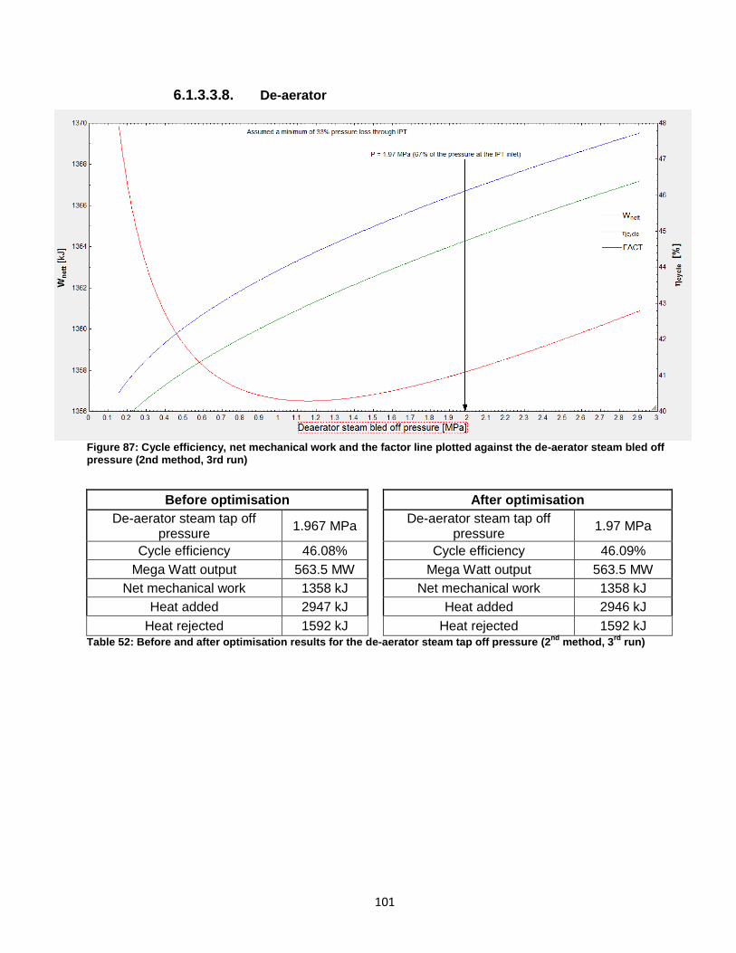
101
6.1.3.3.8. De-aerator
Figure 87: Cycle efficiency, net mechanical work and the factor line plotted against the de-aerator steam bled off pressure (2nd method, 3rd run)
Before optimisation
After optimisation
De-aerator steam tap off pressure
1.967 MPa
De-aerator steam tap off pressure
1.97 MPa
Cycle efficiency 46.08%
Cycle efficiency 46.09%
Mega Watt output 563.5 MW
Mega Watt output 563.5 MW
Net mechanical work 1358 kJ
Net mechanical work 1358 kJ
Heat added 2947 kJ
Heat added 2946 kJ
Heat rejected 1592 kJ
Heat rejected 1592 kJ Table 52: Before and after optimisation results for the de-aerator steam tap off pressure (2
nd method, 3
rd run)

102
6.1.3.3.9. Boiler feed pump
Figure 88: Cycle efficiency, net mechanical work and the factor line plotted against boiler feed pump discharge pressure (2nd method, 4th run)
Figure 89: Cycle efficiency, net mechanical work and the factor line plotted against boiler feed pump discharge pressure (zoomed in) (2nd method, 4th run)

103
Before optimisation
After optimisation
Boiler feed pump pressure 29.17 MPa
Boiler feed pump pressure 29.27 MPa
Cycle efficiency 46.09%
Cycle efficiency 46.1%
Mega Watt output 563.5 MW
Mega Watt output 563.4 MW
Net mechanical work 1358 kJ
Net mechanical work 1358 kJ
Heat added 2946 kJ
Heat added 2945 kJ
Heat rejected 1592 kJ
Heat rejected 1592 kJ Table 53: Before and after optimisation results for the boiler feed pump discharge (2
nd method, 4
th run)
6.1.3.3.10. High pressure turbine expansion
Figure 90: Cycle efficiency, net mechanical work and the factor line plotted against the high pressure turbine expansion pressure (2nd method, 4th run)
Before optimisation
After optimisation
High pressure turbine expansion pressure
3.154 MPa
High pressure turbine expansion pressure
3.15 MPa
Cycle efficiency 46.1%
Cycle efficiency 46.1%
Mega Watt output 563.4 MW
Mega Watt output 563.5 MW
Net mechanical work 1358 kJ
Net mechanical work 1358 kJ
Heat added 2945 kJ
Heat added 2946 kJ
Heat rejected 1592 kJ
Heat rejected 1592 kJ
LPT outlet steam quality X = 0.9287 LPT outlet steam quality X = 0.9288 Table 54: Before and after optimisation results for the high pressure turbine expansion pressure (2
nd method, 4
th
run)

104
6.1.4. Adjustments after sub-critical cycle was optimised
After optimisation the first and second methods produced the same results.
The result of the tap off steam flow for high pressure heater 6 was negative, which means that
steam was flowing back into the intermediate pressure turbine. Thus high pressure heater 6
was no longer necessary and was removed. The cycle was calculated again and the following
results were obtained. For this section the steam tap off flow m_6 is equal to 0.
After high pressure heater 6 was taken out
Maximum boiler pressure 3.154 MPa
Cycle efficiency 46.34%
Mega Watt output 569.2 MW
Net mechanical work 1372 kJ
Heat added 2960 kJ
Heat rejected 1600 kJ Table 55: Results for sub-critical cycle after optimisation and after high pressure heater 6 was taken out
Figure 91: Sub-critical plant layout with steam flows, after high pressure heater 6 was taken out
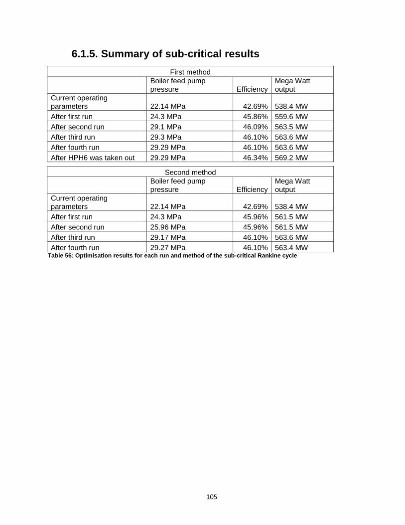
105
6.1.5. Summary of sub-critical results
First method
Boiler feed pump pressure Efficiency
Mega Watt output
Current operating parameters 22.14 MPa 42.69% 538.4 MW
After first run 24.3 MPa 45.86% 559.6 MW
After second run 29.1 MPa 46.09% 563.5 MW
After third run 29.3 MPa 46.10% 563.6 MW
After fourth run 29.29 MPa 46.10% 563.6 MW
After HPH6 was taken out 29.29 MPa 46.34% 569.2 MW
Second method
Boiler feed pump pressure Efficiency
Mega Watt output
Current operating parameters 22.14 MPa 42.69% 538.4 MW
After first run 24.3 MPa 45.96% 561.5 MW
After second run 25.96 MPa 45.96% 561.5 MW
After third run 29.17 MPa 46.10% 563.6 MW
After fourth run 29.27 MPa 46.10% 563.4 MW Table 56: Optimisation results for each run and method of the sub-critical Rankine cycle

106
6.2. Super-critical optimisation results The super-critical cycle was based on the heat balance diagrams from Medupi power station at
794MW output
6.2.1. Super-critical cycle without optimisation
6.2.1.1. Input parameters
The input parameters were taken from the original heat balance diagram for Medupi power station.
Table 57: Super-critical Rankine cycle input parameters
6.2.1.2. Results
This is the current Rankine cycle as it is on the heat balance diagram of Medupi Power station
Table 58: Results for super-critical cycle with input parameters before optimisation
Feed pump 30.13 MPa
Maximum Temperature 570°C
Minimum Temperature 50°C
Maximum mass flow 635 kg/s
Extraction pump discharge pressure 2.5 MPa
High pressure heater 6 bled steam tap off pressure 2.745 MPa
De-aerator bled steam tap off pressure 1.12 MPa
Low pressure heater 3 bled steam tap off pressure 0.591 MPa
Low pressure heater 2 bled steam tap off pressure 0.2671 MPa
Low pressure heater 1 bled steam tap off pressure 0.09048 MPa
Cycle efficiency 42.31 %
Mega Watt out 831.6 MW
Total Work in 38.65 kJ
Total Work out 1348 kJ
Net mechanical work 1310 kJ
Heat added 3096 kJ
Heat rejected 1495 kJ

107
Figure 92: Current super-critical Rankine cycle before any optimisation
Figure 93: Plant layout at Medupi power station (super-critical)

108
6.2.2. Super-critical cycle optimisation – first method
6.2.2.1. First run
6.2.2.1.1. Boiler feed pump pressure
Figure 94: Cycle efficiency, net mechanical work and the factor line plotted against boiler feed pump discharge pressure (1st method, 1st run)
Figure 95: Cycle efficiency, net mechanical work and the factor line plotted against boiler feed pump discharge pressure (Zoomed in) (1st method, 1st run)
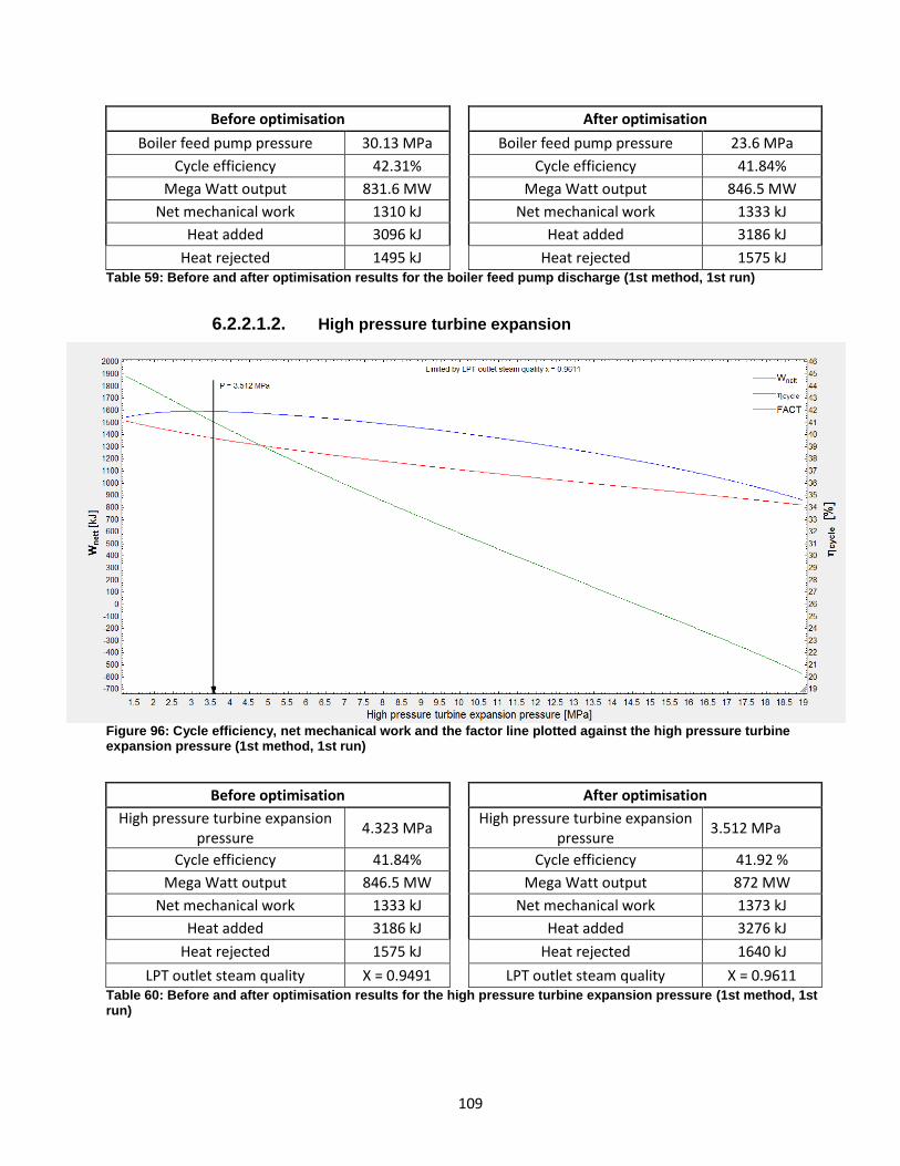
109
Before optimisation
After optimisation
Boiler feed pump pressure 30.13 MPa
Boiler feed pump pressure 23.6 MPa
Cycle efficiency 42.31%
Cycle efficiency 41.84%
Mega Watt output 831.6 MW
Mega Watt output 846.5 MW
Net mechanical work 1310 kJ
Net mechanical work 1333 kJ
Heat added 3096 kJ
Heat added 3186 kJ
Heat rejected 1495 kJ
Heat rejected 1575 kJ Table 59: Before and after optimisation results for the boiler feed pump discharge (1st method, 1st run)
6.2.2.1.2. High pressure turbine expansion
Figure 96: Cycle efficiency, net mechanical work and the factor line plotted against the high pressure turbine expansion pressure (1st method, 1st run)
Before optimisation
After optimisation
High pressure turbine expansion pressure
4.323 MPa
High pressure turbine expansion pressure
3.512 MPa
Cycle efficiency 41.84%
Cycle efficiency 41.92 %
Mega Watt output 846.5 MW
Mega Watt output 872 MW
Net mechanical work 1333 kJ
Net mechanical work 1373 kJ
Heat added 3186 kJ
Heat added 3276 kJ
Heat rejected 1575 kJ
Heat rejected 1640 kJ
LPT outlet steam quality X = 0.9491 LPT outlet steam quality X = 0.9611 Table 60: Before and after optimisation results for the high pressure turbine expansion pressure (1st method, 1st run)

110
6.2.2.1.3. High pressure heater 6
Figure 97: Cycle efficiency, net mechanical work and the factor line plotted against the high pressure heater 6 steam tap off pressure (1st method, 1st run)
Before optimisation
After optimisation
High pressure heater 6 steam bled off pressure
1.755 MPa
High pressure heater 6 steam bled off pressure
2.16 MPa
Cycle efficiency 41.92 %
Cycle efficiency 42.25 %
Mega Watt output 872 MW
Mega Watt output 882.8 MW
Net mechanical work 1373 kJ
Net mechanical work 1390 kJ
Heat added 3276 kJ
Heat added 3291 kJ
Heat rejected 1640 kJ
Heat rejected 1651 kJ Table 61: Before and after optimisation results for high pressure heater 6 steam tap off pressure (1st method, 1st run)

111
6.2.2.1.4. De-aerator
Figure 98: Cycle efficiency, net mechanical work and the factor line plotted against the de-aerator steam bled off pressure (1st method, 1st run)
Before optimisation
After optimisation
De-aerator steam bled off pressure
0.7161 MPa
De-aerator steam bled off pressure
2.16 MPa
Cycle efficiency 42.25 %
Cycle efficiency 45.37 %
Mega Watt output 882.8 MW
Mega Watt output 883.1 MW
Net mechanical work 1390 kJ
Net mechanical work 1391 kJ
Heat added 3291 kJ
Heat added 3065 kJ
Heat rejected 1651 kJ
Heat rejected 1653 kJ Table 62: Before and after optimisation results for the de-aerator steam tap off pressure (1st method, 1st run)
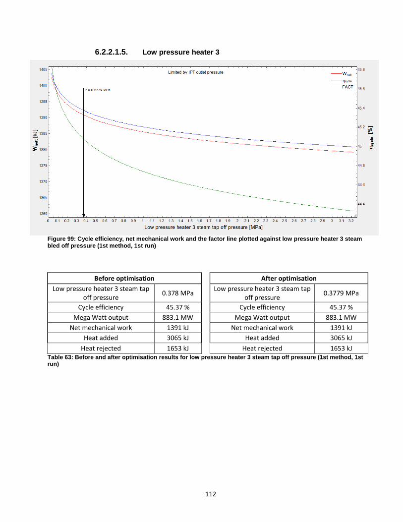
112
6.2.2.1.5. Low pressure heater 3
Figure 99: Cycle efficiency, net mechanical work and the factor line plotted against low pressure heater 3 steam bled off pressure (1st method, 1st run)
Before optimisation
After optimisation
Low pressure heater 3 steam tap off pressure
0.378 MPa
Low pressure heater 3 steam tap off pressure
0.3779 MPa
Cycle efficiency 45.37 %
Cycle efficiency 45.37 %
Mega Watt output 883.1 MW
Mega Watt output 883.1 MW
Net mechanical work 1391 kJ
Net mechanical work 1391 kJ
Heat added 3065 kJ
Heat added 3065 kJ
Heat rejected 1653 kJ
Heat rejected 1653 kJ Table 63: Before and after optimisation results for low pressure heater 3 steam tap off pressure (1st method, 1st run)
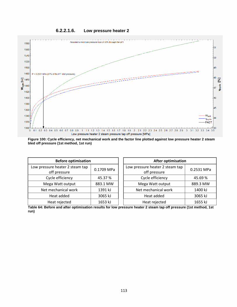
113
6.2.2.1.6. Low pressure heater 2
Figure 100: Cycle efficiency, net mechanical work and the factor line plotted against low pressure heater 2 steam bled off pressure (1st method, 1st run)
Before optimisation
After optimisation
Low pressure heater 2 steam tap off pressure
0.1709 MPa
Low pressure heater 2 steam tap off pressure
0.2531 MPa
Cycle efficiency 45.37 %
Cycle efficiency 45.69 %
Mega Watt output 883.1 MW
Mega Watt output 889.3 MW
Net mechanical work 1391 kJ
Net mechanical work 1400 kJ
Heat added 3065 kJ
Heat added 3065 kJ
Heat rejected 1653 kJ
Heat rejected 1655 kJ Table 64: Before and after optimisation results for low pressure heater 2 steam tap off pressure (1st method, 1st run)

114
6.2.2.1.7. Low pressure heater 1
Figure 101: Cycle efficiency, net mechanical work and the factor line plotted against low pressure heater 1 steam bled off pressure (1st method, 1st run)
Before optimisation
After optimisation
Low pressure heater 1 steam tap off pressure
0.05787 MPa
Low pressure heater 1 steam tap off pressure
0.05787 MPa
Cycle efficiency 45.69 %
Cycle efficiency 45.69 %
Mega Watt output 889.3 MW
Mega Watt output 889.3 MW
Net mechanical work 1400 kJ
Net mechanical work 1400 kJ
Heat added 3065 kJ
Heat added 3065 kJ
Heat rejected 1655 kJ
Heat rejected 1655 kJ Table 65: Before and after optimisation results for low pressure heater 1 steam tap off pressure (1st method, 1st run)

115
6.2.2.2. Second run
6.2.2.2.1. Boiler feed pump pressure
Figure 102: Cycle efficiency, net mechanical work and the factor line plotted against boiler feed pump discharge pressure (1st method, 2nd run)
Figure 103: Cycle efficiency, net-work and the factor line plotted against boiler feed pump discharge pressure (zoomed in) (1st method, 2nd run)

116
Before optimisation
After optimisation
Boiler feed pump pressure 23.6 MPa
Boiler feed pump pressure 31.47 MPa
Cycle efficiency 45.69 %
Cycle efficiency 46.79 %
Mega Watt output 889.3 MW
Mega Watt output 875.3 MW
Net mechanical work 1400 kJ
Net mechanical work 1378 kJ
Heat added 3065 kJ
Heat added 2946 kJ
Heat rejected 1655 kJ
Heat rejected 1565 kJ Table 66: Before and after optimisation results for the boiler feed pump discharge (1
st method, 2
nd run)
6.2.2.2.2. High pressure turbine expansion
Figure 104: Cycle efficiency, net mechanical work and the factor line plotted against the high pressure turbine expansion pressure (1st method, 2nd run)
Before optimisation
After optimisation
High pressure turbine expansion pressure
4.66 MPa
High pressure turbine expansion pressure
3.505 MPa
Cycle efficiency 46.79 %
Cycle efficiency 46.25 %
Mega Watt output 875.3 MW
Mega Watt output 905.6 MW
Net mechanical work 1378 kJ
Net mechanical work 1426 kJ
Heat added 2946 kJ
Heat added 3083 kJ
Heat rejected 1565 kJ
Heat rejected 1656 kJ
LPT outlet steam quality X = 0.9446 LPT outlet steam quality X = 0.9611 Table 67: Before and after optimisation results for the high pressure turbine expansion pressure (1
st method, 2
nd
run)

117
6.2.2.2.3. High pressure heater 6
Figure 105: Cycle efficiency, net mechanical work and the factor line plotted against the high pressure heater 6 steam tap off pressure (1st method, 1st run)
Before optimisation
After optimisation
High pressure heater 6 steam bled off pressure
2.161 MPa
High pressure heater 6 steam bled off pressure
2.16 MPa
Cycle efficiency 46.25 %
Cycle efficiency 46.25 %
Mega Watt output 905.6 MW
Mega Watt output 905.6 MW
Net mechanical work 1426 kJ
Net mechanical work 1426 kJ
Heat added 3083 kJ
Heat added 3083 kJ
Heat rejected 1656 kJ
Heat rejected 1656 kJ Table 68: Before and after optimisation results for high pressure heater 6 steam tap off pressure (1
st method, 2
nd
run)

118
6.2.2.2.4. De-aerator
Figure 106: Cycle efficiency, net mechanical work and the factor line plotted against the de-aerator steam bled off pressure (1st method, 2nd run)
Before optimisation
After optimisation
De-aerator steam bled off pressure
2.161 MPa
De-aerator steam bled off pressure
2.161 MPa
Cycle efficiency 46.25 %
Cycle efficiency 46.25 %
Mega Watt output 905.6 MW
Mega Watt output 905.6 MW
Net mechanical work 1426 kJ
Net mechanical work 1426 kJ
Heat added 3083 kJ
Heat added 3084 kJ
Heat rejected 1656 kJ
Heat rejected 1656 kJ Table 69: Before and after optimisation results for the de-aerator steam tap off pressure (1
st method, 2
nd run)

119
6.2.2.2.5. Low pressure heater 3
Figure 107: Cycle efficiency, net mechanical work and the factor line plotted against low pressure heater 3 steam bled off pressure (1st method, 2nd run)
Before optimisation
After optimisation
Low pressure heater 3 steam tap off pressure
0.378 MPa
Low pressure heater 3 steam tap off pressure
0.378 MPa
Cycle efficiency 46.25 %
Cycle efficiency 46.25 %
Mega Watt output 905.6 MW
Mega Watt output 905.6 MW
Net mechanical work 1426 kJ
Net mechanical work 1426 kJ
Heat added 3084 kJ
Heat added 3084 kJ
Heat rejected 1656 kJ
Heat rejected 1656 kJ Table 70: Before and after optimisation results for low pressure heater 3 steam tap off pressure (1
st method, 2
nd
run)

120
6.2.2.2.6. Low pressure heater 2
Figure 108: Cycle efficiency, net mechanical work and the factor line plotted against low pressure heater 2 steam bled off pressure (2nd method, 2nd run)
Before optimisation
After optimisation
Low pressure heater 2 steam tap off pressure
0.2532 MPa
Low pressure heater 2 steam tap off pressure
0.378 MPa
Cycle efficiency 46.25 %
Cycle efficiency 46.25 %
Mega Watt output 905.6 MW
Mega Watt output 905.6 MW
Net mechanical work 1426 kJ
Net mechanical work 1426 kJ
Heat added 3084 kJ
Heat added 3084 kJ
Heat rejected 1656 kJ
Heat rejected 1656 kJ Table 71: Before and after optimisation results for low pressure heater 2 steam tap off pressure (1
st method, 2
nd
run)

121
6.2.2.2.7. Low pressure heater 1
Figure 109: Cycle efficiency, net mechanical work and the factor line plotted against low pressure heater 1 steam bled off pressure (1st method, 2nd run)
Before optimisation
After optimisation
Low pressure heater 1 steam tap off pressure
0.0579 MPa
Low pressure heater 1 steam tap off pressure
0.0579 MPa
Cycle efficiency 46.25 %
Cycle efficiency 46.25 %
Mega Watt output 905.6 MW
Mega Watt output 905.6 MW
Net mechanical work 1426 kJ
Net mechanical work 1426 kJ
Heat added 3084 kJ
Heat added 3084 kJ
Heat rejected 1656 kJ
Heat rejected 1656 kJ Table 72: Before and after optimisation results for low pressure heater 4 steam tap off pressure (1
st method, 2
nd
run)

122
6.2.2.3. Third run
6.2.2.3.1. Boiler feed pump pressure
Figure 110: Cycle efficiency, net mechanical work and the factor line plotted against boiler feed pump discharge pressure (1st method, 3rd run)
Figure 111: Cycle efficiency, net mechanical work and the factor line plotted against boiler feed pump discharge pressure (zoomed in) (1st method, 3rd run)

123
Before optimisation
After optimisation
Boiler feed pump pressure 31.47 MPa
Boiler feed pump pressure 31.99 MPa
Cycle efficiency 46.25 %
Cycle efficiency 46.3 %
Mega Watt output 905.6 MW
Mega Watt output 904.6 MW
Net mechanical work 1426 kJ
Net mechanical work 1425 kJ
Heat added 3084 kJ
Heat added 3077 kJ
Heat rejected 1656 kJ
Heat rejected 1651 kJ Table 73: Before and after optimisation results for the boiler feed pump discharge (1
st method, 3
rd run)
6.2.2.3.2. High pressure turbine expansion
Figure 112: Cycle efficiency, net mechanical work and the factor line plotted against the high pressure turbine expansion pressure (1st method, 3rd run)
Before optimisation
After optimisation
High pressure turbine expansion pressure
3.56 MPa
High pressure turbine expansion pressure
3.499 MPa
Cycle efficiency 46.3 %
Cycle efficiency 46.27 %
Mega Watt output 904.6 MW
Mega Watt output 906.3 MW
Net mechanical work 1425 kJ
Net mechanical work 1425 kJ
Heat added 3077 kJ
Heat added 3077 kJ
Heat rejected 1651 kJ
Heat rejected 1651 kJ
LPT outlet steam quality X = 0.9601 LPT outlet steam quality X = 0.9611 Table 74: Before and after optimisation results for the high pressure turbine expansion pressure (1
st method, 3
rd
run)
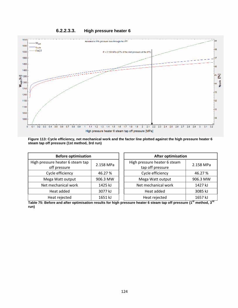
124
6.2.2.3.3. High pressure heater 6
Figure 113: Cycle efficiency, net mechanical work and the factor line plotted against the high pressure heater 6 steam tap off pressure (1st method, 3rd run)
Before optimisation
After optimisation
High pressure heater 6 steam tap off pressure
2.158 MPa
High pressure heater 6 steam tap off pressure
2.158 MPa
Cycle efficiency 46.27 %
Cycle efficiency 46.27 %
Mega Watt output 906.3 MW
Mega Watt output 906.3 MW
Net mechanical work 1425 kJ
Net mechanical work 1427 kJ
Heat added 3077 kJ
Heat added 3085 kJ
Heat rejected 1651 kJ
Heat rejected 1657 kJ Table 75: Before and after optimisation results for high pressure heater 6 steam tap off pressure (1
st method, 3
rd
run)

125
6.2.2.3.4. De-aerator
Figure 114: Cycle efficiency, net mechanical work and the factor line plotted against the de-aerator steam bled off pressure (1st method, 3rd run)
Before optimisation
After optimisation
De-aerator steam tap off pressure
2.157 MPa
De-aerator steam tap off pressure
2.157 MPa
Cycle efficiency 46.27 %
Cycle efficiency 46.27 %
Mega Watt output 906.3 MW
Mega Watt output 906.3 MW
Net mechanical work 1427 kJ
Net mechanical work 1427 kJ
Heat added 3085 kJ
Heat added 3085 kJ
Heat rejected 1657 kJ
Heat rejected 1657 kJ Table 76: Before and after optimisation results for the de-aerator steam tap off pressure (1
st method, 3
rd run)
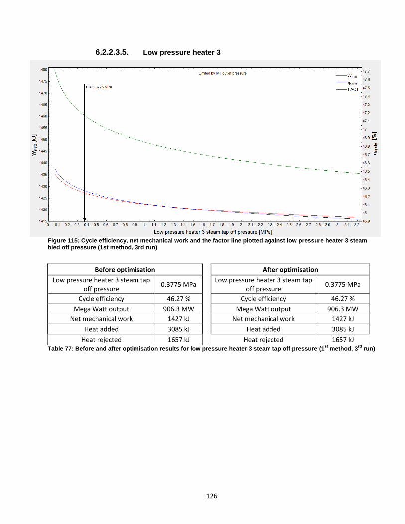
126
6.2.2.3.5. Low pressure heater 3
Figure 115: Cycle efficiency, net mechanical work and the factor line plotted against low pressure heater 3 steam bled off pressure (1st method, 3rd run)
Before optimisation
After optimisation
Low pressure heater 3 steam tap off pressure
0.3775 MPa
Low pressure heater 3 steam tap off pressure
0.3775 MPa
Cycle efficiency 46.27 %
Cycle efficiency 46.27 %
Mega Watt output 906.3 MW
Mega Watt output 906.3 MW
Net mechanical work 1427 kJ
Net mechanical work 1427 kJ
Heat added 3085 kJ
Heat added 3085 kJ
Heat rejected 1657 kJ
Heat rejected 1657 kJ Table 77: Before and after optimisation results for low pressure heater 3 steam tap off pressure (1
st method, 3
rd run)

127
6.2.2.3.6. Low pressure heater 2
Figure 116: Cycle efficiency, net mechanical work and the factor line plotted against low pressure heater 2 steam bled off pressure (2nd method, 3rd run)
Before optimisation
After optimisation
Low pressure heater 2 steam tap off pressure
0.2528 MPa
Low pressure heater 2 steam tap off pressure
0.2529 MPa
Cycle efficiency 46.27 %
Cycle efficiency 46.27 %
Mega Watt output 906.3 MW
Mega Watt output 906.3 MW
Net mechanical work 1427 kJ
Net mechanical work 1427 kJ
Heat added 3085 kJ
Heat added 3085 kJ
Heat rejected 1657 kJ
Heat rejected 1657 kJ Table 78: Before and after optimisation results for low pressure heater 2 steam tap off pressure (1
st method, 3
rd run)
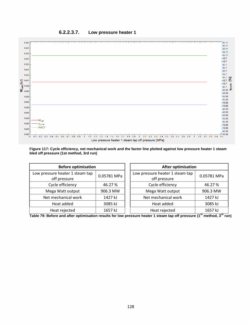
128
6.2.2.3.7. Low pressure heater 1
Figure 117: Cycle efficiency, net mechanical work and the factor line plotted against low pressure heater 1 steam bled off pressure (1st method, 3rd run)
Before optimisation
After optimisation
Low pressure heater 1 steam tap off pressure
0.05781 MPa
Low pressure heater 1 steam tap off pressure
0.05781 MPa
Cycle efficiency 46.27 %
Cycle efficiency 46.27 %
Mega Watt output 906.3 MW
Mega Watt output 906.3 MW
Net mechanical work 1427 kJ
Net mechanical work 1427 kJ
Heat added 3085 kJ
Heat added 3085 kJ
Heat rejected 1657 kJ
Heat rejected 1657 kJ Table 79: Before and after optimisation results for low pressure heater 1 steam tap off pressure (1
st method, 3
rd run)

129
6.2.2.3.8. Boiler feed pump
Figure 118: Cycle efficiency, net mechanical work and the factor line plotted against boiler feed pump discharge pressure (1st method, 4th run)
Figure 119: Cycle efficiency, net mechanical work and the factor line plotted against boiler feed pump discharge pressure (Zoomed in) (1st method, 4th run)
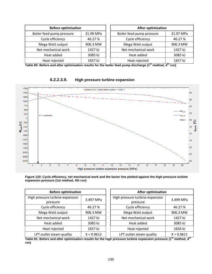
130
Before optimisation
After optimisation
Boiler feed pump pressure 31.99 MPa
Boiler feed pump pressure 31.97 MPa
Cycle efficiency 46.27 %
Cycle efficiency 46.27 %
Mega Watt output 906.3 MW
Mega Watt output 906.3 MW
Net mechanical work 1427 kJ
Net mechanical work 1427 kJ
Heat added 3085 kJ
Heat added 3085 kJ
Heat rejected 1657 kJ
Heat rejected 1657 kJ Table 80: Before and after optimisation results for the boiler feed pump discharge (1
st method, 4
th run)
6.2.2.3.9. High pressure turbine expansion
Figure 120: Cycle efficiency, net mechanical work and the factor line plotted against the high pressure turbine expansion pressure (1st method, 4th run)
Before optimisation
After optimisation
High pressure turbine expansion pressure
3.497 MPa
High pressure turbine expansion pressure
3.499 MPa
Cycle efficiency 46.27 %
Cycle efficiency 46.27 %
Mega Watt output 906.3 MW
Mega Watt output 906.3 MW
Net mechanical work 1427 kJ
Net mechanical work 1427 kJ
Heat added 3085 kJ
Heat added 3085 kJ
Heat rejected 1657 kJ
Heat rejected 1656 kJ
LPT outlet steam quality X = 0.9612 LPT outlet steam quality X = 0.9611 Table 81: Before and after optimisation results for the high pressure turbine expansion pressure (1
st method, 4
th
run)

131
6.2.3. Super-critical cycle optimisation – second method
6.2.3.1. First run
6.2.3.1.1. Boiler feed pump pressure
Figure 121: Cycle efficiency, net mechanical work and the factor line plotted against boiler feed pump discharge pressure (2nd method, 1st run)
Figure 122: Cycle efficiency, net mechanical work and the factor line plotted against boiler feed pump discharge pressure (zoomed in) (2nd method, 1st run)

132
Before optimisation
After optimisation
Boiler feed pump pressure 30.13 MPa
Boiler feed pump pressure 23.6 MPa
Cycle efficiency 42.31%
Cycle efficiency 41.84 %
Mega Watt output 831.6 MW
Mega Watt output 846.5 MW
Net mechanical work 1310 kJ
Net mechanical work 1333 kJ
Heat added 3096 kJ
Heat added 3186 kJ
Heat rejected 1495 kJ
Heat rejected 1575 kJ Table 82: Before and after optimisation results for the boiler feed pump discharge pressure (2
nd method, 1
st run)
6.2.3.1.2. High pressure heater 6
Figure 123: Cycle efficiency, net mechanical work and the factor line plotted against the high pressure heater 6 steam tap off pressure (1st method, 1st run)
Before optimisation
After optimisation
High pressure heater 6 steam tap off pressure
2.157 MPa
High pressure heater 6 steam tap off pressure
2.654 MPa
Cycle efficiency 41.84 %
Cycle efficiency 42.21 %
Mega Watt output 846.5 MW
Mega Watt output 857.9 MW
Net mechanical work 1333 kJ
Net mechanical work 1351 kJ
Heat added 3186 kJ
Heat added 3200 kJ
Heat rejected 1575 kJ
Heat rejected 1586 kJ Table 83: Before and after optimisation results for high pressure heater 6 steam tap off pressure (2
nd method, 1
st
run)
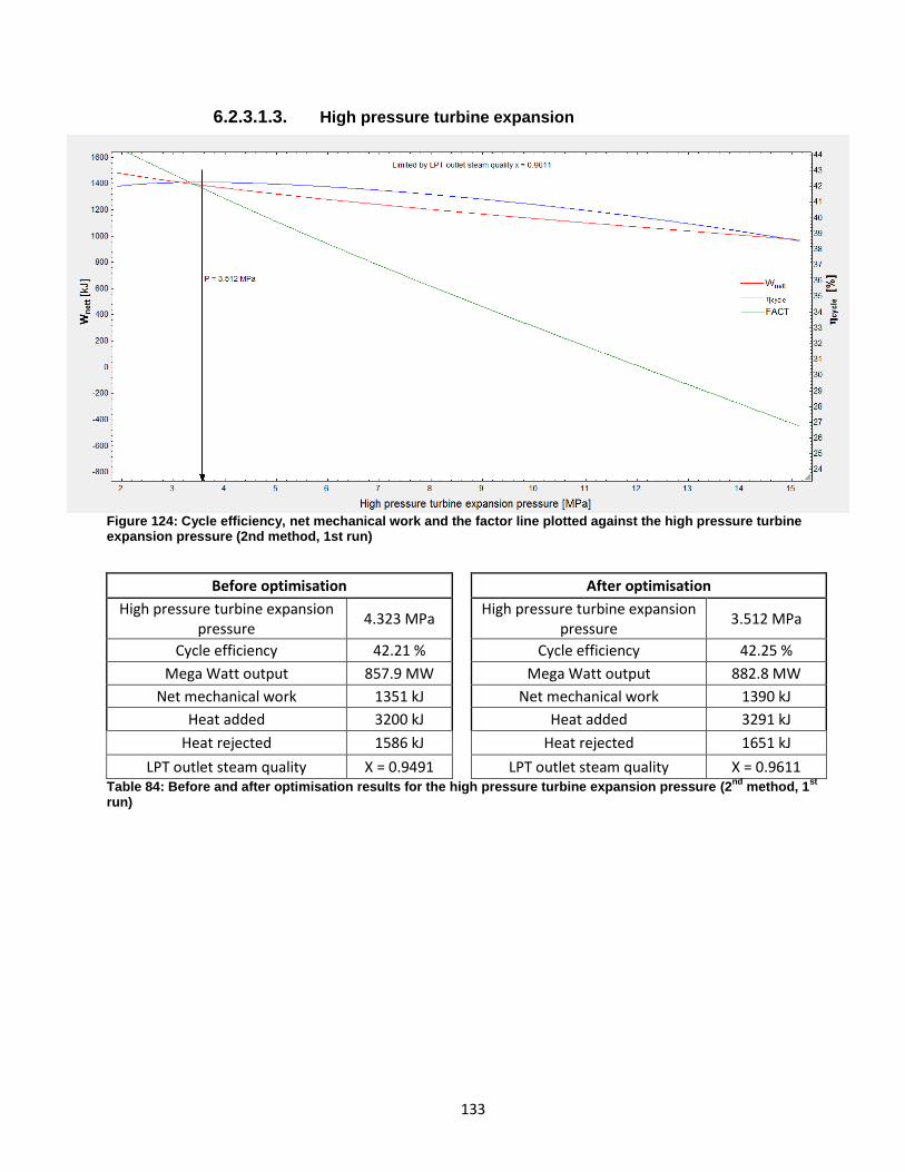
133
6.2.3.1.3. High pressure turbine expansion
Figure 124: Cycle efficiency, net mechanical work and the factor line plotted against the high pressure turbine expansion pressure (2nd method, 1st run)
Before optimisation
After optimisation
High pressure turbine expansion pressure
4.323 MPa
High pressure turbine expansion pressure
3.512 MPa
Cycle efficiency 42.21 %
Cycle efficiency 42.25 %
Mega Watt output 857.9 MW
Mega Watt output 882.8 MW
Net mechanical work 1351 kJ
Net mechanical work 1390 kJ
Heat added 3200 kJ
Heat added 3291 kJ
Heat rejected 1586 kJ
Heat rejected 1651 kJ
LPT outlet steam quality X = 0.9491 LPT outlet steam quality X = 0.9611 Table 84: Before and after optimisation results for the high pressure turbine expansion pressure (2
nd method, 1
st
run)

134
6.2.3.1.4. Low pressure heater 1
Figure 125: Cycle efficiency, net mechanical work and the factor line plotted against low pressure heater 1 steam bled off pressure (2nd method, 1st run)
Before optimisation
After optimisation
Low pressure heater 1 steam tap off pressure
0.05787 MPa
Low pressure heater 1 steam tap off pressure
0.05787 MPa
Cycle efficiency 42.25 %
Cycle efficiency 42.25 %
Mega Watt output 882.8 MW
Mega Watt output 882.8 MW
Net mechanical work 1390 kJ
Net mechanical work 1390 kJ
Heat added 3291 kJ
Heat added 3291 kJ
Heat rejected 1651 kJ
Heat rejected 1651 kJ Table 85: Before and after optimisation results for low pressure heater 1 steam tap off pressure (2
nd method, 1
st
run)

135
6.2.3.1.5. Low pressure heater 2
Figure 126: Cycle efficiency, net mechanical work and the factor line plotted against low pressure heater 2 steam bled off pressure (2nd method, 1st run)
Before optimisation
After optimisation
Low pressure heater 2 steam tap off pressure
0.1709 MPa
Low pressure heater 2 steam tap off pressure
0.2531 MPa
Cycle efficiency 42.25 %
Cycle efficiency 42.55 %
Mega Watt output 882.8 MW
Mega Watt output 889 MW
Net mechanical work 1390 kJ
Net mechanical work 1390 kJ
Heat added 3291 kJ
Heat added 3291 kJ
Heat rejected 1651 kJ
Heat rejected 1651 kJ Table 86: Before and after optimisation results for low pressure heater 2 steam tap off pressure (2
nd method, 1
st
run)

136
6.2.3.1.6. Low pressure heater 3
Figure 127: Cycle efficiency, net mechanical work and the factor line plotted against low pressure heater 3 steam bled off pressure (1st method, 1st run)
Before optimisation
After optimisation
Low pressure heater 3 steam tap off pressure
0.378 MPa
Low pressure heater 3 steam tap off pressure
0.3779 MPa
Cycle efficiency 42.55 %
Cycle efficiency 42.55 %
Mega Watt output 889 MW
Mega Watt output 889 MW
Net mechanical work 1390 kJ
Net mechanical work 1400 kJ
Heat added 3291 kJ
Heat added 3291 kJ
Heat rejected 1651 kJ
Heat rejected 1653 kJ Table 87: Before and after optimisation results for low pressure heater 3 steam tap off pressure (2
nd method, 1
st
run)

137
6.2.3.1.7. De-aerator
Figure 128: Cycle efficiency, net mechanical work and the factor line plotted against the de-aerator steam bled off pressure (2nd method, 1st run)
Before optimisation
After optimisation
De-aerator steam bled off pressure
0.7161 MPa
De-aerator steam bled off pressure
2.16 MPa
Cycle efficiency 42.55 %
Cycle efficiency 45.69 %
Mega Watt output 889 MW
Mega Watt output 889.3 MW
Net mechanical work 1400 kJ
Net mechanical work 1400 kJ
Heat added 3291 kJ
Heat added 3065 kJ
Heat rejected 1653 kJ
Heat rejected 1655 kJ Table 88: Before and after optimisation results for the de-aerator steam tap off pressure (2
nd method, 1
st run)

138
6.2.3.2. Second run
6.2.3.2.1. Boiler feed pump pressure
Figure 129: Cycle efficiency, net mechanical work and the factor line plotted against boiler feed pump discharge pressure (2nd method, 2nd run)
Figure 130: Cycle efficiency, net mechanical work and the factor line plotted against boiler feed pump discharge pressure (zoomed in) (2nd method, 2nd run)

139
Before optimisation
After optimisation
Boiler feed pump pressure 23.6 MPa
Boiler feed pump pressure 31.46 MPa
Cycle efficiency 45.69 %
Cycle efficiency 46.79 %
Mega Watt output 889.3 MW
Mega Watt output 875.3.3 MW
Net mechanical work 1400 kJ
Net mechanical work 1378 kJ
Heat added 3065 kJ
Heat added 2946 kJ
Heat rejected 1655 kJ
Heat rejected 1565 kJ Table 89: Before and after optimisation results for the boiler feed pump discharge (2
nd method, 2
nd run)
6.2.3.2.2. High pressure heater 6
Figure 131: Cycle efficiency, net mechanical work and the factor line plotted against the high pressure heater 6 steam tap off pressure (2nd method, 2nd run)
Before optimisation
After optimisation
High pressure heater 6 steam bled off pressure
2.865 MPa
High pressure heater 6 steam bled off pressure
2.865 MPa
Cycle efficiency 46.79 %
Cycle efficiency 46.79 %
Mega Watt output 875.3 MW
Mega Watt output 875.3 MW
Net mechanical work 1378 kJ
Net mechanical work 1378 kJ
Heat added 2946 kJ
Heat added 2946 kJ
Heat rejected 1565 kJ
Heat rejected 1565 kJ Table 90: Before and after optimisation results for high pressure heater 6 steam tap off pressure (2
nd method, 2
nd
run)
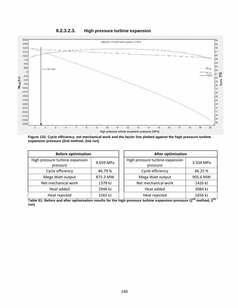
140
6.2.3.2.3. High pressure turbine expansion
Figure 132: Cycle efficiency, net mechanical work and the factor line plotted against the high pressure turbine expansion pressure (2nd method, 2nd run)
Before optimisation
After optimisation
High pressure turbine expansion pressure
4.659 MPa
High pressure turbine expansion pressure
3.504 MPa
Cycle efficiency 46.79 %
Cycle efficiency 46.25 %
Mega Watt output 875.3 MW
Mega Watt output 905.6 MW
Net mechanical work 1378 kJ
Net mechanical work 1426 kJ
Heat added 2946 kJ
Heat added 3084 kJ
Heat rejected 1565 kJ
Heat rejected 1656 kJ Table 91: Before and after optimisation results for the high pressure turbine expansion pressure (2
nd method, 2
nd
run)

141
6.2.3.2.4. Low pressure heater 1
Figure 133: Cycle efficiency, net mechanical work and the factor line plotted against low pressure heater 1 steam bled off pressure (2nd method, 2nd run)
Before optimisation
After optimisation
Low pressure heater 1 steam tap off pressure
0.05788 MPa
Low pressure heater 1 steam tap off pressure
0.05788 MPa
Cycle efficiency 46.25 %
Cycle efficiency 46.25 %
Mega Watt output 905.6 MW
Mega Watt output 905.6 MW
Net mechanical work 1426 kJ
Net mechanical work 1426 kJ
Heat added 3084 kJ
Heat added 3084 kJ
Heat rejected 1656 kJ
Heat rejected 1656 kJ Table 92: Before and after optimisation results for low pressure heater 1 steam tap off pressure (2
nd method, 2
nd
run)
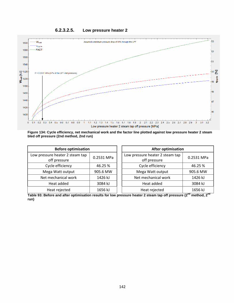
142
6.2.3.2.5. Low pressure heater 2
Figure 134: Cycle efficiency, net mechanical work and the factor line plotted against low pressure heater 2 steam bled off pressure (2nd method, 2nd run)
Before optimisation
After optimisation
Low pressure heater 2 steam tap off pressure
0.2531 MPa
Low pressure heater 2 steam tap off pressure
0.2531 MPa
Cycle efficiency 46.25 %
Cycle efficiency 46.25 %
Mega Watt output 905.6 MW
Mega Watt output 905.6 MW
Net mechanical work 1426 kJ
Net mechanical work 1426 kJ
Heat added 3084 kJ
Heat added 3084 kJ
Heat rejected 1656 kJ
Heat rejected 1656 kJ Table 93: Before and after optimisation results for low pressure heater 2 steam tap off pressure (2
nd method, 2
nd
run)

143
6.2.3.2.6. Low pressure heater 3
Figure 135: Cycle efficiency, net mechanical work and the factor line plotted against low pressure heater 3 steam bled off pressure (1st method, 2nd run)
Before optimisation
After optimisation
Low pressure heater 3 steam tap off pressure
0.3779 MPa
Low pressure heater 3 steam tap off pressure
0.3779 MPa
Cycle efficiency 46.25 %
Cycle efficiency 46.25 %
Mega Watt output 905.6 MW
Mega Watt output 905.6 MW
Net mechanical work 1426 kJ
Net mechanical work 1426 kJ
Heat added 3084 kJ
Heat added 3084 kJ
Heat rejected 1656 kJ
Heat rejected 1656 kJ Table 94: Before and after optimisation results for low pressure heater 3 steam tap off pressure (2
nd method, 2
nd
run)

144
6.2.3.2.7. De-aerator
Figure 136: Cycle efficiency, net mechanical work and the factor line plotted against the de-aerator steam bled off pressure (2nd method, 2nd run)
Before optimisation
After optimisation
De-aerator steam tap off pressure
2.16 MPa
De-aerator steam tap off pressure
2.16 MPa
Cycle efficiency 46.25 %
Cycle efficiency 46.25 %
Mega Watt output 905.6 MW
Mega Watt output 905.6 MW
Net mechanical work 1426 kJ
Net mechanical work 1426 kJ
Heat added 3084 kJ
Heat added 3084 kJ
Heat rejected 1656 kJ
Heat rejected 1656 kJ Table 95: Before and after optimisation results for the de-aerator steam tap off pressure (2
nd method, 2
nd run)

145
6.2.3.3. Third run
6.2.3.3.1. Boiler feed pump pressure
Figure 137: Cycle efficiency, net mechanical work and the factor line plotted against boiler feed pump discharge pressure (2nd method, 3rd run)
Figure 138: Cycle efficiency, net mechanical work and the factor line plotted against boiler feed pump discharge pressure (zoomed in) (2nd method, 3rd run)
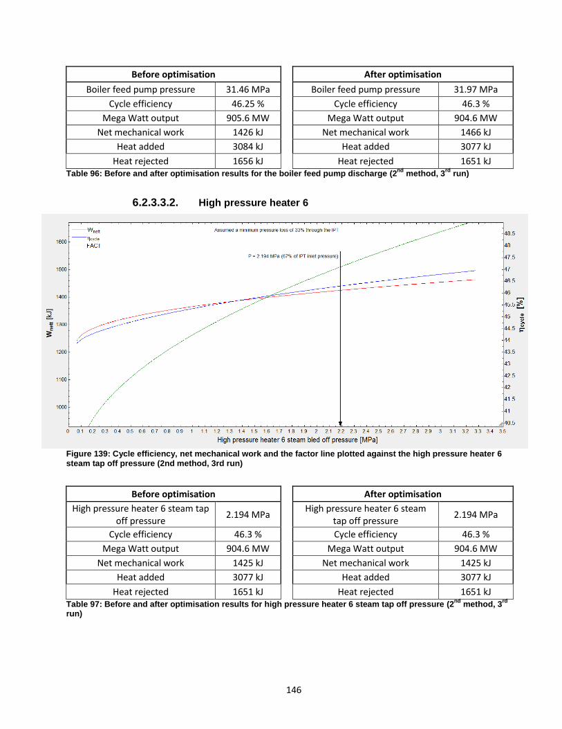
146
Before optimisation
After optimisation
Boiler feed pump pressure 31.46 MPa
Boiler feed pump pressure 31.97 MPa
Cycle efficiency 46.25 %
Cycle efficiency 46.3 %
Mega Watt output 905.6 MW
Mega Watt output 904.6 MW
Net mechanical work 1426 kJ
Net mechanical work 1466 kJ
Heat added 3084 kJ
Heat added 3077 kJ
Heat rejected 1656 kJ
Heat rejected 1651 kJ Table 96: Before and after optimisation results for the boiler feed pump discharge (2
nd method, 3
rd run)
6.2.3.3.2. High pressure heater 6
Figure 139: Cycle efficiency, net mechanical work and the factor line plotted against the high pressure heater 6 steam tap off pressure (2nd method, 3rd run)
Before optimisation
After optimisation
High pressure heater 6 steam tap off pressure
2.194 MPa
High pressure heater 6 steam tap off pressure
2.194 MPa
Cycle efficiency 46.3 %
Cycle efficiency 46.3 %
Mega Watt output 904.6 MW
Mega Watt output 904.6 MW
Net mechanical work 1425 kJ
Net mechanical work 1425 kJ
Heat added 3077 kJ
Heat added 3077 kJ
Heat rejected 1651 kJ
Heat rejected 1651 kJ Table 97: Before and after optimisation results for high pressure heater 6 steam tap off pressure (2
nd method, 3
rd
run)
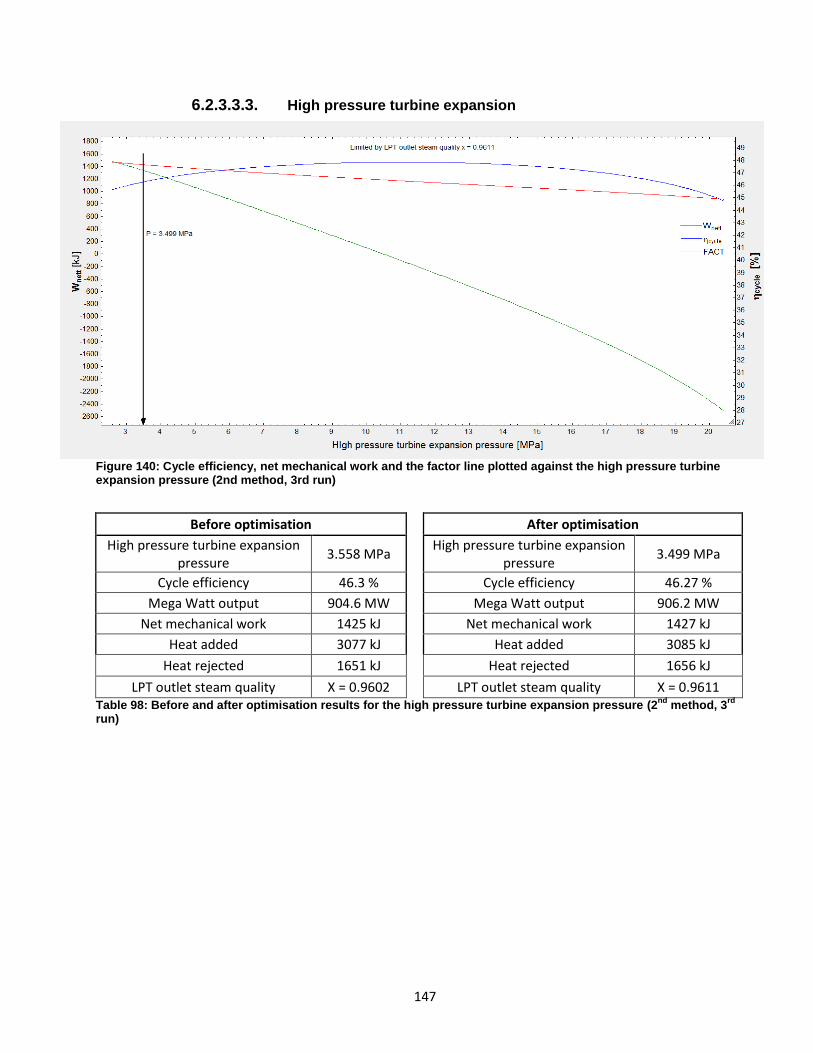
147
6.2.3.3.3. High pressure turbine expansion
Figure 140: Cycle efficiency, net mechanical work and the factor line plotted against the high pressure turbine expansion pressure (2nd method, 3rd run)
Before optimisation
After optimisation
High pressure turbine expansion pressure
3.558 MPa
High pressure turbine expansion pressure
3.499 MPa
Cycle efficiency 46.3 %
Cycle efficiency 46.27 %
Mega Watt output 904.6 MW
Mega Watt output 906.2 MW
Net mechanical work 1425 kJ
Net mechanical work 1427 kJ
Heat added 3077 kJ
Heat added 3085 kJ
Heat rejected 1651 kJ
Heat rejected 1656 kJ
LPT outlet steam quality X = 0.9602 LPT outlet steam quality X = 0.9611 Table 98: Before and after optimisation results for the high pressure turbine expansion pressure (2
nd method, 3
rd
run)
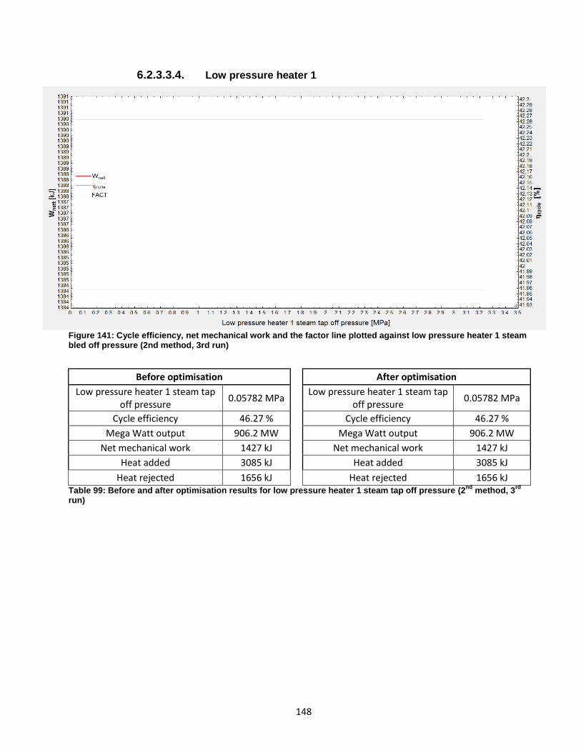
148
6.2.3.3.4. Low pressure heater 1
Figure 141: Cycle efficiency, net mechanical work and the factor line plotted against low pressure heater 1 steam bled off pressure (2nd method, 3rd run)
Before optimisation
After optimisation
Low pressure heater 1 steam tap off pressure
0.05782 MPa
Low pressure heater 1 steam tap off pressure
0.05782 MPa
Cycle efficiency 46.27 %
Cycle efficiency 46.27 %
Mega Watt output 906.2 MW
Mega Watt output 906.2 MW
Net mechanical work 1427 kJ
Net mechanical work 1427 kJ
Heat added 3085 kJ
Heat added 3085 kJ
Heat rejected 1656 kJ
Heat rejected 1656 kJ Table 99: Before and after optimisation results for low pressure heater 1 steam tap off pressure (2
nd method, 3
rd
run)

149
6.2.3.3.5. Low pressure heater 2
Figure 142: Cycle efficiency, net mechanical work and the factor line plotted against low pressure heater 2 steam bled off pressure (2nd method, 3rd run)
Before optimisation
After optimisation
Low pressure heater 2 steam tap off pressure
0.2529 MPa
Low pressure heater 2 steam tap off pressure
0.2529 MPa
Cycle efficiency 46.27 %
Cycle efficiency 46.27 %
Mega Watt output 906.2 MW
Mega Watt output 906.2 MW
Net mechanical work 1427 kJ
Net mechanical work 1427 kJ
Heat added 3085 kJ
Heat added 3085 kJ
Heat rejected 1656 kJ
Heat rejected 1656 kJ Table 100: Before and after optimisation results for low pressure heater 2 steam tap off pressure (2
nd method, 3
rd
run)

150
6.2.3.3.6. Low pressure heater 3
Figure 143: Cycle efficiency, net mechanical work and the factor line plotted against low pressure heater 3 steam bled off pressure (2nd method, 3rd run)
Before optimisation
After optimisation
Low pressure heater 3 steam tap off pressure
0.3775 MPa
Low pressure heater 3 steam tap off pressure
0.3775 MPa
Cycle efficiency 46.27 %
Cycle efficiency 46.27 %
Mega Watt output 906.2 MW
Mega Watt output 906.2 MW
Net mechanical work 1427 kJ
Net mechanical work 1427 kJ
Heat added 3085 kJ
Heat added 3085 kJ
Heat rejected 1656 kJ
Heat rejected 1656 kJ Table 101: Before and after optimisation results for low pressure heater 3 steam tap off pressure (2
nd method, 3
rd
run)
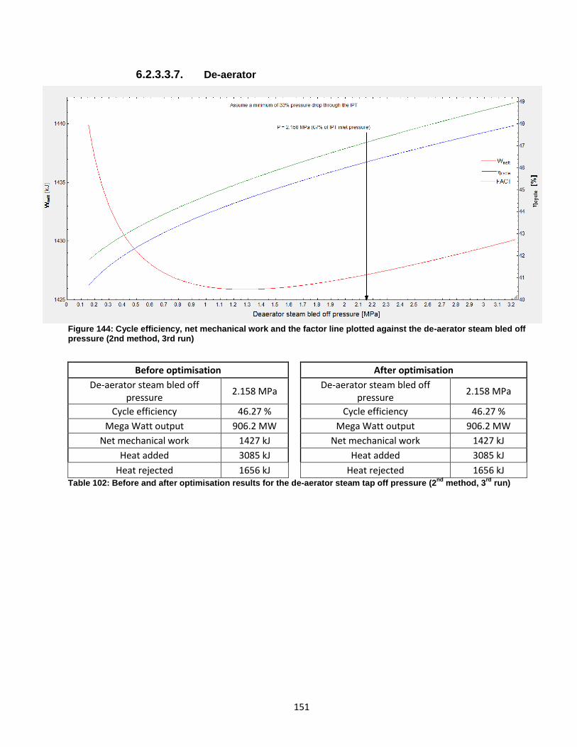
151
6.2.3.3.7. De-aerator
Figure 144: Cycle efficiency, net mechanical work and the factor line plotted against the de-aerator steam bled off pressure (2nd method, 3rd run)
Before optimisation
After optimisation
De-aerator steam bled off pressure
2.158 MPa
De-aerator steam bled off pressure
2.158 MPa
Cycle efficiency 46.27 %
Cycle efficiency 46.27 %
Mega Watt output 906.2 MW
Mega Watt output 906.2 MW
Net mechanical work 1427 kJ
Net mechanical work 1427 kJ
Heat added 3085 kJ
Heat added 3085 kJ
Heat rejected 1656 kJ
Heat rejected 1656 kJ Table 102: Before and after optimisation results for the de-aerator steam tap off pressure (2
nd method, 3
rd run)

152
6.2.3.3.8. Boiler feed pump pressure
Figure 145: Cycle efficiency, net mechanical work and the factor line plotted against boiler feed pump discharge pressure (2nd method, 4th run)
Figure 146: Cycle efficiency, net mechanical work and the factor line plotted against boiler feed pump discharge pressure (zoomed in) (2nd method, 4th run)
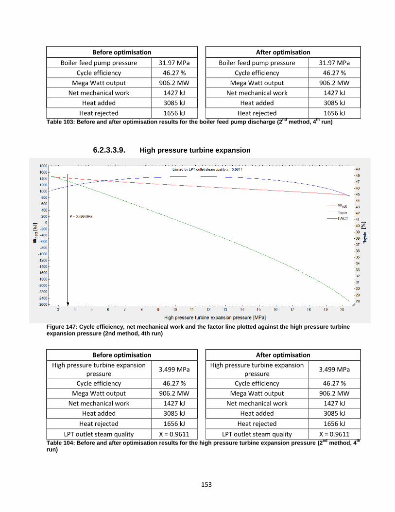
153
Before optimisation
After optimisation
Boiler feed pump pressure 31.97 MPa
Boiler feed pump pressure 31.97 MPa
Cycle efficiency 46.27 %
Cycle efficiency 46.27 %
Mega Watt output 906.2 MW
Mega Watt output 906.2 MW
Net mechanical work 1427 kJ
Net mechanical work 1427 kJ
Heat added 3085 kJ
Heat added 3085 kJ
Heat rejected 1656 kJ
Heat rejected 1656 kJ Table 103: Before and after optimisation results for the boiler feed pump discharge (2
nd method, 4
th run)
6.2.3.3.9. High pressure turbine expansion
Figure 147: Cycle efficiency, net mechanical work and the factor line plotted against the high pressure turbine expansion pressure (2nd method, 4th run)
Before optimisation
After optimisation
High pressure turbine expansion pressure
3.499 MPa
High pressure turbine expansion pressure
3.499 MPa
Cycle efficiency 46.27 %
Cycle efficiency 46.27 %
Mega Watt output 906.2 MW
Mega Watt output 906.2 MW
Net mechanical work 1427 kJ
Net mechanical work 1427 kJ
Heat added 3085 kJ
Heat added 3085 kJ
Heat rejected 1656 kJ
Heat rejected 1656 kJ
LPT outlet steam quality X = 0.9611 LPT outlet steam quality X = 0.9611 Table 104: Before and after optimisation results for the high pressure turbine expansion pressure (2
nd method, 4
th
run)
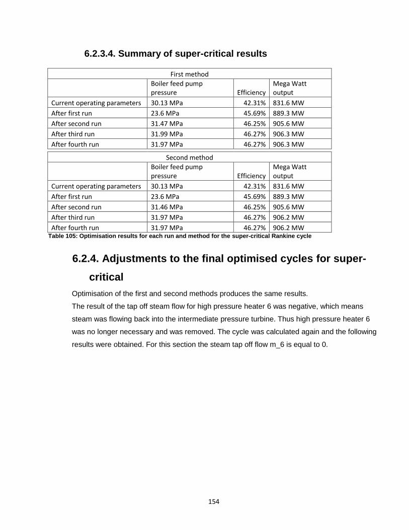
154
6.2.3.4. Summary of super-critical results
First method
Boiler feed pump pressure Efficiency
Mega Watt output
Current operating parameters 30.13 MPa 42.31% 831.6 MW
After first run 23.6 MPa 45.69% 889.3 MW
After second run 31.47 MPa 46.25% 905.6 MW
After third run 31.99 MPa 46.27% 906.3 MW
After fourth run 31.97 MPa 46.27% 906.3 MW
Second method
Boiler feed pump pressure Efficiency
Mega Watt output
Current operating parameters 30.13 MPa 42.31% 831.6 MW
After first run 23.6 MPa 45.69% 889.3 MW
After second run 31.46 MPa 46.25% 905.6 MW
After third run 31.97 MPa 46.27% 906.2 MW
After fourth run 31.97 MPa 46.27% 906.2 MW Table 105: Optimisation results for each run and method for the super-critical Rankine cycle
6.2.4. Adjustments to the final optimised cycles for super-
critical
Optimisation of the first and second methods produces the same results.
The result of the tap off steam flow for high pressure heater 6 was negative, which means
steam was flowing back into the intermediate pressure turbine. Thus high pressure heater 6
was no longer necessary and was removed. The cycle was calculated again and the following
results were obtained. For this section the steam tap off flow m_6 is equal to 0.

155
After high pressure heater 6 was taken out
Maximum boiler pressure 31.97 MPa
Cycle efficiency 46.53%
Mega Watt output 916.3 MW
Net mechanical work 1443 kJ
Heat added 3101 kJ
Heat rejected 1666 kJ Table 106: Results for super-critical cycle after optimisation and after high pressure heater 6 was taken out
Figure 148: Super-critical plant layout without high pressure heater 6

156
6.3. Sub-critical vs super-critical
6.3.1. Before optimisation
Sub-critical Super-critical
Feed pump 22.15 MPa 30.13 MPa
Maximum temperature 516°C 570°C
Minimum temperature 40°C 50°C
Maximum mass flow 415 kg/s 635 kg/s
Extraction pump discharge pressure 2.388 MPa 2.5 MPa
High pressure heater 6 bled steam tap off pressure 1.738 MPa 2.745 MPa
De-aerator bled steam tap off pressure 1.032 MPa 1.12 MPa
Low pressure heater 4 bled steam tap off pressure 0.4106 MPa
Low pressure heater 3 bled steam tap off pressure 0.1743 MPa 0.591 MPa
Low pressure heater 2 bled steam tap off pressure 0.06046 MPa 0.2671 MPa
Low pressure heater 1 bled steam tap off pressure 0.02991 MPa 0.09048 MPa
Cycle efficiency 42.69% 42.31%
Mega Watt out 538.4 MW 831.6 MW
Total work in 28.68 kJ 38.65 kJ
Total work out 1326 kJ 1348 kJ
Net mechanical work 1297 kJ 1310 kJ
Heat added 3039 kJ 3096 kJ
Heat rejected 1553 kJ 1495 kJ
Table 107: Comparison between sub- and super-critical Rankine cycles before optimisation
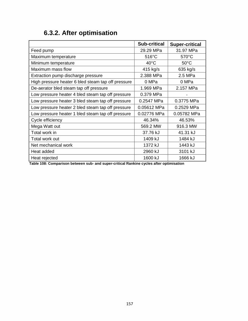
157
6.3.2. After optimisation
Sub-critical Super-critical
Feed pump 29.29 MPa 31.97 MPa
Maximum temperature 516°C 570°C
Minimum temperature 40°C 50°C
Maximum mass flow 415 kg/s 635 kg/s
Extraction pump discharge pressure 2.388 MPa 2.5 MPa
High pressure heater 6 bled steam tap off pressure 0 MPa 0 MPa
De-aerator bled steam tap off pressure 1.969 MPa 2.157 MPa
Low pressure heater 4 bled steam tap off pressure 0.379 MPa -
Low pressure heater 3 bled steam tap off pressure 0.2547 MPa 0.3775 MPa
Low pressure heater 2 bled steam tap off pressure 0.05612 MPa 0.2529 MPa
Low pressure heater 1 bled steam tap off pressure 0.02776 MPa 0.05782 MPa
Cycle efficiency 46.34% 46.53%
Mega Watt out 569.2 MW 916.3 MW
Total work in 37.76 kJ 41.31 kJ
Total work out 1409 kJ 1484 kJ
Net mechanical work 1372 kJ 1443 kJ
Heat added 2960 kJ 3101 kJ
Heat rejected 1600 kJ 1666 kJ
Table 108: Comparison between sub- and super-critical Rankine cycles after optimisation

158
7. Conclusion and recommendations
7.1. Conclusions In this study optimisation was used to optimise the boiler pressure, high pressure turbine
expansion and feed water heating steam tap of pressures.
The objective was to achieve higher efficiency and net mechanical work output with
optimisation. Optimisation allows us to find the optimal point to get the most efficiency without
losing too much net mechanical work.
After plotting the boiler feed pump optimised results the efficiency increased as the pressure
increased and the net mechanical work increased up to a certain pressure then started to
decrease. Thus finding an optimisation point was necessary to determine where the cycle
would benefit both.
After plotting the turbine expansion pressure optimised results it can be concluded that the
more the turbine expands the more efficiency and net mechanical work will be achieved.
Thus the limit on expansion is determined by the low pressure outlet steam quality. If the
steam quality exceeds the point where it transforms into liquid, more and bigger heat
exchangers will be needed as the volume of steam is much larger than liquid
After plotting the high pressure heater and the de-aerator optimised results it can be
concluded that the more tap off steam used the higher the efficiency and the net mechanical
work, but a minimum pressure loss through the intermediate turbine must be taken into
account.
After plotting the low pressure heater 4 (sub-critical) and low pressure heater 3 (super-critical)
it can be seen that as the steam tap off pressure from the intermediate pressure turbine
increases the efficiency and net mechanical work decrease. This is because the more energy
that is used for feed water heating the less energy is supplied to the intermediate turbine. The
minimum pressure is limited by the intermediate pressure turbine outlet pressure.
After plotting the optimised results for low pressure heater 3 (sub-critical) and low pressure
heater 2 (super-critical) it can be concluded that the more steam that is tapped off the higher

159
the efficiency and net mechanical work output achieved. This is because so little pressure is
used and more tap off pressure would result in an increase in efficiency and net mechanical
work. This is limited by a minimum pressure loss through the low pressure turbine.
After plotting the optimised results for low pressure heater 2 and low pressure heater 1 (sub-
critical) and low pressure heater 1 (super-critical) it can be concluded that the pressure is too
low to make a difference.
After looking at the whole cycle the conclusion can be drawn that when the maximum
temperature and pressure are raised the efficiency and net mechanical work rise as well. This
is limited by metallurgical conditions of the material that handles the temperature and
pressure. With better metallurgical conditions higher temperatures and pressure could be
achieved, thus super-critical and ultra-super-critical Rankine cycles are possible.
The main difference between these sub- and super-critical cycles is the limit of metallurgical
conditions. In the sub-critical cycle the temperature and pressure are limited and super-
critical cannot be achieved.
The pressure of the sub-critical and the super-critical cycles is almost the same after
optimisation. The reasons of the lower power generated output is because the mass flow of
the steam produced was not taken into account and kept constant for each cycle. Super-
critical cycles produce more mass flow of steam per second.
Temperature was also not taken into account and therefore the super-critical has a higher
temperature.
Steam tap off points are all dependent on the final temperature and pressure. With higher
temperature and pressure it is possible to tap off more steam and higher efficiencies could be
achieved.

160
However, the efficiency was increased by 3.65% on the sub-critical cycle and 4.22% on the
super-critical cycle with an increase of 30.8 MW and 84.7 MW respectively, the sub- and
super-critical cycles face major challenges before implementing the optimisation results on
the live plant.
The metallurgical conditions should be improved to handle the temperature and
pressure.
Bigger turbines are required for further and full expansion.
The steam tap off points need to be moved to accommodate the required pressure.
Bigger condensers are necessary if the final stage turbine does not expand fully.
This would cost a lot and is not economical to do on older plants, but for future use it can be
implemented in the design phase. If these results can be implemented it would save a lot of
money over time and lower emissions would result.
7.2. Recommendations The following recommendations can be made following the results achieved in the present study.
Ambient temperatures were not taken in account in this study, thus it can be
incorporated in future studies.
Cooling down the water returning from the cooling towers.
Simulating and optimising a Rankine cycle for ultra-super-critical boilers.
Programming the steam feed pump into the Rankine cycle and optimising it.
Optimising the maximum temperature for each cycle.
If this were to be implemented, it would be recommended to optimise one feed water
heater first to see how the cycle reacts before further optimisation is done.
Exploring possibilities with different materials to reach higher temperatures and
pressures.
161
8. References (BBE), Bureau of Energy Efficiency. 2004. Energy Efficiency Guide Book. Goverment of India.
(NISCO), Northern Industrial Supply Company. Products – Fans and Blowers. www.nisco.net/nyb.html
2009. ASHRAE Fundamentals Handbook.
An analysis of a thermal power plant working on a Rankine cycle : A theoretical
investigation. 2008. http://www.erc.uct.ac.za/jesa/volume19/19-1jesa-kapooria-etal.pdf Date of
access: 17 Mar 2015.
Aussie Tonic. http://igreenplanetstore.com/index.php?main_page=index&cPath=21 Date of
access: 11 April 2012.
BAHRAMI, M. Carnot cycle. Date of access: 12 Jun 2015.
<http://www.sfu.ca/~mbahrami/ENSC%20461/Notes/Carnot%20Cycle.pdf>
B-CUBED. 2014. LearnThermo. http://www.learnthermo.com/T1-tutorial/ch09/lesson-
B/pg08.php Date of access: 26 Aug 2015.
BLOWER), (Canadian. Industrial Fans and
Blowers. www.canadianblower.com/blowers/index.html Date of access: 8 April 2012.
Brazetek Heat Exchangers. http://www.brazetek.com/water-to-air-heat-exchangers Date of access:
11 April 2012.
BRITANNICA, The Editors of
Encyclopædia. Boiler. http://global.britannica.com/technology/boiler Date of access: 15 May 2013.
Buffaloblowers. http://buffaloblower.com/hvac/index.html
CHATTOPADHYAY, P. 2000. Boiler Operation Engineering. New Delhi: Tata McGraw-Hill Publishing
Company Limited.
COMPANY, The Babcock & Wilcox. 2005. Steam its generation and use.
COMPANY, FanAir. FanAir Company. www.fanair.com/products.pdf Date of access: 8 April 2012.
DOE), US Department of Energy (US. 1989. Energy Effieciency and Renewable
Energy. www1.eere.energy.gov/industry/bestpractices/pdfs/fan_sourcebook.pdf Date of access: 8
April 2012.
Electrical4u.com. 2015. http://www.electrical4u.com/rankine-cycle-efficiency-improvement-
techniques/ Date of access: 06 Sep 2015.

162
Engineering Teaching
Equipment. 2000/2005. http://www.discoverarmfield.co.uk/data/fm40/?js=enabled Date of access:
8 April 2012.
Engineering Toolbox. http://www.engineeringtoolbox.com/sizing-ducts-d_207.html Date of access:
9 April 2012.
GANASEAN. Fans, Pumps and Compressors. Indian Institute of tegnology.
GES. http://www.bowcott.com/ces/damper.htm Date of access: 11 April 2012.
HARSHAL D AKOLEKAR, P Srinivasan, Jagat Sesh Challa. 2014. Development of a Simulation Program
to Optimise Process Parameters of Steam Power Cycles. http://iasks.org/sites/default/files/7-1-
vol8.pdf Date of access: 2015 Nov 10.
HC Heat Exchangers. www.hcaircon.com
JOHNZACTRUBA. 2010. How are Supercritical Boilers different from Subcritical
Boilers? http://www.brighthubengineering.com/power-plants/32896-how-are-supercritical-boilers-
different-from-subcritical-boilers/ Date of access: 01 Nov 2015.
JOSEFSSON, Lars. 2014. LaMont steam boiler. http://www.steamesteem.com/?boilers/lamont-
boiler Date of access: 07 Feb 2014.
KUMAR, Ravindra, RAJU, Ramchandra & KUMAR, Ravi. 2013. Effect of Parameters in Once-Through
Boiler for Controlling Reheat Steam Temperature in Supercritical Power Plants. Research Jounal of
Engineering Sciences, 2(1):8. 01.
LAURE, Lizon-a-Lugarin. 2011. Publications. Date of access: 2 Nov 2015.
<https://publications.polymtl.ca/520/1/2011_LaureLizonALugrin.pdf>
LIMITED, Spirax Sarco. 2015. Water-tube
Boilers. http://www.spiraxsarco.com/Resources/Pages/Steam-Engineering-Tutorials/the-boiler-
house/water-tube-boilers.aspx Date of access: 02 Oct 2015.
LIRA, Carl. 2001 - 2013. Brief History of the Steam Engine. Date of access: 06 Jun 2013.
<http://www.egr.msu.edu/~lira/supp/steam/>
MACSTEEL. Pressure Vessel Steel 16Mo3. Date of access: 01 May 2015.
<http://www.macsteel.co.za/files/macsteel_vrn_-_pressure_vessel_steels_-_16mo3.pdf>
Made-in-china.com. http://polycore.en.made-in-china.com/offer/OfgEaPYMjnLm/Sell-Air-Flow-
Straightener.html Date of access: 11 April 2012.
MCGRAW-HILL. Handbook of Air Conditioning and Refrigeration.

163
MECHANICAL ENGINEERING. Lancashire Boiler. http://mechanical-engineering-
info.blogspot.co.za/2012/01/lancashire-boiler.html Date of access: 05 Jul 2013.
Mechanical. Engineering. http://mechanical-engineering-info.blogspot.com/2011/12/diesel-power-
plant.html Date of access: 04 Apr 2013.
NASA. National Aeronautics and space Administration. http://www.grc.nasa.gov/WWW/k-
12/airplane/pitot.html Date of access: 8 April 2012.
NUTZ, George. 1998. The forgotten Lamont Boiler. Date of access: 13 Aug 2013.
<https://www.steamautomobile.com/northea/lamont.html>
Power. http://www.powermag.com/jinzhushan-3-the-worlds-first-pc-fired-low-mass-flux-vertical-
tube-supercritical-boiler-part-2/ Date of access: 02 Oct 2015.
RAE, WH. 1984. Second Volume vols. Low-speed wind tunnel testing. New York: John Wiley & Sons,
Inc. 1 - 98 p.
RAJPUT, R.K. Thermal Engineering. New Delhi: Laxmi Publications.
RAYAPROLU, Kumar. 2009. BOILERS for POWER and PROCESS. New York: CRC Press (Taylor and
Francis Group).
SEBASTIAN TEIR. The History of Steam Generation. Date of access: 05 Jun 2013.
http://www.energy.kth.se/compedu/webcompedu/ManualCopy/Steam_Boiler_Technology/Basics_o
f_steam_generation/history_of_steam_generation.pdf
SHIMOGORI, Yoshio. 2012. APEC Energy Working Group. Date of access: 19 Jul 2013.
<http://www.egcfe.ewg.apec.org/publications/proceedings/CoalFlow/10thCFS-
11thCFET_2003/Session%2005/5-01Shimogori.pdf>
SIEMENS. 2006. Benson Once-Through Heat Recovery Steam Generator. Date of access: 03 Nov
2013. <http://www.energy.siemens.com/co/pool/hq/power-generation/power-plants/gas-fired-
power-plants/combined-cycle-powerplants/scc5-4000f-1s/A96001-S90-A496-X-4A00.pdf>
SIEMENS. 2006. Benson Once-Through Heat Recovery Steam Generators. Date of access: 05 Oct
2015. <http://www.energy.siemens.com/co/pool/hq/power-generation/power-plants/gas-fired-
power-plants/combined-cycle-powerplants/scc5-4000f-1s/A96001-S90-A496-X-4A00.pdf>
SIEMENS. 2009. BENSON Boiler Technology. Date of access: 15 Aug 2013.
http://www.energy.siemens.com/co/pool/hq/power-generation/power-plants/steam-power-plant-
solutions/BENSON-Boiler-Technology.pdf
STEINHAGEN, Muller & GOTTFRIED, Hans Micheal. 2011. Rankine
Cycle. http://www.thermopedia.com/content/1072/ Date of access: 07 Mar 2014.

164
Supercritical Boilers. In: Supercritical Boilers, Baboo Ram. 1-98 p.
TEIR, Sebastian & KULLA, Antto. 2002. Natural circulation boilers. In: Steam/Water Circulation
Design, Espoo, Finland: Helsinki University of Technology. 22 p.
The Stirling Boiler. Date of access: 05 Oct 2013.
<http://www.asope.org/pdfs/The_Stirling_Boiler%5b1%5d.pdf>
Thermodynamics Manual / B-Tech Mechanical / Babcock & Wilcox
Boiler. 2014. http://www.mechanicalhero.com/2011/12/thermodynamics-manual-b-tech-
mechanical.html Date of access: 20 Jan 2014.
Thermodynamics Manual. http://sumitshrivastva.blogspot.com/2011/12/thermodynamics-manual-
b-tech-mech_20.html Date of access: 05 Apr 2013.
THERMOPEDIA. 2011. http://www.thermopedia.com/content/1072/ Date of access: 28 Sep 2015.
Ultra Super Critical Pressure Coal Fired
Boiler. http://www.egcfe.ewg.apec.org/publications/proceedings/CoalFlow/10thCFS-
11thCFET_2003/Session%2005/5-01Shimogori.pdf
University of Cambridge. http://www.ceb.cam.ac.uk/pages/hydrodynamic-voltammetry.html Date
of access: 11 April 2012.

165
9. Appendix
9.1. Appendix A
9.1.1. Material development
Figure 149: Kriel power station (sub-critical) boiler material

166
Figure 150: Medupi power station (super-critical) boiler material
The challenge was to develop material that can handle the intense heat and enormous pressure. P91
was developed (with 9% chromium) for the final stages of the superheat and reheat where the
temperature is above 540°C. The new super-critical boilers use 13CrMo45 (with 1% chromium)
material for the water walls (evaporation stage). 13CrMo45 was previously used in sub-critical boilers
and performs outstandingly.
16Mo3 is used in the economiser. 16Mo3 is a chrome molybdenum steel alloy that is perfect for heat
and corrosion resistance and is wear and fatigue resistant. 16Mo3 has a good tensile and yield
strength with great toughness.
Reheater 1 is made up of four stages. The inlet and first sections are P235 GH. The second section is
16Mo3. The third section is 13CrMo45 with the outlet section as 10CrMo910.
The Superheater 2 is made up of VM12SHC.
The Reheater 2 and Superheater 3 are made up of TP347HFG.

167
Superheater 1 is made of 7CrMoVTi10-10.
Superheater 2, Reheater 2 and Superheater 3 inlet and outlet sections are made up of T91 material.
168
9.2. Appendix B
9.2.1. Sub-critical boilers
9.2.1.1. Introduction
Mark Benson wanted to generate steam with no pressure limit and in 1922 the once-
through Benson boiler was born. In the mid-twenties Siemens took over and developed
the Benson boiler further. Siemens recognised that a once-through evaporator could
be used for sub-critical as well as super-critical boilers. Once-through boilers used
smaller diameter tubes with a thinner wall thickness which promoted heat transfer
more quickly and resulted in more steam produced in an hour.
Natural circulation is sacrificed in order to increase the boiler size and efficiency.
The once-through Benson boiler uses the spiral configuration for the evaporation walls.
This ensures a higher steam quality with lower temperatures because it transfers heat
better with an incline of 15 degrees.
The feed water pump is used to create force circulation of the water through the boiler.
9.2.1.2. Advantages of a sub-critical cycle
High overall efficiency even at part loads.
Can be used in a pressure range of 10 – 35 MPa without modifying the evaporator
Short start-up time
Suitable for all coal grades.
Economical
Low-stress operation
Flexible operating modes
169
9.2.2. Super-critical boilers
9.2.2.1. Introduction
After the Second World War there was rapid economic development. The need for a
more efficient and economical power plant was on the increase. This would mean that
there had to be an improvement in material metallurgy and water chemistry as well as
combustion to make operations at super-critical pressures possible.
The critical pressure for water is 22.06 MPa. Above 22.06 MPa there is no two phase
stage (water and steam).
9.2.2.2. Cycle
This cycle is based on a boiler that is on load and has passed the start-up phase.
Demineralised water is pumped into the boiler economiser. At the economiser exit the
water makes its way down and enters the spiral wall where it transforms halfway up
into a vertical wall; the water and steam mixture accumulates again at the top outlet
headers. The water and steam mixture is split into four separating vessels where the
steam and water separate. The separated water accumulates in the collecting vessel
(only during start-up) and is fed to the economiser again where the steam enters
superheater 1 then superheater 2 and then superheater 3. After superheater 3 the
steam condition is superheated steam and is ready for the high pressure turbine. The
steam is sent to the high pressure turbine where it transforms into mechanical work.
After the high pressure turbine the steam loses a lot of energy and is sent back to the
boiler where it enters Reheater 1 and then Reheater 2 to turn it again into superheated
steam. The steam is now ready for the intermediate pressure turbine and the low
pressure turbine.
After the low pressure turbine the water and steam mixture goes through the
condenser where heat transfer takes place and the energy is extracted out of the water
to transform it into a liquid again. The water is pumped through the low pressure
heaters that use tap off steam from the intermediate and low pressure turbines to
increase the water temperature before it enters the de-aerator. More heat transfer

170
takes place in the de-aerator with tap off steam from the intermediate turbine to
increase the temperature of the water. The de-aerator serves as an inlet for the boiler
feed pump, where the water is pumped through the high pressure heaters that use tap
off steam from the high pressure turbine exit and intermediate turbine for more heat
exchange before it enters the economise to start the cycle again.
9.2.2.3. Advantages
High plant efficiency, high efficiency coal utilisation, low emission (CO2)
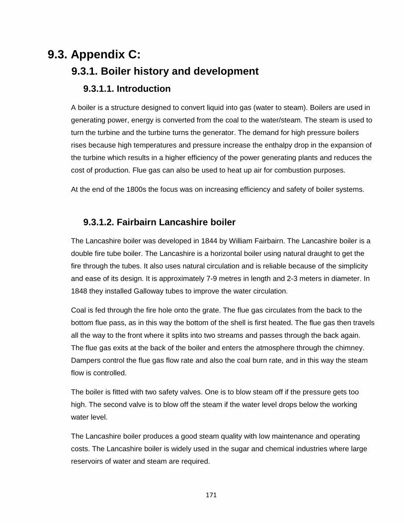
171
9.3. Appendix C:
9.3.1. Boiler history and development
9.3.1.1. Introduction
A boiler is a structure designed to convert liquid into gas (water to steam). Boilers are used in
generating power, energy is converted from the coal to the water/steam. The steam is used to
turn the turbine and the turbine turns the generator. The demand for high pressure boilers
rises because high temperatures and pressure increase the enthalpy drop in the expansion of
the turbine which results in a higher efficiency of the power generating plants and reduces the
cost of production. Flue gas can also be used to heat up air for combustion purposes.
At the end of the 1800s the focus was on increasing efficiency and safety of boiler systems.
9.3.1.2. Fairbairn Lancashire boiler
The Lancashire boiler was developed in 1844 by William Fairbairn. The Lancashire boiler is a
double fire tube boiler. The Lancashire is a horizontal boiler using natural draught to get the
fire through the tubes. It also uses natural circulation and is reliable because of the simplicity
and ease of its design. It is approximately 7-9 metres in length and 2-3 meters in diameter. In
1848 they installed Galloway tubes to improve the water circulation.
Coal is fed through the fire hole onto the grate. The flue gas circulates from the back to the
bottom flue pass, as in this way the bottom of the shell is first heated. The flue gas then travels
all the way to the front where it splits into two streams and passes through the back again.
The flue gas exits at the back of the boiler and enters the atmosphere through the chimney.
Dampers control the flue gas flow rate and also the coal burn rate, and in this way the steam
flow is controlled.
The boiler is fitted with two safety valves. One is to blow steam off if the pressure gets too
high. The second valve is to blow off the steam if the water level drops below the working
water level.
The Lancashire boiler produces a good steam quality with low maintenance and operating
costs. The Lancashire boiler is widely used in the sugar and chemical industries where large
reservoirs of water and steam are required.
172
The boiler has steel rings that are welded or riveted to form two parallel cylindrical shells that
run through the boiler and carry the hot flue gas. The flue gas cylindrical shells lie below the
water level to accommodate a grate of sufficient area with minimum length. The flue gas
cylindrical shells are larger in diameter at the front and this helps with the control of gas flow
and the amount of air entering the grate.
The Lancashire boiler uses about six tons of coal per day (about 250kg/h or 0.0694kg/s).
9.3.1.3. Babcock and Wilcox boiler
The Wilcox boiler was developed in 1867 by George Herman Babcock and Stephan Wilcox.
This water tube boiler has a larger heating area and allows a much better water circulation
which creates a much safer boiler. The tubes are placed in the furnace area at about 10 – 15
degrees angle which promotes water circulation. These tubes are heated by the flue gas
radiation and convection. Steam is collected in a drum situated above the tubes. This drum
contains water and steam with a safety valve.
The boiler is situated horizontally and is only filled halfway with water. The header is
connected with tubes that are in a zig zag configuration in the combustion chamber as flue
gas passes over tubes to transfer heat. There is a tube that takes steam back to the
combustion chamber for more heating, thus becoming superheated steam. This boiler had a
much greater heat transfer and was more effective than previous boilers. The water tube
boilers became the standard for future boilers. With multiple tubes in the boiler and better
quality steel higher pressure and temperatures could be achieved. This has become the boiler
of choice for steam turbines. The tubes are tilled 5 – 15 degrees to achieve a natural
water/steam flow. There are two baffles to deflect the hot flue gases. The boiler has a mud
box that is situated at the end of the down comer. The mud box collects any impurities and
mud that are found in the water A blow off cock is used to get rid of the impurities in the mud
box.
9.3.1.3.1. Operating method
Coal is fed onto the grate through the fire doors. The coal is burned and the flue gas rises
upwards. The baffle box redirects the flue gas and travels in a zig-zag manner to cover as
much as possible of the tube area. The flue gas exits the boiler and enters the
atmosphere through the chimney.

173
The boiler makes use of natural circulation. The water in the drum travels down to the
bottom into the tubes and is heated. The water turns into steam and the density
decreases, which results in more steam in the drum. The steam is returned to the furnace
through tubes known as the superheater. The superheater increases the temperature of
the steam and becomes superheated.
There is a damper fitted on the flue gas outlet. This controls the burn rate and load of
steam produced.
9.3.1.3.2. Advantages
Higher steam pressures, resulting in higher cycle efficiency.
Easy repairable and all components can be inspected.
Can expand and contact freely.
Hot gases flow at the same angle as the water, thus resulting in a maximum heat
transfer.
Tubes are angled at 10 - 15 degrees, resulting in better water circulation.
9.3.1.3.3. Disadvantages
Not suitable for water with a lot of impurities and mud, as these easily form blockages
and result in short term overheating of tubes. The tubes burst and cause a lot of
damage.
Higher maintenance cost.
Water levels must be watched, and a failure in the power supply even for a small
period can result in the boiler overheating.
9.3.1.4. Stirling boiler
This boiler was designed by Alan Stirling and operated from 1883 to 1927. The first design
contains two upper drums and one lower drum (mud drum). The upper drums were connected
to the lower mud drum with slightly bent tubes to connect the periphery to the drum. This was
further developed and a fourth drum was added on top. This was known as a four drum boiler.
In 1906 the Babcock and Wilcox Company took over the Stirling boiler company. The three
drums are set on top in parallel and are connected to the mud drum below. The middle drum
is slightly higher than the front and rear drum. The top side of the middle drum is connected to
the front and rear drum for the steam so move freely into the middle drum. The middle and

174
rear drum bottom parts are connected to maintain the water level. The front drum is where
water enters and is fed to the tubes. All steam is collected at the middle drum. The safety
valve can also be located on the middle drum. There is a blow-off valve on the bottom of the
mud drum to get rid of impurities.
The boiler has a manhole in one end of each of the four drums. This makes it easy to enter
the boiler for inspection and repairs. The furnace is built out of bricks and has an arch-shaped
roof. This design made it possible to use almost any type of fuel. The baffle walls were built
from the mud drum to almost each top drum. These baffle walls prevent the flue gas from
passing straight through the furnace without going through all the tubes.
9.3.1.4.1. Operating method
Coal is fed onto the grating where it burns. The flue gas then rises to the top and with the
help of baffle plates is sucked down before it goes up again and leaves the furnace to exit
through a chimney into the atmosphere. Just before the flue gas exits the furnace there is
a control valve that controls the rate at which gas exits, and in this way the boiling rate
can be controlled as well as the amount of steam needed.
The three top drums are only half filled with water to separate the water and steam. The
drums are connected to each other at the top, while the right hand top drum and middle
top drum are connected to maintain the water level. The left drum is where the water is
added to the system. There is also a drum at the bottom that is called the mud drum. The
mud drum is there to collect mud and impurities and then let it drain out. A blow of valves
is situated on top to blow off impurities in the water.
If a superheater is needed, it would be fitted between the right hand side top drum and
middle top drum where the flue gas is still very hot.
9.3.1.4.2. Advantages
Easy load changes because of the small water contend.
Tube and drum dimensions made it possible for high steam pressures (160 bar)
Design made it possible for any burner arrangement - horizontal or vertical.
Full control of temperature.
Free to expand
Can handle water with impurities better

175
9.3.1.4.3. Disadvantages
More difficult to manufacture
Limited steam amounts produced.
9.3.1.5. Tube walled furnace
The demand for more steam increased rapidly because more power needed to be generated.
This would require a larger furnace, which led to the development of the tube walled furnace.
With this design the combustion and heat transfer areas are in the same place. This means
more savings in construction costs and a massive increase in boiler size. In 1955 the first fully
tube welded furnace was constructed. With a tube walled boiler the heat is transferred through
radiation in the combustion process.
9.3.1.6. La Mont boiler
9.3.1.6.1. Introduction
The La Mont boiler is a once through boiler with lots of small diameter tubes running from
bottom to top in a helical configuration. The tubes are spaced with a little spacing between
them. The La Mont boiler uses forced circulation for the water and therefore requires
powerful pumps.
The La Mont boiler was the first forced circulation boiler introduced by La Mont in 1925
and was used in America and Europe. This was the first high pressure steam boiler. The
La Mont concept was safer, lighter and more effective. This boiler was also used in World
War 2 navy ships.
The La Mont Boiler consists of a feed pump to force water through the boiler. The water
is pumped through the economiser and then enters the steam drum. The circulating pump
was used to pump the water from the steam drum into the vertical wall tubes that are
used as the first part of evaporation.
The boiler makes use of helical coil tubes from top to bottom. A little steam drum was
used to separate steam and water. The water was fed back into the boiler with a
circulation pump.

176
9.3.1.6.2. Operating method
The La Mont boiler is a once through boiler. Air is sucked through the boiler to extract hot
flue gases. The flue gases pass through the furnace and transfer heat to the tubes.
Helical configuration is used for the tubes to maximise the heat transfer. The gas passes
from bottom to the top and then exits the boiler. Later the air heater was introduced and
the gas would pass through the air heater to transfer heat to be used for combustion. This
heat was transferred without mixing clean air with flue gas. This resulted in better
combustion.
The La Mont boiler consists of an economiser, superheater and a set of convection tubes.
The feed water is pumped into the economiser which is situated at the top of the boiler.
The water enters the separating drum where the water and steam separate. The water is
pumped through the water walls where it is exposed to radiant heat transfer; it then enters
the convection tube area where it is exposed to convection heat transfer. At the end of the
convection element it is all steam and enters the separating drum. The steam enters the
superheater circuit where it absorbs more heat and becomes super-heated steam.
The La Mont uses fuel oil, crushed coal or gas as heat source.
9.3.1.6.2.1. Air circuit
A blower is used to blow cold air through the air heater to transfer heat for combustion
secondary air. The air heater receives heat from the flue gas exiting the boiler.
9.3.1.6.2.2. Water circuit
The circuit starts with a de-aerator; water is pumped from the de-aerator into the
economiser which acts as a heat exchanger. The vapour water mix is separated with
the help of a separating drum. The remaining water in the separating drum is fed into a
circulating pump to pump it through a primary and secondary evaporating coils system
to return it to the steam drum.
9.3.1.6.2.3. Steam circuit
The separated steam in the drum is then fed through the superheater for more heat
transfer and higher temperatures are achieved. The steam is then fed to the turbine.

177
9.3.1.6.3. Advantages
Uses forced circulation, which helps with a positive circulation and evaporation.
There are high heat transfer rates because of small diameter tubes, thus more steam
is produced per hour
Low carbon tubes were available, resulting in a safer boiler
There is a short start-up time, thus it is perfect for peak times.
9.3.1.6.4. Disadvantages
It requires a small vertical drum outside with a small circulation pump.
There is a limited amount of steam
Temperature and pressure are limited because of metallurgical conditions