evaluation of regional slamm results to establish a...
TRANSCRIPT

Evaluation of Regional SLAMM Results to Establish a Consistent Framework of Data and
Models
Gulf Coast Prairie Land Conservation Cooperative
December 15, 2014
PO Box 315, Waitsfield VT, 05673 (802)-496-3476

Warren Pinnacle Consulting, Inc. 2
Evaluation of Regional SLAMM Results to Establish a Consistent Framework of Data and Models
Background ................................................................................................................................................... 4
Model Summary ........................................................................................................................................ 5
SLAMM Application Methods ....................................................................................................................... 7
Study Area ................................................................................................................................................. 7
Model Time steps ...................................................................................................................................... 8
Sea Level Rise Scenarios ............................................................................................................................ 8
Gap Study Area Input Raster Preparation ................................................................................................. 8
Elevation Data ....................................................................................................................................... 8
Slope Layer ............................................................................................................................................ 8
Elevation correction .............................................................................................................................. 8
Wetland Layers and translation to SLAMM wetland categories .......................................................... 9
Dikes and Impoundments ..................................................................................................................... 9
Percent Impervious ............................................................................................................................... 9
Gap Study Areas Parameterization ......................................................................................................... 10
Erosion Rates ...................................................................................................................................... 10
Historic sea level rise rates ................................................................................................................. 11
Tide Ranges ......................................................................................................................................... 11
Salt Elevation ....................................................................................................................................... 11
Accretion Rates ....................................................................................................................................... 12
Model Calibration ................................................................................................................................... 19
Elevation Pre-processor .......................................................................................................................... 20
Freshwater Flow Polygons ...................................................................................................................... 21
Flooded Swamp ....................................................................................................................................... 21
Considerations for individual study areas ............................................................................................... 22
Study Area 1 – South Florida ............................................................................................................... 24
Study Area 2 – South Florida ............................................................................................................... 24
Study Area 3 – Florida ......................................................................................................................... 24
Study Area 4 – Florida ......................................................................................................................... 24
Study Area 5 – Lake Rousseau, Florida ............................................................................................... 24

Warren Pinnacle Consulting, Inc. 3
Study Area 6 – Florida ......................................................................................................................... 25
Study Area 7 – Florida ......................................................................................................................... 25
Study Area 8 – Florida ......................................................................................................................... 25
Study Area 9 – St. Joe Bay and Carabelle, Florida ............................................................................... 25
Study Area 10 – Florida ....................................................................................................................... 25
Study Areas 11 and 13 - Florida .......................................................................................................... 25
Study Area 12 – Alabama .................................................................................................................... 25
Study Area 14 – Mississippi and Louisiana .......................................................................................... 25
Study Area 16 – Dry Tortugas, Florida ................................................................................................ 26
Study Area 17 – Louisiana Chenier Plain ............................................................................................. 26
Study Area 18 – Galveston Bay, Texas ................................................................................................ 26
Study Area 19 – Matagorda and San Antonio Bays, Texas ................................................................. 26
Study Area 20 – Baffin Bay, South Texas ............................................................................................ 26
Study Area 21 – Florida ....................................................................................................................... 27
Focal Species Approach .......................................................................................................................... 27
Results and Discussion ................................................................................................................................ 29
Conclusions and Perspectives ..................................................................................................................... 43
References .................................................................................................................................................. 44
Appendix A ................................................................................................................................................ A-1
Appendix B ................................................................................................................................................. B-1
Appendix C ................................................................................................................................................. C-1
Warren Pinnacle Consulting, Inc. 4
Background
From 2008 to 2013 the Sea Level Affecting Marshes Model (SLAMM) was applied to more than ten million hectares of the Gulf of Mexico coastline. However, simulation results were not directly comparable due to differences in model domain definitions, accretion modeling approaches, and future sea-level scenarios. In addition, several gap areas had not yet been modeled. In 2014, the Gulf Coast Prairie Land Conservation Cooperative funded this analysis of the US Gulf of Mexico Coast.in order to establish a consistent framework of data and models. The main objectives of this project were to generate a seamless set of landcover projections for the Gulf of Mexico coast using SLAMM and conduct a focal species analysis using SLAMM results. Additional project goals included deriving and applying mechanistic accretion feedbacks for coastal marshes, analysis of the effects of low-quality (non-LiDAR) elevation data on model results, and posting the SLAMM outputs to SLAMM-View (www.slammview.org) for public access to results.
The study area (Figure 1) includes coastline in the Gulf Coast Prairie, South Atlantic, Gulf Coast Plains and Ozarks, and Peninsular Florida Landscape Conservation Cooperatives. Results of the study will provide a gulf-wide dataset to help identify the most appropriate adaptation strategies for specific areas including land acquisition, marsh restoration, infrastructure development, and other land and facility management actions.
Tidal marshes are dynamic ecosystems that provide significant ecological and economic value. Given that tidal marshes are located at the interface between land and water, they can be among the most susceptible ecosystems to climate change, especially accelerated sea-level rise (SLR). Numerous factors can affect marsh fate including the elevation of marshes relative to the tides, marshes’ frequency of inundation, the salinity of flooding waters, the biomass of marsh platforms, land subsidence, marsh substrate, and the settling of suspended sediment into the marshes. Because of these factors, a simple calculation of current marsh elevations as compared to future projections of sea level does not provide an adequate estimation of wetland vulnerability.
Changes in tidal marsh area and habitat type in response to sea-level rise were modeled using the Sea Level Affecting Marshes Model (SLAMM 6). SLAMM is widely recognized as an effective model to study and predict wetland response to long-term sea-level rise (Park et al. 1991) and has been applied in every coastal US state (Craft et al. 2009; Galbraith et al. 2002; Glick et al. 2007, 2011; National Wildlife Federation and Florida Wildlife Federation 2006; Park et al. 1993; Titus et al. 1991).

Warren Pinnacle Consulting, Inc. 5
Figure 1. Project Study Area
Model Summary
SLAMM predicts when marshes are likely to be vulnerable to SLR and where marshes may migrate upland in response to changes in water levels. The model attempts to simulate the dominant processes that affect shoreline modifications during long-term sea-level rise and uses a complex decision tree incorporating geometric and qualitative relationships to represent transfers among coastal classes. SLAMM is not a hydrodynamic model but long term shoreline and habitat changes are modeled as a succession of equilibrium states with sea level. Model outputs include map distributions of wetlands at different time steps in response to sea level rise changes as well as tabular and graphical data. The models relative simplicity and modest data requirements allow its application at a reasonable cost. Mcleod and coworkers wrote in their review of sea-level rise impact models that “... the SLAMM model provides useful, high-resolution, insights regarding how sea-level rise may impact coastal habitats” (Mcleod et al. 2010).
SLAMM assumes that wetlands inhabit a range of vertical elevations that is a function of the tide range. Elevation loss relative sea level is computed for each cell in each time step: it is given by the

Warren Pinnacle Consulting, Inc. 6
sum of the historic SLR eustatic trend, the site specific or cell specific rate of change of elevation due to subsidence and isostatic adjustment, and the accelerated sea level rise depending on the scenario considered. Sea level rise is offset by sedimentation and accretion.
When the model is applied, each study site is divided into cells of equal area that are treated individually. The conversion from one land cover class to another is computed by considering the new cell elevation at a given time step with respect to the class in that cell and its inundation frequency. Assumed wetland elevation ranges may be estimated as a function of tidal ranges or may be entered by the user if site-specific data are available. The connectivity module determines salt water paths under normal tidal conditions. In general, when a cell’s elevation falls below the minimum elevation of the current land cover class and is connected to open water, then the land cover is converted to a new class according to a decision tree.
In addition to the effects of inundation represented by the simple geometric model described above, the model can account for second order effects that may occur due to changes in the spatial relationships among the coastal elements. In particular, SLAMM can account for exposure to wave action and its erosion effects, overwash of barrier islands where beach migration and transport of sediments are estimated, saturation allowing coastal swamps and fresh marshes to migrate onto adjacent uplands as a response of the fresh water table to rising sea level close to the coast, and marsh accretion.
Marsh accretion is the process of wetland elevations changing due to the accumulation of organic and inorganic matter. Accretion is one of the most important processes affecting marsh capability to respond to SLR. The SLAMM model was one of the first landscape-scale models to incorporate the effects of vertical marsh accretion rates on predictions of marsh fates, including this process since the mid-1980s (Park et al. 1989). Since 2010, SLAMM has incorporated dynamic relationships between marsh types, marsh elevations, tide ranges, and predicted accretion rates. The SLAMM application presented here utilizes a mechanistic marsh accretion model to define relationships between tide ranges, water levels, and accretion rates (Morris 2013; Morris et al. 2002).
As with any numerical model, SLAMM has important limitations. As mentioned above, SLAMM is not a hydrodynamic model. Therefore, cell-by-cell water flows are not predicted as a function of topography, diffusion and advection. Furthermore, there are no feedback mechanisms between hydrodynamic and ecological systems. Solids in water are not accounted for via mass balance which may affect accretion (e.g. local bank sloughing does not affect nearby sedimentation rates). The erosion model is also very simple and does not capture more complicated processes such as “nick-point” channel development. A more detailed description of model processes, underlying assumptions, and equations can be found in the SLAMM 6.2 Technical Documentation (available at www.warrenpinnacle.com/prof/SLAMM).

Warren Pinnacle Consulting, Inc. 7
SLAMM Application Methods
Study Area
The United States coast of the Gulf of Mexico was modeled from Key West, FL to the Mexico border (Figure 1). This study area was comprised of 25 areas with existing SLAMM simulations (listed in Table 1) and 20 new ‘gap’ study areas.
Table 1. Existing SLAMM Study Areas Site Name State cell size Original project funder Mobile Bay AL 30 TNC-EPA St. Marks FL 10 USFWS Pensacola Bay FL 15 TNC-EPA Perdido Bay FL 30 TNC-EPA Southern Big Bend FL 30 TNC-EPA Tampa Bay FL 15 TNC-EPA Saint Andrew Choctawhatchee FL 10 TNC- GOMA Apalachicola FL 30 USFWS Great White Heron FL 10 GOMF Lower Suwannee FL 30 USFWS 10K Islands FL 10 GOMF Charlotte Harbor FL 30 TNC-EPA Key West FL 10 USFWS Ding Darling FL 5 USFWS Southeast Louisiana LA 15 NWF/HCRT Bayou Sauvage/Big Branch Marsh LA 10 USFWS Sabine LA 30 USFWS Grand Bay MS 10 TNC- GOMA Sandhill Crane MS 30 GOMF Corpus Christi Bay TX 15 TNC-EPA Galveston Bay TX 10 TNC- GOMA San Bernard Big Boggy TX 30 GOMF Lower Rio Grande Valley/Laguna Atascosa TX 30 USFWS Jefferson Co. TX 10 TNC- GOMA Freeport TX 10 TNC
Existing SLAMM projects were run with the input layers used in the original model applications. Information regarding these inputs are available in the original model reports, available at the following URL: http://warrenpinnacle.com/prof/SLAMM/GCPLCC. Existing SLAMM projects were also run with marsh accretion feedbacks, however, to be consistent with new model applications (see the “Accretion” section below).
New model application inputs were processed as described in the following sections.
Warren Pinnacle Consulting, Inc. 8
Model Time steps
SLAMM simulations were run from the date of the initial wetland cover layer to 2100 with model-solution time steps of 2025, 2055, 2085, and 2100. Maps and numerical data were output for each of these time steps.
Sea Level Rise Scenarios
Five accelerated sea level rise scenarios were run: 0.5, 1, 1.2, 1.5, and 2 m of eustatic SLR by 2100.
Gap Study Area Input Raster Preparation
Understanding the sources and processing of data used to create SLAMM’s input rasters is key to understanding how the model’s results were produced. This section describes these critical data sources and the steps used to process the data for analysis of the gap study areas, which were run at a cell size of 15 meters. Data types reviewed here include elevation, wetland land cover, impervious land cover, dikes and impoundments.
Elevation Data
High vertical-resolution elevation data may be the most important SLAMM data requirement. For example, elevation data are used to define the area of saltwater influence that, when combined with tidal data, determine extent and frequency of saltwater inundation.
For the purposes of this project, the coastal study areas are limited to those regions along the Gulf Coast shoreline at elevations less than 10 m above mean tide level (MTL). In order to derive the elevation layers within the study areas, several LiDAR sources were combined. The data used for each new study area are shown in Appendix A. In addition, specific elevation-data processing steps may be found in the metadata associated with each new model input file.
Slope Layer
Slope rasters were derived from the hydro-enforced DEMs described above using ESRI’s spatial analyst tool. The “slope tool” was used to create slope with output values in degrees. Accurate slopes of the marsh surface are an important SLAMM consideration as they are used in the calculation of the fraction of a wetland that is lost (transferred to the next class).
Elevation correction
VDATUM versions 3.2 and 3.3 (NOS 2013) were used to convert elevation data from the NAVD88 vertical datum to Mean Tide Level (MTL), the vertical datum used in SLAMM. This is required as coastal wetlands inhabit elevation ranges in terms of tide ranges as opposed to geodetic datums (McKee and Patrick 1988). VDATUM does not provide vertical corrections over dry land.
Warren Pinnacle Consulting, Inc. 9
Therefore dry-land elevations were corrected using the VDATUM correction from the nearest open water.
Wetland Layers and translation to SLAMM wetland categories
Wetland rasters were created from a National Wetlands Inventory (NWI), the Florida Natural Areas Inventory, and pseudo-NWI wetland layers developed by Brady Couvillion of the USGS (Couvillion et al. 2011). Maps of the data used for each study area are presented in Appendix B, except for site 21, in which FNAI data with a date of 2010 was used. The total acreage for each SLAMM category is presented in Table 2.
NWI land coverage codes were translated to SLAMM codes using Table 4 of the SLAMM Technical Documentation as produced with assistance from Bill Wilen of the National Wetlands Inventory (Clough et al. 2012).
Since dry land (developed or undeveloped) is not classified by NWI, SLAMM classified cells as dry land if they were initially blank but had a non-negative LiDAR elevation assigned. The resulting raster data were checked visually to make sure the projection information was correct, had a consistent number of rows and columns as the other rasters in the project area, and to ensure that the data looked complete based on the source data.
Dikes and Impoundments
Dike rasters were created using information from the National Levee Database. Dike-location data were also gathered from the National Wetland Inventory data in which impounded wetlands have an “h” designation. In Louisiana, some diked areas were added in consultation with local experts (see “Area 17” discussion below).
Percent Impervious
Percent Impervious rasters were extracted from the 2006 National Land Cover Dataset (Fry et al. 2011). The cell size was resampled from the original 30 m resolution to 15 m resolution in order to match the cell resolution of the other rasters in the project.

Warren Pinnacle Consulting, Inc. 10
Table 2. Land cover categories for entire Gulf of Mexico
Land cover type Area (acres) Percentage (%)
Undeveloped Dry Land
Undeveloped Dry Land 15,073,544 32 Estuarine Open Water
Estuarine Open Water 9,985,969 21 Open Ocean
Open Ocean 7,297,819 15 Swamp
Swamp 3,885,512 8 Developed Dry Land
Developed Dry Land 2,343,639 5 Inland-Fresh Marsh
Inland-Fresh Marsh 2,242,242 5 Cypress Swamp
Cypress Swamp 1,795,686 4 Irreg.-Flooded Marsh
Irreg.-Flooded Marsh 1,580,854 3 Regularly-Flooded Marsh
Regularly-Flooded Marsh 828,533 2 Inland Open Water
Inland Open Water 784,694 2 Mangrove
Mangrove 501,051 1 Tidal-Fresh Marsh
Tidal-Fresh Marsh 333,278 1 Tidal Flat
Tidal Flat 272,221 1 Estuarine Beach
Estuarine Beach 239,099 1 Tidal Swamp
Tidal Swamp 85,717 < 1 Riverine Tidal
Riverine Tidal 41,487 < 1 Inland Shore
Inland Shore 31,420 < 1 Ocean Beach
Ocean Beach 18,585 < 1 Trans. Salt Marsh
Trans. Salt Marsh 8,106 < 1 Ocean Flat
Ocean Flat 1,519 < 1 Tidal Creek
Tidal Creek 1,040 < 1 Rocky Intertidal
Rocky Intertidal 484 < 1
Total (incl. water) 47,352,499 100
Gap Study Areas Parameterization
The full set of parameters applied to each input subsite within each study area is presented in Appendix C. A summary of parameter derivation may be found below.
Erosion Rates
In SLAMM average erosion rates are entered for marshes, swamps and beaches. Horizontal erosion in marshes is only assumed when the wetland is exposed to open water and where considerable wave effects are possible (a 9km fetch). SLAMM models erosion as additive to inundation. In general, SLAMM has been shown to be less sensitive to the marsh erosion parameters than accretion

Warren Pinnacle Consulting, Inc. 11
parameters (Chu-Agor et al. 2010). Erosion parameters were primarily applied from data in the USGS “Coastal Vulnerability to Sea-Level Rise U.S. Gulf Coast” data layer. Using the USGS layer, average erosion rates were derived for each input subsite within a study and when warranted, additional subsites were added to reflect areas of high erosion. In inland study areas, erosion rates applied to adjacent areas were assigned.
Historic sea level rise rates
The most appropriate Historic SLR data from NOAA COOPS was applied to each study area. When the study area fell between two gauges, an average of the two was applied.
Tide Ranges
A spatial database of great diurnal tide ranges (GT) from NOAA’s tidal datums and 2012 Tide Tables (High and Low water predictions, East Coast of North and South America) was created for the study area. Tide-table data were available as mean higher high water (MHHW) in feet (relative to mean-tide level or MTL), which was multiplied by two to calculate the GT and then converted to meters. These data were used to delineate input subsites with the study areas.
Salt Elevation
Within SLAMM the “salt elevation” (SE) defines the line between saline wetlands and dry land. We have estimated the approximate salt elevation as the height inundated once every 30 days by studying the relationship between land coverage, elevation distributions, and inundation data in several areas around the US.
Unfortunately, time series of inundation data are not recorded at all gauge stations. Therefore, in order to initially determine salt elevations across the study area, several relationships were used to estimate them from tide ranges.
For Florida, frequency-of-inundation analyses were carried out for all of the NOAA verified water level stations. The last five years of data were collected for each site (when available) and the 30-day inundation height (in meters above MTL) was determined using an Excel spreadsheet. Several data points are available in this study area, and were plotted as function of the great diurnal tide range (GT). Regression analysis showed a clear linear relationship between the two variables (R2 = 0.94, Figure 2). This relationship was used in all new SLAMM simulations in Florida to derive site specific salt elevations.

Warren Pinnacle Consulting, Inc. 12
Figure 2. 30-day inundation height vs. great diurnal tide range for Florida
For all other Gulf states, clear relationships could not be derived because available 30-day inundation data were either insufficient or very weakly correlated with GT. Therefore, for study areas with no long-term inundation information, GT and SE were taken from adjacent areas previously modeled and studied. The salt elevation SE was set to SE=r*GT when GT was available and with the coefficient r=SE/GT used in nearby areas.
As discussed in more detail below, the consistency of these parametrizations was then verified, and modified where necessary, by examining the consistency between land cover, elevation data and modeled tidal/inundation heights.
Accretion Rates
SLAMM accepts accretion-rate data for each wetland type modeled. A full literature search was conducted to collect relevant accretion rates. In addition, unpublished data were solicited from the experts in Gulf-bordering states listed at http://www.pwrc.usgs.gov/set/SETusers.html.
Regularly-flooded marsh. This SLAMM application attempts to account for what are potentially critical feedbacks between tidal-marsh accretion rates and SLR (Kirwan et al. 2010). In tidal marshes, increasing inundation can lead to additional deposition of inorganic sediment that can help tidal wetlands keep pace with rising sea levels (Reed 1995). In addition, salt marshes will often grow more rapidly at lower elevations allowing for further inorganic sediment trapping (Morris et al. 2002). In this study, new feedbacks were developed only for regularly-flooded marsh (RFM). Qualitatively, RFM includes low to mid marshes while irregularly-flooded marsh (IFM) includes high marshes. We chose to develop feedback relationships for RFM only due to data availability and also
y = 0.5713x + 0.2258 R² = 0.9443
0
0.1
0.2
0.3
0.4
0.5
0.6
0.7
0.8
0.9
1
0 0.2 0.4 0.6 0.8 1 1.2
Salt
Elev
atio
n (m
)
GT (m)

Warren Pinnacle Consulting, Inc. 13
because the impact of inorganic sedimentation, which drives these feedbacks, is significantly less important above the mean higher high water (MHHW) level. Marsh accretion feedbacks were applied to all study areas. If the existing study area was originally run with accretion feedbacks, these were left intact. However, if the original model application did not include accretion feedbacks, they were added as a part of this project.
The best types of data for an accretion-feedback analysis are accretion data points with corresponding elevations relative to tide levels. To meet this requirement, a database of 166 accretion measurements throughout the Gulf of Mexico was derived. One significant problem with this database was the assignment of locations to the various accretion studies. Very few studies report latitude and longitude along with their accretion data and in some cases no maps were included at all. When maps were available, approximate latitude and longitudes were assigned to each accretion study (Figure 3).
Figure 3. Accretion Locations (yellow stars) in Study Area which could be assigned locations
Elevation data were assigned to accretion data points based on best-available LiDAR data and converted to “mean tide level (MTL) basis” using the NOAA VDATUM product. There is significant uncertainty in assigning elevations to these observed accretion rate study sites, especially when sediment core data were used to derive accretion rates1. Whenever possible “elevation change” data were used preferentially to “accretion rate” data to properly account for shallow
1 With core data, assuming that the marsh has maintained a constant equilibrium elevation relative to sea levels, accretion rate best estimate is the average value over the historical period of the core (in the order of hundred years) while the marsh platform elevation (relative to sea level) best estimate is the current elevation. These accretion rate and marsh platform elevation uncertainties should be accounted for in an accretion rate uncertainty analysis.
New Study Areas
Existing Study Areas
Warren Pinnacle Consulting, Inc. 14
subsidence effects within the data set. Data from the farthest southeast corner of Louisiana were not included in this dataset as a calibrated accretion feedback model was already developed for this location. Furthermore, data from the “Bird’s Foot” were not assumed to be relevant to other locations in the Gulf of Mexico. When sources did not define the type of marsh being studied, data for RFM vs. IFM were discerned using the NWI wetland layer.
Accretion rates and their relationship with elevation were derived by calibrating the Marsh Equilibrium Model (MEM) (Morris 2013; Morris et al. 2002, 2012) to site-specific data. The MEM model was chosen for several reasons. MEM describes feedbacks in marsh accretion rates, it is backed up by existing data, and it accounts for physical and biological processes that cause these feedbacks. Using a mechanistic model such as MEM helps explain the causes of feedbacks between accretion rates and elevation and therefore can tell a more compelling story. Another important reason to use MEM is that results from this model can be extrapolated to (a) other geographic areas where there is no accretion data available but when other physical/biological parameters are available (e.g. suspended sediment concentrations or tidal regimes); and (b) to vertical positions in the tidal frame where data do not exist, (e.g. accretion rates of marshes that are drowning and not in equilibrium with sea level).
The key physical input parameters of the MEM model are tide ranges, suspended sediment concentrations, initial sea-level and marsh platform elevations, and the elevation defining the domain of marsh existence within the tidal frame. Biological input parameters are the peak concentration density of standing biomass at the optimum elevation, organic matter decay rates, and parameters determining the contribution to accretion from belowground biomass. Some parameters values can be estimated from available measurements, e.g. tide ranges, initial marsh platform, suspended sediments, etc. However, several others are often unknown (e.g. partition between organic and inorganic components to accretion, peak biomass, settling velocities, trapping coefficients, organic matter decay rate, below ground turnover rate and others). One approach is to determine these unknown parameters by fitting MEM output to observed accretion data.
One important parameter for the MEM model is the average Total Suspended Solids (TSS) concentration. The EPA STORET database was queried to receive these data and a resulting dataset of 117,611 points was derived and spatially characterized throughout the study area.
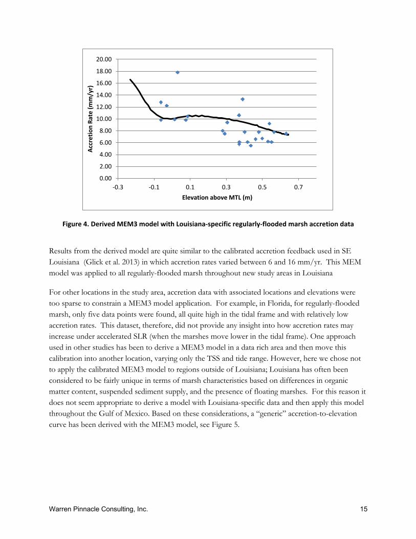
The vast majority of accretion data with relevant elevations are located in Louisiana and a MEM3 model was derived for this location. A graph of this relationship and the data used to derive it is shown in Figure 3. To achieve this Louisiana-specific MEM3 model, the biomass range was extended to well above Mean Higher High water which is likely reasonable in this microtidal region. The organic matter contribution to accretion also was boosted to support relatively high accretion rates that data show occur at 0.5 meters above MTL and higher. This model suggests that accretion rates will vary between 7.0 and 16 mm/yr. depending on location in the tidal frame.
Warren Pinnacle Consulting, Inc. 15
Figure 4. Derived MEM3 model with Louisiana-specific regularly-flooded marsh accretion data
Results from the derived model are quite similar to the calibrated accretion feedback used in SE Louisiana (Glick et al. 2013) in which accretion rates varied between 6 and 16 mm/yr. This MEM model was applied to all regularly-flooded marsh throughout new study areas in Louisiana
For other locations in the study area, accretion data with associated locations and elevations were too sparse to constrain a MEM3 model application. For example, in Florida, for regularly-flooded marsh, only five data points were found, all quite high in the tidal frame and with relatively low accretion rates. This dataset, therefore, did not provide any insight into how accretion rates may increase under accelerated SLR (when the marshes move lower in the tidal frame). One approach used in other studies has been to derive a MEM3 model in a data rich area and then move this calibration into another location, varying only the TSS and tide range. However, here we chose not to apply the calibrated MEM3 model to regions outside of Louisiana; Louisiana has often been considered to be fairly unique in terms of marsh characteristics based on differences in organic matter content, suspended sediment supply, and the presence of floating marshes. For this reason it does not seem appropriate to derive a model with Louisiana-specific data and then apply this model throughout the Gulf of Mexico. Based on these considerations, a “generic” accretion-to-elevation curve has been derived with the MEM3 model, see Figure 5.
0.00
2.00
4.00
6.00
8.00
10.00
12.00
14.00
16.00
18.00
20.00
-0.3 -0.1 0.1 0.3 0.5 0.7
Accr
etio
n Ra
te (m
m/y
r)
Elevation above MTL (m)

Warren Pinnacle Consulting, Inc. 16
Figure 5. Generic MEM3 curve
Minimum and maximum accretion rates were then modified on the basis of local conditions to account for measured accretion data, spatial variability in TSS data, and professional judgments. The following accretion regions have been defined based on TSS:
• Southern Florida (South of Big Bend study area) - Mean TSS of 8 mg/L
• Northern Florida (Big Bend of Florida north) - Mean TSS of 10 mg/L
• Alabama, excluding Mobile Bay - Mean TSS of 11 mg/L
• Mobile Bay - Higher TSS (16 mg/L) and site-specific accretion data
• Mississippi - Mean TSS of 34 mg/L
• Louisiana - Calibrated accretion feedback in existing study areas and MEM model in non-
modeled locations (Chenier Plain), TSS set to 26 mg/L
• Northern Texas (to Freeport) - Calibrated accretion feedbacks in existing study areas and MEM3
for Jefferson County, mean TSS of 30 mg/L
• Freeport, Texas South to Mexican border - mean TSS of 36 mg/L
TSS data presented above were derived first by querying individual data points from EPA STORET and then assigning these points to each defined study area. In order to remove data artifacts and the effects of unique events that may not reflect the average TSS conditions affecting marshes, the top

Warren Pinnacle Consulting, Inc. 17
and bottom 2.5% of TSS data were discarded. Study areas were combined and averaged to obtain a spatially weighted average TSS for each region. These data have been qualitatively considered, as part of the weight of evidence approach in determining reasonable accretion-feedback curves for each region. Accretion models for each region are described below:
Southern Florida. Analysis of the accretion database created for this project indicates a minimum accretion rate of 0.8 mm/year and maximum measured accretion rates of 4.9 mm/yr. This is consistent with regularly-flooded marsh accretion rates applied in Florida given previous SLAMM applications. It is also consistent with observations of TSS that are lowest among the accretion regions defined above. As increased SLR has not started to drown regularly-flooded marshes in this portion of the study area yet (at least in areas that we have accretion data), the upper bound accretion rate is uncertain. However, based on TSS availability it is safe to presume that it should be less than the 16 mm/yr. measured in Louisiana. Constraining the maximum accretion rate to the maximum accretion rate measured in the region seems like a reasonable conjecture. In the future, the uncertainty in the model based on this conjecture can be measured with a SLAMM uncertainty analysis. In addition, as will be the case for most study areas, additional observed data regarding marsh accretion rates at elevation (marsh organ studies), marsh biomass densities, and inorganic sediment settling rates can improve the accuracy of future SLR simulations. To summarize, for S. Florida salt marshes were modeled with accretion feedbacks and minimum accretion rates of 0.8 mm/yr. and maximums of 4.9 mm/yr.
Northern Florida. TSS concentrations increase relative to S. Florida as do maximum accretion rates observed. For this reason a similar relationship between accretion rates and elevations is assumed, but with the maximum accretion rate being set to 7.6 mm/yr. (maximum observed in the study area, measured by Leonard et al 1995) and minimum accretion rate set to 0.8 mm/yr. (Cahoon et al. 1995, Hendrickson 1997, net elevation change). Florida is the only portion of the study area with a useful database of elevation change data, measured by SET tables maintained by the Florida Geologic Survey. These data were provided to WPC in 2011 by Joe Donoghue in support of the Saint Andrew’s Choctawhatchee modeling effort funded by TNC. These rates cover the same range as previously applied to other SLAMM applications in this region (0.8 mm/yr. in Apalachicola to 7.2 mm/yr. in Southern Big Bend).
Alabama excluding Mobile Bay. A maximum accretion rate of 6.8 mm/yr. was applied based on somewhat lower TSS than Northern Florida and the accretion data of Callaway (1997). This value was applied without feedbacks to previous SLAMM applications in Mississippi.
Mobile Bay, Alabama. The minimum accretion rate is set to 0.9 mm/yr. and the maximum accretion rate to 11 mm/yr. (Smith et al. 2013) based on the higher TSS observed in this region and observed accretion data cited above. The Smith reference also informed the previous application of SLAMM to Mobile Bay.
Warren Pinnacle Consulting, Inc. 18
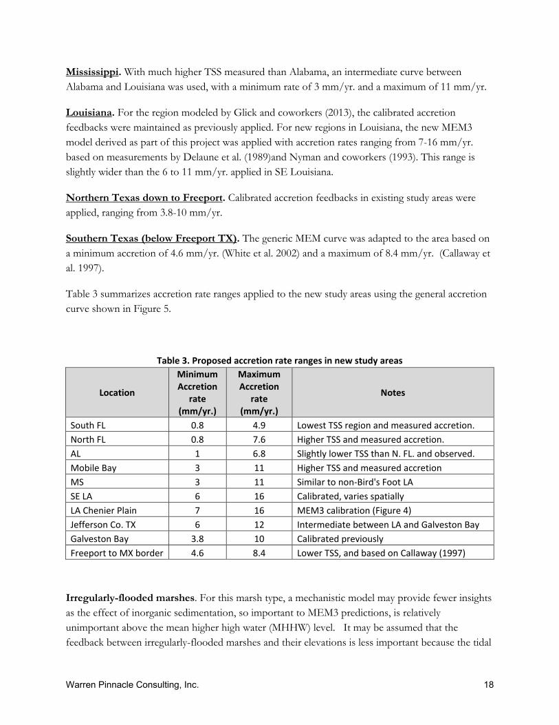
Mississippi. With much higher TSS measured than Alabama, an intermediate curve between Alabama and Louisiana was used, with a minimum rate of 3 mm/yr. and a maximum of 11 mm/yr.
Louisiana. For the region modeled by Glick and coworkers (2013), the calibrated accretion feedbacks were maintained as previously applied. For new regions in Louisiana, the new MEM3 model derived as part of this project was applied with accretion rates ranging from 7-16 mm/yr. based on measurements by Delaune et al. (1989)and Nyman and coworkers (1993). This range is slightly wider than the 6 to 11 mm/yr. applied in SE Louisiana.
Northern Texas down to Freeport. Calibrated accretion feedbacks in existing study areas were applied, ranging from 3.8-10 mm/yr.
Southern Texas (below Freeport TX). The generic MEM curve was adapted to the area based on a minimum accretion of 4.6 mm/yr. (White et al. 2002) and a maximum of 8.4 mm/yr. (Callaway et al. 1997).
Table 3 summarizes accretion rate ranges applied to the new study areas using the general accretion curve shown in Figure 5.
Table 3. Proposed accretion rate ranges in new study areas
Location
Minimum Accretion
rate (mm/yr.)
Maximum Accretion
rate (mm/yr.)
Notes
South FL 0.8 4.9 Lowest TSS region and measured accretion. North FL 0.8 7.6 Higher TSS and measured accretion. AL 1 6.8 Slightly lower TSS than N. FL. and observed. Mobile Bay 3 11 Higher TSS and measured accretion MS 3 11 Similar to non-Bird's Foot LA SE LA 6 16 Calibrated, varies spatially LA Chenier Plain 7 16 MEM3 calibration (Figure 4) Jefferson Co. TX 6 12 Intermediate between LA and Galveston Bay Galveston Bay 3.8 10 Calibrated previously Freeport to MX border 4.6 8.4 Lower TSS, and based on Callaway (1997)
Irregularly-flooded marshes. For this marsh type, a mechanistic model may provide fewer insights as the effect of inorganic sedimentation, so important to MEM3 predictions, is relatively unimportant above the mean higher high water (MHHW) level. It may be assumed that the feedback between irregularly-flooded marshes and their elevations is less important because the tidal

Warren Pinnacle Consulting, Inc. 19
flooding which drives this process is much less regular. For this reason, and also based on data limitations, the accretion of irregularly-flooded marshes was not modeled using MEM3. A constant accretion rate was instead applied as done in previous model applications.
Mangrove. Elevation change data collected in Florida suggests an accretion rate of 2 mm/yr. (Cahoon and Lynch 1997; Donoghue 2011; McKee 2011) This is lower than the rates of 7 mm/yr. and 3.3 mm/yr. previously applied in the gulf; however, it is more appropriate since SLAMM tracks elevation change.
Regarding mangrove distribution, mangroves in Florida up to Tampa Bay were modeled based on previous SLAMM applications and the findings of Osland and coworkers (2013). When the SLAMM model finds adequate mangrove coverage in a site, it designates that site as “tropical” and all wetland to wetland or dry land to wetland conversions become mangroves. Therefore, mangroves tend to dominate these sites under conditions of SLR. In Florida, north of the Tampa Bay study area, previous SLAMM applications were not designated as “tropical.” It is certainly possible that mangroves will continue to migrate further north in the next 85 years and this is not represented by these simulations. The northern boundary of mangrove habitat tends to be driven by the “hard freeze” line and air temperature is not a driving variable within SLAMM applications. Furthermore, the boundary of mangrove habitat is patchy and uncertain and can be variable from year to year. No mangrove expansions in Texas, Louisiana, MS, or AL are predicted by this modeling exercise, either, consistent with previous applications of SLAMM in those states.
Tidal and Inland Fresh Marsh. A gap analysis was used to apply accretion rates to unmodeled areas: The values applied to adjacent areas were extrapolated based on site characteristics and professional judgment.
Swamp and Tidal Swamp. For all previous Gulf SLAMM analyses, excluding the Atchafalaya Basin, swamp and tidal swamp accretion rates were set to 0.3 and 1.1 mm/yr., respectively. Due to a lack of data to determine more appropriate site-specific rates, and to maintain consistency with previous model applications, these rates were applied throughout the entire Gulf.
Model Calibration
Once a SLAMM project is set up with all raster layers and initial parameterization, SLAMM is run at “time zero.” At this time step only the tides are applied to the study area while no SLR, accretion or erosion is considered. These “time zero projections” allow model users to assess the consistency between elevation data, the current land coverage, modeled tidal ranges and hydraulic connectivity. Generally, due to local factors, DEM and NWI uncertainty, and simplifications within the SLAMM conceptual model, some cells will initially be below their lowest allowable elevation category and are immediately converted by the model to a different land cover category. For example, an area categorized in the wetland layer as fresh-water swamp but which is subject to regular saline tides,

Warren Pinnacle Consulting, Inc. 20
according to its elevation and tidal information, is converted by SLAMM to a tidal marsh at time zero. Or initially areas identified as marsh are not regularly inundated because either the tidal ranges are not correct or there are impediments in the elevation layer that require to be removed to further hydro-enforce the DEMs.
Where significant land cover changes occur, additional investigation may be required to confirm that the current land cover of a particular area is correctly represented. If not, it is sometimes necessary to better calibrate data layers and model inputs to the actual observed conditions. The general rule of thumb is that if 95% of a major land cover category (one covering ≥ 5% of the study area) is not converted at time zero, then the model set-up is considered acceptable. However, land coverage conversion maps at time zero are always reviewed to identify initial problems, if any, and necessary adjustments to correct them.
In some cases the initial land cover re-categorization by SLAMM better describes the current coverage of a given area. For example, the high horizontal resolution of the elevation data can allow for a more refined wetland map than the original NWI-generated shapefiles used in this project. Therefore, if time zero maps include changes that are supported by satellite imagery or local knowledge of wetland types, then these types of land cover conversion are then accepted without further investigation.
Elevation Pre-processor
SLAMM can model areas with lower-quality elevation data by applying the “elevation pre-processor” module. When required, SLAMM estimates coastal-wetland elevation ranges as a function of tide ranges and known relationships between wetland types and tide ranges. However, this method is subject to error and uncertainty.
Fortunately the vast majority of the GCPLCC study area is covered with high-resolution LiDAR data. In terms of new study areas, the exceptions were some inland areas in South Florida (small inland portions of study areas 1, 2, & 3), Area 16 (the Dry Tortugas, Florida), and far inland north of Mobile Bay (portions of study area 12). With regards to existing model results, the sole exception was the Key West National Wildlife Refuge study area.
The elevation pre-processor works by processing wetland elevations unidirectionally away from open water. The front edge of each wetland type is assigned a minimum elevation, specific to the wetland category that it falls into. The back edge of each wetland type is given the maximum elevation for that category. The slope and elevations of intermediate cells are interpolated between these two points. The model assumes that wetland elevations are uniformly distributed over their feasible vertical elevation ranges or “tidal frames”—an assumption that may not reflect reality. If wetlands elevations are actually clustered high in the tidal frame they would be less vulnerable to SLR and if elevations are towards the bottom, they would be more vulnerable. LiDAR data for any

Warren Pinnacle Consulting, Inc. 21
site assists in reducing model uncertainty by characterizing where these marshes exist in their expected range.
As a test of how the elevation pre-processor may change model predictions, we performed an analysis of low-quality elevation data effects in this project. We chose two model domains with high-quality data, converted these data to “contour equivalent” elevations, and then ran the model with the elevation pre-processor. These results were compared with model results based on LiDAR. The results of this analysis may be found in the “Results and Discussion” section.
Freshwater Flow Polygons
Within SLAMM, a polygon may be defined as having freshwater-flow influence without explicitly modeling salinity—this modifies the habitat-switching flow chart. This is often done along large rivers and their tributaries. In this modified flow chart Dry Land or Swamp converts to Tidal Swamp, Tidal Swamp converts to Tidal Fresh Marsh, and Tidal Fresh Marsh then converts to Irregularly-Flooded Marsh. In comparison, when no freshwater influence is defined, Swamp converts directly to Irregularly-Flooded Marsh and dry lands convert to transitional salt marsh.
Flooded Swamp
Several areas along the Gulf coast are populated by cypress swamps. For the NWF-funded application of SLAMM to Southeast LA, SLAMM was adjusted to predict that cypress swamps convert to permanently “flooded swamp” when their elevations falls to a level below which non-flooded land will rarely be exposed. This designation was added to denote swamps that may still include live plants but which are not expected to remain viable for long as they are not able to germinate.
Cypress swamps often occur at elevations of 2m above mean sea level or less (Allen et al. 1996) and may be regularly inundated with standing water. Bald cypress has been found to be highly tolerant of flooding, though germination is not possible under permanent flooding conditions (Allen et al. 1996). In a study of wetland tree growth-response to flooding, Keeland and coworkers found permanent shallow flooding of approximately 25 cm occurred in the area of the Barataria basin swamp under examination (1997). In addition, site-specific data suggest that this elevation is the lowest elevation inhabited by this wetland type.
The addition of “flooded swamp” is a bit of a departure from SLAMM conventions. Generally, SLAMM estimates what will happen if a given habitat comes to equilibrium with the water levels predicted a given time step. However, given the length of time that cypress trees can remain alive within flooded swamps, assuming immediate conversion to open water may provide misleading model results.

Warren Pinnacle Consulting, Inc. 22
Considerations for individual study areas
This section provides a brief description of the distinguishing characteristics, if any, of each of the new study sites.
Figure 6. New Study Areas in Florida
9
8
7
5
6
4
3
2
1
21
16

Warren Pinnacle Consulting, Inc. 23
Figure 7. New Study Areas in Northern Florida, Alabama, Mississippi, and Louisiana
Figure 8. New Study Areas in Texas
1417
12
1011
13
20
18
19
Warren Pinnacle Consulting, Inc. 24
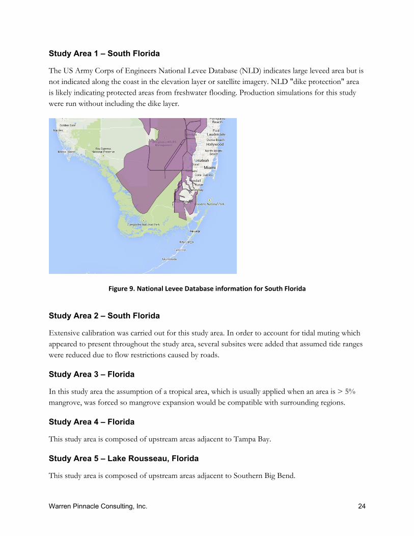
Study Area 1 – South Florida
The US Army Corps of Engineers National Levee Database (NLD) indicates large leveed area but is not indicated along the coast in the elevation layer or satellite imagery. NLD "dike protection" area is likely indicating protected areas from freshwater flooding. Production simulations for this study were run without including the dike layer.
Figure 9. National Levee Database information for South Florida
Study Area 2 – South Florida
Extensive calibration was carried out for this study area. In order to account for tidal muting which appeared to present throughout the study area, several subsites were added that assumed tide ranges were reduced due to flow restrictions caused by roads.
Study Area 3 – Florida
In this study area the assumption of a tropical area, which is usually applied when an area is > 5% mangrove, was forced so mangrove expansion would be compatible with surrounding regions.
Study Area 4 – Florida
This study area is composed of upstream areas adjacent to Tampa Bay.
Study Area 5 – Lake Rousseau, Florida
This study area is composed of upstream areas adjacent to Southern Big Bend.

Warren Pinnacle Consulting, Inc. 25
Study Area 6 – Florida
This is an inland area adjacent to Southern Big Bend and Lower Suwanee.
Study Area 7 – Florida
This study area upstream of the Lower Suwannee River
Study Area 8 – Florida
Muted tide ranges were applied to the NW corner of the study area.
Study Area 9 – St. Joe Bay and Carabelle, Florida
In this study area some wetland areas were edited. In south St. Joseph’s Bay, inland fresh marshes that, according to aerial photography, should have been beach were converted to estuarine beach.
Study Area 10 – Florida
This study area is located upstream of the Pensacola study area. SLAMM input parameters were taken from an adjacent subsite area in the older Pensacola study.
Study Areas 11 and 13 - Florida
This study area is composed of upstream areas adjacent to Perdido Bay. SLAMM input parameters were taken from an adjacent subsite area in the older Perdido Bay study.
Study Area 12 – Alabama
This study is located upstream of the Mobile Bay study area. A freshwater flow polygon was added to the entire study area. SLAMM input parameters were taken from an adjacent subsite area in the older Mobile Bay study.
Study Area 14 – Mississippi and Louisiana
SLAMM input parameters were taken from an adjacent subsite areas in older studies. Subsidence was added by adjusting historic SLR rate and applying the average rate for the area based on the data of Shinkle and Dokka (2004). Input data were divided based on the rates for each state, LA in the west and MS in the east. In addition, a freshwater flow polygon was added to northern Bayou Sauvage to match the freshwater extent applied in the Bayou Sauvage study area.
(Study Area 15 does not exist in this study-- it was possible to include this area in an adjacent study area.)
Warren Pinnacle Consulting, Inc. 26
Study Area 16 – Dry Tortugas, Florida
Due to low-quality elevation data the elevation pre-processor was used for the entirety extent of this study area.
Study Area 17 – Louisiana Chenier Plain
In Louisiana, since the input wetland data from Couvillion (2011) does not include tidal fresh marsh, it was necessary to add this wetland type where tidal fresh was classified simply as inland fresh. This approach was also used in the previous applications of SLAMM to Southeast Louisiana (Glick et al. 2013). Subsidence was added by adjusting historic SLR rate and applying the average rate for the area based on the data of Shinkle and Dokka (2004)
One of the difficulties in modeling this area was the lack of knowledge regarding levees, many of which are private and are not always apparent in the elevation layer due to averaging within a cell. Despite our best efforts to procure a detailed levee database, the simulation run does not account for all the existing flood control structures within the study area. In setting up this site we were able to add levees based on a conversation with Schuyler Dartez at White Lake Wetlands Conservation Area (WCA), the entirety of the WCA is impounded/leveed and all water levels are controlled by rainfall, not tides. Therefore we designated the entire area as diked.
To improve the initial model calibration several steps were taken, including adjusting the tide range based on CRMS tide data at station CRMS0567 and adding two freshwater flow polygons (one around the Atchafalaya River and another around the Sabine River). In addition, it is important to note horizontal linear artifacts in elevation data north of Maurepas show up in the time-zero (calibration step) and some future predictions, increasing uncertainty in the model predictions in these regions.
Study Area 18 – Galveston Bay, Texas
Subsite parameters for this site were added from adjacent Galveston subsites.
Study Area 19 – Matagorda and San Antonio Bays, Texas
Though the majority of the subsites in this study area were added to reflect differences in tide ranges, some input subsites were added based on erosion data. In particular, subsites were added around the Matagorda Ship Channel and Pass Cavallo to reflect the high rates of erosion observed in those areas.
Study Area 20 – Baffin Bay, South Texas
Radosavljevic and coworkers have suggested a historic SLR in the Mustang Island area ranged between 3.4-5.2 mm yr. for the past fifty to sixty years (2012). In comparison, we applied a Historic

Warren Pinnacle Consulting, Inc. 27
Trend of 3.17mm/yr. to the area, which was the average of the values applied in the existing Lower Rio Grande and Corpus Christi project areas.
Study Area 21 – Florida
This area closes a small gap between Tampa Bay and Southern Big Bend study areas.
Focal Species Approach
As part of this project, an analysis was performed to assess the impact of SLR on focal species through the generation of patch metrics for each species’ habitat. The GCPLCC technical team provided the focal species choices which were all avian species: seaside sparrow, mottled duck, and black skimmer. One or more wildlife habitat relationship models (WHRM) were developed for each species by identifying one or more SLAMM cover categories (patch classes) upon which the species is dependent. In some cases, queries were developed that required spatial (patch size) constraints.
Table 4. Models specified by GCPLCC staff and their partners Species Name Species
Code SLAMM Category Code – Name Spatial Query / Note
Seaside sparrow SESA 8 – Regularly Flooded Marsh 20 – Irregularly Flooded Marsh
Number and proportion of polygons > 10,000 acres
Mottled duck MODU 6 – Tidal Fresh Marsh 7 – Transitional Marsh / Scrub Shrub 20 – Irregularly Flooded Marsh
Mottled duck MODU 17 – Estuarine Open Water Number and proportion of polygons > 640 acres (=1 mile2)
Black skimmer BLSK 10 – Estuarine Beach 12 – Ocean Beach
Note that polygons were generated from an aggregation of both SLAMM categories.
Black skimmer BLSK 10 – Estuarine Beach Black skimmer BLSK 12 – Ocean Beach
A number of summary metrics were produced for each WHRM at each time step in each scenario. This resulted in 150 unique combinations (6 WHRMs × 5 scenarios × 5 time steps). Summary metrics include:
• The number of patches (when combined with total raw area, can calculate mean patch size); • The mean patch area; • The P/A ratio (best measure of shape complexity that can be generated with tools identified
at present).

Warren Pinnacle Consulting, Inc. 28
In addition, the following data product was produced for each WHRM at each time step in each scenario, so patch distributions can be developed as needed in the future:
• Patch Data Table (.dbf format; 150 unique files, zipped together for a project deliverable)
The specific processing steps used to generate the summary patch metric statistics for each WHRM at each time step for each scenario are as follows:
1. Create a new raster output in Project projection (Albers_USGS, NAD83) with15m resolution, snapped to project grid, for all output from existing studies.
2. Mosaic all new study area output and that from existing studies into single rasters (5 scenarios X 5 time steps = 25 unique rasters). For existing studies, all base years merged to same “base” condition.
3. Reclassify mosaicked rasters to these 6 species-specific habitat rasters (6 X 25 scenario-time steps = 150 unique rasters), utilizing the WHRMs presented above.
4. Convert 150 species-specific habitat rasters to polygons (no polygon simplification / generalization)
5. Add area (Area_m2), perimeter (Perimeterm), and P/A ratio (P2A_ratio) attributes
6. Calculate geometry for area and perimeter attributes, and then calculate P/A ratio attribute.
7. Generate summary (patch metric) statistics and compile into single tables for each WHRM.
Finally, the WHRM tables (spreadsheets) were compiled into an Excel workbook as a project deliverable.
Warren Pinnacle Consulting, Inc. 29
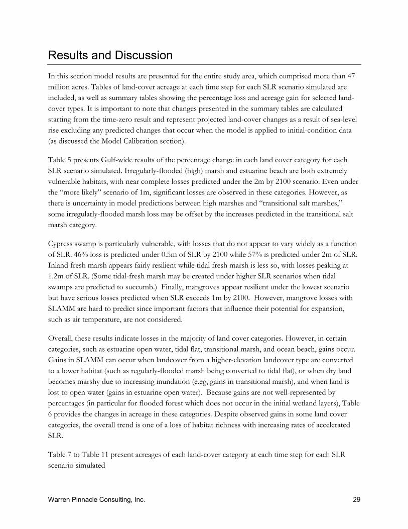
Results and Discussion In this section model results are presented for the entire study area, which comprised more than 47 million acres. Tables of land-cover acreage at each time step for each SLR scenario simulated are included, as well as summary tables showing the percentage loss and acreage gain for selected land-cover types. It is important to note that changes presented in the summary tables are calculated starting from the time-zero result and represent projected land-cover changes as a result of sea-level rise excluding any predicted changes that occur when the model is applied to initial-condition data (as discussed the Model Calibration section).
Table 5 presents Gulf-wide results of the percentage change in each land cover category for each SLR scenario simulated. Irregularly-flooded (high) marsh and estuarine beach are both extremely vulnerable habitats, with near complete losses predicted under the 2m by 2100 scenario. Even under the “more likely” scenario of 1m, significant losses are observed in these categories. However, as there is uncertainty in model predictions between high marshes and “transitional salt marshes,” some irregularly-flooded marsh loss may be offset by the increases predicted in the transitional salt marsh category.
Cypress swamp is particularly vulnerable, with losses that do not appear to vary widely as a function of SLR. 46% loss is predicted under 0.5m of SLR by 2100 while 57% is predicted under 2m of SLR. Inland fresh marsh appears fairly resilient while tidal fresh marsh is less so, with losses peaking at 1.2m of SLR. (Some tidal-fresh marsh may be created under higher SLR scenarios when tidal swamps are predicted to succumb.) Finally, mangroves appear resilient under the lowest scenario but have serious losses predicted when SLR exceeds 1m by 2100. However, mangrove losses with SLAMM are hard to predict since important factors that influence their potential for expansion, such as air temperature, are not considered.
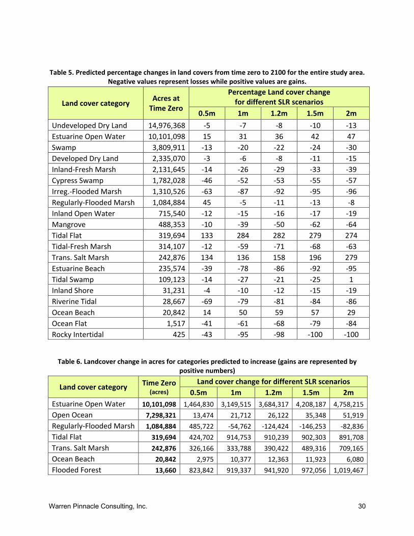
Overall, these results indicate losses in the majority of land cover categories. However, in certain categories, such as estuarine open water, tidal flat, transitional marsh, and ocean beach, gains occur. Gains in SLAMM can occur when landcover from a higher-elevation landcover type are converted to a lower habitat (such as regularly-flooded marsh being converted to tidal flat), or when dry land becomes marshy due to increasing inundation (e.eg, gains in transitional marsh), and when land is lost to open water (gains in estuarine open water). Because gains are not well-represented by percentages (in particular for flooded forest which does not occur in the initial wetland layers), Table 6 provides the changes in acreage in these categories. Despite observed gains in some land cover categories, the overall trend is one of a loss of habitat richness with increasing rates of accelerated SLR.
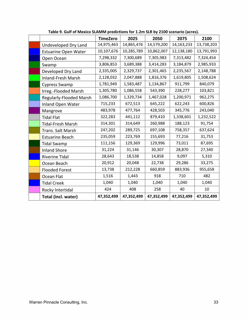
Table 7 to Table 11 present acreages of each land-cover category at each time step for each SLR scenario simulated
Warren Pinnacle Consulting, Inc. 30
Table 5. Predicted percentage changes in land covers from time zero to 2100 for the entire study area. Negative values represent losses while positive values are gains.
Land cover category Acres at Time Zero
Percentage Land cover change for different SLR scenarios
0.5m 1m 1.2m 1.5m 2m Undeveloped Dry Land 14,976,368 -5 -7 -8 -10 -13 Estuarine Open Water 10,101,098 15 31 36 42 47 Swamp 3,809,911 -13 -20 -22 -24 -30 Developed Dry Land 2,335,070 -3 -6 -8 -11 -15 Inland-Fresh Marsh 2,131,645 -14 -26 -29 -33 -39 Cypress Swamp 1,782,028 -46 -52 -53 -55 -57 Irreg.-Flooded Marsh 1,310,526 -63 -87 -92 -95 -96 Regularly-Flooded Marsh 1,084,884 45 -5 -11 -13 -8 Inland Open Water 715,540 -12 -15 -16 -17 -19 Mangrove 488,353 -10 -39 -50 -62 -64 Tidal Flat 319,694 133 284 282 279 274 Tidal-Fresh Marsh 314,107 -12 -59 -71 -68 -63 Trans. Salt Marsh 242,876 134 136 158 196 279 Estuarine Beach 235,574 -39 -78 -86 -92 -95 Tidal Swamp 109,123 -14 -27 -21 -25 1 Inland Shore 31,231 -4 -10 -12 -15 -19 Riverine Tidal 28,667 -69 -79 -81 -84 -86 Ocean Beach 20,842 14 50 59 57 29 Ocean Flat 1,517 -41 -61 -68 -79 -84 Rocky Intertidal 425 -43 -95 -98 -100 -100
Table 6. Landcover change in acres for categories predicted to increase (gains are represented by positive numbers)
Land cover category Time Zero (acres)
Land cover change for different SLR scenarios 0.5m 1m 1.2m 1.5m 2m
Estuarine Open Water 10,101,098 1,464,830 3,149,515 3,684,317 4,208,187 4,758,215 Open Ocean 7,298,321 13,474 21,712 26,122 35,348 51,919 Regularly-Flooded Marsh 1,084,884 485,722 -54,762 -124,424 -146,253 -82,836 Tidal Flat 319,694 424,702 914,753 910,239 902,303 891,708 Trans. Salt Marsh 242,876 326,166 333,788 390,422 489,316 709,165 Ocean Beach 20,842 2,975 10,377 12,363 11,923 6,080 Flooded Forest 13,660 823,842 919,337 941,920 972,056 1,019,467

Warren Pinnacle Consulting, Inc. 31
Table 7. Gulf of Mexico SLAMM predictions for 0.5m SLR by 2100 scenario (acres). Time Zero 2025 2050 2075 2100
Undeveloped Dry Land
Undeveloped Dry Land 14,976,368 14,900,438 14,733,636 14,530,181 14,267,948 Estuarine Open Water
Estuarine Open Water 10,101,098 10,226,614 10,456,046 10,889,717 11,565,929
Open Ocean Open Ocean 7,298,321 7,300,223 7,303,010 7,306,784 7,311,795
Swamp Swamp 3,809,911 3,751,446 3,601,518 3,457,104 3,301,153
Developed Dry Land
Developed Dry Land 2,335,070 2,332,315 2,320,548 2,298,659 2,262,719 Inland-Fresh Marsh
Inland-Fresh Marsh 2,131,645 2,099,638 2,019,436 1,921,310 1,828,235 Cypress Swamp
Cypress Swamp 1,782,028 1,654,297 1,369,506 1,118,148 958,226 Irreg.-Flooded Marsh
Irreg.-Flooded Marsh 1,310,526 1,209,073 984,639 675,011 487,830 Regularly-Flooded Marsh
Regularly-Flooded Marsh 1,084,884 1,234,457 1,416,782 1,646,427 1,570,606 Inland Open Water
Inland Open Water 715,540 679,347 656,794 640,068 627,931
Mangrove Mangrove 488,353 487,462 479,416 464,691 439,532
Tidal Flat Tidal Flat 319,694 389,412 471,561 613,979 744,396
Tidal-Fresh Marsh
Tidal-Fresh Marsh 314,107 319,158 295,376 271,001 276,544 Trans. Salt Marsh
Trans. Salt Marsh 242,876 213,214 400,589 463,709 569,042 Estuarine Beach
Estuarine Beach 235,574 230,594 221,291 178,287 143,852
Tidal Swamp Tidal Swamp 109,123 110,720 126,102 132,891 94,352
Inland Shore Inland Shore 31,231 31,180 31,104 30,876 30,118
Riverine Tidal
Riverine Tidal 28,667 18,875 15,696 11,439 8,802
Ocean Beach Ocean Beach 20,842 19,656 20,387 21,896 23,818
Flooded Forest
Flooded Forest 13,660 141,409 426,208 677,577 837,502
Ocean Flat Ocean Flat 1,517 1,513 1,417 1,348 890
Tidal Creek Tidal Creek 1,040 1,040 1,040 1,040 1,040
Rocky Intertidal
Rocky Intertidal 425 419 396 355 241
Total (incl. water) 47,352,499 47,352,499 47,352,499 47,352,499 47,352,499

Warren Pinnacle Consulting, Inc. 32
Table 8. Gulf of Mexico SLAMM predictions for 1m SLR by 2100 scenario (acres). TimeZero 2025 2050 2075 2100
Undeveloped Dry Land
Undeveloped Dry Land 14,975,734 14,875,495 14,623,215 14,263,507 13,899,386 Estuarine Open Water
Estuarine Open Water 10,105,826 10,267,089 10,729,052 11,766,755 13,255,341
Open Ocean Open Ocean 7,298,329 7,300,494 7,304,944 7,311,675 7,320,041
Swamp Swamp 3,807,645 3,709,778 3,456,383 3,245,112 3,062,487
Developed Dry Land
Developed Dry Land 2,335,027 2,330,514 2,307,353 2,255,830 2,186,791 Inland-Fresh Marsh
Inland-Fresh Marsh 2,129,137 2,063,207 1,879,999 1,688,803 1,581,418 Cypress Swamp
Cypress Swamp 1,781,976 1,604,312 1,194,973 941,480 862,687 Irreg.-Flooded Marsh
Irreg.-Flooded Marsh 1,307,105 1,124,080 653,331 311,561 168,863 Regularly-Flooded Marsh
Regularly-Flooded Marsh 1,085,862 1,300,535 1,508,647 1,317,683 1,031,100 Inland Open Water
Inland Open Water 715,370 673,964 648,168 626,062 607,209
Mangrove Mangrove 485,132 480,423 449,446 385,094 296,802
Tidal Flat Tidal Flat 321,884 425,115 731,416 1,193,127 1,236,637
Tidal-Fresh Marsh
Tidal-Fresh Marsh 314,245 316,359 272,095 234,640 130,408 Trans. Salt Marsh
Trans. Salt Marsh 245,878 264,986 613,583 709,968 579,667 Estuarine Beach
Estuarine Beach 235,191 227,277 172,461 102,929 52,720
Tidal Swamp Tidal Swamp 110,698 124,782 136,875 75,514 80,969
Inland Shore Inland Shore 31,225 31,159 30,354 29,868 28,012
Riverine Tidal Riverine Tidal 28,649 18,631 15,082 9,588 5,987
Ocean Beach Ocean Beach 20,894 19,947 21,928 27,028 31,270
Flooded Forest
Flooded Forest 13,712 191,401 600,748 854,254 933,049
Ocean Flat Ocean Flat 1,516 1,499 1,128 767 595
Tidal Creek Tidal Creek 1,040 1,040 1,040 1,040 1,040
Rocky Intertidal
Rocky Intertidal 425 412 278 215 20 Total (incl. water) 47,352,499 47,352,499 47,352,499 47,352,499 47,352,499
Warren Pinnacle Consulting, Inc. 33
Table 9. Gulf of Mexico SLAMM predictions for 1.2m SLR by 2100 scenario (acres). TimeZero 2025 2050 2075 2100
Undeveloped Dry Land
Undeveloped Dry Land 14,975,463 14,865,476 14,579,200 14,163,233 13,738,203 Estuarine Open Water
Estuarine Open Water 10,107,676 10,285,789 10,862,007 12,138,180 13,791,993
Open Ocean Open Ocean 7,298,332 7,300,689 7,305,983 7,313,482 7,324,454
Swamp Swamp 3,806,853 3,689,388 3,414,283 3,184,879 2,985,933
Developed Dry Land
Developed Dry Land 2,335,005 2,329,737 2,301,465 2,235,567 2,148,788 Inland-Fresh Marsh
Inland-Fresh Marsh 2,128,032 2,047,888 1,816,376 1,619,805 1,508,624 Cypress Swamp
Cypress Swamp 1,781,949 1,583,487 1,134,867 911,799 840,079 Irreg.-Flooded Marsh
Irreg.-Flooded Marsh 1,305,780 1,086,558 543,390 228,277 103,821 Regularly-Flooded Marsh
Regularly-Flooded Marsh 1,086,700 1,329,734 1,467,028 1,200,971 962,275 Inland Open Water
Inland Open Water 715,233 672,513 645,222 622,243 600,826
Mangrove Mangrove 483,978 477,764 428,503 345,776 243,040
Tidal Flat Tidal Flat 322,283 441,112 879,410 1,338,601 1,232,522
Tidal-Fresh Marsh
Tidal-Fresh Marsh 314,301 314,649 260,988 188,123 91,754 Trans. Salt Marsh
Trans. Salt Marsh 247,202 289,725 697,108 758,357 637,624 Estuarine Beach
Estuarine Beach 235,059 223,769 155,693 77,216 31,753
Tidal Swamp Tidal Swamp 111,156 129,369 129,996 73,011 87,695
Inland Shore Inland Shore 31,224 31,146 30,307 28,870 27,340
Riverine Tidal Riverine Tidal 28,643 18,538 14,858 9,097 5,310
Ocean Beach Ocean Beach 20,912 20,048 22,738 29,286 33,275
Flooded Forest
Flooded Forest 13,738 212,228 660,859 883,936 955,658
Ocean Flat Ocean Flat 1,516 1,443 918 710 482
Tidal Creek Tidal Creek 1,040 1,040 1,040 1,040 1,040
Rocky Intertidal
Rocky Intertidal 424 408 258 40 10 Total (incl. water) 47,352,499 47,352,499 47,352,499 47,352,499 47,352,499

Warren Pinnacle Consulting, Inc. 34
Table 10. Gulf of Mexico SLAMM predictions for 1.5m SLR by 2100 scenario (acres). TimeZero 2025 2050 2075 2100
Undeveloped Dry Land
Undeveloped Dry Land 14,974,980 14,848,880 14,509,006 14,006,439 13,506,422 Estuarine Open Water
Estuarine Open Water 10,110,515 10,345,832 11,082,044 12,658,142 14,318,701
Open Ocean Open Ocean 7,298,312 7,300,940 7,307,053 7,316,737 7,333,660
Swamp Swamp 3,805,638 3,660,612 3,357,186 3,088,564 2,877,650
Developed Dry Land
Developed Dry Land 2,334,979 2,328,465 2,291,097 2,201,268 2,085,236 Inland-Fresh Marsh
Inland-Fresh Marsh 2,126,252 2,021,636 1,734,566 1,536,682 1,424,412 Cypress Swamp
Cypress Swamp 1,781,892 1,549,566 1,058,716 880,374 809,894 Irreg.-Flooded Marsh
Irreg.-Flooded Marsh 1,303,828 1,025,028 410,817 135,143 63,882 Regularly-Flooded Marsh
Regularly-Flooded Marsh 1,087,854 1,371,972 1,359,096 1,156,545 941,601 Inland Open Water
Inland Open Water 715,138 669,811 641,607 614,358 592,562
Mangrove Mangrove 482,126 472,600 397,001 275,018 181,170
Tidal Flat Tidal Flat 322,919 457,108 1,110,626 1,379,767 1,225,221
Tidal-Fresh Marsh
Tidal-Fresh Marsh 314,380 311,144 236,888 127,720 99,468 Trans. Salt Marsh
Trans. Salt Marsh 249,547 330,251 807,487 844,504 738,863 Estuarine Beach
Estuarine Beach 234,812 203,032 128,691 49,363 18,238
Tidal Swamp Tidal Swamp 111,730 136,818 112,017 95,917 84,185
Inland Shore Inland Shore 31,219 31,134 30,196 28,064 26,689
Riverine Tidal Riverine Tidal 28,634 18,407 14,559 8,394 4,541
Ocean Beach Ocean Beach 20,971 20,258 24,689 32,466 32,894
Flooded Forest
Flooded Forest 13,795 246,148 737,017 915,367 985,852
Ocean Flat Ocean Flat 1,515 1,413 861 609 316
Tidal Creek Tidal Creek 1,040 1,040 1,040 1,040 1,040
Rocky Intertidal
Rocky Intertidal 424 402 241 21 1 Total (incl. water) 47,352,499 47,352,499 47,352,499 47,352,499 47,352,499

Warren Pinnacle Consulting, Inc. 35
Table 11. Gulf of Mexico SLAMM predictions for 2m SLR by 2100 scenario (acres). TimeZero 2025 2050 2075 2100
Undeveloped Dry Land
Undeveloped Dry Land 14,973,911 14,812,985 14,364,358 13,734,202 13,093,216 Estuarine Open Water
Estuarine Open Water 10,115,535 10,412,046 11,398,666 13,260,103 14,873,750
Open Ocean Open Ocean 7,298,348 7,301,467 7,308,881 7,324,355 7,350,266
Swamp Swamp 3,803,806 3,603,456 3,266,428 2,960,946 2,663,394
Developed Dry Land
Developed Dry Land 2,334,925 2,325,928 2,266,481 2,134,371 1,985,388 Inland-Fresh Marsh
Inland-Fresh Marsh 2,122,330 1,961,401 1,632,450 1,437,617 1,304,195 Cypress Swamp
Cypress Swamp 1,781,754 1,481,480 975,854 843,553 762,330 Irreg.-Flooded Marsh
Irreg.-Flooded Marsh 1,300,247 915,180 263,452 73,062 48,772 Regularly-Flooded Marsh
Regularly-Flooded Marsh 1,088,783 1,428,181 1,293,010 1,154,506 1,005,947 Inland Open Water
Inland Open Water 715,010 666,056 636,602 607,110 581,424
Mangrove Mangrove 478,942 462,590 340,181 215,181 170,292
Tidal Flat Tidal Flat 325,275 520,265 1,387,239 1,355,324 1,216,983
Tidal-Fresh Marsh
Tidal-Fresh Marsh 314,501 301,665 171,926 106,048 117,170 Trans. Salt Marsh
Trans. Salt Marsh 254,526 435,217 961,658 985,375 963,691 Estuarine Beach
Estuarine Beach 234,341 190,598 86,215 22,290 11,327
Tidal Swamp Tidal Swamp 112,527 147,109 105,701 115,052 113,395
Inland Shore Inland Shore 31,215 31,014 29,217 27,041 25,290
Riverine Tidal Riverine Tidal 28,619 18,226 14,141 7,499 3,913
Ocean Beach Ocean Beach 20,997 20,607 28,161 35,222 27,076
Flooded Forest
Flooded Forest 13,934 314,232 819,877 952,180 1,033,401
Ocean Flat Ocean Flat 1,512 1,363 750 417 239
Tidal Creek Tidal Creek 1,040 1,040 1,040 1,040 1,040
Rocky Intertidal
Rocky Intertidal 424 392 211 6 - Total (incl. water) 47,352,499 47,352,499 47,352,499 47,352,499 47,352,499

Warren Pinnacle Consulting, Inc. 36
Re-Run of Existing Study Areas
Within this study, existing study areas were re-run to ensure that all study areas were run with the same SLR scenarios. Areas that were not run with low-marsh accretion feedbacks had accretion feedbacks added in based on their region as described above in this document. In study areas that were run with dry land assumed to remain protected, this assumption was removed for consistency across the entire model domain.
After each existing study area was run, the model results were compared with the previous model runs to discern the extent of the differences from the previous analysis. A short set of notes about each of the existing study areas and differences from previous model applications follows:
• Apalachicola, FL – We ran this model with a “freshwater flow polygon” resulting in similar susceptibility to the previous project, but with different future wetland categories predicted.
• Bayou Sauvage/Big Branch Marsh, LA— Model results were similar to those run previously. The old model simulations assumed dike failure at 2 meters of SLR while the new model does not make this assumption. Model results won’t be perfectly seamless with the surrounding regions due to differences in wetland cover class (NWI data vs. the Couvillion 2011 wetland data).
• Charlotte Harbor, FL—There was no previous report to compare results to. However, the results look reasonable and consistent with surrounding regions.
• Corpus Christi Bay, TX-- Marshes are predicted to be more resilient due to regularly-flooded marsh accretion feedbacks. The TNC project assumed that developed lands were protected which was not assumed in this project.
• Ding Darling, FL – The results are essentially identical; there is very little salt marsh in this region.
• Freeport, TX—The new model results are essentially identical. We maintained the accretion feedbacks that were used in the previous set of runs.
• Galveston Bay, TX—Results are nearly identical to the previous project.
• Grand Bay, MS – Model results are similar, but marshes are predicted to be more resilient due to regularly-flooded marsh accretion feedbacks. Current results assume that flooded cypress swamps become “flooded forest” rather than open water.
• Great White Heron, FL – Model results were nearly identical to previous model runs. To fill in a few minor data gaps in beaches and tidal flats, we used the elevation pre-processor for wetlands with no elevation data.

Warren Pinnacle Consulting, Inc. 37
• Jefferson County, TX—Model results are quite similar: Regularly-flooded marsh was actually slightly more resilient before the feedbacks were added due to the very high constant accretion rate assumed (>10mm/yr.). Barrier-island overwash was turned off due to excessive streaking – the current version of the overwash module cannot be effectively run at a cell size below 30 meters.
• Key West, FL – The results were identical to those previously derived. No LiDAR data for this site results in significant model uncertainty.
• Lower Rio Grande Valley/Laguna Atascosa, TX-- Results are very similar. Most regularly-flooded marsh in this site is created due to upland flooding which doesn't change much. Accretion feedbacks do result in some additional low marsh resilience however, (e.g. in the 1 m by 2100 scenario).
• Lower Suwannee, FL—Low marshes are predicted to be slightly more resilient due to regularly-flooded marsh accretion feedbacks. The output maps are quite identical otherwise.
• Mobile Bay, AL-- We ran this model with a “freshwater flow polygon” resulting in similar susceptibility to the previous project, but different future wetland categories predicted. The TNC project assumed that developed lands were protected which was not assumed in this project.
• Pensacola Bay, FL—The TNC results predicted more regularly-flooded marsh due to being run on an older version of the model. (Tidal-fresh marsh will now convert directly to tidal-flat or open water depending on its elevation. Previous model versions forced succession through the regularly-flooded marsh category.) The previous model results protected developed-dry land.
• Perdido Bay, FL – In previous model runs, developed dry land was protected. Otherwise results are quite similar. However, low marshes are more resilient in current predictions due to accretion feedbacks.
• Sabine, TX – Model results suggest that this study area is slightly more vulnerable than the previous USFWS-funded simulation. This is likely due to differences in accretion assumptions and lower accretion rates for higher-elevation marshes.
• Saint Andrew Choctawhatchee, FL—The new results are essentially identical to previous model runs when comparing maps and tables. All future predicted regularly-flooded marshes are created from marsh migration to uplands. Therefore the predicted acreage of marshes is more a function of dry-land elevations than accretion rates.
• San Bernard Big Boggy, TX—Results are a very close match to previous results. There are slight differences in regularly-flooded marsh fate due to the new feedback curve vs. the previously assumed constant accretion of 8.2 mm/year.

Warren Pinnacle Consulting, Inc. 38
• Sandhill Crane, MS – Regularly-flooded marshes are predicted to be considerably more resilient based on accretion feedbacks. Furthermore, the new model was more carefully parameterized and calibrated in non-refuge locations.
• Southeast Louisiana, Right and Left – There were no notable differences from the previous model application.
• Southern Big Bend, FL – A higher accretion rate had been used by TNC than was derived regionally for this area. Therefore salt marshes are more vulnerable to intermediate SLR scenarios. The TNC project assumed that developed lands were protected which was not assumed in this project.
• St. Marks, FL – Model results are quite similar, but marshes are predicted to be slightly more resilient due to regularly-flooded marsh accretion feedbacks.
• Tampa Bay, FL – Quite similar overall. However, the TNC project assumed that developed lands were protected which was not assumed in this project. Simulations in the current study show mangroves extending onto developed lands.
• Ten Thousand Islands, FL— Model results are very similar, except the new model runs assume that permanently flooded cypress swamps become “flooded forest” rather than open water. To fill in a few minor data gaps in beaches and tidal flats, this project used the elevation pre-processor for any wetlands with no elevation data.
Analysis of Low-quality Elevation Data Effects
The vast majority of the GCPLCC study area is covered with high-resolution LiDAR data, the exception being some inland regions in Florida and Alabama and the Dry Tortugas, FL. To test the extents of effects of non-LiDAR data on model predictions, tests were performed in two study areas. These tests have limited relevance to the current study but may be used to inform the interpretation of older analyses or studies in different regions that do not have LiDAR data available.
Low-elevation sensitivity tests were run on one site in Florida (Site 8) and one site in Texas (Site 19). In these locations LiDAR data were rounded to the nearest 3-meter elevations to reflect “simulated 10-foot contour data.” For the Florida site, the LiDAR data were also rounded to the nearest 1.5 meter elevation to reflect “simulated 5-foot contour data,” as most Florida contour maps have a 5-foot resolution. As DEMs derived from contour maps usually interpolate between the contours this artificial data set is likely somewhat worse than true contour-generated elevation data. Model results using the pre-processor were then compared to model results derived using LiDAR data.
The two primary observations from this analysis were that dry lands and swamps were predicted to be more resilient than when LiDAR data is used and that coastal marshes were predicted to be less

Warren Pinnacle Consulting, Inc. 39
resilient (Figure 11). These two observations are related because, in the low-quality analysis, the errantly high-elevations of dry lands do not permit the inland migration of coastal marshes. Additionally, the elevation pre-processor assigned regularly-flooded marshes to lower elevations than was measured by their LiDAR data. This indicates that the low marshes in these study areas had considerably more “elevation capital” (height relative to MTL) than would be predicted based on a strict assignment to tide ranges from McKee and Patrick (1988). The SLAMM pre-processor assumes that low marsh extends to 120% of the high-tide level (Figure 10).
Figure 10. Comparison of SLAMM Elevation Pre-processor Assumption to Low Marsh LiDAR data for Florida Site 8
Regularly-Flooded Marsh
Elevation Histogram
Elevation (HTU)543210-1
Frac
tion
Inci
denc
e
0.105
0.1
0.095
0.09
0.085
0.08
0.075
0.07
0.065
0.06
0.055
0.05
0.045
0.04
0.035
0.03
0.025
0.02
0.015
0.01
0.005
0
SLAMM Pre-Processor Range
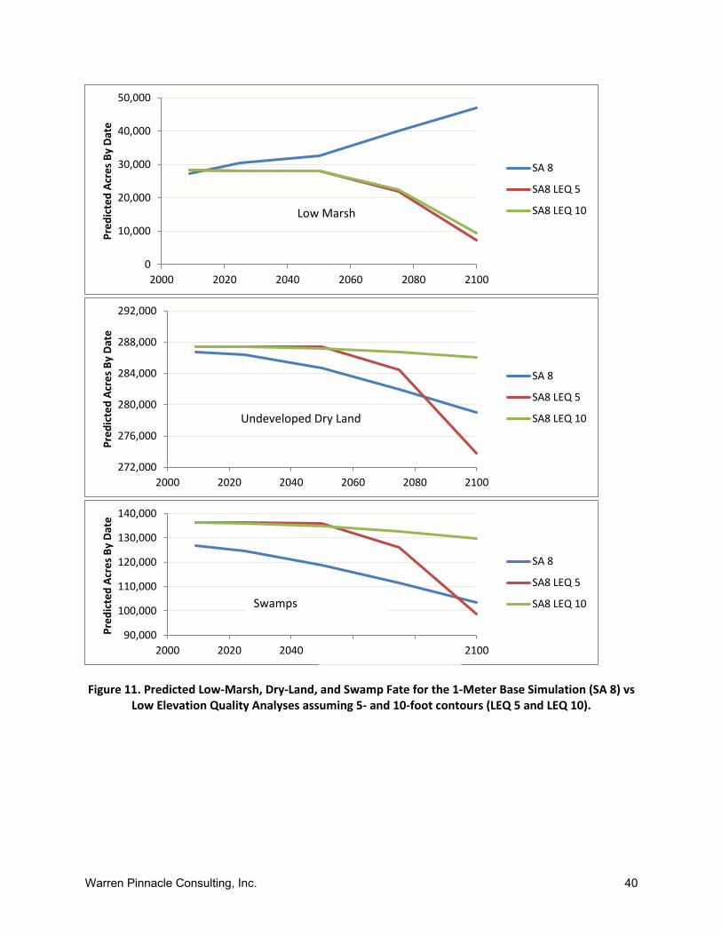
Warren Pinnacle Consulting, Inc. 40
Figure 11. Predicted Low-Marsh, Dry-Land, and Swamp Fate for the 1-Meter Base Simulation (SA 8) vs Low Elevation Quality Analyses assuming 5- and 10-foot contours (LEQ 5 and LEQ 10).
0
10,000
20,000
30,000
40,000
50,000
2000 2020 2040 2060 2080 2100
Pred
icte
d Ac
res B
y Da
te
SA 8
SA8 LEQ 5
SA8 LEQ 10
272,000
276,000
280,000
284,000
288,000
292,000
2000 2020 2040 2060 2080 2100
Pred
icte
d Ac
res B
y Da
te
SA 8
SA8 LEQ 5
SA8 LEQ 10
90,000
100,000
110,000
120,000
130,000
140,000
2000 2020 2040 2060 2080 2100
Pred
icte
d Ac
res B
y Da
te
SA 8
SA8 LEQ 5
SA8 LEQ 10Swamps
Low Marsh
Undeveloped Dry Land

Warren Pinnacle Consulting, Inc. 41
Figure 12. Comparison of Florida Site 8 (detail) Given Three Different Elevation Assumptions
Figure 12 shows an example of model predictions given the three different elevation data sets. These maps illustrate predictions in 2100 assuming 1-meter of SLR by that date. With LiDAR Data, currently-existing regularly-flooded marsh is expected to mostly persist and extensive migration into swamp lands is predicted. With 5-foot contours, most regularly-flooded marsh is predicted to be lost. Neighboring swamps have converted to transitional salt marsh but have not yet completed a transition to low marsh. With 10-foot contours, minimal conversion of neighboring swamp is predicted and nearly all regularly-flooded marsh is lost.
Results for the Texas site were similar if not more severe (Figure 13) as 5-meter contour data were generally not available in Texas, so this test was not run. However, the entire GCPLCC study area in
Undeveloped Dry Land Undeveloped Dry Land Cypress Swamp Cypress SwampOpen Ocean Open Ocean Trans. Salt Marsh Trans. Salt MarshSwamp Swamp Regularly-Flooded Marsh Regularly-Flooded Marsh
Area 8, Initial Condition Area 8, 2100, LiDAR Data 1 meter SLR by 2100
Area 8, 2100, 5 m Contours 1 meter SLR by 2100
Area 8, 2100, 10 m contours 1 meter SLR by 2100

Warren Pinnacle Consulting, Inc. 42
Texas was covered with LiDAR making this exercise largely academic and ultimately unimportant for the final results of this study.
Figure 13. Predicted Low-Marsh, Dry-Land, and Swamp Fate for the 1-Meter Base Simulation (SA 19) vs Low Elevation Quality Analysis 10-foot contours (LEQ 10).
0
10,000
20,000
30,000
40,000
50,000
60,000
70,000
2000 2020 2040 2060 2080 2100
Pred
icte
d Ac
res B
y Da
te
SA 19
SA 19 LEQ 10
600,000
605,000
610,000
615,000
620,000
625,000
2000 2020 2040 2060 2080 2100
Pred
icte
d Ac
res B
y Da
te
SA 19
SA 19 LEQ 10
21,000
21,500
22,000
22,500
23,000
23,500
24,000
2000 2020 2040 2060 2080 2100
Pred
icte
d Ac
res B
y Da
te
SA 19
SA 19 LEQ 10

Warren Pinnacle Consulting, Inc. 43
Conclusions and Perspectives This application of the SLAMM model and its associated focal-species analysis provides a Gulf-wide dataset to support conservation and adaptation strategies in the face of accelerated sea-level rise. This modeling effort used the best currently-available input data for both spatial and parametric inputs. However, results reported herein possess a level of uncertainty that must be kept in mind when interpreting them. Uncertainty in future rates of sea-level rise has been well addressed by considering a range of different scenarios. However, the uncertainty associated with the spatial and parametric data inputs have not been incorporated and the robustness of the predictions has not been assessed with respect to these uncertainties.
The current Gulf-wide model application assumes that marshes will successfully migrate into all (non-diked) dry lands regardless of their current use, development status, or likely future protection. As such, the model is informative in terms of potential future marsh habitats, but likely overstates future marsh resilience to sea-level rise, numerically. Evaluation of marsh-migration pathways in conjunction with likely future developed-land footprints (or a public vs. private-land overlay) may help to constrain model predictions.
Additional future analyses could incorporate linkage to salinity models (to further refine habitat switching assumptions), comparison to results from other models of marsh fate and migration, and refinements to the erosion and suspended sediment assumptions within the model. Updates to the SLAMM model could be directly applied to assess overall model uncertainty or to address the likelihood of SLR effects to development and transportation infrastructure. Storm-surge modeling can utilize future land-cover predictions to more accurately predict the effects of specific large storms.
The current Gulf-wide analysis is a large step forward in creating a seamless model that is consistent in model assumptions and accretion-feedback modeling. Hopefully this work will provide useful data for policymakers and planners for years to come, based both on current model outputs and through additional derived products.

Warren Pinnacle Consulting, Inc. 44
References Allen, J. A., Pezeshki, S. R., and Chambers, J. L. (1996). “Interaction of flooding and salinity stress
on baldcypress (Taxodium distichum).” Tree physiology, 16(1-2), 307. Cahoon, D. R., and Lynch, J. C. (1997). “Vertical accretion and shallow subsidence in a mangrove
forest of southwestern Florida, USA.” Mangroves and Salt Marshes, 1(3), 173–186. Cahoon, D. R., Reed, D. J., Day, J. W., and others. (1995). “Estimating shallow subsidence in
microtidal salt marshes of the southeastern United States: Kaye and Barghoorn revisited.” Marine Geology, 128(1-2), 1–9.
Callaway, J. C., DeLaune, R. D., and Patrick, Jr., W. H. (1997). “Sediment Accretion Rates from Four Coastal Wetlands along the Gulf of Mexico.” Journal of Coastal Research, 13(1), 181–191.
Chu-Agor, M. L., Munoz-Carpena, R., Kiker, G., Emanuelsson, A., and Linkov, I. (2010). “Global Sensitivity and Uncertainty Analysis of SLAMM for the Purpose of Habitat Vulnerability Assessment and Decision Making.”
Clough, J., Park, Richard, Marco, P., Polaczyk, A., and Fuller, R. (2012). “SLAMM 6.2 Technical Documentation.”
Couvillion, B. R., Barras, J. A., Steyer, G. D., Sleavin, William, Fischer, Michelle, Beck, Holly, Trahan, Nadine, Griffin, Brad, and Heckman, David. (2011). Land area change in coastal Louisiana from 1932 to 2010: U.S. Geological Survey Scientific Investigations Map 3164, scale 1:265,000. pamphlet, 12.
Craft, C., Clough, J. S., Ehman, J., Joye, S., Park, R. A., Pennings, S., Guo, H., and Machmuller, M. (2009). “Forecasting the effects of accelerated sea-level rise on tidal marsh ecosystem services.” Frontiers in Ecology and the Environment, 7(2), 73–78.
DeLaune, R. D., Whitcomb, J. H., Patrick, W. H., Pardue, J. H., and Pezeshki, S. R. (1989). “Accretion and canal impacts in a rapidly subsiding wetland. I. 137Cs and210Pb techniques.” Estuaries, 12(4), 247–259.
Donoghue, J. (2011). “SET question.” Fry, J., Xian, G., Jin, S., Dewitz, J., Homer, C., Yang, L., Barnes, C., Herold, N., and Wickham, J.
(2011). “Completion of the 2006 National Land Cover Database for the Conterminous United States, PE&RS, Vol. 77 (9): 858-864.” Websites: http://www. mrlc. gov/nlcd2006. php, and http://www. mrlc. gov/downloadfile2. php.
Galbraith, H., Jones, R., Park, R., Clough, J., Herrod-Julius, S., Harrington, B., and Page, G. (2002). “Global Climate Change and Sea Level Rise: Potential Losses of Intertidal Habitat for Shorebirds.” Waterbirds, 25(2), 173.
Glick, P., Clough, J., and Nunley, B. (2007). Sea-level Rise and Coastal Habitats in the Pacific Northwest: An Analysis for Puget Sound, Southwestern Washington, and Northwestern Oregon. National Wildlife Federation.
Glick, P., Clough, J., Polaczyk, A., Couvillion, B., and Nunley, B. (2013). “Potential Effects of Sea-Level Rise on Coastal Wetlands in Southeastern Louisiana.” Journal of Coastal Research, 63(sp1), 211–233.
Glick, P., Clough, J., Polaczyk, A., and Nunley, B. (2011). Sea-Level Rise and Coastal Habitats in Southeastern Louisiana: An Application of the Sea Level Affecting Marshes (SLAMM) Model. Draft Technical Report. National Wildlife Federation.

Warren Pinnacle Consulting, Inc. 45
Hendrickson, J. C. (1997). “Coastal wetland response to rising sea-level: quantification of short-and long-term accretion and subsidence, northeastern Gulf of Mexico.” Florida State University, Tallahassee, FL.
Keeland, B. D., Conner, W. H., and Sharitz, R. R. (1997). “A comparison of wetland tree growth response to hydrologic regime in Louisiana and South Carolina.” Forest ecology and management, 90(2-3), 237–250.
Kirwan, M. L., Guntenspergen, G. R., D’Alpaos, A., Morris, J. T., Mudd, S. M., and Temmerman, S. (2010). “Limits on the adaptability of coastal marshes to rising sea level.” Geophysical Research Letters, 37(23).
McKee, K. L. (2011). “Biophysical controls on accretion and elevation change in Caribbean mangrove ecosystems.” Estuarine, Coastal and Shelf Science, 91(4), 475–483.
McKee, K., and Patrick. (1988). “The Relationship of Smooth Cordgrass (Spartina alterniflora) to Tidal Datums: A Review.” Estuaries, 11(3), 143–151.
Mcleod, E., Poulter, B., Hinkel, J., Reyes, E., and Salm, R. (2010). “Sea-level rise impact models and environmental conservation: A review of models and their applications.” Ocean & Coastal Management, 53(9), 507–517.
Morris, J. (2013). “Marsh Equilibrium Model–Version 3.4.” Morris, J. T., Edwards, J., Crooks, S., and Reyes, E. (2012). “Assessment of carbon sequestration
potential in coastal wetlands.” Recarbonization of the Biosphere, Springer, 517–531. Morris, J. T., Sundareshwar, P. V., Nietch, C. T., Kjerfve, B., and Cahoon, D. R. (2002). “Responses
of coastal wetlands to rising sea level.” Ecology, 83(10), 2869–2877. National Wildlife Federation, and Florida Wildlife Federation. (2006). An Unfavorable Tide: Global
Warming, Coastal Habitats and Sportfishing in Florida. NOS. (2013). VDATUM. Nyman, J. A., DeLaune, R. D., Roberts, H. H., and Patrick Jr, W. H. (1993). “Relationship between
vegetation and soil formation in a rapidly submerging coastal marsh.” Marine ecology progress series. Oldendorf, 96(3), 269–279.
Osland, M. J., Enwright, N., Day, R. H., and Doyle, T. W. (2013). “Winter climate change and coastal wetland foundation species: salt marshes vs. mangrove forests in the southeastern United States.” Global change biology, 19(5), 1482–1494.
Park, R. A., Lee, J. K., and Canning, D. J. (1993). “Potential Effects of Sea-Level Rise on Puget Sound Wetlands.” Geocarto International, 8(4), 99.
Park, R. A., Lee, J. K., Mausel, P. W., and Howe, R. C. (1991). “Using remote sensing for modeling the impacts of sea level rise.” World Resources Review, 3, 184–220.
Park, R. A., Trehan, M. S., Mausel, P. W., and Howe, R. C. (1989). “The Effects of Sea Level Rise on U.S. Coastal Wetlands.” The Potential Effects of Global Climate Change on the United States: Appendix B - Sea Level Rise, U.S. Environmental Protection Agency, Washington, DC, 1–1 to 1–55.
Radosavljevic, B., Gibeaut, J., and Tissot, P. (2012). “Sea-Level Rise: Estuarine Wetlands of Mustang Island at Imminent Risk of Submergence.” EGU General Assembly Conference Abstracts, 6554.
Reed, D. J. (1995). “The response of coastal marshes to sea-level rise: Survival or submergence?” Earth Surface Processes and Landforms, 20(1), 39–48.
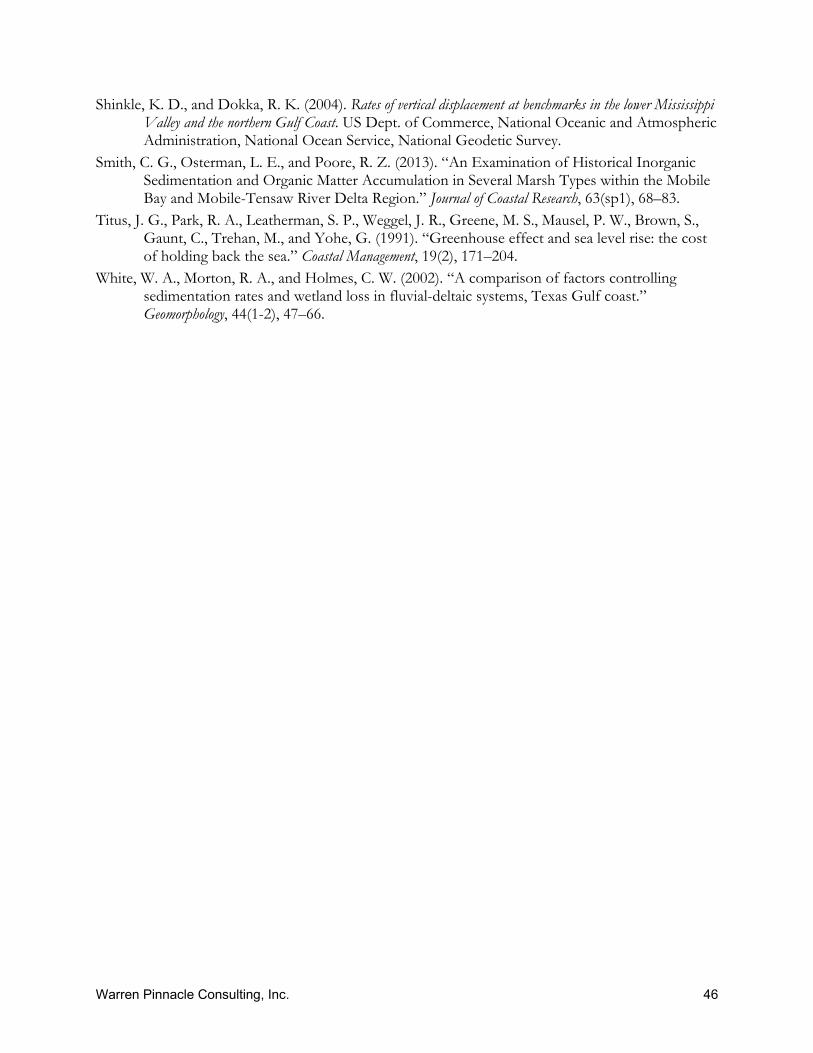
Warren Pinnacle Consulting, Inc. 46
Shinkle, K. D., and Dokka, R. K. (2004). Rates of vertical displacement at benchmarks in the lower Mississippi Valley and the northern Gulf Coast. US Dept. of Commerce, National Oceanic and Atmospheric Administration, National Ocean Service, National Geodetic Survey.
Smith, C. G., Osterman, L. E., and Poore, R. Z. (2013). “An Examination of Historical Inorganic Sedimentation and Organic Matter Accumulation in Several Marsh Types within the Mobile Bay and Mobile-Tensaw River Delta Region.” Journal of Coastal Research, 63(sp1), 68–83.
Titus, J. G., Park, R. A., Leatherman, S. P., Weggel, J. R., Greene, M. S., Mausel, P. W., Brown, S., Gaunt, C., Trehan, M., and Yohe, G. (1991). “Greenhouse effect and sea level rise: the cost of holding back the sea.” Coastal Management, 19(2), 171–204.
White, W. A., Morton, R. A., and Holmes, C. W. (2002). “A comparison of factors controlling sedimentation rates and wetland loss in fluvial-deltaic systems, Texas Gulf coast.” Geomorphology, 44(1-2), 47–66.

Data Source, YearNOAA Digital Coast, 2004 - 2008National Elevation Data Set 1/3rd arc second data, 1999National Elevation Dataset 1/9th arcsecond, 2007
Study Area 1 DEM Sources
Warren Pinnacle Consulting, Inc. A-1

Study Area 2 DEM Sources
Data Source, YearNOAA Digital Coast, 2004 - 2008National Elevation Dataset 1/3rd arcsecond, 1999National Elevation Dataset 1/9th arcsecond, 2007 - 2008
Warren Pinnacle Consulting, Inc. A-2
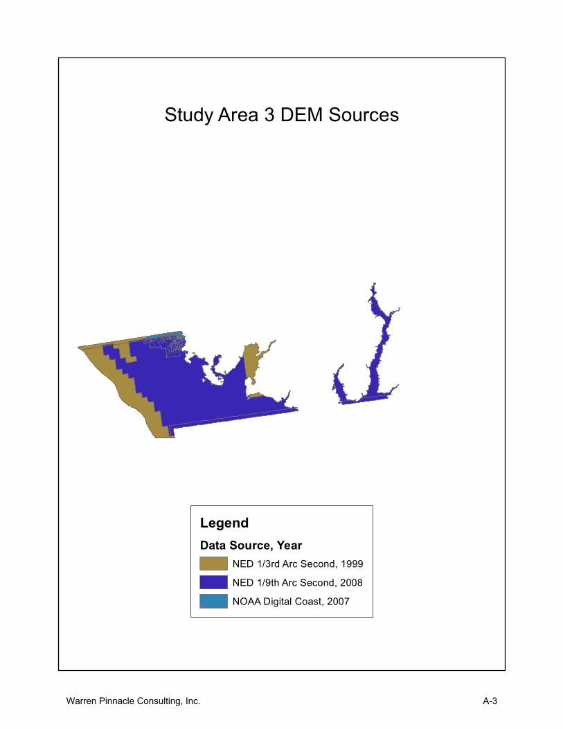
Study Area 3 DEM Sources
LegendData Source, Year
NED 1/3rd Arc Second, 1999NED 1/9th Arc Second, 2008NOAA Digital Coast, 2007
Warren Pinnacle Consulting, Inc. A-3

Study Area 4, Elevation Data Sources
Data SourceNational Elevation Dataset 1/9th arcsecond, 2007
Warren Pinnacle Consulting, Inc. A-4

Study Area 5 DEM Sources
National Elevation Dataset 1/9th arcsecond, 2009
Warren Pinnacle Consulting, Inc. A-5
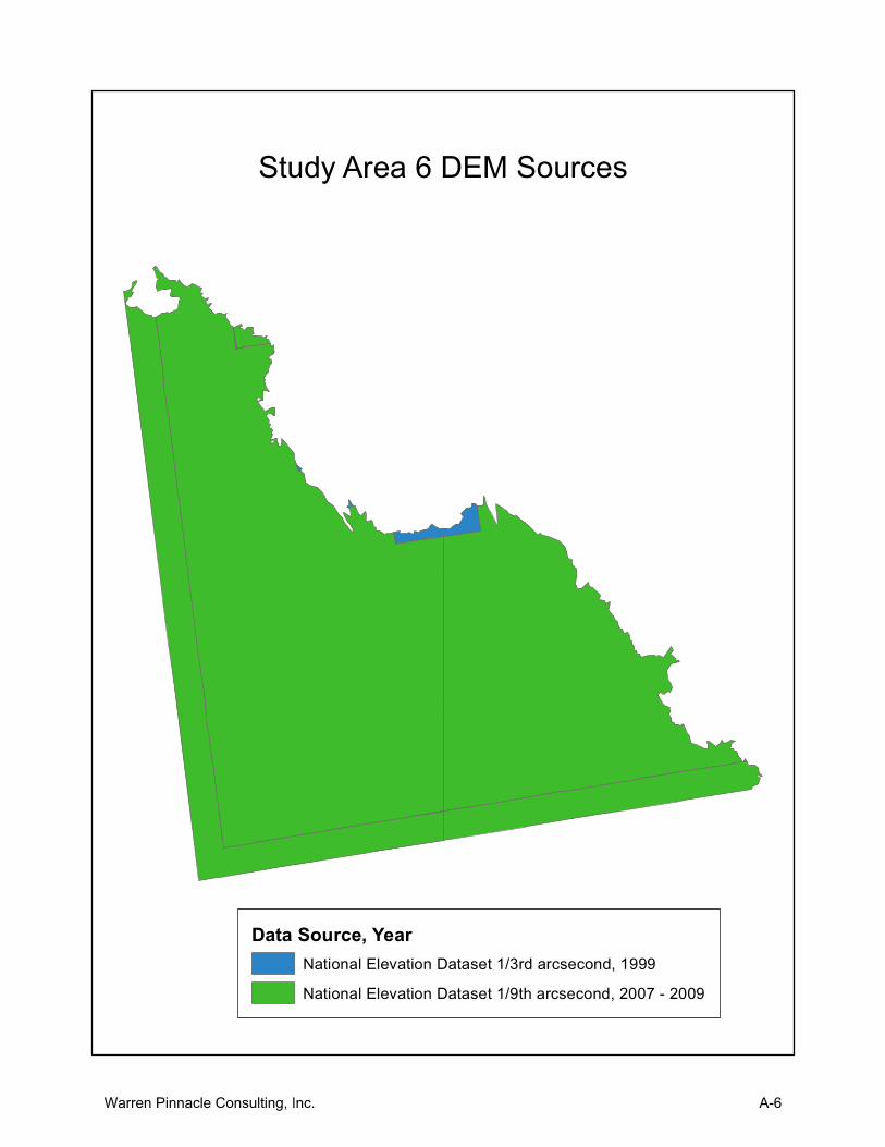
Data Source, YearNational Elevation Dataset 1/3rd arcsecond, 1999National Elevation Dataset 1/9th arcsecond, 2007 - 2009
Study Area 6 DEM Sources
Warren Pinnacle Consulting, Inc. A-6

Study Area 7 DEM Sources
Data SourceNOAA Digital Coast, 2008National Elevation Dataset 1/9th arcsecond, 2008
Warren Pinnacle Consulting, Inc. A-7

Study Area 8 DEM Sources
Data Source, YearNOAA Digital Coast, 2009National Elevation Dataset 1/3rd arcsecond, 1999National Elevation Dataset 1/9th arcsecond, 2009
Warren Pinnacle Consulting, Inc. A-8

Study Area 9 DEM Sources
Data Source, YearNOAA Digital Coast, 2007National Elevation Dataset 1/3rd arcsecond, 1999National Elevation Dataset 1/9th arcsecond, 2009
Warren Pinnacle Consulting, Inc. A-9

Study Area 10 DEM Sources
Data Source, YearNational Elevation Dataset 1/9th arcsecond, 2007 - 2009
Warren Pinnacle Consulting, Inc. A-10

Study Area 11 DEM Sources
Data Source, YearNED 1/9th ArcSecond, 2009
Warren Pinnacle Consulting, Inc. A-11

Study Area 12 DEM Sources
Data Source, YearNED 1/3rd ArcSecond, 1999NED 1/9th ArcSecond, 2009
Warren Pinnacle Consulting, Inc. A-12
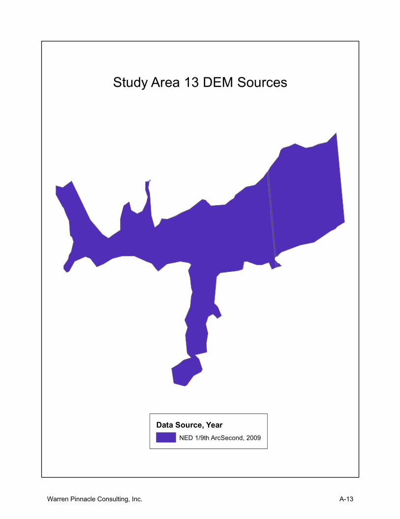
Study Area 13 DEM Sources
Data Source, YearNED 1/9th ArcSecond, 2009
Warren Pinnacle Consulting, Inc. A-13

Study Area 14 DEM Sources
Data Sources, YearNED 1/3rd ArcSecond, 1999NED 1/9th ArcSecond, 2007 - 2009NOAA Digital Coast, 2004 - 2008
Warren Pinnacle Consulting, Inc. A-14

Study Area 16, Elevation Source Date
Data SourceNational Elevation Dataset 1/3rd arcsecond, 1999
Warren Pinnacle Consulting, Inc. A-15

Study Area 17 DEM Sources
Data Source, YearNED 1/3rd ArcSecond, 1999NED 1/9th ArcSecond, 2007
Warren Pinnacle Consulting, Inc. A-16

Study Area 18 DEM Sources
Data Source, YearNED 1/9th ArcSecond, 2009NOAA Digital Coast, 2008
Warren Pinnacle Consulting, Inc. A-17

Study Area 19 DEM Sources
Data Source, YearNED 1/3rd arc second, 1999NED 1/9th arc second, 2009
Warren Pinnacle Consulting, Inc. A-18
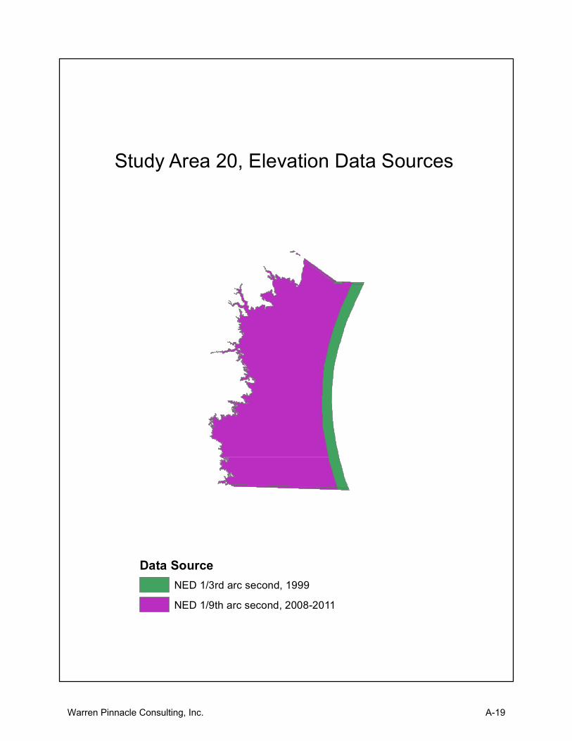
Study Area 20, Elevation Data Sources
Data SourceNED 1/3rd arc second, 1999NED 1/9th arc second, 2008-2011
Warren Pinnacle Consulting, Inc. A-19
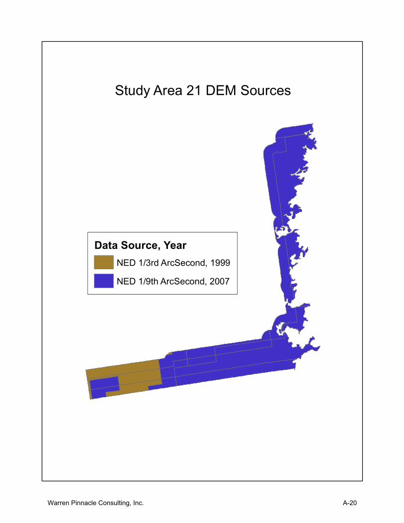
Study Area 21 DEM Sources
Data Source, YearNED 1/3rd ArcSecond, 1999NED 1/9th ArcSecond, 2007
Warren Pinnacle Consulting, Inc. A-20
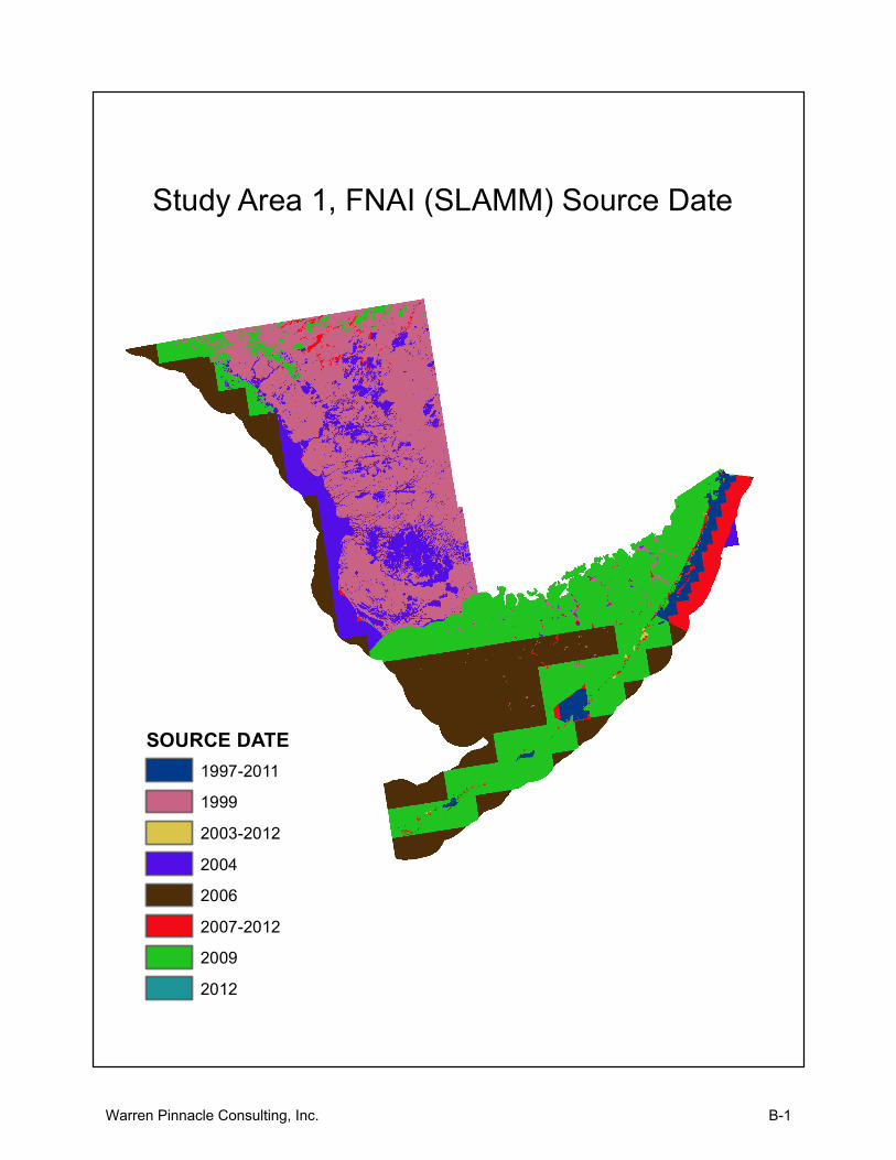
Study Area 1, FNAI (SLAMM) Source Date
SOURCE DATE1997-201119992003-2012200420062007-201220092012
Warren Pinnacle Consulting, Inc. B-1

Study Area 2, FNAI (SLAMM) Source Date
SOURCE DATE1997-201119992001-20122003-20122004-200620062007-201220092011
Warren Pinnacle Consulting, Inc. B-2

Study Area 3, FNAI (SLAMM) Source Date
SOURCE DATE1997-20112001-20112001-20122003-201220062007-201220092011
Warren Pinnacle Consulting, Inc. B-3
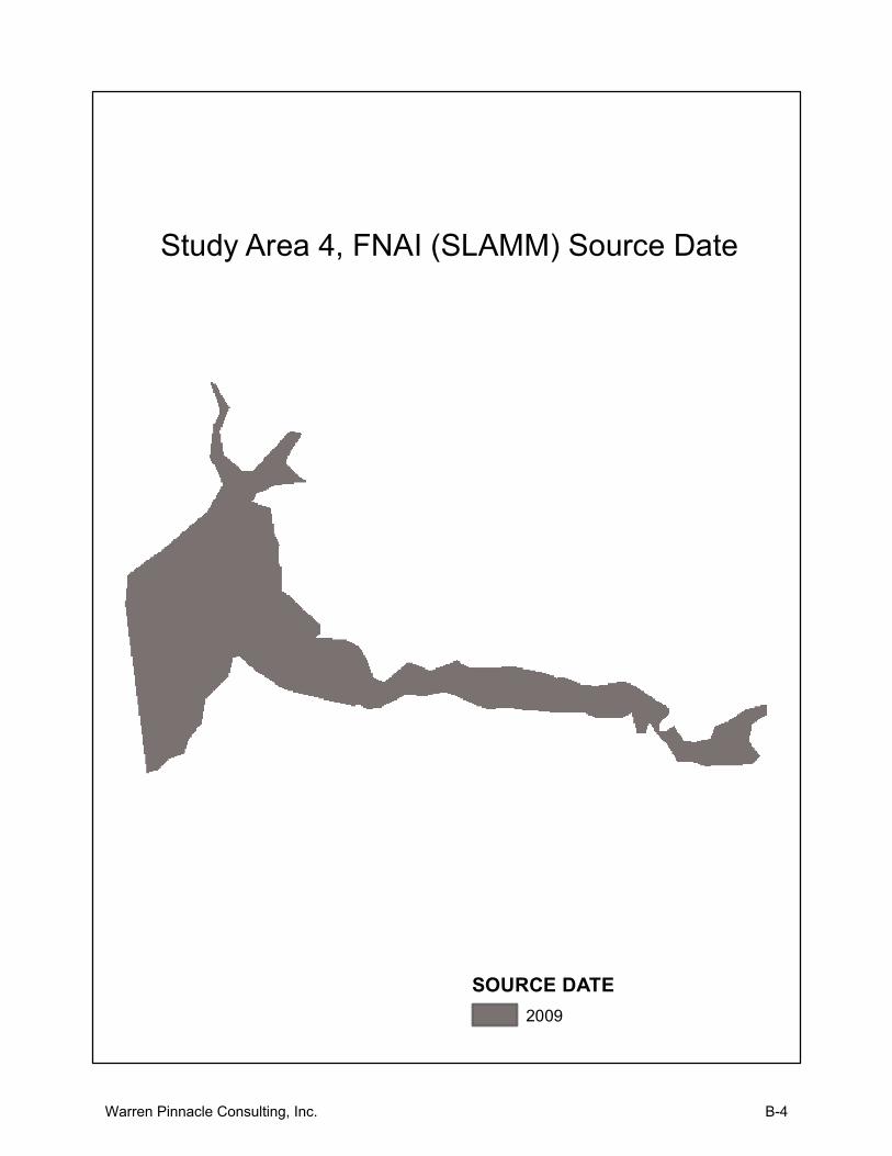
Study Area 4, FNAI (SLAMM) Source Date
SOURCE DATE2009
Warren Pinnacle Consulting, Inc. B-4
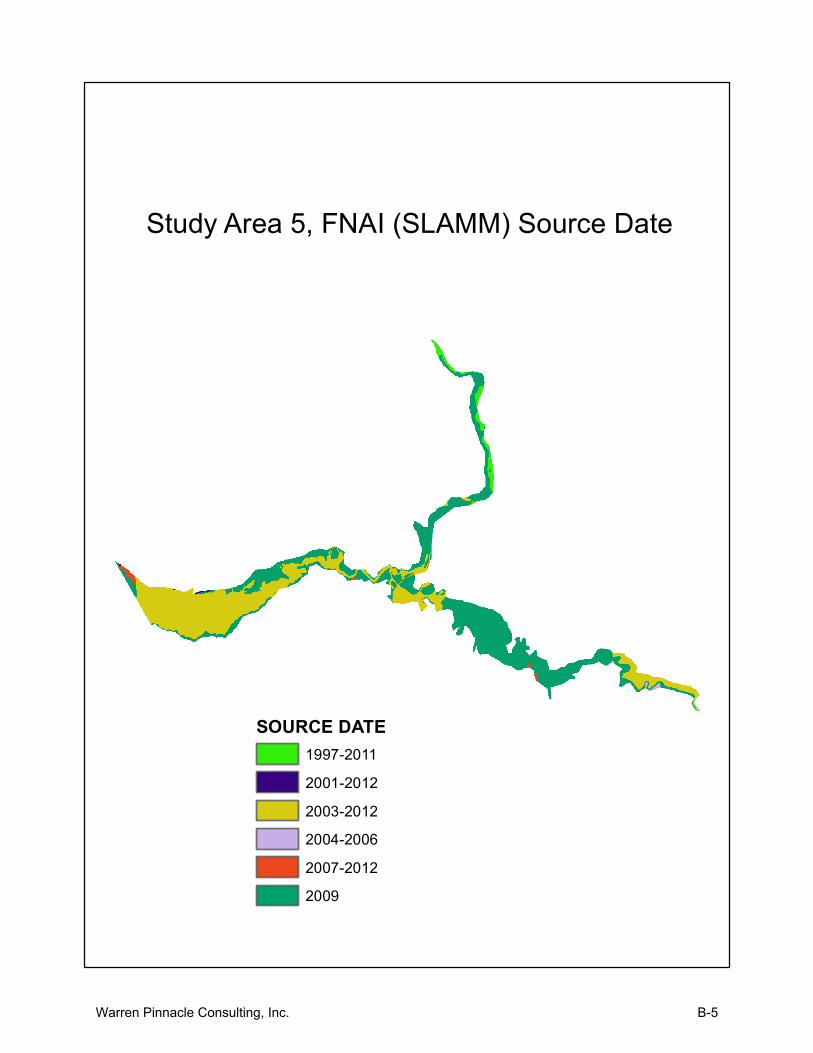
Study Area 5, FNAI (SLAMM) Source Date
SOURCE DATE1997-20112001-20122003-20122004-20062007-20122009
Warren Pinnacle Consulting, Inc. B-5

Study Area 6, FNAI (SLAMM) Source Date
SOURCE DATE2004-20062007-20122009
Warren Pinnacle Consulting, Inc. B-6
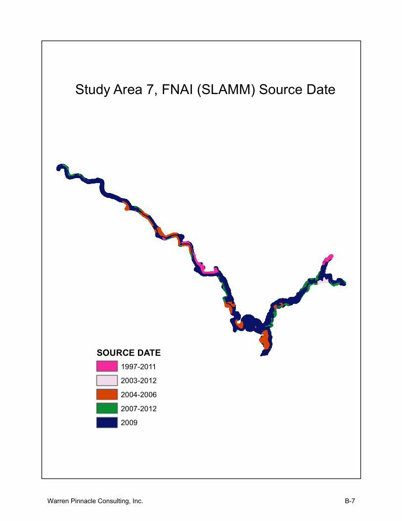
Study Area 7, FNAI (SLAMM) Source Date
SOURCE DATE1997-20112003-20122004-20062007-20122009
Warren Pinnacle Consulting, Inc. B-7

Study Area 8, FNAI (SLAMM) Source Date
SOURCEDATE1997-20112001-20122003-20122004-200620062007-20122009
Warren Pinnacle Consulting, Inc. B-8

Study Area 9, FNAI (SLAMM) Source Date
SOURCE DATE2001-20122003-20122004-200620062007-201220092011
Warren Pinnacle Consulting, Inc. B-9
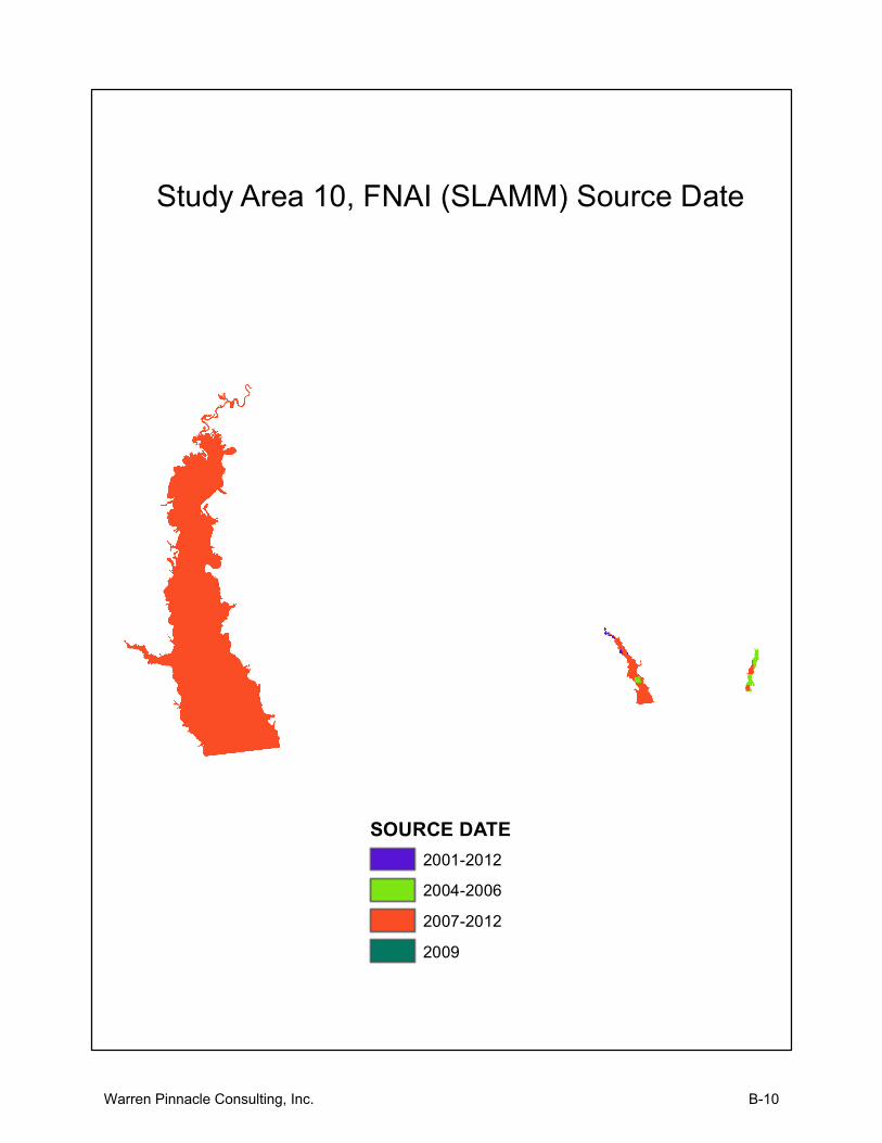
Study Area 10, FNAI (SLAMM) Source Date
SOURCE DATE2001-20122004-20062007-20122009
Warren Pinnacle Consulting, Inc. B-10

Study Area 11, NWI (SLAMM) Source Date
Source Date2001
Warren Pinnacle Consulting, Inc. B-11

Study Area 12, NWI (SLAMM) Source Date
Source Date1980198119822001
Warren Pinnacle Consulting, Inc. B-12

Study Area 13, NWI (SLAMM) Source Date
Source Date2001
Warren Pinnacle Consulting, Inc. B-13

Study Area 14, NWI (SLAMM) Source Date
Source Date19801981200220072010
Warren Pinnacle Consulting, Inc. B-14
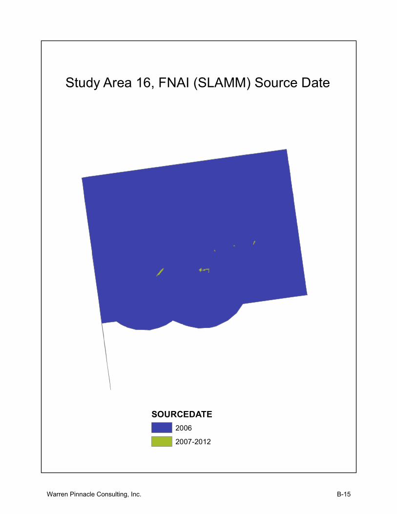
Study Area 16, FNAI (SLAMM) Source Date
SOURCEDATE20062007-2012
Warren Pinnacle Consulting, Inc. B-15

Study Area 17, NWI/NGOM (SLAMM) Source Date
NGOMSource Date
2008NWISource Date
1982198819891992199319942006
Warren Pinnacle Consulting, Inc. B-16
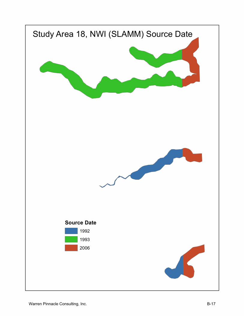
Study Area 18, NWI (SLAMM) Source Date
Source Date199219932006
Warren Pinnacle Consulting, Inc. B-17

Study Area 19, NWI (SLAMM) Source Date
Source Date1992200120062008
Warren Pinnacle Consulting, Inc. B-18

Study Area 20, NWI (SLAMM) Source Date
Source DateUnknown199219942006
Warren Pinnacle Consulting, Inc. B-19

Warren Pinnacle Consulting, Inc. C-1
Appendix C – Parameters for New Study Areas
Parameter Unit/Format
NWI Photo Date YYYY
DEM Date YYYY
Direction Offshore n,s,e,w
Historic Trend mm/yr
Historic Eustatic Trend mm/yr
MTL-NAVD88 m
GT - Great Diurnal Tide Range m
Salt Elev. m above MTL
Marsh Erosion horz. m /yr
Swamp Erosion horz. m /yr
T.Flat Erosion horz. m /yr
Reg.-Flood Marsh Accr mm/yr
Irreg.-Flood Marsh Accr mm/yr
Tidal-Fresh Marsh Accr mm/yr
Inland-Fresh Marsh Accr mm/yr
Mangrove Accr mm/yr
Tidal Swamp Accr mm/yr
Swamp Accretion mm/yr
Beach Sed. Rate mm/yr
Freq. Overwash years
Use Elev Pre-processor True,False
Reg Flood Max. Accr. mm/yr
Reg Flood Min. Accr. mm/yr
Reg Flood Elev a mm/year*HTU^3
Reg Flood Elev b mm/year*HTU^2
Reg Flood Elev c mm/year*HTU
Reg Flood Elev d mm/yr
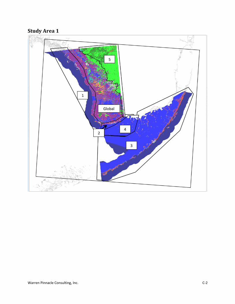
Warren Pinnacle Consulting, Inc. C-2
Study Area 1
Global
1
2
3
4
5

Warren Pinnacle Consulting, Inc. C-3
Parameter Global SubSite 1 SubSite 2 SubSite 3 SubSite 4 SubSite 5
Description Interior tides Gulf tides South Gulf
Tides Keys South Gulf Tides 2009
Interior tides DEM
1999 NWI Photo Date 1999 1999 1999 2009 2009 1999 DEM Date 2007 2007 2007 2007 1999 1999 Direction Offshore West West South South West West Historic Trend 2.4 2.4 2.78 2.78 2.78 2.4 Historic Eustatic Trend 1.7 1.7 1.7 1.7 1.7 1.7 MTL-NAVD88 0 0 0 0 0 0 GT 0.244 1.3 0.77 0.44 0.77 0.244 Salt Elev. 0.371 0.967 0.668 0.48 0.668 0.371 Marsh Erosion 0 0 0 0 0 0 Swamp Erosion 0 0 0 0 0 0 T.Flat Erosion 0 0 0 0 0 0 Reg.-Flood Marsh Accr 0 0 0 0 0 0 Irreg.-Flood Marsh Accr 4.7 4.7 4.7 4.7 4.7 4.7 Tidal-Fresh Marsh Accr 5.9 5.9 5.9 5.9 5.9 5.9 Inland-Fresh Marsh Accr 5.9 5.9 5.9 5.9 5.9 5.9 Mangrove Accr 2 2 2 2 2 2 Tidal Swamp Accr 1.1 1.1 1.1 1.1 1.1 1.1 Swamp Accretion 0.3 0.3 0.3 0.3 0.3 0.3 Beach Sed. Rate 0.75 0.75 0.75 0.75 0.75 0.75 Freq. Overwash 0 0 0 0 0 0 Use Elev Pre-processor FALSE FALSE FALSE FALSE TRUE TRUE Reg Flood Max. Accr. 4.9 4.9 4.9 4.9 4.9 4.9 Reg Flood Min. Accr. 0.8 0.8 0.8 0.8 0.8 0.8 Reg Flood Elev a 4.905004 4.905004 4.905004 4.905004 4.905004 4.905004 Reg Flood Elev b -8.36954 -8.36954 -8.36954 -8.36954 -8.36954 -8.36954
Reg Flood Elev c -1.88503 -1.88503 -1.88503 -1.88503 -1.88503 -1.88503
Reg Flood Elev d 6.54377 6.54377 6.54377 6.54377 6.54377 6.54377
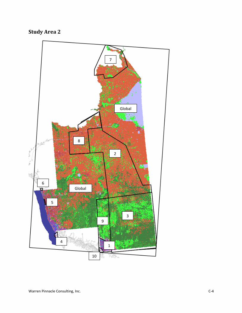
Warren Pinnacle Consulting, Inc. C-4
Study Area 2
1
Global
2
3
4
5
6
7
8
9
10
Global
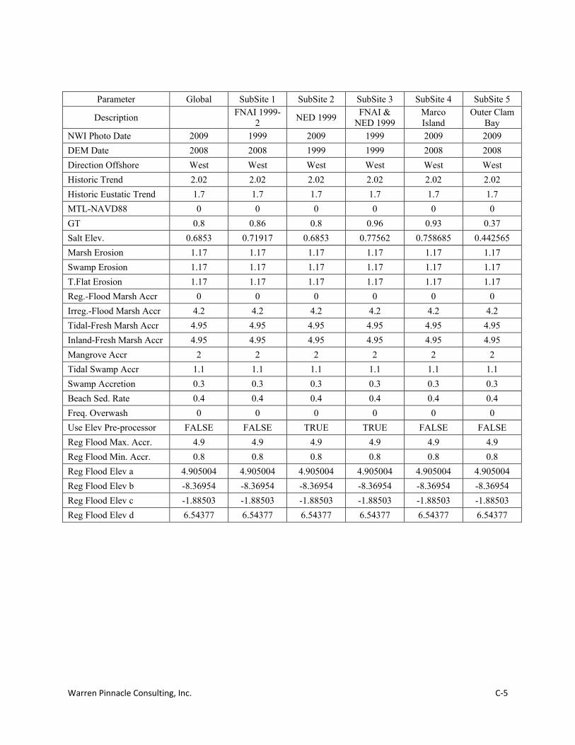
Warren Pinnacle Consulting, Inc. C-5
Parameter Global SubSite 1 SubSite 2 SubSite 3 SubSite 4 SubSite 5
Description FNAI 1999-
2 NED 1999 FNAI & NED 1999
Marco Island
Outer Clam Bay
NWI Photo Date 2009 1999 2009 1999 2009 2009 DEM Date 2008 2008 1999 1999 2008 2008 Direction Offshore West West West West West West Historic Trend 2.02 2.02 2.02 2.02 2.02 2.02 Historic Eustatic Trend 1.7 1.7 1.7 1.7 1.7 1.7 MTL-NAVD88 0 0 0 0 0 0 GT 0.8 0.86 0.8 0.96 0.93 0.37 Salt Elev. 0.6853 0.71917 0.6853 0.77562 0.758685 0.442565 Marsh Erosion 1.17 1.17 1.17 1.17 1.17 1.17 Swamp Erosion 1.17 1.17 1.17 1.17 1.17 1.17 T.Flat Erosion 1.17 1.17 1.17 1.17 1.17 1.17 Reg.-Flood Marsh Accr 0 0 0 0 0 0 Irreg.-Flood Marsh Accr 4.2 4.2 4.2 4.2 4.2 4.2 Tidal-Fresh Marsh Accr 4.95 4.95 4.95 4.95 4.95 4.95 Inland-Fresh Marsh Accr 4.95 4.95 4.95 4.95 4.95 4.95 Mangrove Accr 2 2 2 2 2 2 Tidal Swamp Accr 1.1 1.1 1.1 1.1 1.1 1.1 Swamp Accretion 0.3 0.3 0.3 0.3 0.3 0.3 Beach Sed. Rate 0.4 0.4 0.4 0.4 0.4 0.4 Freq. Overwash 0 0 0 0 0 0 Use Elev Pre-processor FALSE FALSE TRUE TRUE FALSE FALSE Reg Flood Max. Accr. 4.9 4.9 4.9 4.9 4.9 4.9 Reg Flood Min. Accr. 0.8 0.8 0.8 0.8 0.8 0.8 Reg Flood Elev a 4.905004 4.905004 4.905004 4.905004 4.905004 4.905004 Reg Flood Elev b -8.36954 -8.36954 -8.36954 -8.36954 -8.36954 -8.36954 Reg Flood Elev c -1.88503 -1.88503 -1.88503 -1.88503 -1.88503 -1.88503 Reg Flood Elev d 6.54377 6.54377 6.54377 6.54377 6.54377 6.54377

Warren Pinnacle Consulting, Inc. C-6
Parameter SubSite 6 SubSite 7 SubSite 8 SubSite 9 SubSite 10
Description little Hickory Bay SubSite 7 SubSite 8 FNAI 1999
muted tide FNAI 1999-1
NWI Photo Date 2009 2009 2009 1999 2009 DEM Date 2008 1999 2008 2008 2008 Direction Offshore West West West West West Historic Trend 2.02 2.02 2.02 2.02 2.02 Historic Eustatic Trend 1.7 1.7 1.7 1.7 1.7 MTL-NAVD88 0 0 0 0 0 GT 0.28 0.8 0.8 0.4 0.96 Salt Elev. 0.39176 0.6853 0.6853 0.4595 0.77562 Marsh Erosion 1.17 1.17 1.17 1.17 1.17 Swamp Erosion 1.17 1.17 1.17 1.17 1.17 T.Flat Erosion 1.17 1.17 1.17 1.17 1.17 Reg.-Flood Marsh Accr 0 0 0 0 0 Irreg.-Flood Marsh Accr 4.2 4.2 4.2 4.2 4.2
Tidal-Fresh Marsh Accr 4.95 4.95 4.95 4.95 4.95 Inland-Fresh Marsh Accr 4.95 4.95 4.95 4.95 4.95
Mangrove Accr 2 2 2 2 2 Tidal Swamp Accr 1.1 1.1 1.1 1.1 1.1 Swamp Accretion 0.3 0.3 0.3 0.3 0.3 Beach Sed. Rate 0.4 0.4 0.4 0.4 0.4 Freq. Overwash 0 0 0 0 0 Use Elev Pre-processor FALSE FALSE FALSE FALSE FALSE Reg Flood Max. Accr. 4.9 4.9 4.9 4.9 4.9 Reg Flood Min. Accr. 0.8 0.8 0.8 0.8 0.8 Reg Flood Elev a 4.905004 4.905004 4.905004 4.905004 4.905004 Reg Flood Elev b -8.36954 -8.36954 -8.36954 -8.36954 -8.36954 Reg Flood Elev c -1.88503 -1.88503 -1.88503 -1.88503 -1.88503 Reg Flood Elev d 6.54377 6.54377 6.54377 6.54377 6.54377

Warren Pinnacle Consulting, Inc. C-7
Study Area 3
Global
1
2 3

Warren Pinnacle Consulting, Inc. C-8
Parameter Global SubSite 1 SubSite 2 SubSite 3
Description SubSite 1 SubSite 2 Global North
NWI Photo Date 2009 2009 2009 2009 DEM Date 2008 2008 1999 2008 Direction Offshore East South East East Historic Trend 2.4 2.4 2.4 2.4 Historic Eustatic Trend 1.7 1.7 1.7 1.7 MTL-NAVD88 0 -0.14 0 0 GT 0.53 0.66 0.63 0.63 Salt Elev. 0.533 0.606 0.589 0.589 Marsh Erosion 1 1 1 1 Swamp Erosion 1 1 1 1 T.Flat Erosion 1 1 1 1 Reg.-Flood Marsh Accr 0 0 0 0 Irreg.-Flood Marsh Accr 3.75 3.75 3.75 3.75 Tidal-Fresh Marsh Accr 4 4 4 4 Inland-Fresh Marsh Accr 4 4 4 4 Mangrove Accr 2 2 2 2 Tidal Swamp Accr 1.1 1.1 1.1 1.1 Swamp Accretion 0.3 0.3 0.3 0.3 Beach Sed. Rate 0.5 0.5 0.5 0.5 Freq. Overwash 25 25 25 25 Use Elev Pre-processor FALSE FALSE TRUE FALSE Reg Flood Max. Accr. 4.9 4.9 4.9 4.9 Reg Flood Min. Accr. 0.8 0.8 0.8 0.8 Reg Flood Elev a 4.905004 4.905004 4.905004 4.905004 Reg Flood Elev b -8.36954 -8.36954 -8.36954 -8.36954 Reg Flood Elev c -1.88503 -1.88503 -1.88503 -1.88503 Reg Flood Elev d 6.54377 6.54377 6.54377 6.54377
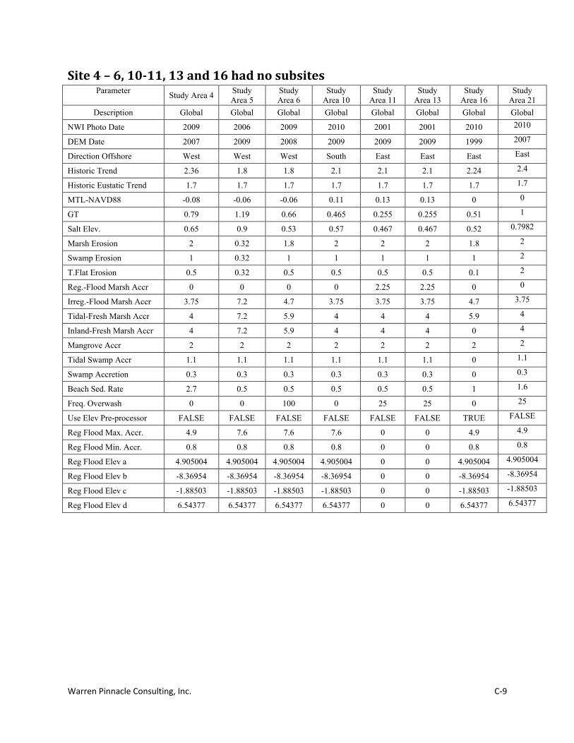
Warren Pinnacle Consulting, Inc. C-9
Site 4 – 6, 10-11, 13 and 16 had no subsites Parameter Study Area 4 Study
Area 5 Study Area 6
Study Area 10
Study Area 11
Study Area 13
Study Area 16
Study Area 21
Description Global Global Global Global Global Global Global Global
NWI Photo Date 2009 2006 2009 2010 2001 2001 2010 2010
DEM Date 2007 2009 2008 2009 2009 2009 1999 2007
Direction Offshore West West West South East East East East
Historic Trend 2.36 1.8 1.8 2.1 2.1 2.1 2.24 2.4
Historic Eustatic Trend 1.7 1.7 1.7 1.7 1.7 1.7 1.7 1.7
MTL-NAVD88 -0.08 -0.06 -0.06 0.11 0.13 0.13 0 0
GT 0.79 1.19 0.66 0.465 0.255 0.255 0.51 1
Salt Elev. 0.65 0.9 0.53 0.57 0.467 0.467 0.52 0.7982
Marsh Erosion 2 0.32 1.8 2 2 2 1.8 2
Swamp Erosion 1 0.32 1 1 1 1 1 2
T.Flat Erosion 0.5 0.32 0.5 0.5 0.5 0.5 0.1 2
Reg.-Flood Marsh Accr 0 0 0 0 2.25 2.25 0 0
Irreg.-Flood Marsh Accr 3.75 7.2 4.7 3.75 3.75 3.75 4.7 3.75
Tidal-Fresh Marsh Accr 4 7.2 5.9 4 4 4 5.9 4
Inland-Fresh Marsh Accr 4 7.2 5.9 4 4 4 0 4
Mangrove Accr 2 2 2 2 2 2 2 2
Tidal Swamp Accr 1.1 1.1 1.1 1.1 1.1 1.1 0 1.1
Swamp Accretion 0.3 0.3 0.3 0.3 0.3 0.3 0 0.3
Beach Sed. Rate 2.7 0.5 0.5 0.5 0.5 0.5 1 1.6
Freq. Overwash 0 0 100 0 25 25 0 25
Use Elev Pre-processor FALSE FALSE FALSE FALSE FALSE FALSE TRUE FALSE
Reg Flood Max. Accr. 4.9 7.6 7.6 7.6 0 0 4.9 4.9
Reg Flood Min. Accr. 0.8 0.8 0.8 0.8 0 0 0.8 0.8
Reg Flood Elev a 4.905004 4.905004 4.905004 4.905004 0 0 4.905004 4.905004
Reg Flood Elev b -8.36954 -8.36954 -8.36954 -8.36954 0 0 -8.36954 -8.36954
Reg Flood Elev c -1.88503 -1.88503 -1.88503 -1.88503 0 0 -1.88503 -1.88503
Reg Flood Elev d 6.54377 6.54377 6.54377 6.54377 0 0 6.54377 6.54377

Warren Pinnacle Consulting, Inc. C-10
Study Area 7
Global
1

Warren Pinnacle Consulting, Inc. C-11
Parameter Global SubSite 1 Description 1/3 arcsecond
NWI Photo Date 2007 2007 DEM Date 2009 2009 Direction Offshore South South Historic Trend 1.8 1.8 Historic Eustatic Trend 1.7 1.7 MTL-NAVD88 0.18 0.18 GT 0.6584 0.6584 Salt Elev. 0.5334 0.5334 Marsh Erosion 1.8 1.8 Swamp Erosion 1 1 T.Flat Erosion 0.5 0.5 Reg.-Flood Marsh Accr 0 0 Irreg.-Flood Marsh Accr 4.7 4.7 Tidal-Fresh Marsh Accr 5.9 5.9 Inland-Fresh Marsh Accr 5.9 5.9 Mangrove Accr 2 2 Tidal Swamp Accr 1.1 1.1 Swamp Accretion 0.3 0.3 Beach Sed. Rate 0.5 0.5 Freq. Overwash 0 0 Use Elev Pre-processor FALSE FALSE Reg Flood Max. Accr. 7.6 7.6 Reg Flood Min. Accr. 0.8 0.8 Reg Flood Elev a 4.905004 4.905004 Reg Flood Elev b -8.36954 -8.36954 Reg Flood Elev c -1.88503 -1.88503 Reg Flood Elev d 6.54377 6.54377

Warren Pinnacle Consulting, Inc. C-12
Study Area 8
Global 1
2 3

Warren Pinnacle Consulting, Inc. C-13
Parameter Global SubSite 1 SubSite 2 SubSite 3 Description SubSite 1 SubSite 2 SubSite 3
NWI Photo Date 2009 2009 2009 2009 DEM Date 2009 2009 2009 2009 Direction Offshore West West West West Historic Trend 1.6 1.6 1.6 1.6 Historic Eustatic Trend 1.7 1.7 1.7 1.7 MTL-NAVD88 0 0 0 0 GT 1.1 1.17 0.344 0.75 Salt Elev. 0.855 0.894 0.428 0.657 Marsh Erosion 2 2 2 2 Swamp Erosion 2 2 2 2 T.Flat Erosion 2 2 2 2 Reg.-Flood Marsh Accr 0 0 0 0 Irreg.-Flood Marsh Accr 4.8 4.8 4.8 4.8 Tidal-Fresh Marsh Accr 5.9 5.9 5.9 5.9 Inland-Fresh Marsh Accr 5.9 5.9 5.9 5.9 Mangrove Accr 2 2 2 2 Tidal Swamp Accr 1.1 1.1 1.1 1.1 Swamp Accretion 0.3 0.3 0.3 0.3 Beach Sed. Rate 0.5 0.5 0.5 0.5 Freq. Overwash 0 0 0 0 Use Elev Pre-processor FALSE FALSE FALSE FALSE Reg Flood Max. Accr. 7.6 7.6 7.6 7.6 Reg Flood Min. Accr. 0.8 0.8 0.8 0.8 Reg Flood Elev a 4.905004 4.905004 4.905004 4.905004 Reg Flood Elev b -8.36954 -8.36954 -8.36954 -8.36954 Reg Flood Elev c -1.88503 -1.88503 -1.88503 -1.88503 Reg Flood Elev d 6.54377 6.54377 6.54377 6.54377

Warren Pinnacle Consulting, Inc. C-14
Study Area 9
Global
1
2

Warren Pinnacle Consulting, Inc. C-15
Parameter Global SubSite 1 SubSite 2
Description St. Joseph
Bay SubSite 2
NWI Photo Date 2010 2010 2010 DEM Date 2009 2009 2009 Direction Offshore South West South Historic Trend 1.38 1.38 1.38 Historic Eustatic Trend 1.7 1.7 1.7 MTL-NAVD88 0 0 0 GT 0.5 0.49 0.75 Salt Elev. 0.51 0.51 0.75 Marsh Erosion 2 1.27 1.27 Swamp Erosion 2 1.27 1.27 T.Flat Erosion 2 1.27 1.27 Reg.-Flood Marsh Accr 0 0 0 Irreg.-Flood Marsh Accr 4.8 4.8 4.8 Tidal-Fresh Marsh Accr 5.9 5.9 5.9 Inland-Fresh Marsh Accr 5.9 5.9 5.9 Mangrove Accr 2 2 2 Tidal Swamp Accr 1.1 1.1 1.1 Swamp Accretion 0.3 0.3 0.3 Beach Sed. Rate 0.5 0.5 0.5 Freq. Overwash 0 25 0 Use Elev Pre-processor FALSE FALSE FALSE Reg Flood Max. Accr. 7.6 7.6 7.6 Reg Flood Min. Accr. 0.8 0.8 0.8 Reg Flood Elev a 4.905004 4.905004 4.905004 Reg Flood Elev b -8.36954 -8.36954 -8.36954 Reg Flood Elev c -1.88503 -1.88503 -1.88503 Reg Flood Elev d 6.54377 6.54377 6.54377
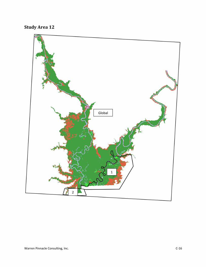
Warren Pinnacle Consulting, Inc. C-16
Study Area 12
Global
1
2
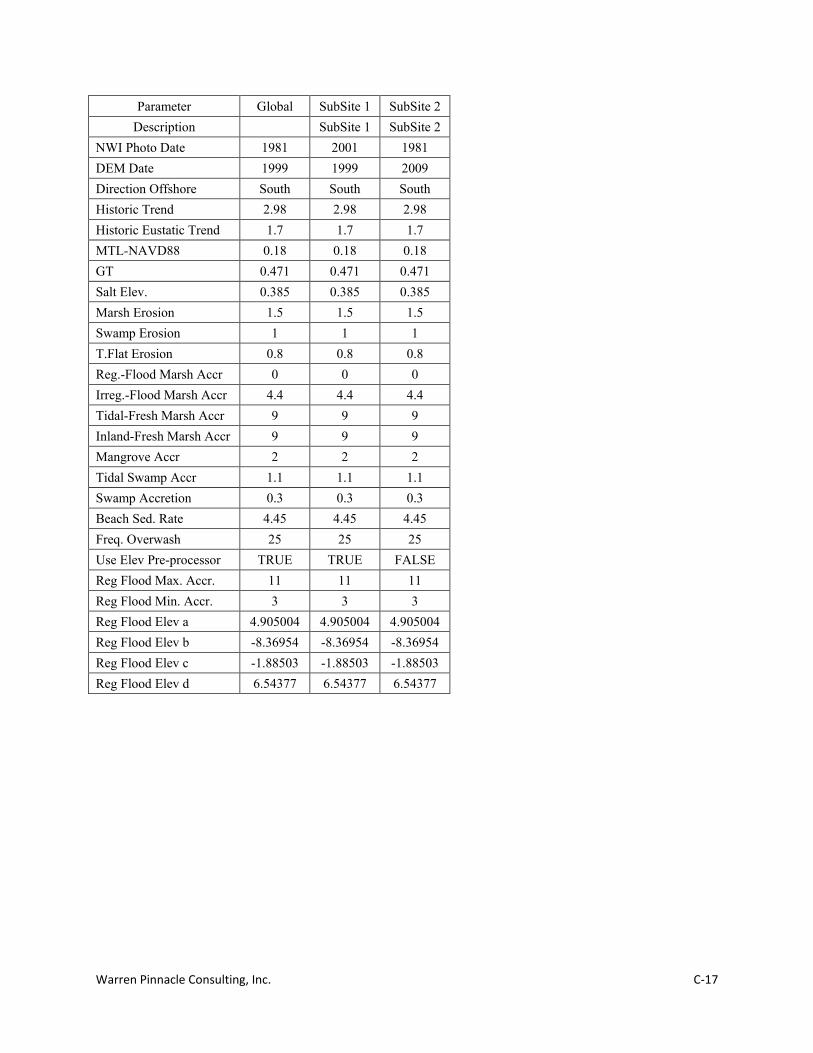
Warren Pinnacle Consulting, Inc. C-17
Parameter Global SubSite 1 SubSite 2 Description SubSite 1 SubSite 2
NWI Photo Date 1981 2001 1981 DEM Date 1999 1999 2009 Direction Offshore South South South Historic Trend 2.98 2.98 2.98 Historic Eustatic Trend 1.7 1.7 1.7 MTL-NAVD88 0.18 0.18 0.18 GT 0.471 0.471 0.471 Salt Elev. 0.385 0.385 0.385 Marsh Erosion 1.5 1.5 1.5 Swamp Erosion 1 1 1 T.Flat Erosion 0.8 0.8 0.8 Reg.-Flood Marsh Accr 0 0 0 Irreg.-Flood Marsh Accr 4.4 4.4 4.4 Tidal-Fresh Marsh Accr 9 9 9 Inland-Fresh Marsh Accr 9 9 9 Mangrove Accr 2 2 2 Tidal Swamp Accr 1.1 1.1 1.1 Swamp Accretion 0.3 0.3 0.3 Beach Sed. Rate 4.45 4.45 4.45 Freq. Overwash 25 25 25 Use Elev Pre-processor TRUE TRUE FALSE Reg Flood Max. Accr. 11 11 11 Reg Flood Min. Accr. 3 3 3 Reg Flood Elev a 4.905004 4.905004 4.905004 Reg Flood Elev b -8.36954 -8.36954 -8.36954 Reg Flood Elev c -1.88503 -1.88503 -1.88503 Reg Flood Elev d 6.54377 6.54377 6.54377

Warren Pinnacle Consulting, Inc. C-18
Study Area 14
Global
1
2
3 4
5
6
7 8
9
10
11
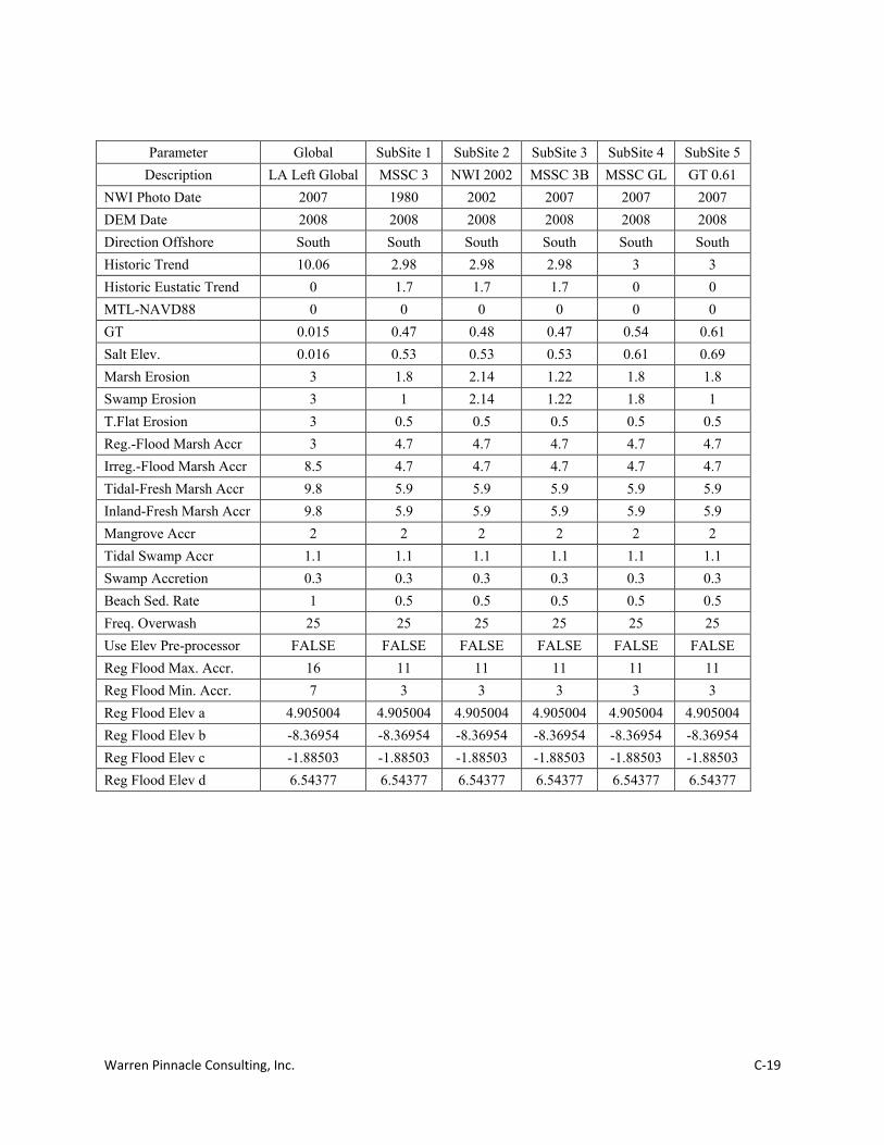
Warren Pinnacle Consulting, Inc. C-19
Parameter Global SubSite 1 SubSite 2 SubSite 3 SubSite 4 SubSite 5 Description LA Left Global MSSC 3 NWI 2002 MSSC 3B MSSC GL GT 0.61
NWI Photo Date 2007 1980 2002 2007 2007 2007 DEM Date 2008 2008 2008 2008 2008 2008 Direction Offshore South South South South South South Historic Trend 10.06 2.98 2.98 2.98 3 3 Historic Eustatic Trend 0 1.7 1.7 1.7 0 0 MTL-NAVD88 0 0 0 0 0 0 GT 0.015 0.47 0.48 0.47 0.54 0.61 Salt Elev. 0.016 0.53 0.53 0.53 0.61 0.69 Marsh Erosion 3 1.8 2.14 1.22 1.8 1.8 Swamp Erosion 3 1 2.14 1.22 1.8 1 T.Flat Erosion 3 0.5 0.5 0.5 0.5 0.5 Reg.-Flood Marsh Accr 3 4.7 4.7 4.7 4.7 4.7 Irreg.-Flood Marsh Accr 8.5 4.7 4.7 4.7 4.7 4.7 Tidal-Fresh Marsh Accr 9.8 5.9 5.9 5.9 5.9 5.9 Inland-Fresh Marsh Accr 9.8 5.9 5.9 5.9 5.9 5.9 Mangrove Accr 2 2 2 2 2 2 Tidal Swamp Accr 1.1 1.1 1.1 1.1 1.1 1.1 Swamp Accretion 0.3 0.3 0.3 0.3 0.3 0.3 Beach Sed. Rate 1 0.5 0.5 0.5 0.5 0.5 Freq. Overwash 25 25 25 25 25 25 Use Elev Pre-processor FALSE FALSE FALSE FALSE FALSE FALSE Reg Flood Max. Accr. 16 11 11 11 11 11 Reg Flood Min. Accr. 7 3 3 3 3 3 Reg Flood Elev a 4.905004 4.905004 4.905004 4.905004 4.905004 4.905004 Reg Flood Elev b -8.36954 -8.36954 -8.36954 -8.36954 -8.36954 -8.36954 Reg Flood Elev c -1.88503 -1.88503 -1.88503 -1.88503 -1.88503 -1.88503 Reg Flood Elev d 6.54377 6.54377 6.54377 6.54377 6.54377 6.54377

Warren Pinnacle Consulting, Inc. C-20
Parameter SubSite 6 SubSite 7 SubSite 8 SubSite 9 SubSite 10 SubSite 11 Description SubSite 6 SubSite 7 GL BS LA LEFT 11 Islands 6B
NWI Photo Date 2007 2007 2007 2007 2007 2007 DEM Date 2008 2008 2008 2008 2008 2008 Direction Offshore South South South South South South Historic Trend 5 9.44 9.44 9.44 2.98 3 Historic Eustatic Trend 0 1.7 1.7 1.7 1.7 0 MTL-NAVD88 0 0 0 0 0 0 GT 0.52 0.375 0.155 0.155 0.475 0.52 Salt Elev. 0.57 0.32 0.13175 0.13175 0.53 0.57 Marsh Erosion 2.2 0 1.8 1.8 3 2.4 Swamp Erosion 2.2 0 1 1 3 2.4 T.Flat Erosion 0.5 2 2 2 0.5 0.5 Reg.-Flood Marsh Accr 4.7 8.5 8.5 8.5 4.7 4.7 Irreg.-Flood Marsh Accr 4.7 8.5 8.5 8.5 4.7 4.7 Tidal-Fresh Marsh Accr 5.9 9.8 9.8 9.8 5.9 5.9 Inland-Fresh Marsh Accr 5.9 9.8 9.8 9.8 5.9 5.9 Mangrove Accr 2 2 2 2 2 2 Tidal Swamp Accr 1.1 8.2 8.2 8.2 1.1 1.1 Swamp Accretion 0.3 8.2 8.2 8.2 0.3 0.3 Beach Sed. Rate 0.5 1 1 1 0.5 0.5 Freq. Overwash 25 25 25 25 25 25 Use Elev Pre-processor FALSE FALSE FALSE FALSE FALSE FALSE Reg Flood Max. Accr. 11 16 16 16 11 11 Reg Flood Min. Accr. 3 6 6 6 3 3 Reg Flood Elev a 4.905004 4.905004 4.905004 4.905004 4.905004 4.905004 Reg Flood Elev b -8.36954 -8.36954 -8.36954 -8.36954 -8.36954 -8.36954 Reg Flood Elev c -1.88503 -1.88503 -1.88503 -1.88503 -1.88503 -1.88503 Reg Flood Elev d 6.54377 6.54377 6.54377 6.54377 6.54377 6.54377

Warren Pinnacle Consulting, Inc. C-21
Study Area 17
Global
1
2
3
4 5
6
7 8 9
11

Warren Pinnacle Consulting, Inc. C-22
Parameter Global SubSite 1 SubSite 2 SubSite 3 SubSite 4 SubSite 5
Description Muted 1 SubSite 2 SubSite 3 Vermillion
Bay Open
Ocean5 NWI Photo Date 2008 1988 1993 2008 2008 2008 DEM Date 2007 2007 2007 2007 2007 2007 Direction Offshore South South South South South South Historic Trend 10.06 10.06 10.06 10.06 10.06 10.06 Historic Eustatic Trend 0 0 0 0 0 0 MTL-NAVD88 0 0 0 0 0 0 GT 0.42 0.284 0.42 0.42 0.52 0.61 Salt Elev. 0.45 0.189 0.45 0.45 0.56 0.66 Marsh Erosion 3 3 3 3 2 9 Swamp Erosion 3 3 3 3 2 9 T.Flat Erosion 3 3 3 3 2 9 Reg.-Flood Marsh Accr 3 3 3 3 2 9 Irreg.-Flood Marsh Accr 8.5 8.5 8.5 8.5 8.5 8.5 Tidal-Fresh Marsh Accr 9.8 9.8 9.8 9.8 9.8 9.8 Inland-Fresh Marsh Accr 9.8 9.8 9.8 9.8 9.8 9.8 Mangrove Accr 2 2 2 2 2 2 Tidal Swamp Accr 1.1 1.1 1.1 1.1 1.1 1.1 Swamp Accretion 0.3 0.3 0.3 0.3 0.3 0.3 Beach Sed. Rate 1 1 1 1 1 1 Freq. Overwash 0 0 0 0 0 0 Use Elev Pre-processor FALSE FALSE FALSE FALSE FALSE FALSE Reg Flood Max. Accr. 16 16 16 16 16 16 Reg Flood Min. Accr. 7 7 7 7 7 7 Reg Flood Elev a 4.905004 4.905004 4.905004 4.905004 4.905004 4.905004 Reg Flood Elev b -8.36954 -8.36954 -8.36954 -8.36954 -8.36954 -8.36954 Reg Flood Elev c -1.88503 -1.88503 -1.88503 -1.88503 -1.88503 -1.88503 Reg Flood Elev d 6.54377 6.54377 6.54377 6.54377 6.54377 6.54377
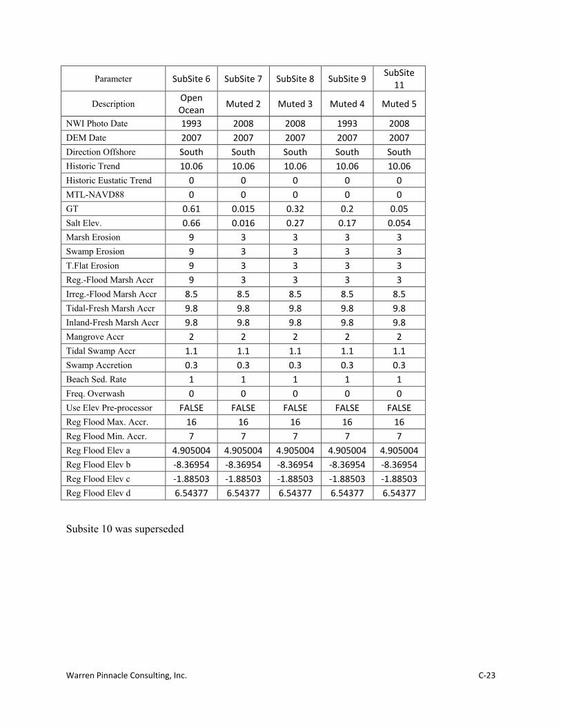
Warren Pinnacle Consulting, Inc. C-23
Parameter SubSite 6 SubSite 7 SubSite 8 SubSite 9 SubSite 11
Description Open Ocean Muted 2 Muted 3 Muted 4 Muted 5
NWI Photo Date 1993 2008 2008 1993 2008 DEM Date 2007 2007 2007 2007 2007 Direction Offshore South South South South South Historic Trend 10.06 10.06 10.06 10.06 10.06 Historic Eustatic Trend 0 0 0 0 0 MTL-NAVD88 0 0 0 0 0 GT 0.61 0.015 0.32 0.2 0.05 Salt Elev. 0.66 0.016 0.27 0.17 0.054 Marsh Erosion 9 3 3 3 3 Swamp Erosion 9 3 3 3 3 T.Flat Erosion 9 3 3 3 3 Reg.-Flood Marsh Accr 9 3 3 3 3 Irreg.-Flood Marsh Accr 8.5 8.5 8.5 8.5 8.5 Tidal-Fresh Marsh Accr 9.8 9.8 9.8 9.8 9.8 Inland-Fresh Marsh Accr 9.8 9.8 9.8 9.8 9.8 Mangrove Accr 2 2 2 2 2 Tidal Swamp Accr 1.1 1.1 1.1 1.1 1.1 Swamp Accretion 0.3 0.3 0.3 0.3 0.3 Beach Sed. Rate 1 1 1 1 1 Freq. Overwash 0 0 0 0 0 Use Elev Pre-processor FALSE FALSE FALSE FALSE FALSE Reg Flood Max. Accr. 16 16 16 16 16 Reg Flood Min. Accr. 7 7 7 7 7 Reg Flood Elev a 4.905004 4.905004 4.905004 4.905004 4.905004 Reg Flood Elev b -8.36954 -8.36954 -8.36954 -8.36954 -8.36954 Reg Flood Elev c -1.88503 -1.88503 -1.88503 -1.88503 -1.88503 Reg Flood Elev d 6.54377 6.54377 6.54377 6.54377 6.54377
Subsite 10 was superseded
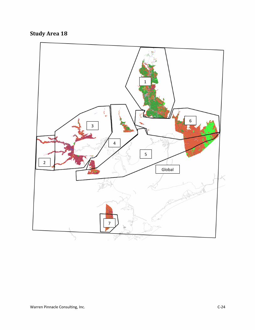
Warren Pinnacle Consulting, Inc. C-24
Study Area 18
Global
1
2
3
4
5
6
7

Warren Pinnacle Consulting, Inc. C-25
Parameter Global SubSite 1 SubSite 2 SubSite 3 SubSite 4
Description
DEM 2008
Trinity Delta
SubSite 2 Urban Tribs HSC
NWI Photo Date 2006 2006 1992 2006 2006 DEM Date 2009 2008 2009 2009 2009 Direction Offshore East South East East East Historic Trend 4.75 4.75 4.75 4.75 4.75 Historic Eustatic Trend 1.7 1.7 1.7 1.7 1.7 MTL-NAVD88 0.1224 0.1224 0.1224 0.1224 0.1224 GT 0.3444 0.3 0.4998 0.4998 0.4511 Salt Elev. 0.3508 0.38357 0.4324 0.4324 0.4068 Marsh Erosion 1 1 2.44 2.44 1 Swamp Erosion 1 1 2.44 2.44 1 T.Flat Erosion 1 1 2.44 2.44 1 Reg.-Flood Marsh Accr 7.75 7.75 7.75 7.75 7.75 Irreg.-Flood Marsh Accr 7.75 7.75 7.75 7.75 7.75 Tidal-Fresh Marsh Accr 2.9 2.9 2.9 2.9 2.9 Inland-Fresh Marsh Accr 2.9 2.9 2.9 2.9 2.9 Mangrove Accr 7 7 7 7 7 Tidal Swamp Accr 1.1 1.1 1.1 1.1 1.1 Swamp Accretion 0.3 0.3 0.3 0.3 0.3 Beach Sed. Rate 1 1 3 3 1 Freq. Overwash 30 30 30 30 30 Use Elev Pre-processor FALSE FALSE FALSE FALSE FALSE Reg Flood Max. Accr. 10 10 10 10 10 Reg Flood Min. Accr. 3.8 3.8 3.8 3.8 3.8 Reg Flood Elev a 4.977941 4.977941 4.977941 4.977941 4.977941 Reg Flood Elev b -13.3409 -13.3409 -13.3409 -13.3409 -13.3409 Reg Flood Elev c 3.930084 3.930084 3.930084 3.930084 3.930084 Reg Flood Elev d 9.692886 9.692886 9.692886 9.692886 9.692886
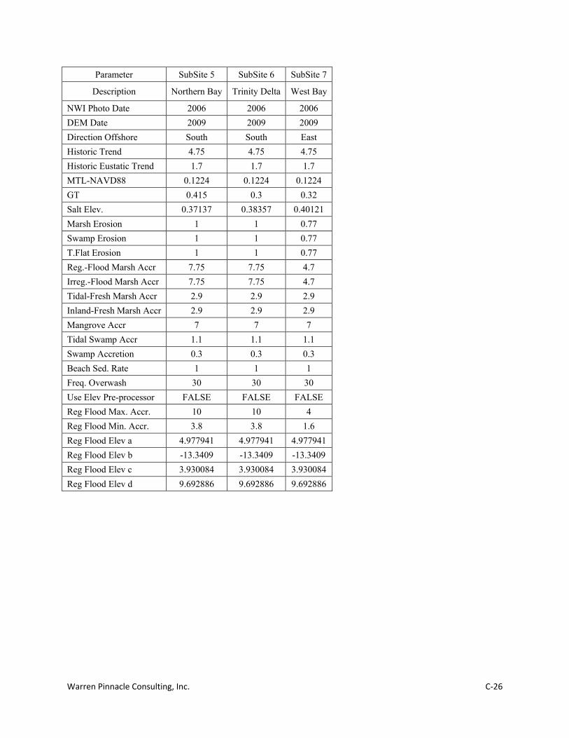
Warren Pinnacle Consulting, Inc. C-26
Parameter SubSite 5 SubSite 6 SubSite 7
Description Northern Bay Trinity Delta West Bay
NWI Photo Date 2006 2006 2006 DEM Date 2009 2009 2009 Direction Offshore South South East Historic Trend 4.75 4.75 4.75 Historic Eustatic Trend 1.7 1.7 1.7 MTL-NAVD88 0.1224 0.1224 0.1224 GT 0.415 0.3 0.32 Salt Elev. 0.37137 0.38357 0.40121 Marsh Erosion 1 1 0.77 Swamp Erosion 1 1 0.77 T.Flat Erosion 1 1 0.77 Reg.-Flood Marsh Accr 7.75 7.75 4.7 Irreg.-Flood Marsh Accr 7.75 7.75 4.7 Tidal-Fresh Marsh Accr 2.9 2.9 2.9 Inland-Fresh Marsh Accr 2.9 2.9 2.9 Mangrove Accr 7 7 7 Tidal Swamp Accr 1.1 1.1 1.1 Swamp Accretion 0.3 0.3 0.3 Beach Sed. Rate 1 1 1 Freq. Overwash 30 30 30 Use Elev Pre-processor FALSE FALSE FALSE Reg Flood Max. Accr. 10 10 4 Reg Flood Min. Accr. 3.8 3.8 1.6 Reg Flood Elev a 4.977941 4.977941 4.977941 Reg Flood Elev b -13.3409 -13.3409 -13.3409 Reg Flood Elev c 3.930084 3.930084 3.930084 Reg Flood Elev d 9.692886 9.692886 9.692886

Warren Pinnacle Consulting, Inc. C-27
Study Area 19
Global
1
2
3
4
5
6
7 8
9
10
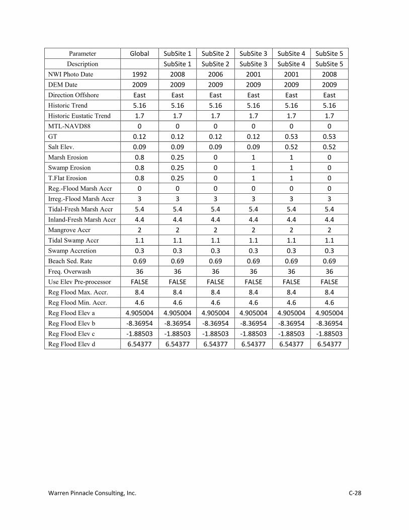
Warren Pinnacle Consulting, Inc. C-28
Parameter Global SubSite 1 SubSite 2 SubSite 3 SubSite 4 SubSite 5 Description
SubSite 1 SubSite 2 SubSite 3 SubSite 4 SubSite 5 NWI Photo Date 1992 2008 2006 2001 2001 2008 DEM Date 2009 2009 2009 2009 2009 2009 Direction Offshore East East East East East East Historic Trend 5.16 5.16 5.16 5.16 5.16 5.16 Historic Eustatic Trend 1.7 1.7 1.7 1.7 1.7 1.7 MTL-NAVD88 0 0 0 0 0 0 GT 0.12 0.12 0.12 0.12 0.53 0.53 Salt Elev. 0.09 0.09 0.09 0.09 0.52 0.52 Marsh Erosion 0.8 0.25 0 1 1 0 Swamp Erosion 0.8 0.25 0 1 1 0 T.Flat Erosion 0.8 0.25 0 1 1 0 Reg.-Flood Marsh Accr 0 0 0 0 0 0 Irreg.-Flood Marsh Accr 3 3 3 3 3 3 Tidal-Fresh Marsh Accr 5.4 5.4 5.4 5.4 5.4 5.4 Inland-Fresh Marsh Accr 4.4 4.4 4.4 4.4 4.4 4.4 Mangrove Accr 2 2 2 2 2 2 Tidal Swamp Accr 1.1 1.1 1.1 1.1 1.1 1.1 Swamp Accretion 0.3 0.3 0.3 0.3 0.3 0.3 Beach Sed. Rate 0.69 0.69 0.69 0.69 0.69 0.69 Freq. Overwash 36 36 36 36 36 36 Use Elev Pre-processor FALSE FALSE FALSE FALSE FALSE FALSE Reg Flood Max. Accr. 8.4 8.4 8.4 8.4 8.4 8.4 Reg Flood Min. Accr. 4.6 4.6 4.6 4.6 4.6 4.6 Reg Flood Elev a 4.905004 4.905004 4.905004 4.905004 4.905004 4.905004 Reg Flood Elev b -8.36954 -8.36954 -8.36954 -8.36954 -8.36954 -8.36954 Reg Flood Elev c -1.88503 -1.88503 -1.88503 -1.88503 -1.88503 -1.88503 Reg Flood Elev d 6.54377 6.54377 6.54377 6.54377 6.54377 6.54377
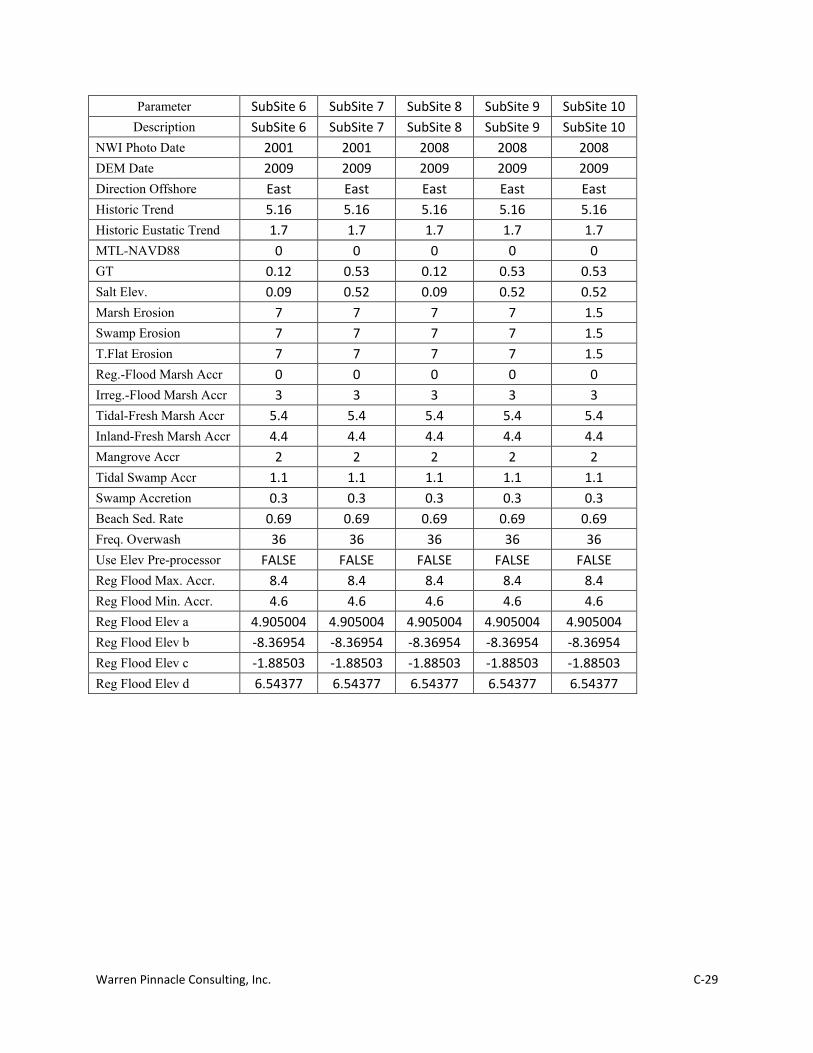
Warren Pinnacle Consulting, Inc. C-29
Parameter SubSite 6 SubSite 7 SubSite 8 SubSite 9 SubSite 10 Description SubSite 6 SubSite 7 SubSite 8 SubSite 9 SubSite 10
NWI Photo Date 2001 2001 2008 2008 2008 DEM Date 2009 2009 2009 2009 2009 Direction Offshore East East East East East Historic Trend 5.16 5.16 5.16 5.16 5.16 Historic Eustatic Trend 1.7 1.7 1.7 1.7 1.7 MTL-NAVD88 0 0 0 0 0 GT 0.12 0.53 0.12 0.53 0.53 Salt Elev. 0.09 0.52 0.09 0.52 0.52 Marsh Erosion 7 7 7 7 1.5 Swamp Erosion 7 7 7 7 1.5 T.Flat Erosion 7 7 7 7 1.5 Reg.-Flood Marsh Accr 0 0 0 0 0 Irreg.-Flood Marsh Accr 3 3 3 3 3 Tidal-Fresh Marsh Accr 5.4 5.4 5.4 5.4 5.4 Inland-Fresh Marsh Accr 4.4 4.4 4.4 4.4 4.4 Mangrove Accr 2 2 2 2 2 Tidal Swamp Accr 1.1 1.1 1.1 1.1 1.1 Swamp Accretion 0.3 0.3 0.3 0.3 0.3 Beach Sed. Rate 0.69 0.69 0.69 0.69 0.69 Freq. Overwash 36 36 36 36 36 Use Elev Pre-processor FALSE FALSE FALSE FALSE FALSE Reg Flood Max. Accr. 8.4 8.4 8.4 8.4 8.4 Reg Flood Min. Accr. 4.6 4.6 4.6 4.6 4.6 Reg Flood Elev a 4.905004 4.905004 4.905004 4.905004 4.905004 Reg Flood Elev b -8.36954 -8.36954 -8.36954 -8.36954 -8.36954 Reg Flood Elev c -1.88503 -1.88503 -1.88503 -1.88503 -1.88503 Reg Flood Elev d 6.54377 6.54377 6.54377 6.54377 6.54377
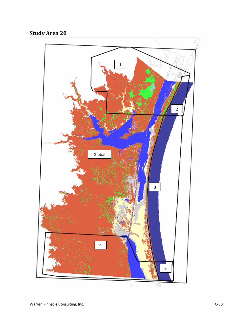
Warren Pinnacle Consulting, Inc. C-30
Study Area 20
Global
1
2
3
4
5

Warren Pinnacle Consulting, Inc. C-31
Parameter Global SubSite 1 SubSite 2 SubSite 3 SubSite 4 SubSite 5 Description
SubSite 1 SubSite 2 SubSite 3 SubSite 4 SubSite 5 NWI Photo Date 1993 2006 2006 1993 1993 1993 DEM Date 2010 2010 2010 2010 2010 2010 Direction Offshore East East East East East East Historic Trend 1.93 1.93 1.93 1.93 1.93 1.93 Historic Eustatic Trend 1.7 1.7 1.7 1.7 1.7 1.7 MTL-NAVD88 0 0 0 0 0 0 GT 0.06 0.06 0.56 0.56 0.06 0.56 Salt Elev. 0.045 0.045 0.55 0.55 0.045 0.55 Marsh Erosion 0 1.3 1.3 0 1.5 1.5 Swamp Erosion 0 1.3 1.3 0 1.5 1.5 T.Flat Erosion 0 1.3 1.3 0 1.5 1.5 Reg.-Flood Marsh Accr 0 0 0 0 0 0 Irreg.-Flood Marsh Accr 3 3 3 3 3 3 Tidal-Fresh Marsh Accr 5.38 5.38 5.38 5.38 5.38 5.38 Inland-Fresh Marsh Accr 4.4 4.4 4.4 4.4 4.4 4.4 Mangrove Accr 2 2 2 2 2 2 Tidal Swamp Accr 1.1 1.1 1.1 1.1 1.1 1.1 Swamp Accretion 0.3 0.3 0.3 0.3 0.3 0.3 Beach Sed. Rate 0.69 0.69 0.69 0.69 0.69 0.69 Freq. Overwash 50 50 50 50 50 50 Use Elev Pre-processor FALSE FALSE FALSE FALSE FALSE FALSE Reg Flood Max. Accr. 8.4 8.4 8.4 8.4 8.4 8.4 Reg Flood Min. Accr. 4.6 4.6 4.6 4.6 4.6 4.6 Reg Flood Elev a 4.905004 4.905004 4.905004 4.905004 4.905004 4.905004 Reg Flood Elev b -8.36954 -8.36954 -8.36954 -8.36954 -8.36954 -8.36954 Reg Flood Elev c -1.88503 -1.88503 -1.88503 -1.88503 -1.88503 -1.88503 Reg Flood Elev d 6.54377 6.54377 6.54377 6.54377 6.54377 6.54377