evaluation of pavement distresses appearance and ...€¦ · ahmed salah, talaat abdel-wahed civil...

http://www.iaeme.com/IJCIET/index.asp 197 [email protected]

International Journal of Civil Engineering and Technology (IJCIET) Volume 6, Issue 11, Nov 2015, pp. 197-208, Article ID: IJCIET_06_11_020

Available online at

http://www.iaeme.com/IJCIET/issues.asp?JType=IJCIET&VType=6&IType=11

ISSN Print: 0976-6308 and ISSN Online: 0976-6316

© IAEME Publication

___________________________________________________________________________

EVALUATION OF PAVEMENT DISTRESSES

APPEARANCE AND PROPAGATION FOR

URBAN ROADS IN UPPER EGYPT

Ahmed Salah, Talaat Abdel-Wahed

Civil Engineering Department, Faculty of Engineering, Sohag University, Egypt

Amr Whabla, Ayman Othman

Civil Engineering Department, Faculty of Engineering, Aswan University, Egypt

ABSTRACT

Monitoring and evaluating pavements condition have a multi benefits that

can be employed in maximizing network performance. It is used to evaluate

the applied maintenance strategies, generating prediction models that

describe performance trend in the future, and determining the trigger

threshold values for maintenance and rehabilitation (M, R) actions. Also, it

can be used for evaluating the quality of paving process and the design

criteria. A detailed distresses and traffic surveys were conducted for 60km of

urban roads of Sohag city in Upper Egypt. The geographical information

system GIS is used as a tool for storing the data. The overlay date of the

segments was obtained from the highway and bridges institute of Sohag. The

distresses recorded are raveling, bleeding, deformation (rutting and shoving),

longitudinal cracking, patching, and cut areas. The statistics analysis was

used to examine the relationship between each distress and the variables that

may affect in the appearance and propagation of it. Results showed that

raveling distress is function of traffic, age, and bleeding. However, bleeding

distress hasn’t any relationship with age or traffic. For deformation and

cracking, they are function only in bleeding. Results showed also, there is no

relationship between the appearances or propagation of bleeding,

deformation, cracking and different independent variables (age, cumulative

number of vehicles, cumulative weights of vehicles). In the other hand,a new

model for predicting raveling deduct value in housing cities in Upper Egypt.

Key words: Prediction model, Maintenance, Pavement distress, GSI,

Statistical analysis.

Ahmed Salah, Talaat Abdel-Wahed, Amr Whabla and Ayman Othman


Cite this Article: Ahmed Salah, Talaat Abdel-Wahed, Amr Whabla and Ayman

Othman. Evaluation of Pavement Distresses Appearance and Propagation for

Urban Roads in Upper Egypt, International Journal of Civil Engineering and

Technology, 6 (11), 2015, pp. 197-208.

http://www.iaeme.com/IJCIET/issues.asp?JType=IJCIET&VType=6&IType=11

1. LITERATURE REVIEW

Generating prediction models for pavement distresses explains the reasons of

distresses appearance and considered the heart of pavement maintenance management

system PMMS. There are three types of prediction models; empirical, mechanistic-

empirical, and probabilistic models. The last two types requires large number of

pavement segments which can be grouped in homogenous categories. So, they may be

not suitable for urban roads at small cities. Empirical models are developed by

regression analysis and more suitable for small networks. Many studies and agencies

use the regression analysis for developing prediction models which can be used in

evaluating various maintenance techniques and generating future maintenance plans.

(Hongmei Li)used the area under performance curve to evaluate the effectiveness

of the thin overlay and determine the application time. The rut depth was used as the

performance indicator to generate regression prediction models. The model showed

that rut depth was depending on age and traffic. Several regression models were used

to select the best curve estimation type (highest R2 and lowest P-value). It was found

that linear and cubic methods are the best fitting types.

(Kim and Kim) used data collected by Georgia department of transportation

GDOT to generate linear prediction models. The pavement condition evaluation

system PACES rating is a performance indicator defined by the agency and used to

monitor pavement condition. Prediction models were generated for interstate routes

and state highways separately. The interstate routs were grouped into 7 groups for

different 7 districts and the prediction models were developed for each district

separately. Three types of models were generated; one, two, and three variable

models. Variables used were age, AADT, and the product of age and AADT. The

regression analysis was conducted by Minitab program.It was found that higher R2

occurs if the relationship is between PACES index and age or the product of AADT

and age in one-variable model, for the two variable model,age and AADT or age and

the product of age and AADT.

(Lamptey, Labi, and Li)determined the optimal time for the application of

preventive maintenances along 30 years period. The maintenance actions studied were

thin overlay and micro-surfacing. The regression analysis was used to determine

models for the performance jump at the application year and the post-treatment

performance trend. The performance indicators used were surface roughness (IRI),

rutting (RUT), and pavement condition rating (PCR). For each performance indicator,

a PJ model was estimated as a function of pretreatment value for each treatment type.

The curve types used in the PJ trends were quadratic, logarithmic, and exponential.

The post treatment trend was an exponential model as a function of cumulative traffic

and cumulative freeze index. For each treatment type, a three different models for the

three performance indicators were developed. The R2 values for these models varies

from 0.41 to 0.71.

(Abo-Hashema and Sharaf) used a maintenance decision tool developed in Egypt

which select the appropriate maintenance and rehabilitation action M&R according to

the types and density of localized treatment actions required. For each localized

Evaluation of Pavement Distresses Appearance and Propagation for Urban Roads in

Upper Egypt


treatment action a maintenance unite MU value was selected. The summation of MU

values determine the suitable M&R activity. The total MU values for data collected

by LTTP (a long term pavement performance program conducted by the American

strategic highway research program) were calculated and tabulated against age. An

exponential model was developed for four environment categories. The developed

model predict the future MU values according to the current MU value and number of

years. The P-value was less than 0.05 but R2was also low for all models. The R

2

values were greatly improved after taking into account a traffic factor and the

structural number SN.

(Li et al.)determined the best time for the application of crack seal, chip seal,

slurry seal, and thin overlay. The performance indicators used were the IRI, rut depth,

and friction number. Seven variables were proposed to be significant in the prediction

values of the three indicators. These variables were the initial pavement condition,

environmental zone, traffic level, subgrade type, pavement age, maintenance age, and

time from the maintenance application. Linear regression was considered and the

ANOVA statistical analysis was applied. The variables that have P-value more than

0.1 were considered not significant. Three linear models were generated (one for each

performance indicator)for control sections (sections without any maintenance), slurry

seal sections, chip seal sections, thin overlay sections, and crack seal sections.

(Ding, Sun, and Chen) used an exponential model for the prediction of pavement

condition index PCI. The model predict the future PCI according to the current PCI

and age. The model used to determine the optimal maintenance strategy of a three

strategies. The three strategies were the do nothing, preventive maintenance, and

structural overlay (rehabilitation). It was found that the application of preventive

maintenance at PCI of 85 is the most cost effectiveness strategy.

(Yu et al.) developed a maintenance plans for a network that maximized

performance and minimized costs and the environmental effects. Four maintenance

actions were considered in the study; micro-surfacing, slurry seal, HMA overlay, and

mill & fill. A linear model was used for each of the four actions to describe the post-

treatment trends. The R2 of these models vary from 0.55 to 0.87.

(Ram) determined the effectiveness of some treatments applied in Michigan

department. The treatment used in the agency are single chip seal, double chip seal,

double micro-surfacing, crack seal, HMA mill and overlay, and HMA overlay.

Exponential regression models were used for pre-treatment performance and post-

treatment performance trends. The city was divided into two environmental zones. An

exponential prediction model was developed to predict the future distress index DI for

each treatment, environment zone, and pavement type. The R2 for models varied from

0.36 to 0.83.

In this study, the distresses of Sohag city was examined against traffic, age, and

traffic weights. Several regression techniques were used to discover the best fitting

type. A prediction models were derived for distresses that have clear relationship with

variables.

2. CASE STUDY AND DATA COLLECTION

According to the institute of highway and bridges in Sohag, the highway urban

network of Sohag aren’t recorded or monitored. So, the M&R actions are conducted

by the engineer’s experiences. A survey system was developed to record pavement

distresses and the variables that may affect in the appearance and propagation of these



distresses. A survey vehicle equipped with GPS, cameras, and laptop was used to

collect pavement images and coordinates of the network.

2.1. Network Referencing and Segmentation

The global positioning system (GPS) was used to reference and divide network into

small samples with 20 meter length. The coordinates every 10 meter lengthwere

picked up and saved. Every five consecutive samples are a management sample (i.e.

100 meter).

2.2. Imaging Process

The survey vehicle was equipped with two cameras. The first one was hanged at

about 2.5 meter above the pavement surface and record an image every 10 meter. The

second was hanged at one side of the vehicle and record an image for the road side

every 20 meter. This image described the start point of every data sample.

As survey vehicle traveling on the study road, the system picked up the

coordinates every 10 meter, takes an image for the pavement surface for this distance,

and takes an image for the road side every 20 meter.

2.3. Pavement Performance Index

The most appropriate index for representing performance for Egyptian urban roads is

the pavement condition index PCI which developed by ASTM. In this standard, 19

distress type and three severity level for each type are considered for the flexible

pavement. Each severity level for the certain distress type has a unique curve which

gives the deduct values DV every density percentage. The distresses quantifying

process is conducted by walking on the pavement shoulder and manually recording

the density percentage for each severity level for each distress type.(ASTM, 2003)

2.4. Sample Data

The data recorded for each sample were the road name, full width of road, traffic

lanes width, two pavement images, two images for the start and end point of the

sample, coordinates of the start and end points, and distresses survey data. The

coordinates and images were collected by the survey vehicle but the remaining data

were collected manually. Each management sample represents one point in the

distress analysis.

2.5. Traffic Survey

A traffic survey was conducted at points which have a significant change in traffic

volume on the surveyed network. Number of vehicles for each category was recorded

at the peak hour. The weights of vehicles were estimated from international index

called growth weight factor GWF and allowable trucks weight estimated by the

general authority of highways and bridges in Egypt. The cumulative number of

vehicles and the equivalent single axle load ESAL number along the pavement age

were calculated.

2.6. GIS Database

The data collected is a spatial data and non-spatial data. The two types of data were

related together by GIS system. A database model is developed on arcgis10.22

program on two essential layers. The first layer is the data samples layer which

records the street name, street ID, sample ID, the ID of the management segment that


http://www.iaeme.com/IJCIET/index.asp

accommodates the sample, lanes width, sample length, pavement images number, and

pavement distresses types and severities. A map was drawn by the coordinates of

samples. In this layer, the area of samples is c

distresses are derived from joined tables.

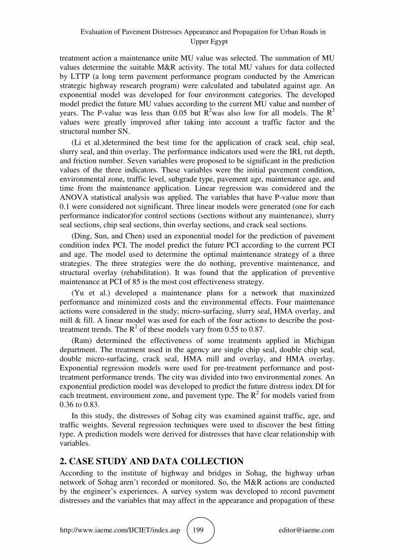
The second layer is the management segments layer which was drawn above the

data sample layer. This layer record management segment ID, segments age, full

width, lanes width, the accumulative vehicles per lane, and the accumulative ESAL

per lane. The two layers are spatially joined to calculate the average deduct values for

the management segments.

Figure 1

3. NETWORK CONDITION

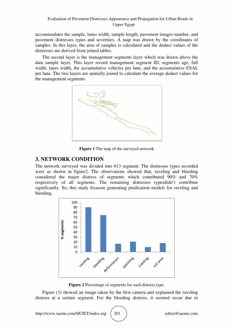
The network surveyed was divided into 613 segment. The distresses types recorded

were as shown in figure2. The observations showed that, raveling and bleeding

considered the major distress of segments which contributed 90% and 70%

respectively of all segments. The remaini

significantly. So, this study focus

bleeding.

Figure 2

Figure (3) showed an image taken by the first camera and explained

distress at a certain segment. For the bleeding distress, it seemed occur due to

0

10

20

30

40

50

60

70

80

90

100

% s

eg

me

nts


Upper Egypt

ET/index.asp 201 [email protected]



samples. In this layer, the area of samples is calculated and the deduct values of the

distresses are derived from joined tables.



, the accumulative vehicles per lane, and the accumulative ESAL


the management segments.

Figure 1 The map of the surveyed network

NETWORK CONDITION

eyed was divided into 613 segment. The distresses types recorded



respectively of all segments. The remaining distresses typesdidn’t

So, this study focuson generating predication models for raveling and

Percentage of segments for each distress type.

(3) showed an image taken by the first camera and explained



[email protected]



alculated and the deduct values of the



, the accumulative vehicles per lane, and the accumulative ESAL


eyed was divided into 613 segment. The distresses types recorded



typesdidn’t contribute

generating predication models for raveling and

(3) showed an image taken by the first camera and explained the raveling




excessive amount of bitumen during the paving process. It appears in new overlaid

segments with the full width and not restricted with wheel paths as shown in figure

(4).

Figure 3 Raveling distress at segment no.

(432)

Figure 4 Medium severity bleeding due to

excessive amount of bitumen

It is noticed also, most of segments that suffer from deformations (rutting and

shoving) have bleeding distress as shown in figure (5). Accordingly, these segments

are more susceptible to be deformed which the flow will increase and stability will

decrease.

Figure 5 Percentage of deformed segments at different bleeding levels

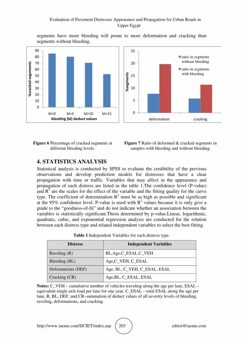
Furthermore, appearance of cracks almost accompanied with bleeding. The

observed cracks in the network are longitudinal cracks in the wheel paths. This kind

of distress occurs due to low stability of asphalt, and increasing bitumen level above

the designed percentage decreases the stability of asphalt. This illustrates the

appearance of cracking in these segments which have excessive bitumen as shown in

figure (6).A comparison between ratio of deformed and cracked segments in samples

with bleeding and without bleeding were made as shown in figure 7.It noticed that,

0

10

20

30

40

50

60

70

80

90

100

bl>0 bl>5 bl>10 bl>15

%d

efo

rme

d s

eg

me

nts

The deduct values of bleeding (bl)


Upper Egypt


segments have more bleeding will prone to more deformation and cracking than

segments without bleeding.

Figure 6 Percentage of cracked segments at

different bleeding levels.

Figure 7 Ratio of deformed & cracked segments in

samples with bleeding and without bleeding.

4. STATISTICS ANALYSIS

Statistical analysis is conducted by SPSS to evaluate the credibility of the previous

observations and develop prediction models for distresses that have a clear

propagation with time or traffic. Variables that may affect in the appearance and

propagation of each distress are listed in the table 1.The confidence level (P-value)

and R2 are the scales for the effect of the variable and the fitting quality for the curve

type. The coefficient of determination R2 must be as high as possible and significant

at the 95% confidence level. P-value is used with R2 values because it is only give a

guide to the “goodness-of-fit” and do not indicate whether an association between the

variables is statistically significant.Thisis determined by p-value.Linear, logarithmic,

quadratic, cubic, and exponential regression analysis are conducted for the relation

between each distress type and related independent variables to select the best fitting.

Table 1 Independent Variables for each distress type.

Distress Independent Variables

Raveling (R) BL,Age,C_ESAL,C_VEH

Bleeding (BL) Age,C_VEH, C_ESAL

Deformations (DEF) Age, BL, C_VEH, C_ESAL, ESAL

Cracking (CR) Age,BL, C_ESAL, ESAL

Notes: C_VEH – cumulative number of vehicles traveling along the age per lane, ESAL –

equivalent single axle load per lane for one year, C_ESAL – total ESAL along the age per

lane, R, BL, DEF, and CR–summation of deduct values of all severity levels of bleeding,

raveling, deformations, and cracking.

0

10

20

30

40

50

60

70

80

90

bl>0 bl>5 bl>10 bl>15

%cr

ack

ed

se

ge

me

nts

bleeding (bl) deduct values

0

5

10

15

20

25

deformation cracking

%se

gm

en

ts

ratio in segments

without bleeding

ratio in segments

with bleeding



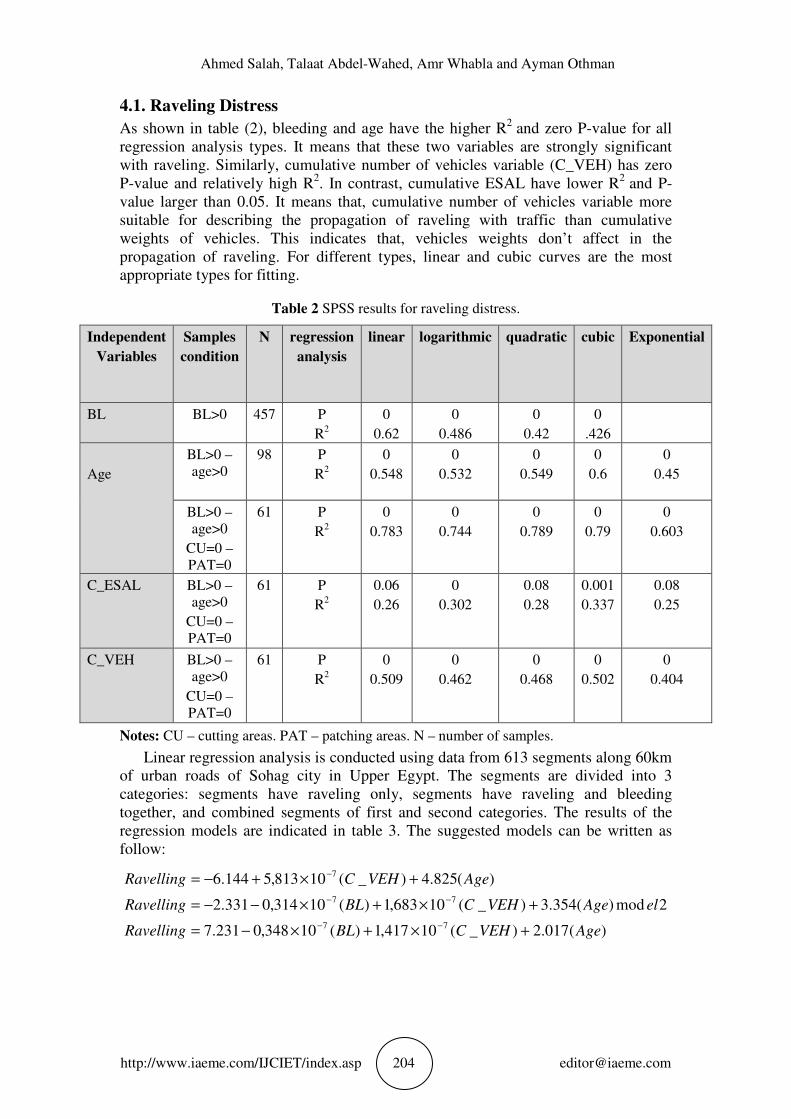
4.1. Raveling Distress

As shown in table (2), bleeding and age have the higher R2

and zero P-value for all

regression analysis types. It means that these two variables are strongly significant

with raveling. Similarly, cumulative number of vehicles variable (C_VEH) has zero

P-value and relatively high R2. In contrast, cumulative ESAL have lower R

2 and P-

value larger than 0.05. It means that, cumulative number of vehicles variable more

suitable for describing the propagation of raveling with traffic than cumulative

weights of vehicles. This indicates that, vehicles weights don’t affect in the

propagation of raveling. For different types, linear and cubic curves are the most

appropriate types for fitting.

Table 2 SPSS results for raveling distress.

Independent

Variables

Samples

condition

N regression

analysis

linear logarithmic quadratic cubic Exponential

BL BL>0 457 P

R2

0

0.62

0

0.486

0

0.42

0

.426

Age

BL>0 –

age>0

98 P

R2

0

0.548

0

0.532

0

0.549

0

0.6

0

0.45

BL>0 –

age>0

CU=0 –

PAT=0

61 P

R2

0

0.783

0

0.744

0

0.789

0

0.79

0

0.603

C_ESAL BL>0 –

age>0

CU=0 –

PAT=0

61 P

R2

0.06

0.26

0

0.302

0.08

0.28

0.001

0.337

0.08

0.25

C_VEH BL>0 –

age>0

CU=0 –

PAT=0

61 P

R2

0

0.509

0

0.462

0

0.468

0

0.502

0

0.404

Notes: CU – cutting areas. PAT – patching areas. N – number of samples.

Linear regression analysis is conducted using data from 613 segments along 60km

of urban roads of Sohag city in Upper Egypt. The segments are divided into 3

categories: segments have raveling only, segments have raveling and bleeding

together, and combined segments of first and second categories. The results of the

regression models are indicated in table 3. The suggested models can be written as

follow:

)(017.2)_(10417,1)(10348,0231.7

2mod)(354.3)_(10683,1)(10314,0331.2

)(825.4)_(10813,5144.6

77

77

7

AgeVEHCBLRavelling

elAgeVEHCBLRavelling

AgeVEHCRavelling

+×+×−=

+×+×−−=

+×+−=

−−

−−

−


Upper Egypt


Table 3 The linear regression prediction models of raveling distress.

Independent

Variables

Model1

constants

Model2

constants

Model3

constants

Constant

BL

C_VEH

Age

-6.144

0

5.813x10-7

4.825

2.331

-0.314

1.683x10-7

3.354

7.231

-0.348

1.417 x10-7

2.017

P-value 0 0 0

R2 0.82 0.724 0.674

Samples

condition

BL=0

CU=0

PAT=0

BL>0

CU=0

PAT=0

BL>0

CU=0

PAT=0

4.2. Bleeding Distress

Linear regression analysis is conducted to the relationship between bleeding distress

and independent variables. The results are indicated in table 4. There is no obvious

model can be suggested between bleeding distress and the independent variables. This

is due to the values of R2which are very low and P-value is higher than 0.05. This

indicate that, the appearance of bleeding isn’t affected by traffic or age and that

bleeding don’t propagate with time. This result agrees with field observations which

indicated previously.

Table 4 SPSS results for bleeding distress.

Independent

Variables

Samples

condition

N regression

analysis


Age

BL>0 –

R=0

Age>0

26 P-value

R2

0.45

0.02

0.452

0.024

0.56

0.024

0.6

0.024

0.58

0.013

C_VEH BL>0 –

R=0

Age>0

26 P-value

R2

0.32

0.031

0.28

0.034

0.38

0.039

0.47

0.048

BV

C_ESAL BL>0 –

R=0

Age>0

26 P-value

R2

0.27

0.03

0.22

0.023

0.30

0.051

0.038

0.177

BV

4.3. Deformations Distresses

Results recorded in table 5 indicate that there is no relationship between the

appearance or propagation of deformations and age. Zero values of P for vehicles

number, vehicles weights, and bleeding indicate that these variables are influential.

Low R2 values mean that no prediction models can be developed and the influence of

these variables on the propagation of the distress is random.



Table 5 SPSS results for deformation distresses.

Independent

Variables

Samples

condition

N regression

analysis


BL 613 P-value

R2

0

0.034

0

0.035

0

0.039

BL BL>0 –

DEF>0

90 P-value

R2

0.023

0.057

0.047

0.044

0.07

0.059

0.123

0.065

0.017

0.064

C_ESAL Age>0 332 P-value

R2

BV BV BV BV BV

C_ESAL Age>0 –

BL>0

234 P-value

R2

BV BV BV BV BV

C_ESAL Age>0 –

BL>0

DEF>0

90 P-value

R2

BV BV BV BV BV

age Age>0 227 P-value

R2

BV BV BV BV BV

C_VEH Age>0 227 P-value

R2

0.024

0.022

0.002

0.043

0.001

0.062

0.002

0.063

C_VEH Age>0 –

DEF>0

BL>0

90 P-value

R2

BV BV BV BV BV

ESAL 613 P-value

R2

0.017

0.009

0.005

0.013

0

0.027

0

0.035

ESAL DEF>0 102 P-value

R2

0.085

0.029

0.074

0.032

0.032

0.067

0.075

0.068

0.072

0.032

Although, the bleeding deduct value is varied from 0-10 to 10-20, the average

deformation D.V is still constant nearly as shown in table (6). However, for high

bleeding D.V (i.e. >20) the average deformation D.V increase clearly with low

average C_ESAL. It means that, with high bleeding, the pavement will prone to more

deformation with any amount of C_ESAL.

Table 6 Average deformations and traffic weights at each bleeding level.

Bleeding D.V Average deformation D.V Average C_ESAL

0 – 10 10.0304589 687027.8

10 – 20 11.5381714 610579.6

>20 23.127396 265120.1

4.4. Cracking Distress

The age of the most cracked segments isn’t available, so prediction model can’t be

developed for this distress. Results of SPSS indicated in table 6 show that bleeding


Upper Egypt


has a strong effect on the appearance and propagation of cracks. Traffic weights also

may be a significant factor. Cubic curve is the best fitting type for this distress as

shown in table (7).

Table 7 SPSS results for cracking distress.

Variabl

e

Samples

conditio

n

N regressio

n

analysis

linea

r

logarithmi

c

quadrati

c

cubi

c

Exponenti

al

BL 61

3

P-value

R2

0.006

0.012

0.005

0.017

0.00

6

0.02

BL CR>0 61 P-value

R2

0.715

0.002

0.05

0.1

0.00

3

0.22

0.75

0.02

BL CR>0 –

BL>0

52 P-value

R2

0.06

0.07

0.236

0.028

0.13

0.08

0.01

7

0.19

0.276

0.024

ESAL 61

3

P-value

R2

0

0.062

0.001

0.019

0

0.063

0

0.07

3

ESAL CR>0 61 P-value

R2

BV BV BV BV BV

5. CONCLUSIONS

This study shows that monitoring pavement distresses plays a vital role in evaluating

the paving process quality and developing prediction models for use in pavement

maintenance management systems. The study presents an evaluation for the distresses

categories, appearance, and propagation with time and traffic for small cities in Upper

Egypt. This evaluation is suitable for housing cities which haven’t significant

industrial activities where the percentage of trucks is very low. Most of segments have

raveling distress which considered aging distress not structural distress. The statistical

analysis shows that raveling increases with age and number of vehicles. A successful

linear prediction model is generated for raveling. The second popular distress is

bleeding which hasn’t any relation with age, number of vehicles, and traffic weights.

It appears in new segments and isn’t restricted with wheel paths. These observations

and SPSS results indicate that bleeding occurs due to the bad quality control during

the paving process. Rutting, shoving, and longitudinal cracks appear in small number

of segments which each distress appears in about 15% of segments. The observations

showed that 90% of segments which suffer from these distresseshave bleeding. The

statistics analysis of these structural distresses showed that they are sensitive for

bleeding and traffic weights and haven’t any relationship with age or any variable

which includes age. So any structural distresses in housing cities are due to bad

quality control during paving process.

6. RECOMMENDATIONS

The results of this study give some good recommendations for housing cities in Upper

Egypt as follow:



• A quality control system must be conducted during paving process to eliminate

excessive bleeding which may causes a structural distresses.

• A preventive maintenance activities such as fog seal, slurry seal, chip seal, and thin

overlay can be used as a treatment for raveling (the main distress in these cities).

• The cost effectiveness of these maintenance actions with age can be evaluated by

using prediction model developed in this study.

• A new segment without any bleeding will take about 8 years to be very rough and

needs a structural overlay. So applying preventive maintenances and conducting a

future maintenance plan will increases performance and decreases costs.

REFERENCE

[1] Abo-Hashema, Mostafa A, and Essam A Sharaf. “Development of Maintenance

Decision Model for Flexible Pavements.” International Journal of Pavement

Engineering 10.3 (2009): 173–187. Web.

[2] Ding, Tingting, Lijun Sun, and Zhang Chen. “Optimal Strategy of Pavement

Preventive Maintenance Considering Life-Cycle Cost Analysis.” Procedia -

Social and Behavioral Sciences 96.Cictp (2013): 1679–1685. Web.

[3] Hongmei Li, Fujian Ni. “Investigation into Application Time of Highway Asphalt

Pavement Preventive Maintenance Treatments.” Institute 2011 (2015): 3939–

3947. Print.

[4] Kim, By Sung-hee, and Nakseok Kim. “Development of Performance Prediction

Models in G Flexible Pavement G Using Regression Analysis Method.” 10.2

(2006): 91–96. Print.

[5] Lamptey, Geoffrey, Samuel Labi, and Zongzhi Li. “Decision Support for Optimal

Scheduling of Highway Pavement Preventive Maintenance within Resurfacing

Cycle.” Decision Support Systems 46.1 (2008): 376–387. Web.

[6] Li, Qiang et al. “Matter Element Analysis for Optimal Timing and Preventive

Maintenance of Pavements.” Transportation Research Record: Journal of the

Transportation Research Board 2150.1 (2010): 18–27. Web.

[7] Ram, Prashant V. “Performance and Benefits of Michigan DOT ’ S Capital

Preventive Maintenance Program.” Transportation Research Board 93rd Annual

Meeting. January 12-16, Washington, D.C. 994.2431 (2014): 1–17. Web.

[8] Salt, Modified, and Spray Fog. “Standard Practice for.” Evaluation (2007): 1–14.

Web.

[9] Yu, Bin et al. “Multi-Objective Optimization for Asphalt Pavement Maintenance

Plans at Project Level: Integrating Performance, Cost and Environment.”

Transportation Research Part D: Transport and Environment 41 (2015): 64–74.

Web.

[10] L.Vinoth Kumar and Dr.G.Umadevi.Advance Methodologies to Ensure Road

Safety, International Journal of Civil Engineering and Technology (IJCIET), 6

(6), 2015, pp. 158-164.

[11] Dr. K.V.Krishna Reddy. Influence of Subgrade Condition on Rutting in Flexible

Pavements- An Experimental Investigation, International Journal of Civil

Engineering and Technology (IJCIET), 4 (3), 2013, pp. 30-37.

evaluation of pavement distresses appearance and ...€¦ · ahmed salah, talaat abdel-wahed civil...

Documents